Master Thesis

Thermal Magnon Hall Effect in FM/AFMSkyrmionic Structures

Ilias Samathrakis

Supervised by:

Prof. Dr. Rembert Duine

December 2016

Institute for Theoretical Physics,

Leuvenlaan 4, 3584 CE Utrecht, The Netherlands

“I think nature’s imagination Is so much greater than man’s, she’s never going to

let us relax.”

– Richard Feynman.

Abstract

Inspired by Onose et al. [1], who observed the thermal magnon Hall effect in py-

rochlore ferromagnetic structures, the master Thesis in hand investigates the same

effect of magnons in stable, rectangular, ferromagnetic [2] and antiferromagnetic [3]

skyrmionic lattices. Our analysis is based on a Hamiltonian which consists of

the following four terms: an exchange interaction, an easy axis anisotropy, the

Dzyaloshinskii-Moriya interaction and an external magnetic field. Transformations

on the initial Hamiltonian in order to obtain the non-interacting magnonic spin-wave

Hamiltonian, and the standard method of diagonalisation, allow us to numerically

compute the effective magnetic field that the magnons feel, which is essential ingre-

dient to compute the transverse thermal conductivity.

The results found for both ferromagnetic and antiferromagnetic lattices show the

presence of the Hall effect of magnons at low temperatures. Although a direct

comparison between ferromagnets and antiferromagnets is impossible, since they

differ in the size as well as in the number of skyrmions, we do compare the two

configurations to conclude that the antiferromagnetic structure exhibits a stronger

Hall effect.

Page v

Table of Contents

Preface ix

List of Figures xi

List of Tables xiii

1 Introduction 1

1.1 The Hall Effect . . . . . . . . . . . . . . . . . . . . . . . . . . . . . . 1

1.2 Spintronics . . . . . . . . . . . . . . . . . . . . . . . . . . . . . . . . . 4

1.3 Magnons . . . . . . . . . . . . . . . . . . . . . . . . . . . . . . . . . . 5

1.4 Thermal Hall Effect . . . . . . . . . . . . . . . . . . . . . . . . . . . . 6

1.4.1 Berry Phase . . . . . . . . . . . . . . . . . . . . . . . . . . . . 7

1.4.2 Berry Curvature . . . . . . . . . . . . . . . . . . . . . . . . . 10

1.4.3 Skyrmions . . . . . . . . . . . . . . . . . . . . . . . . . . . . . 11

1.5 Literature Review . . . . . . . . . . . . . . . . . . . . . . . . . . . . . 14

2 Methodology 17

2.1 Theoretical Description: the Hamiltonian . . . . . . . . . . . . . . . . 17

2.1.1 Heisenberg Model . . . . . . . . . . . . . . . . . . . . . . . . . 18

2.1.2 Anisotropy Term . . . . . . . . . . . . . . . . . . . . . . . . . 19

2.1.3 Dzyaloshinskii-Moriya Interaction . . . . . . . . . . . . . . . . 20

2.1.4 External Magnetic Field . . . . . . . . . . . . . . . . . . . . . 21

2.2 Full Hamiltonian . . . . . . . . . . . . . . . . . . . . . . . . . . . . . 21

2.3 The Ground State . . . . . . . . . . . . . . . . . . . . . . . . . . . . . 21

2.4 Spin-wave Hamiltonian: Transformations . . . . . . . . . . . . . . . . 25

2.5 Diagonalisation of the Hamiltonian . . . . . . . . . . . . . . . . . . . 28

2.6 The Hall Conductivity . . . . . . . . . . . . . . . . . . . . . . . . . . 31

Page vii

2.6.1 Number of Magnons . . . . . . . . . . . . . . . . . . . . . . . 32

2.6.2 Effective Magnetic Field . . . . . . . . . . . . . . . . . . . . . 33

2.6.3 Adiabatic Approximation . . . . . . . . . . . . . . . . . . . . 38

2.6.4 Final Expression . . . . . . . . . . . . . . . . . . . . . . . . . 40

3 Results 41

3.1 Ferromagnets . . . . . . . . . . . . . . . . . . . . . . . . . . . . . . . 41

3.1.1 Dispersion . . . . . . . . . . . . . . . . . . . . . . . . . . . . . 41

3.1.2 Magnon Occupation . . . . . . . . . . . . . . . . . . . . . . . 42

3.1.3 Effective Magnetic Field . . . . . . . . . . . . . . . . . . . . . 42

3.1.4 Comparisons . . . . . . . . . . . . . . . . . . . . . . . . . . . 44

3.1.5 Hall Conductivity . . . . . . . . . . . . . . . . . . . . . . . . . 48

3.2 Antiferromagnets . . . . . . . . . . . . . . . . . . . . . . . . . . . . . 49

3.2.1 Dispersion . . . . . . . . . . . . . . . . . . . . . . . . . . . . . 49

3.2.2 Magnon Occupation . . . . . . . . . . . . . . . . . . . . . . . 49

3.2.3 Effective Magnetic Field . . . . . . . . . . . . . . . . . . . . . 50

3.2.4 Comparisons . . . . . . . . . . . . . . . . . . . . . . . . . . . 51

3.2.5 Hall Conductivity . . . . . . . . . . . . . . . . . . . . . . . . . 52

3.3 Comparisons and Conclusion . . . . . . . . . . . . . . . . . . . . . . . 53

4 Further Research 55

Appendices 57

A Ferromagnets and Antiferromagnets 59

B Magnon Dispersion Relation 61

C Chirality 67

Page viii

Preface

The Thesis in hand is the result of my 9-month effort for the partial fulfillment of

the master degree in Theoretical Physics of Utrecht University.

The general layout of this Thesis has been constructed in such a way to form an as

complete as possible guide to the topic of the magnon Hall effect to anyone who has

some basic background in quantum mechanics and physics. Hence, in the beginning

of Chapter 1, a short introduction to the Hall effect of charged particles is given.

Then, the field of spintronics is introduced to give to the reader a basic idea what

the topic is about, followed by the introduction to the notion of magnons, which

are important in this work. Next, the thermal Hall effect is discussed and apart

from this, the reader becomes familiar with some other important notions such as

the Berry curvature, the Berry Phase and skyrmions. The mosaic of Chapter 1 is

completed by a literature review, which consists of a discussion of relevant works of

other people. The purpose of the literature review is twofold. On the one hand it

reveals the uniqueness of this Thesis and on the other hand it connects it to previous

works.

Chapter 2, firstly deals with the Hamiltonian used by paying particular atten-

tion at each term of it separately. Once the Hamiltonian has been discussed, the

skyrmionic ground state of it, in both ferromagnets and antiferromagnets, is found.

Then, both the procedures of finding the spin-wave Hamiltonian and the way of

diagonalising it are briefly discussed. Since these methodologies are standard in

literature, the appropriate references are provided for the reader who wants to read

a rigorous mathematical explanation, which is outside of the scope of the Thesis.

Once the Hamiltonian is written in the notion of second quantisation operators

(spin-wave Hamiltonian), the procedure of extracting the transverse Hall conductivity

follows. More specifically, the number of magnons is computed followed by two ways

of computing the effective magnetic field.

Page ix

In Chapter 3 the results found using the theory and the methodology of Chap-

ter 2 are presented. In the beginning the dispersion relation of the Hamiltonian for

the two different cases is numerically computed, then the average magnon occupation

at each state is depicted in order to show the equivalence with Boson-Einstein statis-

tics. After that, the distribution of the magnetic field is given in order to finish with

the dependence of the thermal conductivity on temperature. The same procedure

is followed for the antiferromagnetic case and finally, some comparisons and the

conclusion of the Thesis is exported.

In Chapter 4 some open research questions and some possible extensions of the

present Thesis are discussed. Some of them might be useful for my future research

works and some others might inspire other people in order to continue working on

the specific topic.

Finally, in the appendix, the reader can find a very short introduction to the

ferromagnets and antiferromagnets, the derivation of magnon dispersion relation and

the notion of chirality. All of these introductory physics contribute to the better

understanding of the topic.

Having finished the tour over the chapter of my Thesis, I would like to thank

my supervisor Prof. Dr. Rembert Duine because with his passion for spintronics, he

subconsciously became my scientific role model and made me study hard in order

to learn a lot of very interesting topics. Rick Keesman for giving me his numerical

data and ultimately Jiansen Zheng and Patrick van Dieten for the very interesting

discussions that helped me to understand the topic deeper.

Ilias Samathrakis

Utrecht, December 13, 2016

Page x

List of Figures

1.1 The presence of the magnetic field influences the motion of the electrons

by forcing them to move in the y-direction. This effect is called the

Hall effect. . . . . . . . . . . . . . . . . . . . . . . . . . . . . . . . . . 2

1.2 Chain of spins (ground state). . . . . . . . . . . . . . . . . . . . . . . 5

1.3 Spin waves (taken from [4]). . . . . . . . . . . . . . . . . . . . . . . . 6

1.4 The presence of the temperature difference between the two sides trans-

ports heat current JQ as indicated in the picture. This phenomenon

is dubbed thermal Hall effect (taken from [5]). . . . . . . . . . . . . . 7

1.5 Time Zones (taken from [6]). . . . . . . . . . . . . . . . . . . . . . . . 8

1.6 Parallel Transport (taken from [7]). . . . . . . . . . . . . . . . . . . . 8

1.7 The phase difference between the two beams depends on the magnetic

flux inside the solenoid when the magnetic field is turned on. This

effect is known as the Aharonov-Bohm Effect (taken from [8]). . . . . 10

1.8 Domain walls and skyrmion number. . . . . . . . . . . . . . . . . . . 12

1.9 A ferromagnetic Skyrmion. . . . . . . . . . . . . . . . . . . . . . . . . 13

1.10 Magnetic phases of MnSi. The A-phase corresponds to the Skyrmion

phase (taken from [2]). . . . . . . . . . . . . . . . . . . . . . . . . . . 13

1.11 The crystal structure of Lu2V2O7 (taken from [1]). . . . . . . . . . . . 15

2.1 Initial lattice. . . . . . . . . . . . . . . . . . . . . . . . . . . . . . . . 22

2.2 The ferromagnetic Skyrmionic ground sate in three-dimensions. . . . 23

2.3 The ferromagnetic Skyrmionic ground sate in two-dimensions. . . . . 23

2.4 The antiferromagnetic Skyrmionic ground sate in three-dimensions. . 24

2.5 Two-dimensional visualisation of the antiferromagnetic Skyrmionic

ground state. . . . . . . . . . . . . . . . . . . . . . . . . . . . . . . . 25

2.6 Magnetic field of a lattice’s plaquette. . . . . . . . . . . . . . . . . . . 35

Page xi

2.7 Draft configuration. . . . . . . . . . . . . . . . . . . . . . . . . . . . . 37

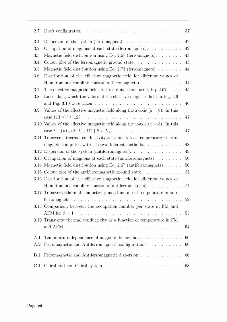
3.1 Dispersion of the system (ferromagnets). . . . . . . . . . . . . . . . . 42

3.2 Occupation of magnons at each state (ferromagnets). . . . . . . . . . 42

3.3 Magnetic field distribution using Eq. 2.67 (ferromagnets). . . . . . . . 43

3.4 Colour plot of the ferromagnetic ground state. . . . . . . . . . . . . . 43

3.5 Magnetic field distribution using Eq. 2.73 (ferromagnets). . . . . . . . 44

3.6 Distribution of the effective magnetic field for different values of

Hamiltonian’s coupling constants (ferromagnets). . . . . . . . . . . . 44

3.7 The effective magnetic field in three-dimensions using Eq. 2.67. . . . . 45

3.8 Lines along which the values of the effective magnetic field in Fig. 3.9

and Fig. 3.10 were taken. . . . . . . . . . . . . . . . . . . . . . . . . . 46

3.9 Values of the effective magnetic field along the x-axis (y = 8). In this

case 113 ≤ i ≤ 128 . . . . . . . . . . . . . . . . . . . . . . . . . . . . 47

3.10 Values of the effective magnetic field along the y-axis (x = 8). In this

case i ∈ kLx/2 | k ∈ N+ | k < Lx . . . . . . . . . . . . . . . . . . . 47

3.11 Transverse thermal conductivity as a function of temperature in ferro-

magnets computed with the two different methods. . . . . . . . . . . 48

3.12 Dispersion of the system (antiferromagnets). . . . . . . . . . . . . . . 49

3.13 Occupation of magnons at each state (antiferromagnets). . . . . . . . 50

3.14 Magnetic field distribution using Eq. 2.67 (antiferromagnets). . . . . . 50

3.15 Colour plot of the antiferromagnetic ground state. . . . . . . . . . . . 51

3.16 Distribution of the effective magnetic field for different values of

Hamiltonian’s coupling constants (antiferromagnets). . . . . . . . . . 51

3.17 Transverse thermal conductivity as a function of temperature in anti-

ferromagnets. . . . . . . . . . . . . . . . . . . . . . . . . . . . . . . . 52

3.18 Comparison between the occupation number per state in FM and

AFM for β = 1. . . . . . . . . . . . . . . . . . . . . . . . . . . . . . . 53

3.19 Transverse thermal conductivity as a function of temperature in FM

and AFM. . . . . . . . . . . . . . . . . . . . . . . . . . . . . . . . . . 54

A.1 Temperature dependence of magnetic behaviour. . . . . . . . . . . . . 60

A.2 Ferromagnetic and Antiferromagnetic configurations. . . . . . . . . . 60

B.1 Ferromagnetic and Antiferromagnetic dispersion. . . . . . . . . . . . . 66

C.1 Chiral and non Chiral system. . . . . . . . . . . . . . . . . . . . . . . 68

Page xii

List of Tables

2.1 Ground state coupling constants of Hamiltonian in Eq. 2.17 for ferro-

magnets. The coupling constants are in units of |J |. . . . . . . . . . . 22

2.2 Ground state coupling constants of Hamiltonian 2.17 in antiferromag-

nets. The coupling constants are in units of |J | . . . . . . . . . . . . 24

2.3 Explanation of symbols present in Eq. 2.74. . . . . . . . . . . . . . . 40

Page xiii

1

CHAPTER 1

Introduction

1.1 The Hall Effect

In this section, the Hall effect of charged particles is discussed, followed by the

derivation of a simple expression for the Hall coefficient. Even though the Hall effect

of charged particles is not the topic of the Thesis, it provides essential tools that we

use throughout the project.

The Hall effect was discovered in 1879 by Edwin Hall. It has to do with the produc-

tion of a voltage difference (known as the Hall voltage) across an electric conductor,

transverse to the electric field and a magnetic field perpendicular to the current. A

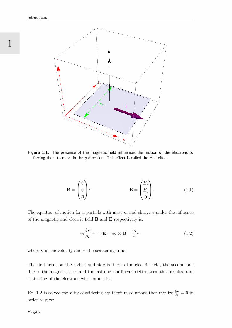
schematic representation of the Hall effect can be seen in Fig. 1.1.

In Fig. 1.1, the light blue area is the electric conductor, the green arrow points the

voltage and the black one the direction of the magnetic field. Finally, the purple

tube with the arrow shows the direction the electrons move.

As we can see in Fig. 1.1, electrons are restricted to move in (x, y) plane and the

magnetic field is in the z-direction. A constant current flows in the x-direction. Hall

effect states that this induces a voltage Vy in the y-direction. All these allow us to

write:

Page 1

Introduction

1

Figure 1.1: The presence of the magnetic field influences the motion of the electrons byforcing them to move in the y-direction. This effect is called the Hall effect.

B =

0

0

B

; E =

ExEy0

. (1.1)

The equation of motion for a particle with mass m and charge e under the influence

of the magnetic and electric field B and E respectively is:

m∂v

∂t= −eE− ev ×B− m

τv; (1.2)

where v is the velocity and τ the scattering time.

The first term on the right hand side is due to the electric field, the second one

due to the magnetic field and the last one is a linear friction term that results from

scattering of the electrons with impurities.

Eq. 1.2 is solved for v by considering equilibrium solutions that require ∂v∂t

= 0 in

order to give:

Page 2

1

Introduction

vx = −eτm

(Ex + vyB) ;

vy = −eτm

(Ey − vxB) ;

vz = 0. (1.3)

Using the definitions for the current density and the cyclotron frequency:

J = −nev;

ωB =eB

m,

with n the density of the charge carriers, we write Eq. 1.3 in matrix form as:

(1 ωBτ

−ωBτ 1

)(Jx

Jy

)=e2nτ

m

(Ex

Ey

). (1.4)

Ohm’s law suggests that

J = σE, (1.5)

with σ the conductivity. So, Eq. 1.4 can be written as:

σ =e2nτ

m

1

1 + ω2Bτ

2

(1 −ωBτωBτ 1

). (1.6)

The off-diagonal elements of this the matrix in Eq. 1.6 are responsible for the Hall

effect.

Multiplying both sides of Eq. 1.5 by σ−1 from the left and defining ρ = σ−1 (the

resistivity), we get:

E = ρJ, (1.7)

Page 3

Introduction

1

which is in the same form as Eq. 1.4, so(Ex

Ey

)=

(ρxx ρxy

ρyx ρyy

)(Jx

Jy

)⇔

(Ex

Ey

)=

(me2nτ

ωBme2n

−ωBme2n

me2nτ

)(Jx

Jy

). (1.8)

The Hall coefficient is defined as RH = EyBJx

evaluated in the limit Jy → 0, so using

Eq. 1.8 we write:

RH =ρxyB

=ωBm

Be2n=

1

ne. (1.9)

From this results we see that the Hall coefficient does not depend on the scattering

time. Therefore, the Hall effect is commonly used to experimentally determine the

density of charge carriers.

1.2 Spintronics

As far as we know electrons have two fundamental properties: charge and spin. The

first one has been measured and found equal to e and it has also been extensively

studied the past decades in order to give some spectacular silicon based applications

such as transistors. Most of these applications are based on the charge current, which

unfortunately has some significant drawbacks [1]:

The current is mediated by electrons, so some part of it is transferred to heat

because of the dissipation and therefore is lost → the energy-efficiency drops.

The electric charge has a specific unchanged value → not adjustable.

Charge interactions (Coulomb interactions) are quite strong → interference

problems.

A new generation of applications (for example data storage devices) may be con-

structed by using the other fundamental property of the electrons: spin. Spin is

widely known as the property which specifies whether a particle is a boson or a

fermion (integer or half-integer spin respectively) but it also has some other, non

trivial, properties, such as becoming the information carrier of a system. A relatively

new domain of physics which studies the “SPIN TRansport electrONICS”, or shorter

“spintronics”, sets its goal not only to make useful applications by using the spin

instead of the charge, but also to increase their efficiency. In this Thesis, wave-like

spin excitations, called magnons, are used as the information carrier. The notion of

magnon is presented in more details in the following section.

Page 4

1

Introduction

1.3 Magnons

The notion of magnon is necessary in order to proceed our tour in the very interesting

world of the magnon Hall effect. In the present section, two ways of approaching

magnons are discussed and the magnon dispersion relation is proven in the appendix.

The first approach has to do with the classical way of understanding them, whereas

the second one is purely quantum-mechanical.

The difficulty in understanding magnons arises from the fact that they are not “usual”

particles; instead, they are quasi-particles, collective excitations of the electron’s spin.

1. Semi-Classical approach:

One way to understand the notion of magnons is to consider them as elementary

excitations in ordered magnetic materials. Imagine an one-dimensional chain

of spins (ferromagnetic case for simplicity); as the one presented in Fig. 1.2.

The spins are orientated in the same upward direction and the system is at

its ground state. If now a single spin in the middle of the chain is flipped,

the system is not at its ground state anymore. Since this configuration is not

energetically favourable, other spins will also deviate from their initial position

in order to give rise to the lowest possible energy. In the end, the result is visible

in Fig. 1.3. The deviation is propagating in a wave-form manner, forming spin

waves (clear from the bottom part of Fig. 1.3). By using De Broglie’s relations

we can relate a particle to a wave and vise versa hence the quantised version of

the spin wave is the so called magnon quasi-particle [9].

Figure 1.2: Chain of spins (ground state).

Page 5

Introduction

1

Figure 1.3: Spin waves (taken from [4]).

2. Quantum approach:

Although the semi-classical approach explained before is simple, it is not

accurate enough since spins have no classical analogues. The full quantum

mechanical treatment requires the Holstein-Primakoff transformation which

map the spin operators to bosonic creation and annihilation operators (create

or annihilate a particle at a specific quantum state). In such a way, a spin

wave can be thought of as one quantum of a spin reversal spread coherently

over the system [10]. The interested reader can find the magnon dispersion

relation in the appendix of the Thesis.

1.4 Thermal Hall Effect

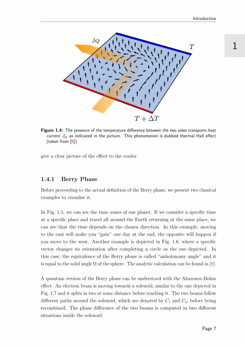
In this chapter we argue that the Hall effect of neutral quasiparticles such as magnons

exists and it is called Thermal Hall effect.

Magnons, as described in the previous section, are neutral quasiparticles. The

question that arises is whether they can exhibit the Hall effect. The answer to this

question is positive although they exhibit a different type of Hall effect dubbed

“Thermal Hall effect”. The basic difference between these two types is that in the

latter one, particles do not experience a magnetic field in Lorentz force, instead,

a temperature gradient ∇T transports a heat current JQ [11]. The whole idea is

illustrated in Fig. 1.4 (Fig. taken from [5]).

Magnons can travel in some magnetic configurations and pick up quantum-mechanical

phases that are dubbed “Berry Phases”, which give rise to “Berry Curvatures” that

act as an effective magnetic field [7] that they can feel. These configurations should

be skyrmionic in order to produce non vanishing Berry Curvatures.

The notions of “Berry Phase”, “Berry Curvature” and “Skyrmion” follow in order to

Page 6

1

Introduction

Figure 1.4: The presence of the temperature difference between the two sides transports heatcurrent JQ as indicated in the picture. This phenomenon is dubbed thermal Hall effect(taken from [5]).

give a clear picture of the effect to the reader.

1.4.1 Berry Phase

Before proceeding to the actual definition of the Berry phase, we present two classical

examples to visualise it.

In Fig. 1.5, we can see the time zones of our planet. If we consider a specific time

at a specific place and travel all around the Earth returning at the same place, we

can see that the time depends on the chosen direction. In this example, moving

to the east will make you “gain” one day at the end, the opposite will happen if

you move to the west. Another example is depicted in Fig. 1.6, where a specific

vector changes its orientation after completing a circle as the one depicted. In

this case, the equivalence of the Berry phase is called “anholonomy angle” and it

is equal to the solid angle Ω of the sphere. The analytic calculation can be found in [8].

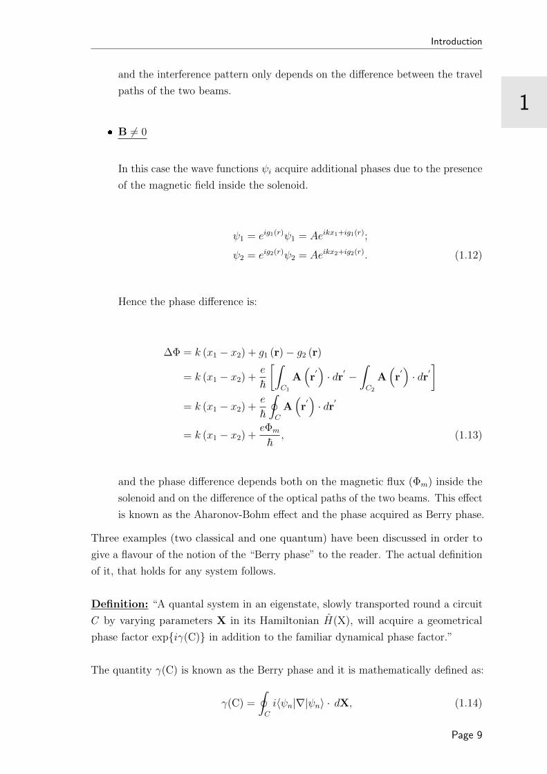
A quantum version of the Berry phase can be understood with the Aharonov-Bohm

effect. An electron beam is moving towards a solenoid, similar to the one depicted in

Fig. 1.7 and it splits in two at some distance before reaching it. The two beams follow

different paths around the solenoid, which are denoted by C1 and C2, before being

recombined. The phase difference of the two beams is computed in two different

situations inside the solenoid:

Page 7

Introduction

1

Figure 1.5: Time Zones (taken from [6]).

Figure 1.6: Parallel Transport (taken from [7]).

B = 0

In this case the wave functions ψi of the beams are given by plane waves of

the form:

ψ1 = Aeikx1 ;

ψ2 = Aeikx2 . (1.10)

Hence the phase difference is:

∆Φ = k (x1 − x2) , (1.11)

Page 8

1

Introduction

and the interference pattern only depends on the difference between the travel

paths of the two beams.

B 6= 0

In this case the wave functions ψi acquire additional phases due to the presence

of the magnetic field inside the solenoid.

ψ1 = eig1(r)ψ1 = Aeikx1+ig1(r);

ψ2 = eig2(r)ψ2 = Aeikx2+ig2(r). (1.12)

Hence the phase difference is:

∆Φ = k (x1 − x2) + g1 (r)− g2 (r)

= k (x1 − x2) +e

~

[∫C1

A(r′)· dr′ −

∫C2

A(r′)· dr′

]= k (x1 − x2) +

e

~

∮C

A(r′)· dr′

= k (x1 − x2) +eΦm

~, (1.13)

and the phase difference depends both on the magnetic flux (Φm) inside the

solenoid and on the difference of the optical paths of the two beams. This effect

is known as the Aharonov-Bohm effect and the phase acquired as Berry phase.

Three examples (two classical and one quantum) have been discussed in order to

give a flavour of the notion of the “Berry phase” to the reader. The actual definition

of it, that holds for any system follows.

Definition: “A quantal system in an eigenstate, slowly transported round a circuit

C by varying parameters X in its Hamiltonian H(X), will acquire a geometrical

phase factor expiγ(C) in addition to the familiar dynamical phase factor.”

The quantity γ(C) is known as the Berry phase and it is mathematically defined as:

γ(C) =

∮C

i〈ψn|∇|ψn〉 · dX, (1.14)

Page 9

Introduction

1

Figure 1.7: The phase difference between the two beams depends on the magnetic fluxinside the solenoid when the magnetic field is turned on. This effect is known as theAharonov-Bohm Effect (taken from [8]).

where ψn is the nth-eigenstate of the Hamiltonian H(X).

The interested reader can find more information about the Aharonov-Bohm effect

in [12].

1.4.2 Berry Curvature

Berry phase was defined in section 1.4.1 and more specifically from Eq. 1.14. A closer

look to the mathematical definition of the Berry phase, will reveal its strangeness.

The Berry phase itself (left hand side of the definition) is a meaningful quantity,

which can be observed experimentally. However, the integrand (which is called the

Berry connection) seems arbitrary and without any physical meaning [12]. In order

to overcome this problem, we can think of our Berry connection as of an abstract

vector potential An (X) known as the Berry vector potential. The definition of the

Berry phase now becomes:

γ(C) =

∮C

An (X) · dX. (1.15)

Stokes’ theorem allows us to write:

γ(C) = −∫∫

B (X) · n dσ, (1.16)

Page 10

1

Introduction

where the B-field is defined as:

Bn (X) = ∇×An (X) , (1.17)

and it is an observable quantity in the electromagnetic theory.

In the general case now, let us symbolise Berry connection with χn, such that:

χn = i〈ψn|∇|ψn〉. (1.18)

The analogue of the magnetic field now is given by an antisymmetric tensor field

called curvature (Berry curvature in this case).

Ωµν (X) = ∂Xµχnν − ∂Xνχnµ, (1.19)

which gives rise to:

Ωn (X) = ∇× χ (X) . (1.20)

The quantity Ω is called Berry curvature.

1.4.3 Skyrmions

Since the configurations needed to produce non vanishing Berry curvature are

skyrmionic, the notion of skyrmion is introduced.

The notion of “skyrmions” can be easier understood if we first introduce the “topo-

logical charge” or “Skyrmion number” as:

n =1

4π

∫M ·

(∂M

∂x× ∂M

∂y

)dx dy, (1.21)

where M is the unit spin direction vector.

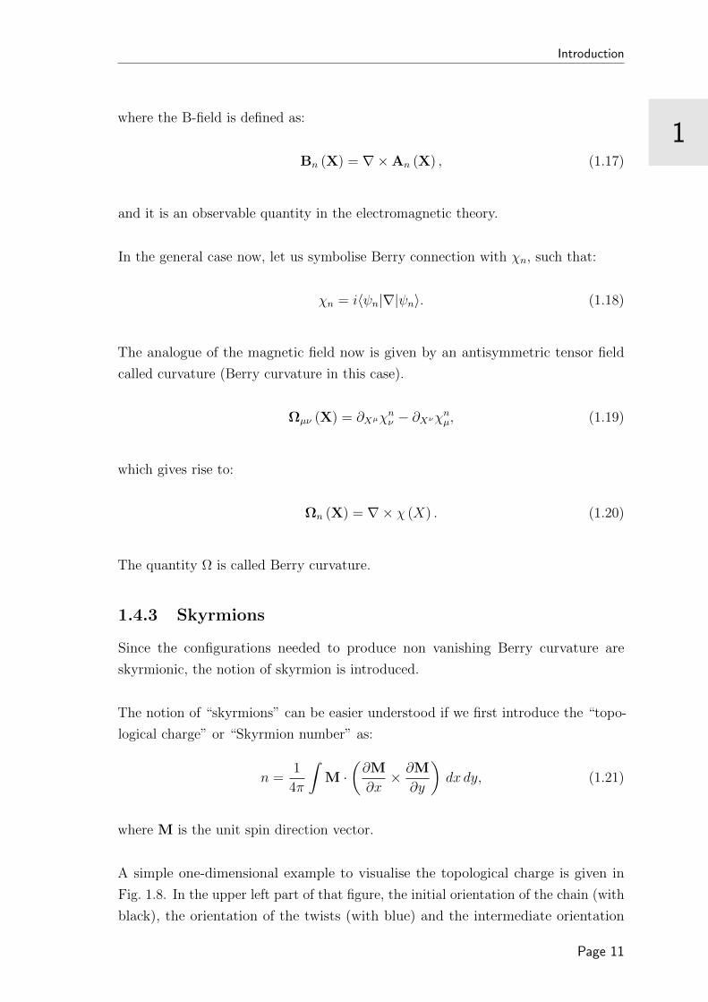
A simple one-dimensional example to visualise the topological charge is given in

Fig. 1.8. In the upper left part of that figure, the initial orientation of the chain (with

black), the orientation of the twists (with blue) and the intermediate orientation

Page 11

Introduction

1

(with red) are presented. As it is clear, the twist does not rotate over 360 degrees.

Unlike the upper part, the bottom chain is rotated over 360 degrees. The progressive

result of both chains are depicted in the right part of Fig. 1.8. In the first case we

observe n1 = 0, whereas in the second one n2 = 1.

0 4 8 12 16 200

π

2

π

spin

2πS

0 4 8 12 16 200

π

2 π

spin

2πS

Figure 1.8: Domain walls and skyrmion number.

The value of the topological charge “n” characterises if a configuration is a skyrmion

or not. More specifically, a configuration for which “n” takes a non vanishing and

integer value is called skyrmion [13].

An example of a two-dimensional skyrmion in a spin lattice can be seen in Fig. 1.9.

It has to be mentioned that these “constructions” are energetically favourable in

some materials (as discussed in more detail further on) which means that they are

stable as well. Muhlbauer et al. [2] found the magnetic phases of MnSi and their

results show evidence for the stability of the Skyrmionic phase in a magnetic material

(see Fig. 1.10).

Page 12

1

Introduction

Figure 1.9: A ferromagnetic Skyrmion.

Figure 1.10: Magnetic phases of MnSi. The A-phase corresponds to the Skyrmion phase(taken from [2]).

Mathematically speaking, skyrmions are examples of a specific class of solitons that

cannot decay due to topological protection. Solitons are a certain type of solutions of

several partial differential equations such as the Sine-Gordon and the Landau-Lifshitz

that are given respectively by:

Page 13

Introduction

1 ∂2u (x, t)

∂t2− ∂2u (x, t)

∂x2+ sinu (x, t) = 0;

(1.22)

dM

dt= −γM×Heff − λM× (M×Heff ) .

One can think of solitons as wave packets that move through a dispersive and

nonlinear medium, while changing neither their shape nor their velocity [14].

1.5 Literature Review

In this section, the work that has already been done is summarised and the uniqueness

of the work presented in this Thesis is stressed.

In order to be able to investigate the thermal Hall effect of magnons in skyrmionic

structures, we first have to prove that:

Magnon spin current indeed exists, which means that magnons can be used as

information carriers.

Skyrmionic structures that are going to be used as the initial configuration

both exist and they are stable.

Hence, the scientific progress in these two topics (information carrier and in lattices)

is relevant to the present Thesis and therefore it is discussed.

Information Carrier:

As explained in section 1.2 charge has some significant drawbacks in being the carrier

of information. The same holds for spins mainly because it is a property of electrons.

In recent year though, another candidate has dramatically increased its awareness

of becoming the information carrier; and this is the magnon, the current of which

has been shown to be possible by means of the spin Seebeck effect as explained by

Uchida et al. [15] and in the spin Hall effect as explained by Kajiwara et al. [16].

Magnons are probably better suited candidates since they are less subject to heating

and furthermore because its quasiparticle bosonic nature allows us to ignore losses due

to scattering phenomena at least at low temperatures, as Meier et al. have shown [17].

Page 14

1

Introduction

Lattice:

Muhlbauer et al. [2] have shown that ferromagnetic Skyrmionic structures are stable

in MnSi (phase A in their diagram, which is also mentioned in subsection 2.4).

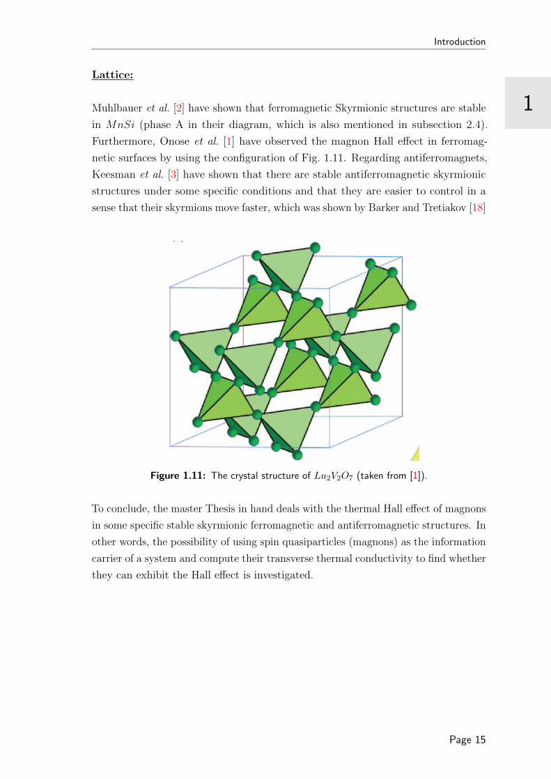
Furthermore, Onose et al. [1] have observed the magnon Hall effect in ferromag-

netic surfaces by using the configuration of Fig. 1.11. Regarding antiferromagnets,

Keesman et al. [3] have shown that there are stable antiferromagnetic skyrmionic

structures under some specific conditions and that they are easier to control in a

sense that their skyrmions move faster, which was shown by Barker and Tretiakov [18]

Figure 1.11: The crystal structure of Lu2V2O7 (taken from [1]).

To conclude, the master Thesis in hand deals with the thermal Hall effect of magnons

in some specific stable skyrmionic ferromagnetic and antiferromagnetic structures. In

other words, the possibility of using spin quasiparticles (magnons) as the information

carrier of a system and compute their transverse thermal conductivity to find whether

they can exhibit the Hall effect is investigated.

Page 15

2CHAPTER 2

Methodology

In this section the methodology followed to obtain the final results is discussed. The

Hamiltonian is first introduced and each term of it is analysed. Then, the ground

state which will be used as the initial configuration is given. Next, the methodology

of finding the spin-wave Hamiltonian, which involves some transformations, follows.

Thereafter, the standard method of diagonalising Hamiltonians of these type is briefly

discussed (the quick reader can skip subsection 2.5). Finally, a detailed explanation

of the procedure of the Hall conductivity was computed is presented.

2.1 Theoretical Description: the Hamiltonian

The system under consideration is a magnetic system, hence the energy is determined

by the interactions of the spins. In addition to these interactions, an external

magnetic field contributes as well. Therefore, the Hamiltonian takes the form:

H = Hint +Hext, (2.1)

where the subscripts “int” and “ext” correspond to the internal and the external

contribution respectively.

Internal Part:

The internal part of the Hamiltonian is due to the spin interaction among

Page 17

Methodology

2

particles. In general it reads:

Hint =∑i,j

STi VijSj, (2.2)

with Vij the interaction matrix given by:

Vij =

Vij

11 V ij12 V ij

13

V ij21 V ij

22 V ij23

V ij31 V ij

32 V ij33

. (2.3)

External Part:

The external part is only due to the presence of the external magnetic field

and its contribution to the Hamiltonian is:

Hext = B∑i

(Si)z . (2.4)

In order to simplify the interaction matrix Vij of the internal part of the Hamiltonian,

we can write it as follows [19, 20]:

Vij = Jij + V+ij + V−ij, (2.5)

where Jij is the exchange term, V+ij is the anisotropic exchange (symmetric, traceless)

and V−ij is the Dzyaloshinskii-Moriya interaction (antisymmetric). Each of these

terms contributes differently to the Hamiltonian and further analysis is provided in

the following subsections.

2.1.1 Heisenberg Model

The first term on the right hand side of Eq. 2.5 is defined as (taken from [19]):

Jij =Tr (Vij)

3, (2.6)

which corresponds to the isotropic part of the interaction matrix and it is called

“exchange integral”.

Page 18

2

Methodology

The Heisenberg model is the simplest model that can mathematically describe spin

interactions quantum mechanically and it is present in all magnetic systems. The

general form of the Hamiltonian is:

Hgen = −∑i 6=j

JijSi · Sj. (2.7)

In our case there are two additional restrictions that simplify this term.

The interactions between particles have no preference in the direction, which

practically means that Jij can be simply written as J (it does not depend on

the indices).

There are only interactions between nearest neighbouring sites. This is mathe-

matically expressed by the sum∑〈i,j〉.

Under these conditions the Hamiltonian is:

HHM = −J∑〈i,j〉

Si · Sj. (2.8)

The interested reader can find more information and the complete derivation of the

exchange term [21].

2.1.2 Anisotropy Term

The second term on the right hand side of Eq. 2.5 is defined as (taken from [19]):

V+ij =

Vij + VTij

2− Jij, (2.9)

which corresponds to a symmetric traceless part and it is called “anisotropic ex-

change”.

Unlike the exchange integral of the previous subsection, the anisotropic exchange

has a minor contribution and it is computationally demanding, therefore only an

important part of it will be taken into account and the rest will be neglected.

The important part is the on-site term V+ii hence, the Hamiltonian reads:

HA =∑i

STi KiSi, (2.10)

with Ki the lattice anisotropy tensor.

Page 19

Methodology

2

As in the previous subsection, there are two additional simplifications that make the

term easier.

The lattice anisotropy tensor Ki is the same at any position of the lattice.

The anisotropy only exists in the z-direction.

Under these simplifications the Hamiltonian can be written in an easier way as:

HA = −K∑i

(S2i

)z. (2.11)

2.1.3 Dzyaloshinskii-Moriya Interaction

The third term on the right hand side of Eq. 2.5 is defined as (taken from [19]):

V−ij =Vij −VT

ij

2, (2.12)

which corresponds to the antisymmetric part of the interaction matrix.

Since V−ij is by definition antisymmetric, we can express it as a Three-dimensional

vector, using the formula:

(V−ij)mn

=3∑l=1

Dijl εlmn, (2.13)

with εlmn to be the Levi-Civita symbol and Dij the Dzyaloshinskii vector. So:

HDMI =∑〈i,j〉

STi V−ijSj =∑〈i,j〉

Di,j · (Si × Sj) . (2.14)

This term is based on chiral symmetries [22] since the Dzyaloshinskii vector van-

ishes when the system faces inversion symmetry [21] and it was initially derived

by Dzyaloshinskii in 1960. It also theoretically explains the phase A in Fig.1.10.

After Moriya’s contribution the term has been named as the Dzyaloshinskii-Moriya

spin-orbit interaction which is one of the ways to create Skyrmions [23]. Further

analysis will reveal that this term tries to force Si and Sj to be at a right angle in a

plane perpendicular to the vector D.

An important simplification that makes this term much easier is to assume that the

amplitude of the interaction is the same regardless the direction. This does not mean

Page 20

2

Methodology

though that the vector Dij points always to the same direction. The Dzyaloshinskii

vector Dij that we consider in this Thesis is given by:

Dij =

(0, D, 0) if j is the “left” neighbour of i

(0,−D, 0) if j is the “right” neighbour of i

(D, 0, 0) if j is the “above” neighbour of i

(−D, 0, 0) if j is the “below” neighbour of i

; (2.15)

where D is the Dzyaloshinskii-Moriya coupling.

2.1.4 External Magnetic Field

As explained before, the external part of the Hamiltonian is only due the the presence

of the magnetic field. This magnetic field stabilises the configuration and it is also

responsible for the Zeeman effect. In this Thesis, it has been taken parallel to the

z-direction (B = Bz).

2.2 Full Hamiltonian

As it has become clear, the full Hamiltonian will be given by the sum of all the

previously mentioned parts.

H = HHM +HA +HDMI +Hext. (2.16)

Therefore:

H = −J∑〈i,j〉

Si · Sj −K∑i

(S2i

)z+∑〈i,j〉

Di,j · (Si × Sj)−B∑i

(Si)z . (2.17)

2.3 The Ground State

Onose et al. [1] used the pyrochlore ferromagnetic structure of Lu2V2O7 in order to

observe the thermal magnon Hall effect. In this Thesis, the shape of the ground state

used is simpler. A two-dimensional lattice with dimensions Lx = 16 and Ly = 16

with periodic one-side boundary conditions for the ferromagnets and a 32× 32 with

full periodic boundary conditions for the antiferromagnets have been used. Fig. 2.1

illustrates the shape of the initial configuration for both cases (the total number of

spins is different). Each lattice site at this figure corresponds to the initial point of

the three-dimensional spin vector.

Page 21

Methodology

2

(Ly − 1)Lx + 1 (Ly − 1)Lx + 2 (Ly − 1)Lx + 3 · · · LyLx...

......

......

2Lx + 1 2Lx + 2 2Lx + 3 · · · 3LxLx + 1 Lx + 2 Lx + 3 · · · 2Lx

1 2 3 · · · Lx

Figure 2.1: Initial lattice.

Given specific values to the couplings in the Hamiltonian of Eq. 2.17, the ground

states were found using Monte Carlo Simulations performed by R. Keesman. In the

following part of this section, two ways of visualising the ground states will be given.

In the first one each spin vector is coloured in respect to its direction whereas in the

second one each spin vector at each lattice point is associated to a colour in such a

way the the deviations from the plane are determined according to the given colour

explanation adjacent to the figure.

Ferromagnets:

For the values of couplings shown in Table 2.1, the ground state has one skyrmion.

Coupling Numerical

Constant Value[|J |]

J 1.0

D 0.598833

K 0.0

B 0.1793

Table 2.1: Ground state coupling constants of Hamiltonian in Eq. 2.17 for ferromagnets. Thecoupling constants are in units of |J |.

Keesman et al. [24] showed that this skyrmionic ground state is stable. The two

different ways of visualising this configurations, as explained before, are shown in

Fig. 2.2 and Fig. 2.3. respectively.

Page 22

2

Methodology

Figure 2.2: The ferromagnetic Skyrmionic ground sate in three-dimensions.

0 2 4 6 8 10 12 140

5

10

15

xa

y a

Ground State

0.5

1

1.5

Figure 2.3: The ferromagnetic Skyrmionic ground sate in two-dimensions.

Antiferromagnets:

Regarding the antiferromagnetic case, the couplings that give rise to an eight-skyrmion

ground state are given in Table 2.2.

Page 23

Methodology

2

Coupling Numerical

Constant Value[|J |]

J −1.0

D 0.760216

K 0.0

B 3.2

Table 2.2: Ground state coupling constants of Hamiltonian 2.17 in antiferromagnets. Thecoupling constants are in units of |J |

The stability is proven by Keesman et al. [3]. Similarly to the ferromagnetic case,

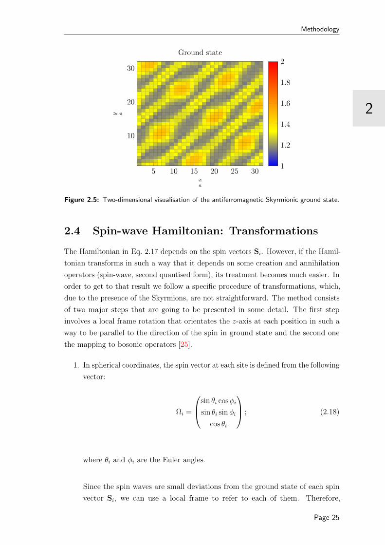
the two ways of visualisation are shown in Fig. 2.4 and Fig. 2.5 respectively.

Figure 2.4: The antiferromagnetic Skyrmionic ground sate in three-dimensions.

Page 24

2

Methodology

5 10 15 20 25 30

10

20

30

xa

y a

Ground state

1

1.2

1.4

1.6

1.8

2

Figure 2.5: Two-dimensional visualisation of the antiferromagnetic Skyrmionic ground state.

2.4 Spin-wave Hamiltonian: Transformations

The Hamiltonian in Eq. 2.17 depends on the spin vectors Si. However, if the Hamil-

tonian transforms in such a way that it depends on some creation and annihilation

operators (spin-wave, second quantised form), its treatment becomes much easier. In

order to get to that result we follow a specific procedure of transformations, which,

due to the presence of the Skyrmions, are not straightforward. The method consists

of two major steps that are going to be presented in some detail. The first step

involves a local frame rotation that orientates the z-axis at each position in such a

way to be parallel to the direction of the spin in ground state and the second one

the mapping to bosonic operators [25].

1. In spherical coordinates, the spin vector at each site is defined from the following

vector:

Ωi =

sin θi cosφi

sin θi sinφi

cos θi

; (2.18)

where θi and φi are the Euler angles.

Since the spin waves are small deviations from the ground state of each spin

vector Si, we can use a local frame to refer to each of them. Therefore,

Page 25

Methodology

2

multiplying each spin vector by a rotation matrix U is required [26].

Si = UiSi. (2.19)

This rotation matrix U in terms of the Euler angles is given by:

Ui =

cos θi cosφi cos θi sinφi − sin θi

− sinφi cosφi 0

cosφi sin θi sin θi sinφi cos θi

. (2.20)

For future reference, we compute the inverse matrix, which reads:

U−1i =

cos θi cosφi − sinφi cosφi sin θi

cos θi sinφi cosφi sin θi sinφi

− sin θi 0 cos θi

. (2.21)

Plugging Eq. 2.19 in the Hamiltonian 2.17, we get:

H = −J∑〈i,j〉

Si · UiU−1j Sj −K

∑i

(U−1i Si

)2

z

−B∑i

(U−1i Si

)z

+∑〈i,j〉

Di,j · [(U−1i Si

)×(U−1j Sj

)]; (2.22)

which is more compactly written as:

H = −1

2

∑i 6=j

JFαβij SiαSjβ +

1

2

∑i 6=j

Dijγ G

γαβij SiαSjβ

+K∑i

Gzαi G

zβi SiαSiβ −B

∑i

Gzαi Siα. (2.23)

In the Hamiltonian 2.23, Gγαβij are given by:

Gxαβij = Gyα

i Gzβj −Gzα

i Gyβj ;

Gyαβij = Gxα

i Gzβj −Gzα

i Gxβj ;

Gzαβij = Gxα

i Gyβj −G

yαi G

xβj ,

(2.24)

Page 26

2

Methodology

and Gαβi from:

U−1i =

Gxxi Gxy

i Gxzi

Gyxi Gyy

i Gyzi

Gzxi Gzy

i Gzzi

. (2.25)

Furthermore, Fαβij from:

UiU−1j =

Fxxij F xy

ij F xzij

F yxij F yy

ij F yzij

F zxij F zy

ij F zzij

. (2.26)

2. So far, Hamiltonian 2.23 is written in terms of the local frame used, although it

is not yet a function of creation and annihilation operators a† and a. Using first

the relations between the components of the spin vector and the spin creation

and annihilation operators, which are the following:

Sx = S++S−2

;

Sy = S+−S−2i

,(2.27)

allows us to map the spin operators S± to bosonic annihilation and creation

operators a and a† respectively by using the Holstein-Primakoff transforma-

tions [27]. These transformations were Taylor-expanded up to the first order

to give Eq. 2.28. The expansion holds if 1S 1 which means that S 1.

S+ = ~√

2S√

1− a†a2S

a ' ~√

2S a;

S− = ~√

2S a†√

1− a†a2S' ~√

2S a†;

Sz = ~(S − a†a

).

(2.28)

So, by combining Eq. 2.27 and Eq. 2.28, we can write:

Sx =√

2S~2

(a+ a†

);

Sy =√

2S~2i

(a− a†

);

Sz = ~(S − a†a

).

(2.29)

Hence, the final form of the Hamiltonian in Eq. 2.30 is obtained after some

lengthy calculations (contribution from P. van Dieten), where Eq. 2.29 is

substituted in Eq. 2.23 to get to the final form of the Hamiltonian (Eq. 2.30),

which reads:

Page 27

Methodology

2

H =∑〈ij〉

[tija†iaj + t∗ijaia

†j + τija

†ia†j + τ ∗ijaiaj]

+∑i

[mia†iai +m∗i aia

†i + µia

†ia†i + µ∗i aiai] + E0, (2.30)

where tij, τij, mi and µi are given by:

tij =

√SiSj

4[Dij

γ

(Gγxxij +Gγyy

ij − iGγxyij + iGγyx

ij

)− J

(F xxij + F yy

ij − iFxyij + iF yx

ij

)];

τij =

√SiSj

4[Dij

γ

(Gγxxij −G

γyyij + iGγxy

ij + iGγyxij

)− J

(F xxij − F

yyij + iF xy

ij + iF yxij

)];

mi =1

2KSi (G

zxi G

zxi +Gzy

i Gzyi ) +

1

2λi;

µi =1

2KSi (G

zxi G

zxi −G

zyi G

zyi + iGzx

i Gzyi − iG

zyi G

zxi ) ;

λi =∑j∈ni

JSjFzzij −

∑j∈ni

Dijγ SjG

γzzij − 2KSiG

zzi G

zzi +BGzz

i . (2.31)

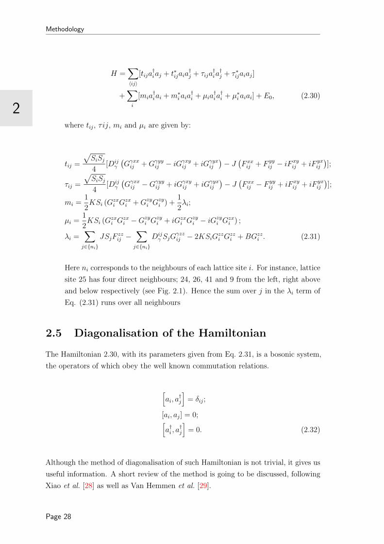
Here ni corresponds to the neighbours of each lattice site i. For instance, lattice

site 25 has four direct neighbours; 24, 26, 41 and 9 from the left, right above

and below respectively (see Fig. 2.1). Hence the sum over j in the λi term of

Eq. (2.31) runs over all neighbours

2.5 Diagonalisation of the Hamiltonian

The Hamiltonian 2.30, with its parameters given from Eq. 2.31, is a bosonic system,

the operators of which obey the well known commutation relations.

[ai, a

†j

]= δij;

[ai, aj] = 0;[a†i , a

†j

]= 0. (2.32)

Although the method of diagonalisation of such Hamiltonian is not trivial, it gives us

useful information. A short review of the method is going to be discussed, following

Xiao et al. [28] as well as Van Hemmen et al. [29].

Page 28

2

Methodology

The general form of a quadratic bosonic Hamiltonian reads:

H =∑i,j

αijc†icj +

1

2γijc

†ic†j +

1

2γ∗ijcicj. (2.33)

Eq. 2.33 can be more compactly written as:

H =1

2ψ†Mψ − 1

2tr (α) , (2.34)

where ψ, ψ† and M are given by:

ψ =

(c

c†

); ψ† =

(c† c)

; M =

(α γ

γ† α

), (2.35)

where c is the transpose of c and it is given by:

c =

c1

c2

...

cn

; c† =(c†1 c

†2 . . . c†n

). (2.36)

Let us for simplicity define

ci · cj = [ci, cj] , (2.37)

that allows us to rewrite the bosonic commutation relations (2.32) as:

ψ · ψ† = I−, (2.38)

with I− to be defined as:

I− =

(I 0

0 −I

). (2.39)

The Bogoliubov-Valatin transformation is then performed by

c = Ad+Bd†, (2.40)

Page 29

Methodology

2

where d is given as:

d =

d1

d2

...

dn

; d† =(d†1 d

†2 . . . d†n

). (2.41)

This gives rise to:

φ · φ† = I−, (2.42)

with:

φ =

(d

d†

); φ† =

(d† d

). (2.43)

Combining Eq. 2.36, 2.40 and 2.41, we can find

ψ = Tφ; T =

(A B

B∗ A∗

). (2.44)

Then, the Hamiltonian can be written as:

H =1

2φ†T †MTφ− 1

2tr (α) , (2.45)

and Eq. 2.38 is now written as:

TI−T† = I−. (2.46)

For the Hamiltonian 2.45 to be diagonal, it is necessary for T †MT to be diagonal.

T †MT =

ω1 0 0 · · · 0

0 ω2 0 · · · 0...

......

. . ....

0 0 0 · · · ω2n

. (2.47)

Page 30

2

Methodology

So under these conditions we have:

H =1

2

n∑i=1

(ωi − ωn+i) d†idi +

1

2

n∑i=1

ωn+i −1

2tr (α) . (2.48)

This is the so-called diagonal form of the Hamiltonian 2.33, with d†i and di bosonic

operators. The interested reader can read more about the diagonalisation proce-

dure [29], [28] and [30].

2.6 The Hall Conductivity

In this chapter we find the relation that describes the thermal Hall effect of magnons

in terms of quantities that we can numerically compute.

In section 1.1 the Hall effect of charged particles was discussed and the transverse

conductivity was found to be given from Eq. 1.6. However, this equation cannot be

used to describe the thermal Hall effect of magnons because:

1. It strictly depends on the charge of the particles and as we have seen magnons

are neutral quasiparticles.

2. It requires the presence of a Lorentz type magnetic force which is absent in

the thermal Hall effect of magnons.

Matsumoto et al. [31] have proven a formula which relates the transverse thermal

conductivity for neutral particles (or quasiparticles) with quantities that can be

computed. This formula reads:

κxy = −k2BT

~V∑n,k

c2 (ρn) Ωn,z (k) . (2.49)

To make things worse, this equation cannot be used since our ground states are

skyrmionic and the magnon Hamiltonian is not diagonalised by means of Fourier

transform because the presence of the skyrmion lattice breaks translation symmetry .

As discussed in section 2.2 the Hamiltonian of the system consists of four different

terms (exchange interactions, DM interaction, anisotropy term and external magnetic

field). The presence of the DMI is fruitful because it makes the system lack inversion

symmetry and it leads to the creation of chiral magnons with nontrivial topological

Page 31

Methodology

2

properties [11]. Furthermore, the presence of the DMI generates configurations with

non vanishing Berry curvature, which acts as an effective magnetic field [7] (Eq. 1.20),

that magnons can feel, giving rise to the thermal Hall effect.

Therefore, the thermal conductivity will firstly depend on Berry curvature (i.e. the

effective magnetic field) and secondly on the number of magnons excited. It has to

be mentioned that a strict mathematical formula for the Hall conductivity requires

techniques that are beyond the level of the Thesis hence we are only interested in

the trend of the the thermal conductivity.

After stating these rules, we are ready to give the simplest mathematical relation

which connects the transverse thermal conductivity with the number of magnons

and the effective magnetic field and it reads:

κxy ∝ nmBeff , (2.50)

where nm is the number of magnons and Beff the effective magnetic field.

Below, we present the method followed to obtain these two quantities. The number

of magnons is discussed in 2.6.1, subsequently, two ways to compute the effective

magnetic field are intrduced. The first one in section 2.6.2 while the latter one in

section 2.6.3.

2.6.1 Number of Magnons

In section 2.5 we showed that magnons are bosons, since their operators obey the

standard commutation relations. This is extremely important because it allows us

to compute the average number of some bosons at each state using Bose-Einstein

statistics. The relation which gives us the average number is given by:

ρi (εi) =1

eβεi − 1. (2.51)

where ρi stands for the average, i runs over all possible energy states of the system,

β = 1kBT

the inverse temperature with kB the Boltzmann constant and εi the energy

of each level. It can be easily understood that the total number of particles N of a

system which consists of r energy levels will be the sum of the average number of

Page 32

2

Methodology

particles at all levels:

N =r∑i=0

ρi (εi) =r∑i=0

1

eβεi − 1. (2.52)

Regarding magnon number we have to compute, the procedure is similar but more

complicated. First of all, in section 2.5 the eigenvalues ωi of the Hamiltonian were

computed. Since the method is based on doubling the Hamiltonian of the system,

we are only interested in half of the eigenvalues, the ones that correspond to positive

values, due to the positive definiteness of the matrix. This means that the eigenvalues

ωi are sorted in ascending order, which are labeled as ωi. Furthermore, the different

cases (ferromagnets and antiferromagnets) differ in the number of modes as well

because the first mode of the antiferromagnetic lattice corresponds to translation

motion of lattice and therefore it is neglected. In order to be able to write a general

formula for both cases, we have to introduce a new symbol, inspired from Kronecker’s

delta. This symbol is defined as:

δc,AFM =

1, if c = AFM

0, if c 6= AFM.(2.53)

Similarly, we can define:

δc,FM =

1, if c = FM

0, if c 6= FM.(2.54)

As it is obvious c ∈ FM,AFM.

Therefore, using Eq. 2.52 we can write:

nm,c =

2Lx,cLy,c∑a=Lx,cLy,c+1+δc,AFM

1

eβ~ωα,c − 1, (2.55)

with nm,c to be the total number of magnons of our system. The index α runs from

Lx,cLy,c + 1 + δc,AFM up to 2Lx,cLy,c because we are interested in the second half of

the eigenvalues.

2.6.2 Effective Magnetic Field

Next, the procedure to find the effective magnetic field Beff is discussed.

Page 33

Methodology

2

The Hamiltonian of the system (Eq. 2.30) can be written as:

H =m∑

i,j=1

(a†i aj

)(Hij

)(aja†i

). (2.56)

The method of diagonilisation (analysed in section 2.5) implies that the Hamiltonian

matrix Hij is written as:

(Hij) =

A B

B∗ A∗

;

with A and B sub-matrices responsible for the a†iaj (and aia†j) and aiaj (and a†ia

†j)

part of the Hamiltonian respectively.

From now on, we only focus on the top left part of the Hamiltonian matrix Hij [32],

which is for simplicity denoted by Aij and it is the matrix containing the hopping

amplitudes. Henceforth, the Hamiltonian is approximated as:

Hij ≈ Aij. (2.57)

Considering this approximation and the so called Peierls substitution:

tij → tijeie

∫ ji Adr, (2.58)

where the integral in the exponent is the phase a particle acquires while moving from

the point “i” of the lattice to the adjacent point “j” [33], we write the Hamiltonian

matrix as [34, 35]:

Hij = Aijeiφij . (2.59)

In order to eliminate the tunneling amplitude Aij, we write separately the real and

the imaginary part of Eq. 2.59.

Re(Hij) = Aij cosφij;

Im(Hij) = Aij sinφij. (2.60)

Page 34

2

Methodology

After solving for φij we obtain:

φij = arctan

(Im(Hij)

Re(Hij)

). (2.61)

It is important to realise that φij are the phases of the hopping amplitudes and they

live on the links between the two neighbouring spins.

In order to compute the magnetic field, we should first define the magnetic flux as:

ΦB =

∫∫S

B · dS, (2.62)

which is the magnetic flux that passes through an area S with magnetic field B.

Fig. 2.6 illustrates the magnetic flux passing through a circular area A (left part)

and a magnetic flux passing through a plaquette of area A of a lattice (right).

AS

Φ

φ1

φ2

φ3φ4

S

Φ

A

Figure 2.6: Magnetic field of a lattice’s plaquette.

By assuming that the magnetic field points to the z-direction, it can be proven

that [36]:

ΦB,i ≈ bi, (2.63)

where ΦB,i is the magnetic flux through each plaquette i and bi the effective magnetic

field at each plaquette i.

It is clear now that by computing the magnetic flux through each plaquette of the

lattice, we are able to estimate the effective magnetic field.

Page 35

Methodology

2

A toy model:

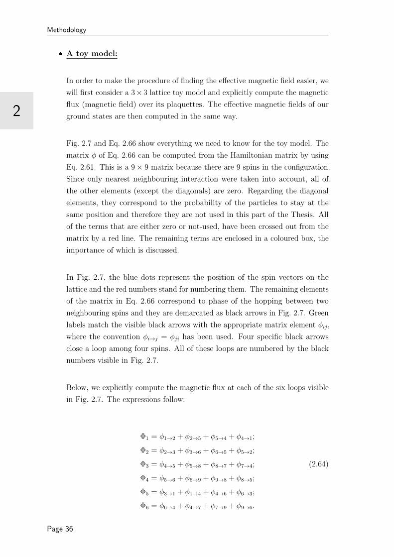
In order to make the procedure of finding the effective magnetic field easier, we

will first consider a 3× 3 lattice toy model and explicitly compute the magnetic

flux (magnetic field) over its plaquettes. The effective magnetic fields of our

ground states are then computed in the same way.

Fig. 2.7 and Eq. 2.66 show everything we need to know for the toy model. The

matrix φ of Eq. 2.66 can be computed from the Hamiltonian matrix by using

Eq. 2.61. This is a 9× 9 matrix because there are 9 spins in the configuration.

Since only nearest neighbouring interaction were taken into account, all of

the other elements (except the diagonals) are zero. Regarding the diagonal

elements, they correspond to the probability of the particles to stay at the

same position and therefore they are not used in this part of the Thesis. All

of the terms that are either zero or not-used, have been crossed out from the

matrix by a red line. The remaining terms are enclosed in a coloured box, the

importance of which is discussed.

In Fig. 2.7, the blue dots represent the position of the spin vectors on the

lattice and the red numbers stand for numbering them. The remaining elements

of the matrix in Eq. 2.66 correspond to phase of the hopping between two

neighbouring spins and they are demarcated as black arrows in Fig. 2.7. Green

labels match the visible black arrows with the appropriate matrix element φij,

where the convention φi→j = φji has been used. Four specific black arrows

close a loop among four spins. All of these loops are numbered by the black

numbers visible in Fig. 2.7.

Below, we explicitly compute the magnetic flux at each of the six loops visible

in Fig. 2.7. The expressions follow:

Φ1 = φ1→2 + φ2→5 + φ5→4 + φ4→1;

Φ2 = φ2→3 + φ3→6 + φ6→5 + φ5→2;

Φ3 = φ4→5 + φ5→8 + φ8→7 + φ7→4; (2.64)

Φ4 = φ5→6 + φ6→9 + φ9→8 + φ8→5;

Φ5 = φ3→1 + φ1→4 + φ4→6 + φ6→3;

Φ6 = φ6→4 + φ4→7 + φ7→9 + φ9→6.

Page 36

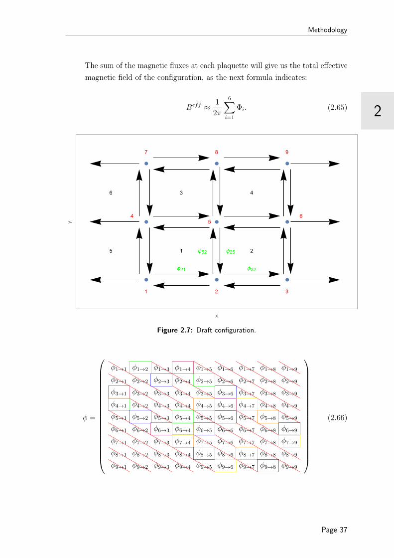
2

Methodology

The sum of the magnetic fluxes at each plaquette will give us the total effective

magnetic field of the configuration, as the next formula indicates:

Beff ≈ 1

2π

6∑i=1

Φi. (2.65)

1 2

3 4

5

6

1 2 3

45

6

7 8 9

ϕ21 ϕ32

ϕ52 ϕ25

x

y

Figure 2.7: Draft configuration.

φ =

φ1→1 φ1→2 φ1→3 φ1→4 φ1→5 φ1→6 φ1→7 φ1→8 φ1→9

φ2→1 φ2→2 φ2→3 φ2→4 φ2→5 φ2→6 φ2→7 φ2→8 φ2→9

φ3→1 φ3→2 φ3→3 φ3→4 φ3→5 φ3→6 φ3→7 φ3→8 φ3→9

φ4→1 φ4→2 φ4→3 φ4→4 φ4→5 φ4→6 φ4→7 φ4→8 φ4→9

φ5→1 φ5→2 φ5→3 φ5→4 φ5→5 φ5→6 φ5→7 φ5→8 φ5→9

φ6→1 φ6→2 φ6→3 φ6→4 φ6→5 φ6→6 φ6→7 φ6→8 φ6→9

φ7→1 φ7→2 φ7→3 φ7→4 φ7→5 φ7→6 φ7→7 φ7→8 φ7→9

φ8→1 φ8→2 φ8→3 φ8→4 φ8→5 φ8→6 φ8→7 φ8→8 φ8→9

φ9→1 φ9→2 φ9→3 φ9→4 φ9→5 φ9→6 φ9→7 φ9→8 φ9→9

(2.66)

Page 37

Methodology

2

The general case:

The toy model consists of 6 loops and therefore it is easy to explicitly compute

every term. The ground states though consist of more loops, which practically

makes listing of the magnetic fluxes impossible. This problem can be solved

by compactly writing all magnetic fluxes in one equation. This is not the end

of the story though since ferromagnetic and antiferromagnetic configurations

differ in the number of boundary conditions, hence the symbols δc,AFM and

δa,FM which were introduced in the previous subsection and more specifically

from Eq. 2.53 and Eq. 2.54 respectively, have to be used. As a consequence, the

index “i” has to bound itself at the number Lx (Ly − δc,FM). After considering

these restrictions, we end up with the following expression [33]1:

Φi,c =

φi→i+1 + φi+1→i+1+Lx + φi+1+Lx→i+Lx + φi+Lx→i if i 6= nLx

φi→i+1−Lx + φi+1−Lx→i+1 + φi+1→i+Lx + φi+Lx→i if i = nLx;

(2.67)

with i ∈ x | x ∈ N+ | x < LxLy due to the boundary conditions,

n ∈ x | x ∈ N+ | x < (Ly − δc,FM) and φjk to be the elements of the matrix

in Eq. 2.66.

Finally, the effective magnetic field will be given by the sum of the magnetic

fluxes, as Eq. 2.65 indicates. Hence, the compact form is written as:

Beffc ≈ 1

2π

Lx,c(Ly,c−δc,FM)∑i=1

Φi,c. (2.68)

2.6.3 Adiabatic Approximation

Alternatively, the adiabatic approximation provides us another way to extract the

effective magnetic filed of our lattices.

The basic idea is to map the existing problem, which is a magnon traversing a

spatially magnetic texture with constant amplitude, onto a problem, where the

magnon moves in a uniform Zeeman magnetic field, but instead feels an additional

1In [33] the expression for the total flux (at position (m,n)) reads: Φm,n = φxm,n + φym+1,n −φxm,n+1 − φym,n. The difference in the last two minus signs comes from the way the matrix elementsare computed and the orientation of their vectors. The two formulas are equivalent.

Page 38

2

Methodology

emergent electric and magnetic field [7]. The expression for the magnetic field is

given by:

bei =~2εi,j,kM ·

(∂jM× ∂kM

), (2.69)

where M = M/M the local magnetisation direction. The interested reader can

find more information regarding the derivation of this formula in the suggested

literature [7].

Since we are only interested in the z-direction of the emergent magnetic field, we

can plug i = z in Eq. 2.69 and after some simple algebra, we have:

bez = ~M ·(∂xM× ∂yM

). (2.70)

The interested reader can find more information in the following articles: [7, 37]

and [38, 39].

In order to find an expression that can be used to give us the emergent magnetic

field of our lattice, we have to perform some algebraic manipulations to Eq. 2.70.

Expanding the cross product by using the rule

a× b =

x y z

ax ay az

bx by bz

; (2.71)

allows us to write Eq. 2.69 as:

bez =

(∂My

∂x

∂Mz

∂y− ∂My

∂y

∂Mz

∂x

)Mx

−(∂Mx

∂x

∂Mz

∂y− ∂Mx

∂y

∂Mz

∂x

)My

+

(∂My

∂x

∂Mx

∂y− ∂Mx

∂y

∂My

∂x

)Mz. (2.72)

Eq. 2.72 has to be discretised in order to be used for our lattice. This can be done

by simply changing the derivatives with the difference of the magnetisation vectors

at the underlined direction. In such way we have:

Page 39

Methodology

2

bei,c = [(Myr −M

yi ) (M z

u −M zi )− (My

u −Myi ) (M z

r −M zi )]Mx

i

− [(Mxr −Mx

i ) (M zu −M z

i )− (Mxu −Mx

i ) (M zr −M z

i )]Myi

+ [(Mxr −Mx

i ) (Myu −M

yi )− (Mx

u −Mxi ) (My

r −Myi )]M z

i ; (2.73)

where i ∈ 1, LxLy and stands for the lattice points. r and u are the right and the

upper neighbour of i respectively. Finally, x, y, z stand for the Cartesian coordinates

of the magnetisation vector.

2.6.4 Final Expression

We have already seen that the transverse conductivity is given by Eq. 2.50 and that

the two terms that it consists of can be written, in terms of the parameters of the

configuration, as given by Eq. 2.55 and Eq. 2.68 respectively. In this subsection

we form the final expression for the transverse thermal conductivity into a single,

compact formula.

κxy,c ∝2Lx,cLy,c∑

α=Lx,cLy,c+1+δc,AFM

Lx,c(Ly,c−δc,FM)∑i=1

(1

eβ~ωα,c − 1

)bi,c. (2.74)

Alternatively, we can use Eq. 2.73 instead of Eq. 2.67.

Table 2.3 summarises the symbols in Eq. 2.74.

Symbol Stands for the... Valuec Index to distinguish the two different cases c ∈ FM,AFM

δc,FM , δc,AFM Kronecker’s delta of the configurations Eq, 2.54 and Eq. 2.53Lx,FM Length of the ferromagnetic configuration 16Ly,FM Width of the ferromagnetic configuration 16Lx,AFM Length of the antiferromagnetic configuration 32Ly,AFM Width of the antiferromagnetic configuration 32ωα,c Sorted eigenvalues of the Hamiltonian Numerical simulationbi,c Magnetic field at a specific closed loop Eq. 2.67 or Eq. 2.73

Table 2.3: Explanation of symbols present in Eq. 2.74.

Eq. 2.74 is all we need in order to compute the thermal transverse conductivity κxy,c.

Page 40

3

CHAPTER 3

Results

In the present Chapter, we present the result found using the theory and the

methodology discussed in Chapter 2. The figures were created using Mathematica

10 [40] as well as “TikZ” and the numerical procedure by using both a self-constructed

C++ code and the “Armadillo C++” external library [41]. The section is divided in

three subsections. The first one deals with ferromagnets and the second one with

antiferromagnets. Finally the third subsection compares the result of the previous

two. In the rest of this chapter “a” is the lattice constant and it is used to make

quantities dimensionless and ~ = 1.

3.1 Ferromagnets

The ground state is a 16× 16 skyrmionic lattice visible in Fig. 2.2. Below, we present

the dispersion of the system, the average magnon occupation per energy state, the

effective magnetic field distribution and some possible comparisons that can be done

by altering specific parameters. The mosaic of the chapter is completed by showing

the thermal dependency of the transverse conductivity.

3.1.1 Dispersion

In Fig. 3.1 the dispersion of the ground state of Hamiltonian 2.17 is depicted (the

coupling constants are in Table 2.1). To compare, we can see, in the appendix, the

dispersion of the Hamiltonian B.1 with ferromagnetic coupling J > 0 in the left part

of Fig. B.1.

Page 41

Results

3

0 50 100 150 200 2500

2

4

6

8

Mode

Ener

gy[|J|]

Ferromagnets

Figure 3.1: Dispersion of the system (ferromagnets).

3.1.2 Magnon Occupation

Since magnons are bosons, they will obey to the Bose-Einstein statistics (Eq. 2.51).

In Fig. 3.2 the average number of magnons in each state is depicted. Different colours

correspond to different values of β. As temperature decreases (β increases) less states

are occupied.

0 2 4 6 80

0.1

0.2

0.3

0.4

Energy [|J |]

Mag

non

Occ

upat

ion

Ferromagnets

β = 1 [1/|J |]β = 10 [1/|J |]

Figure 3.2: Occupation of magnons at each state (ferromagnets).

3.1.3 Effective Magnetic Field

In subsection 2.6 we discussed the equivalence of the Berry curvature and the ef-

fective magnetic field. Subsequently, in subsections 2.6.2 and 2.6.3 two methods to

Page 42

3

Results

numerically compute the effective magnetic field were analysed. In this subsection

we present the effective magnetic field found according to the previous analysis.

Fig. 3.3 illustrates the distribution of the effective magnetic field (or Berry curvature)

computed with the method of section 2.6.2. If we compare the effective magnetic field

distributions with the ground state in colour plot, as shown in Fig. 3.4, it becomes

clear that the presence of the skyrmion gives rise to large values of the magnetic

field.

2 4 6 8 10 12 14

5

10

xa

y a

Magnetic Field (J 6= 0, B 6= 0, D 6= 0)

0

0.2

0.4

0.6

0.8

Figure 3.3: Magnetic field distribution using Eq. 2.67 (ferromagnets).

0 2 4 6 8 10 12 140

5

10

15

xa

y a

Ground state

0.5

1

1.5

Figure 3.4: Colour plot of the ferromagnetic ground state.

We can also compute the effective magnetic field by using the adiabatic approximation

of section 2.6.3. The result is shown in Fig. 3.5. Again, this result is comparable to

Page 43

Results

3

the colour plot of the ground state (Fig. 3.4).

2 4 6 8 10 12 14

5

10

xa

y a

Magnetic Field (J 6= 0, D 6= 0, B 6= 0)

0

5 · 10−2

0.1

0.15

0.2

Figure 3.5: Magnetic field distribution using Eq. 2.73 (ferromagnets).

3.1.4 Comparisons

In this subsection, we theoretically investigate the behaviour of the effective magnetic

field for different values of the coupling constants of the Hamiltonian 2.17.

5 10 15

5

10

xa

y a

Magnetic Field (J 6= 0, D 6= 0, B 6= 0)

0

0.2

0.4

0.6

0.8

5 10 15

5

10

xa

y a

Magnetic Field (J = 0, D 6= 0, B 6= 0)

0

0.2

0.4

0.6

0.8

1

5 10 15

5

10

xa

y a

Magnetic Field (J 6= 0, D 6= 0, B 6= 0)

0

0.1

0.2

5 10 15

5

10

xa

y a

Magnetic Field (J 6= 0, D = 0, B 6= 0)

0

0.2

0.4

0.6

0.8

1

Figure 3.6: Distribution of the effective magnetic field for different values of Hamiltonian’scoupling constants (ferromagnets).

Page 44

3

Results

In Fig. 3.6 the magnetic field distributions for different values of couplings of the

Hamiltonian are illustrated. More specifically, the top left and the bottom left part

of the graph correspond to the full results explained in the previous section (the top

one was computed with the methodology discussed in section 2.6.2 and the bottom

one with the methodology of section 2.6.3). The top right part of Fig. 3.6 shows how

would the result of the magnetic field be, if there was no exchange interaction among

spins (J = 0). Finally, the bottom right part shows the hypothetical magnetic field

distribution of a Hamiltonian without Dzyaloshinskii-Moriya interaction (D = 0).

As it is obvious, both figures on the right part have no similarities with the initial

skyrmionic configuration, making them incorrect. This proves that the correct result

of the magnetic field distribution is only computed by using the Hamiltonian which

depends on all of the four terms described in section 2.2 and therefore only the left

part of the Figure is correct.

An alternative way to represent the distribution of the magnetic field for J 6= 0,

D 6= 0 and B 6= 0 in the Hamiltonian, is the one shown in Fig. 3.7. The height of

each point corresponds to the value of the effective magnetic field and the colour

just to make it easier recognisable.

Figure 3.7: The effective magnetic field in three-dimensions using Eq. 2.67.

Page 45

Results

30 2 4 6 8 10 12 14 16

0

2

4

6

8

10

12

14

xa

y a

Figure 3.8: Lines along which the values of the effective magnetic field in Fig. 3.9 and Fig. 3.10were taken.

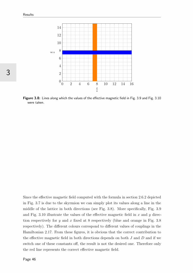
Since the effective magnetic field computed with the formula in section 2.6.2 depicted

in Fig. 3.7 is due to the skyrmion we can simply plot its values along a line in the

middle of the lattice in both directions (see Fig. 3.8). More specifically, Fig. 3.9

and Fig. 3.10 illustrate the values of the effective magnetic field in x and y direc-

tion respectively for y and x fixed at 8 respectively (blue and orange in Fig. 3.8

respectively). The different colours correspond to different values of couplings in the

Hamiltonian 2.17. From these figures, it is obvious that the correct contribution to

the effective magnetic field in both directions depends on both J and D and if we

switch one of these constants off, the result is not the desired one. Therefore only

the red line represents the correct effective magnetic field.

Page 46

3

Results

114 116 118 120 122 124 126 1280

1

2

3

4

5

6

i

b i

J 6= 0, D 6= 0, B 6= 0J 6= 0, D = 0, B 6= 0J = 0, D 6= 0, B 6= 0

Figure 3.9: Values of the effective magnetic field along the x-axis (y = 8). In this case113 ≤ i ≤ 128

72 104 136 1680

1

2

3

4

5

6

i

b i

J 6= 0, D 6= 0, B 6= 0J 6= 0, D = 0, B 6= 0J = 0, D 6= 0, B 6= 0

Figure 3.10: Values of the effective magnetic field along the y-axis (x = 8). In this casei ∈ kLx/2 | k ∈ N+ | k < Lx

Page 47

Results

3

3.1.5 Hall Conductivity

By using Eq. 2.74 it is easy to compute the values of the thermal transverse con-

ductivity for certain values of the inverse temperature β. However, temperature

T , as a physical quantity, is better understood and therefore Fig. 3.11 illustrates

the dependency of the transverse thermal conductivity on temperature. The blue

colour stands for the transverse thermal conductivity computed using the method

of section 2.6.2 (full result) whereas the light blue with the method discussed in

section 2.6.3 (adiabatic approximation).

For T = 0 there is no conductivity and therefore no Hall effect.

For T > 0 we can see a linear behaviour for both cases1.

0 0.2 0.4 0.6 0.8 10

1

2

3

4

5

6

7·104

TkB|J |

κxy

Ferromagnets

Full ResultAdiabatic Approximation

Figure 3.11: Transverse thermal conductivity as a function of temperature in ferromagnetscomputed with the two different methods.

1 A quadratic fit of the form a+ bx+ cx2 with a, b, c the unknown coefficients of the fit, will onlyimprove R2 in the 4th decimal place hence we can safely say that the data has linear behaviour.You can see R2 values for the linear and the quadratic fit in the following table.

Fit R2

Linear 0.999849Quadratic 0.999994

Page 48

3

Results

3.2 Antiferromagnets

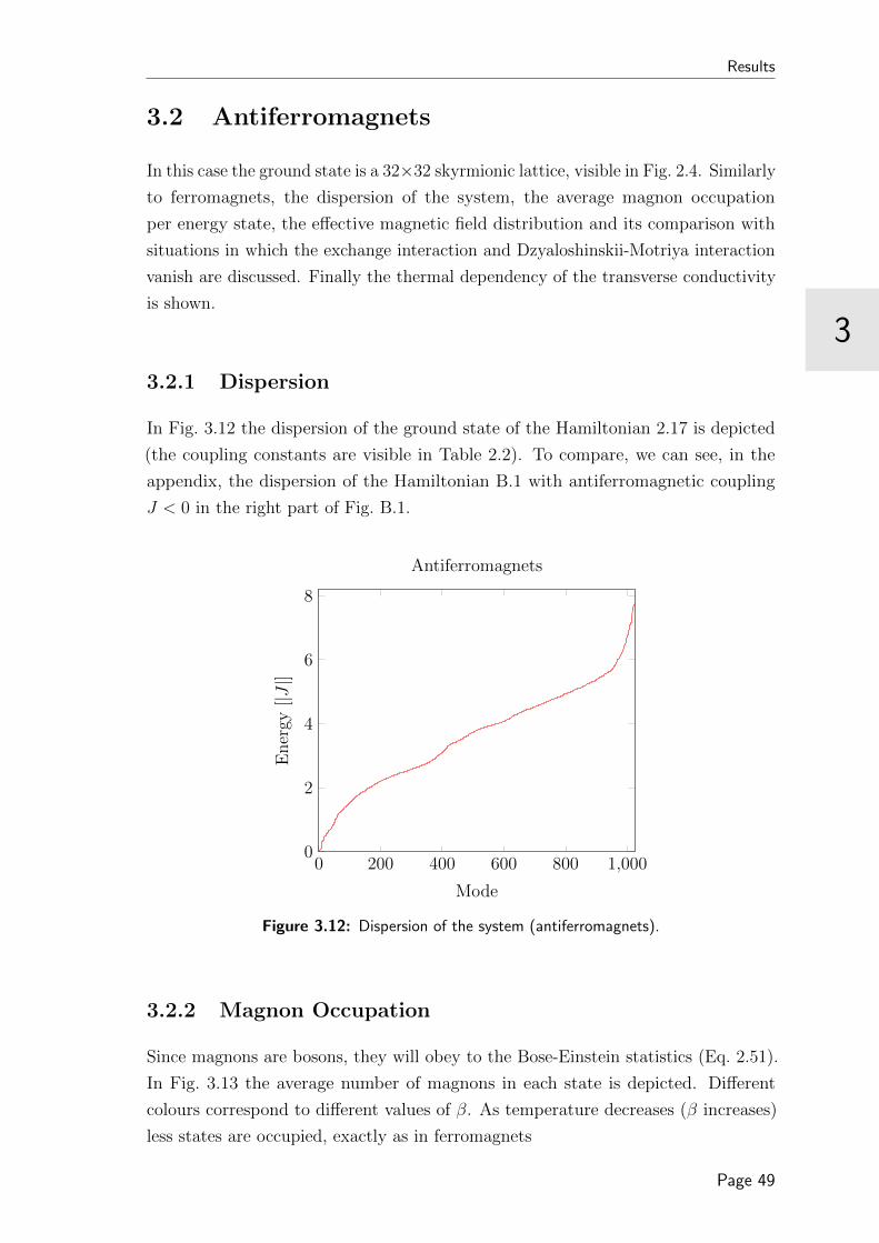
In this case the ground state is a 32×32 skyrmionic lattice, visible in Fig. 2.4. Similarly

to ferromagnets, the dispersion of the system, the average magnon occupation

per energy state, the effective magnetic field distribution and its comparison with

situations in which the exchange interaction and Dzyaloshinskii-Motriya interaction

vanish are discussed. Finally the thermal dependency of the transverse conductivity

is shown.

3.2.1 Dispersion

In Fig. 3.12 the dispersion of the ground state of the Hamiltonian 2.17 is depicted

(the coupling constants are visible in Table 2.2). To compare, we can see, in the

appendix, the dispersion of the Hamiltonian B.1 with antiferromagnetic coupling

J < 0 in the right part of Fig. B.1.

0 200 400 600 800 1,0000

2

4

6

8

Mode

Ener

gy[|J|]

Antiferromagnets

Figure 3.12: Dispersion of the system (antiferromagnets).

3.2.2 Magnon Occupation

Since magnons are bosons, they will obey to the Bose-Einstein statistics (Eq. 2.51).

In Fig. 3.13 the average number of magnons in each state is depicted. Different

colours correspond to different values of β. As temperature decreases (β increases)

less states are occupied, exactly as in ferromagnets

Page 49

Results

3

0 1 2 3 4 5 6 7 80

0.1

0.2

0.3

0.4

Energy [|J |]

Mag

non

Occ

upat

ion

Antiferromagnets

β = 1 [1/|J |]β = 10 [1/|J |]

Figure 3.13: Occupation of magnons at each state (antiferromagnets).

3.2.3 Effective Magnetic Field

Unlike the ferromagnetic case, the effective magnetic field distribution of the antifer-

romagnetic ground state is only computed using the method described in section

2.6.2. The result is shown in Fig. 3.14. Similarly to ferromagnets, the distribution of

the effective magnetic field is comparable to the colour plot of the antiferromagnetic

ground state, illustrated in Fig. 3.15, which shows that the large numbers of the

effective field are due to the skyrmions.

5 10 15 20 25 30

5

10

15

20

25

30

xa

y a

Magnetic Field (J 6= 0, D 6= 0, B 6= 0)

0.2

0.4

0.6

0.8

Figure 3.14: Magnetic field distribution using Eq. 2.67 (antiferromagnets).

Page 50

3

Results

5 10 15 20 25 30

5

10

15

20

25

30

xa

y a

Ground state

1

1.2

1.4

1.6

1.8

2

Figure 3.15: Colour plot of the antiferromagnetic ground state.

3.2.4 Comparisons

Similarly to ferromagnets, in this section we compare the results obtained after

computing the effective magnetic field using different couplings constants in the

Hamiltonian.

10 20 30

10

20

30

xa

y a

Magnetic Field (J 6= 0, D 6= 0, B 6= 0)

0.2

0.4

0.6

0.8

1

10 20 30

10

20

30

xa

y a

Magnetic Field (J = 0, D 6= 0, B 6= 0)

0.2

0.4

0.6

0.8

10 20 30

10

20

30

xa

y a

Magnetic Field (J 6= 0, D 6= 0, B 6= 0)

0

0.2

0.4

0.6

0.8

1

10 20 30

10

20

30

xa

y a

Ground state

1

1.2

1.4

1.6

1.8

2

Figure 3.16: Distribution of the effective magnetic field for different values of Hamiltonian’scoupling constants (antiferromagnets).

Page 51

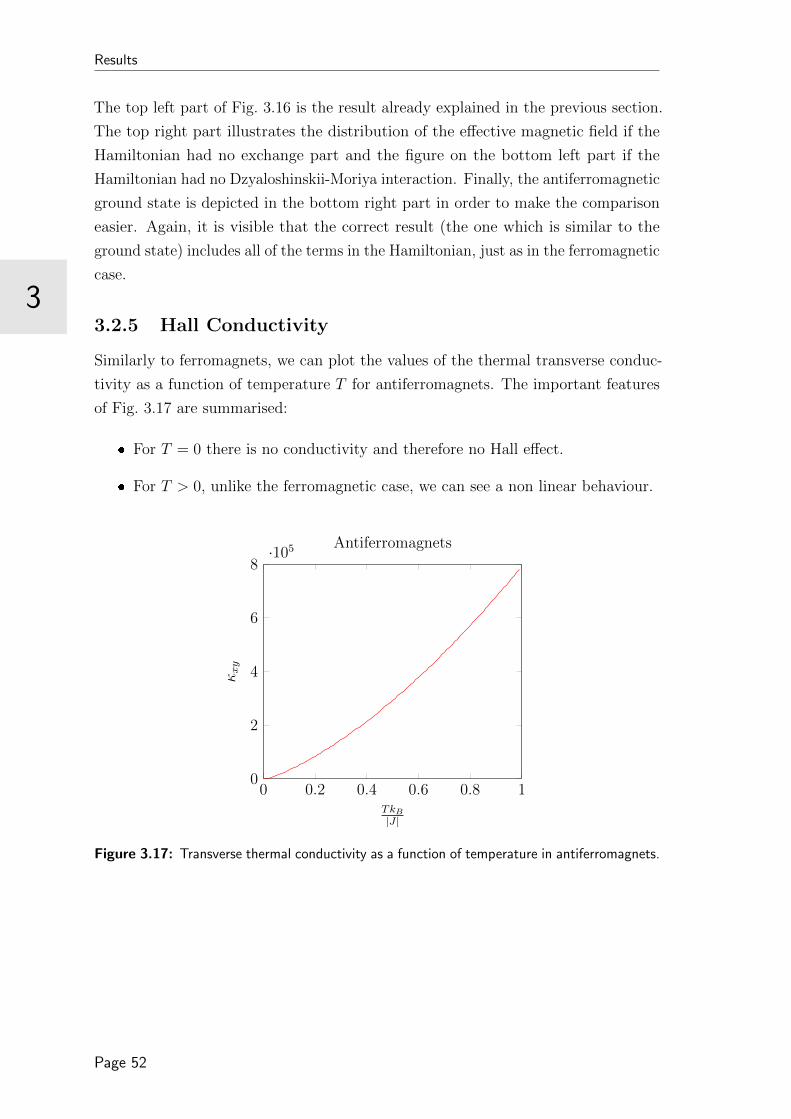
Results

3

The top left part of Fig. 3.16 is the result already explained in the previous section.

The top right part illustrates the distribution of the effective magnetic field if the

Hamiltonian had no exchange part and the figure on the bottom left part if the

Hamiltonian had no Dzyaloshinskii-Moriya interaction. Finally, the antiferromagnetic

ground state is depicted in the bottom right part in order to make the comparison

easier. Again, it is visible that the correct result (the one which is similar to the

ground state) includes all of the terms in the Hamiltonian, just as in the ferromagnetic

case.

3.2.5 Hall Conductivity

Similarly to ferromagnets, we can plot the values of the thermal transverse conduc-

tivity as a function of temperature T for antiferromagnets. The important features

of Fig. 3.17 are summarised:

For T = 0 there is no conductivity and therefore no Hall effect.

For T > 0, unlike the ferromagnetic case, we can see a non linear behaviour.

0 0.2 0.4 0.6 0.8 10

2

4

6

8·105

TkB|J |

κxy

Antiferromagnets

Figure 3.17: Transverse thermal conductivity as a function of temperature in antiferromagnets.

Page 52

3

Results

3.3 Comparisons and Conclusion

In this section we compare the results found in the section of ferromagnets with

these found in the section of antiferromagnets and give our final conclusion.

Comparing the magnon occupation of ferromagnets with that of the antiferromagnets,

we can stress that it does not depend on the character, hence for β = 1 the two curves

are identical as shown in Fig. 3.18. This is expected since the nature is bosonic in

both cases.

0 2 4 6 80

0.1

0.2

0.3

0.4

Energy [|J |]

Mag

non

Occ

upat

ion

β = 1

AFMFM

Figure 3.18: Comparison between the occupation number per state in FM and AFM for β = 1.

Probably the most important figure of the Thesis is the one which illustrates the

behaviour of the transverse thermal conductivity for both ferromagnetic and antifer-

romagnetic configurations in a single diagram. This can be seen in Fig. 3.19 and it

allows us to compare the two configurations.

Since the two configurations have to be stable, the freedom of picking a similar one,

in both cases is lost. As a consequence, the ground states not only differ in the size

but also in the number of skyrmions on them, making the comparison on the same ba-

sis almost impossible. This fact prevents us from saying which case is most profitable.

To sum up, by looking at Fig. 3.19 we conclude that the thermal conductivity of the

ferromagnetic lattice behaves linearly, whereas the thermal conductivity of the anti-

ferromagnetic lattice has a non-linear behaviour. Furthermore, the antiferromagnetic

lattice gives rise to larger absolute values of numbers of conductivities for all values

of temperature and therefore it explores a stronger thermal Hall effect. This is not a

comparison between the ferromagnetic and the antiferromagnetic case but between

Page 53

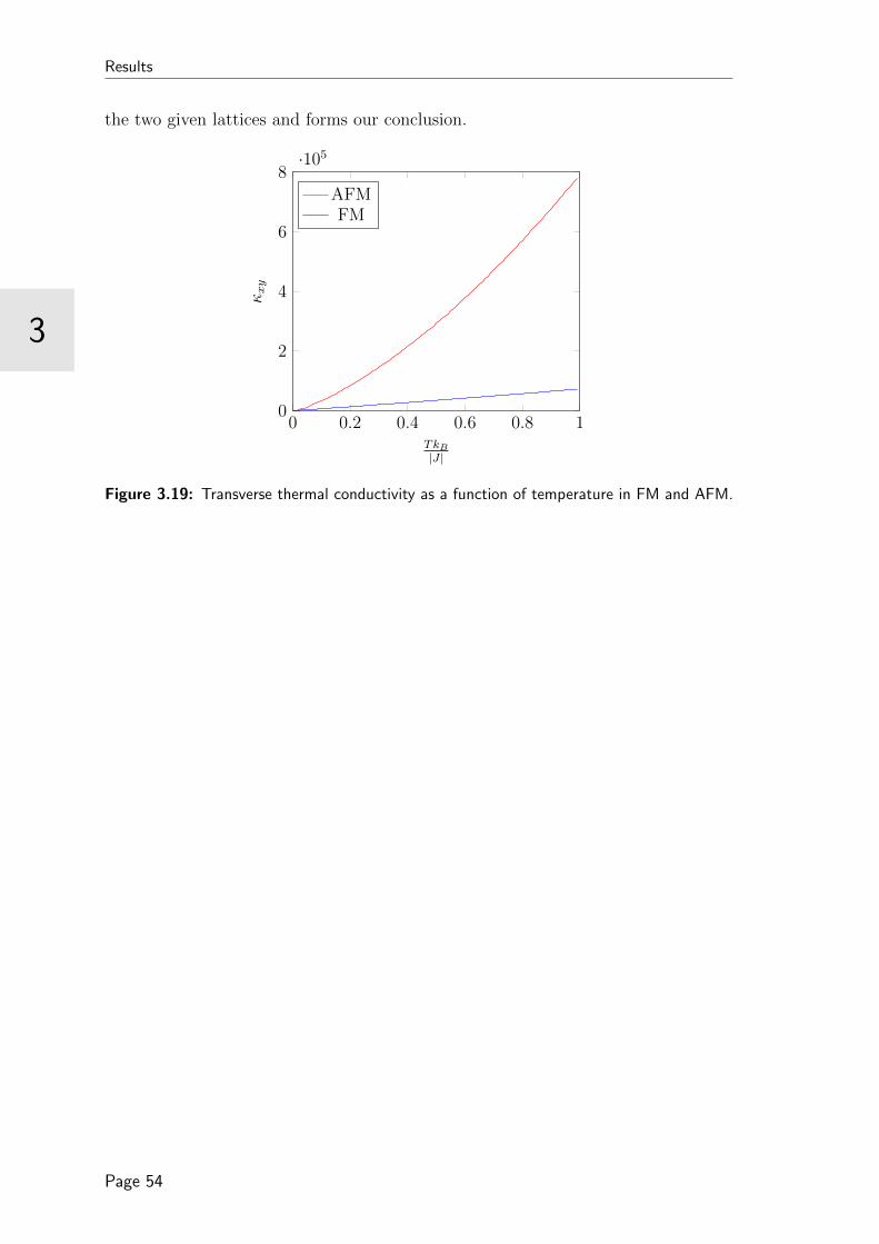
Results

3

the two given lattices and forms our conclusion.

0 0.2 0.4 0.6 0.8 10

2

4

6

8·105

TkB|J |

κxy

AFMFM

Figure 3.19: Transverse thermal conductivity as a function of temperature in FM and AFM.

Page 54

CHAPTER 4

Further Research

In this chapter, some suggestions for further research in the specific topic are ad-

dressed.

The transverse thermal conductivity (2.50) is related to some quantities (number

of magnons and effective magnetic field) that can be numerically computed

as a rule of proportionality instead of a strict mathematical equality. The

development of transport theory on numerical basis may directly relate these

quantities in a stricter mathematical way.

The investigation of the thermal Hall effect of magnons is limited to low

temperatures where interactions among spin waves and dissipation are negligible

phenomena. A complete description of the thermal Hall effect of magnons

though requires high-temperature analysis as well, for which the previously

mentioned phenomena cannot be neglected.

Since this topic is experimentally interesting as well, a further suggestion would

be to include in the model the coupling of the magnon system to the metallic

reservoirs, which is ignored in this Thesis.

Page 55

Further Research

Page 56

Appendices

Page 57

A

Ferromagnets and Antiferromagnets

As it is known, the quantum number of spin can only take two values for electrons

(s = 12

or s = −12). The former value corresponds to the situation “up”, whereas

the latter one to the situation “down”. Magnetic materials are characterised as

“ferromagnets” or “antiferromagnets” depending on the orientation of the spin of their

electrons. The left part of Fig. A.2 shows a perfect ferromagnet, in which all spins

point to the same direction. In reality there might be some small deviations and still

the material to be considered as a ferromagnet. Ferromagnets have a spontaneous

magnetisation even in the absence of an external field [21]. In the right part of

Fig. A.2 shows a perfect antiferromagnet. The orientation of spin strongly depends

on the temperature T . There is a critical temperature TC , the “Curie temperature”,

which specifies the magnetic properties of a material. Fig. A.1 summarizes the

dependence on the temperature of a magnetic material. It has to be mentioned that

the behaviour is similar to both ferromagnets and antiferromagnets.

Page 59

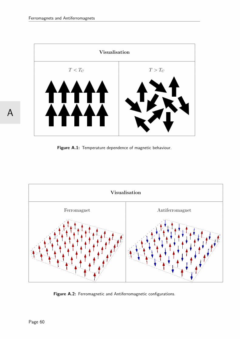
Ferromagnets and Antiferromagnets

A

Visualisation

T < TC T > TC

Figure A.1: Temperature dependence of magnetic behaviour.

Visualisation

Ferromagnet Antiferromagnet

Figure A.2: Ferromagnetic and Antiferromagnetic configurations.

Page 60

B

Magnon Dispersion Relation

The notion of magnons has already been introduced, however, a complete analysis

involves its dispersion relation as well, the derivation of which follows. In this Thesis

we are only interested in the behaviour of the dispersion relation and not in the

numerical value, hence any constant term will not been taken into account.

The Hamiltonian of a one-dimensional system reads:

H = −J∑〈i,j〉

SAi · SBj ; (B.1)

where A and B correspond to the different sublattices (the one consists of spins

pointing up and the other of spins pointing down).

Since only nearest neighbouring interactions are involved, the Hamiltonian B.1 can

be written as:

H = −J2

∑i

SAi · SBi+1 + SAi · SBi−1 + SBi · SAi+1 + SBi · SAi−1. (B.2)

Using that

SAi · SBj = Sx,Ai Sx,Bj + Sy,Ai Sy,Bj + Sz,Ai Sz,Bj , (B.3)

and that

Page 61

Magnon Dispersion Relation

B

SA,Bx =SA,B+ + SA,B−

2; (B.4)

SA,By =SA,B+ − SA,B−

2i,

we rewrite the Hamiltonian B.2 as:

H = −J2

∑i

[Sz,Ai Sz,Bi+1 + Sz,Ai Sz,Bi−1 + Sz,Bi Sz,Ai+1 + Sz,Bi Sz,Ai−1

+1

2

(S+,Ai S−,Bi+1 + S−,Ai S+,B

i+1 + S+,Ai S−,Bi−1 + S−,Ai S+,B

i−1

)+

1

2

(S+,Bi S−,Ai+1 + S−,Bi S+,A

i+1 + S+,Bi S−,Ai−1 + S−,Bi S+,A

i−1

) ]. (B.5)

In order to map the spin operators to creation and annihilation operators, we use

the Holstein-Primakoff transformations, the first term of the expansion of which are

given by:

S+,Ai '

√2Sai;

S−,Ai '√

2Sa†i ;

Sz,Ai ' Si − a†iai;

S+,Bj '

√2Sb†j;

S−,Bj '√

2Sbj;

Sz,Bj ' Sj − b†jbj. (B.6)

Plugging Eq. B.6 in Eq. B.5 and neglecting O (a4) terms we get:

H =∑iδ

JS(aibiδ + a†ib

†i+δ

)+ JS

(a†ia†i + b†i+δbi+δ

)+

+∑jδ

JS(bjaj+δ + b†ja

†j+δ

)+ JS

(b†jbj + a†i+δai+δ

)+

+ C, (B.7)

Page 62

B

Magnon Dispersion Relation

with δ to be the number of nearest neighbours (2 for one-dimensional system) and C

some unimportant numerical constant.

Hamiltonian B.7 can be further simplified if we transform it in momentum space k.

This can be done by defining the following relations.

ai =1√N

∑k

eik·xiak

bj =1√N

∑k

eik·xjbk

a†i =1√N

∑k

e−ik·xia†k

b†j =1√N

∑k

e−ik·xjb†k (B.8)

Substituting the Fourier transforms of Eq. B.8 in the Hamiltonian B.7 and after

some calculations, we get:

H =∑kα

JS cos kα(akb−k + a†kb

†−k

)+

+∑k

JS(a†kak + b†kbk

)+ C, (B.9)

with αl = xj − xi.

Since Hamiltonian B.9 includes terms with 2 creation (second term) or 2 annihilation

(first term) operators, the proper way to diagonilise it is by using the so called

Bogoliubov transformations. These transformations introduce some other operators

(ck and dk) in which the system has to be diagonal. The Bogoliubov relations are

defined as:

ck = ukak − vkb†−k;

dk = ukbk − vka†−k. (B.10)

Therefore, the inverse transformations are going to be:

Page 63

Magnon Dispersion Relation

B

ak = ukck + vkd†−k;

bk = ukdk + vkc†−k;

a−k = ukc−k + vkd†k;

b−k = ukd−k + vkc†k;

a†k = ukc†k + vkd−k;

b†k = ukd†k + vkc−k;

a†−k = ukc†−k + vkdk;

b†−k = ukd†−k + vkck. (B.11)

Hence, the Hamiltonian B.9 becomes:

H =∑kα

c†kck[2JSukvkγk + JS

(u2k + v2

k

)]+

+∑kα

d†kdk[2JSukvkγk + JS

(u2k + v2

k

)]+

+∑kα

(ckd−k + c†kd

†−k

) [JSγk

(u2k + v2

k

)+ 2JSukvk

]+

+ C, (B.12)

with γk =∑

α cos kα.

By definition, the coefficients of non diagonal terms (the last two terms in Eq. B.12)

have to be zero, hence the following constraint is fulfilled.

γk(u2k + v2

k

)+ 2ukvk = 0. (B.13)

Using that:

uk = cosh θk;

vk = sinh θk, (B.14)

Page 64

B

Magnon Dispersion Relation

we can write Eq. B.13 as:

γk(cosh2 θk + sinh2 θk

)+ 2 cosh θk sinh θk = 0. (B.15)

However, the following trigonometric relations hold:

cosh 2θk = cosh2 θk + sinh2 θk;

sinh 2θk = cosh θK sinh θk, (B.16)

therefore, we can write the condition (B.13) as:

γk = − tanh 2θk. (B.17)

Substituting Eq. B.17 in Hamiltonian B.12, we obtain:

H =∑k

ωk

(c†kck + d†kdk

)+ C, (B.18)

with ωk = JSz√

1− γ2k.

Hamiltonian B.18 is now diagonal. One can see two different types of operators

(ck/c†k and dk/d

†k), each of these annihilate/create a magnon with momentum k and

energy ωk. Hence, each state is degenerate.

Finally, a schematic representation of the ferromagnetic and the antiferromagnetic

dispersion of magnons can be seen in Fig. B.1.

Page 65

Magnon Dispersion Relation

B

Ferromagnet Antiferromagnet

0 20 40 60 80 100

0.0

0.5

1.0

1.5

2.0

Modes

ℏω

0 20 40 60 80 100

Modes

ℏω

Figure B.1: Ferromagnetic and Antiferromagnetic dispersion.

Page 66

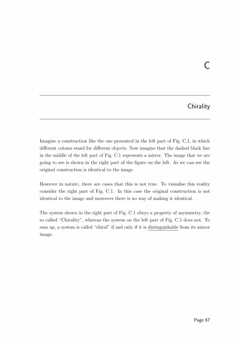
C

Chirality

Imagine a construction like the one presented in the left part of Fig. C.1, in which

different colours stand for different objects. Now imagine that the dashed black line

in the middle of the left part of Fig. C.1 represents a mirror. The image that we are

going to see is shown in the right part of the figure on the left. As we can see the

original construction is identical to the image.

However in nature, there are cases that this is not true. To visualise this reality

consider the right part of Fig. C.1. In this case the original construction is not

identical to the image and moreover there is no way of making it identical.

The system shown in the right part of Fig. C.1 obeys a property of asymmetry, the

so called “Chirality”, whereas the system on the left part of Fig. C.1 does not. To

sum up, a system is called “chiral” if and only if it is distinguishable from its mirror

image.

Page 67

Chirality

4

Non Chiral Chiral

Figure C.1: Chiral and non Chiral system.

Page 68

4

Chirality

References

[1] Y. Onose, T. Ideue, H. Katsura, Y. Shiomi, N. Nagaosa, and Y. Tokura, “Observationof the Magnon Hall Effect,” Science, vol. 329, no. 5989, pp. 297–299, 2010.

[2] S. Muhlbauer, B. Binz, F. Jonietz, C. Pfleiderer, A. Rosch, A. Neubauer, R. Georgii,and P. Boni, “Skyrmion lattice in a chiral magnet,” Science, vol. 323, no. 5916,pp. 915–919, 2009.

[3] R. Keesman, M. Raaijmakers, A. Baerends, G. Barkema, and R. Duine, “Skyrmionsin square-lattice Antiferromagnets,” arXiv preprint arXiv:1603.03688, 2016.

[4] “What are magnons?.” https://www.uni-muenster.de/Physik.AP/Demokritov/

en/Forschen/Forschungsschwerpunkte/mBECwam.html. Accessed: 2010-08-30.

[5] K. A. van Hoogdalem, Y. Tserkovnyak, and D. Loss, “Magnetic texture-inducedthermal hall effects,” Phys. Rev. B, vol. 87, p. 024402, Jan 2013.

[6] “Timezones.” http://militarytimechart.com/time-zones-explained/. Accessed:2010-09-30.

[7] K. Everschor-Sitte and M. Sitte, “Real-space berry phases: Skyrmion soccer,” Journalof Applied Physics, vol. 115, no. 17, p. 172602, 2014.

[8] D. J. Griffiths and E. G. Harris, “Introduction to quantum mechanics,” AmericanJournal of Physics, vol. 63, no. 8, pp. 767–768, 1995.

[9] M. I. Kaganov, Electrons, Photons, Magnons. Mir Publishers Moscow, 1981.

[10] M. G. Cottam, Linear and Nonlinear Spin Waves in Magnetic Films and Superlattices.World Scientific Publishing, 1994.

[11] S. A. Owerre, “Magnon hall effect in ab-stacked bilayer honeycomb quantum magnets,”Phys. Rev. B, vol. 94, p. 094405, Sep 2016.

[12] R. Resta, “Manifestations of Berry’s Phase in Molecules and Condensed Matter,”Journal of Physics: Condensed Matter, vol. 12, pp. R107+, Mar. 2000.

[13] G. Yin, Y. Li, L. Kong, R. K. Lake, C. L. Chien, and J. Zang, “Topological chargeanalysis of ultrafast single skyrmion creation,” Phys. Rev. B, vol. 93, p. 174403, May2016.

[14] M. Menzel, Non-collinear magnetic ground states observed in iron nanostructures oniridium surfaces. Verlag Dr. Hut, 2011.

[15] K. Uchida, J. Xiao, H. Adachi, J.-i. Ohe, S. Takahashi, J. Ieda, T. Ota, Y. Kajiwara,H. Umezawa, H. Kawai, et al., “Spin seebeck insulator,” Nature materials, vol. 9,no. 11, pp. 894–897, 2010.

[16] Y. Kajiwara, K. Harii, S. Takahashi, J. Ohe, K. Uchida, M. Mizuguchi, H. Umezawa,H. Kawai, K. Ando, K. Takanashi, et al., “Transmission of electrical signals by spin-wave interconversion in a magnetic insulator,” Nature, vol. 464, no. 7286, pp. 262–266,2010.

[17] F. Meier and D. Loss, “Magnetization transport and quantized spin conductance,”Phys. Rev. Lett., vol. 90, p. 167204, Apr 2003.

Page 69

Chirality

4

[18] J. Barker and O. A. Tretiakov, “Static and dynamical properties of antiferromagneticskyrmions in the presence of applied current and temperature,” Physical review letters,vol. 116, no. 14, p. 147203, 2016.

[19] B. Zimmermann, Calculation of the Dzyaloshinskii-Moriya Interaction in ultrathinmagnetic Films: Cr/W (110). PhD thesis, Diploma thesis, RWTH Aachen, 2010.

[20] G. Butenko, “Phenomenological theory of chiral states in magnets with dzyaloshinskii-moriya interactions,” 2012.

[21] S. Blundell, Magnetism in Condensed Matter (Oxford Master Series in Physics).Oxford University Press, USA, 1 ed., Dec. 2001.

[22] M. Bode, M. Heide, K. von Bergmann, P. Ferriani, S. Heinze, G. Bihlmayer, A. Kubet-zka, O. Pietzsch, S. Blugel, and R. Wiesendanger, “Chiral magnetic order at surfacesdriven by inversion asymmetry,” Nature, vol. 447, no. 7141, pp. 190–193.

[23] B. van Dijk, “Skyrmions and the dzyaloshinskii-moriya interaction,” 2015.

[24] R. Keesman, A. O. Leonov, P. van Dieten, S. Buhrandt, G. T. Barkema, L. Fritz, andR. A. Duine, “Degeneracies and fluctuations of neel skyrmions in confined geometries,”Phys. Rev. B, vol. 92, p. 134405, Oct 2015.

[25] A. Roldan-Molina, M. Santander, A. Nunez, and J. Fernandez-Rossier, “QuantumTheory of Spin Waves in Finite Chiral Spin Chains,” Physical Review B, vol. 89, no. 5,p. 054403, 2014.

[26] J. T. Haraldsen and R. S. Fishman, “Spin Rotation Technique for non-collinearMagnetic Systems: Application to the Generalized Villain Model,” Journal of Physics:Condensed Matter, vol. 21, no. 21, p. 216001, 2009.

[27] A. Roldan-Molina, M. Santander, A. Nunez, and J. Fernandez-Rossier, “Quantum Fluc-tuations Stabilize Skyrmion Textures,” Physical Review B, vol. 92, no. 24, p. 245436,2015.

[28] M.-w. Xiao, “Theory of Transformation for the Diagonalization of Quadratic Hamilto-nians,” arXiv preprint arXiv:0908.0787, 2009.

[29] J. Van Hemmen, “A Note on the Diagonalization of Quadratic Boson and FermionHamiltonians,” Zeitschrift fur Physik B Condensed Matter, vol. 38, no. 3, pp. 271–277,1980.

[30] J. Colpa, “Diagonalization of the quadratic boson hamiltonian,” Physica A: Statisticaland Theoretical Physics, vol. 93, pp. 327–353, Sept. 1978.

[31] R. Matsumoto and S. Murakami, “Theoretical prediction of a rotating magnon wavepacket in ferromagnets,” Phys. Rev. Lett., vol. 106, p. 197202, May 2011.

[32] V. K. Dugaev, P. Bruno, B. Canals, and C. Lacroix, “Berry phase of magnons intextured ferromagnets,” Phys. Rev. B, vol. 72, p. 024456, Jul 2005.

[33] M. Aidelsburger, Artificial gauge fields with ultracold atoms in optical lattices. Springer,2016.

[34] H. Katsura, N. Nagaosa, and P. A. Lee, “Theory of the thermal hall effect in quantummagnets,” Physical review letters, vol. 104, no. 6, p. 066403, 2010.

Page 70

4

Chirality

[35] J. Ibanez-Azpiroz, A. Eiguren, A. Bergara, G. Pettini, and M. Modugno, “Breakdownof the peierls substitution for the haldane model with ultracold atoms,” PhysicalReview A, vol. 90, no. 3, p. 033609, 2014.

[36] D. Sen and R. Chitra, “Large- U limit of a hubbard model in a magnetic field: Chiralspin interactions and paramagnetism,” Phys. Rev. B, vol. 51, pp. 1922–1925, Jan 1995.

[37] P. Bruno, V. Dugaev, and M. Taillefumier, “Topological hall effect and berry phase inmagnetic nanostructures,” Physical review letters, vol. 93, no. 9, p. 096806, 2004.

[38] T. Schulz, R. Ritz, A. Bauer, M. Halder, M. Wagner, C. Franz, C. Pfleiderer, K. Ever-schor, M. Garst, and A. Rosch, “Emergent electrodynamics of skyrmions in a chiralmagnet,” Nature Physics, vol. 8, no. 4, pp. 301–304, 2012.

[39] A. Neubauer, C. Pfleiderer, B. Binz, A. Rosch, R. Ritz, P. Niklowitz, and P. Boni,“Topological hall effect in the a phase of mnsi,” Physical review letters, vol. 102, no. 18,p. 186602, 2009.

[40] W. Research, “Mathematica 10.1,” 2015.

[41] C. Sanderson, “Armadillo: An Open Source C++ Linear Algebra Library for FastPrototyping and Computationally Intensive Experiments,” tech. rep., NICTA, Sept.2010.

Page 71