thermal effect on the underground power cables …
TRANSCRIPT
i
THERMAL EFFECT ON THE UNDERGROUND POWER CABLES
SAKTHIVEL SUBRAMANIAM
A project report submitted in partial fulfilment of the
requirements for the award of Master of Engineering (Electrical)
Faculty of Engineering and Science
University Tunku Abdul Rahman
April 2019
ii
1 DECLARATION
I hereby declare that this project report is based on my original work except for
citations and quotations which have been duly acknowledged. I also declare that it has
not been previously and concurrently submitted for any other degree or award at
UTAR or other institutions.
Signature :
Name : Sakthivel Subramaniam
ID No. : 17UEM05203
Date :
iii
1 APPROVAL FOR SUBMISSION
I certify that this project report entitled “THERMAL EFFECT ON THE
UNDERGROUND POWER CABLES” was prepared by SAKTHIVEL
SUBRAMANIAM has met the required standard for submission in partial fulfilment
of the requirements for the award of Master of Engineering (Electrical) at University
Tunku Abdul Rahman.
Approved by,
Signature :
Supervisor : Ir. Prof. Dr. Lim Yun Seng
Date :
Signature :
Co-Supervisor :
Date :

iv
The copyright of this report belongs to the author under the terms of the
copyright Act 1987 as qualified by Intellectual Property Policy of University Tunku
Abdul Rahman. Due acknowledgement shall always be made of the use of any
material contained in, or derived from, this report.
© 2019, Sakthivel Subramaniam. All right reserved.

v
Specially dedicated to
my beloved father, mother and my family members

vi
1 ACKNOWLEDGEMENTS
This project would not have been completed without the assistance of certain people
who were very kind and dedicated. First of all, it is a pleasure to thank my supervisor
Ir. Prof. Dr. Lim Yun Seng, for his kindness and endless assistance for this project.
Besides that, I am also thankful to everyone who all supported me, for I have
completed my project effectively and moreover on time.
Moreover, I would like to acknowledge to my classmates who helped me in
certain questions with fascinating ideas and tricks. With the combination of different
ideas of classmates, I have been able to tackle the obstacle easily. I would like to thank
my family who are my constant source of motivation, inspiration and supportive for
me to complete this final year project.
Last but not least, I would like to thank University Tunku Abdul Rahman
(UTAR) for providing a fabulous platform to learn in depth.

vii
1 ABSTRACT
“THERMAL EFFECT ON THE UNDERGROUND POWER CABLES”
In 33KV Single Core 1x630mm² XLPE Cable was investigated with
COMSOL software by changing the current carry capacity (ampacity) of the cable and
ambient ground temperature in Trefoil position. Result shows that the current makes
the operating temperature to rise and also the increased temperature will decrease the
current carry capacity of the cable. In matter of fact, the increased temperature causes
the current to reduce and consequently leading to increase in the current again. In terms
of the operating temperature and current it was achieved in stable values. Based on the
designed XLPE insulated cables, with different range of thermal conductivity of soil
was practically experienced. Basically, the ampacity of the cables will increase with
the higher thermal conductivity and also the ampacity will decrease with the lower
thermal conductivity. In fact, increased in the thermal conductivity will reduce the heat
production in the cables and also these will lead to reduction of the cables temperature.
Besides that, the flat position of the cables was laid next to each other and these causes
the temperature of the centre cable to increase due to heat transferred from the side
cables. In order to solve this, the current flow of the centre cable conductor was
decreased in order to reduce the operating temperature. Furthermore, the impact of
temperature distribution on the single core cable in two different burial depth which
are 0.5 meter and 1 meter was considered. It proves that the cables laid close to ground
surface had higher values of the operating cable conductor temperature and when the
single core cable are closer to the surface ground, the cable will receive more heat than
the single core cable buried in depth of 1 meter. Besides that, water has been used as
surrounding material of the cable by immersed in depth of 1 meter in order to study
and analyse the temperature distribution and current carrying capacity of the XLPE
insulated cables. In matter of fact, the operating temperature of the cables conductor is
higher than that the soil environment. This factor can be experienced because the heat
production from cables are slowly dispersed into the water surrounding environment
than the soil surrounding environment. In fact, the thermal conductivity of the water
can be one of the reason for the heating factor because it changes respectively with the
water ambient temperature. In the nutshell, running the power cables in the suitable
environment will extend the life expectancy, efficiency of the cables which provides
positive commitment to safety and economy of the connected power systems.

viii
TABLE OF CONTENTS
DECLARATION ii
APPROVAL FOR SUBMISSION iii
ACKNOWLEDGEMENT vi
ABSTRACT vii
TABLE OF CONTENTS viii
LIST OF FIGURES xi
LIST OF TABLES xvi
LIST OF SYMBOL/ ABBREVIATION xviii
LIST OF APPENDICES xx
CHAPTERS
1 INTRODUCTION 1
1.1 Background 1
1.2 Problem Statements 2
1.3 Aims and Objectives 3
1.4 Structure of the Research Report 4
2 LITERATURE REVIEW 5
2.1 Introduction 5
2.2 Cable Structures 5
2.2.1 Conductors 5
2.2.2 Conductor Shield and Insulation Shield (Semi-
conductive compound) 7
2.2.3 Insulation 8
2.2.5 Armoured Wires (Shield) 9
2.2.6 Insulation exterior (Jackets) 9
2.3 Software Used 10
2.3.1 COMSOL Multiphysics 10
ix
2.4 Summary 11
3 METHODOLOGY 12
3.1 Introduction 12
3.2 Modelling the Underground Power Cable 12
3.2.1 Using the COMSOL software 13
3.2.2 Designing the Geometry of the Underground Power
Cable (UPC) 15
3.2.3 Defining the Geometry of the Underground Power Cable
(UPC) 28
3.2.4 Selecting the Material Type for the Underground Power
Cable (UPC) 36
3.2.5 Meshing the ‘33kV Single core 630mm² XLPE Cable’
45
3.2.6 Adding Magnetic Field for the ‘33kV Single core
630mm² XLPE Cable’ 46
3.2.7 Adding the Thermal effect to the ‘33kV Single core
630mm² XLPE Cable’ 48
3.2.8 Adding the Multiphysics Couplings to the ‘33kV Single
core 630mm² XLPE Cable’ 50
3.2.8 Complete design of 33kV Single Core 630mm² Al XLPE
Cable by using COMSOL software. 54
3.3 Summary 56
4 RESULT AND DISCUSSSION 57
4.1 Introduction 57
4.2 Thermal effect on single-core cable 57
4.2.1 The Single Cable Buried Cable Under 0.5 meter Depth
58
4.2.2 The Result of Buried Cable under 1 meter Depth 60
4.2.3 Comparison of the result of the two cable depth of the
buried in 0.5 meter and 1 meter. 62
x
4.3 Effect of thermal conductivity of different types of soil on
underground power cables with current rating correction factors. 64
4.3.1 The Result of Operating Cable Conductor Temperature
using Different Soil Conditions with Correction Factor 67
4.3.2 Effect of thermal conductivity of different types of soil
on underground power cables without current rating correction
factors. 77
4.3.3 The discussion on the effect of thermal conductivity of
different types of soil on underground power cables with and
without current rating correction factors. 87
4.3.4 Effect of cable flat position on temperature distribution
90
4.3.5 Effect of Water on Cable 93
4.4 Summary 97
5 CONCLUSIONS AND RECOMMENDATIONS 98
5.1 Conclusion 98
5.2 Recommendations 99
6 APPENDICES 102

xi
1 LIST OF FIGURES
FIGURE TOPIC PAGE
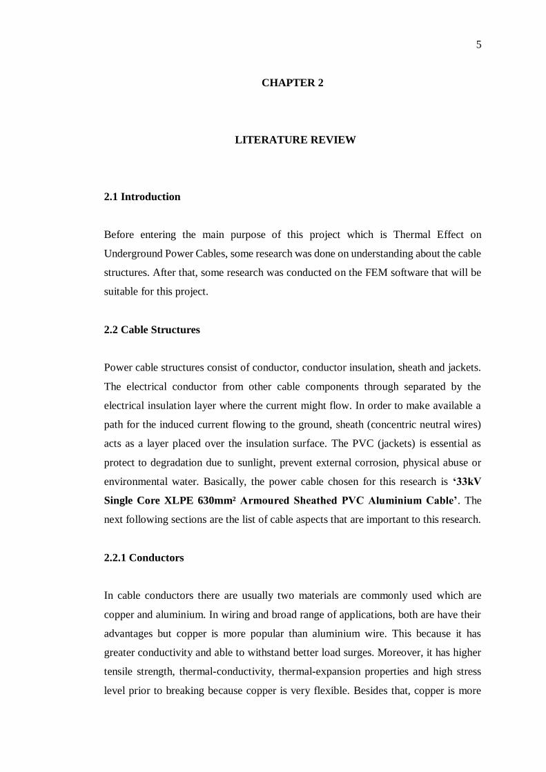
Figure 2.1: The Comparison of Aluminium and Copper 6
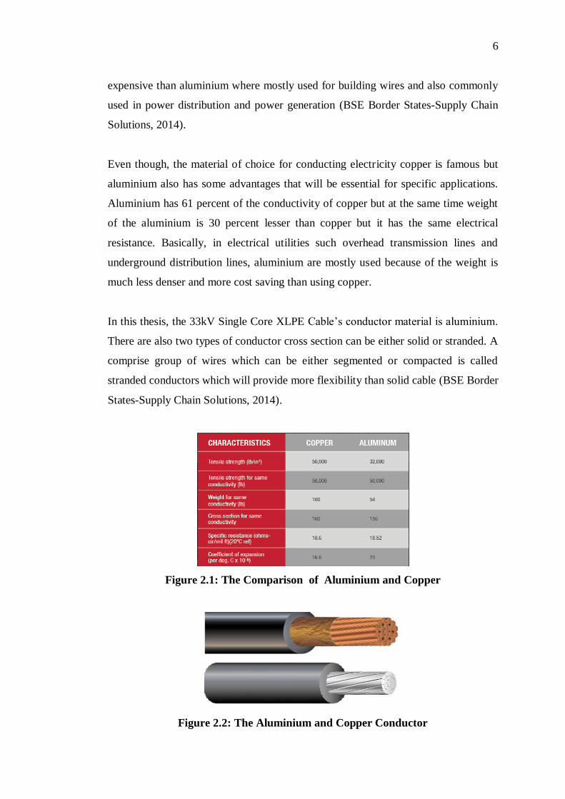
Figure 2.2: The Aluminium and Copper Conductor 6
Figure 2.3: Cable with and without Semi-conductive layer 7
Figure 2.4: The molecules structure of Polyethylene and Cross-linked Polyethylene. 8
Figure 2.5: The COMSOL Multiphysics Software 10
Figure 3.1: New Window 13
Figure 3.2: Blank model option 13
Figure 3.3: Blank model 14
Figure 3.4: Choosing the circle geometry for Semi-conductor. 14
Figure 3.5: Graphic window designed Semi-conductive layer of conductor 15
Figure 3.5: Choosing the circle geometry for Aluminium conductor. 16
Figure 3.6: Graphic window designed for Aluminium conductor 16
Figure 3.7: Choosing the circle geometry for Semi-conductive layer of insulation
(XLPE). 17
Figure 3.8: Graphic window designed for Semi-conductive layer of insulation (XLPE)
17
Figure 3.9: Choosing the circle geometry for PVC Insulation 18
Figure 3.10: Graphic window designed for PVC Insulation. 18
Figure 3.11: Choosing the circle geometry for Armoured wires 19
Figure 3.12: Graphic window designed for Armoured Wire 19
Figure 3.13: Choosing the Transform to copy Cable 1 20
Figure 3.14: Selecting the geometry of Cable 1 20
Figure 3.15: Storing the input geometric of Cable 1 21
Figure 3.16: Graphic window designed for Cable 2 21
Figure 3.17: Choosing the Transform to copy Cable 1 22
Figure 3.18: Selecting the geometry of Cable 1 22
Figure 3.19: Storing the input geometric of Cable 1 23
xii
Figure 3.19: Graphic window designed for Cable 3 23
Figure 3.20: Choosing the circle geometry for Electromagnetic field 24
Figure 3.21: The Graphic designed for Electromagnetic Field 24
Figure 3.22: Choosing the circle geometry for Surrounding Surface 25
Figure 3.23: The Graphic window designed of Surrounding Surface 25
Figure 3.24: The Graphic window for Whole Cable Geometry by using Union function.
26
Figure 3.25: Choosing the Explicit for Cables. 27
Figure 3.26: The Graphic window for the Definition of the Cables 27
Figure 3.27: Choosing the Explicit for Metal Internal. 28
Figure 3.28: The Graphic window for the Definition for the Metal Internal. 28
Figure 3.29: Choosing the Explicit for Aluminium Conductor. 29
Figure 3.30: The Graphic window for the Definition for the Metal Internal. 29
Figure 3.31: Choosing the Explicit for Insulation internal. 30
Figure 3.32: The Graphic window for the Definition for the Insulation Internal. 30
Figure 3.33: Choosing the Explicit for Semi-conductive compound. 31
Figure 3.34: The Graphic window for the Definition for the Semi-conductive
compound 31
Figure 3.35: Choosing the Explicit for PVC Insulation 32
Figure 3.36: The Graphic window for the Definition for the PVC Insulation 32
Figure 3.37: Choosing the Explicit function for Armoured Wires 33
Figure 3.38: The Graphic window for the Definition for the Armoured Wires 33
Figure 3.39: Choosing the Union function for Metal Internal and Armoured Wires 34
Figure 3.40: The Graphic window for the Metal Internal and Armoured Wires by using
Union 34
Figure 3.41: Choosing the Add Material for the cable 36
Figure 3.42: Selecting the Air material 36
Figure 3.43: The material Air was added in the design 36
Figure 3.44: The All materials are added 37
Figure 3.45: Selecting Air material to be assign 38
Figure 3.46: The Graphic window for the Air material assigned to surrounding of the
cable. 38
Figure 3.47: Selecting Soil or Water material to be assign 39
xiii
Figure 3.48: The Graphic window for the Soil or Water material assigned to
surrounding of the cable. 39
Figure 3.49: Selecting Polyvinyl Chloride (PVC) material to be assign 40
Figure 3.50: The Graphic window for Polyvinyl Chloride (PVC) assigned to the cable.
40
Figure 3.51: Selecting Semi-conductive compound material to be assign 41
Figure 3.52: The Graphic window for Semi-conductive compound assigned to the
cable. 41
Figure 3.53: Selecting Copper material to be assign 42
Figure 3.54: The Graphic window for Copper material assigned to the cable 42
Figure 3.55: Selecting Aluminium material to be assign 43
Figure 3.56: The Graphic window for Copper material assigned to the cable. 43
Figure 3.57: The Mesh setting for the cable 44
Figure 3.58: The Mesh Model of the ‘33kV Single core 630mm² XLPE Cable’ 44
Figure 3.59: Choosing the Add Physics for the cable 45
Figure 3.60: Selecting the Magnetic Fields for the cable 45
Figure 3.61: The Magnetic field was added to the cable 46
Figure 3.62: Choosing the Add Physics for the cable 47
Figure 3.63: Selecting the Heat Transfer in Solids for the cable 47
Figure 3.64: The Heat Transfer in Solid was added to the cable 48
Figure 3.65: Choosing the Multiphysics Coupling for the cable 49
Figure 3.66: The Electromagnetic Heating was added to the cable 49
Figure 3.67: The Temperature was added to the cable 50
Figure 3.68: The setting for Study 50
Figure 3.69: Selecting the Temperature (ht) 51
Figure 3.70: Choosing the result view 51
Figure 3.71: The Heat transfer on the cable 52
Figure 3.72: 33kV Single Core 630mm² Al XLPE Cable Structure 53
Figure 3.73: The Geometry of the ‘33kV Single Core 630mm² Al XLPE Cable’. 53
Figure 3.74: The Mesh Model of the ‘33kV Single core 630mm² XLPE Cable’ 54
Figure 3.75: The Thermal Effect on 33kV Single Core 630mm² Al XLPE Cable’ 54
Figure 4.1: The single cable buried in depth of 0.5 meter. 56

xiv
Figure 4.2: The operating temperature on underground power cables (UPC) buried in
depth of 0.5 meter (Zoom in view). 56
Figure 4.3: The operating temperature on underground power cables (UPC) buried in
depth of 0.5 meter (Zoom out view). 57
Figure 4.4: The single cable buried in depth of 1 meter. 59
Figure 4.5: The operating temperature on underground power cables (UPC) buried in
depth of 1 meter (Zoom in view). 59
Figure 4.6: The operating temperature on underground power cables (UPC) buried in
depth of 1 meter (Zoom in view). 60
Figure 4.7: The two cable depth of the buried in 0.5 meter and 1 meter 62
Figure 4.8: The operating temperature on underground power cables (UPC) buried in
depth of 1 meter in Tre-foil position (Zoom in view). 64
Figure 4.9: The operating temperature on underground power cables (UPC) under very
moist soil condition (Zoom in view). 68
Figure 4.10: The operating temperature on underground power cables (UPC) under
very moist soil condition (Zoom out view). 69
Figure 4.11: The operating temperature on underground power cables (UPC) under
moist soil condition (Zoom in view). 70
Figure 4.12: The operating temperature on underground power cables (UPC) under
moist soil condition (Zoom out view). 70
Figure 4.13: The operating temperature on underground power cables (UPC) under dry
soil condition (Zoom in view). 72
Figure 4.14: The operating cable conductor temperature (°C) at four different soil
conditions was tabulated into one table. 76
Figure 4.15: The Current carry capacity (Ampacity) of the cable at four different soil
conditions was tabulated into one table. 77
Figure 4.16: The operating temperature on underground power cables (UPC) under dry
soil condition (Zoom out view). 72
Figure 4.17: The operating temperature on underground power cables (UPC) under
very dry soil condition (Zoom in view). 74
Figure 4.18: The operating temperature on underground power cables (UPC) under
very dry soil condition (Zoom out view). 74
xv
Figure 4.19: The operating temperature on underground power cables (UPC) under
very moist soil condition (Zoom in view). 78
Figure 4.20: The operating temperature on underground power cables (UPC) under
very moist soil condition (Zoom out view). 78
Figure 4.21: The operating temperature on underground power cables (UPC) under
moist soil condition (Zoom in view). 81
Figure 4.22: The operating temperature on underground power cables (UPC) under
moist soil condition (Zoom out view). 81
Figure 4.23: The operating temperature on underground power cables (UPC) under dry
soil condition (Zoom in view). 83
Figure 4.24: The operating temperature on underground power cables (UPC) under dry
soil condition (Zoom out view). 83
Figure 4.25: The operating temperature on underground power cables (UPC) under
very dry soil condition (Zoom in view). 85
Figure 4.26: The operating temperature on underground power cables (UPC) under
very dry soil condition (Zoom out view). 85
Figure 4.27: The operating cable conductor temperature (°C) at four different soil
conditions without current rating correction factors 87
Figure 4.28: The operating temperature on underground power cables (UPC) in flat
position under dry soil condition. 91
Figure 4.29: The operating temperature on underground power cables (UPC) in flat
position after reducing the phase 2 cable ampacity under dry soil condition.
92
Figure 4.30: The operating temperature on underground power cables (UPC) in water
by changing the water temperature. 94
Figure 4.31: The Operating cable conductors’ temperature (°C) in water by changing
the water temperature. 95
Figure 4.32: The operating temperature on underground power cables (UPC) in water
by changing the ampacity. 96
Figure 4.33: The operating temperature on underground power cables (UPC) in water
by changing the ampacity. 96
xvi
1 LIST OF TABLES
TABLE TOPIC PAGE
Table 3.1: The Materials properties of the ‘33kV Single core 630mm² XLPE Cable”
35
Table 4.1: The Cable Conductor temperature of buried under 0.5 meter by changing
the ampacity. 58
Table 4.2: The Cable Conductor temperature of buried under 1 meter by changing the
ampacity. 61
Table 4.3: The two cable depth of the buried in 0.5 meter and 1 meter. 62
Table 4.4: The Soil Thermal Conductivity and Soil Thermal Resistivity Values 65
Table 4.5: The Ambient Ground Temperature (°C) 65
Table 4.6: Correction factor for ambient ground temperatures 66
Table 4.7: Correction factor for depth laying for direct buried cables 66
Table 4.8: Correction factor for soil thermal resistivity (K.m/W) 67
Table 4.9: The Cable Conductor Temperature (°C) of Very Moist Soil Condition
69
Table 4.10: The Cable Conductor Temperature (°C) of Moist Soil Condition
71
Table 4.11: The Cable Conductor Temperature (°C) of Dry Soil Condition
73
Table 4.12: The Cable Conductor Temperature (°C) of Very Dry Soil Condition 75
Table 4.13: The operating cable conductor temperature (°C) at four different soil
conditions was tabulated into one table. 76
Table 4.14: The current carry capacity (Ampacity) of the cable at four different soil
conditions was tabulated into one table. 77
Table 4.14: The Cable Conductor Temperature (°C) of Very Moist Soil Condition 80
Table 4.15: The Cable Conductor Temperature (°C) of Moist Soil Condition 84
xvii
Table 4.16: The Cable Conductor Temperature (°C) of Dry Soil Condition 84
Table 4.17: The Cable Conductor Temperature (°C) of Very Dry Soil Condition 86
Table 4.18: The operating cable conductor temperature (°C) at four different soil
conditions was tabulated into one table. 87
Table 4.19: The operating cable conductor temperature (°C) and the ampacity at
different soil conditions with correction factor 88
Table 4.20: The operating cable conductor temperature (°C) and the ampacity at
different soil conditions without correction factor 89
Table 4.21: The ampacity and operating cable conductors’ temperature (°C) of the
three cables. 93
Table 4.22: The operating cable conductors’ temperature (°C) in water by changing
the water temperature. 95
Table 4.23: The operating temperature on underground power cables (UPC) in water
by changing the ampacity. 96
xviii
LIST OF SYMBOLS/ ABBREVIATIONS
V Voltage
A Current
°C Temperature
K Thermal Conductivity
W/K*m Soil Thermal Conductivity
K*m/W Soil Thermal Resistivity
Rho Density
J/kg*k Heat Capacity
UPC Underground Power Cables
XLPE Cross-linked Polyethylene
PVC Polyvinyl Chloride
Dcon Diameter of conductor (Phase)
Tins Insulation thickness (Phase)
Dins Diameter over insulation (Phase)
Tscc Semi-conductive compound thickness (Phase)
Tarm Armor thickness (Cable)
Dcab Outer diameter of cable (Cable)
Acon Cross section of conductor (Phase)
Lcab Total length of cable (Cable)
f0 Operating frequency"
V0 Phase to ground voltage (Amplitude)
xix
I0 Rated current (Amplitude)
Pvc Thickness of outer sheath
Text External temperature
Tref Reference temperature (Metals)
Cu_alpha Resistivity temperature coefficient (Copper)
Cu_rho0 Reference resistivity,(Copper)
Scon Copper conductivity, 20 °C (Phase)
Sal Aluminium conductivity, 20 °C (Phase)
Rcon Aluminium DC resistance per phase, 20 °C (Analytic)
Rcu Copper DC resistance per phase, 20 °C (Analytic)
Exlpe XLPE relative permittivity (Phase)"

xx
LIST OF APPENDICES
APPENDIX TITLE PAGE
A XLPE Insulated Power & IEC Standards 104
(Central Cables Berhad (7169-A))

1
CHAPTER 1
1 INTRODUCTION
1.1 Background
One of the most important components in the power system is the power cable which
are used in the transmission (overhead lines) and distribution (underground lines).
Even though for power transmission lines are often chosen with overhead lines, for the
distribution site underground power cables are ideal to protect the operation in extreme
settlement areas, aesthetic appearance and favoured for ensuring safety of life. When
transmitted power range and voltage are increased, the basic structures of power cables
become complicated when they are designed to handle extra strength and heat build-
up. Furthermore, it is vital of existing systems at the peak capacity it requires
specification of maximum current carrying capacity of power cables and definition of
current carrying capacities of power cables are available through numerical or
analytical approaches. For this case, numerical analysis and among the other numerical
approaches, the most preferred methods is the finite element method (FEM) based on
the overall structure of the power cables (Kalenderli).
There is a solid connection between current conveying limit and operating temperature
of power cables. There will production of heat in the cable, when losses delivered by
voltage connected to a cable and current flowing through its conductor. The powerful
distribution of production of heat from the cable to the surrounding environment will
make the current conveying limits of a cables relies on it. This distribution will be
facing some problems because of the presence of high thermal resistances caused by
the insulating materials in cables and surrounding environment.
The maximum current value is characterized by the current capacity limit of power
cables where the cable conductor can convey constantly deprived of surpassing the
breaking point temperature value of the cable components, specifically not surpassing
that of protecting material. Along these lines, the temperature estimations of the cable
2
components during persistent process ought to be decided. Basically, the generated
heat inside the cable, numerical methods are applied for calculation of temperature
distribution in a cable and its surroundings environment. For this reason, using the
given conductor current, the conductor temperature was simulated using the software.
The simulation in thermal analysis are conducted by using geometry, material
information and boundary temperature conditions (Kalenderli).
1.2 Problem Statements
One of the important parts in the power system which is the high voltage power cable
is consistently involved in the increased temperature that will impact on the cable.
These will impact the cable properties and cause damages. In order to avoid this, this
research will be performed on study and analyse the effectiveness of using different
materials as backfill of the cable. After that, the laying of the cable under the soil by
choosing the best position of the cable will studied and analysed. Then, the operating
temperature of the cable will be measured by using the software with sufficient
information. Besides that, the operating cable conductor temperature with and without
current rating correction factor will be studied and analysed. Moreover, the operating
temperature of single cable conductor with different buried depth under the soil will
be studied and analysed. Finally, the operating temperature of the cable conductor
immersed in water will be studied and analysed.

3
1.3 Aims and Objectives
The objectives of conducting this research are listed below:
To study the cable specifications.
To study the temperature changes around the cable using Finite Element
Software called COMSOL software
To study, simulate, analyse and determine the effectiveness of using different
material as backfill of the cable.
To study, simulate, analyse and determine the laying position of the cable under
the soil in order to select the best position.
To study, simulate, analyse and determine the operating temperature of the
cable will be measured by using the software with sufficient information.
To study, simulate, analyse and determine the operating cable conductor
temperature with and without current rating correction factor.
To study, simulate, analyse and determine the operating temperature of single
power cable conductor with different buried depth under the soil.
To study, simulate, analyse and determine the operating temperature of the
cable conductor which will be immersed in water.
4
1.4 Structure of the Research Report
This report consists of five main chapters as briefly described below:
Chapter 1: Introduction
In this chapter, the background of this research, the problem statement as the purpose
of conducting this project and the aim and objective are specified.
Chapter 2: Literature Review
In this chapter, some research was done on the cable structures and the function of that
structures and also on the software used which COMSOL.
Chapter 3: Methodology
In this chapter, the modelling of the underground power cable, the geometry of the
cable, the material of the cable, the thermal effect of on the underground power cable
was designed.
Chapter 4: Results and Discussions
In this chapter, the effect of the operating temperature of the cable conductor with
different conditions using COMSOL was tabulated and discussed.
Chapter 5: Conclusion & Recommendations
In this chapter, concluding for the overall project purpose and recommendation for the
improvement that can be made from this project
5
CHAPTER 2
1 LITERATURE REVIEW
2.1 Introduction
Before entering the main purpose of this project which is Thermal Effect on
Underground Power Cables, some research was done on understanding about the cable
structures. After that, some research was conducted on the FEM software that will be
suitable for this project.
2.2 Cable Structures
Power cable structures consist of conductor, conductor insulation, sheath and jackets.
The electrical conductor from other cable components through separated by the
electrical insulation layer where the current might flow. In order to make available a
path for the induced current flowing to the ground, sheath (concentric neutral wires)
acts as a layer placed over the insulation surface. The PVC (jackets) is essential as
protect to degradation due to sunlight, prevent external corrosion, physical abuse or
environmental water. Basically, the power cable chosen for this research is ‘33kV
Single Core XLPE 630mm² Armoured Sheathed PVC Aluminium Cable’. The
next following sections are the list of cable aspects that are important to this research.
2.2.1 Conductors
In cable conductors there are usually two materials are commonly used which are
copper and aluminium. In wiring and broad range of applications, both are have their
advantages but copper is more popular than aluminium wire. This because it has
greater conductivity and able to withstand better load surges. Moreover, it has higher
tensile strength, thermal-conductivity, thermal-expansion properties and high stress
level prior to breaking because copper is very flexible. Besides that, copper is more
6
expensive than aluminium where mostly used for building wires and also commonly
used in power distribution and power generation (BSE Border States-Supply Chain
Solutions, 2014).
Even though, the material of choice for conducting electricity copper is famous but
aluminium also has some advantages that will be essential for specific applications.
Aluminium has 61 percent of the conductivity of copper but at the same time weight
of the aluminium is 30 percent lesser than copper but it has the same electrical
resistance. Basically, in electrical utilities such overhead transmission lines and
underground distribution lines, aluminium are mostly used because of the weight is
much less denser and more cost saving than using copper.
In this thesis, the 33kV Single Core XLPE Cable’s conductor material is aluminium.
There are also two types of conductor cross section can be either solid or stranded. A
comprise group of wires which can be either segmented or compacted is called
stranded conductors which will provide more flexibility than solid cable (BSE Border
States-Supply Chain Solutions, 2014).
Figure 2.1: The Comparison of Aluminium and Copper
Figure 2.2: The Aluminium and Copper Conductor

7
2.2.2 Conductor Shield and Insulation Shield (Semi-conductive compound)
The conductor shield is a layer between conductor and insulation (PVC, XLPE)
and the insulation shield is a layer between XLPE and Armoured wires which is
usually made of a semi-conductor material. The main purpose of conductor and
insulation shield is to maintain a homogeneously divergent electric field and to
surround the electric field within the cable core. Furthermore, it is basically to achieve
a radially symmetric electric field and “smoothest” out the surface irregularities of
conductor contour as well. Semi-conducting material of the conductor and insulation
doesn’t conduct electricity good enough to be conductor but will not hold back voltage.
The material are based on carbon black that is dispersed within a polymer matrix where
it must be sufficiently great enough to ensure a suitable and consistent conductivity.
Basically, to deliver a smooth interface between the conducting and insulating portions
of the cable, the integration must be optimized. The amount of regions of high
electrical stress also depends on the smooth surface in order to reduce the stress
(ANIXER, 2018).
Figure 2.3: Cable with and without Semi-conductive layer
8
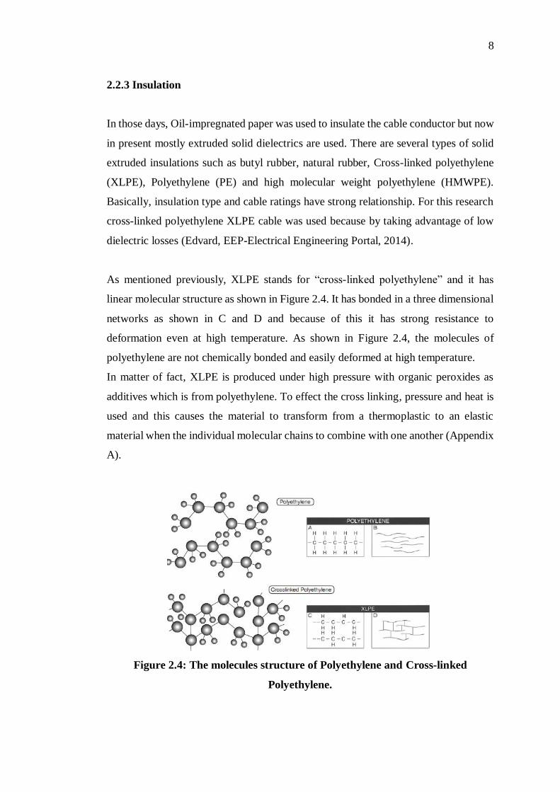
2.2.3 Insulation
In those days, Oil-impregnated paper was used to insulate the cable conductor but now
in present mostly extruded solid dielectrics are used. There are several types of solid
extruded insulations such as butyl rubber, natural rubber, Cross-linked polyethylene
(XLPE), Polyethylene (PE) and high molecular weight polyethylene (HMWPE).
Basically, insulation type and cable ratings have strong relationship. For this research
cross-linked polyethylene XLPE cable was used because by taking advantage of low
dielectric losses (Edvard, EEP-Electrical Engineering Portal, 2014).
As mentioned previously, XLPE stands for “cross-linked polyethylene” and it has
linear molecular structure as shown in Figure 2.4. It has bonded in a three dimensional
networks as shown in C and D and because of this it has strong resistance to
deformation even at high temperature. As shown in Figure 2.4, the molecules of
polyethylene are not chemically bonded and easily deformed at high temperature.
In matter of fact, XLPE is produced under high pressure with organic peroxides as
additives which is from polyethylene. To effect the cross linking, pressure and heat is
used and this causes the material to transform from a thermoplastic to an elastic
material when the individual molecular chains to combine with one another (Appendix
A).
Figure 2.4: The molecules structure of Polyethylene and Cross-linked
Polyethylene.

9
2.2.5 Armoured Wires (Shield)
Medium and high-voltage power cables mostly contain a shield layer (Armoured) of
copper or aluminium tapes or wires. The armoured wires is considered as protection
layer over the insulation (XLPE). The main function is to improve mechanical strength,
chemical corrosion, protect cables against moisture and physical abuse. This also
provide the return path for fault currents. Besides that, it must be connected to the
ground at least at one point because the induced current will flow on the armoured
wires. This will minimize the maximum current rating of the circuit and this current
will produce losses and heating. Moreover, it diverts any leakage current to ground by
equalizing electrical stress around the conductor. In order to confine the dielectric field
to the inside of this armoured wires (shield), the power cable must accomplished by
surrounding the assembly on insulation with a grounded as conducting medium. For
this research, armoured wires of copper material is used (Edvard, EEP-Electrical
Engineering Portal, 2014).
2.2.6 Insulation exterior (Jackets)
The insulation on the exterior layer of the cable is to protect the underlying conductor
against cable failures caused by any external electrical or mechanical damages. There
are several non-metallic materials can be used as exterior layer of the cable such as
Polyvinyl chloride (PVC), Polyethylene (PE) and Ethylene Propylene Rubber (EPR).
For this research, Polyvinyl chloride (PVC) insulated cables is used.
PVC is used in wide variety of applications where it is relatively low cost and combines
with plasticizers for electric cables.
PVC specification:
Has high tensile strength
Higher conductivity
Better flexibility
Ease of jointing
Basically, this material type of cable must take precaution not to overheat more than
90 °C, where it is suitable for a conductor up to 90 °C because it is a thermoplastic
material (ELAND CABLES, 2019).
10
2.3 Software Used
2.3.1 COMSOL Multiphysics
COMSOL Multiphysics is a cross-platform finite element analysis, solver and
multiphysics simulation software (Littmarck, 2015).
It provides an Integrated Development Environment (IDE) and unified
workflow for electrical, mechanical, fluid and chemical applications.
It allows conventional physics-based user interfaces and coupled system of
partial differential equation (PDEs).
To control the software externally, an Application Programming Interface (API)
for java and LiveLink for Matlab is used with the same API via the Method
Editor.
To develop independent domain-specific apps with custom user-interface,
comsol contains an App Builder.
To create custom physics-interfaces, comsol contains a Physics Builder from
the COMSOL Desktop with the same background as the built in physics
interfaces.
There are number of modules are available for COMSOL-Multiphysics which was
grouped according to the applications such as:
Electrical
Mechanical
Fluid
Chemical Multipurpose
Interfacing.
Figure 2.5: The COMSOL Multiphysics Software
11
2.4 Summary
In brief, the 33kV Single Core XLPE 630mm² Armoured Sheathed PVC Aluminium
Cable was chosen for this studies. Basically, the cable structures of these selected cable
are conductor, semi-conductive compound, the internal insulation, armoured wires and
external insulation. Firstly, the aluminium material are mostly used in the transmission
and distribution line because of the weight is much less denser and more cost saving
than using copper material. Second, the purpose of semi-conductive layer are to
achieve radially symmetric electric field and ‘smoothest’ out the surface irregularities
of XLPE insulation and conductor. Thirdly, XLPE insulation was used to insulate the
cable conductor and it has strong resistance to deformation even at high temperature.
Furthermore, the main function of armoured wires was to divert any leakage current
to ground by equalizing electrical stress around the conductor. Moreover, the PVC
insulation on the exterior layer of the cable will protect the underlying conductor
against cable failures caused by any external electrical or mechanical damages. This
are the cable structures that will be usually in the high voltage power cable
constructions. Besides that, the finite element method (FEM) with COMSOL software
contains number of modules which was grouped according to the applications such as
electrical, mechanical, fluid, chemical multipurpose and interfacing.
12
CHAPTER 3
1 METHODOLOGY
3.1 Introduction
In this chapter, the finite element method (FEM) with COMSOL software
was used as numerical method to study the thermal effect on the underground power
cable. This method is to define the problem with geometry, material and boundary
condition. To start off the geometry in this section, it is actually based on parameters.
In fact, most of the parameters are based upon on the international standards.
Furthermore, the cable type was chosen to model the geometry is ‘33kV Single core
630mm² Al XLPE Cable’. The parameters of this cable based on the ‘Central Cable
Berhad’ specification (Appendix A).
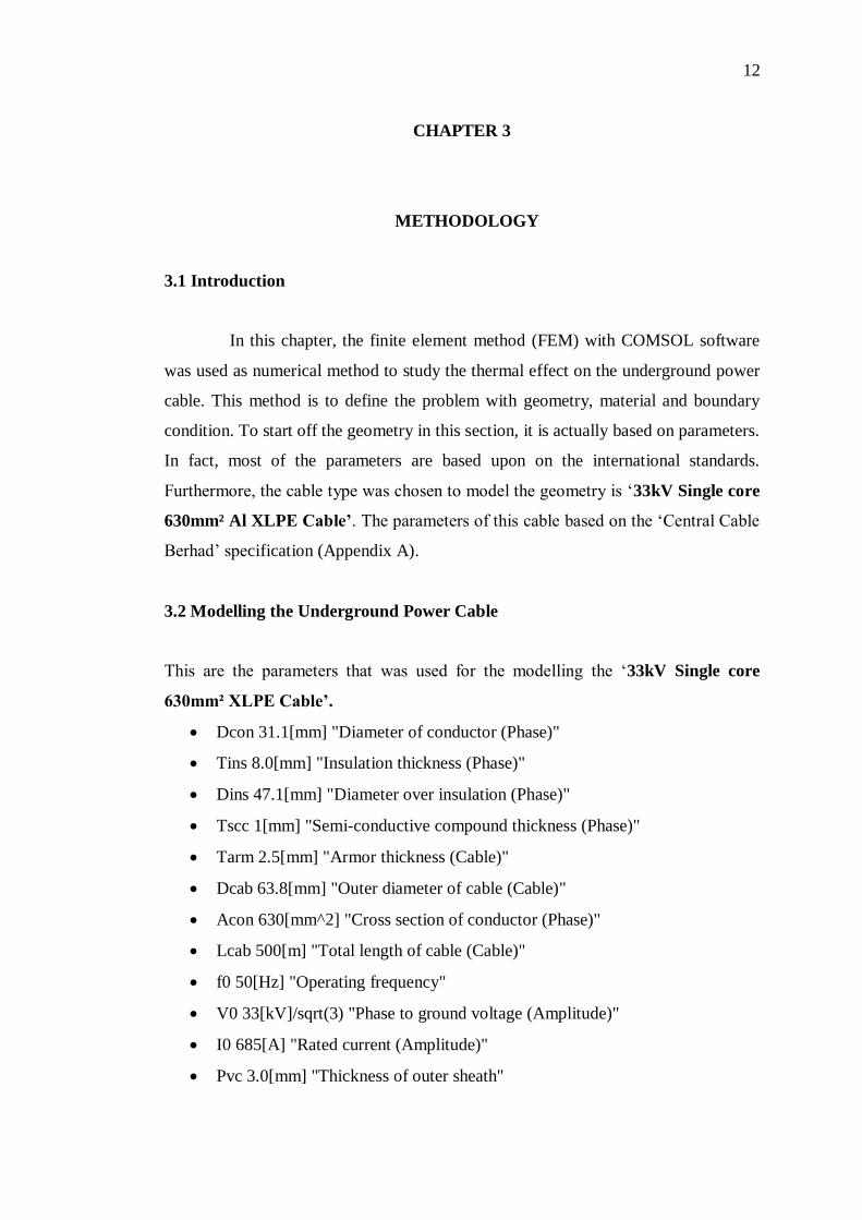
3.2 Modelling the Underground Power Cable
This are the parameters that was used for the modelling the ‘33kV Single core
630mm² XLPE Cable’.
Dcon 31.1[mm] "Diameter of conductor (Phase)"
Tins 8.0[mm] "Insulation thickness (Phase)"
Dins 47.1[mm] "Diameter over insulation (Phase)"
Tscc 1[mm] "Semi-conductive compound thickness (Phase)"
Tarm 2.5[mm] "Armor thickness (Cable)"
Dcab 63.8[mm] "Outer diameter of cable (Cable)"
Acon 630[mm^2] "Cross section of conductor (Phase)"
Lcab 500[m] "Total length of cable (Cable)"
f0 50[Hz] "Operating frequency"
V0 33[kV]/sqrt(3) "Phase to ground voltage (Amplitude)"
I0 685[A] "Rated current (Amplitude)"
Pvc 3.0[mm] "Thickness of outer sheath"
13
Text 35[degC] "External temperature
Tref 90[degC] "Reference temperature (Metals)"
Cu_alpha 3.9e-3[1/K] "Resistivity temperature coefficient (Copper)"
Cu_rho0 1/Scon "Reference resistivity,(Copper)"
Scon 5.96e7[S/m] "Copper conductivity, 20 °C (Phase)"
Sal 3.77e7[S/m] "Aluminium conductivity, 20 °C (Phase)"
Rcon 1/Acon/Sal "Aluminium DC resistance per phase, 20 °C (Analytic)"
Rcu 1/Acu/Scon "Copper DC resistance per phase, 20 °C (Analytic)"
Exlpe 2.5 "XLPE relative permittivity, from IEC 60287 (Phase)"
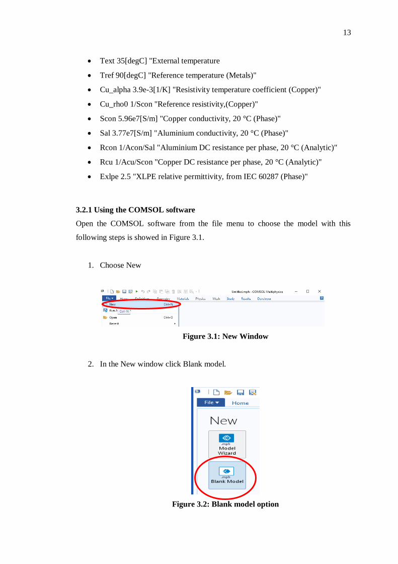
3.2.1 Using the COMSOL software
Open the COMSOL software from the file menu to choose the model with this
following steps is showed in Figure 3.1.
1. Choose New
Figure 3.1: New Window
2. In the New window click Blank model.
Figure 3.2: Blank model option
14
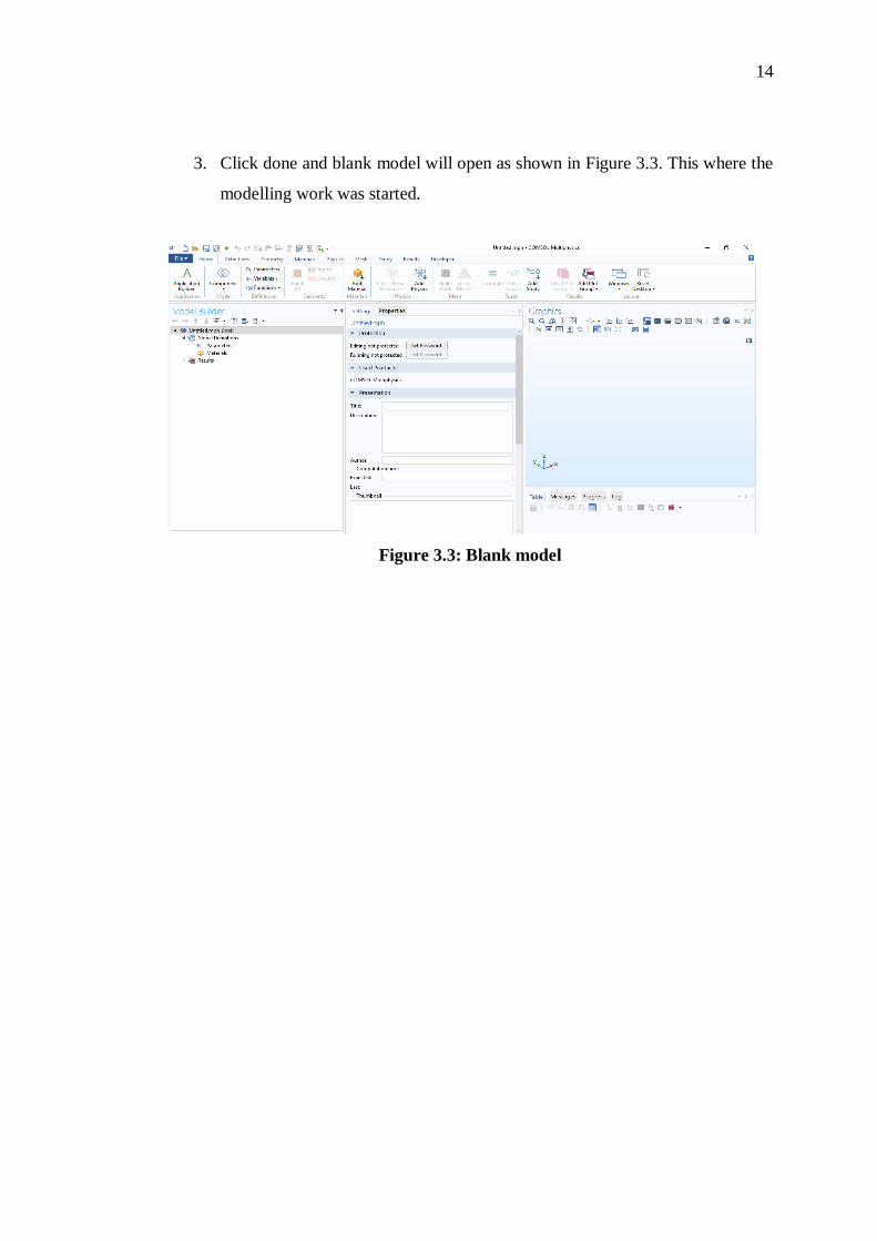
3. Click done and blank model will open as shown in Figure 3.3. This where the
modelling work was started.
Figure 3.3: Blank model
15
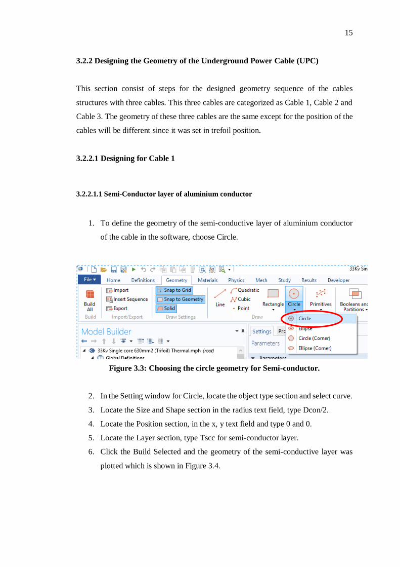
3.2.2 Designing the Geometry of the Underground Power Cable (UPC)
This section consist of steps for the designed geometry sequence of the cables
structures with three cables. This three cables are categorized as Cable 1, Cable 2 and
Cable 3. The geometry of these three cables are the same except for the position of the
cables will be different since it was set in trefoil position.
3.2.2.1 Designing for Cable 1
3.2.2.1.1 Semi-Conductor layer of aluminium conductor
1. To define the geometry of the semi-conductive layer of aluminium conductor
of the cable in the software, choose Circle.
Figure 3.3: Choosing the circle geometry for Semi-conductor.
2. In the Setting window for Circle, locate the object type section and select curve.
3. Locate the Size and Shape section in the radius text field, type Dcon/2.
4. Locate the Position section, in the x, y text field and type 0 and 0.
5. Locate the Layer section, type Tscc for semi-conductor layer.
6. Click the Build Selected and the geometry of the semi-conductive layer was
plotted which is shown in Figure 3.4.

16
Figure 3.4: Graphic window designed Semi-conductive layer of conductor
17
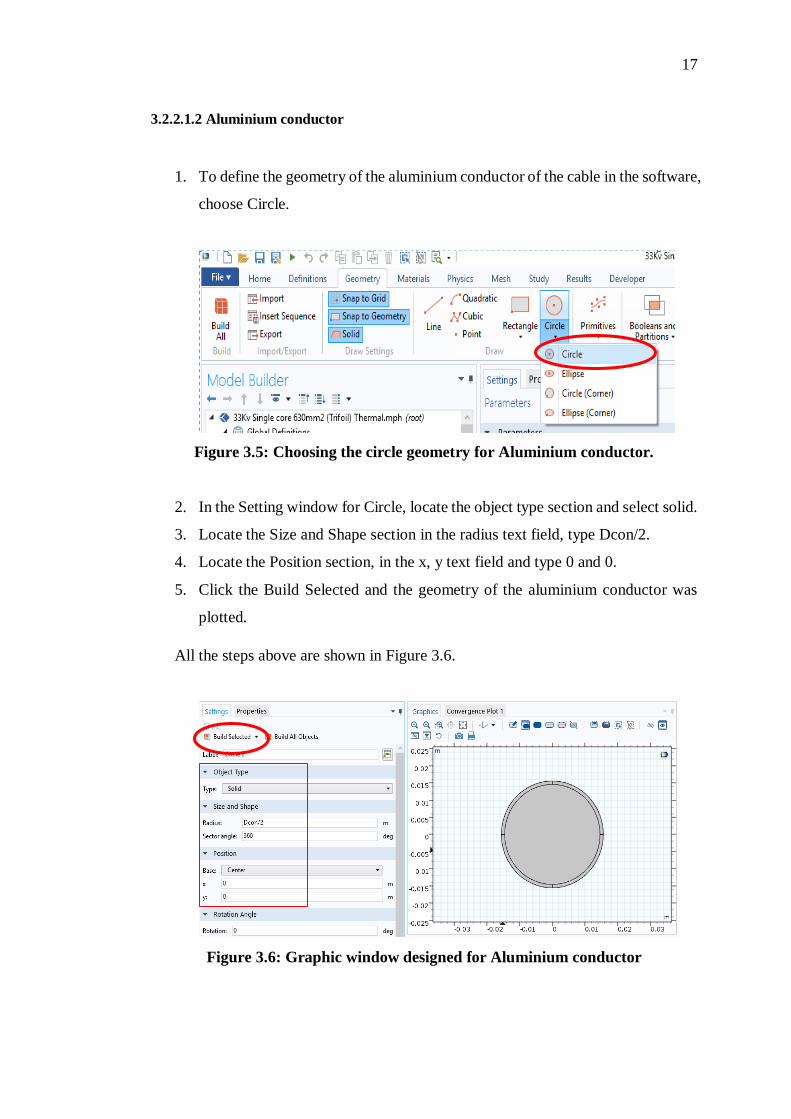
3.2.2.1.2 Aluminium conductor
1. To define the geometry of the aluminium conductor of the cable in the software,
choose Circle.
Figure 3.5: Choosing the circle geometry for Aluminium conductor.
2. In the Setting window for Circle, locate the object type section and select solid.
3. Locate the Size and Shape section in the radius text field, type Dcon/2.
4. Locate the Position section, in the x, y text field and type 0 and 0.
5. Click the Build Selected and the geometry of the aluminium conductor was
plotted.
All the steps above are shown in Figure 3.6.
Figure 3.6: Graphic window designed for Aluminium conductor

18
3.2.2.1.3 Semi-Conductive layer of insulation (XLPE)
1. To define the geometry of the semi-conductive layer of insulation (XLPE) of
the cable in the software, choose Circle.
Figure 3.7: Choosing the circle geometry for Semi-conductive layer of insulation
(XLPE).
2. In the Setting window for Circle, locate the object type section and select curve.
3. Locate the Size and Shape section in the radius text field, type Dins/2.
4. Locate the Position section, in the x, y text field and type 0 and 0.
5. Locate the Layer section, type Tscc for semi-conductor layer.
6. Click the Build Selected and the geometry of the Semi-conductor layer of
insulation (XLPE) was plotted.
All the steps above are shown in Figure 3.8.
Figure 3.8: Graphic window designed for Semi-conductive layer of insulation
(XLPE)
19
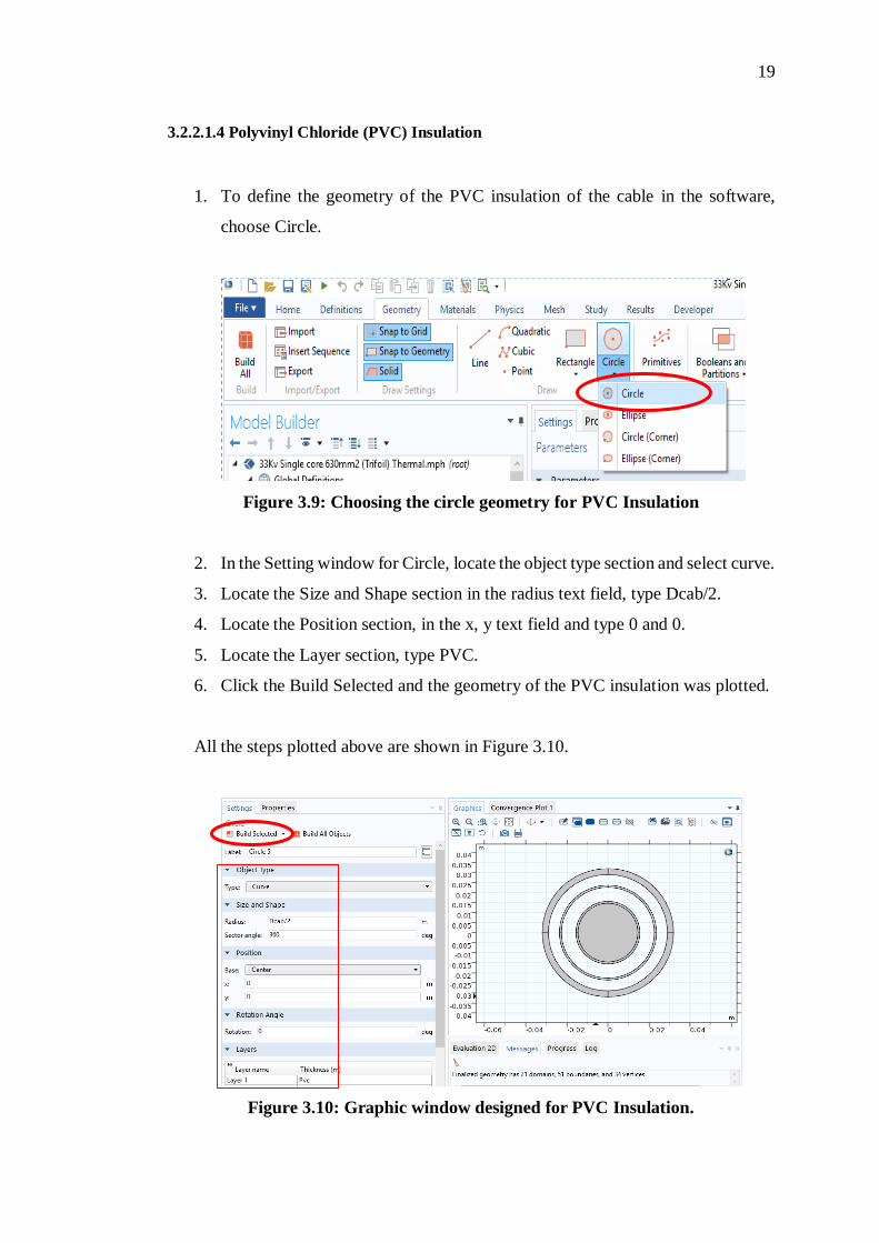
3.2.2.1.4 Polyvinyl Chloride (PVC) Insulation
1. To define the geometry of the PVC insulation of the cable in the software,
choose Circle.
Figure 3.9: Choosing the circle geometry for PVC Insulation
2. In the Setting window for Circle, locate the object type section and select curve.
3. Locate the Size and Shape section in the radius text field, type Dcab/2.
4. Locate the Position section, in the x, y text field and type 0 and 0.
5. Locate the Layer section, type PVC.
6. Click the Build Selected and the geometry of the PVC insulation was plotted.
All the steps plotted above are shown in Figure 3.10.
Figure 3.10: Graphic window designed for PVC Insulation.
20
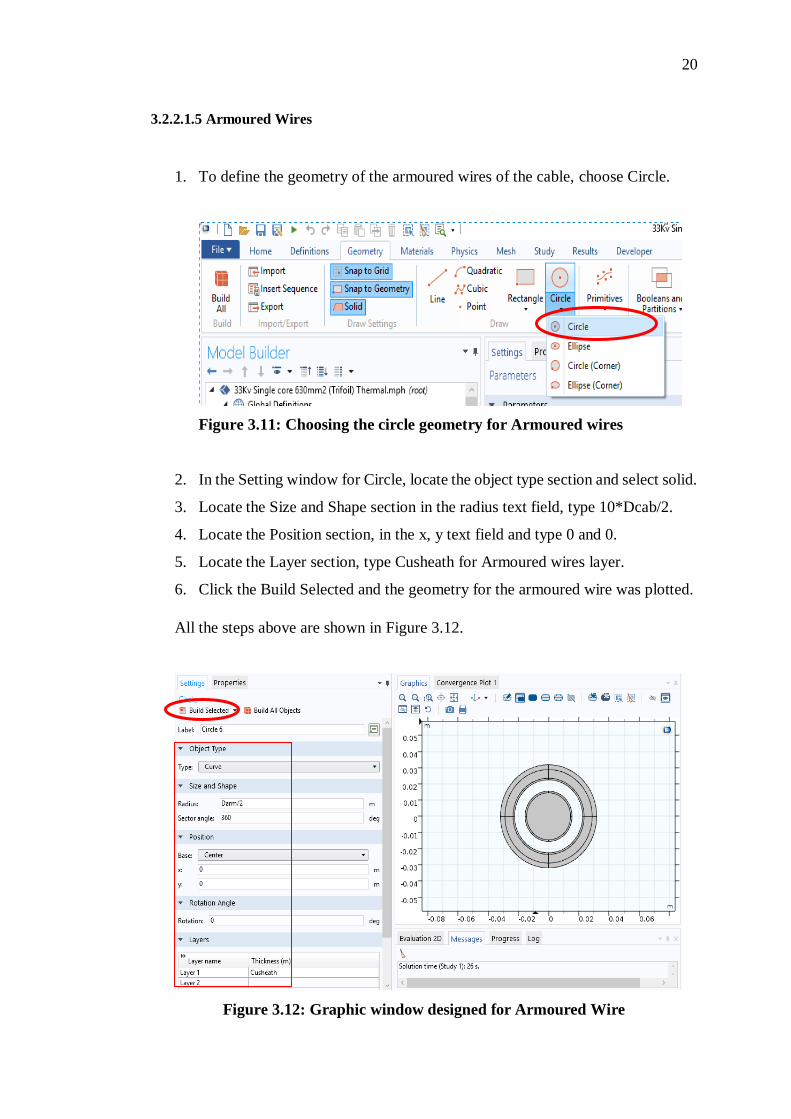
3.2.2.1.5 Armoured Wires
1. To define the geometry of the armoured wires of the cable, choose Circle.
Figure 3.11: Choosing the circle geometry for Armoured wires
2. In the Setting window for Circle, locate the object type section and select solid.
3. Locate the Size and Shape section in the radius text field, type 10*Dcab/2.
4. Locate the Position section, in the x, y text field and type 0 and 0.
5. Locate the Layer section, type Cusheath for Armoured wires layer.
6. Click the Build Selected and the geometry for the armoured wire was plotted.
All the steps above are shown in Figure 3.12.
Figure 3.12: Graphic window designed for Armoured Wire
21
3.2.2.2 Designing for Cable 2
Basically to design the cable 2 doesn’t need to follow the same steps as cable 1 where
the copy method can used.
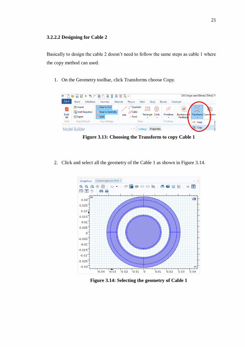
1. On the Geometry toolbar, click Transforms choose Copy.
Figure 3.13: Choosing the Transform to copy Cable 1
2. Click and select all the geometry of the Cable 1 as shown in Figure 3.14.
Figure 3.14: Selecting the geometry of Cable 1
22
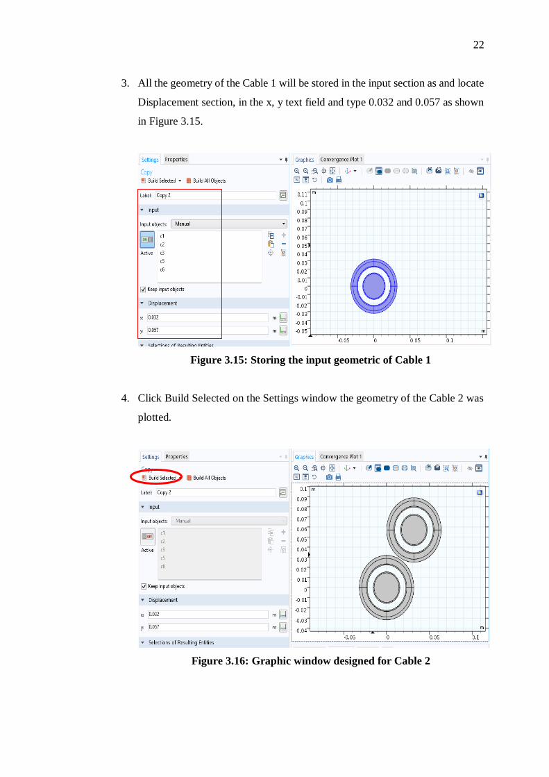
3. All the geometry of the Cable 1 will be stored in the input section as and locate
Displacement section, in the x, y text field and type 0.032 and 0.057 as shown
in Figure 3.15.
Figure 3.15: Storing the input geometric of Cable 1
4. Click Build Selected on the Settings window the geometry of the Cable 2 was
plotted.
Figure 3.16: Graphic window designed for Cable 2
23
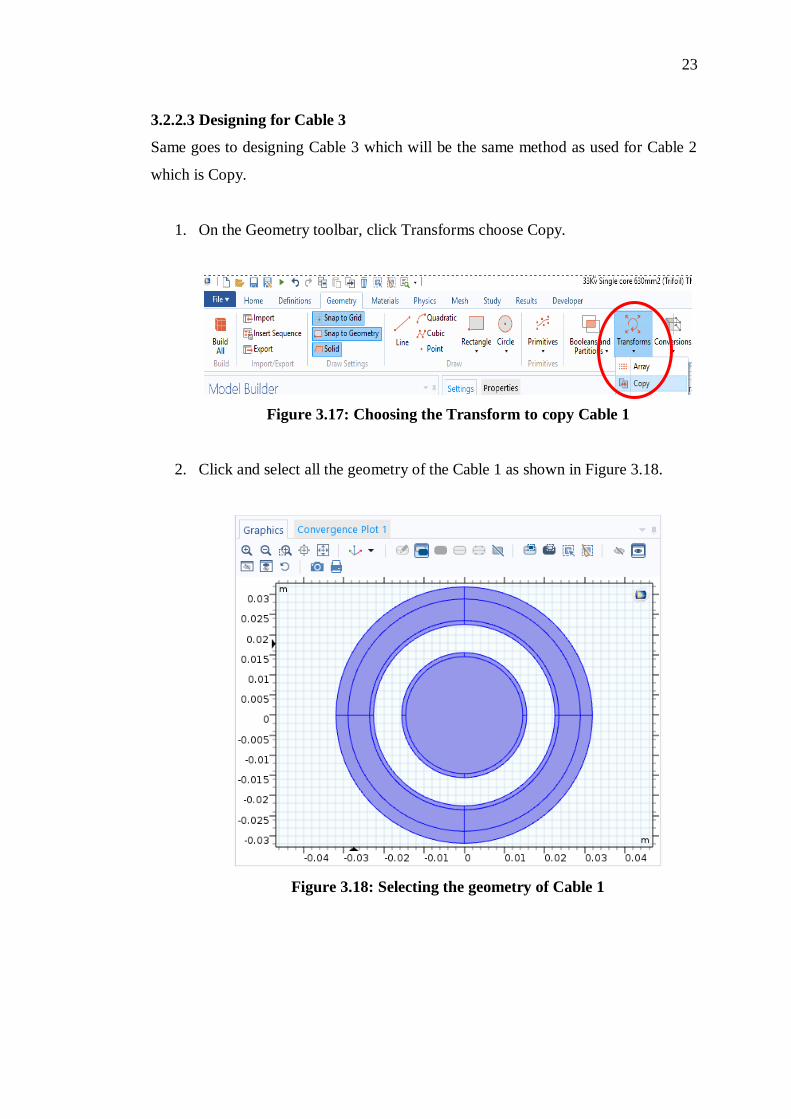
3.2.2.3 Designing for Cable 3
Same goes to designing Cable 3 which will be the same method as used for Cable 2
which is Copy.
1. On the Geometry toolbar, click Transforms choose Copy.
Figure 3.17: Choosing the Transform to copy Cable 1
2. Click and select all the geometry of the Cable 1 as shown in Figure 3.18.
Figure 3.18: Selecting the geometry of Cable 1
24
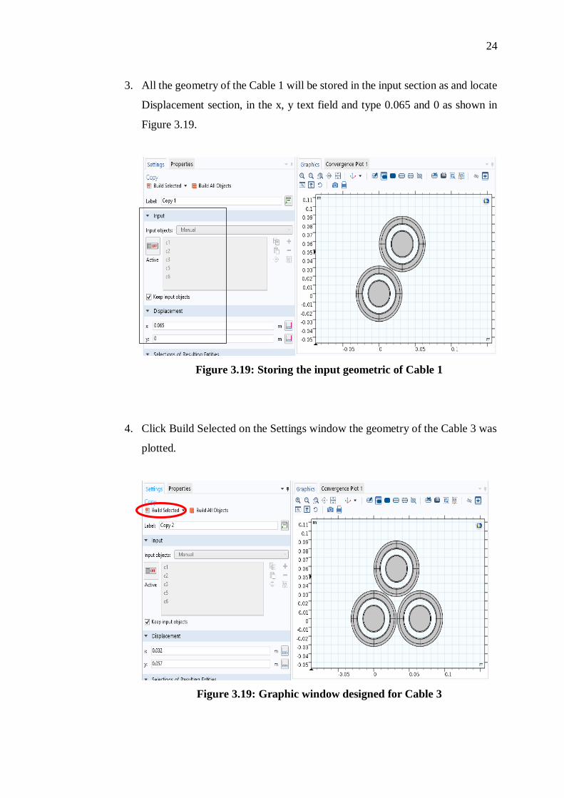
3. All the geometry of the Cable 1 will be stored in the input section as and locate
Displacement section, in the x, y text field and type 0.065 and 0 as shown in
Figure 3.19.
Figure 3.19: Storing the input geometric of Cable 1
4. Click Build Selected on the Settings window the geometry of the Cable 3 was
plotted.
Figure 3.19: Graphic window designed for Cable 3
25
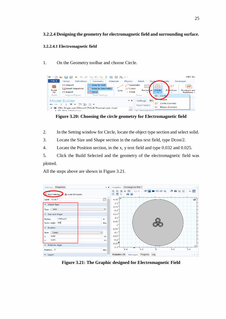
3.2.2.4 Designing the geometry for electromagnetic field and surrounding surface.
3.2.2.4.1 Electromagnetic field
1. On the Geometry toolbar and choose Circle.
Figure 3.20: Choosing the circle geometry for Electromagnetic field
2. In the Setting window for Circle, locate the object type section and select solid.
3. Locate the Size and Shape section in the radius text field, type Dcon/2.
4. Locate the Position section, in the x, y text field and type 0.032 and 0.025.
5. Click the Build Selected and the geometry of the electromagnetic field was
plotted.
All the steps above are shown in Figure 3.21.
Figure 3.21: The Graphic designed for Electromagnetic Field

26
3.2.2.4.2 Surrounding Surface
1. On the Geometry toolbar and choose Rectangular.
Figure 3.22: Choosing the circle geometry for Surrounding Surface
2. In the Setting window for Rectangle, locate the object type section and select
solid.
3. Locate the Size and Shape section, under the width and height type 10[m] and
8[m].
4. Locate the Position section, in the x, y text field and type -5[m] and -4[m].
5. Locate the Layer section, under Layer 1 type 5[m] for the boundary between
two section.
6. Click the Build Selected and the geometry of the surrounding surface was
plotted.
All the steps above are shown in Figure 3.23.
Figure 3.23: The graphic window designed of surrounding surface
27
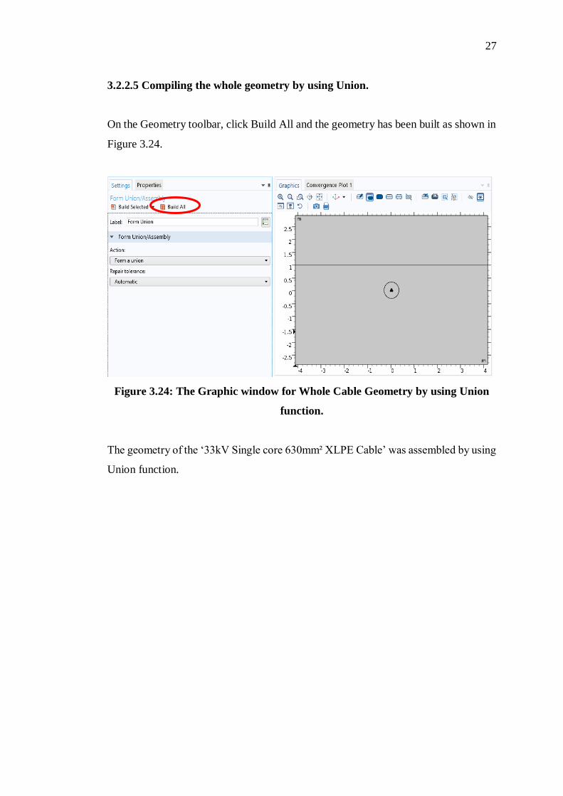
3.2.2.5 Compiling the whole geometry by using Union.
On the Geometry toolbar, click Build All and the geometry has been built as shown in
Figure 3.24.
Figure 3.24: The Graphic window for Whole Cable Geometry by using Union
function.
The geometry of the ‘33kV Single core 630mm² XLPE Cable’ was assembled by using
Union function.

28
3.2.3 Defining the Geometry of the Underground Power Cable (UPC)
Next, defining all geometry by characterization for every layer of the cable.
3.2.3.1 Defining for the Cables
1. On the Definitions toolbar, click Explicit.
Figure 3.25: Choosing the Explicit for Cables.
2. Type Cable in the Label text field under the Settings window for Explicit.
3. Click on the cables geometry to highlight the cable and the geometry entities
are stored in Input Entities.
4. The definition for the Cables is completed.
All the steps above are shown in Figure 3.26.
Figure 3.26: The Graphic window for the Definition of the Cables
29
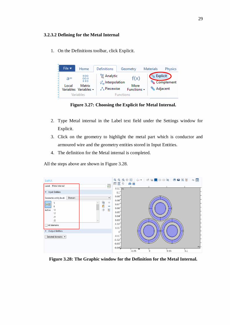
3.2.3.2 Defining for the Metal Internal
1. On the Definitions toolbar, click Explicit.
Figure 3.27: Choosing the Explicit for Metal Internal.
2. Type Metal internal in the Label text field under the Settings window for
Explicit.
3. Click on the geometry to highlight the metal part which is conductor and
armoured wire and the geometry entities stored in Input Entities.
4. The definition for the Metal internal is completed.
All the steps above are shown in Figure 3.28.
Figure 3.28: The Graphic window for the Definition for the Metal Internal.
30
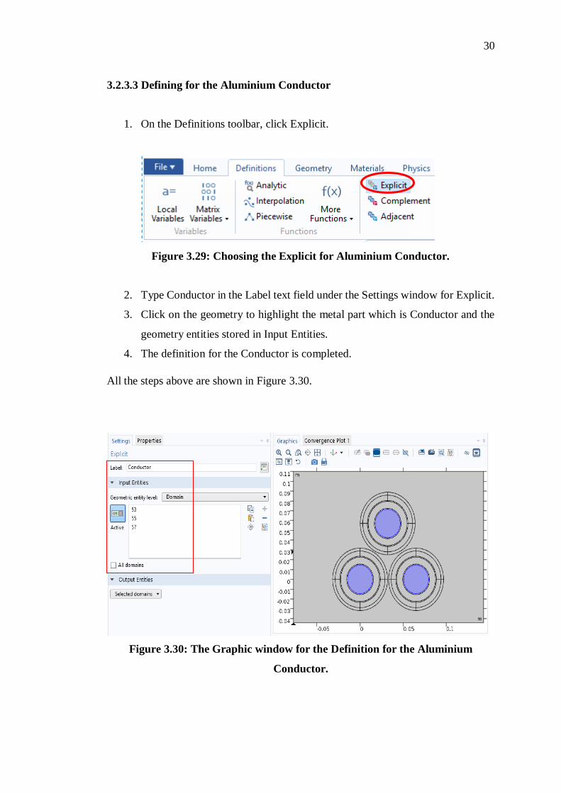
3.2.3.3 Defining for the Aluminium Conductor
1. On the Definitions toolbar, click Explicit.
Figure 3.29: Choosing the Explicit for Aluminium Conductor.
2. Type Conductor in the Label text field under the Settings window for Explicit.
3. Click on the geometry to highlight the metal part which is Conductor and the
geometry entities stored in Input Entities.
4. The definition for the Conductor is completed.
All the steps above are shown in Figure 3.30.
Figure 3.30: The Graphic window for the Definition for the Aluminium
Conductor.

31
3.2.3.4 Defining for the Insulation Internal (XLPE)
1. On the Definitions toolbar, click Explicit.
Figure 3.31: Choosing the Explicit for Insulation internal (XLPE).
2. Type Insulation internal in the Label text field under the Settings window for
Explicit.
3. Click on the geometry to highlight the insulation layer which is insulation
(XLPE) and the geometry entities stored in Input Entities.
4. The definition for the Insulation internal is completed.
All the steps above are shown in Figure 3.32.
Figure 3.32: The Graphic window for the Definition for the Insulation Internal.

32
3.2.3.5 Defining for the Semi-conductive compound
1. On the Definitions toolbar, click Explicit.
Figure 3.33: Choosing the Explicit for Semi-conductive compound.
2. Type Semiconductor in the Label text field under the Settings window for
Explicit.
3. Click on the geometry to highlight the semi conductive layer which is Semi-
conductor and the geometry entities stored in Input Entities.
4. The definition for the Semiconductor is completed.
All the steps above are shown in Figure 3.34.
Figure 3.34: The Graphic window for the Definition for the Semi-conductive
compound.
33
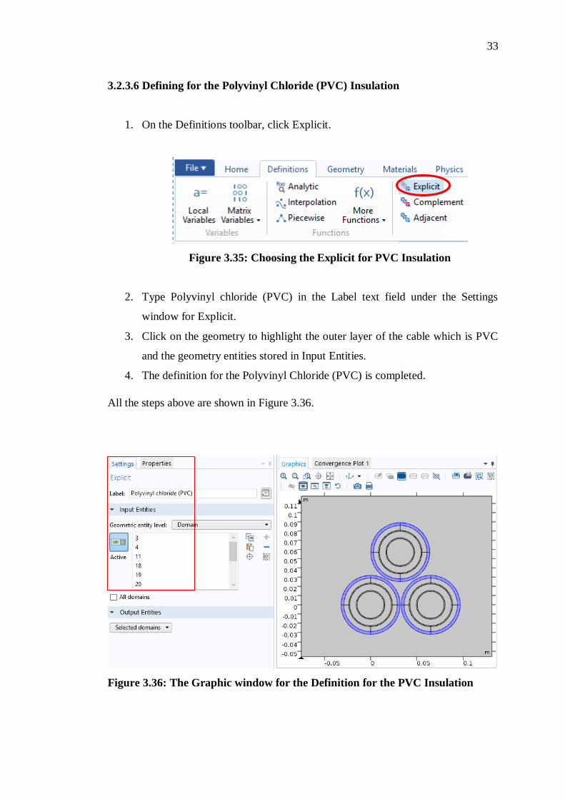
3.2.3.6 Defining for the Polyvinyl Chloride (PVC) Insulation
1. On the Definitions toolbar, click Explicit.
Figure 3.35: Choosing the Explicit for PVC Insulation
2. Type Polyvinyl chloride (PVC) in the Label text field under the Settings
window for Explicit.
3. Click on the geometry to highlight the outer layer of the cable which is PVC
and the geometry entities stored in Input Entities.
4. The definition for the Polyvinyl Chloride (PVC) is completed.
All the steps above are shown in Figure 3.36.
Figure 3.36: The Graphic window for the Definition for the PVC Insulation

34
3.2.3.7 Defining for the Armoured Wires
1. On the Definitions toolbar, click Explicit.
Figure 3.37: Choosing the Explicit function for Armoured Wires
2. Type Armoured Wires in the Label text field under the Settings window for
Explicit.
3. Click on the geometry to highlight the metal part of the cable which is
Armoured Wire and the geometry entities stored in Input Entities.
4. The definition for the Armoured Wire is completed.
All the steps above are shown in Figure 3.38.
Figure 3.38: The Graphic window for the Definition for the Armoured Wires
35
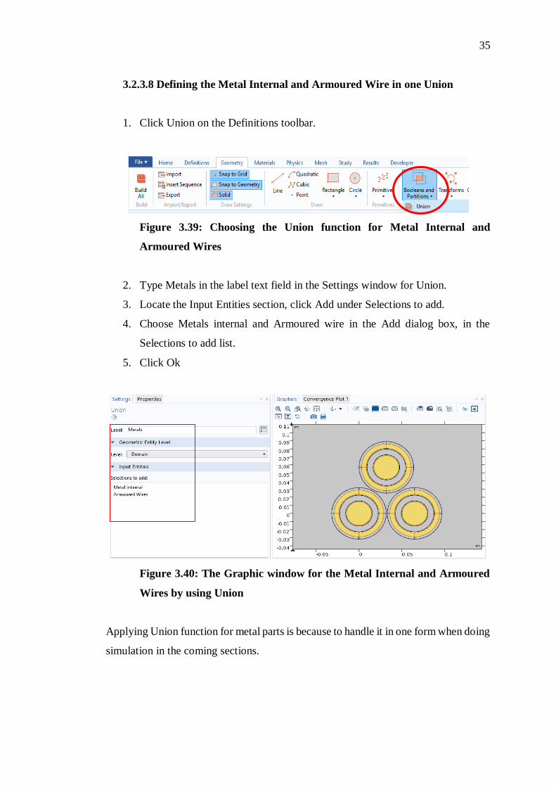
3.2.3.8 Defining the Metal Internal and Armoured Wire in one Union
1. Click Union on the Definitions toolbar.
Figure 3.39: Choosing the Union function for Metal Internal and
Armoured Wires
2. Type Metals in the label text field in the Settings window for Union.
3. Locate the Input Entities section, click Add under Selections to add.
4. Choose Metals internal and Armoured wire in the Add dialog box, in the
Selections to add list.
5. Click Ok
Figure 3.40: The Graphic window for the Metal Internal and Armoured
Wires by using Union
Applying Union function for metal parts is because to handle it in one form when doing
simulation in the coming sections.

36
3.2.4 Selecting the Material Type for the Underground Power Cable (UPC)
After completing defining the geometry of the cable, the next steps will be adding the
material type to the cables. The material properties that was used for 33kV Single core
630mm² XLPE Cable are shown in Table 1. In addition, the parameters for thermal
conductivity, density, for the following materials was used from the COMSOL where
the values are all built-in the material section (Littmarck, 2015).
Material Thermal
conductivity, k
(W/mK)
Density, Rho (kg/m³) Heat Capacity,
Cp (J/kg.K)
Air k(T[1/K]) rho(pA[1/Pa], T[1/K]) Cp(T[1/K])
Soil 1 2020 2512
Water, liquid k(T[1/K]) rho(T[1/K]) Cp(T[1/K])
Polyvinyl
Chloride (PVC)
0.19 1760 1170
Cross-linked
polyethylene
(XLPE)
0.46 930 2302
Semi-
conductive
compound
10 1055 2405
Aluminium Ntcon*238 2700 900
Copper 400 7850 475
Table 3.1: The Materials properties of the ‘33kV Single core 630mm² XLPE
Cable”
37
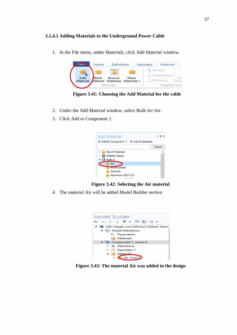
3.2.4.1 Adding Materials to the Underground Power Cable
1. In the File menu, under Materials, click Add Material window.
Figure 3.41: Choosing the Add Material for the cable
2. Under the Add Material window, select Built-In>Air.
3. Click Add to Component 1.
Figure 3.42: Selecting the Air material
4. The material Air will be added Model Builder section
Figure 3.43: The material Air was added in the design
38
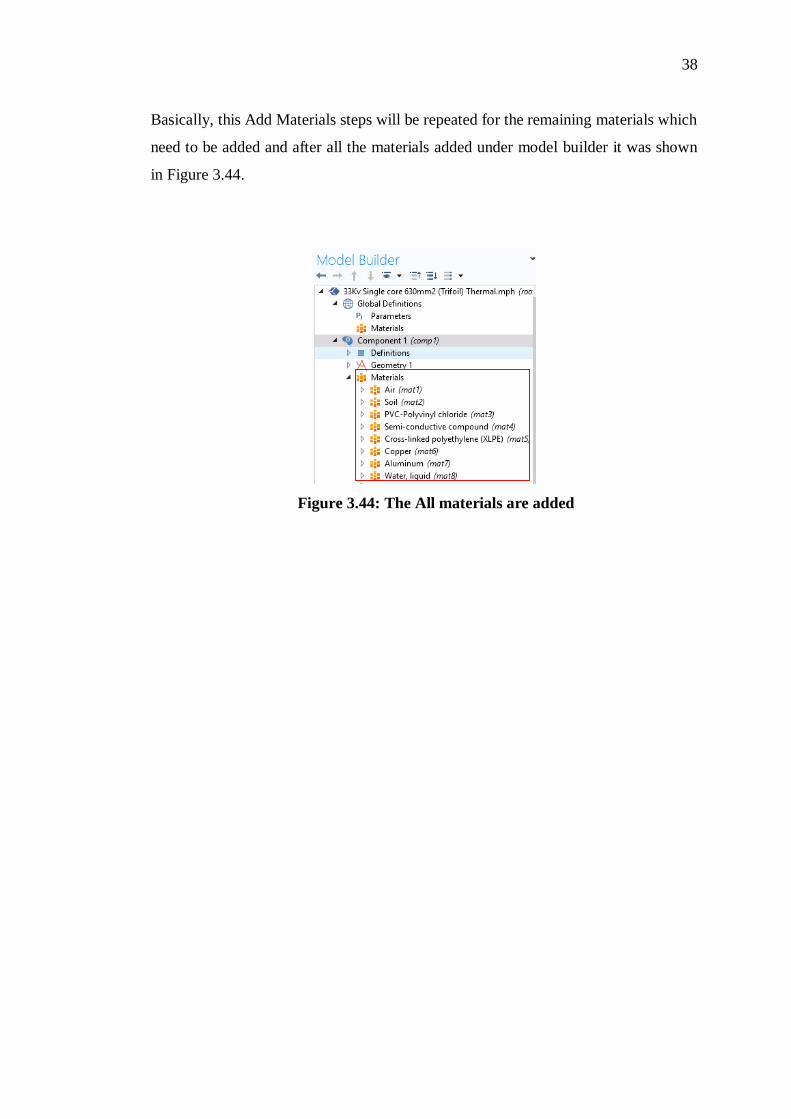
Basically, this Add Materials steps will be repeated for the remaining materials which
need to be added and after all the materials added under model builder it was shown
in Figure 3.44.
Figure 3.44: The All materials are added
39
3.2.4.2 Assigned materials for the Underground Power Cable
The final part for the material section is assigning the correct selection of the cable
structure using correct material.
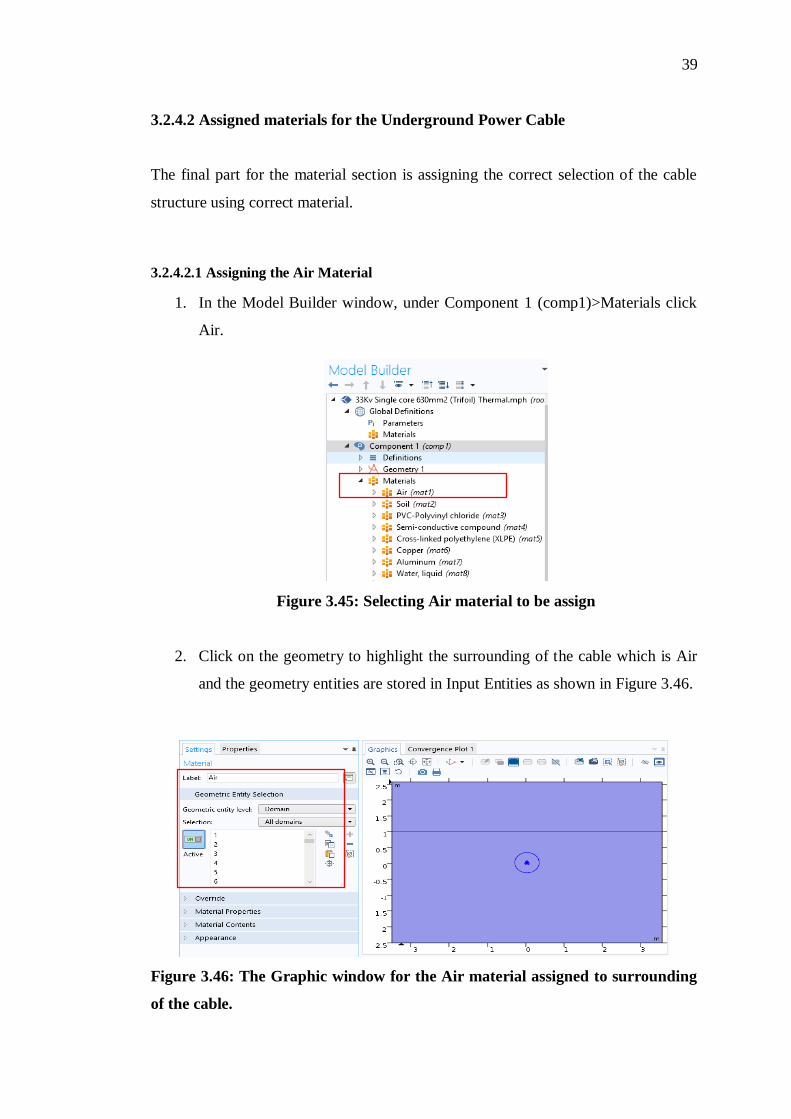
3.2.4.2.1 Assigning the Air Material
1. In the Model Builder window, under Component 1 (comp1)>Materials click
Air.
Figure 3.45: Selecting Air material to be assign
2. Click on the geometry to highlight the surrounding of the cable which is Air
and the geometry entities are stored in Input Entities as shown in Figure 3.46.
Figure 3.46: The Graphic window for the Air material assigned to surrounding
of the cable.
40
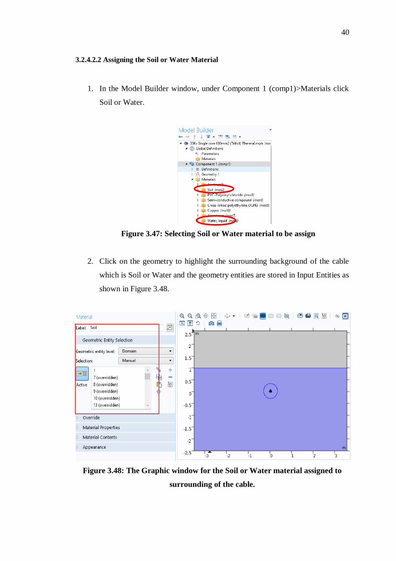
3.2.4.2.2 Assigning the Soil or Water Material
1. In the Model Builder window, under Component 1 (comp1)>Materials click
Soil or Water.
Figure 3.47: Selecting Soil or Water material to be assign
2. Click on the geometry to highlight the surrounding background of the cable
which is Soil or Water and the geometry entities are stored in Input Entities as
shown in Figure 3.48.
Figure 3.48: The Graphic window for the Soil or Water material assigned to
surrounding of the cable.

41
3.2.4.2.3 Assigning the Polyvinyl Chloride (PVC) Material
1. In the Model Builder window, under Component 1 (comp1)>Materials click
PVC.
Figure 3.49: Selecting Polyvinyl Chloride (PVC) material to be assign
2. Click on the geometry to highlight the outer layer of the cable which is PVC
and the geometry entities are stored in Input Entities as shown in Figure 3.50.
Figure 3.50: The Graphic window for Polyvinyl Chloride (PVC) assigned to the
cable.
42
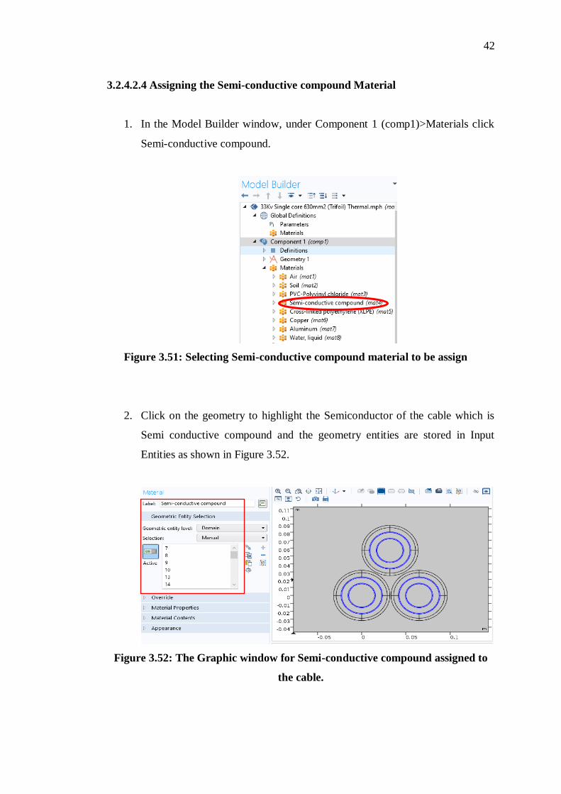
3.2.4.2.4 Assigning the Semi-conductive compound Material
1. In the Model Builder window, under Component 1 (comp1)>Materials click
Semi-conductive compound.
Figure 3.51: Selecting Semi-conductive compound material to be assign
2. Click on the geometry to highlight the Semiconductor of the cable which is
Semi conductive compound and the geometry entities are stored in Input
Entities as shown in Figure 3.52.
Figure 3.52: The Graphic window for Semi-conductive compound assigned to
the cable.
43
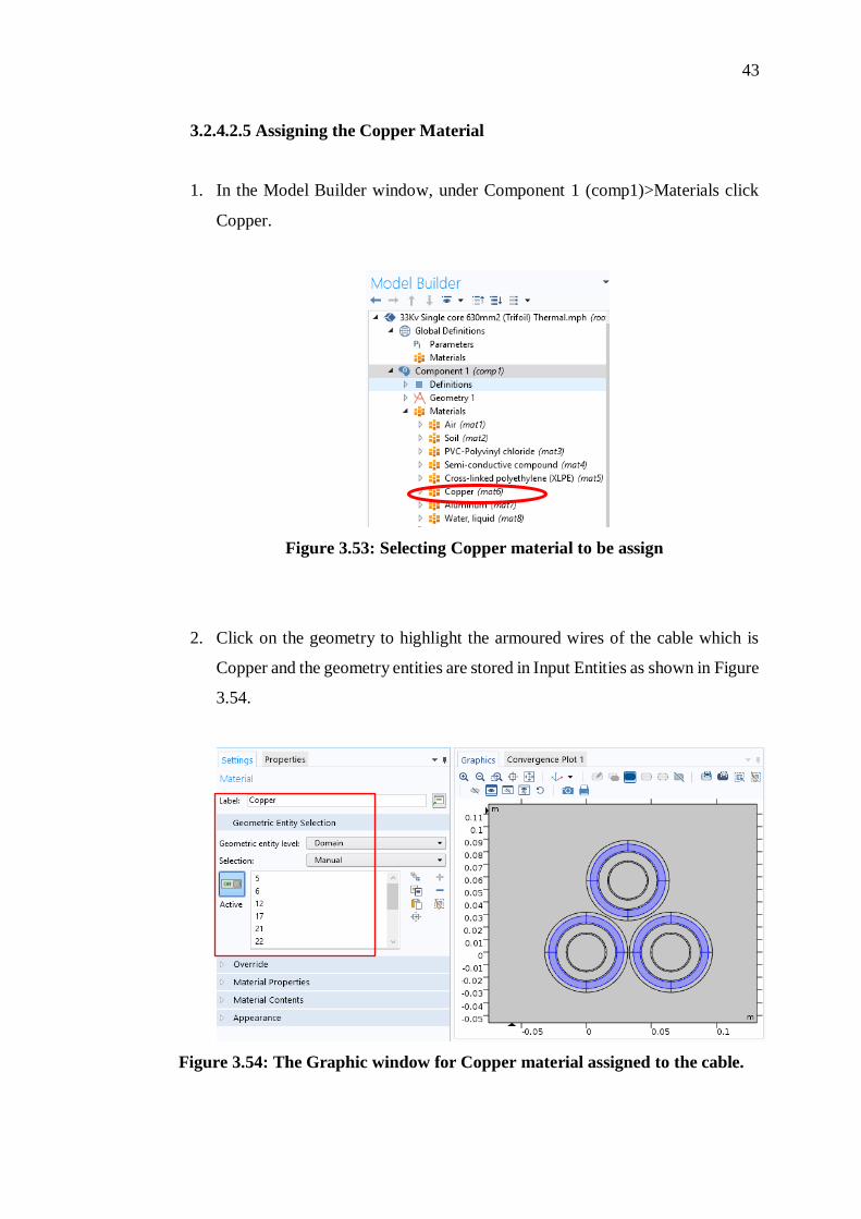
3.2.4.2.5 Assigning the Copper Material
1. In the Model Builder window, under Component 1 (comp1)>Materials click
Copper.
Figure 3.53: Selecting Copper material to be assign
2. Click on the geometry to highlight the armoured wires of the cable which is
Copper and the geometry entities are stored in Input Entities as shown in Figure
3.54.
Figure 3.54: The Graphic window for Copper material assigned to the cable.
44
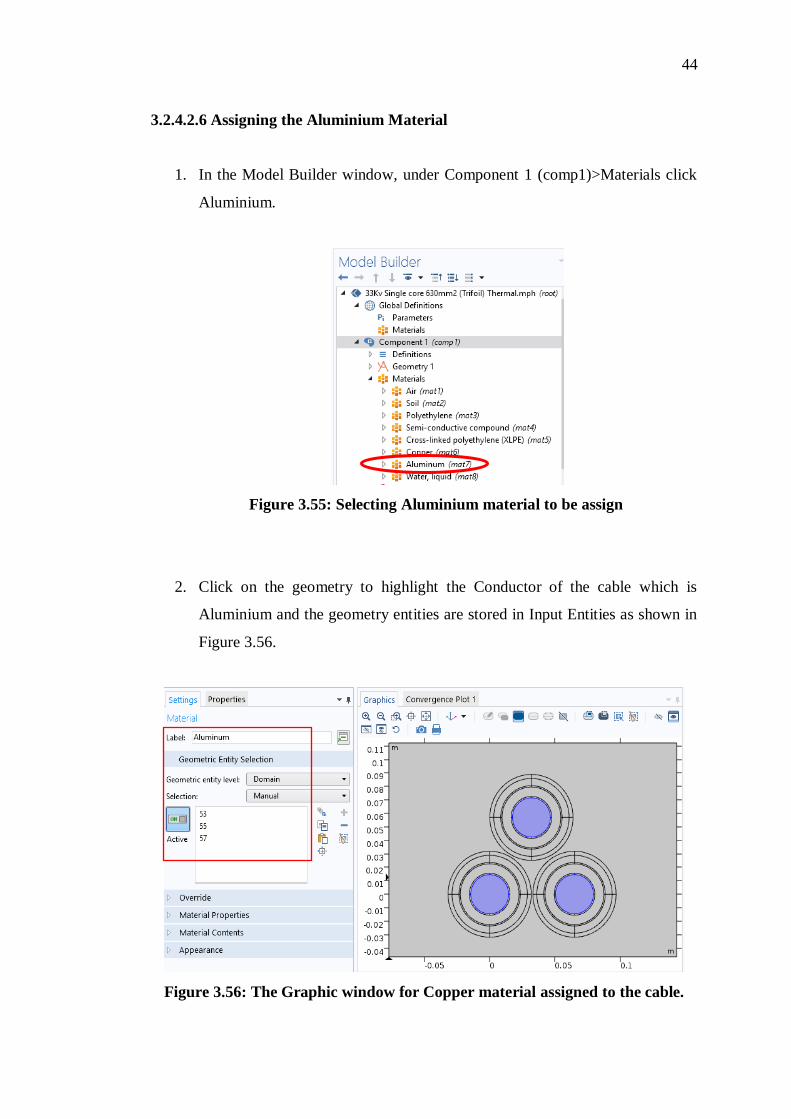
3.2.4.2.6 Assigning the Aluminium Material
1. In the Model Builder window, under Component 1 (comp1)>Materials click
Aluminium.
Figure 3.55: Selecting Aluminium material to be assign
2. Click on the geometry to highlight the Conductor of the cable which is
Aluminium and the geometry entities are stored in Input Entities as shown in
Figure 3.56.
Figure 3.56: The Graphic window for Copper material assigned to the cable.
45
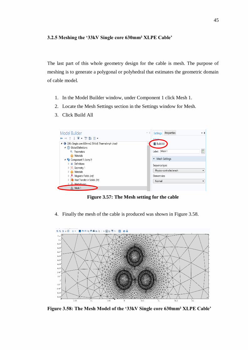
3.2.5 Meshing the ‘33kV Single core 630mm² XLPE Cable’
The last part of this whole geometry design for the cable is mesh. The purpose of
meshing is to generate a polygonal or polyhedral that estimates the geometric domain
of cable model.
1. In the Model Builder window, under Component 1 click Mesh 1.
2. Locate the Mesh Settings section in the Settings window for Mesh.
3. Click Build All
Figure 3.57: The Mesh setting for the cable
4. Finally the mesh of the cable is produced was shown in Figure 3.58.
Figure 3.58: The Mesh Model of the ‘33kV Single core 630mm² XLPE Cable’
46
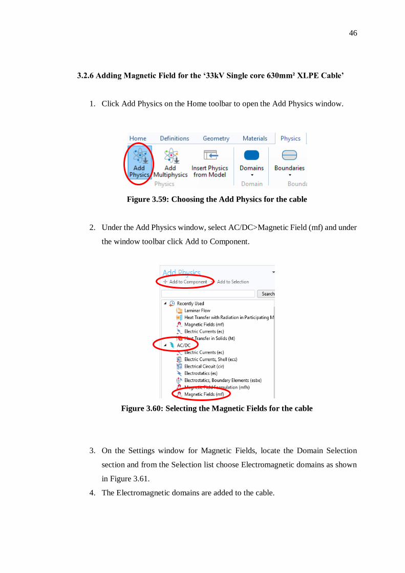
3.2.6 Adding Magnetic Field for the ‘33kV Single core 630mm² XLPE Cable’
1. Click Add Physics on the Home toolbar to open the Add Physics window.
Figure 3.59: Choosing the Add Physics for the cable
2. Under the Add Physics window, select AC/DC>Magnetic Field (mf) and under
the window toolbar click Add to Component.
Figure 3.60: Selecting the Magnetic Fields for the cable
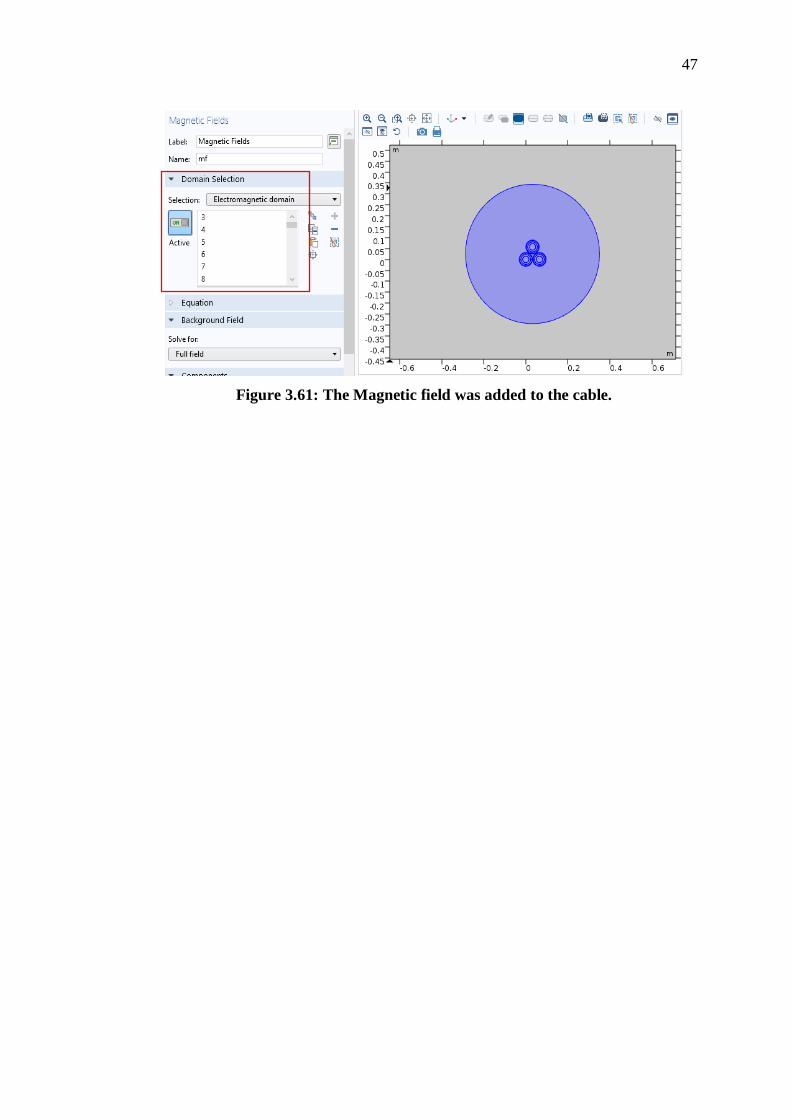
3. On the Settings window for Magnetic Fields, locate the Domain Selection
section and from the Selection list choose Electromagnetic domains as shown
in Figure 3.61.
4. The Electromagnetic domains are added to the cable.
47
Figure 3.61: The Magnetic field was added to the cable.

48
3.2.7 Adding the Thermal effect to the ‘33kV Single core 630mm² XLPE Cable’
1. Click Add Physics on the Home toolbar to open the Add Physics window.
Figure 3.62: Choosing the Add Physics for the cable
2. Under the Add Physics window, select Heat Transfer>Heat Transfer in Solids
(ht) and under the window toolbar click Add to Component.
Figure 3.63: Selecting the Heat Transfer in Solids for the cable
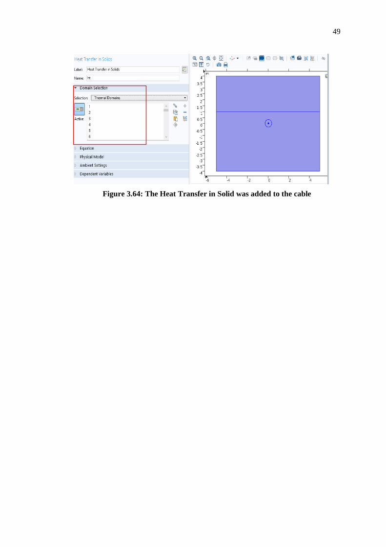
3. On the Settings window for Heat Transfer in Solids, locate the Domain
Selection section and from the Selection list choose Thermal domains as shown
in Figure 3.64.
4. The Thermal domains are added to the cable.
49
Figure 3.64: The Heat Transfer in Solid was added to the cable
50
3.2.8 Adding the Multiphysics Couplings to the ‘33kV Single core 630mm² XLPE
Cable’
The next step is to use Multiphysics Couplings which is coupling method where it
combines the Magnetic Flux and Heat Transfer in solid to form the Electromagnetic
Heating. This method was used so that electromagnetic losses results in generation of
heat. Therefore, it creates temperature dependent properties in the Magnetic Field
boundary which are related to the temperature values determined by Heat Transfer in
Solids (Kalenderli).
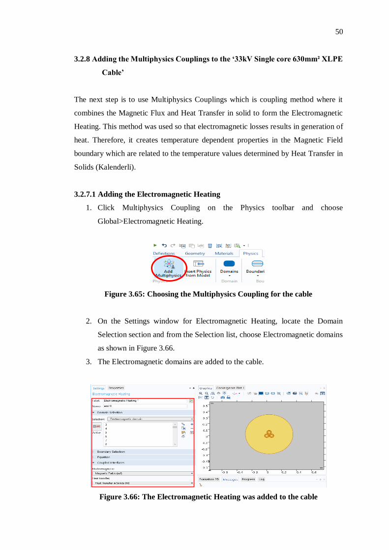
3.2.7.1 Adding the Electromagnetic Heating
1. Click Multiphysics Coupling on the Physics toolbar and choose
Global>Electromagnetic Heating.
Figure 3.65: Choosing the Multiphysics Coupling for the cable
2. On the Settings window for Electromagnetic Heating, locate the Domain
Selection section and from the Selection list, choose Electromagnetic domains
as shown in Figure 3.66.
3. The Electromagnetic domains are added to the cable.
Figure 3.66: The Electromagnetic Heating was added to the cable
51
3.2.7.2 Adding the Temperature
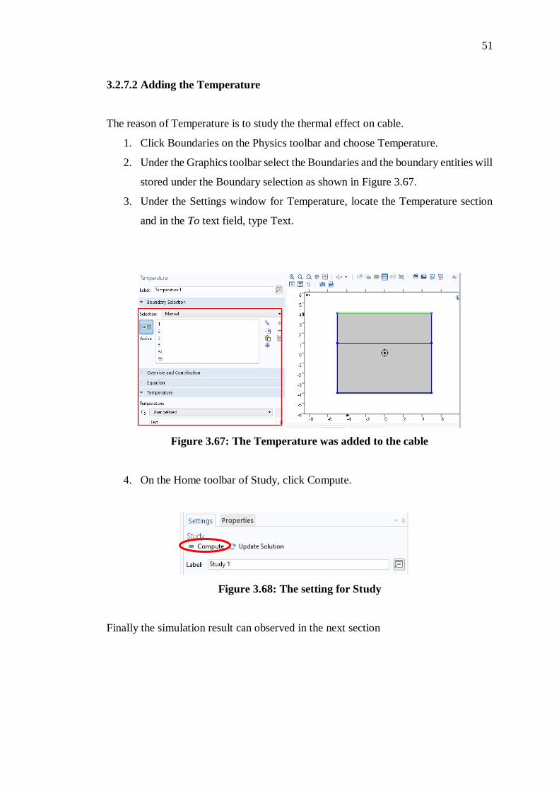
The reason of Temperature is to study the thermal effect on cable.
1. Click Boundaries on the Physics toolbar and choose Temperature.
2. Under the Graphics toolbar select the Boundaries and the boundary entities will
stored under the Boundary selection as shown in Figure 3.67.
3. Under the Settings window for Temperature, locate the Temperature section
and in the To text field, type Text.
Figure 3.67: The Temperature was added to the cable
4. On the Home toolbar of Study, click Compute.
Figure 3.68: The setting for Study
Finally the simulation result can observed in the next section
52
3.2.7.3 The Result of the Temperature (ht)
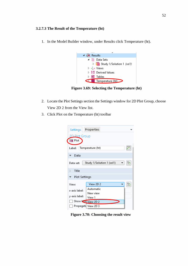
1. In the Model Builder window, under Results click Temperature (ht).
Figure 3.69: Selecting the Temperature (ht)
2. Locate the Plot Settings section the Settings window for 2D Plot Group, choose
View 2D 2 from the View list.
3. Click Plot on the Temperature (ht) toolbar
Figure 3.70: Choosing the result view

53
4. The design of the heat transfer on the cable will be displayed shown in Figure
3.71.
Figure 3.71: The heat transfer on the cable
54
3.2.8 Complete design of 33kV Single Core 630mm² Al XLPE Cable by using
COMSOL software.
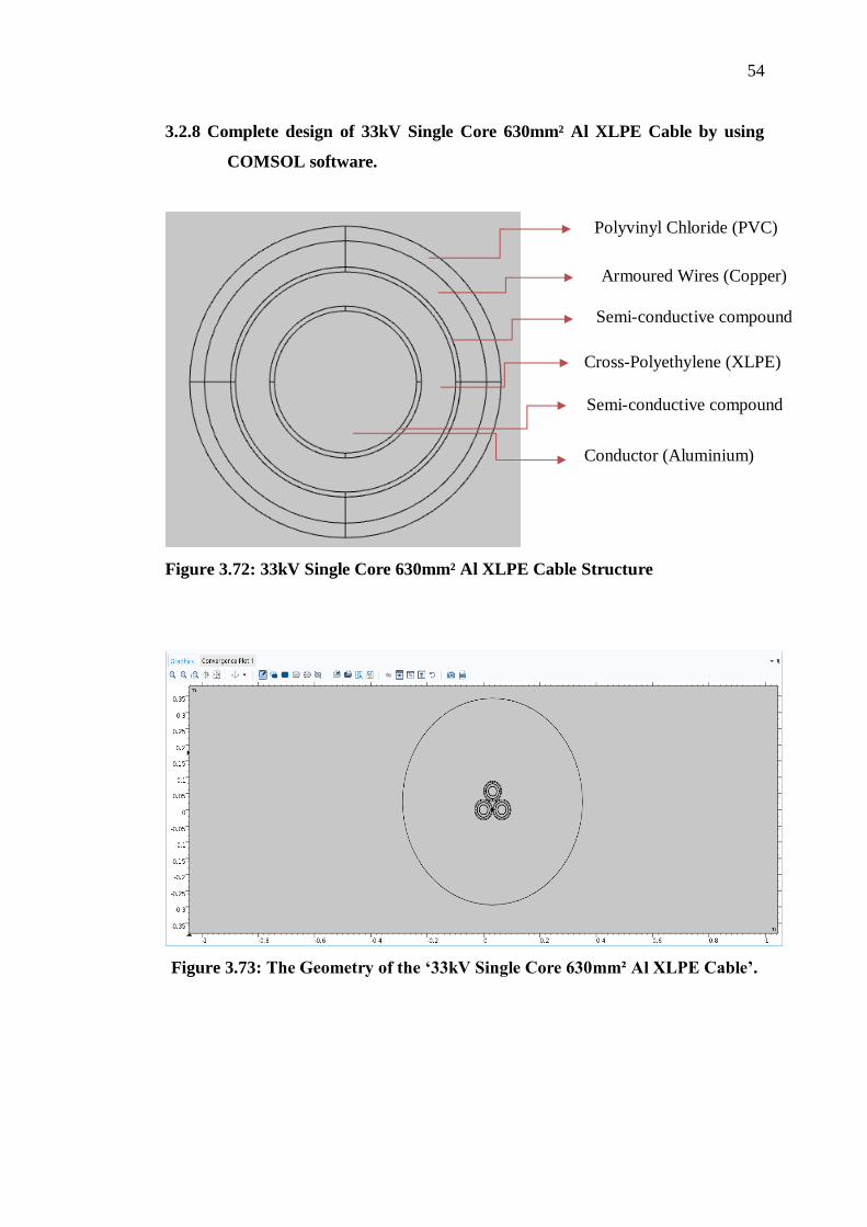
Figure 3.72: 33kV Single Core 630mm² Al XLPE Cable Structure
Figure 3.73: The Geometry of the ‘33kV Single Core 630mm² Al XLPE Cable’.
Polyvinyl Chloride (PVC)
Armoured Wires (Copper)
Semi-conductive compound
Semi-conductive compound
Cross-Polyethylene (XLPE)
Conductor (Aluminium)
55
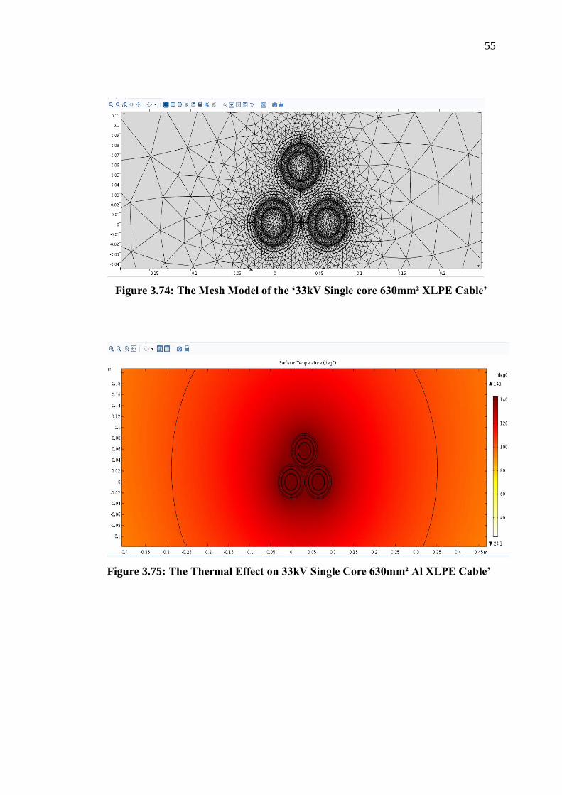
Figure 3.74: The Mesh Model of the ‘33kV Single core 630mm² XLPE Cable’
Figure 3.75: The Thermal Effect on 33kV Single Core 630mm² Al XLPE Cable’
56
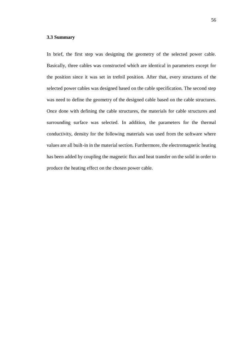
3.3 Summary
In brief, the first step was designing the geometry of the selected power cable.
Basically, three cables was constructed which are identical in parameters except for
the position since it was set in trefoil position. After that, every structures of the
selected power cables was designed based on the cable specification. The second step
was need to define the geometry of the designed cable based on the cable structures.
Once done with defining the cable structures, the materials for cable structures and
surrounding surface was selected. In addition, the parameters for the thermal
conductivity, density for the following materials was used from the software where
values are all built-in in the material section. Furthermore, the electromagnetic heating
has been added by coupling the magnetic flux and heat transfer on the solid in order to
produce the heating effect on the chosen power cable.

57
CHAPTER 4
1 RESULT AND DISCUSSSION
4.1 Introduction
In this chapter, it shows that the thermal analysis has been conducted on the
‘33kV Single Core 630mm² Al XLPE Cable’. This simulation test was done in order
to obtain the operating temperature with different soil conditions with the current
correction factor (CF) and without the current correction factor (CF) by changing the
soil temperature, different cable positions, different cable depth buried into the ground
and also with water.
4.2 Thermal effect on single-core cable
In this work, the 33KV Single Core 1x630mm² XLPE Cable was used as mentioned
before. Therefore, this cable has been used to analyse the thermal effect under two
different depth burial of the cable under the soil which is 0.5 and 1 meter as shown in
Figure 4.2 and 4.5. The soil condition which was used for this analysis are dry type.
The ambient ground temperature was fixed at 35°C. In addition, the minimum current
value that was used in this simulation test are the operating current value of the power
cable from the data sheet which is 𝐼𝑎 = 685A and this value was increased to the
maximum current rating in order to obtain the maximum cables conductors operating
temperature (°C) which is 90°C of the underground power cables (UPC) selected for
this research.

58
4.2.1 The Single Cable Buried Cable Under 0.5 meter Depth
Figure 4.1: The single cable buried in depth of 0.5 meter.
Figure 4.2: The operating temperature on underground power cables (UPC)
buried in depth of 0.5 meter (Zoom in view).
0.5
meter
59
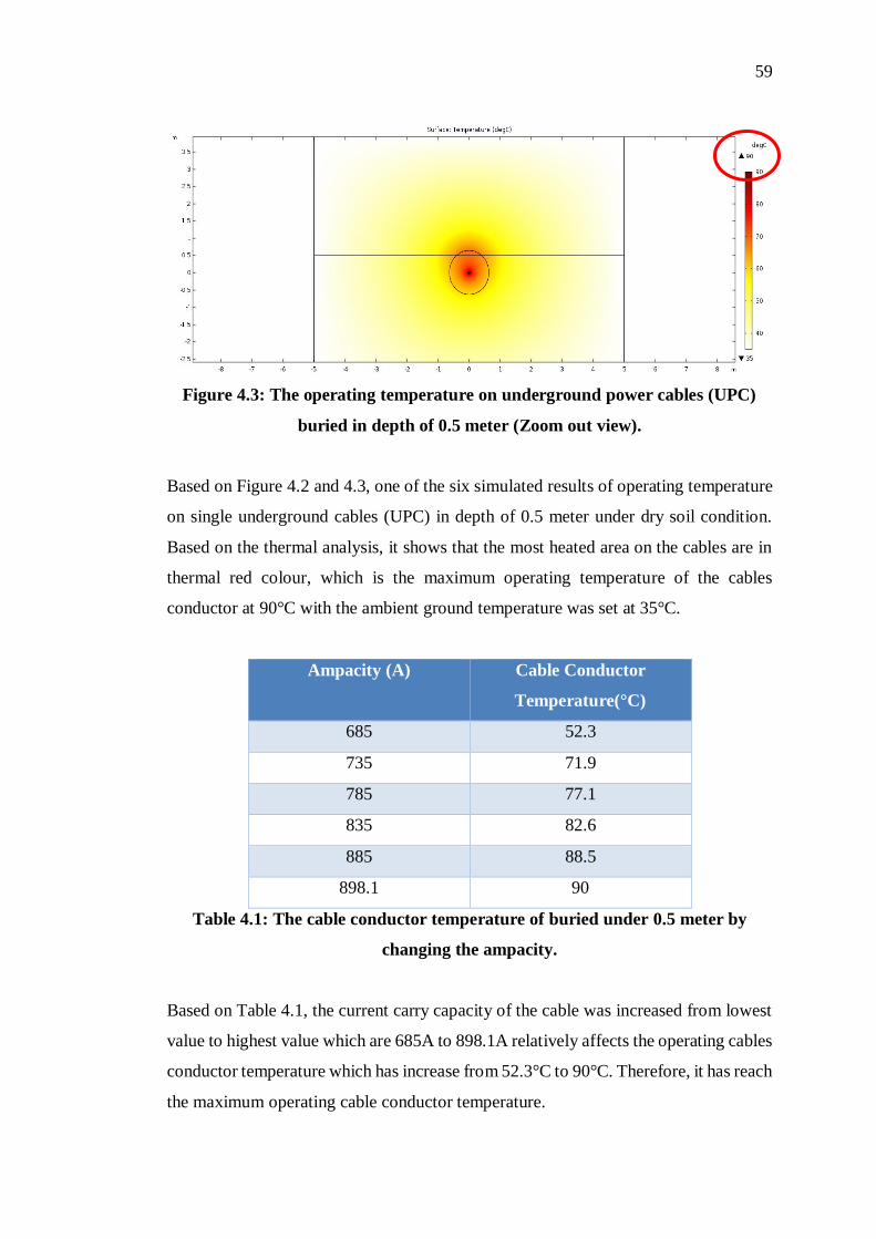
Figure 4.3: The operating temperature on underground power cables (UPC)
buried in depth of 0.5 meter (Zoom out view).
Based on Figure 4.2 and 4.3, one of the six simulated results of operating temperature
on single underground cables (UPC) in depth of 0.5 meter under dry soil condition.
Based on the thermal analysis, it shows that the most heated area on the cables are in
thermal red colour, which is the maximum operating temperature of the cables
conductor at 90°C with the ambient ground temperature was set at 35°C.
Ampacity (A)
Cable Conductor
Temperature(°C)
685 52.3
735 71.9
785 77.1
835 82.6
885 88.5
898.1 90
Table 4.1: The cable conductor temperature of buried under 0.5 meter by
changing the ampacity.
Based on Table 4.1, the current carry capacity of the cable was increased from lowest
value to highest value which are 685A to 898.1A relatively affects the operating cables
conductor temperature which has increase from 52.3°C to 90°C. Therefore, it has reach
the maximum operating cable conductor temperature.
60
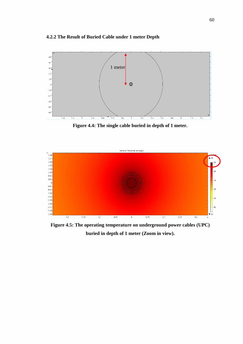
4.2.2 The Result of Buried Cable under 1 meter Depth
Figure 4.4: The single cable buried in depth of 1 meter.
Figure 4.5: The operating temperature on underground power cables (UPC)
buried in depth of 1 meter (Zoom in view).
1 meter
61
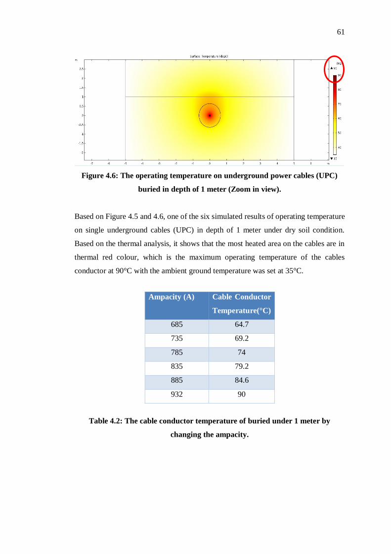
Figure 4.6: The operating temperature on underground power cables (UPC)
buried in depth of 1 meter (Zoom in view).
Based on Figure 4.5 and 4.6, one of the six simulated results of operating temperature
on single underground cables (UPC) in depth of 1 meter under dry soil condition.
Based on the thermal analysis, it shows that the most heated area on the cables are in
thermal red colour, which is the maximum operating temperature of the cables
conductor at 90°C with the ambient ground temperature was set at 35°C.
Table 4.2: The cable conductor temperature of buried under 1 meter by
changing the ampacity.
Ampacity (A)
Cable Conductor
Temperature(°C)
685 64.7
735 69.2
785 74
835 79.2
885 84.6
932 90

62
Based on Table 4.2, the current carry capacity of the cable was increased from the
lowest value to the highest value which are 685A to 932A correspondingly affects the
operating cables conductor temperature which has increase from 64.7°C to 90°C.
Therefore, it has reach the maximum operating cable conductor temperature.
4.2.3 Comparison of the result of the two cable depth of the buried in 0.5 meter
and 1 meter.
Ampacity (A)
for 0.5 meter
Cable Conductor
Temperature(°C)
for 0.5 meter
Ampacity (A)
for 1 meter
Cable Conductor
Temperature(°C)
for 1 meter
685 67.4 685 64.7
735 71.9 735 69.2
785 77.1 785 74
835 82.6 835 79.2
885 88.5 885 84.6
898.1 90 898.1 86.1
932 98.4 932 90
Table 4.3: The two cable depth of the buried in 0.5 meter and 1 meter.
Figure 4.7: The two cable depth of the buried in 0.5 meter and 1 meter.
0102030405060708090
100
685 735 785 835 885 898.1 932
The operating cable conductor temperature against ampacity.
Cable Conductor Temperature(°C) for 0.5 meter
Cable Conductor Temperature(°C) for 1 meter
AmpacityThe
op
erat
ing t
emp
erat
ure
of
cable
co
ndu
ctor
63
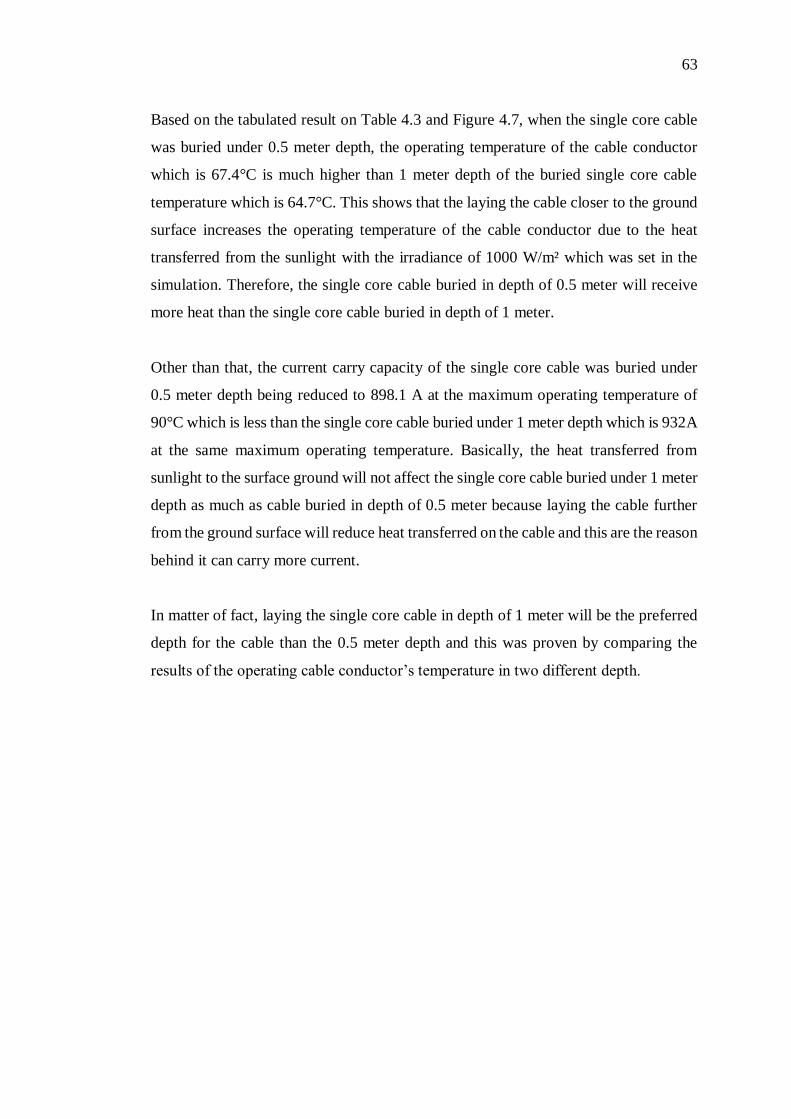
Based on the tabulated result on Table 4.3 and Figure 4.7, when the single core cable
was buried under 0.5 meter depth, the operating temperature of the cable conductor
which is 67.4°C is much higher than 1 meter depth of the buried single core cable
temperature which is 64.7°C. This shows that the laying the cable closer to the ground
surface increases the operating temperature of the cable conductor due to the heat
transferred from the sunlight with the irradiance of 1000 W/m² which was set in the
simulation. Therefore, the single core cable buried in depth of 0.5 meter will receive
more heat than the single core cable buried in depth of 1 meter.
Other than that, the current carry capacity of the single core cable was buried under
0.5 meter depth being reduced to 898.1 A at the maximum operating temperature of
90°C which is less than the single core cable buried under 1 meter depth which is 932A
at the same maximum operating temperature. Basically, the heat transferred from
sunlight to the surface ground will not affect the single core cable buried under 1 meter
depth as much as cable buried in depth of 0.5 meter because laying the cable further
from the ground surface will reduce heat transferred on the cable and this are the reason
behind it can carry more current.
In matter of fact, laying the single core cable in depth of 1 meter will be the preferred
depth for the cable than the 0.5 meter depth and this was proven by comparing the
results of the operating cable conductor’s temperature in two different depth.
64
4.3 Effect of thermal conductivity of different types of soil on underground power
cables with current rating correction factors.
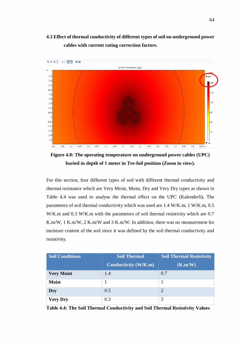
Figure 4.8: The operating temperature on underground power cables (UPC)
buried in depth of 1 meter in Tre-foil position (Zoom in view).
For this section, four different types of soil with different thermal conductivity and
thermal resistance which are Very Moist, Moist, Dry and Very Dry types as shown in
Table 4.4 was used to analyse the thermal effect on the UPC (Kalenderli). The
parameters of soil thermal conductivity which was used are 1.4 W/K.m, 1 W/K.m, 0.5
W/K.m and 0.3 W/K.m with the parameters of soil thermal resistivity which are 0.7
K.m/W, 1 K.m/W, 2 K.m/W and 3 K.m/W. In addition, there was no measurement for
moisture content of the soil since it was defined by the soil thermal conductivity and
resistivity.
Soil Conditions Soil Thermal
Conductivity (W/K.m)
Soil Thermal Resistivity
(K.m/W)
Very Moist 1.4 0.7
Moist 1 1
Dry 0.5 2
Very Dry 0.3 3
Table 4.4: The Soil Thermal Conductivity and Soil Thermal Resistivity Values
65
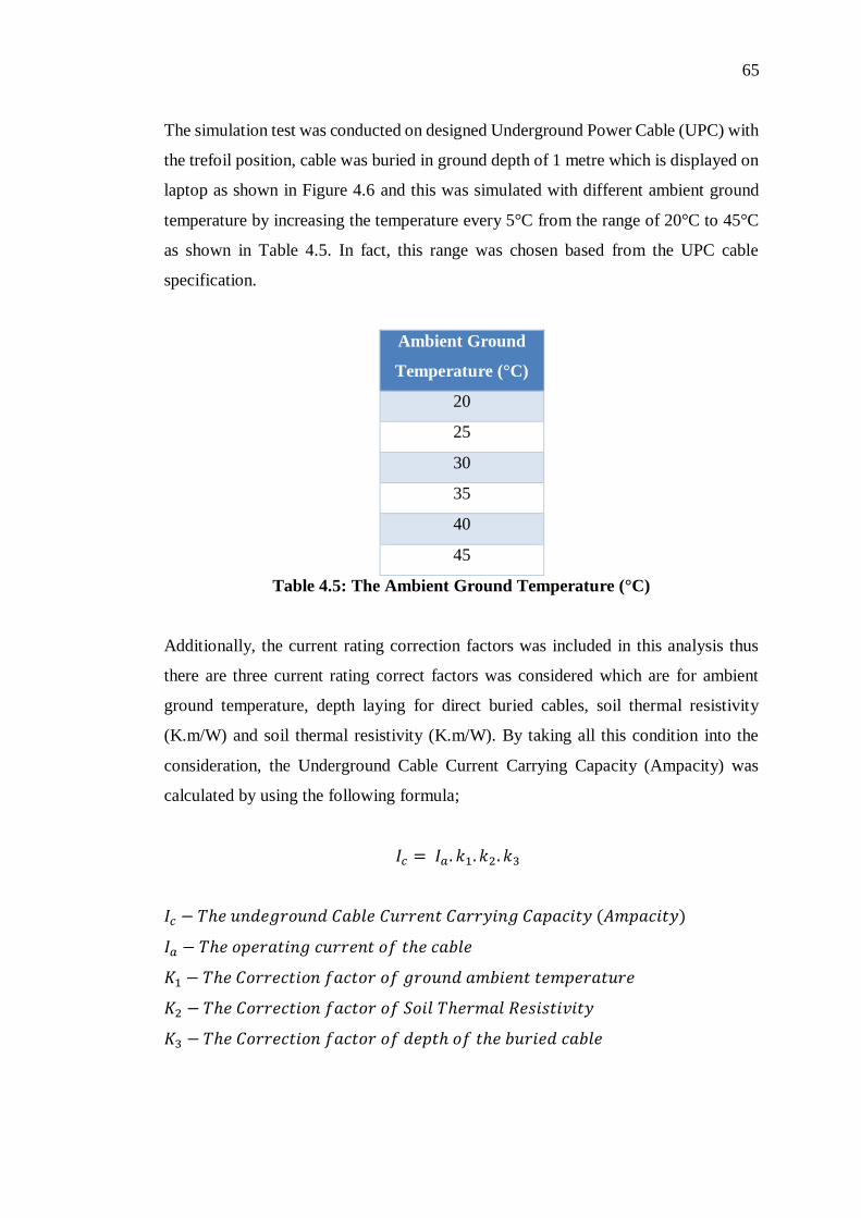
The simulation test was conducted on designed Underground Power Cable (UPC) with
the trefoil position, cable was buried in ground depth of 1 metre which is displayed on
laptop as shown in Figure 4.6 and this was simulated with different ambient ground
temperature by increasing the temperature every 5°C from the range of 20°C to 45°C
as shown in Table 4.5. In fact, this range was chosen based from the UPC cable
specification.
Ambient Ground
Temperature (°C)
20
25
30
35
40
45
Table 4.5: The Ambient Ground Temperature (°C)
Additionally, the current rating correction factors was included in this analysis thus
there are three current rating correct factors was considered which are for ambient
ground temperature, depth laying for direct buried cables, soil thermal resistivity
(K.m/W) and soil thermal resistivity (K.m/W). By taking all this condition into the
consideration, the Underground Cable Current Carrying Capacity (Ampacity) was
calculated by using the following formula;
𝐼𝑐 = 𝐼𝑎 . 𝑘1. 𝑘2. 𝑘3
𝐼𝑐 − 𝑇ℎ𝑒 𝑢𝑛𝑑𝑒𝑔𝑟𝑜𝑢𝑛𝑑 𝐶𝑎𝑏𝑙𝑒 𝐶𝑢𝑟𝑟𝑒𝑛𝑡 𝐶𝑎𝑟𝑟𝑦𝑖𝑛𝑔 𝐶𝑎𝑝𝑎𝑐𝑖𝑡𝑦 (𝐴𝑚𝑝𝑎𝑐𝑖𝑡𝑦)
𝐼𝑎 − 𝑇ℎ𝑒 𝑜𝑝𝑒𝑟𝑎𝑡𝑖𝑛𝑔 𝑐𝑢𝑟𝑟𝑒𝑛𝑡 𝑜𝑓 𝑡ℎ𝑒 𝑐𝑎𝑏𝑙𝑒
𝐾1 − 𝑇ℎ𝑒 𝐶𝑜𝑟𝑟𝑒𝑐𝑡𝑖𝑜𝑛 𝑓𝑎𝑐𝑡𝑜𝑟 𝑜𝑓 𝑔𝑟𝑜𝑢𝑛𝑑 𝑎𝑚𝑏𝑖𝑒𝑛𝑡 𝑡𝑒𝑚𝑝𝑒𝑟𝑎𝑡𝑢𝑟𝑒
𝐾2 − 𝑇ℎ𝑒 𝐶𝑜𝑟𝑟𝑒𝑐𝑡𝑖𝑜𝑛 𝑓𝑎𝑐𝑡𝑜𝑟 𝑜𝑓 𝑆𝑜𝑖𝑙 𝑇ℎ𝑒𝑟𝑚𝑎𝑙 𝑅𝑒𝑠𝑖𝑠𝑡𝑖𝑣𝑖𝑡𝑦
𝐾3 − 𝑇ℎ𝑒 𝐶𝑜𝑟𝑟𝑒𝑐𝑡𝑖𝑜𝑛 𝑓𝑎𝑐𝑡𝑜𝑟 𝑜𝑓 𝑑𝑒𝑝𝑡ℎ 𝑜𝑓 𝑡ℎ𝑒 𝑏𝑢𝑟𝑖𝑒𝑑 𝑐𝑎𝑏𝑙𝑒
66
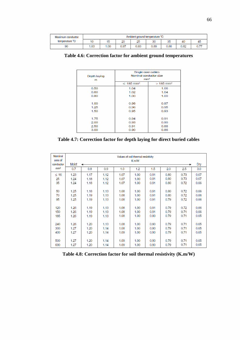
Table 4.6: Correction factor for ambient ground temperatures
Table 4.7: Correction factor for depth laying for direct buried cables
Table 4.8: Correction factor for soil thermal resistivity (K.m/W)
67
4.3.1 The Result of Operating Cable Conductor Temperature using Different Soil
Conditions with Correction Factor
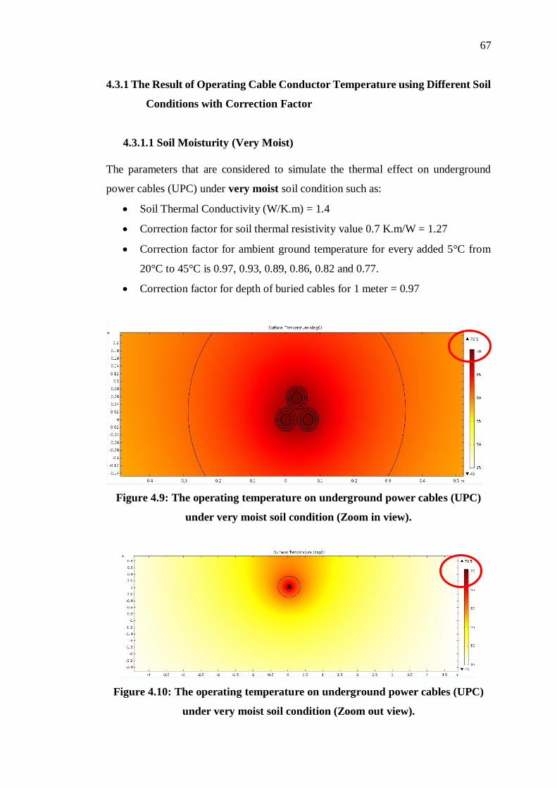
4.3.1.1 Soil Moisturity (Very Moist)
The parameters that are considered to simulate the thermal effect on underground
power cables (UPC) under very moist soil condition such as:
Soil Thermal Conductivity (W/K.m) = 1.4
Correction factor for soil thermal resistivity value 0.7 K.m/W = 1.27
Correction factor for ambient ground temperature for every added 5°C from
20°C to 45°C is 0.97, 0.93, 0.89, 0.86, 0.82 and 0.77.
Correction factor for depth of buried cables for 1 meter = 0.97
Figure 4.9: The operating temperature on underground power cables (UPC)
under very moist soil condition (Zoom in view).
Figure 4.10: The operating temperature on underground power cables (UPC)
under very moist soil condition (Zoom out view).

68
Based on Figure 4.9 and 4.10, one of the six simulated results of operating temperature
on underground cables (UPC) with current rating correction factor under very moist
soil condition. Based on the thermal analysis, it shows that the most heated area on the
cables are in thermal red colour, which is operating temperature of the cables
conductor at 70.5°C with the ambient ground temperature was set at 45°C.
Ambient Ground
Temperature (°C)
Ampacity (A) Cable Conductor
Temperature(°C)
20 818.5 60.5
25 784.78 62.2
30 751.03 64.1
35 725.71 66.8
40 691.96 68.9
45 649.77 70.5
Table 4.9: The Cable Conductor Temperature (°C) of Very Moist Soil
Condition
Based on Table 4.9, the ambient ground temperature was increased from 20°C to 45°C
and the ampacity for this temperature range decreases from the highest to lowest value
which are 818.5A to 649.77A. The operating cables conductor temperature has
increase from 60.5°C to 70.5°C respectively to the ambient ground temperature and
ampacity of the UPC.
69
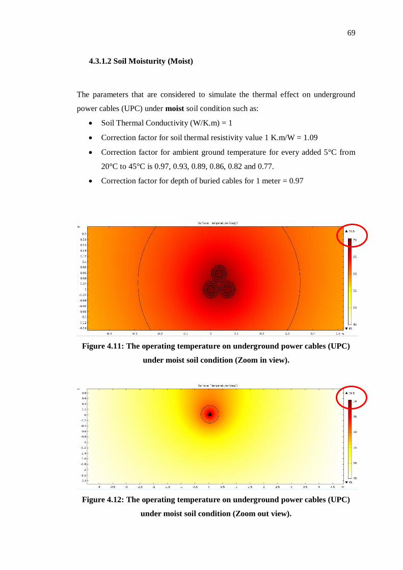
4.3.1.2 Soil Moisturity (Moist)
The parameters that are considered to simulate the thermal effect on underground
power cables (UPC) under moist soil condition such as:
Soil Thermal Conductivity (W/K.m) = 1
Correction factor for soil thermal resistivity value 1 K.m/W = 1.09
Correction factor for ambient ground temperature for every added 5°C from
20°C to 45°C is 0.97, 0.93, 0.89, 0.86, 0.82 and 0.77.
Correction factor for depth of buried cables for 1 meter = 0.97
Figure 4.11: The operating temperature on underground power cables (UPC)
under moist soil condition (Zoom in view).
Figure 4.12: The operating temperature on underground power cables (UPC)
under moist soil condition (Zoom out view).
70
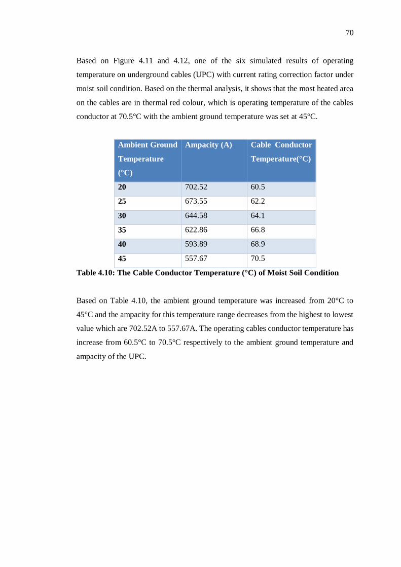
Based on Figure 4.11 and 4.12, one of the six simulated results of operating
temperature on underground cables (UPC) with current rating correction factor under
moist soil condition. Based on the thermal analysis, it shows that the most heated area
on the cables are in thermal red colour, which is operating temperature of the cables
conductor at 70.5°C with the ambient ground temperature was set at 45°C.
Ambient Ground
Temperature
(°C)
Ampacity (A) Cable Conductor
Temperature(°C)
20 702.52 60.5
25 673.55 62.2
30 644.58 64.1
35 622.86 66.8
40 593.89 68.9
45 557.67 70.5
Table 4.10: The Cable Conductor Temperature (°C) of Moist Soil Condition
Based on Table 4.10, the ambient ground temperature was increased from 20°C to
45°C and the ampacity for this temperature range decreases from the highest to lowest
value which are 702.52A to 557.67A. The operating cables conductor temperature has
increase from 60.5°C to 70.5°C respectively to the ambient ground temperature and
ampacity of the UPC.

71
4.3.1.3 Soil Moisturity (Dry)
The parameters that are considered to simulate the thermal effect on underground
power cables (UPC) under dry soil condition such as:
Soil Thermal Conductivity (W/K.m) = 0.5
Correction factor for soil thermal resistivity value 2 K.m/W = 0.79
Correction factor for ambient ground temperature for every added 5°C from
20°C to 45°C is 0.97, 0.93, 0.89, 0.86, 0.82 and 0.77.
Correction factor for depth of buried cables for 1 meter = 0.97
Figure 4.13: The operating temperature on underground power cables (UPC)
under dry soil condition (Zoom in view).
Figure 4.14: The operating temperature on underground power cables (UPC)
under dry soil condition (Zoom out view).
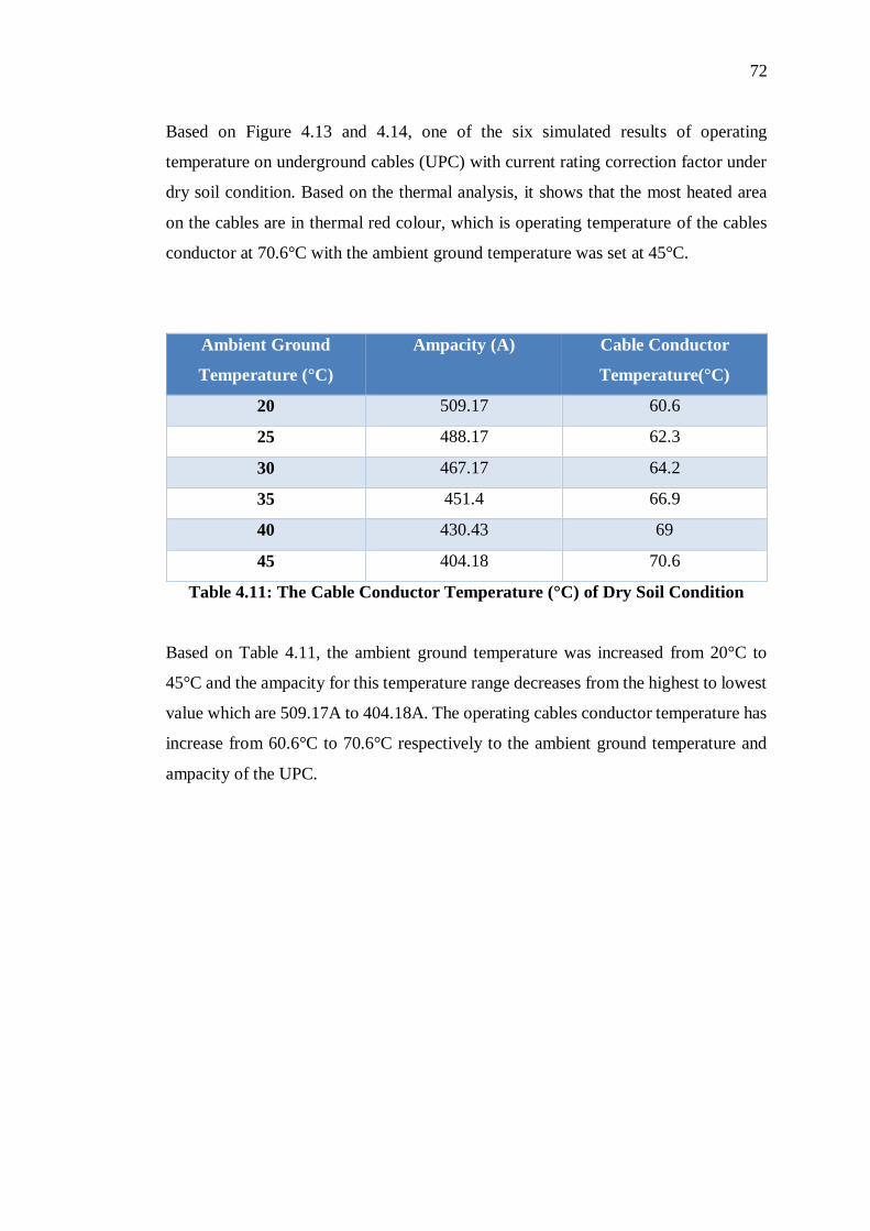
72
Based on Figure 4.13 and 4.14, one of the six simulated results of operating
temperature on underground cables (UPC) with current rating correction factor under
dry soil condition. Based on the thermal analysis, it shows that the most heated area
on the cables are in thermal red colour, which is operating temperature of the cables
conductor at 70.6°C with the ambient ground temperature was set at 45°C.
Ambient Ground
Temperature (°C)
Ampacity (A) Cable Conductor
Temperature(°C)
20 509.17 60.6
25 488.17 62.3
30 467.17 64.2
35 451.4 66.9
40 430.43 69
45 404.18 70.6
Table 4.11: The Cable Conductor Temperature (°C) of Dry Soil Condition
Based on Table 4.11, the ambient ground temperature was increased from 20°C to
45°C and the ampacity for this temperature range decreases from the highest to lowest
value which are 509.17A to 404.18A. The operating cables conductor temperature has
increase from 60.6°C to 70.6°C respectively to the ambient ground temperature and
ampacity of the UPC.
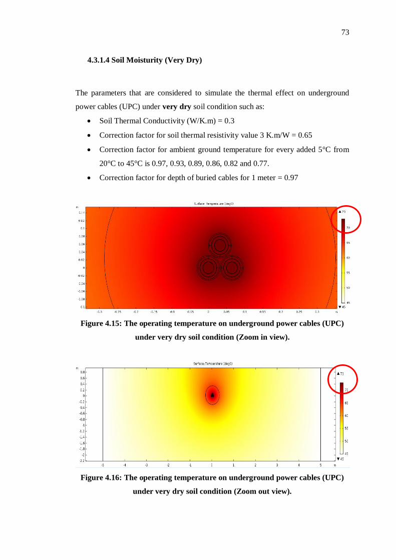
73
4.3.1.4 Soil Moisturity (Very Dry)
The parameters that are considered to simulate the thermal effect on underground
power cables (UPC) under very dry soil condition such as:
Soil Thermal Conductivity (W/K.m) = 0.3
Correction factor for soil thermal resistivity value 3 K.m/W = 0.65
Correction factor for ambient ground temperature for every added 5°C from
20°C to 45°C is 0.97, 0.93, 0.89, 0.86, 0.82 and 0.77.
Correction factor for depth of buried cables for 1 meter = 0.97
Figure 4.15: The operating temperature on underground power cables (UPC)
under very dry soil condition (Zoom in view).
Figure 4.16: The operating temperature on underground power cables (UPC)
under very dry soil condition (Zoom out view).
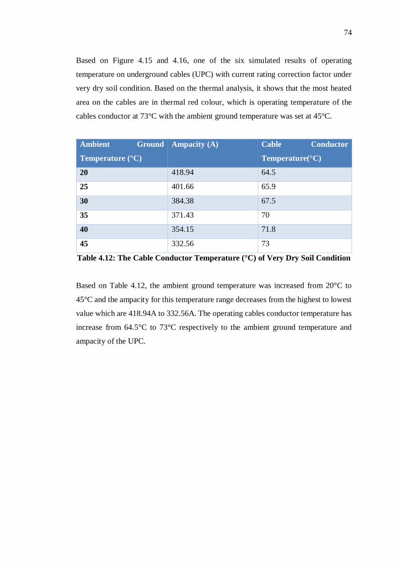
74
Based on Figure 4.15 and 4.16, one of the six simulated results of operating
temperature on underground cables (UPC) with current rating correction factor under
very dry soil condition. Based on the thermal analysis, it shows that the most heated
area on the cables are in thermal red colour, which is operating temperature of the
cables conductor at 73°C with the ambient ground temperature was set at 45°C.
Ambient Ground
Temperature (°C)
Ampacity (A) Cable Conductor
Temperature(°C)
20 418.94 64.5
25 401.66 65.9
30 384.38 67.5
35 371.43 70
40 354.15 71.8
45 332.56 73
Table 4.12: The Cable Conductor Temperature (°C) of Very Dry Soil Condition
Based on Table 4.12, the ambient ground temperature was increased from 20°C to
45°C and the ampacity for this temperature range decreases from the highest to lowest
value which are 418.94A to 332.56A. The operating cables conductor temperature has
increase from 64.5°C to 73°C respectively to the ambient ground temperature and
ampacity of the UPC.
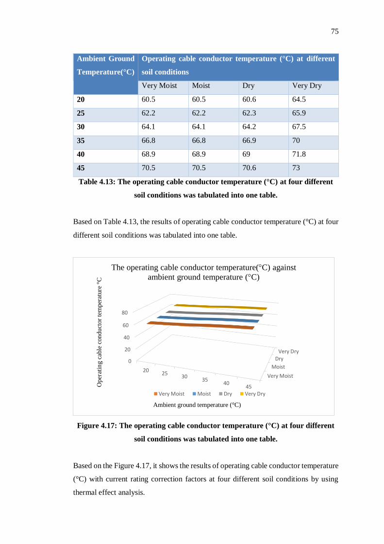
75
Ambient Ground
Temperature(°C)
Operating cable conductor temperature (°C) at different
soil conditions
Very Moist Moist Dry Very Dry
20 60.5 60.5 60.6 64.5
25 62.2 62.2 62.3 65.9
30 64.1 64.1 64.2 67.5
35 66.8 66.8 66.9 70
40 68.9 68.9 69 71.8
45 70.5 70.5 70.6 73
Table 4.13: The operating cable conductor temperature (°C) at four different
soil conditions was tabulated into one table.
Based on Table 4.13, the results of operating cable conductor temperature (°C) at four
different soil conditions was tabulated into one table.
Figure 4.17: The operating cable conductor temperature (°C) at four different
soil conditions was tabulated into one table.
Based on the Figure 4.17, it shows the results of operating cable conductor temperature
(°C) with current rating correction factors at four different soil conditions by using
thermal effect analysis.
Very Moist
Moist
DryVery Dry
0
20
40
60
80
2025
3035
4045
The operating cable conductor temperature(°C) against
ambient ground temperature (°C)
Very Moist Moist Dry Very Dry
Oper
atin
g c
able
con
du
ctor
tem
per
ature
°C
Ambient ground temperature (°C)
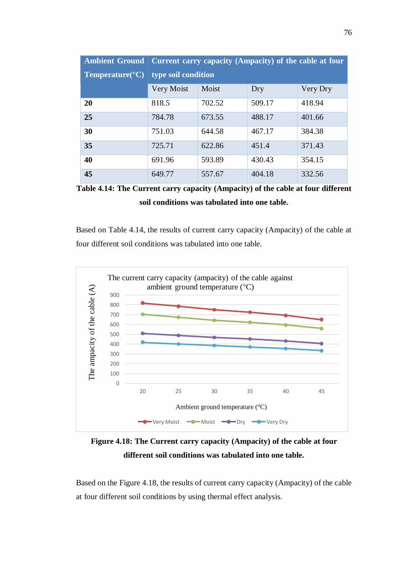
76
Ambient Ground
Temperature(°C)
Current carry capacity (Ampacity) of the cable at four
type soil condition
Very Moist Moist Dry Very Dry
20 818.5 702.52 509.17 418.94
25 784.78 673.55 488.17 401.66
30 751.03 644.58 467.17 384.38
35 725.71 622.86 451.4 371.43
40 691.96 593.89 430.43 354.15
45 649.77 557.67 404.18 332.56
Table 4.14: The Current carry capacity (Ampacity) of the cable at four different
soil conditions was tabulated into one table.
Based on Table 4.14, the results of current carry capacity (Ampacity) of the cable at
four different soil conditions was tabulated into one table.
Figure 4.18: The Current carry capacity (Ampacity) of the cable at four
different soil conditions was tabulated into one table.
Based on the Figure 4.18, the results of current carry capacity (Ampacity) of the cable
at four different soil conditions by using thermal effect analysis.
0
100
200
300
400
500
600
700
800
900
20 25 30 35 40 45
The current carry capacity (ampacity) of the cable against
ambient ground temperature (°C)
Very Moist Moist Dry Very Dry
Ambient ground temperature (°C)
The
am
pacit
y o
f th
e ca
ble
(A
)
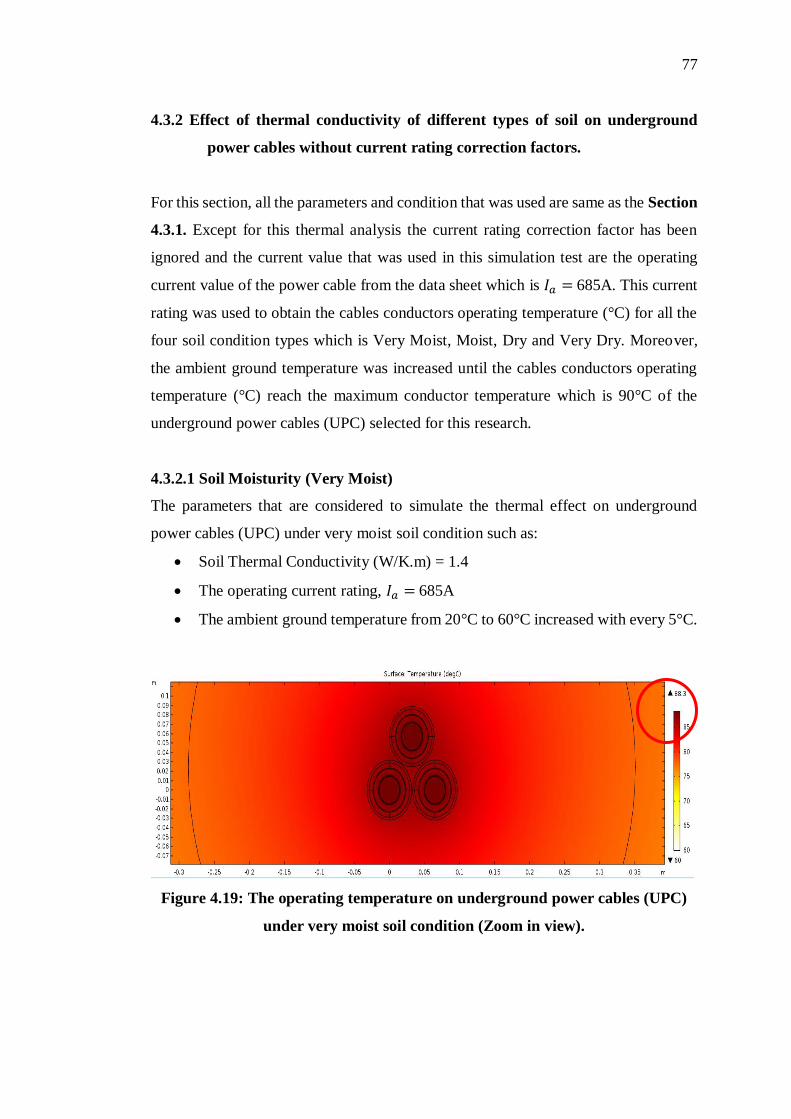
77
4.3.2 Effect of thermal conductivity of different types of soil on underground
power cables without current rating correction factors.
For this section, all the parameters and condition that was used are same as the Section
4.3.1. Except for this thermal analysis the current rating correction factor has been
ignored and the current value that was used in this simulation test are the operating
current value of the power cable from the data sheet which is 𝐼𝑎 = 685A. This current
rating was used to obtain the cables conductors operating temperature (°C) for all the
four soil condition types which is Very Moist, Moist, Dry and Very Dry. Moreover,
the ambient ground temperature was increased until the cables conductors operating
temperature (°C) reach the maximum conductor temperature which is 90°C of the
underground power cables (UPC) selected for this research.
4.3.2.1 Soil Moisturity (Very Moist)
The parameters that are considered to simulate the thermal effect on underground
power cables (UPC) under very moist soil condition such as:
Soil Thermal Conductivity (W/K.m) = 1.4
The operating current rating, 𝐼𝑎 = 685A
The ambient ground temperature from 20°C to 60°C increased with every 5°C.
Figure 4.19: The operating temperature on underground power cables (UPC)
under very moist soil condition (Zoom in view).
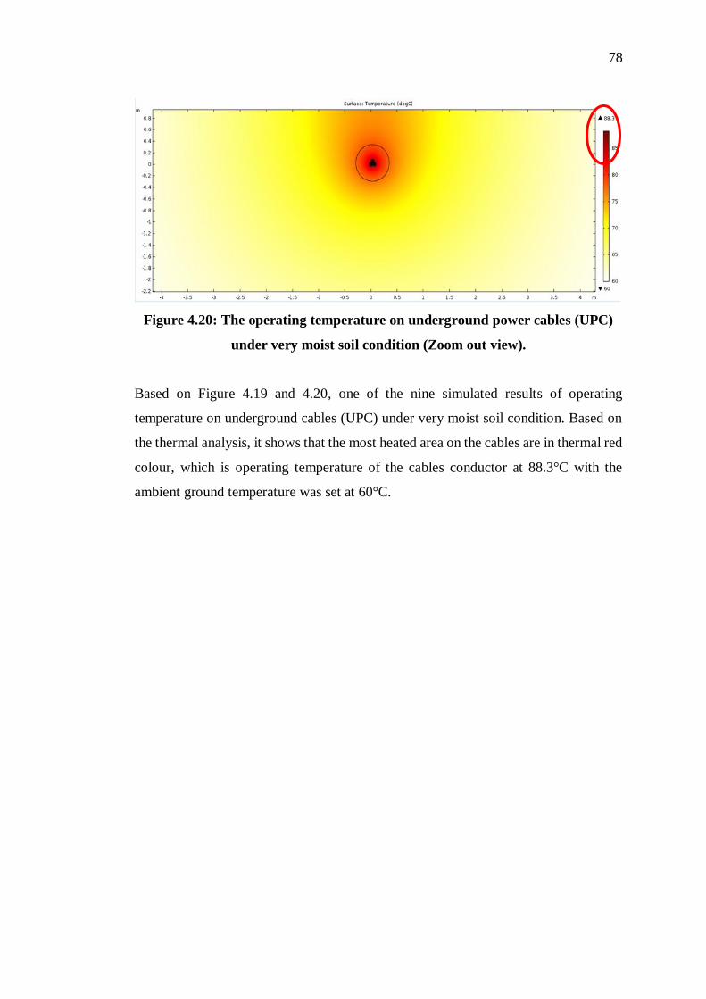
78
Figure 4.20: The operating temperature on underground power cables (UPC)
under very moist soil condition (Zoom out view).
Based on Figure 4.19 and 4.20, one of the nine simulated results of operating
temperature on underground cables (UPC) under very moist soil condition. Based on
the thermal analysis, it shows that the most heated area on the cables are in thermal red
colour, which is operating temperature of the cables conductor at 88.3°C with the
ambient ground temperature was set at 60°C.
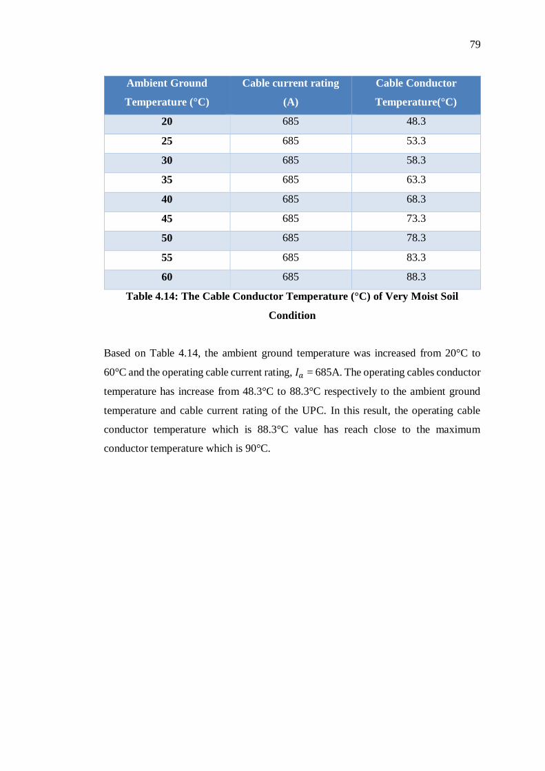
79
Ambient Ground
Temperature (°C)
Cable current rating
(A)
Cable Conductor
Temperature(°C)
20 685 48.3
25 685 53.3
30 685 58.3
35 685 63.3
40 685 68.3
45 685 73.3
50 685 78.3
55 685 83.3
60 685 88.3
Table 4.14: The Cable Conductor Temperature (°C) of Very Moist Soil
Condition
Based on Table 4.14, the ambient ground temperature was increased from 20°C to
60°C and the operating cable current rating, 𝐼𝑎 = 685A. The operating cables conductor
temperature has increase from 48.3°C to 88.3°C respectively to the ambient ground
temperature and cable current rating of the UPC. In this result, the operating cable
conductor temperature which is 88.3°C value has reach close to the maximum
conductor temperature which is 90°C.
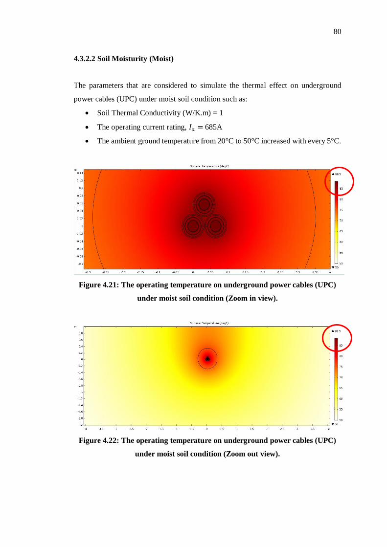
80
4.3.2.2 Soil Moisturity (Moist)
The parameters that are considered to simulate the thermal effect on underground
power cables (UPC) under moist soil condition such as:
Soil Thermal Conductivity (W/K.m) = 1
The operating current rating, 𝐼𝑎 = 685A
The ambient ground temperature from 20°C to 50°C increased with every 5°C.
Figure 4.21: The operating temperature on underground power cables (UPC)
under moist soil condition (Zoom in view).
Figure 4.22: The operating temperature on underground power cables (UPC)
under moist soil condition (Zoom out view).

81
Based on Figure 4.21 and 4.22, one of the seven simulated results of operating
temperature on underground cables (UPC) under moist soil condition. Based on the
thermal analysis, it shows that the most heated area on the cables are in thermal red
colour, which is operating temperature of the cables conductor at 88.5°C with the
ambient ground temperature was set at 50°C.
Ambient Ground
Temperature (°C)
Cable current rating
(A)
Cable Conductor
Temperature(°C)
20 685 58.5
25 685 63.5
30 685 68.5
35 685 73.5
40 685 78.5
45 685 83.5
50 685 88.5
Table 4.15: The Cable Conductor Temperature (°C) of Moist Soil Condition
Based on Table 4.15, the ambient ground temperature was increased from 20°C to
50°C and the operating cable current rating, 𝐼𝑎 = 685A. The operating cables conductor
temperature has increase from 58.5°C to 88.5°C respectively to the ambient ground
temperature and cable current rating of the UPC. In this result, the operating cable
conductor temperature which is 88.5°C value has reach close to the maximum
conductor temperature which is 90°C.
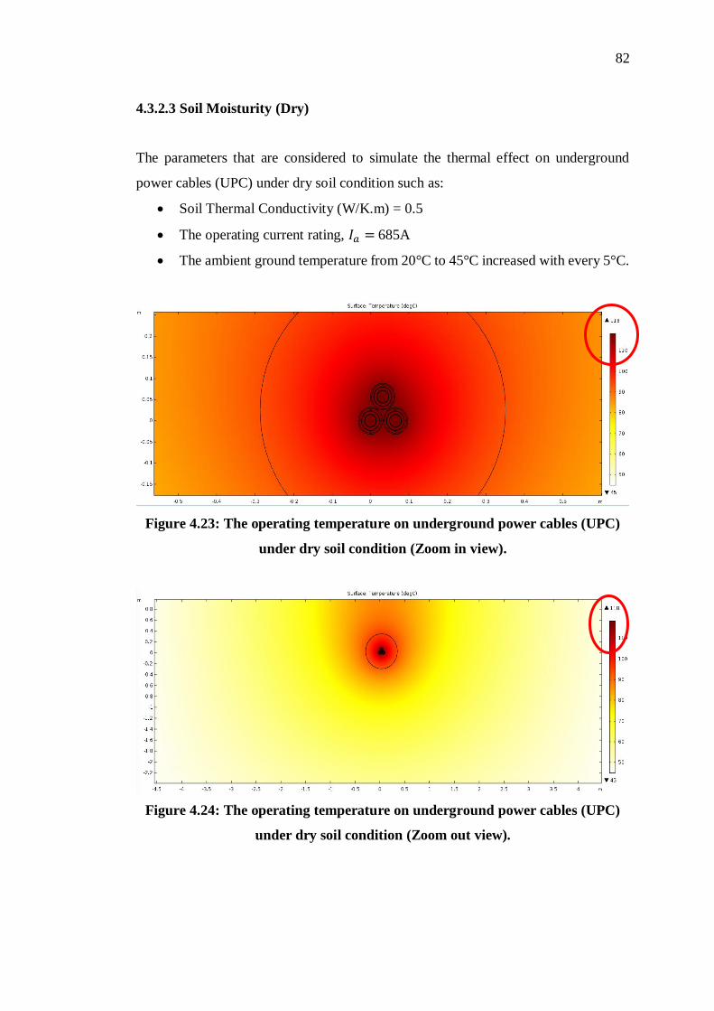
82
4.3.2.3 Soil Moisturity (Dry)
The parameters that are considered to simulate the thermal effect on underground
power cables (UPC) under dry soil condition such as:
Soil Thermal Conductivity (W/K.m) = 0.5
The operating current rating, 𝐼𝑎 = 685A
The ambient ground temperature from 20°C to 45°C increased with every 5°C.
Figure 4.23: The operating temperature on underground power cables (UPC)
under dry soil condition (Zoom in view).
Figure 4.24: The operating temperature on underground power cables (UPC)
under dry soil condition (Zoom out view).
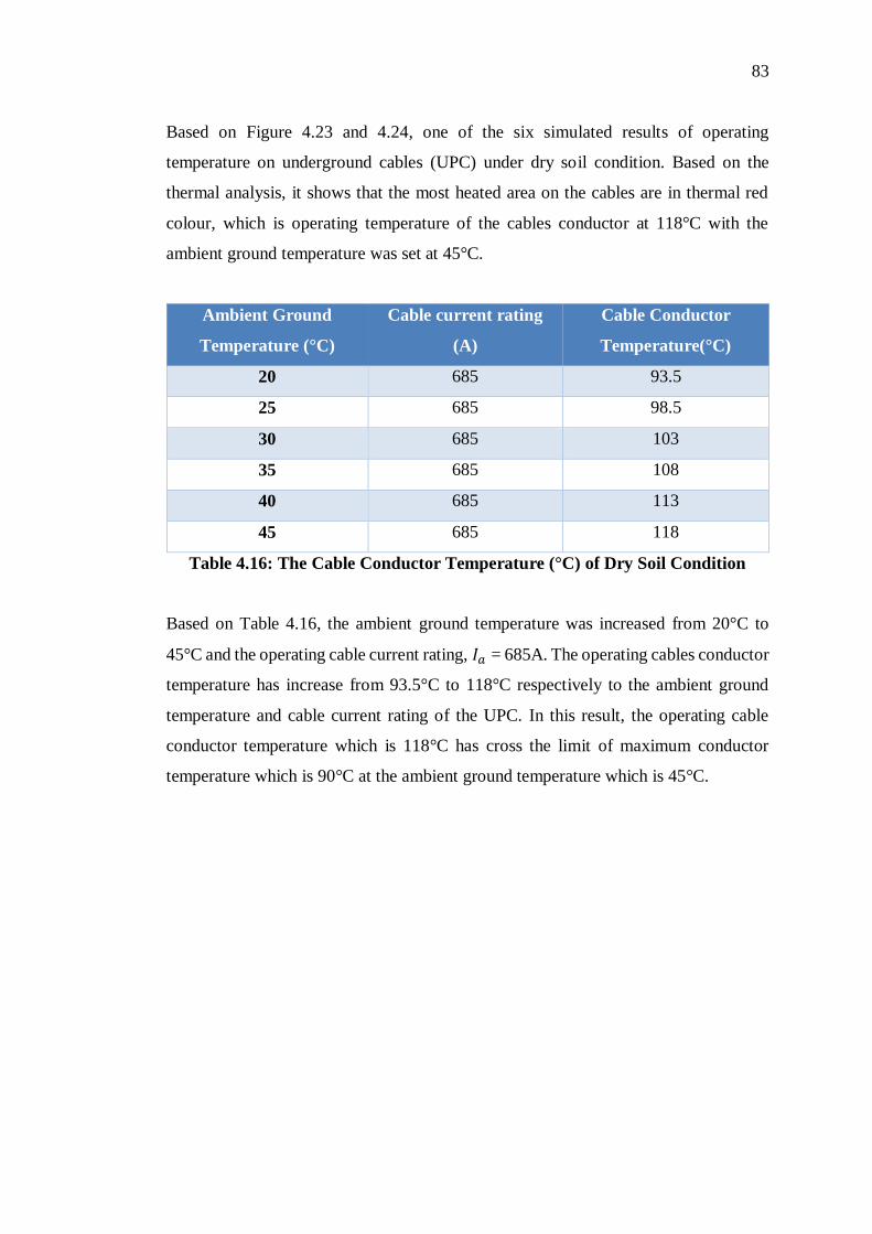
83
Based on Figure 4.23 and 4.24, one of the six simulated results of operating
temperature on underground cables (UPC) under dry soil condition. Based on the
thermal analysis, it shows that the most heated area on the cables are in thermal red
colour, which is operating temperature of the cables conductor at 118°C with the
ambient ground temperature was set at 45°C.
Ambient Ground
Temperature (°C)
Cable current rating
(A)
Cable Conductor
Temperature(°C)
20 685 93.5
25 685 98.5
30 685 103
35 685 108
40 685 113
45 685 118
Table 4.16: The Cable Conductor Temperature (°C) of Dry Soil Condition
Based on Table 4.16, the ambient ground temperature was increased from 20°C to
45°C and the operating cable current rating, 𝐼𝑎 = 685A. The operating cables conductor
temperature has increase from 93.5°C to 118°C respectively to the ambient ground
temperature and cable current rating of the UPC. In this result, the operating cable
conductor temperature which is 118°C has cross the limit of maximum conductor
temperature which is 90°C at the ambient ground temperature which is 45°C.
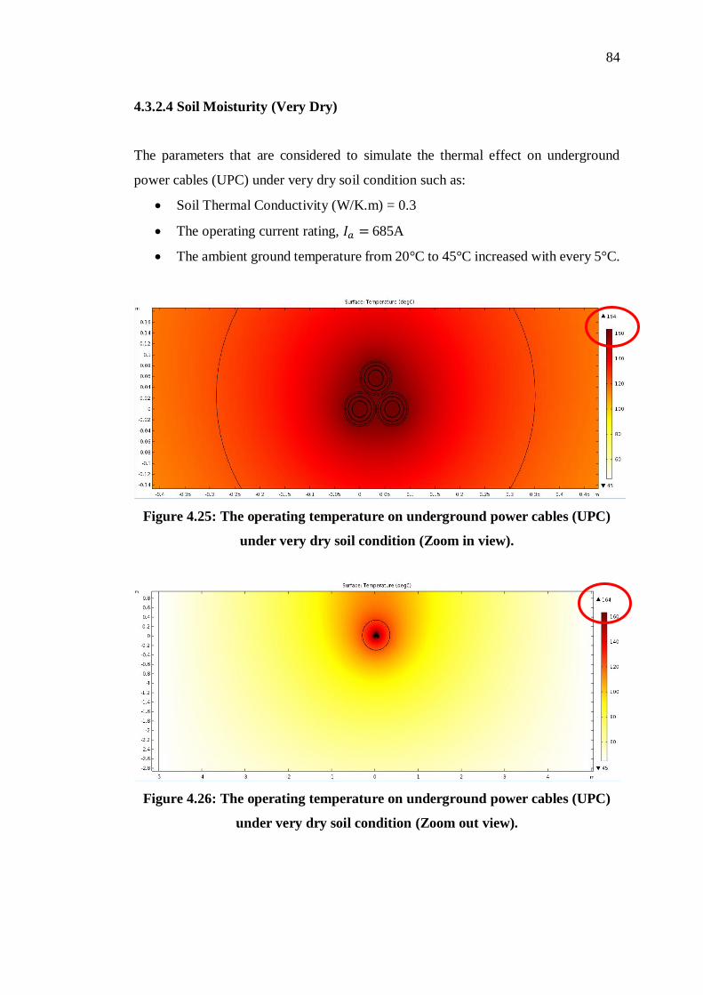
84
4.3.2.4 Soil Moisturity (Very Dry)
The parameters that are considered to simulate the thermal effect on underground
power cables (UPC) under very dry soil condition such as:
Soil Thermal Conductivity (W/K.m) = 0.3
The operating current rating, 𝐼𝑎 = 685A
The ambient ground temperature from 20°C to 45°C increased with every 5°C.
Figure 4.25: The operating temperature on underground power cables (UPC)
under very dry soil condition (Zoom in view).
Figure 4.26: The operating temperature on underground power cables (UPC)
under very dry soil condition (Zoom out view).
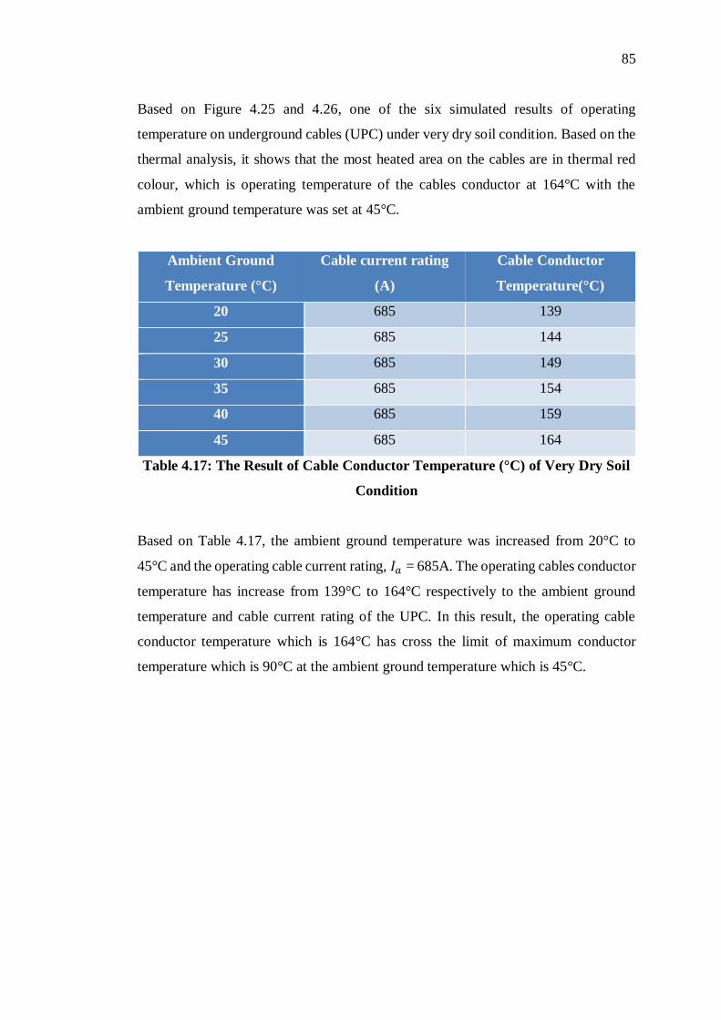
85
Based on Figure 4.25 and 4.26, one of the six simulated results of operating
temperature on underground cables (UPC) under very dry soil condition. Based on the
thermal analysis, it shows that the most heated area on the cables are in thermal red
colour, which is operating temperature of the cables conductor at 164°C with the
ambient ground temperature was set at 45°C.
Ambient Ground
Temperature (°C)
Cable current rating
(A)
Cable Conductor
Temperature(°C)
20 685 139
25 685 144
30 685 149
35 685 154
40 685 159
45 685 164
Table 4.17: The Result of Cable Conductor Temperature (°C) of Very Dry Soil
Condition
Based on Table 4.17, the ambient ground temperature was increased from 20°C to
45°C and the operating cable current rating, 𝐼𝑎 = 685A. The operating cables conductor
temperature has increase from 139°C to 164°C respectively to the ambient ground
temperature and cable current rating of the UPC. In this result, the operating cable
conductor temperature which is 164°C has cross the limit of maximum conductor
temperature which is 90°C at the ambient ground temperature which is 45°C.
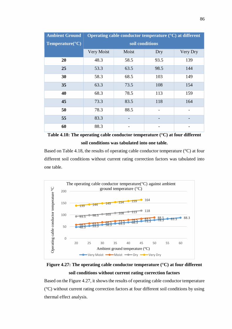
86
Ambient Ground
Temperature(°C)
Operating cable conductor temperature (°C) at different
soil conditions
Very Moist Moist Dry Very Dry
20 48.3 58.5 93.5 139
25 53.3 63.5 98.5 144
30 58.3 68.5 103 149
35 63.3 73.5 108 154
40 68.3 78.5 113 159
45 73.3 83.5 118 164
50 78.3 88.5 - -
55 83.3 - - -
60 88.3 - - -
Table 4.18: The operating cable conductor temperature (°C) at four different
soil conditions was tabulated into one table.
Based on Table 4.18, the results of operating cable conductor temperature (°C) at four
different soil conditions without current rating correction factors was tabulated into
one table.
Figure 4.27: The operating cable conductor temperature (°C) at four different
soil conditions without current rating correction factors
Based on the Figure 4.27, it shows the results of operating cable conductor temperature
(°C) without current rating correction factors at four different soil conditions by using
thermal effect analysis.
48.3 53.3 58.3 63.3 68.3 73.3 78.3 83.3 88.3
58.5 63.5 68.5 73.5 78.5 83.5 88.593.5 98.5 103 108 113 118
139 144 149 154 159 164
0
50
100
150
200
20 25 30 35 40 45 50 55 60
The operating cable conductor temperature(°C) against ambient ground temperature (°C)
Very Moist Moist Dry Very Dry
Ambient ground temperature (°C)
Op
erat
ing c
able
con
du
ctor
tem
per
ature
°C
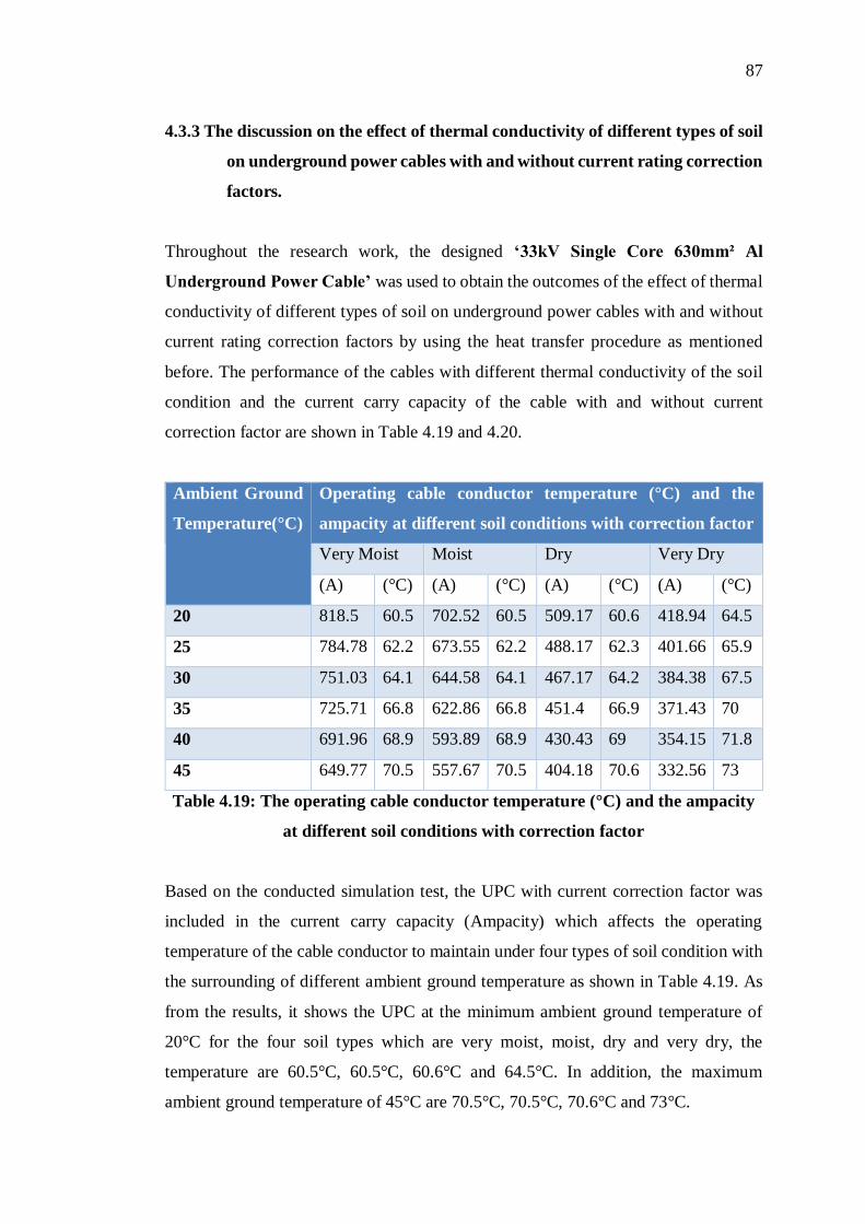
87
4.3.3 The discussion on the effect of thermal conductivity of different types of soil
on underground power cables with and without current rating correction
factors.
Throughout the research work, the designed ‘33kV Single Core 630mm² Al
Underground Power Cable’ was used to obtain the outcomes of the effect of thermal
conductivity of different types of soil on underground power cables with and without
current rating correction factors by using the heat transfer procedure as mentioned
before. The performance of the cables with different thermal conductivity of the soil
condition and the current carry capacity of the cable with and without current
correction factor are shown in Table 4.19 and 4.20.
Ambient Ground
Temperature(°C)
Operating cable conductor temperature (°C) and the
ampacity at different soil conditions with correction factor
Very Moist Moist Dry Very Dry
(A) (°C) (A) (°C) (A) (°C) (A) (°C)
20 818.5 60.5 702.52 60.5 509.17 60.6 418.94 64.5
25 784.78 62.2 673.55 62.2 488.17 62.3 401.66 65.9
30 751.03 64.1 644.58 64.1 467.17 64.2 384.38 67.5
35 725.71 66.8 622.86 66.8 451.4 66.9 371.43 70
40 691.96 68.9 593.89 68.9 430.43 69 354.15 71.8
45 649.77 70.5 557.67 70.5 404.18 70.6 332.56 73
Table 4.19: The operating cable conductor temperature (°C) and the ampacity
at different soil conditions with correction factor
Based on the conducted simulation test, the UPC with current correction factor was
included in the current carry capacity (Ampacity) which affects the operating
temperature of the cable conductor to maintain under four types of soil condition with
the surrounding of different ambient ground temperature as shown in Table 4.19. As
from the results, it shows the UPC at the minimum ambient ground temperature of
20°C for the four soil types which are very moist, moist, dry and very dry, the
temperature are 60.5°C, 60.5°C, 60.6°C and 64.5°C. In addition, the maximum
ambient ground temperature of 45°C are 70.5°C, 70.5°C, 70.6°C and 73°C.

88
This proves that the given correction factors from the cable datasheet are to prevent
the operating temperature of the cable to reach the maximum operating temperature of
conductor which is 90°C from any circumstances. Basically, when more conductors of
the cables are energized, there will be high rate of heat will be produced so the
excessive amount of heat generated within the conductors are compensated by using
the current rating correction factors.
Ambient Ground
Temperature(°C)
Operating cable conductor temperature (°C) and the
ampacity at different soil conditions without correction
factor
Very Moist Moist Dry Very Dry
(A) (°C) (A) (°C) (A) (°C) (A) (°C)
20 685 48.3 685 58.5 685 93.5 685 139
25 685 53.3 685 63.5 685 98.5 685 144
30 685 58.3 685 68.5 685 103 685 149
35 685 63.3 685 73.5 685 108 685 154
40 685 68.3 685 78.5 685 113 685 159
45 685 73.3 685 83.5 685 118 685 164
Table 4.20: The operating cable conductor temperature (°C) and the ampacity
at different soil conditions without correction factor
After that, a second test was conducted on the UPC without including current rating
correction factor and the current was fixed at 685A as shown in Table 4.20. This affects
the operating temperature of the cable conductor to increase for the dry and very dry
soil condition to extremely high by crossing the limit of the maximum conductor
temperature of the cable with different ambient ground temperature. As from the result,
it shows that the UPC at the minimum ambient ground temperature at 20°C for dry
and very dry soil type, the temperature are 93.5°C and 139°C. In addition, the
maximum ambient ground temperature at 45°C are 118°C and 164°C. Besides that,
the operating temperature of cable conductor of the other two soil type very moist and
moist are basically lower than the maximum temperature of the conductor at the
minimum ambient ground temperature at 20°C, the operating cable conductor
89
temperature are 48.3°C, 58.5°C and for maximum ambient ground temperature at 45°C,
the operating cable conductor temperature are 73.3°C and 83.5°C.
This results shows that without implementing the correction factor into the cables, the
operating temperature of the cable conductors will be affected by ambient ground
temperature respectively with the soil thermal conductivity and soil resistivity. Since
the soil thermal conductivity of the dry and very dry which is 0.5 W/K.m and 0.3
W/K.m, the heat from the operating cables will be dispersed slowly to surrounding
ground so this will increase the temperature of the cable conductors. Basically, this are
the main reasons behind where the cables temperature increases.
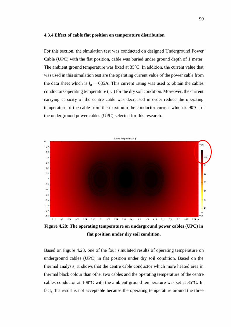
90
4.3.4 Effect of cable flat position on temperature distribution
For this section, the simulation test was conducted on designed Underground Power
Cable (UPC) with the flat position, cable was buried under ground depth of 1 meter.
The ambient ground temperature was fixed at 35°C. In addition, the current value that
was used in this simulation test are the operating current value of the power cable from
the data sheet which is 𝐼𝑎 = 685A. This current rating was used to obtain the cables
conductors operating temperature (°C) for the dry soil condition. Moreover, the current
carrying capacity of the centre cable was decreased in order reduce the operating
temperature of the cable from the maximum the conductor current which is 90°C of
the underground power cables (UPC) selected for this research.
Figure 4.28: The operating temperature on underground power cables (UPC) in
flat position under dry soil condition.
Based on Figure 4.28, one of the four simulated results of operating temperature on
underground cables (UPC) in flat position under dry soil condition. Based on the
thermal analysis, it shows that the centre cable conductor which more heated area in
thermal black colour than other two cables and the operating temperature of the centre
cables conductor at 108°C with the ambient ground temperature was set at 35°C. In
fact, this result is not acceptable because the operating temperature around the three
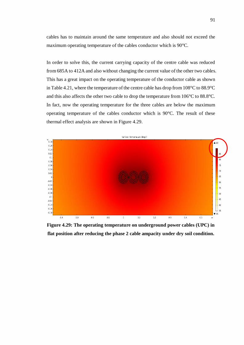
91
cables has to maintain around the same temperature and also should not exceed the
maximum operating temperature of the cables conductor which is 90°C.
In order to solve this, the current carrying capacity of the centre cable was reduced
from 685A to 412A and also without changing the current value of the other two cables.
This has a great impact on the operating temperature of the conductor cable as shown
in Table 4.21, where the temperature of the centre cable has drop from 108°C to 88.9°C
and this also affects the other two cable to drop the temperature from 106°C to 88.8°C.
In fact, now the operating temperature for the three cables are below the maximum
operating temperature of the cables conductor which is 90°C. The result of these
thermal effect analysis are shown in Figure 4.29.
Figure 4.29: The operating temperature on underground power cables (UPC) in
flat position after reducing the phase 2 cable ampacity under dry soil condition.
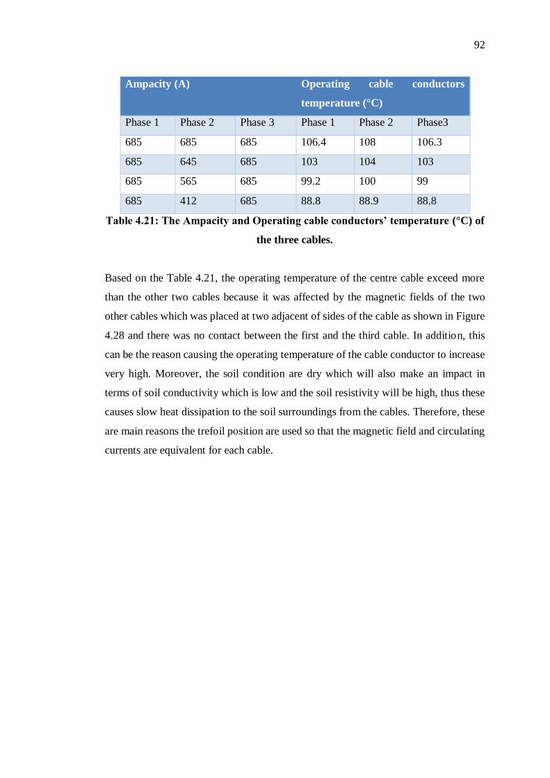
92
Ampacity (A) Operating cable conductors
temperature (°C)
Phase 1 Phase 2 Phase 3 Phase 1 Phase 2 Phase3
685 685 685 106.4 108 106.3
685 645 685 103 104 103
685 565 685 99.2 100 99
685 412 685 88.8 88.9 88.8
Table 4.21: The Ampacity and Operating cable conductors’ temperature (°C) of
the three cables.
Based on the Table 4.21, the operating temperature of the centre cable exceed more
than the other two cables because it was affected by the magnetic fields of the two
other cables which was placed at two adjacent of sides of the cable as shown in Figure
4.28 and there was no contact between the first and the third cable. In addition, this
can be the reason causing the operating temperature of the cable conductor to increase
very high. Moreover, the soil condition are dry which will also make an impact in
terms of soil conductivity which is low and the soil resistivity will be high, thus these
causes slow heat dissipation to the soil surroundings from the cables. Therefore, these
are main reasons the trefoil position are used so that the magnetic field and circulating
currents are equivalent for each cable.
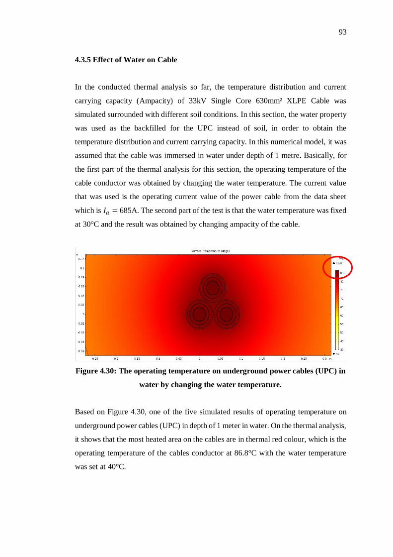
93
4.3.5 Effect of Water on Cable
In the conducted thermal analysis so far, the temperature distribution and current
carrying capacity (Ampacity) of 33kV Single Core 630mm² XLPE Cable was
simulated surrounded with different soil conditions. In this section, the water property
was used as the backfilled for the UPC instead of soil, in order to obtain the
temperature distribution and current carrying capacity. In this numerical model, it was
assumed that the cable was immersed in water under depth of 1 metre. Basically, for
the first part of the thermal analysis for this section, the operating temperature of the
cable conductor was obtained by changing the water temperature. The current value
that was used is the operating current value of the power cable from the data sheet
which is 𝐼𝑎 = 685A. The second part of the test is that the water temperature was fixed
at 30°C and the result was obtained by changing ampacity of the cable.
Figure 4.30: The operating temperature on underground power cables (UPC) in
water by changing the water temperature.
Based on Figure 4.30, one of the five simulated results of operating temperature on
underground power cables (UPC) in depth of 1 meter in water. On the thermal analysis,
it shows that the most heated area on the cables are in thermal red colour, which is the
operating temperature of the cables conductor at 86.8°C with the water temperature
was set at 40°C.
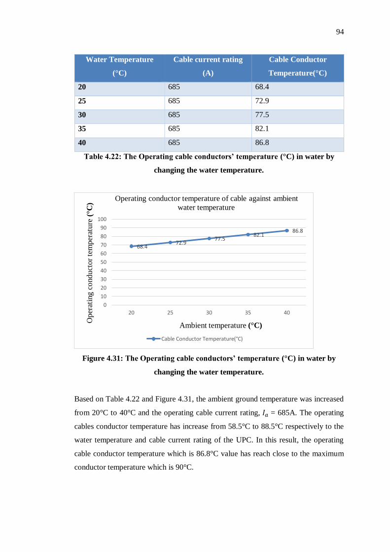
94
Water Temperature
(°C)
Cable current rating
(A)
Cable Conductor
Temperature(°C)
20 685 68.4
25 685 72.9
30 685 77.5
35 685 82.1
40 685 86.8
Table 4.22: The Operating cable conductors’ temperature (°C) in water by
changing the water temperature.
Figure 4.31: The Operating cable conductors’ temperature (°C) in water by
changing the water temperature.
Based on Table 4.22 and Figure 4.31, the ambient ground temperature was increased
from 20°C to 40°C and the operating cable current rating, 𝐼𝑎 = 685A. The operating
cables conductor temperature has increase from 58.5°C to 88.5°C respectively to the
water temperature and cable current rating of the UPC. In this result, the operating
cable conductor temperature which is 86.8°C value has reach close to the maximum
conductor temperature which is 90°C.
68.472.9
77.582.1
86.8
0
10
20
30
40
50
60
70
80
90
100
20 25 30 35 40
Operating conductor temperature of cable against ambient
water temperature
Cable Conductor Temperature(°C)
Ambient temperature (°C)
Oper
atin
g c
onduct
or
tem
per
ature
(°C
)
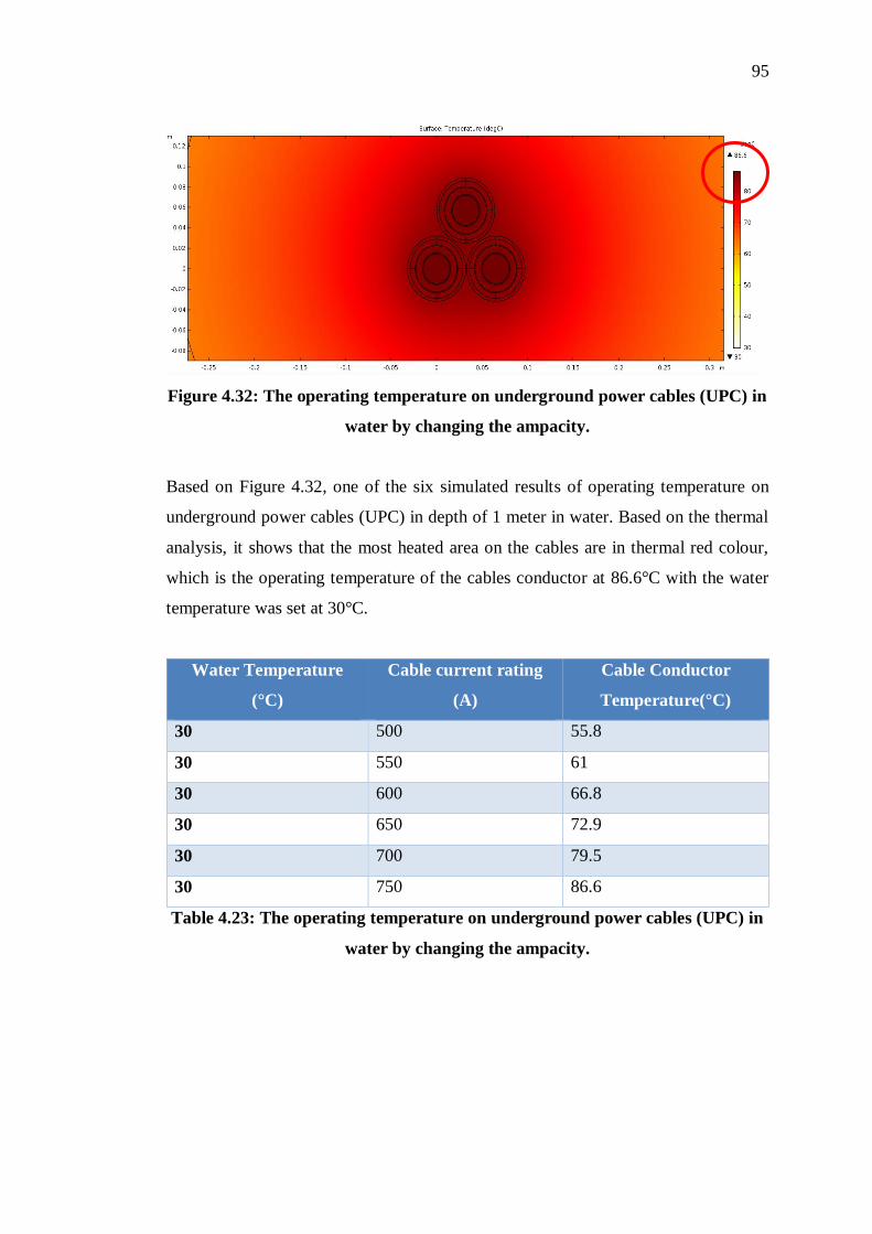
95
Figure 4.32: The operating temperature on underground power cables (UPC) in
water by changing the ampacity.
Based on Figure 4.32, one of the six simulated results of operating temperature on
underground power cables (UPC) in depth of 1 meter in water. Based on the thermal
analysis, it shows that the most heated area on the cables are in thermal red colour,
which is the operating temperature of the cables conductor at 86.6°C with the water
temperature was set at 30°C.
Water Temperature
(°C)
Cable current rating
(A)
Cable Conductor
Temperature(°C)
30 500 55.8
30 550 61
30 600 66.8
30 650 72.9
30 700 79.5
30 750 86.6
Table 4.23: The operating temperature on underground power cables (UPC) in
water by changing the ampacity.

96
Figure 4.33: The operating temperature on underground power cables (UPC) in
water by changing the ampacity.
Based on Table 4.23 and Figure 4.33, the water temperature was set at 30°C and the
ampacity of the cable was increased from 500A to 750A. The operating cables
conductor temperature has increase from 55.8°C to 86.6°C respectively to the water
temperature and cable current rating of the UPC. In this result, the operating cable
conductor temperature which is 86.6°C value has reach close to the maximum
conductor temperature which is 90°C.
Basically, by comparing both simulation test result on the operating temperature of the
cable conductor was obtained by changing the water temperature and current carrying
capacity of the UPC which shows that the operating temperature of the cable conductor
in water surrounding are higher than the soil surrounding. This factor can be
experienced because the heat from the cables are dispersed slowly into the water
surrounding than the soil surrounding. In fact, the thermal conductivity of the water
can be one of the reason for the heating factor because it changes respectively with the
water ambient temperature. Besides that, this selected 33kV XLPE Single Core Al
630mm² cable are not suitable to operate underwater. Basically, if there any deep
damages occurs on the cable’s PVC insulation, the water will flow into the cables
which causes the temperature to rise and in result it will explode. In matter of fact, the
55.861
66.872.9
79.586.6
0
10
20
30
40
50
60
70
80
90
100
500 550 600 650 700 750
Operating temperature of Cable Conductor
Temperature(°C) against Ampacity (A)
Cable Conductor Temperature(°C)
Op
erati
ng c
ondu
ctor
tem
per
atu
re (°C
)
Ampacity (A)

97
most suitable cable to operate under water is the ‘submarine cable’ where it was
specially made to carry the current in water surrounded area.
4.4 Summary
In brief, the thermal analysis was conducted on the “33kV Single Core 630mm²
Al XLPE Cable. Firstly, the thermal effect on the single underground power cable
(UPC) was studied and analysed by changing the buried depth of the cable thus laying
the single core cable in depth of 1 meter will be the preferred depth for the cable than
the 0.5 meter depth and this was proven by comparing the results of the operating cable
conductor’s temperature in two different depth. Secondly, the Trefoil position of UPC
was studied and analysed in different soil condition, different ground ambient
temperature and also with and without the current rating correction factor. In matter of
fact, the given correction factors from the cable datasheet are to prevent the operating
temperature of the cables from reaching the maximum conductor temperature which
are 90°C. On the other hand, ignoring the correction factors from cables causes the
operating temperature of the cable conductor to be affected by the ambient ground
temperature respectively with the soil thermal conductivity and resistivity. Thirdly, the
operating conductor temperature of UPC in flat position was studied and analysed by
changing the ampacity of the cables thus the operating temperature of the centre cable
exceed more than the other two cable because it was affected by the magnetic fields of
the two other cables which was placed at two adjacent of sides of the cable. Finally,
the operating conductor temperature of UPC in immersed in water was also studied
and analysed. In fact, the operating temperature of the cable conductor was obtained
by changing the water temperature and current carrying capacity of the UPC, which
shows that the operating temperature of the cable conductor in water environment are
higher than the of soil environment due to the heat from cable are slowly dispersed
into the water surrounding than the soil surrounding due to the thermal conductivity of
the water which can be the reason for the heating factor.
98
CHAPTER 5
1 CONCLUSIONS AND RECOMMENDATIONS
5.1 Conclusion
In the nutshell, the purpose of this project has create a good progress on the
combination section, succeeding the aim and objectives as stated in Section 1.3, which
focused more on to designed and analysed the Thermal Effect on the Underground
Power Cable, to do some studies on chosen 33KV Single Core 1x630mm² XLPE Cable,
studied the FEM by using COMSOL software, studied the effect thermal conductivity
of the soil condition on underground power cable (UPC), the cable laying position of
the cables, effect of different burial depth of the cable and also studied the thermal
effect on the cable by using water as surrounding material. The main purpose of this
analysis was conducted in order to study and record the temperature distribution on
the underground power cable (UPC) and also to determine the current passing through
the cable with and without current rating correction factor. Through the reference and
instruction accessible from online sources, learning and understand the COMSOL
software, learn about the underground power cable were to a certain extent it’s really
challenging and lots of knowledge has been gain throughout the learning process.
In fact, by achieving all the aim and objective as stated in Section 1.3, there are number
of benefits have been earned from this research such as:
The effectiveness of using different material as backfill of the cable.
The effect of laying the cable under the soil by choosing the best position of the
cable.
The operating temperature of the cable can be measured by using the software with
sufficient information.
The operating cable conductor temperature will be more stable by including the
current rating correction factor.
99
5.2 Recommendations
In this project, there is room for improvements can make from this studies. Since, the
finite element method (FEM) with the COMSOL software has been used to analyse
and study the thermal effect on underground cable has been succeeded. The next step
can be developed by using this knowledge is to study and analyse ‘The Thermal Effect
of Underground Cable Joints’. Usually, if the distribution line is more than 500 meters
then there will be cable jointed for every 500 meters thus this will be very helpful to
study the cause of the cable breakdown that occurs on the cable jointing part.
Furthermore, the effect thermal conductivity of the soil condition on underground
cable joints, the effect of cable joint position/arrangement, effect of different burial
depth of the cable joint, immersed the cable joint under water can be studied and
analysed by using the FEM with the COMSOL software.
100
REFERENCES
ANIXER. (2018). Retrieved from Copper vs. Aluminum Conductors:
https://www.anixter.com/en_uk/resources/literature/wire-wisdom/copper-vs-
aluminum-conductors.html [Accessed 11 April 2019].
BSE Border States-Supply Chain Solutions. (2014, May 29). Retrieved from Copper
vs. Aluminum Cable and Copper Coatings: Their Best Use Cases:
https://solutions.borderstates.com/copper-vs-aluminum-cable-and-copper-coatings-
their-best-use-cases/ [Accessed 11 April 2019].
Edvard. (2010, December 12). EEP-Electrical Engineering Portal. Retrieved from
Sheilding of Power Cables: https://electrical-engineering-portal.com/shielding-of-
power-cables [Accessed 11 April 2019].
Edvard. (2014, November 12). EEP-Electrical Engineering Portal. Retrieved from
Characteristics of XLPE insulated cables: https://electrical-engineering-
portal.com/characteristics-of-xlpe-insulated-cables-with-reference-to-the-uk-
standards [Accessed 11 April 2019].
ELAND CABLES. (2019). Retrieved from WHAT ARE THE BENEFITS OF PVC
INSULATED CABLES?: https://www.elandcables.com/the-cable-lab/faqs/faq-what-
are-the-benefits-of-pvc-insulated-cables [Accessed 11 April 2019].
Hwang, C. C. (2003). "Extensions to the finite element method for thermal. Elsevier
Electric Power Systems Research, 159-164.

101
Igwe, O. E. (2016). Cable Sizing and Its Effect on Thermal and Ampacity Values in
Underground Power Distribution. University of kentuky UKnowledge, 43.
Kalenderli, M. K. (n.d.). Coupled Electrical and Thermal Analysis of Power Cables
Using Finite Element Method. Heat Transfer – Engineering Applications, pp. 206-
227.
Kocar, I. E. (2004). Thermal analysis for determination of current carrying capacityof
PE and XLPE insulated power cables using finite element method. IEEE MELECON,
905-908.
Littmarck, S. (2015, NOVEMBER 20). COMSOL. Retrieved from COMSOL
MODELING SOFTWARE: https://www.comsol.com/ [Accessed 11 April 2019].
M. Rasoulpoor, M. M. (2016). Electromagnetic and thermal analysis of
undergroundpower solid‐conductor cables under harmonic andunbalancing currents
based on FEM. Wiley, 1-17 .
Monika Rerak, P. O. (2017). The effect of soil and cable backfill thermal conductivity
on the. E3S Web of Conferences WTiUE 201 6, 1-5.
Murat Karahan, H. S. (2009). Thermal Analysis of Power Cables Using Finite Element
Method and Current-carrying Capacity Evaluation. International Journal of
Engineering Education, 2-7.
Parmar, J. (2016, April 7). Electrical Notes & Articles. Retrieved from Cable
Construction & Cable Selection- Part:1:
https://electricalnotes.wordpress.com/2016/04/07/cable-construction-cable-selection-
part1/ [Accessed 11 April 2019].
Tedas (Turkish Electrical Power Distribution Inc.). (2005). Assembly (application)
principlesand guidelines for power cables in the electrical power distribution
networks. Retrieved from istanbul.meteor.gov.tr/marmaraiklimi.htm
102
1 APPENDICES
APPENDIX A: XLPE INSULATED POWER & IEC STANDARDS (CENTRAL
CABLES BERHAD (7169-A)
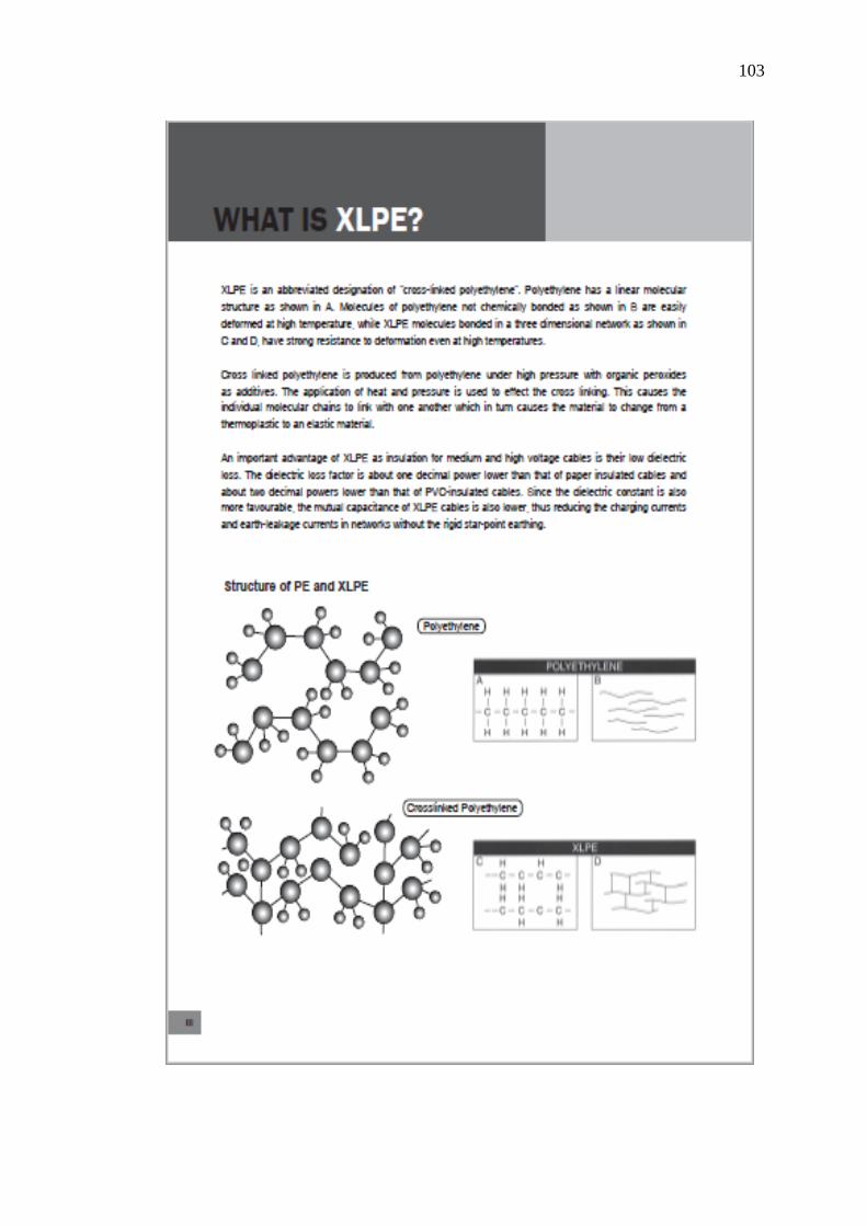
103
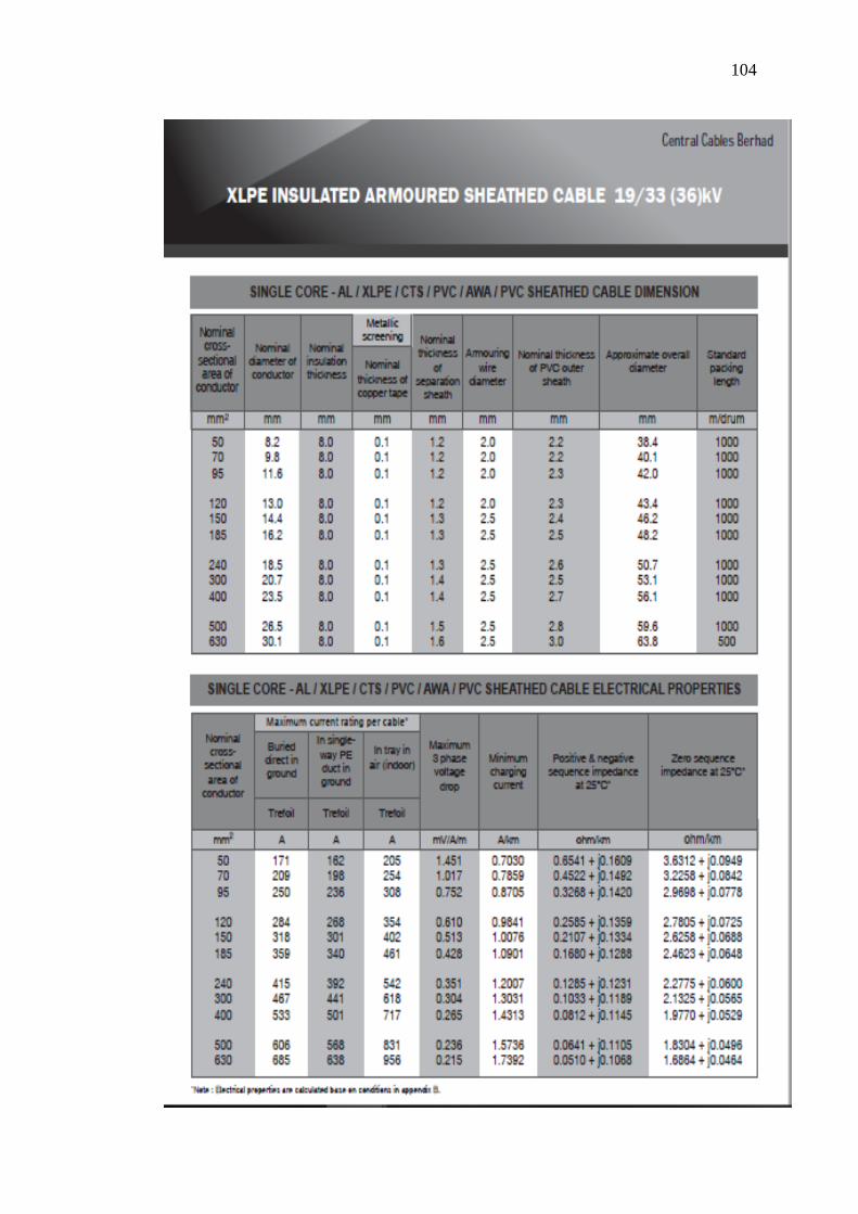
104
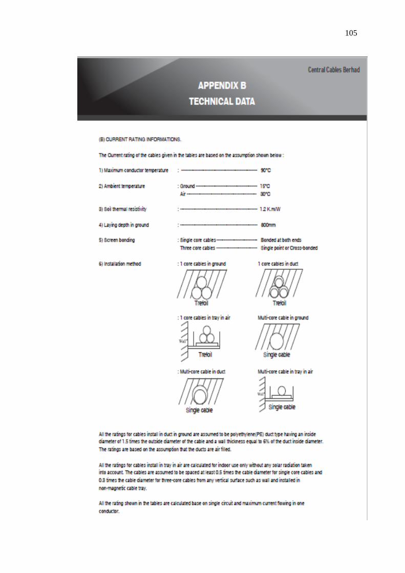
105
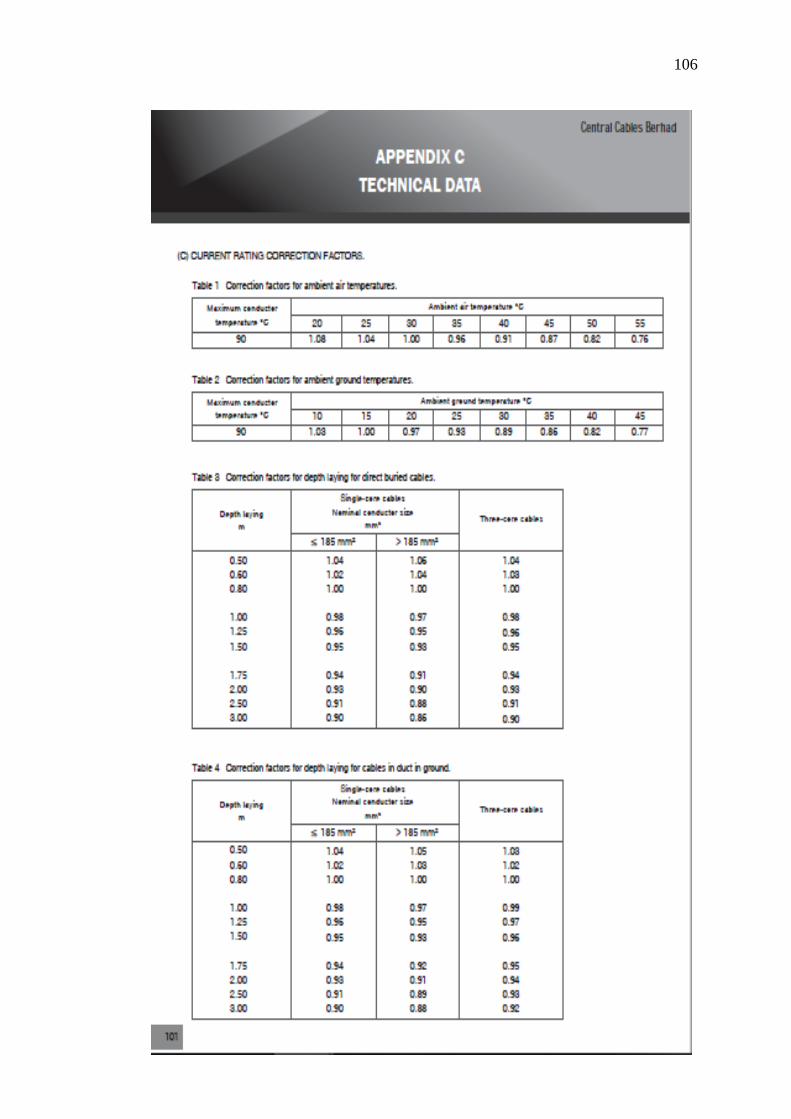
106
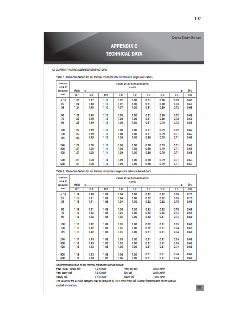
107