CUN. CHEM. 21/2, 249-254(1975)

CLINICALCHEMISTRY,Vol. 21, No. 2, 1975 249

Theory of Photometric Errors Applied to the Design and

Evaluation of a High-Performance Filter Photometer

Thomas E. Hewitt1 and Harry L. Pardue2

We have applied a comprehensive theory of photomet-ric errors to the design and evaluation of an inexpensivestabilized photometer. The photometer is described interms of a group of modules, the characteristics ofwhich are described in terms of their effect on specificerror coefficients. Procedures described in this papershow how the principles described earlier [Clin. Chem.20, 1028 (1974)] can be used to optimize the design ofnew instrumentation or to evaluate the performance ofexisting instrumentation. Chemical data are included toverify the agreement between predicted and experi-mental results.

There is continuing interest in improved reliabilityin analytical methods used in clinical chemistry (1).Because a large percentage of all clinical analyses arebased on photometric measurements (2), there isstrong motivation both to develop photometric sys-tems that have negligible errors inherent in the in-strument and (or) to use such systems in a mannersuch that the unavoidable instrumental errors willmake minimal contributions to the uncertainty in thechemical analysis. In a recent paper we describedmathematical procedures for the evaluation and in-terpretation of photometric errors as they apply toequilibrium and kinetic analyses (3). While that re-port included a comprehensive treatment of differenttypes of errors, it did not include a very complete dis-cussion of how the procedures are applied to real sys-

Department of Chemistry, Purdue University, Lafayette, led.47907.

1 Present address: University Hospitals, University of Wiscon-

sin, Madison, Wis. 53706.2Correspondence should be addressed to this author.

Received Oct. 11, 1974; accepted Nov. 25, 1974.

tems. In this paper we show how we have used ourmathematical procedures in the design and evalua-tion of a high performance filter photometer. Be-cause the photometer has some attractive featuresthat result from design concepts not reported pre-viously, we have included details of the photometerdesign.

In our earlier paper (3), we assumed that the totalrandom error in an absorbance measurement is com-posed of the sum of three error components

v’#{176}\2 (pQo \2 (1 /20o \2

S - 0 434 ‘ T.OI “ T.1/ + \ T.1/21A- - r

where SA is the standard deviation of the absorbancemeasurement, T is the transmittance, and S#{176}T,o,S#{176}T,1and S#{176}p,12are error coefficients for three errorcomponents, which we chose to call independent,proportional, and square-root errors, respectively.The variables that contribute to these different errorcomponents are discussed in detail in ref. 3. Theerror coefficients are evaluated from a nonlinear re-gression fit of eq. 1 to error data at several values ofT for the wavelength(s) of interest.

Because the proportional error component arisesprimarily from variations in source intensity, a logi-cal approach to minimizing this component is to sta-bilize the source. This is the reasoning that led to ourearly work with “optical feedback” stabilized pho-tometers (4-6). Because the independent andsquare-root error components are most significant atlow light intensities, it is advantageous to work with ahigh-intensity source. This was the primary motiva-

LAMP coNTROL A. LAMP CONTROL CIRCUIT

UILc C

Fig. 2. Detailed diagram of photometer circuitFrame A. Lamp-control circuit. Frame B. Sample-channel circuit; module A,current to voltage converter; module B, differential operational amplifier;module C, offset and gain

S.

250 CUNICALCHEMISTRY,Vol. 21, No. 2, 1975

Fig. 1. Simplified diagram of photometerT. transformer: S. source; F. optical filter, 85, beam splitter, C, cell; B 180V; SPT, sample phototube; SA, sample amplifier; CPT, control phototube;Ref., reference current; CA, control amplifier; and TS, triac switch

tion behind the design of the present system, inwhich an inexpensive triac (7) circuit was used to

control the flow of 60-Hz line voltage through a high-wattage lamp, and therefore provide a highly regulat-ed, intense source at much lower cost than is possiblewith the direct current regulated power supplies usedin our earlier work (4-6).

This paper shows how the error coefficients are af-

fected by changes in design components and presentsdata to demonstrate the applicability of the resultingphotometer for kinetic analyses.

Instrumentation

General Description

Figure 1 is a simplified representation of the pho-tometer. The optical arrangement is essentially the

same as that described earlier (4), and therefore, thisdiscussion emphasizes electronic functions that differsignificantly from systems reported earlier. Line volt-age is applied through an isolation transformer to thesource that is in series with a solid-state triac switch,T5. The triac controls the source intensity by con-trolling the amount of each half cycle during whichcurrent flows in the source (shaded area of each half-cycle in Figure 1). A beam splitter diverts a portion ofthe energy from the source to a control phototube,CPT. ‘l’he control phototube current, iCPT, issummed algebraically with a constant reference cur-rent, iR4 at the input of a fast control simplifier. Thecontrol amplifier generates a signal to turn the triacon when the amplitude of icpT is less than R. Thetriac switches off when line voltage passes throughzero at the end of each half-cycle, and remains offduring the early part of the next half cycle for a peri-od of time determined by the relative magnitudes oficpq’ and iR. The triac is turned on only long enough

during each half-cycle to maintain the average valueof icp’r constant at a level near iR. Although the aver-age value of the lamp intensity is held constant, thismode of operation results in a 120-Hz component onthe intensity vs. time profile. However, because theresponse speed of the source is slow compared to thetime of each half cycle (8.3 ms), the amplitude of the120-Hz component is about 10% of the constant com-ponent. The sample-channel amplifier system in-

cludes filters and measurement techniques to reduce

the magnitude of the 120-Hz component as well as60-Hz noise that is picked up from the environment.

Control Circuit

Figure 2A presents a more complete description ofthe operation and performance characteristics of thecontrol circuit. A 1.35-V mercury battery is used inconjunction with a resistor network to produce thereference current with which the control phototubecurrent is compared. OA1 is a high-speed integrator,which generates an output voltage ramp of about 2V/s for each nanoampere difference between ipq

and R. The output from OA1 provides a bias currentto turn the 2N3638 transistor off when iR> icp’r andon when iCpT > i. When the transistor is off, thegate of the triac is biased so that the triac will turn onwhen the absolute magnitude of line voltage reaches

some predetermined value greater than zero. Thus,the triac can turn on, and current can flow in thesource only when iR> icpT.

The output from the integrator can be representedin the differential form as

- 1CPT -

dt C(2)

where C is the feedback capacitor (470 X 1012 F)and CPT and iR are the instantaneous currents. Themaximum slope of an oscilloscope tracing of the out-put of OA1 is about 25 V/s, corresponding to a maxi-mum value of kepT - ipJ - 25 V/s X 470 X 1012 F,

CLINICALCHEMISTRY,Vol. 21, No. 2, 1975 251

or about 12 X 109A. Since the reference current inthis work was about 110 X 109A, this corresponds to

a maximum amplitude for the 120-Hz component ofabout 12/110 or 0.1 T (10% T). Because this signalcomponent results from systematic source fluctua-tions, it will show up as a proportional error in thesample channel and must be reduced by the amplifiersystem in that channel.

The output waveform from OA1 exhibits asym-metrical nature that results from the different frac-tions of the positive and negative half-cycles duringwhich current flows in the source. Moreover, if thetriac is held off for more than about 20% of any half-cycle (1.6 ms), the system becomes unstable, causingthe lamp to flicker badly. Thus the range of controlfor this system is limited to a rather small percentageof the total power dissipated in the source, but thishas not represented any serious limitation to our useof the system. The inductance-capacitance filter de-creases the amount of high-frequency switching noiseimposed on the line voltage by the triac (7).

Sample Channel

For the purpose of this and subsequent discussionsit is convenient to discuss the sample-channel circuit-ry in terms of the three modules represented in Fig-ure 2B. Module A is a current-to-voltage converterwith variable gain. Module B is a differential amplifi-er included to provide common mode rejection ofnoise components that can be present both on thesignal and common (ground) leads. Module C in-

Fig. 3. Voltage-time waveforms for sample-channel modulesA. Module A; upper trace,without filterIng; 120 my peak to peak, one fullcycle represents 8.33 ms and this time scale applles to all traces. Lowertrace, with filterIng; 3 mV noise on a 1-V signal. B. Upper trace,module Awith filtering; 3 mV peak to peak on 1-V dc signal; lower trace, modules Aand B; 0.2 mV peak to peak on 1-V dc signal

cludes offset and additional gain. The sample chainel must include module A and may include one (

both of the other modules. It is observed that eacmodule includes a low-pass resistance-capacitancfilter. The purpose of the filters is to reduce the elfects of the 120-Hz component imposed on the signsby the control circuit and 60-Hz and other noise corn

ponents picked up from the environment. Resistance-capacitance values selected for this work repre.

sent compromises between fast response speeds re-

quired for fast reactions and long time constants re-quired to reduce the noise components to insignificant levels. In addition to the low-pass filters, andthe differential amplifier, we have used a synchro-nous sampling technique to further reduce the effectsof different harmonics of the 60-Hz noise. In thistechnique, the signal is sampled at some multiple of16.66 ms. For example, a sampling frequency of 5 Hz(0.2 s/point) would sample the same point on every12th cycle of a 60-Hz waveform so that the variationcaused by this waveform (and other multiples of it)does not show up in the sample.

The manner in which these modules and the syn-chronous sampling technique affect the error coeffi-cients and the overall performance of the instrumentis discussed in the next section.

Results and Discussion

Sample-Channel CircuitComponents

Offset and gain. The primary function of the off-set and gain circuit represented by module C in Fig-ure 2B is to reduce the contribution of the analog-to-digital converter to the independent error coeffi-cient well below that from other components in thephotometer. All numerical results reported belowwere obtained with the offset and gain adjusted sothat the quantification error of the analog-to-digitalconverter is smaller than the independent error coef-ficients reported.

Current to voltage converter. The primary func-tion of module A is to convert the phototube currentto a voltage that can be sampled and related to theabsorbance of the sample. The upper trace in Figure3A represents the output at TPI when no filteringcapacitor is included in the feedback loop of 0A2.The major noise component is a 120-Hz signal, whichmost likely is a direct result of ripple imposed on thesource intensity by the control circuit. If it were notremoved, this 120-Hz component would show up inthe proportional error coefficient. The lower trace inFigure 3A illustrates the reduction in the 120-Hzcomponent achieved with a 0.005 tF capacitor in thefeedback loop of 0A2. We chose a 50-ms time con-stant in this module as a compromise between thatrequired to reduce the noise component to an insig-nificant level and that which provides acceptableresponse speed. The error coefficients in the first rowof Table 1 represent the values achievable with mod-ules A and C with electrical components shown inFigure 2B.

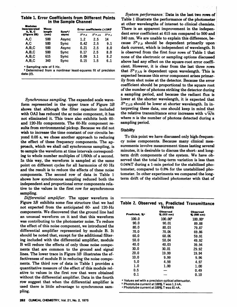
Table 2. Observed

Predicted, %#{176}

100.090.080.070.060.050.040.030.020.010.05.01.00.50.1

vs. PredictedValues

Observed

% (615 nm)

100. OOb90.0180.0370.0660.0650.0440.0330.0119.999.994.981.00

Transmittance

Observed%(500nm)

100. 0089.8879.8769.8659.9149.9239.9429.9219.949.964.971.000.490.10

#{176}Values set with a precision optical attenuator.b Phototube current at 100% 1 was 1.3 nA.

Phototu be current at 100% T was 81 nA.

252 CLINICAL CHEMISTRY, Vol. 21, No.2, 1975

Table 1. Error Coefficients from Different Pointsin the Sample Channel

Modul.sIncorporated Wave-

A, B, C length(Figure 2B) (nm)

Sync4/async

Error coefficients (X1091

S#{176}r.o Sr.i

A,C 500 Async 1.2 2.5 14A,C 500 Sync 0.42 2.5 9.1A,B,C 500 Async 0.21 2.5 8.0A,B,C 500 Sync 0.17 2.5 8.0AIB,C 615 Sync 0.09 3.1 8.2A,B,C 340 Sync 0.15 1.5 6.1

#{176}Sampling rate of 5 Hz.Determined from a nonllnear least.squares fit of precision

data (3).

Synchronous sampling. The expanded scale wave-form represented in the upper trace of Figure 3Bshows that although the filter capacitor includedwith 0A2 has reduced the ac noise component, it hasnot eliminated it. This trace also exhibits both 60-and 120-Hz components. The 60-Hz component re-sults from environmental pickup. Because we did notwish to increase the time constant of our circuits be-yond 0.05 s, we chose another approach to reducingthe effect of these frequency components. The ap-proach, which we shall call synchronous sampling, isto sample the waveform at time intervals correspond-ing to whole number multiples of 1/60th of a second.In this way, the waveform is sampled at the samepoint on different cycles for all harmonics of 60 Hzand the result is to reduce the effects of these noisecomponents. The second row of data in Table 1shows how synchronous sampling reduced both theindependent and proportional error components rela-tive to the values in the first row for asynchronoussampling.

Differential amplifier. The upper waveform inFigure 3B exhibits some fine structure that we hadnot expected from the anticipated 60- and 120-Hzcomponents. We discovered that the ground line hadan unusual waveform on it and that this waveformwas contributing to the photometer noise. To reducethe effect of this noise component, we introduced thedifferential amplifier represented by module B. Itshould be noted that, except for the additional filter-ing included with the differential amplifier, moduleB will reduce the effects of only those noise compo-nents that are common to the ground and signallines. The lower trace in Figure 313 illustrates the ef-fectiveness of module B in reducing the noise compo-nents. The third row of data in Table 1 provides aquantitative measure of the effect of this module rel-ative to values in the first row that were obtainedwithout the differential amplifier. Data in the fourthrbw suggest that when the differential amplifier isused there is little advantage to synchronous sam-pling.

System performance: Data in the last two rows ofTable 1 illustrate the performance of the photometerat other wavelengths of interest to clinical chemists.There is an apparent improvement in the indepen-dent error coefficient at 615 nm compared to 500 and340 nm. We are unable to explain this difference, be-cause S#{176}T,oshould be dependent primarily upondark current, which is independent of wavelength. Itis observed from the first four rows of Table 1 thatnone of the electronic or sampling options discussedabove had any effect on the square-root error coeffi-cient. However, it is clear from the last three rowsthat S#{176}T,1/2is dependent upon wavelength. This isexpected because this error component arises primar-ily from shot noise at the detector. Because the errorcoefficient should be proportional to the square rootof the number of photons striking the detector duringa sampling period, and because the radiant flux islower at the shorter wavelength, it is expected thatS#{176}T,1/2should be lower at shorter wavelength. In in-terpreting these data, one should keep in mind thatthe relative transmittance error increases with v’ii7nwhere n is the number of photons detected during asampling period.

Stability

To this point we have discussed only high-frequen-cy noise components. Because many clinical mea-surements involve measurement times lasting severalminutes, it is desirable to discuss the short- and long-term drift components of the system. We have ob-served that the total long-term variation is less than0.04%T during a 1-mm period for the stabilized pho-tometer, compared to 0.8% for the unstabilized pho-tometer. In other experiments we compared the long-term drift of the stabilized photometer with that of

l5

10.0

ISLO

//

/

1.0 2.0

Table 3. Predicted and Observed Precision for Kin;tic AnalysesInitial relative SD, %

No. analyses (nm) species error X 10’ (S#{176}r,oX 109 interval X 10’ Abs. Pred.#{176} Obs.

7 615 Chol. 0.55 1.5 3.5 2.06 3.6 3.9

12 615 Chol. 4.5 4.6 4.5 098 1.3 2.120 615 Chol. 56 56 5.0 0.00 Li 1.1

7 340 LDH 5.6 5.8 12 1.00 0.5 1.17 340 LDH 5.6 5.8 24 1.00 0.3 3.67 340 SGOT 5.6 5.8 8.5 0.80 0.6 1.87 340 SCOT 5.6 5.8 25 0.80 0.2 1.0

#{176}Predicted values (eq. 13c, ref. 3); S#{176}’,,= 8.2 >< 10’, S#{176}.,i,= 3.1 X 10’.Values calculated from Q= T/(/12 X 1023) ref. 3

#{176}Independent error calculated from S#{176}T,o= v’(quantitation error)’ + (dark current)’; dark current = 1.5 X 10’.

CLINICAL CHEMISTRY, Vol. 21, No. 2, 1975 253

the same lamp powered by an ac source regulated to

0.1%. During 30 mm the stabilized photometer drift-ed less than 0.03%T, while the ac-powered photome-ter drifted by about 0.4%T.

Linearity

Cannon and Butterworth (8) have pointed out thatconformance to Beer’s law does not necessarily en-sure that photometer response is linear. Therefore weused a linear transmittance system (Model 2001;Technometrics Inc., Purdue Research Park, Lafay-ette, md. 47906) to evaluate the linearity of the stabi-lized photometer. Data in Table 2 illustrate theagreement between expected and observed transmit-tancps for two wavelengths. Regression equations forpredicted vs. observed transmittances at 500 and 615nm are y = 0.999 (±0.001) x - 0.028 and y = 1.000(±0.001) x - 0.001, respectively. The uncertainty ex-pected from the linear transmittance system was lessthan 0.001 T. Taken as a group, the data in Table 2represent a linear dynamic range of phototube cur-rents over four orders of magnitude. This observationis supported by the fact that the root mean squarevalues of the error coefficients in the last four rows ofTable 1 are all less than 1 X 10’T or 0.01% T.

Evaluation for Kinetic Analyses

Because data presented to this point have beenbased solely on experiments designed to simulatechemical measurements, it is desirable to determinehow well these data represent the situation for chem-ical analyses. Recognizing that concentration errorsfor kinetic methods based on measurements of smallabsorbance intervals, z.A, are very sensitive to smallphotometric errors and to the absorbance at whichthe measurement is made (see ref. 3 and dashedcurve in Figure 4), we elected to use kinetic analysesto evaluate the validity of data reported above.Chemical systems chosen for this study included ki-netic methods for cholesterol (9), lactate dehydroge-nase (EC 1.1.1.27), and aspartate aminotransferase(EC 2.6.1.1). The cholesterol system was selected be-

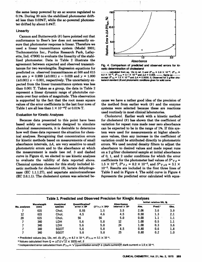
AbsorbonceFig. 4. Comparison of predicted and observed errors for ki-netic determination of cholesterol

, calculated from eq. 13c In ret. 3 and S#{176}= 5.6 X 1O, S#{176}7.,=

8.2 X iO, S#{176}T.1/2= 3.1 X 10 and A = 0.005.-, Same asexcept S#{176}r,o= 1.5 X 106 and &A = 0.0035.0. Observed foi 2 9/liter cho-lesterol standard ( and photometric condItions given for solid curve

cause we have a rather good idea of the precision ofthe method from earlier work (9) and the enzymesystems were selected because these are reactionsused routinely in most clinical laboratories.

Cholesterol. Earlier work with a kinetic methodfor cholesterol (9) has shown that the coefficient ofvariation for repeat runs made near zero absorbancecan be expected to be in the range of 1%. If this sys-tem were used for measurements at higher absorb-ance values, then any increase in the coefficient ofvariation could be attributed directly to photometricerrors. We used neutral density filters to adjust theabsorbance to desired values and made repeat runson a 2 g/liter cholesterol sample at initial absorbanceof 0, 1, and 2 under conditions for which the errorcoefficients for the photometer had values of S#{176}T,o=

1.5 X 106, S#{176}T,1= 8.2 X 10, and S#{176}T,1/2= 3.1 X10’. Results are included in the first three lines ofTable 3 and in Figure 4. The solid curve in Figure 4tepresents the predicted error calculated with equa-

254 CLINICAL CHEMISTRY, Vol. 21. No. 2, 1975

tion i3c from ref. 3, the error coefficients givenabove, and an absorbance interval of #{163}4= 0.0035.The open circles represent experimental values forcholesterol measured with initial absorbances of 0, 1,and 2, and #{163}4= 0.0035. While agreement betweenthe predicted curve and experimental results is notexact, we believe the agreement is sufficiently closeto confirm the general validity of our procedures andthe data presented above.

Enzymes. Commercial reagent preparations were

used for lactate dehydrogenase and aspartate amino-transferase in reconstituted sera. The last four rowsof data in Table 3 summarize conditions and resultsfor two groups of analyses for each enzyme. Theagreement between predicted and observed precisionis not as good as in the case of cholesterol. We believethat a major reason for the differences is the ob-served nonlinearity of absorbance vs. time plots. Thisposition is supported by the fact that comparableprecision is achieved for cholesterol with smaller ab-sorbance intervals.

We believe this report demonstrates that our treat-ment of photometric errors can be a useful guide inthe design and evaluation of photometric instrumen-tation and that the optical feedback photometer isuseful for precise measurements of small absorbanceintervals.

This investigation was supported in part by Grant No. GM13326-08 from the NIH, USPHS. We are grateful to Mr. WilliamOsgood of Biodynamics, Indianapolis, md. 46250 for supplying uswith their UV enzymatic SGOT kit for evaluation.

References

1. Proposed establishment of product class standard for detectionor measurement of glucose. Fed. Regist., 39 (126), Part III, June28(1974).

2. Bowers, G. N., Jr., Analytical problems in biomedical researchand clinical chemistry. In Analytical Chemistry: Key to Progress inNational Problems, Nat. Bur. Stand. Spec. Pubi. No. 351, Supt. ofDocuments, Govt. Printing Office, Washington, D. C. 20402, 1972,pp 77-157.3. Pardue, H. L., Hewitt, T. E., and Milano, M. J., Photometric er-

,,-rors in equilibrium and kinetic analyses based upon absorptionspectroscopy. Clin. Chem. 20, 1028(1974).

4. Pardue, H. L., and Rodriquez, P. A., High-stability photometerutilizing optical feedback. Anal. Chem. 39,901 (1967).

5. Pardue, H. L., and Deming, S. N., High-stability low-noise pre-cision spectrometer using optical feedback. Anal. Chem. 41, 986(1969).

6. Pardue, H. L., and Miller, M. M., Multichannel analyzer featur-ing ultrahigh stability photometry: Application to enzyme deter-mination. Clin. Chem. 18, 928 (1972).7. “RCA Solid State Databook Series SSD-206A.” RCA SolidState Division, Somerville, N. J., 1973, pp 398-403.8. Cannon, C. G., and Butterworth, I. S. C., Beer’s law and spec-trophotometer linearity. Anal. Chem. 25, 168 (1953).9. Hewitt, T. E., and Pardue, H. L., Kinetics of the cholesterol-sulfuric acid reaction: A fast kinetic method for serum cholesteroLClin. Chem. 19, 1128 (1973).