theory of profit economic policy mbs first year

8/8/2019 Theory of Profit Economic Policy MBS First Year

http://slidepdf.com/reader/full/theory-of-profit-economic-policy-mbs-first-year 1/18



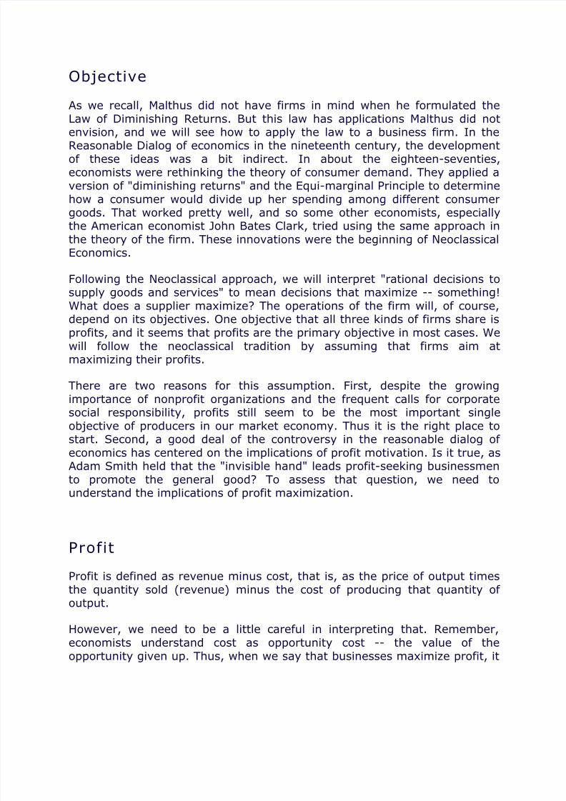
is important to include all costs - whether they are expressed in moneyterms or not.

For example, a cab-driver - the self-employed proprietor of an independentcab service - says: "I'm making a 'profit,' but I can't take home enough to

support my family, so I'm going to have to close down and get a job." Theproprietor is ignoring the opportunity cost of her own labor. When thoseopportunity costs are taken into account, we will find that he is not reallymaking a profit after all.

Let's say that the cab-driver makes $500 a week driving his cab, after allexpenses (gasoline, maintenance, etc.) have been taken out. Suppose hecan get wages (including tips!) of $800 driving for someone else, with hoursno longer and about the same conditions otherwise. Then $800 is theopportunity cost of his labor, and after we deduct the opportunity cost fromhis $500 net as an independent cabbie, he is actually losing $300 per week.

This is one of the most important reasons for using the opportunity costconcept: it helps us to understand the circumstances that will lead people toget into and out of business.

Because accountants traditionally considered only money costs, the net of money revenue minus money cost is called "accounting profit." (Actually,modern accountants are well aware of opportunity cost and use the conceptfor special purposes). The economist's concept is sometimes called"economic profit." If there will be some doubt as to which concept of profit

we mean, we will sometimes use the terms "economic profit" or "accountingprofit" to make it clear which is intended.

The John Bates Clark Model

Like any other unit, a firm is limited by the technology available. Thus, it canincrease its outputs only by increasing its inputs. As usual, this will beexpressed by a production function. The output the firm can produce will

depend on the land, labor and capital the firm puts to work.

In formulating the neoclassical theory of the firm, John Bates Clark took overthe classical categories of land, labor and capital and simplified them in twoways. First, he assumed that all labor is homogenous - one labor hour is aperfect substitute for any other labor hour. Second, he ignored thedistinction between land and capital, grouping together both kinds of



nonhuman inputs under the general term "capital." And he assumed thatthis broadened "capital" is homogenous.

Of course, the simplifying assumptions aren't true - John Bates' Clark'sconception of the firm is highly simplified, like a map at a very large scale.

In more advanced economics, we can get rid of the simplifying assumptionsand deal with a much more realistic "map" of the business firm. But for mostof this book, we'll take that on faith, and stick to the simplified version Clarkgave us. That will make it simpler, and the principles we will discover aresound and applicable to the real world in all its complexity.

In the John Bates Clark model, there are some important differencesbetween labor and capital, and they relate to the long and short run.

Short and Long Run

A key distinction here is between the short and long run.

Some inputs can be varied flexibly in a relatively short period of time. Weconventionally think of labor and raw materials as "variable inputs" in thissense. Other inputs require a commitment over a longer period of time.Capital goods are thought of as "fixed inputs" in this sense. A capital goodrepresents a relatively large expenditure at a particular time, with theexpectation that the investment will be repaid -- and any profit paid -- by

producing goods and services for sale over the useful life of the capital good.In this sense, a capital investment is a long-term commitment. So capital isthought of as being variable only in the long run, but fixed in the short run.

Thus, we distinguish between the short run and the long run as follows:

In the perspective of the short run, the number and equipment of firmsoperating in each industry is fixed.

In the perspective of the long run, all inputs are variable and firms can come

into existence or cease to exist, so the number of firms is also variable.

More Simplifying Assumptions

The John Bates Clark model of the firm is already pretty simple. We arethinking of a business that just uses two inputs, homogenous labor and



homogenous capital, and produces a single homogenous kind of output. Theoutput could be a product or service, but in any case it is measured inphysical (not money) units such as bushels of wheat, tons of steel orminutes of local telephone calls. In the short run, in addition, the capitalinput is treated as a given "fixed input." Also, we can identify the price of

labor with the wage in the John Bates Clark model. (In a modern businessfirm, we have to include benefits as well as take-home wages. The technicalterm for the total, wages and benefits, is "employee compensation.")

We will add two more simplifying assumptions. The new simplifyingassumptions are:

• The price of output is a given constant.

• The wage (the price of labor per labor hour) is a given constant.

Putting them all together -- just two kinds of input and one kind of output,one kind of output fixed in the short run, and given output price and wage --it seems to be a lot of simplifying assumptions, and it is. But, as we will seein later chapters of the book, these are not arbitrary simplifyingassumptions. They are the assumptions that fit best into many applications,and the starting point for still others.

Once we have simplified our conception of the firm to this extent, what isleft for the director of the firm to decide?

The Firm’s Decision

In the short run, then, there are only two things that are not given in theJohn Bates Clark model of the firm. They are the output produced and thelabor (variable) input. And that is not actually two decisions, but just one,since labor input and output are linked by the "production function." Either

• The output is decided, and the labor input will have to be just enoughto produce that output

or• The labor input is decided, and the output is whatever that quantity of

labor can produce.

Thus, the firm's objective is to choose the labor input and correspondingoutput that will maximize profit.



Let's continue with the numerical example in the first part of the chapter.Suppose a firm is producing with the production function shown there, in theshort run. Suppose also that the price of the output is $100 and the wageper labor-week is $500. Then let's see how much labor the firm would use,and how much output it would produce, in order to maximize profits.

The relationship between labor input and profits will look something like this:

Figure: Labor Input and Profits in the Numerical Example

In the figure, the green curve shows the profits rising and then falling andthe labor input increases. Of course, the eventual fall-off of profits is a resultof "diminishing returns," and the problem the firm faces is to balance"diminishing returns" against the demand for the product. The objective is toget to the top of the profit hill. We can see that this means hiring somethingin the range of four to five hundred workers for the week. But just howmany?

The way to approach this problem is to take a bug's-eye view. Think of yourself as a bug climbing up that profit hill. How will you know when youare at the top?

The Marginal Approach

The bug's-eye view is the marginal approach. However much labor is beingemployed at any given time, the really relevant question is, supposing onemore unit of labor is hired, will profits be increased or decreased? If one unitof labor is eliminated, will profits increase or decrease? In other words, what



does one additional labor unit adds to profits? What would elimination of onelabor unit subtract from profits?

We can break that question down. Profit is the difference of revenue minuscost. Ask, "What does one additional labor unit add to cost? What does one

additional labor unit add to revenue?

The first question is relatively easy. What one additional labor unit will addto cost is the wage paid to recruit the one additional unit.

The second question is a little trickier. It's easier to answer a relatedquestion: "What does one additional labor unit add to production?" Bydefinition, that's the marginal product -- the marginal product of labor isdefined as the additional output as a result of increasing the labor input byone unit. But we need a measurement that is comparable with revenues andprofits, that is, a measurement in money terms. Since the price is given, themeasurement we need is the Value of the Marginal Product:

Value of the Marginal Product The Value of the Marginal Product is the product of the marginalproduct times the price of output. It is abbreviated VMP.

To review, we have made some progress toward answering the originalquestion. Adding one more unit to the labor input, we have

increase in revenue = value of marginal product

increase in cost = wage

So the answer to "What will one additional labor unit add to profits?" is "thedifference of the Value of the Marginal Product Minus the wage." Conversely,the answer to "What will the elimination of one labor unit add to profits?" is"the wage minus the Value of Marginal Product of Labor." And in either casethe "addition to profits" may be a negative number: either building up thework force or cutting it down can drag down profits rather than increasingthem.

So, again taking the bug's-eye view, we ask "Is the Value of the MarginalProduct greater than the wage, or less?" If greater, we increase the laborinput, knowing that by doing so we increase profits by the difference, VMP-wage. If less, we cut the labor input, knowing that by doing so we increaseprofits by the difference, wage-VMP. And we continue doing this until theanswer is "Neither." Then we know there is no further scope to increaseprofits by changing the labor input -- we have arrived at maximum profits.



Let's see how that works. Let's go back to the numerical example from earlier in the chapter, and assume that the price of output is $100 per unit and the

wage is $500. In Figure 8, below, we have the value of the marginal

product, $100*MP, and the wage for that example.

Now suppose that the firm begins by using just 200 units of labor, as shownby the orange line. The manager asks herself, "If I were to increase thelabor input to 201, which would increase both costs and revenues. By howmuch? Let's see: the VMP is 850, so the additional worker will add $850 torevenues. Since the wage is $500, the additional worker will add just $500to cost, for a net gain of $350. It's a good idea to "upsize" and adds one

more worker.

On the other hand, suppose that the firm is using 800 units of labor, asshown by the other orange line. The manager asks herself, "If I were to cutthe labor input to 799, which would cut both costs and revenues. By howmuch? Let's see: the VMP is 200, so the additional worker will add just $200to revenues. Since the wage is $500, the additional worker will add just$500 to cost, for a net loss of $300. It's time to "downsize" and cut the laborforce.

In each case, there is an unrealized potential, and the amount of unrealized

potential is the difference between the VMP and the wage. The firm's profitpotential will not be 100% realized until the VMP is equal to the wage. That'sthe "equi-marginal principle" again.



The Equi-marginal Principle

By taking the marginal approach -- the bug's-eye view -- we havediscovered the diagnostic rule for maximum profits. The way to maximizeprofits then is to hire enough labor so that

VMP=wage

Where, p is the price of output and VMP = p*MP the marginal productivity of labor in money terms.

This is another instance of the Equi-marginal Principle. The rule tells us thatprofits are not maximized until we have adjusted the labor input so that themarginal product in labor, in dollar terms, is equal to the wage. Since thewage is the amount that the additional (marginal) unit of labor adds to cost,

we could think of the wage as the "marginal cost" of labor and express therule as "value of marginal product of labor equal to marginal cost." But wewill give a more compete and careful definition of marginal cost (of output)in the next chapter.

Profit Maximization Example

Here is an instance that shows the maximization of profits in the example.Remember, the wage is $500 per labor week. The theory tells us that profitswill be biggest when the value of the marginal product is exactly equal to thewage, that is, $500. Try adjusting the number of labor weeks input and seehow profits increase as the value of the marginal product gets closer to$500.

Program Example 3

Click here to see the result:

Labor Input Marginal

PhysicalProduct

Value of

MarginalProduct

Wage Profit

100 8.9 890 500 44500

Again, if you read JavaScript, take a look at the source of the page to seethe mathematical background of this example.



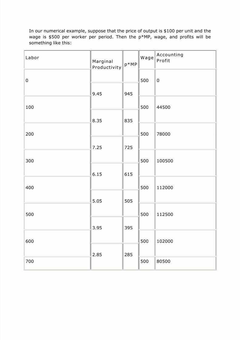
In our numerical example, suppose that the price of output is $100 per unit and the

wage is $500 per worker per period. Then the p*MP, wage, and profits will be

something like this:

Labor Marginal

Productivityp*MP

Wage

Accounting

Profit

0 500 0

9.45 945

100 500 44500

8.35 835

200 500 78000

7.25 725

300 500 100500

6.15 615

400 500 112000

5.05 505

500 500 112500

3.95 395

600 500 102000

2.85 285

700 500 80500



1.75 175

800 500 48000

0.65 65

900 500 4500

-0.45 -55

1000 500 -50000

Visualizing P rofit Maximization

What we see in the table is that the transition from 400 to 500 units of laborgives p*MP=505, very nearly VMP=wage. And that is the highest profit. Sothe profit-maximizing labor force is about 500 units.

We can get a more exact answer by looking at a picture or tinkering with theprogram example a bit. Here is a picture of the profit-maximizing hiring in

this example:

Figure 9: Maximizing Profit

The picture suggests that the exact amount is a bit less than 500 units of labor. If you tinker with the program example enough, you will see that the



Increasing Returns to scale and long run

In microeconomics, we think of diminishing returns as a short run thing. Inthe long run, all inputs can be increased or decreased in proportion.Reductions in the marginal productivity of labor, due to increasing the labor

input, can be offset by increasing the tools and equipment the workers haveto work with. How will that come out, on net? The answer is -- "it alldepends!"

In the long run we define three possible cases:

Decreasing returns to scale If an increase in all inputs in the same proportion k leads to anincrease of output of a proportion less than k, we have decreasingreturns to scale. Example: If we increase the inputs to a dairy farm

(cows, land, barns, feed, labor, everything) by 50% and milk outputincreases by only 40%, we have decreasing returns to scale in dairyfarming. This is also known as "diseconomies of scale," sinceproduction is less cheap when the scale is larger.

Constant returns to scale If an increase in all inputs in the same proportion k leads to anincrease of output in the same proportion k, we have constant returnsto scale. Example: If we increase the number of machinists andmachine tools each by 50%, and the number of standard piecesproduced increases also by 50%, then we have constant returns inmachinery production.

Increasing returns to scale If an increase in all inputs in the same proportion k leads to anincrease of output of a proportion greater than k, we have increasingreturns to scale. Example: If we increase the inputs to a softwareengineering firm by 50% output and increases by 60%, we haveincreasing returns to scale in software engineering. (This might occurbecause in the larger work force, some programmers can concentratemore on particular kinds of programming, and get better at them).This is also known as "economies of scale," since production is cheaperwhen the scale is larger.

In introductory economics, we usually discuss these long run tendencies inthe context of cost analysis, rather than marginal productivity analysis.However, increasing returns to scale, in particular, creates somecomplications for the application of marginal productivity thinking. Thus, Ithink there may be something to gain by exploring how increasing returns toscale goes together with marginal productivity. To keep it as simple aspossible, we will look at a numerical example of a two-person labor market



and a fictitious product that is produced with increasing returns to scale.Economists often like to talk about the production of "widgets," so ourfictitious industry is the widget-tying industry.

Examples of Production with increasing returns to scale

• Since this is a long run analysis, there is no fixed input. Indeed, forsimplicity, there is only one input. Labor is the only input and isvariable.

• Our small economy is populated by three people: Bob and John,workers, and Gordon, an entrepreneur (that is, a person who willorganize a business if and only if it is profitable to do so).

• o Bob, working alone, can produce output worth 2000 per week.o Bob's opportunity cost is 2100 per week. (That means Bob can

earn 2100 in producing some other good or service).• o John, working alone, can produce 2000 per week.

o John's opportunity cost is 2800 per week.• If Bob and John work together, thanks to division of labor, they can

produce 5500 per week. Suppose, for example, that Gordon sets up aWidget-Tying business and hires Bob and, later, John to do the work.This is an example of "increasing returns to scale" since inputincreases by 100% when the second worker is hired and output

increases by 175% as a result.

Why would output increase more than in proportion to inputs? First, simplyhaving four hands may increase productivity as the two men cansimultaneously do different parts of the job. Second, each may concentrateon some part of the work, getting better at it with more practice, but leavingthe other part to the other worker who also gains practice and skill in thatpart. (These were the kinds of advantages Adam Smith particularlystressed). Finally, each may concentrate on the tasks for which he has agreater inborn talent.

Notice that the two-person widget-tying operation uses resources with anopportunity cost of 2800+2100=4900 and produces output worth 5500, fora net increase in production of 600. Evidently, it is a good thing that such ateam be organized.



Marginal Productivity and Increasing Returns toScale

Now, what is the marginal productivity of labor with two persons employed?With one worker, output was 2000; with two, 5500, for a difference of 3500.If either Bob or John quits, reducing the firm to 1 worker, the firm loses3500 -- so 3500 is the marginal productivity of both Bob and John. That is,3500 is the marginal productivity of labor, between 1 and 2 units of labor,not the marginal product of some specific worker who happens last. Here isthe marginal productivity of labor in the form of a table. Remember, the lawof diminishing marginal productivity does not apply in this long runperspective, since there is no fixed input.

Labor Output MP

0 0

1 2000 2000

2 5500 3500

But see what this means. If both Bob and John are paid their marginalproductivity, the wage bill is 2*3500=7000. But the product of the firm isonly 5500, so Gordon ends up losing 1500.

Clearly, it will not be possible to pay the marginal productivity wage.Suppose both are paid a wage less than marginal productivity. Will theycontinue to work for Gordon if they are paid less than marginal productivity?Yes, up to a point. Here is the supply curve of labor derived from theiropportunity costs:



The Supply of Labor from Bob and John

How much does Gordon have to pay? Suppose Gordon starts cutting thewage. When the wage drops below 2800, John will resign, and then the firmproduces only 2000, not enough to pay Bob his 2100 opportunity cost, so

Bob resigns too. Evidently 2800 is the least wage Gordon can pay and keephis work force. However, at a wage of 2800 per worker, Gordon's wage bill is5600, and with an output of 5500, he is still losing 100. Not as much asbefore, but a loss is a loss, and Gordon will choose not to set up a widget-tying enterprise.

The Dark Side of Force

Increasing returns to scale are a powerful force for increasing productivity,but the problem of organizing them efficiently is "the dark side of the force."We have seen that an enterprise that yields a net gain of 600 to societycannot be organized, in this example, without producing a loss. The marketsystem cannot take advantage of the potentiality for gain through division of labor and increasing returns to scale in this case. This possibility wasdiscovered by an early 20th Century British economist named Arthur CharlesPigou, but despite 80 years of discussion, this analysis is not at all widelyunderstood, even among professional economists. Pigou thought it might bea good idea for the government to subsidize enterprises with increasing

returns to scale. In this case a subsidy of 150 would make the widget-tyingenterprise profitable and produce a gain of 600 in national product.

There may be another solution. Since the widget-tying enterprise adds 600to national output but loses at least 100, we might ask, what happens to thedifference of 700? The answer is that Bob gets it. Bob is paid at least 2800but his opportunity cost is only 2100, accounting for the difference of 700.Suppose that Bob and John were not paid the same wage, but, instead, eachwas paid his opportunity cost plus 100. The wage bill would then be2200+3000=5200 and Gordon would finish with a profit of 300. Thus, wagediscrimination may make it possible for the widget-tying enterprise to exist

when it cannot exist so long as each worker is paid the same wage for thesame work.

The conclusions are surprising, and understandably, controversial -- yet thenumbers support them, both in this and more complicated and abstractexamples.



1. Some people believe it is just that each person be paid according toher or his contribution, and interpret "marginal productivity" as theperson's contribution. However, this may impossible when there areincreasing returns to scale, as there may not be enough output to payeveryone on that basis.

2. Compromising, some would say that each person ought to be paid inproportion to her or his contribution, so that people are paid equallyfor the same work. That, too, may be impossible.

3. Discrimination or subsidy may be necessary to allow some sociallyuseful activities to exist.

4. There may be no simple system of payment (such as supply anddemand or equal pay for equal work) that will allow a socially usefulenterprise with increasing returns to scale to exist.

Reflections

I think this is the reason we have organizations. If there were no increasingreturns to scale, there would be little reason for any business to employmore than one person. We would instead have an economy consisting of self-employed individuals, like a yeoman agricultural system. Instead we seean economic system consisting in part of large, complicated organizationswith internal arrangements and payments systems that have little to do withcontributions or marginal productivity, and may be discriminatory. From anabstract point of view, they may waste resources by not paying at the

marginal productivity; but the benefits of increasing returns to scale are sogreat that, even falling far short of potential efficiency, they can still be veryproductive.

This is sometimes lost sight of by the organizations themselves. Peoplenaturally avoid complexity, and organizations sometimes try to set upsimple, market-like internal payment and fund transfer systems, hoping thatthis will increase efficiency. But, as we have seen, this can fail badly in thecontext of increasing returns to scale (and that is the context of any largeproductive organization). We have recently been through such an experience

at Drexel. A few years ago we went over to "revenue centered budgeting."The idea was to let the colleges retain a high proportion of the revenues theyproduce, through tuition, grants, and contracts and so on. This would (it wasfelt) give the deans and college faculties more "incentive" to set up popularnew programs and initiatives. However, it wasn't possible to let the collegeskeep 100%, since some money is needed to run shared services like thecomputer center, student-life activities, and the library, not to mention thesalaries of high administrators (and we wouldn't think of mentioning that).



But it couldn't be made to work. If the proportion kept by the colleges washigh enough to make it profitable for them to set up new programs andinitiatives, there was not enough for the purposes of the centraladministration; while if the proportion taken by the central administrationwas enough to do its job, then the colleges were losing money on their new

programs and initiatives -- no incentive! So Drexel has moved away from"revenue centered budgeting" in practice, although there is still some workbeing done to try to work out a "revenue centered budgeting" system thatwill work. Here's a prediction based on the theory of increasing returns toscale: a revenue-centered budgeting system probably can be made to work,but it will be just as complex and frustrating than the centralized budgetingtraditionally has been. That complexity and frustration (and largeorganizations) are the price we pay for the benefits of increasing returns toscale.

Summary

We have seen that the concept of marginal productivity and the law of diminishing marginal productivity play central parts in both the efficientallocation of resources in general and in profit maximization in the JohnBates Clark model of the business firm.

The John Bates Clark model and the principle of diminishing marginalproductivity provide a good start on a theory of the firm and of supply. In

applying the marginal approach and the equi-marginal principle to profitmaximization, it extends our understanding of the principles of efficientresource allocation. Some key points in the discussion have been

• the distinction between marginal productivity and average productivity• the "law of diminishing marginal productivity"

• the rule for division of a resource between two units producing thesame product: equal marginal productivities

• the diagnostic formula VMP=wage, that tells us the input and outputare adjusted to maximize profits in the business firm, in the short run

• In the long run, there may be increasing, decreasing, or constantreturns to scale. Increasing returns to scale will complicate thingssomewhat for the marginal productivity approach.

This has given us a start on the theory of the business firm. But we will wantto reinterpret the model of the firm in terms of cost -- since the coststructure of the firm is important in itself, and important for anunderstanding of supply.



Why wealth maximization is considered to be

better operating goal than Profit maximization?

Frequently, maximization of profits is regarded as the proper objective of the

firm, but it is not as inclusive a goal as that of maximizing stockholderwealth. For one thing, total profits are not as important as earnings perstock. A firm could always raise total profits by issuing stock and using theproceeds to invest in Treasury bills. Even maximization of earnings perstock, however, is not a fully appropriate objective, partly because it doesnot specify the timing or duration of expected returns. Is the investmentproject that will produce a $100,000 return 5 years from now more valuablethan the project that will produce annual returns of $15,000 in each of thenext 5 years? An answer to this question depends upon the time value of money. Few existing stockholders would think favorably of a project that

promised its first return in 100 years, no matter how large this return. Wemust take into account the time pattern of returns in our analysis.

Another shortcoming of the objective of maximizing earnings per stock isthat it does not consider the risk or uncertainty of the prospective earningsstream. Some investment projects are far more risky than others. As aresult, the prospective stream of earnings per stock would be moreuncertain if these projects were undertaken. In addition, a company will bemore or less risky depending upon the amount of debt in relation to equity inits capital structure. This financial risk is another uncertainty in the minds of investors when they judge the firm in the marketplace. Finally, an earnings

per stock objective does not take into account any dividend the companymight pay.

For the reasons given, an objective of maximizing earnings per stock maynot be the same as maximizing market price per stock. The market price of a firm's stock represents the value that market participants place on the firm

theory of profit economic policy mbs first year

Documents