theory of distributed computing i - inet
TRANSCRIPT
Theory ofDistributed Computing I
Algorithms and Lower Bounds
(Part 2: Message Passing)
Dr. Stefan SchmidCo-lecturer (shared memory): Dr. Petr Kuznetsov
Thanks to Prof. Dr. Roger Wattenhofer for basis of manuscript!
Spring 2011
Introduction
In the second part of this course, we turn our attention to distributed computingin networks, i.e., where computers (or processors) communicate via messagepassing along the links of the communication network. Typical “old school”examples are parallel computers, or the Internet whose architecture often followsthe design principle of decentralization to avoid bottlenecks and single pointsof failures. More recent application examples of distributed systems includepeer-to-peer systems, sensor networks, and multi-core architectures.
These applications have in common that, like in the first part of the course,many processors or entities (often called nodes) are active in the system at anymoment. The nodes have certain degrees of freedom: they may have their ownhardware, their own code, and sometimes their own independent task. Never-theless, the nodes may share common resources and information, and, in order tosolve a problem that concerns several—or maybe even all—nodes, coordinationis necessary. Despite these commonalities, a peer-to-peer system, for example,is quite different from a multi-core architecture. In some systems the nodes op-erate synchronously, in other systems they operate asynchronously. There aresimple homogeneous systems, and heterogeneous systems where different typesof nodes, potentially with different capabilities, objectives etc., need to interact.There are different communication techniques. Sometimes the communicationinfrastructure is tailor-made for an application, sometimes one has to work withany given infrastructure. The nodes in a system sometimes work together tosolve a global task, occasionally the nodes are autonomous agents that havetheir own agenda and compete for common resources.
This second part of the course continues to study basic principles of distrib-uted computing. In particular, we are interested in the following challenges indistributed systems with message passing:
1. Network Design: What is a “good” communication network for messagepassing?
2. Communication: What is the cost of communication? (Often commu-nication cost dominates the cost of local processing or storage. Sometimeswe may even assume that everything but communication is free!)
3. Locality/Scalability: Networks keep growing. Luckily, global informa-tion is not always needed to solve a task, often it is sufficient if nodes talkto their neighbors. We will address the fundamental question in distrib-uted computing whether a local solution is possible for a wide range ofproblems.
1

2
Unfortunately, a complete coverage of this active and exciting field is impos-sible, and we focus on highlighting common themes and techniques. We will setoff with some evergreen problems such as Leader Election that give a feelingfor the main setting and the tradeoffs. We will also study classic problems fromtheoretical computer science, such as Maximal Independent Set, from thenew perspective of distributed computing. A highlight of the course might bethe Vertex Coloring algorithms: vertex coloring is the problem of how toassign colors to nodes in a network, such that no two adjacent nodes have thesame color. Colorings are for example important in wireless networks: nodeswhich are close to each other should use different frequency bands (i.e., colors)in order to avoid interference and minimize retransmissions. As we will see,the coloring problem and the independent set problem are closely related, andsolutions for one problem can be used for the other.
Finally, if time permits, we take a look at social networks. Interestingly,today we still do not know much about the structure and dynamics of thesenetworks, and research is very active in this field. Moreover, due to the niceproperties of these networks, researchers have proposed to build computer net-works similarly to social networks.
Have fun!

Chapter 1
Communication Networks
1.1 Example: Peer-to-Peer
The term peer-to-peer (P2P) is ambiguous and used in a variety of differentcontexts, such as:
• In popular media coverage, P2P is often synonymous to software or proto-cols that allow users to “share” files, often of dubious origin. In the earlydays, P2P users mostly shared music, pictures, and software; nowadaysbooks, movies or tv shows have caught on.
• In academia, the term P2P is used mostly in two ways. A narrow viewessentially defines P2P as the “theory behind file sharing protocols”. Inother words, how do Internet hosts need to be organized in order to delivera search engine to find (file sharing) content efficiently? A popular termis “distributed hash table” (DHT), a distributed data structure that im-plements such a content search engine. A DHT should support at least asearch (for a key) and an insert (key, object) operation. A DHT has manyapplications beyond file sharing, e.g., the Internet domain name system(DNS).
• A broader view generalizes P2P beyond file sharing: Indeed, there is agrowing number of applications operating outside the juridical gray area,e.g., P2P Internet telephony a la Skype, P2P mass player games on videoconsoles connected to the Internet, P2P live video streaming as in Zattooor StreamForge, or P2P social storage such as Wuala. So, again, what isP2P?! Still not an easy question... Trying to account for the new applica-tions beyond file sharing, one might define P2P as a large-scale distributedsystem that operates without a central server bottleneck. However, withthis definition almost everything we learn in this course is P2P! More-over, according to this definition early-day file sharing applications suchas Napster (1999) that essentially made the term P2P popular would notbe P2P! On the other hand, the plain old telephone system or the worldwide web do fit the P2P definition...
• From a different viewpoint, the term P2P may also be synonymous forprivacy protection, as various P2P systems such as Freenet allow publish-ers of information to remain anonymous and uncensored. (Studies show
3

4 CHAPTER 1. COMMUNICATION NETWORKS
that these freedom-of-speech P2P networks do not feature a lot of contentagainst oppressive governments; indeed the majority of text documentsseem to be about illicit drugs, not to speak about the type of content inaudio or video files.)
So we cannot hope for a single well-fitting definition of P2P, as some of themeven contradict. In the following we mostly employ the academic viewpoints(second and third definition above). In this context, it is generally believed thatP2P will have an influence on the future of the Internet. The P2P paradigmpromises to give better scalability, availability, reliability, fairness, incentives,privacy, and security, just about everything researchers expect from a futureInternet architecture. As such it is not surprising that new “clean slate” Internetarchitecture proposals often revolve around P2P concepts.
One might naively assume that for instance scalability is not an issue intoday’s Internet, as even most popular web pages are generally highly available.However, this is not really because of our well-designed Internet architecture,but rather due to the help of so-called overlay networks: The Google website forinstance manages to respond so reliably and quickly because Google maintains alarge distributed infrastructure, essentially a P2P system. Similarly companieslike Akamai sell “P2P functionality” to their customers to make today’s userexperience possible in the first place. Quite possibly today’s P2P applicationsare just testbeds for tomorrow’s Internet architecture.
1.2 P2P Architecture Variants
Several P2P architectures are known:
• Client/Server goes P2P: Even though Napster is known to the be first P2Psystem (1999), by today’s standards its architecture would not deserve thelabel P2P anymore. Napster clients accessed a central server that managedall the information of the shared files, i.e., which file was to be found onwhich client. Only the downloading process itself was between clients(“peers”) directly, hence peer-to-peer. In the early days of Napster theload of the server was relatively small, so the simple Napster architecturemade a lot of sense. Later on, it became clear that the server wouldeventually be a bottleneck, and more so an attractive target for an attack.Indeed, eventually a judge ruled the server to be shut down, in otherwords, he conducted a juridical denial of service attack.
• Unstructured P2P: The Gnutella protocol is the anti-thesis of Napster,as it is a fully decentralized system, with no single entity having a globalpicture. Instead each peer would connect to a random sample of otherpeers, constantly changing the neighbors of this virtual overlay networkby exchanging neighbors with neighbors of neighbors. (In such a systemit is part of the challenge to find a decentralized way to even discover afirst neighbor; this is known as the bootstrap problem. To solve it, usuallysome random peers of a list of well-known peers are contacted first.) Whensearching for a file, the request was being flooded in the network. Indeed,since users often turn off their client once they downloaded their contentthere usually is a lot of churn (peers joining and leaving at high rates) in

1.3. HYPERCUBIC NETWORKS 5
a P2P system, so selecting the right “random” neighbors is an interestingresearch problem by itself. However, unstructured P2P architectures suchas Gnutella have a major disadvantage, namely that each search will costm messages, m being the number of virtual edges in the architecture. Inother words, such an unstructured P2P architecture will not scale.
• Hybrid P2P: The synthesis of client/server architectures such as Napsterand unstructured architectures such as Gnutella are hybrid architectures.Some powerful peers are promoted to so-called superpeers (or, similarly,trackers). The set of superpeers may change over time, and taking downa fraction of superpeers will not harm the system. Search requests arehandled on the superpeer level, resulting in much less messages than inflat/homogeneous unstructured systems. Essentially the superpeers to-gether provide a more fault-tolerant version of the Napster server, allregular peers connect to a superpeer. As of today, many popular P2P sys-tems have such a hybrid architecture, carefully trading off reliability andefficiency, but essentially not using any fancy algorithms and techniques.
• Structured P2P: Inspired by the early success of Napster, the academicworld started to look into the question of efficient file sharing. Indeed, evenearlier, in 1997, Plaxton, Rajaraman, and Richa proposed a hypercubic ar-chitecture for P2P systems. This was a blueprint for many so-called struc-tured P2P architecture proposals, such as Chord, CAN, Pastry, Tapestry,Viceroy, Kademlia, Koorde, SkipGraph, SkipNet, etc. In practice struc-tured P2P architectures are not so popular yet, apart from the Kad (fromKademlia) architecture which comes for free with the eMule client, or thedistributed trackers used in BitTorrent (with millions of peers constitutingthe network which also resembles Kademlia). Indeed, also the Plaxton etal. paper was standing on the shoulders of giants. Some of its eminentprecursors are:
– Research on linear and consistent hashing, e.g., the paper “Consistenthashing and random trees: Distributed caching protocols for relievinghot spots on the World Wide Web” by Karger et al. (co-authoredalso by the late Daniel Lewin from Akamai), 1997.
– Research on locating shared objects, e.g., the papers “Sparse Parti-tions” or “Concurrent Online Tracking of Mobile Users” by Awerbuchand Peleg, 1990 and 1991.
– Work on so-called compact routing: The idea is to construct routingtables such that there is a trade-off between memory (size of routingtables) and stretch (quality of routes), e.g., “A trade-off betweenspace and efficiency for routing tables” by Peleg and Upfal, 1988.
– . . . and even earlier: hypercubic networks, see next section!
1.3 Hypercubic Networks
This section reviews some popular families of network topologies. These topolo-gies are used in countless application domains, e.g., in classic parallel computersor telecommunication networks, or more recently (as said above) in P2P com-puting. In the following, let us assume an all-to-all communication model, i.e.,

6 CHAPTER 1. COMMUNICATION NETWORKS
each node can set up direct communication links to arbitrary other nodes. Sucha virtual network is called an overlay network, or in this context, P2P architec-ture. In this section we present a few overlay topologies of general interest.
The most basic network topologies used in practice are trees, rings, grids ortori. Many other suggested networks are simply combinations or derivatives ofthese. The advantage of trees is that the routing is very easy: for every source-destination pair there is only one possible simple path. However, since the rootof a tree is usually a severe bottleneck, so-called fat trees have been used. Thesetrees have the property that every edge connecting a node v to its parent u hasa capacity that is equal to all leaves of the subtree routed at v. See Figure 1.1for an example.
2
1
4
Figure 1.1: The structure of a fat tree.
Remarks:
• Fat trees belong to a family of networks that require edges of non-uniformcapacity to be efficient. Easier to build are networks with edges of uniformcapacity. This is usually the case for grids and tori. Unless explicitlymentioned, we will henceforth treat all edges to be of capacity 1. In thefollowing, [x] means the set 0, . . . , x− 1.
Definition 1.1 (Torus, Mesh). Let m, d ∈ N. The (m, d)-mesh M(m, d) is agraph with node set V = [m]d and edge set
E =
(a1, . . . , ad), (b1, . . . , bd) | ai, bi ∈ [m],
d∑
i=1
|ai − bi| = 1
.
The (m, d)-torus T (m, d) is a graph that consists of an (m, d)-mesh and addi-tionally wrap-around edges from nodes (a1, . . . , ai−1,m, ai+1, . . . , ad) to nodes(a1, . . . , ai−1, 1, ai+1, . . . , ad) for all i ∈ 1, . . . , d and all aj ∈ [m] with j 6= i.In other words, we take the expression ai − bi in the sum modulo m prior tocomputing the absolute value. M(m, 1) is also called a line, T (m, 1) a cycle,and M(2, d) = T (2, d) a d-dimensional hypercube. Figure 1.2 presents a lineararray, a torus, and a hypercube.
1.3. HYPERCUBIC NETWORKS 7
011010
110
100
000 001
101
111
M(2,3)
0 1 2
M( ,1)m
−1m
01
02
00 10
11
12
03
20
21
22
13
30
31
32
23 33
(4,2)T
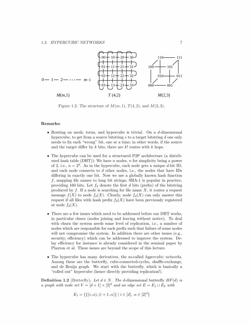
Figure 1.2: The structure of M(m, 1), T (4, 2), and M(2, 3).
Remarks:
• Routing on mesh, torus, and hypercube is trivial. On a d-dimensionalhypercube, to get from a source bitstring s to a target bitstring d one onlyneeds to fix each “wrong” bit, one at a time; in other words, if the sourceand the target differ by k bits, there are k! routes with k hops.
• The hypercube can be used for a structured P2P architecture (a distrib-uted hash table (DHT)): We have n nodes, n for simplicity being a powerof 2, i.e., n = 2d. As in the hypercube, each node gets a unique d-bit ID,and each node connects to d other nodes, i.e., the nodes that have IDsdiffering in exactly one bit. Now we use a globally known hash functionf , mapping file names to long bit strings; SHA-1 is popular in practice,providing 160 bits. Let fd denote the first d bits (prefix) of the bitstringproduced by f . If a node is searching for file name X, it routes a requestmessage f(X) to node fd(X). Clearly, node fd(X) can only answer thisrequest if all files with hash prefix fd(X) have been previously registeredat node fd(X).
• There are a few issues which need to be addressed before our DHT works,in particular churn (nodes joining and leaving without notice). To dealwith churn the system needs some level of replication, i.e., a number ofnodes which are responsible for each prefix such that failure of some nodeswill not compromise the system. In addition there are other issues (e.g.,security, efficiency) which can be addressed to improve the system. De-lay efficiency for instance is already considered in the seminal paper byPlaxton et al. These issues are beyond the scope of this lecture.
• The hypercube has many derivatives, the so-called hypercubic networks.Among these are the butterfly, cube-connected-cycles, shuffle-exchange,and de Bruijn graph. We start with the butterfly, which is basically a“rolled out” hypercube (hence directly providing replication!).
Definition 1.2 (Butterfly). Let d ∈ N . The d-dimensional butterfly BF (d) isa graph with node set V = [d + 1]× [2]d and an edge set E = E1 ∪ E2 with
E1 = (i, α), (i + 1, α) | i ∈ [d], α ∈ [2]d

8 CHAPTER 1. COMMUNICATION NETWORKS
and
E2 = (i, α), (i + 1, β) | i ∈ [d], α, β ∈ [2]d, α and β differonly at the ith position .
A node set (i, α) | α ∈ [2]d is said to form level i of the butterfly. Thed-dimensional wrap-around butterfly W-BF(d) is defined by taking the BF (d)and identifying level d with level 0.
Remarks:
• Figure 1.3 shows the 3-dimensional butterfly BF (3). The BF (d) has (d+1)2d nodes, 2d · 2d edges and degree 4. It is not difficult to check thatcombining the node sets (i, α) | i ∈ [d] into a single node results in thehypercube.
• Butterflies have the advantage of a constant node degree over hypercubes,whereas hypercubes feature more fault-tolerant routing.
• Although butterflies are used in the P2P context (e.g. Viceroy), theyhave been used decades earlier for communication switches. The well-known Benes network is nothing but two back-to-back butterflies. Andindeed, butterflies (and other hypercubic networks) are even older thanthat; students familiar with fast fourier transform (FFT) may recognizethe structure. Every year there is a new application for which a hypercubicnetwork is the perfect solution!
• Indeed, hypercubic networks are related. Since all structured P2P archi-tectures are based on hypercubic networks, they in turn are all related.
• Next we define the cube-connected-cycles network. It only has a degreeof 3 and it results from the hypercube by replacing the corners by cycles.
000 100010 110001 101011 111
1
2
0
3
Figure 1.3: The structure of BF(3).

1.3. HYPERCUBIC NETWORKS 9
Definition 1.3 (Cube-Connected-Cycles). Let d ∈ N . The cube-connected-cycles network CCC(d) is a graph with node set V = (a, p) | a ∈ [2]d, p ∈ [d]and edge set
E =(a, p), (a, (p + 1) mod d) | a ∈ [2]d, p ∈ [d]
∪(a, p), (b, p) | a, b ∈ [2]d, p ∈ [d], a = b except for ap
.
000 001 010 011 100 101 110 111
2
1
0
(110,1)
(011,2)
(101,1)
(001,2)
(001,1)
(001,0)(000,0)
(100,0)
(100,1)
(100,2)
(000,2)
(000,1)
(010,1)
(010,0)
(010,2)
(110,2)
(110,0) (111,0)
(111,1)
(111,2)
(011,1)
(011,0)
(101,2)
(101,0)
Figure 1.4: The structure of CCC(3).
Remarks:
• Two possible representations of a CCC can be found in Figure 1.4.
• The shuffle-exchange is yet another way of transforming the hypercubicinterconnection structure into a constant degree network.
Definition 1.4 (Shuffle-Exchange). Let d ∈ N . The d-dimensional shuffle-exchange SE(d) is defined as an undirected graph with node set V = [2]d andan edge set E = E1 ∪ E2 with
E1 = (a1, . . . , ad), (a1, . . . , ad) | (a1, . . . , ad) ∈ [2]d, ad = 1− ad
andE2 = (a1, . . . , ad), (ad, a1, . . . , ad−1) | (a1, . . . , ad) ∈ [2]d .
Figure 1.5 shows the 3- and 4-dimensional shuffle-exchange graph.
Definition 1.5 (DeBruijn). The b-ary DeBruijn graph of dimension d DB(b, d)is an undirected graph G = (V,E) with node set V = v ∈ [b]d and edge setE that contains all edges v, w with the property that w ∈ (x, v1, . . . , vd−1) :x ∈ [b], where v = (v1, . . . , vd).

10 CHAPTER 1. COMMUNICATION NETWORKS
000 001
100
010
101
011
110 111 0000 0001
0010 0011
0100 0101
0110 0111
1000 1001
1010 1011
1100 1101
1110 1111
SE(3) SE(4)
E
E1
2
Figure 1.5: The structure of SE(3) and SE(4).
010
100
001
110
1111100
01
000101
011
10
Figure 1.6: The structure of DB(2, 2) and DB(2, 3).
Remarks:
• Two examples of a DeBruijn graph can be found in Figure 1.6. TheDeBruijn graph is the basis of the Koorde P2P architecture.
• There are some data structures which also qualify as hypercubic networks.An obvious example is the Chord P2P architecture, which uses a slightlydifferent hypercubic topology. A less obvious (and therefore good) exam-ple is the skip list, the balanced binary search tree for the lazy programmer:
Definition 1.6 (Skip List). The skip list is an ordinary ordered linked list ofobjects, augmented with additional forward links. The ordinary linked list is thelevel 0 of the skip list. In addition, every object is promoted to level 1 withprobability 1/2. As for level 0, all level 1 objects are connected by a linked list.In general, every object on level i is promoted to the next level with probability1/2. A special start-object points to the smallest/first object on each level.
Remarks:
• Search, insert, and delete can be implemented in O(log n) expected timein a skip list, simply by jumping from higher levels to lower ones whenovershooting the searched position. Also, the amortized memory cost ofeach object is constant, as on average an object only has two forwardpointers.
• The randomization can easily be discarded, by deterministically promotinga constant fraction of objects of level i to level i + 1, for all i. Wheninserting or deleting, object o simply checks whether its left and right

1.4. DHT & CHURN 11
level i neighbors are being promoted to level i + 1. If none of them is,promote object o itself. Essentially we establish a maximal independentset on each level, hence at least every third and at most every secondobject is promoted.
• There are obvious variants of the skip list, e.g., the skip graph. Insteadof promoting only half of the nodes to the next level, we always promoteall the nodes, similarly to a balanced binary tree: All nodes are part ofthe root level of the binary tree. Half the nodes are promoted left, andhalf the nodes are promoted right, on each level. Hence on level i we havehave 2i lists (or, more symmetrically: rings) of about n/2i objects. Thisis pretty much what we need for a nice hypercubic P2P architecture.
• One important goal in choosing a topology for a network is that it has asmall diameter. The following theorem presents a lower bound for this.
Theorem 1.7. Every graph of maximum degree d > 2 and size n must have adiameter of at least d(log n)/(log(d− 1))e − 2.
Proof. Suppose we have a graph G = (V, E) of maximum degree d and sizen. Start from any node v ∈ V . In a first step at most d other nodes can bereached. In two steps at most d · (d−1) additional nodes can be reached. Thus,in general, in at most k steps at most
1 +k−1∑
i=0
d · (d− 1)i = 1 + d · (d− 1)k − 1(d− 1)− 1
≤ d · (d− 1)k
d− 2
nodes (including v) can be reached. This has to be at least n to ensure that vcan reach all other nodes in V within k steps. Hence,
(d− 1)k ≥ (d− 2) · nd
⇔ k ≥ logd−1((d− 2) · n/d) .
Since logd−1((d − 2)/d) > −2 for all d > 2, this is true only if k ≥d(log n)/(log(d− 1))e − 2.
Remarks:
• In other words, constant-degree hypercubic networks feature an asymp-totically optimal diameter.
• There are a few other interesting graph classes, e.g., expander graphs (anexpander graph is a sparse graph which has high connectivity properties,that is, from every not too large subset of nodes you are connected toa larger set of nodes), or small-world graphs (popular representations ofsocial networks). At first sight hypercubic networks seem to be related toexpanders and small-world graphs, but they are not.
1.4 DHT & Churn
As written earlier, a DHT essentially is a hypercubic structure with nodes havingidentifiers such that they span the ID space of the objects to be stored. We

12 CHAPTER 1. COMMUNICATION NETWORKS
described the straightforward way how the ID space is mapped onto the peersfor the hypercube. Other hypercubic structures may be more complicated: Thebutterfly network, for instance, may directly use the d+1 layers for replication,i.e., all the d + 1 nodes with the same ID are responsible for the same hashprefix. For other hypercubic networks, e.g., the pancake graph, assigning theobject space to peer nodes may be more difficult.
In general a DHT has to withstand churn. Usually, peers are under control ofindividual users who turn their machines on or off at any time. Such peers joinand leave the P2P system at high rates (“churn”), a problem that is not existentin orthodox distributed systems, hence P2P systems fundamentally differ fromold-school distributed systems where it is assumed that the nodes in the systemare relatively stable. In traditional distributed systems a single unavailablenode is a minor disaster: all the other nodes have to get a consistent view of thesystem again, essentially they have to reach consensus which nodes are available.In a P2P system there is usually so much churn that it is impossible to have aconsistent view at any time.
Most P2P systems in the literature are analyzed against an adversary thatcan crash a fraction of random peers. After crashing a few peers the systemis given sufficient time to recover again. However, this seems unrealistic. Thescheme sketched in this section significantly differs from this in two major as-pects. First, we assume that joins and leaves occur in a worst-case manner. Wethink of an adversary that can remove and add a bounded number of peers; itcan choose which peers to crash and how peers join. We assume that a joiningpeer knows a peer which already belongs to the system. Second, the adversarydoes not have to wait until the system is recovered before it crashes the nextbatch of peers. Instead, the adversary can constantly crash peers, while the sys-tem is trying to stay alive. Indeed, the system is never fully repaired but alwaysfully functional. In particular, the system is resilient against an adversary thatcontinuously attacks the “weakest part” of the system. The adversary could forexample insert a crawler into the P2P system, learn the topology of the system,and then repeatedly crash selected peers, in an attempt to partition the P2Pnetwork. The system counters such an adversary by continuously moving theremaining or newly joining peers towards the sparse areas.
Clearly, we cannot allow the adversary to have unbounded capabilities. Inparticular, in any constant time interval, the adversary can at most add and/orremove O(log n) peers, n being the total number of peers currently in the sys-tem. This model covers an adversary which repeatedly takes down machines bya distributed denial of service attack, however only a logarithmic number of ma-chines at each point in time. The algorithm relies on messages being deliveredtimely, in at most constant time between any pair of operational peers, i.e., thesynchronous model. Using the trivial synchronizer this is not a problem. Weonly need bounded message delays in order to have a notion of time which isneeded for the adversarial model. The duration of a round is then proportionalto the propagation delay of the slowest message.
In the remainder of this section, we give a sketch of the system: For sim-plicity, the basic structure of the P2P system is a hypercube. Each peer is partof a distinct hypercube node; each hypercube node consists of Θ(log n) peers.Peers have connections to other peers of their hypercube node and to peers of
1.4. DHT & CHURN 13
the neighboring hypercube nodes.1 Because of churn, some of the peers have tochange to another hypercube node such that up to constant factors, all hyper-cube nodes own the same number of peers at all times. If the total number ofpeers grows or shrinks above or below a certain threshold, the dimension of thehypercube is increased or decreased by one, respectively.
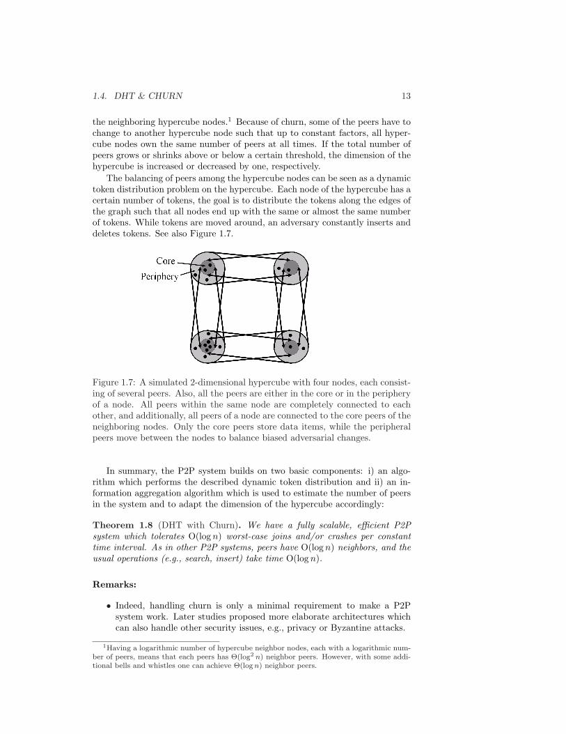
The balancing of peers among the hypercube nodes can be seen as a dynamictoken distribution problem on the hypercube. Each node of the hypercube has acertain number of tokens, the goal is to distribute the tokens along the edges ofthe graph such that all nodes end up with the same or almost the same numberof tokens. While tokens are moved around, an adversary constantly inserts anddeletes tokens. See also Figure 1.7.
Figure 1.7: A simulated 2-dimensional hypercube with four nodes, each consist-ing of several peers. Also, all the peers are either in the core or in the peripheryof a node. All peers within the same node are completely connected to eachother, and additionally, all peers of a node are connected to the core peers of theneighboring nodes. Only the core peers store data items, while the peripheralpeers move between the nodes to balance biased adversarial changes.
In summary, the P2P system builds on two basic components: i) an algo-rithm which performs the described dynamic token distribution and ii) an in-formation aggregation algorithm which is used to estimate the number of peersin the system and to adapt the dimension of the hypercube accordingly:
Theorem 1.8 (DHT with Churn). We have a fully scalable, efficient P2Psystem which tolerates O(log n) worst-case joins and/or crashes per constanttime interval. As in other P2P systems, peers have O(log n) neighbors, and theusual operations (e.g., search, insert) take time O(log n).
Remarks:
• Indeed, handling churn is only a minimal requirement to make a P2Psystem work. Later studies proposed more elaborate architectures whichcan also handle other security issues, e.g., privacy or Byzantine attacks.
1Having a logarithmic number of hypercube neighbor nodes, each with a logarithmic num-ber of peers, means that each peers has Θ(log2 n) neighbor peers. However, with some addi-tional bells and whistles one can achieve Θ(log n) neighbor peers.
14 CHAPTER 1. COMMUNICATION NETWORKS
• It is surprising that unstructured (in fact, hybrid) P2P systems dominatestructured P2P systems in the real world. One would think that structuredP2P systems have advantages, in particular their efficient logarithmic datalookup. On the other hand, unstructured P2P networks are simpler, inparticular in light of non-exact queries.

Chapter 2
Leader Election
2.1 Distributed Algorithms and Complexity
In the second part of this course we will often model the distributed system as anetwork or graph, and study protocols in which nodes (i.e., the processors) canonly communicate with their neighbors to perform certain tasks. We are ofteninterested in the following synchronous model or algorithm.
Definition 2.1 (Synchronous Distributed Algorithm). In a synchronous al-gorithm, nodes operate in synchronous rounds. In each round, each processorexecutes the following steps:
1. Do some local computation (of reasonable “local complexity”).
2. Send messages to neighbors in graph (of reasonable size).
3. Receive messages (that were sent by neighbors in step 2 of the same round).
Remarks:
• Any other step ordering is fine.
The other cornerstone model is the asynchronous algorithm.
Definition 2.2 (Asynchronous Distributed Algorithm). In the asynchronousmodel, algorithms are event driven (“upon receiving message . . . , do . . . ”).Processors cannot access a global clock. A message sent from one processorto another will arrive in finite but unbounded time.
Remarks:
• The asynchronous model and the synchronous model (Definition 2.1) arethe cornerstone models in distributed computing. As they do not neces-sarily reflect reality there are several models in between synchronous andasynchronous. However, from a theoretical point of view the synchronousand the asynchronous model are the most interesting ones (because everyother model is in between these extremes).
• Note that in the asynchronous model, messages that take a longer pathmay arrive earlier.
15

16 CHAPTER 2. LEADER ELECTION
In order to evaluate an algorithm, apart from the local complexity mentionedabove, we consider the following metrics.
Definition 2.3 (Time Complexity). For synchronous algorithms (as defined in2.1) the time complexity is the number of rounds until the algorithm terminates.
Definition 2.4 (Time Complexity). For asynchronous algorithms (as definedin 2.1) the time complexity is the number of time units from the start of theexecution to its completion in the worst case (every legal input, every executionscenario), assuming that each message has a delay of at most one time unit.
Remarks:
• You cannot use the maximum delay in the algorithm design. In otherwords, the algorithm has to be correct even if there is no such delay upperbound.
Definition 2.5 (Message Complexity). The message complexity of a syn-chronous and asynchronous algorithm is determined by the number of messagesexchanged (again every legal input, every execution scenario).
2.2 Anonymous Leader Election
Some algorithms (e.g., for medium access) ask for a special node, a so-called“leader”. Computing a leader is a most simple form of symmetry breaking. Al-gorithms based on leaders do generally not exhibit a high degree of parallelism,and therefore often suffer from poor (parallel) time complexity. However, some-times it is still useful to have a leader to make critical decisions in an easy(though non-distributed!) way.
The process of choosing a leader is known as leader election. Although leaderelection is a simple form of symmetry breaking, there are some remarkable issuesthat allow us to introduce notable computational models.
In this chapter we concentrate on the ring topology. The ring is the “dro-sophila” of distributed computing as many interesting challenges already revealthe root of the problem in the special case of the ring. Paying special attentionto the ring also makes sense from a practical point of view as some real worldsystems are based on a ring topology, e.g., the token ring standard for local areanetworks.
Problem 2.6 (Leader Election). Each node eventually decides whether it is aleader or not, subject to the constraint that there is exactly one leader.
Remarks:
• More formally, nodes are in one of three states: undecided, leader, notleader. Initially every node is in the undecided state. When leaving theundecided state, a node goes into a final state (leader or not leader).
Definition 2.7 (Anonymous). A system is anonymous if nodes do not haveunique identifiers.
2.3. ASYNCHRONOUS RING 17
Definition 2.8 (Uniform). An algorithm is called uniform if the number ofnodes n is not known to the algorithm (to the nodes, if you wish). If n isknown, the algorithm is called non-uniform.
Whether a leader can be elected in an anonymous system depends on whetherthe network is symmetric (ring, complete graph, complete bipartite graph, etc.)or asymmetric (star, single node with highest degree, etc.). Simplifying slightly,in this context a symmetric graph is a graph in which the extended neighborhoodof each node has the same structure. We will now show that non-uniformanonymous leader election for synchronous rings is impossible. The idea is thatin a ring, symmetry can always be maintained.
Lemma 2.9. After round k of any deterministic algorithm on an anonymousring, each node is in the same state sk.
Proof by induction: All nodes start in the same state. A round in a synchronousalgorithm consists of the three steps sending, receiving, local computation (seeDefinition 2.1). All nodes send the same message(s), receive the same mes-sage(s), do the same local computation, and therefore end up in the same state.
Theorem 2.10 (Anonymous Leader Election). Deterministic leader election inan anonymous ring is impossible.
Proof (with Lemma 2.9): If one node ever decides to become a leader (or anon-leader), then every other node does so as well, contradicting the problemspecification 2.6 for n > 1. This holds for non-uniform algorithms, and thereforealso for uniform algorithms. Furthermore, it holds for synchronous algorithms,and therefore also for asynchronous algorithms.
Remarks:
• Sense of direction is the ability of nodes to distinguish neighbor nodes inan anonymous setting. In a ring, for example, a node can distinguish theclockwise and the counterclockwise neighbor. Sense of direction does nothelp in anonymous leader election.
• Theorem 2.10 also holds for other symmetric network topologies (e.g.,complete graphs, complete bipartite graphs, . . . ).
• Note that Theorem 2.10 does not hold for randomized algorithms; if nodesare allowed to toss a coin, symmetries can be broken.
2.3 Asynchronous Ring
We first concentrate on the asynchronous model from Definition 2.2. Through-out this section we assume non-anonymity; each node has a unique identifier asproposed in Assumption 4.2:
Assumption 2.11 (Node Identifiers). Each node has a unique identifier, e.g.,its IP address. We usually assume that each identifier consists of only log n bitsif the system has n nodes.
Having ID’s seems to lead to a trivial leader election algorithm, as we cansimply elect the node with, e.g., the highest ID.
18 CHAPTER 2. LEADER ELECTION
Algorithm 1 Clockwise1: Each node v executes the following code:2: v sends a message with its identifier (for simplicity also v) to its clockwise
neighbor. If node v already received a message w with w > v, then nodev can skip this step; if node v receives its first message w with w < v, thennode v will immediately send v.
3: if v receives a message w with w > v then4: v forwards w to its clockwise neighbor5: v decides not to be the leader, if it has not done so already.6: else if v receives its own identifier v then7: v decides to be the leader8: end if
Theorem 2.12 (Analysis of Algorithm 1). Algorithm 1 is correct. The timecomplexity is O(n). The message complexity is O(n2).
Proof: Let node z be the node with the maximum identifier. Node z sendsits identifier in clockwise direction, and since no other node can swallow it,eventually a message will arrive at z containing it. Then z declares itself tobe the leader. Every other node will declare non-leader at the latest whenforwarding message z. Since there are n identifiers in the system, each nodewill at most forward n messages, giving a message complexity of at most n2.We start measuring the time when the first node that “wakes up” sends itsidentifier. For asynchronous time complexity (Definition 2.4) we assume thateach message takes at most one time unit to arrive at its destination. After atmost n − 1 time units the message therefore arrives at node z, waking z up.Routing the message z around the ring takes at most n time units. Thereforenode z decides no later than at time 2n − 1. Every other node decides beforenode z.
Remarks:
• Note that in Algorithm 1 nodes need to distinguish between clockwiseand counterclockwise neighbors. In fact they do not: It is okay to simplysend your own identifier to any neighbor, and forward a message m to theneighbor you did not receive the message m from. So nodes only need tobe able to distinguish their two neighbors.
• Can we improve this algorithm?
Theorem 2.13 (Analysis of Algorithm 2). Algorithm 2 is correct. The timecomplexity is O(n). The message complexity is O(n log n).
Proof: Correctness is as in Theorem 2.12. The time complexity is O(n) sincethe node with maximum identifier z sends messages with round-trip times2, 4, 8, 16, . . . , 2 · 2k with k ≤ log(n + 1). (Even if we include the additionalwake-up overhead, the time complexity stays linear.) Proving the message com-plexity is slightly harder: if a node v manages to survive round r, no other nodein distance 2r (or less) survives round r. That is, node v is the only node in its2r-neighborhood that remains active in round r + 1. Since this is the same forevery node, less than n/2r nodes are active in round r+1. Being active in round

2.4. LOWER BOUNDS 19
Algorithm 2 Radius Growth (For readability we provide pseudo-code only; fora formal version please consult [Attiya/Welch Alg. 3.1])1: Each node v does the following:2: Initially all nodes are active. all nodes may still become leaders3: Whenever a node v sees a message w with w > v, then v decides to not be
a leader and becomes passive.4: Active nodes search in an exponentially growing neighborhood (clockwise
and counterclockwise) for nodes with higher identifiers, by sending out probemessages. A probe message includes the ID of the original sender, a bitwhether the sender can still become a leader, and a time-to-live number(TTL). The first probe message sent by node v includes a TTL of 1.
5: Nodes (active or passive) receiving a probe message decrement the TTL andforward the message to the next neighbor; if their ID is larger than the onein the message, they set the leader bit to zero, as the probing node doesnot have the maximum ID. If the TTL is zero, probe messages are returnedto the sender using a reply message. The reply message contains the ID ofthe receiver (the original sender of the probe message) and the leader-bit.Reply messages are forwarded by all nodes until they reach the receiver.
6: Upon receiving the reply message: If there was no node with higher IDin the search area (indicated by the bit in the reply message), the TTL isdoubled and two new probe messages are sent (again to the two neighbors).If there was a better candidate in the search area, then the node becomespassive.
7: If a node v receives its own probe message (not a reply) v decides to be theleader.
r costs 2 · 2 · 2r messages. Therefore, round r costs at most 2 · 2 · 2r · n2r−1 = 8n
messages. Since there are only logarithmic many possible rounds, the messagecomplexity follows immediately.
Remarks:
• This algorithm is asynchronous and uniform as well.
• The question may arise whether one can design an algorithm with an evenlower message complexity. We answer this question in the next section.
2.4 Lower Bounds
Lower bounds in distributed computing are often easier than in the standardcentralized (random access machine, RAM) model because one can argue aboutmessages that need to be exchanged. In this section we present a first lowerbound. We show that Algorithm 2 is asymptotically optimal.
Definition 2.14 (Execution). An execution of a distributed algorithm is a listof events, sorted by time. An event is a record (time, node, type, message),where type is “send” or “receive”.

20 CHAPTER 2. LEADER ELECTION
Remarks:
• We assume throughout this course that no two events happen at exactlythe same time (or one can break ties arbitrarily).
• An execution of an asynchronous algorithm is generally not only deter-mined by the algorithm but also by a “god-like” scheduler. If more thanone message is in transit, the scheduler can choose which one arrives first.
• If two messages are transmitted over the same directed edge, then it issometimes required that the message first transmitted will also be receivedfirst (“FIFO”).
For our lower bound, we assume the following model:
• We are given an asynchronous ring, where nodes may wake up at arbitrarytimes (but at the latest when receiving the first message).
• We only accept uniform algorithms where the node with the maximumidentifier can be the leader. Additionally, every node that is not theleader must know the identity of the leader. These two requirements canbe dropped when using a more complicated proof; however, this is beyondthe scope of this course.
• During the proof we will “play god” and specify which message in trans-mission arrives next in the execution. We respect the FIFO conditions forlinks.
Definition 2.15 (Open Schedule). A schedule is an execution chosen by thescheduler. A schedule for a ring is open if there is an open edge in the ring.An open (undirected) edge is an edge where no message traversing the edge hasbeen received so far.
The proof of the lower bound is by induction. First we show the base case:
Lemma 2.16. Given a ring R with two nodes, we can construct an open sched-ule in which at least one message is received. The nodes cannot distinguish thisschedule from one on a larger ring with all other nodes being where the openedge is.
Proof: Let the two nodes be u and v with u < v. Node u must learn theidentity of node v, thus receive at least one message. We stop the execution ofthe algorithm as soon as the first message is received. (If the first message isreceived by v, bad luck for the algorithm!) Then the other edge in the ring (onwhich the received message was not transmitted) is open. Since the algorithmneeds to be uniform, maybe the open edge is not really an edge at all, nobodycan tell. We could use this to glue two rings together, by breaking up thisimaginary open edge and connect two rings by two edges.
Lemma 2.17. By gluing together two rings of size n/2 for which we have openschedules, we can construct an open schedule on a ring of size n. If M(n/2)denotes the number of messages already received in each of these schedules, atleast 2M(n/2) + n/4 messages have to be exchanged in order to solve leaderelection.

2.5. SYNCHRONOUS RING 21
Proof by induction: We divide the ring into two sub-rings R1 and R2 of sizen/2. These subrings cannot be distinguished from rings with n/2 nodes if nomessages are received from “outsiders”. We can ensure this by not schedulingsuch messages until we want to. Note that executing both given open scheduleson R1 and R2 “in parallel” is possible because we control not only the schedulingof the messages, but also when nodes wake up. By doing so, we make sure that2M(n/2) messages are sent before the nodes in R1 and R2 learn anything ofeach other!
Without loss of generality, R1 contains the maximum identifier. Hence, eachnode in R2 must learn the identity of the maximum identifier, thus at leastn/2 additional messages must be received. The only problem is that we cannotconnect the two sub-rings with both edges since the new ring needs to remainopen. Thus, only messages over one of the edges can be received. We “playgod” and look into the future: we check what happens when we close only oneof these connecting edges. With the argument that n/2 new messages must bereceived, we know that there is at least one edge that will produce at least n/4additional messages when being scheduled. (These messages may not be sentover the closed link, but they are caused by a message over this link. Theycannot involve any message along the other (open) edge at distance n/2.) Weschedule this edge and the resulting n/4 messages, and leave the other open.
Lemma 2.18. Any uniform leader election algorithm for asynchronous ringshas at least message complexity M(n) ≥ n
4 (log n + 1).
Proof by induction: For simplicity we assume n being a power of 2. The basecase n = 2 works because of Lemma 2.16 which implies that M(2) ≥ 1 =24 (log 2 + 1). For the induction step, using Lemma 2.17 and the inductionhypothesis we have
M(n) = 2 ·M(n
2
)+
n
4
≥ 2 ·(n
8
(log
n
2+ 1
))+
n
4=
n
4log n +
n
4=
n
4(log n + 1) .
2
Remarks:
• To hide the ugly constants we use the “big Omega” notation, the lowerbound equivalent of O(). A function f is in Ω(g) if there are constantsx0 and c > 0 such that |f(x)| ≥ c|g(x)| for all x ≥ x0. Again we referto standard text books for a formal definition. Rewriting Lemma 2.18 weget:
Theorem 2.19 (Asynchronous Leader Election Lower Bound). Any uniformleader election algorithm for asynchronous rings has Ω(n log n) message com-plexity.
2.5 Synchronous Ring
The lower bound relied on delaying messages for a very long time. Since this isimpossible in the synchronous model, we might get a better message complexity

22 CHAPTER 2. LEADER ELECTION
in this case. The basic idea is very simple: In the synchronous model, notreceiving a message is information as well! First we make some additionalassumptions:
• We assume that the algorithm is non-uniform (i.e., the ring size n isknown).
• We assume that every node starts at the same time.
• The node with the minimum identifier becomes the leader; identifiers areintegers.
Algorithm 3 Synchronous Leader Election1: Each node v concurrently executes the following code:2: The algorithm operates in synchronous phases. Each phase consists of n
time steps. Node v counts phases, starting with 0.3: if phase = v and v did not yet receive a message then4: v decides to be the leader5: v sends the message “v is leader” around the ring6: end if
Remarks:
• Message complexity is indeed n.
• But the time complexity is huge! If m is the minimum identifier it is m ·n.
• The synchronous start and the non-uniformity assumptions can be drop-ped by using a wake-up technique (upon receiving a wake-up message,wake up your clockwise neighbors) and by letting messages travel slowly.
• There are several lower bounds for the synchronous model: comparison-based algorithms or algorithms where the time complexity cannot be afunction of the identifiers have message complexity Ω(n log n) as well.
• In general graphs efficient leader election may be tricky. While time-optimal leader election can be done by parallel flooding-echo (see nextchapter), bounding the message complexity is generally more difficult.

Chapter 3
Tree Algorithms
In this chapter we learn a few basic algorithms on trees, and how to constructtrees in the first place so that we can run these (and other) algorithms. Thegood news is that these algorithms have many applications, the bad news isthat this chapter is a bit on the simple side. But maybe that’s not really badnews?!
3.1 Broadcast
Definition 3.1 (Broadcast). A broadcast operation is initiated by a single pro-cessor, the source. The source wants to send a message to all other nodes inthe system.
Definition 3.2 (Distance, Radius, Diameter). The distance between two nodesu and v in an undirected graph G is the number of hops of a minimum pathbetween u and v. The radius of a node u is the maximum distance between uand any other node in the graph. The radius of a graph is the minimum radiusof any node in the graph. The diameter of a graph is the maximum distancebetween two arbitrary nodes.
Remarks:
• Clearly there is a close relation between the radius R and the diameter Dof a graph, such as R ≤ D ≤ 2R.
• The world is often fascinated by graphs with a small radius. For example,movie fanatics study the who-acted-with-whom-in-the-same-movie graph.For this graph it has long been believed that the actor Kevin Bacon hasa particularly small radius. The number of hops from Bacon even got aname, the Bacon Number. In the meantime, however, it has been shownthat there are “better” centers in the Hollywood universe, such as SeanConnery, Christopher Lee, Rod Steiger, Gene Hackman, or Michael Caine.The center of other social networks has also been explored, Paul Erdos forinstance is well known in the math community.
Theorem 3.3 (Broadcast Lower Bound). The message complexity of broadcastis at least n− 1. The source’s radius is a lower bound for the time complexity.
23

24 CHAPTER 3. TREE ALGORITHMS
Proof: Every node must receive the message.
Remarks:
• You can use a pre-computed spanning tree to do broadcast with tightmessage complexity. If the spanning tree is a breadth-first search spanningtree (for a given source), then the time complexity is tight as well.
Definition 3.4 (Clean). A graph (network) is clean if the nodes do not knowthe topology of the graph.
Theorem 3.5 (Clean Broadcast Lower Bound). For a clean network, the num-ber of edges is a lower bound for the broadcast message complexity.
Proof: If you do not try every edge, you might miss a whole part of the graphbehind it.
Remarks:
• This lower bound proof directly brings us to the well known flooding al-gorithm.
Algorithm 4 Flooding1: The source (root) sends the message to all neighbors.2: Each other node v upon receiving the message the first time forwards the
message to all (other) neighbors.3: Upon later receiving the message again (over other edges), a node can dis-
card the message.
Remarks:
• If node v receives the message first from node u, then node v calls nodeu parent. This parent relation defines a spanning tree T . If the floodingalgorithm is executed in a synchronous system, then T is a breadth-firstsearch spanning tree (with respect to the root).
• More interestingly, also in asynchronous systems the flooding algorithmterminates after R time units, R being the radius of the source. However,the constructed spanning tree may not be a breadth-first search spanningtree.
3.2 Convergecast
Convergecast is the same as broadcast, just reversed: Instead of a root sendinga message to all other nodes, all other nodes send information to a root. Thesimplest convergecast algorithm is the echo algorithm:

3.3. BFS TREE CONSTRUCTION 25
Algorithm 5 EchoRequire: This algorithm is initiated at the leaves.1: A leave sends a message to its parent.2: If an inner node has received a message from each child, it sends a message
to the parent.
Remarks:
• Usually the echo algorithm is paired with the flooding algorithm, which isused to let the leaves know that they should start the echo process; thisis known as flooding/echo.
• One can use convergecast for termination detection, for example. If a rootwants to know whether all nodes in the system have finished some task, itinitiates a flooding/echo; the message in the echo algorithm then means“This subtree has finished the task.”
• Message complexity of the echo algorithm is n − 1, but together withflooding it is O(m), where m = |E| is the number of edges in the graph.
• The time complexity of the echo algorithm is determined by the depth ofthe spanning tree (i.e., the radius of the root within the tree) generatedby the flooding algorithm.
• The flooding/echo algorithm can do much more than collecting acknowl-edgements from subtrees. One can for instance use it to compute thenumber of nodes in the system, or the maximum ID (for leader election),or the sum of all values stored in the system, or a route-disjoint matching.
• Moreover, by combining results one can compute even fancier aggrega-tions, e.g., with the number of nodes and the sum one can compute theaverage. With the average one can compute the standard deviation. Andso on . . .
3.3 BFS Tree Construction
In synchronous systems the flooding algorithm is a simple yet efficient method toconstruct a breadth-first search (BFS) spanning tree. However, in asynchronoussystems the spanning tree constructed by the flooding algorithm may be far fromBFS. In this section, we implement two classic BFS constructions—Dijkstra andBellman-Ford—as asynchronous algorithms.
We start with the Dijkstra algorithm. The basic idea is to always add the“closest” node to the existing part of the BFS tree. We need to parallelize thisidea by developing the BFS tree layer by layer:
Theorem 3.6 (Analysis of Algorithm 6). The time complexity of Algorithm 6is O(D2), the message complexity is O(m + nD), where D is the diameter ofthe graph, n the number of nodes, and m the number of edges.
Proof: A broadcast/echo algorithm in Tp needs at most time 2D. Finding newneighbors at the leaves costs 2 time units. Since the BFS tree height is bounded

26 CHAPTER 3. TREE ALGORITHMS
Algorithm 6 Dijkstra BFS1: The algorithm proceeds in phases. In phase p the nodes with distance p to
the root are detected. Let Tp be the tree in phase p. We start with T1 whichis the root plus all direct neighbors of the root. We start with phase p = 1:
2: repeat3: The root starts phase p by broadcasting “start p” within Tp.4: When receiving “start p” a leaf node u of Tp (that is, a node that was
newly discovered in the last phase) sends a “join p + 1” message to allquiet neighbors. (A neighbor v is quiet if u has not yet “talked” to v.)
5: A node v receiving the first “join p+1” message replies with “ACK” andbecomes a leaf of the tree Tp+1.
6: A node v receiving any further “join” message replies with “NACK”.7: The leaves of Tp collect all the answers of their neighbors; then the leaves
start an echo algorithm back to the root.8: When the echo process terminates at the root, the root increments the
phase9: until there was no new node detected
by the diameter, we have D phases, giving a total time complexity of O(D2).Each node participating in broadcast/echo only receives (broadcasts) at most 1message and sends (echoes) at most once. Since there are D phases, the cost isbounded by O(nD). On each edge there are at most 2 “join” messages. Repliesto a “join” request are answered by 1 “ACK” or “NACK” , which means that wehave at most 4 additional messages per edge. Therefore the message complexityis O(m + nD).
Remarks:
• The time complexity is not very exciting, so let’s try Bellman-Ford!
The basic idea of Bellman-Ford is even simpler, and heavily used in theInternet, as it is a basic version of the omnipresent border gateway protocol(BGP). The idea is to simply keep the distance to the root accurate. If aneighbor has found a better route to the root, a node might also need to updateits distance.
Algorithm 7 Bellman-Ford BFS1: Each node u stores an integer du which corresponds to the distance from u
to the root. Initially droot = 0, and du = ∞ for every other node u.2: The root starts the algorithm by sending “1” to all neighbors.3: if a node u receives a message “y” with y < du from a neighbor v then4: node u sets du := y5: node u sends “y + 1” to all neighbors (except v)6: end if
Theorem 3.7 (Analysis of Algorithm 7). The time complexity of Algorithm7 is O(D), the message complexity is O(nm), where D, n,m are defined as inTheorem 3.6.
Proof: We can prove the time complexity by induction. We claim that a nodeat distance d from the root has received a message “d” by time d. The root

3.4. MST CONSTRUCTION 27
knows by time 0 that it is the root. A node v at distance d has a neighbor uat distance d− 1. Node u by induction sends a message “d” to v at time d− 1or before, which is then received by v at time d or before. Message complexityis easier: A node can reduce its distance at most n − 1 times; each of thesetimes it sends a message to all its neighbors. If all nodes do this we have O(nm)messages.
Remarks:
• Algorithm 6 has the better message complexity and Algorithm 7 has thebetter time complexity. The currently best algorithm (optimizing both)needs O(m + n log3 n) messages and O(D log3 n) time. This “trade-off”algorithm is beyond the scope of this course.
3.4 MST Construction
There are several types of spanning trees, each serving a different purpose. Aparticularly interesting spanning tree is the minimum spanning tree (MST). TheMST only makes sense on weighted graphs, hence in this section we assume thateach edge e is assigned a weight ωe.
Definition 3.8 (MST). Given a weighted graph G = (V, E, ω), the MST of G isa spanning tree T minimizing ω(T ), where ω(G′) =
∑e∈G′ ωe for any subgraph
G′ ⊆ G.
Remarks:
• In the following we assume that no two edges of the graph have the sameweight. This simplifies the problem as it makes the MST unique; however,this simplification is not essential as one can always break ties by addingthe IDs of adjacent vertices to the weight.
• Obviously we are interested in computing the MST in a distributed way.For this we use a well-known lemma:
Definition 3.9 (Blue Edges). Let T be a spanning tree of the weighted graphG and T ′ ⊆ T a subgraph of T (also called a fragment). Edge e = (u, v) is anoutgoing edge of T ′ if u ∈ T ′ and v /∈ T ′ (or vice versa). The minimum weightoutgoing edge b(T ′) is the so-called blue edge of T ′.
Lemma 3.10. For a given weighted graph G (such that no two weights are thesame), let T denote the MST, and T ′ be a fragment of T . Then the blue edgeof T ′ is also part of T , i.e., T ′ ∪ b(T ′) ⊆ T .
Proof: For the sake of contradiction, suppose that in the MST T there is edgee 6= b(T ′) connecting T ′ with the remainder of T . Adding the blue edge b(T ′) tothe MST T we get a cycle including both e and b(T ′). If we remove e from thiscycle we still have a spanning tree, and since by the definition of the blue edgeωe > ωb(T ′), the weight of that new spanning tree is less than than the weightof T . We have a contradiction.

28 CHAPTER 3. TREE ALGORITHMS
Remarks:
• In other words, the blue edges seem to be the key to a distributed al-gorithm for the MST problem. Since every node itself is a fragment ofthe MST, every node directly has a blue edge! All we need to do is togrow these fragments! Essentially this is a distributed version of Kruskal’ssequential algorithm.
• At any given time the nodes of the graph are partitioned into fragments(rooted subtrees of the MST). Each fragment has a root, the ID of thefragment is the ID of its root. Each node knows its parent and its childrenin the fragment. The algorithm operates in phases. At the beginning of aphase, nodes know the IDs of the fragments of their neighbor nodes.
Algorithm 8 GHS (Gallager–Humblet–Spira)1: Initially each node is the root of its own fragment. We proceed in phases:2: repeat3: All nodes learn the fragment IDs of their neighbors.4: The root of each fragment uses flooding/echo in its fragment to determine
the blue edge b = (u, v) of the fragment.5: The root sends a message to node u; while forwarding the message on the
path from the root to node u all parent-child relations are inverted suchthat u is the new temporary root of the fragment
6: node u sends a merge request over the blue edge b = (u, v).7: if node v also sent a merge request over the same blue edge b = (v, u)
then8: either u or v (whichever has the smaller ID) is the new fragment root9: the blue edge b is directed accordingly
10: else11: node v is the new parent of node u12: end if13: the newly elected root node informs all nodes in its fragment (again using
flooding/echo) about its identity14: until all nodes are in the same fragment (i.e., there is no outgoing edge)
Remarks:
• Algorithm 8 was stated in pseudo-code, with a few details not really ex-plained. For instance, it may be that some fragments are much largerthan others, and because of that some nodes may need to wait for others,e.g., if node u needs to find out whether neighbor v also wants to mergeover the blue edge b = (u, v). The good news is that all these details canbe solved. We can for instance bound the asynchronicity by guaranteeingthat nodes only start the new phase after the last phase is done, similarlyto the phase-technique of Algorithm 6.
Theorem 3.11 (Analysis of Algorithm 8). The time complexity of Algorithm8 is O(n log n), the message complexity is O(m log n).
Proof: Each phase mainly consists of two flooding/echo processes. In general,the cost of flooding/echo on a tree is O(D) time and O(n) messages. However,

3.4. MST CONSTRUCTION 29
the diameter D of the fragments may turn out to be not related to the diameterof the graph because the MST may meander, hence it really is O(n) time. Inaddition, in the first step of each phase, nodes need to learn the fragment ID oftheir neighbors; this can be done in 2 steps but costs O(m) messages. There area few more steps, but they are cheap. Altogether a phase costs O(n) time andO(m) messages. So we only have to figure out the number of phases: Initially allfragments are single nodes and hence have size 1. In a later phase, each fragmentmerges with at least one other fragment, that is, the size of the smallest fragmentat least doubles. In other words, we have at most log n phases. The theoremfollows directly.
Remarks:
• Algorithm 8 is called “GHS” after Gallager, Humblet, and Spira, three pi-oneers in distributed computing. Despite being quite simple the algorithmwon the prestigious Edsger W. Dijkstra Prize in Distributed Computingin 2004, among other reasons because it was one of the first (1983) non-trivial asynchronous distributed algorithms. As such it can be seen as oneof the seeds of this research area.
• We presented a simplified version of GHS. The original paper by Gallageret al. featured an improved message complexity of O(m + n log n).
• In 1987, Awerbuch managed to further improve the GHS algorithm to getO(n) time and O(m + n log n) message complexity, both asymptoticallyoptimal.
• The GHS algorithm can be applied in different ways. GHS for instancedirectly solves leader election in general graphs: The leader is simply thelast surviving root!

30 CHAPTER 3. TREE ALGORITHMS

Chapter 4
Vertex Coloring
4.1 Introduction
Vertex coloring is an infamous graph theory problem. Vertex coloring does havequite a few practical applications, for example in the area of wireless networkswhere coloring is the foundation of so-called TDMA MAC protocols. Generallyspeaking, vertex coloring is used as a means to break symmetries, one of themain themes in distributed computing. In this chapter we will not really talkabout vertex coloring applications but treat the problem abstractly. At the endof the class you probably learned the fastest (but not constant!) algorithm ever!Let us start with some simple definitions and observations.
Problem 4.1 (Vertex Coloring). Given an undirected graph G = (V,E), assigna color cu to each vertex u ∈ V such that the following holds: e = (v, w) ∈E ⇒ cv 6= cw.
Remarks:
• Throughout this course, we use the terms vertex and node interchangeably.
• The application often asks us to use few colors! In a TDMA MAC protocol,for example, less colors immediately imply higher throughput. However,in distributed computing we are often happy with a solution which is sub-optimal. There is a tradeoff between the optimality of a solution (efficacy),and the work/time needed to compute the solution (efficiency).
3
1 2
3
Figure 4.1: 3-colorable graph with a valid coloring.
31
32 CHAPTER 4. VERTEX COLORING
Assumption 4.2 (Node Identifiers). Each node has a unique identifier, e.g.,its IP address. We usually assume that each identifier consists of only log n bitsif the system has n nodes.
Remarks:
• Sometimes we might even assume that the nodes exactly have identifiers1, . . . , n.
• It is easy to see that node identifiers (as defined in Assumption 4.2) solvethe coloring problem 4.1, but not very well (essentially requiring n colors).How many colors are needed at least is a well-studied problem.
Definition 4.3 (Chromatic Number). Given an undirected Graph G = (V,E),the chromatic number χ(G) is the minimum number of colors to solve Problem4.1.
To get a better understanding of the vertex coloring problem, let us first lookat a simple non-distributed (“centralized”) vertex coloring algorithm:
Algorithm 9 Greedy Sequential1: while ∃ uncolored vertex v do2: color v with the minimal color (number) that does not conflict with the
already colored neighbors3: end while
Definition 4.4 (Degree). The number of neighbors of a vertex v, denoted byδ(v), is called the degree of v. The maximum degree vertex in a graph G definesthe graph degree ∆(G) = ∆.
Theorem 4.5 (Analysis of Algorithm 9). The algorithm is correct and termi-nates in n “steps”. The algorithm uses ∆ + 1 colors.
Proof: Correctness and termination are straightforward. Since each node has atmost ∆ neighbors, there is always at least one color free in the range 1, . . . , ∆+1.Remarks:
• For many graphs coloring can be done with much less than ∆ + 1 colors.
• This algorithm is not distributed at all; only one processor is active at atime. Still, maybe we can use the simple idea of Algorithm 9 to define adistributed coloring subroutine that may come in handy later.
Now we are ready to study distributed algorithms for this problem. The fol-lowing procedure can be executed by every vertex v in a distributed coloringalgorithm. The goal of this subroutine is to improve a given initial coloring.

4.2. COLORING TREES 33
Procedure 10 First FreeRequire: Node Coloring e.g., node IDs as defined in Assumption 4.2
Give v the smallest admissible color i.e., the smallest node color not used byany neighbor
Algorithm 11 Reduce1: Assume that initially all nodes have ID’s (Assumption 4.2)2: Each node v executes the following code3: node v sends its ID to all neighbors4: node v receives IDs of neighbors5: while node v has an uncolored neighbor with higher ID do6: node v sends “undecided” to all neighbors7: node v receives new decisions from neighbors8: end while9: node v chooses a free color using subroutine First Free (Procedure 10)
10: node v informs all its neighbors about its choice
Remarks:
• With this subroutine we have to make sure that two adjacent vertices arenot colored at the same time. Otherwise, the neighbors may at the sametime conclude that some small color c is still available in their neighbor-hood, and then at the same time decide to choose this color c.
Theorem 4.6 (Analysis of Algorithm 11). Algorithm 11 is correct and has timecomplexity n. The algorithm uses ∆ + 1 colors.
Remarks:
• Quite trivial, but also quite slow.
• However, it seems difficult to come up with a fast algorithm.
• Maybe it’s better to first study a simple special case, a tree, and then gofrom there.
4.2 Coloring Trees
Lemma 4.7. χ(Tree) ≤ 2
Constructive Proof: If the distance of a node to the root is odd (even), colorit 1 (0). An odd node has only even neighbors and vice versa. If we assumethat each node knows its parent (root has no parent) and children in a tree, thisconstructive proof gives a very simple algorithm:
Remarks:
• With the proof of Lemma 4.7, Algorithm 12 is correct.
• How can we determine a root in a tree if it is not already given? We willfigure that out later.

34 CHAPTER 4. VERTEX COLORING
31
100
5
31
2
5
Figure 4.2: Vertex 100 receives the lowest possible color.
Algorithm 12 Slow Tree Coloring1: Color the root 0, root sends 0 to its children2: Each node v concurrently executes the following code:3: if node v receives a message x (from parent) then4: node v chooses color cv = 1− x5: node v sends cv to its children (all neighbors except parent)6: end if
• The time complexity of the algorithm is the height of the tree.
• If the root was chosen unfortunately, and the tree has a degenerated topol-ogy, the time complexity may be up to n, the number of nodes.
• Also, this algorithm does not need to be synchronous . . . !
Theorem 4.8 (Analysis of Algorithm 12). Algorithm 12 is correct. If each nodeknows its parent and its children, the (asynchronous) time complexity is the treeheight which is bounded by the diameter of the tree; the message complexity isn− 1 in a tree with n nodes.
Remarks:
• In this case the asynchronous time complexity is the same as the syn-chronous time complexity.
• Nice trees, e.g. balanced binary trees, have logarithmic height, that is wehave a logarithmic time complexity.
• This algorithm is not very exciting. Can we do better than logarithmic?!?
The following algorithm terminates in log∗ n time. Log-Star?! That’s the num-ber of logarithms (to the base 2) you need to take to get down to at least 2,starting with n:
Definition 4.9 (Log-Star).∀x ≤ 2 : log∗ x := 1 ∀x > 2 : log∗ x := 1 + log∗(log x)

4.2. COLORING TREES 35
Remarks:
• Log-star is an amazingly slowly growing function. Log-star of all the atomsin the observable universe (estimated to be 1080) is 5! There are functionswhich grow even more slowly, such as the inverse Ackermann function,however, the inverse Ackermann function of all the atoms is 4. So log-starincreases indeed very slowly!
Here is the idea of the algorithm: We start with color labels that have log n bits.In each synchronous round we compute a new label with exponentially smallersize than the previous label, still guaranteeing to have a valid vertex coloring!But how are we going to do that?
Algorithm 13 “6-Color”1: Assume that initially the vertices are legally colored. Using Assumption 4.2
each label only has log n bits2: The root assigns itself the label 0.3: Each other node v executes the following code (synchronously in parallel)4: send cv to all children5: repeat6: receive cp from parent7: interpret cv and cp as little-endian bit-strings: c(k), . . . , c(1), c(0)8: let i be the smallest index where cv and cp differ9: the new label is i (as bitstring) followed by the bit cv(i) itself
10: send cv to all children11: until cw ∈ 0, . . . , 5 for all nodes w
Example:
Algorithm 13 executed on the following part of a tree:
Grand-parent 0010110000 → 10010 → . . .Parent 1010010000 → 01010 → 111Child 0110010000 → 10001 → 001
Theorem 4.10 (Analysis of Algorithm 13). Algorithm 13 terminates in log∗ ntime.
Proof: A detailed proof is, e.g., in [Peleg 7.3]. In class we do a sketch of theproof.
Remarks:
• Colors 11∗ (in binary notation, i.e., 6 or 7 in decimal notation) will not bechosen, because the node will then do another round. This gives a totalof 6 colors (i.e., colors 0,. . . , 5).
• Can one reduce the number of colors in only constant steps? Note thatalgorithm 11 does not work (since the degree of a node can be much higherthan 6)! For fewer colors we need to have siblings monochromatic!
• Before we explore this problem we should probably have a second look atthe end game of the algorithm, the UNTIL statement. Is this algorithmtruly local?! Let’s discuss!

36 CHAPTER 4. VERTEX COLORING
Algorithm 14 Shift Down1: Root chooses a new (different) color from 0, 1, 22: Each other node v concurrently executes the following code:3: Recolor v with the color of parent
Lemma 4.11 (Analysis of Algorithm 14). Algorithm 14 preserves coloring le-gality; also siblings are monochromatic.
Now Algorithm 11 (Reduce) can be used to reduce the number of used colorsfrom six to three.
Algorithm 15 Six-2-Three1: Each node v concurrently executes the following code:2: Run Algorithm 13 for log∗ n rounds.3: for x = 5, 4, 3 do4: Perform subroutine Shift down (Algorithm 14)5: if cv = x then6: choose new color cv ∈ 0, 1, 2 using subroutine First Free (Algorithm
10)7: end if8: end for
Theorem 4.12 (Analysis of Algorithm 15). Algorithm 15 colors a tree withthree colors in time O(log∗ n).
Remarks:
• The term O() used in Theorem 4.10 is called “big O” and is often usedin distributed computing. Roughly speaking, O(f) means “in the order off , ignoring constant factors and smaller additive terms.” More formally,for two functions f and g, it holds that f ∈ O(g) if there are constants x0
and c so that |f(x)| ≤ c|g(x)| for all x ≥ x0. For an elaborate discussionon the big O notation we refer to other introductory math or computerscience classes.
• As one can easily prove, a fast tree-coloring with only 2 colors is morethan exponentially more expensive than coloring with 3 colors. In a treedegenerated to a list, nodes far away need to figure out whether they arean even or odd number of hops away from each other in order to get a2-coloring. To do that one has to send a message to these nodes. Thiscosts time linear in the number of nodes.
• Also other lower bounds have been proved, e.g., any algorithm for 2-coloring the d-regular tree of radius r which runs in time at most 2r/3requires at least Ω(
√d) colors.
• The idea of this algorithm can be generalized, e.g., to a ring topology. Alsoa general graph with constant degree ∆ can be colored with ∆ + 1 colorsin O(log∗ n) time. The idea is as follows: In each step, a node comparesits label to each of its neighbors, constructing a logarithmic difference-tag

4.2. COLORING TREES 37
Figure 4.3: Possible execution of Algorithm 15.
as in 6-color (Algorithm 13). Then the new label is the concatenation ofall the difference-tags. For constant degree ∆, this gives a 3∆-label inO(log∗ n) steps. Algorithm 11 then reduces the number of colors to ∆+1in 23∆ (this is still a constant for constant ∆!) steps.
• Recently, researchers have proposed other methods to break down longID’s for log-star algorithms. With these new techniques, one is able tosolve other problems, e.g., a maximal independent set in bounded growthgraphs in O(log∗ n) time. These techniques go beyond the scope of thiscourse.
• Unfortunately, coloring a general graph is not yet possible with this tech-nique. We will see another technique for that in Chapter 5. With thistechnique it is possible to color a general graph with ∆ + 1 colors inO(log n) time.
• A lower bound by Linial shows that many of these log-star algorithms areasymptotically (up to constant factors) optimal. This lower bound uses aninteresting technique. However, because of the one-topic-per-class policywe cannot look at it today.

38 CHAPTER 4. VERTEX COLORING
Chapter 5
Maximal Independent Set
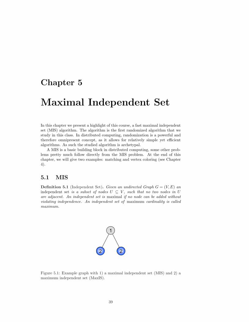
In this chapter we present a highlight of this course, a fast maximal independentset (MIS) algorithm. The algorithm is the first randomized algorithm that westudy in this class. In distributed computing, randomization is a powerful andtherefore omnipresent concept, as it allows for relatively simple yet efficientalgorithms. As such the studied algorithm is archetypal.
A MIS is a basic building block in distributed computing, some other prob-lems pretty much follow directly from the MIS problem. At the end of thischapter, we will give two examples: matching and vertex coloring (see Chapter4).
5.1 MIS
Definition 5.1 (Independent Set). Given an undirected Graph G = (V, E) anindependent set is a subset of nodes U ⊆ V , such that no two nodes in Uare adjacent. An independent set is maximal if no node can be added withoutviolating independence. An independent set of maximum cardinality is calledmaximum.
2
1
2
Figure 5.1: Example graph with 1) a maximal independent set (MIS) and 2) amaximum independent set (MaxIS).
39

40 CHAPTER 5. MAXIMAL INDEPENDENT SET
Remarks:
• Computing a maximum independent set (MaxIS) is a notoriously difficultproblem. It is equivalent to maximum clique on the complementary graph.Both problems are NP-hard, in fact not approximable within n
12−ε.
• In this course we concentrate on the maximal independent set (MIS) prob-lem. Please note that MIS and MaxIS can be quite different, indeed e.g.on a star graph the MIS is Θ(n) smaller than the MaxIS (cf. Figure 5.1).
• Computing a MIS sequentially is trivial: Scan the nodes in arbitrary order.If a node u does not violate independence, add u to the MIS. If u violatesindependence, discard u. So the only question is how to compute a MISin a distributed way.
Algorithm 16 Slow MISRequire: Node IDs
Every node v executes the following code:1: if all neighbors of v with larger identifiers have decided not to join the MIS
then2: v decides to join the MIS3: end if
Remarks:
• Not surprisingly the slow algorithm is not better than the sequential algo-rithm in the worst case, because there might be one single point of activityat any time. Formally:
Theorem 5.2 (Analysis of Algorithm 16). Algorithm 16 features a time com-plexity of O(n) and a message complexity of O(m).
Remarks:
• This is not very exciting.
• There is a relation between independent sets and node coloring (Chapter4), since each color class is an independent set, however, not necessarily aMIS. Still, starting with a coloring, one can easily derive a MIS algorithm:We first choose all nodes of the first color. Then, for each additional colorwe add “in parallel” (without conflict) as many nodes as possible. Thusthe following corollary holds:
Corollary 5.3. Given a coloring algorithm that needs C colors and runs intime T , we can construct a MIS in time C + T .
Remarks:
• Using Theorem 4.12 and Corollary 5.3 we get a distributed determinis-tic MIS algorithm for trees (and for bounded degree graphs) with timecomplexity O(log∗ n).
5.2. FAST MIS FROM 1986 41
• With a lower bound argument one can show that this deterministic MISalgorithm for rings is asymptotically optimal.
• There have been attempts to extend Algorithm 13 to more general graphs,however, so far without much success. Below we present a radically dif-ferent approach that uses randomization. Please note that the algorithmand the analysis below is not identical with the algorithm in Peleg’s book.
5.2 Fast MIS from 1986
Algorithm 17 Fast MISThe algorithm operates in synchronous rounds, grouped into phases.A single phase is as follows:1) Each node v marks itself with probability 1
2d(v) , where d(v) is the currentdegree of v.2) If no higher degree neighbor of v is also marked, node v joins the MIS. Ifa higher degree neighbor of v is marked, node v unmarks itself again. (If theneighbors have the same degree, ties are broken arbitrarily, e.g., by identifier).3) Delete all nodes that joined the MIS and their neighbors, as they cannotjoin the MIS anymore.
Remarks:
• Correctness in the sense that the algorithm produces an independent setis relatively simple: Steps 1 and 2 make sure that if a node v joins theMIS, then v’s neighbors do not join the MIS at the same time. Step 3makes sure that v’s neighbors will never join the MIS.
• Likewise the algorithm eventually produces a MIS, because the node withthe highest degree will mark itself at some point in Step 1.
• So the only remaining question is how fast the algorithm terminates. Tounderstand this, we need to dig a bit deeper.
Lemma 5.4 (Joining MIS). A node v joins the MIS in step 2 with probabilityp ≥ 1
4d(v) .
Proof: Let M be the set of marked nodes in step 1. Let H(v) be the set ofneighbors of v with higher degree, or same degree and higher identifier. Usingindependence of the random choices of v and nodes in H(v) in Step 1 we get
P [v /∈ MIS|v ∈ M ] = P [∃w ∈ H(v), w ∈ M |v ∈ M ]= P [∃w ∈ H(v), w ∈ M ]
≤∑
w∈H(v)
P [w ∈ M ] =∑
w∈H(v)
12d(w)
≤∑
w∈H(v)
12d(v)
≤ d(v)2d(v)
=12.
42 CHAPTER 5. MAXIMAL INDEPENDENT SET
Then
P [v ∈ MIS] = P [v ∈ MIS|v ∈ M ] · P [v ∈ M ] ≥ 12· 12d(v)
.
2
Lemma 5.5 (Good Nodes). A node v is called good if
∑
w∈N(v)
12d(w)
≥ 16.
Otherwise we call v a bad node. A good node will be removed in Step 3 withprobability p ≥ 1
36 .
Proof: Let node v be good. Intuitively, good nodes have lots of low-degreeneighbors, thus chances are high that one of them goes into the independentset, in which case v will be removed in step 3 of the algorithm.
If there is a neighbor w ∈ N(v) with degree at most 2 we are done: WithLemma 5.4 the probability that node w joins the MIS is at least 1
8 , and ourgood node will be removed in Step 3.
So all we need to worry about is that all neighbors have at least degree 3:
For any neighbor w of v we have 12d(w) ≤ 1
6 . Since∑
w∈N(v)
12d(w)
≥ 16
there is a
subset of neighbors S ⊆ N(v) such that16≤
∑
w∈S
12d(w)
≤ 13
We can now bound the probability that node v will be removed. Let thereforeR be the event of v being removed. Again, if a neighbor of v joins the MIS inStep 2, node v will be removed in Step 3. We have
P [R] ≥ P [∃u ∈ S, u ∈ MIS]
≥∑
u∈S
P [u ∈ MIS]−∑
u,w∈S;u 6=w
P [u ∈ MIS and w ∈ MIS] .
For the last inequality we used the inclusion-exclusion principle truncatedafter the second order terms. Let M again be the set of marked nodes afterStep 1. Using P [u ∈ M ] ≥ P [u ∈ MIS] we get
P [R] ≥∑
u∈S
P [u ∈ MIS]−∑
u,w∈S;u 6=w
P [u ∈ M and w ∈ M ]
≥∑
u∈S
P [u ∈ MIS]−∑
u∈S
∑
w∈S
P [u ∈ M ] · P [w ∈ M ]
≥∑
u∈S
14d(u)
−∑
u∈S
∑
w∈S
12d(u)
12d(w)
≥∑
u∈S
12d(u)
(12−
∑
w∈S
12d(w)
)≥ 1
6
(12− 1
3
)=
136
.
2

5.2. FAST MIS FROM 1986 43
Remarks:
• We would be almost finished if we could prove that many nodes are goodin each phase. Unfortunately this is not the case: In a star-graph, forinstance, only a single node is good! We need to find a work-around.
Lemma 5.6 (Good Edges). An edge e = (u, v) is called bad if both u and vare bad; else the edge is called good. The following holds: At any time at leasthalf of the edges are good.
Proof: For the proof we construct a directed auxiliary graph: Direct each edgetowards the higher degree node (if both nodes have the same degree direct ittowards the higher identifier). Now we need a little helper lemma before we cancontinue with the proof.
Lemma 5.7. A bad node has outdegree at least twice its indegree.
Proof: For the sake of contradiction, assume that a bad node v does not haveoutdegree at least twice its indegree. In other words, at least one third of theneighbor nodes (let’s call them S) have degree at most d(v). But then
∑
w∈N(v)
12d(w)
≥∑
w∈S
12d(w)
≥∑
w∈S
12d(v)
≥ d(v)3
12d(v)
=16
which means v is good, a contradiction. 2
Continuing the proof of Lemma 5.6: According to Lemma 5.7 the number ofedges directed into bad nodes is at most half the number of edges directed outof bad nodes. Thus, the number of edges directed into bad nodes is at mosthalf the number of edges. Thus, at least half of the edges are directed into goodnodes. Since these edges are not bad, they must be good.
Theorem 5.8 (Analysis of Algorithm 17). Algorithm 17 terminates in expectedtime O(log n).
Proof: With Lemma 5.5 a good node (and therefore a good edge!) will bedeleted with constant probability. Since at least half of the edges are good(Lemma 5.6) a constant fraction of edges will be deleted in each phase.
More formally: With Lemmas 5.5 and 5.6 we know that at least half of theedges will be removed with probability at least 1/36. Let R be the numberof edges to be removed. Using linearity of expectation we know that E [R] ≥m/72, m being the total number of edges at the start of a phase. Now letp := P [R ≤ E [R] /2]. Bounding the expectation yields
E [R] =∑
r
P [R = r] · r ≤ p · E [R] /2 + (1− p) ·m.
Solving for p we get
p ≤ m− E [R]m− E [R] /2
<m− E [R] /2
m≤ 1− 1/144.
In other words, with probability at least 1/144 at least m/144 edges are removedin a phase. After expected O(log m) phases all edges are deleted. Since m ≤ n2
and thus O(log m) = O(log n) the Theorem follows. 2

44 CHAPTER 5. MAXIMAL INDEPENDENT SET
Remarks:
• With a bit of more math one can even show that Algorithm 17 terminatesin time O(log n) “with high probability”.
• The presented algorithm is a simplified version of an algorithm by MichaelLuby, published 1986 in the SIAM Journal of Computing. Around thesame time there have been a number of other papers dealing with the sameor related problems, for instance by Alon, Babai, and Itai, or by Israeliand Itai. The analysis presented here takes elements of all these papers,and from other papers on distributed weighted matching. The analysis inthe book by David Peleg is different, and only achieves O(log2 n) time.
• Though not as incredibly fast as the log∗-coloring algorithm for trees, thisalgorithm is very general. It works on any graph, needs no identifiers, andcan easily be made asynchronous.
• Surprisingly, much later, there have been half a dozen more papers pub-lished, with much worse results!! In 2002, for instance, there was a paperwith linear running time, improving on a 1994 paper with cubic runningtime, restricted to trees!
• In 2009, Metivier, Robson, Saheb-Djahromi and Zemmari found a slightlydifferent (and simpler) way to compute a MIS in the same logarithmictime:
5.3 Fast MIS from 2009
Algorithm 18 Fast MIS 2The algorithm operates in synchronous rounds, grouped into phases.A single phase is as follows:1) Each node v chooses a random value r(v) ∈ [0, 1] and sends it to itsneighbors.2) If r(v) < r(w) for all neighbors w ∈ N(v), node v enters the MIS andinforms its neighbors.3) If v or a neighbor of v entered the MIS, v terminates (v and all edgesadjacent to v are removed from the graph), otherwise v enters the next phase.
Remarks:
• Correctness in the sense that the algorithm produces an independent setis simple: Steps 1 and 2 make sure that if a node v joins the MIS, thenv’s neighbors do not join the MIS at the same time. Step 3 makes surethat v’s neighbors will never join the MIS.
• Likewise the algorithm eventually produces a MIS, because the node withthe globally smallest value will always join the MIS, hence there is progress.
• So the only remaining question is how fast the algorithm terminates. Tounderstand this, we need to dig a bit deeper.

5.3. FAST MIS FROM 2009 45
• Our proof will rest on a simple, yet powerful observation about expectedvalues of random variables that may not be independent :
Theorem 5.9 (Linearity of Expectation). Let Xi, i = 1, . . . , k denote randomvariables, then
E
[∑
i
Xi
]=
∑
i
E [Xi] .
Proof. It is sufficient to prove E [X + Y ] = E [X]+E [Y ] for two random variablesX and Y , because then the statement follows by induction. Since
P [(X,Y ) = (x, y)] = P [X = x] · P [Y = y|X = x]= P [Y = y] · P [X = x|Y = y]
we get that
E [X + Y ] =∑
(X,Y )=(x,y)
P [(X, Y ) = (x, y)] · (x + y)
=∑
X=x
∑
Y =y
P [X = x] · P [Y = y|X = x] · x
+∑
Y =y
∑
X=x
P [Y = y] · P [X = x|Y = y] · y
=∑
X=x
P [X = x] · x +∑
Y =y
P [Y = y] · y
= E [X] + E [Y ] .
Remarks:
• How can we prove that the algorithm only needs O(log n) phases in expec-tation? It would be great if this algorithm managed to remove a constantfraction of nodes in each phase. Unfortunately, it does not.
• Instead we will prove that the number of edges decreases quickly. Again,it would be great if any single edge was removed with constant probabilityin Step 3. But again, unfortunately, this is not the case.
• Maybe we can argue about the expected number of edges to be removedin one single phase? Let’s see: A node v enters the MIS with probability1/(d(v) + 1), where d(v) is the degree of node v. By doing so, not onlyare v’s edges removed, but indeed all the edges of v’s neighbors as well –generally these are much more than d(v) edges. So there is hope, but weneed to be careful: If we do this the most naive way, we will count thesame edge many times.
• How can we fix this? The nice observation is that it is enough to countjust some of the removed edges. Given a new MIS node v and a neighborw ∈ N(v), we count the edges only if r(v) < r(x) for all x ∈ N(w). Thislooks promising. In a star graph, for instance, only the smallest randomvalue can be accounted for removing all the edges of the star.
46 CHAPTER 5. MAXIMAL INDEPENDENT SET
Lemma 5.10 (Edge Removal). In a single phase, we remove at least half ofthe edges in expectation.
Proof: To simplify the notation, at the start of our phase, the graph is simplyG = (V,E). Suppose that a node v joins the MIS in this phase, i.e., r(v) < r(w)for all neighbors w ∈ N(v). If in addition we have r(v) < r(x) for all neighborsx of a neighbor w of v, we call this event (v → w). The probability of event(v → w) is at least 1/(d(v) + d(w)), since d(v) + d(w) is the maximum numberof nodes adjacent to v or w (or both). As v joins the MIS, all edges (w, x) willbe removed; there are d(w) of these edges.
In order to count the removed edges, we need to weigh events properly.Whether we remove the edges adjacent to w because of event (v → w) is a
random variable X(v→w). If event (v → w) occurs, X(v→w) has the value d(w),if not it has the value 0. For each edge v, w we have two such variables, theevent X(v→w) and X(w→v). Due to Theorem 5.9, the expected value of the sumX of all these random variables is at least
E [X] =∑
v,w∈E
E[X(v→w)] + E[X(w→v)]
=∑
v,w∈E
P [Event (v → w)] · d(w) + P [Event (w → v)] · d(v)
≥∑
v,w∈E
d(w)d(v) + d(w)
+d(v)
d(w) + d(v)
=∑
v,w∈E
1 = |E|.
In other words, in expectation all edges are removed in a single phase?!?Probably not. This means that we still counted some edges more than once.Indeed, for an edge v, w ∈ E our random variable X includes the edge if theevent (u → v) happens, but X also includes the edge if the event (x → w)happens. So we may have counted the edge v, w twice. Fortunately however,not more than twice, because at most one event (· → v) and at most one event(· → w) can happen. If (u → v) happens, we know that r(u) < r(w) for allw ∈ N(v); hence another (u′ → v) cannot happen because r(u′) > r(u) ∈ N(v).Therefore the random variable X must be divided by 2. In other words, inexpectation at least half of the edges are removed.
Remarks:
• This enables us to follow a bound on the expected running time of Algo-rithm 18 quite easily.
Theorem 5.11 (Expected running time of Algorithm 18). Algorithm 18 ter-minates after at most 3 log4/3 m + 1 ∈ O(log n) phases in expectation.
Proof: The probability that in a single phase at least a quarter of all edgesare removed is at least 1/3. For the sake of contradiction, assume not. Thenwith probability less than 1/3 we may be lucky and many (potentially all) edgesare removed. With probability more than 2/3 less than 1/4 of the edges areremoved. Hence the expected fraction of removed edges is strictly less than1/3 · 1 + 2/3 · 1/4 = 1/2. This contradicts Lemma 5.10.

5.3. FAST MIS FROM 2009 47
Hence, at least every third phase is “good” and removes at least a quarterof the edges. To get rid of all but two edges we need log4/3 m good phases inexpectation. The last two edges will certainly be removed in the next phase.Hence a total of 3 log4/3 m + 1 phases are enough in expectation.
Remarks:
• Sometimes one expects a bit more of an algorithm: Not only should theexpected time to terminate be good, but the algorithm should alwaysterminate quickly. As this is impossible in randomized algorithms (afterall, the random choices may be “unlucky” all the time!), researchers oftensettle for a compromise, and just demand that the probability that thealgorithm does not terminate in the specified time can be made absurdlysmall. For our algorithm, this can be deduced from Lemma 5.10 andanother standard tool, namely Chernoff’s Bound.
Definition 5.12 (W.h.p.). We say that an algorithm terminates w.h.p. (withhigh probability) within O(t) time if it does so with probability at least 1− 1/nc
for any choice of c ≥ 1. Here c may affect the constants in the Big-O notationbecause it is considered a “tunable constant” and usually kept small.
Definition 5.13 (Chernoff’s Bound). Let X =∑k
i=1 Xi be the sum of k inde-pendent 0− 1 random variables. Then Chernoff’s bound states that w.h.p.
|X − E[X]| ∈ O(log n +
√E[X] log n
).
Corollary 5.14 (Running Time of Algorithm 18). Algorithm 18 terminatesw.h.p. in O(log n) time.
Proof: In Theorem 5.11 we used that independently of everything that happenedbefore, in each phase we have a constant probability p that a quarter of the edgesare removed. Call such a phase good. For some constants C1 and C2, let us checkafter C1 log n + C2 ∈ O(log n) phases, in how many phases at least a quarter ofthe edges have been removed. In expectation, these are at least p(C1 log n+C2)many. Now we look at the random variable X =
∑C1 log n+C2i=1 Xi, where the Xi
are independent 0− 1 variables being one with exactly probability p. Certainly,if X is at least x with some probability, then the probability that we havex good phases can only be larger (if no edges are left, certainly “all” of theremaining edges are removed). To X we can apply Chernoff’s bound. If C1
and C2 are chosen large enough, they will overcome the constants in the Big-Ofrom Chernoff’s bound, i.e., w.h.p. it holds that |X−E[X]| ≤ E[X]/2, implyingX ≥ E[X]/2. Choosing C1 large enough, we will have w.h.p. sufficiently manygood phases, i.e., the algorithm terminates w.h.p. in O(log n) phases.
Remarks:
• The algorithm can be improved a bit more even. Drawing random realnumbers in each phase for instance is not necessary. One can achievethe same by sending only a total of O(log n) random (and as many non-random) bits over each edge.
• One of the main open problems in distributed computing is whether onecan beat this logarithmic time, or at least achieve it with a deterministicalgorithm.

48 CHAPTER 5. MAXIMAL INDEPENDENT SET
• Let’s turn our attention to applications of MIS next.
5.4 Applications
Definition 5.15 (Matching). Given a graph G = (V,E) a matching is a subsetof edges M ⊆ E, such that no two edges in M are adjacent (i.e., where no nodeis adjacent to two edges in the matching). A matching is maximal if no edgecan be added without violating the above constraint. A matching of maximumcardinality is called maximum. A matching is called perfect if each node isadjacent to an edge in the matching.
Remarks:
• In contrast to MaxIS, a maximum matching can be found in polynomialtime (Blossom algorithm by Jack Edmonds), and is also easy to approxi-mate (in fact, already any maximal matching is a 2-approximation).
• An independent set algorithm is also a matching algorithm: Let G =(V,E) be the graph for which we want to construct the matching. Theauxiliary graph G′ is defined as follows: for every edge in G there is a nodein G′; two nodes in G′ are connected by an edge if their respective edgesin G are adjacent. A (maximal) independent set in G′ is a (maximal)matching in G, and vice versa. Using Algorithm 18 directly produces aO(log n) bound for maximal matching.
• More importantly, our MIS algorithm can also be used for vertex coloring(Problem 4.1):
Algorithm 19 General Graph Coloring1: Given a graph G = (V,E) we virtually build a graph G′ = (V ′, E′) as
follows:2: Every node v ∈ V clones itself d(v)+1 times (v0, . . . , vd(v) ∈ V ′), d(v) being
the degree of v in G.3: The edge set E′ of G′ is as follows:4: First all clones are in a clique: (vi, vj) ∈ E′, for all v ∈ V and all 0 ≤ i <
j ≤ d(v)5: Second all ith clones of neighbors in the original graph G are connected:
(ui, vi) ∈ E′, for all (u, v) ∈ E and all 0 ≤ i ≤ min(d(u), d(v)).6: Now we simply run (simulate) the fast MIS Algorithm 18 on G′.7: If node vi is in the MIS in G′, then node v gets color i.
Theorem 5.16 (Analysis of Algorithm 19). Algorithm 19 (∆ + 1)-colors anarbitrary graph in O(log n) time, with high probability, ∆ being the largest degreein the graph.
Proof: Thanks to the clique among the clones at most one clone is in the MIS.And because of the d(v)+1 clones of node v every node will get a free color! Therunning time remains logarithmic since G′ has O
(n2
)nodes and the exponent
becomes a constant factor when applying the logarithm.

5.4. APPLICATIONS 49
Remarks:
• This solves our open problem from Chapter 4.1!
• Together with Corollary 5.3 we get quite close ties between (∆+1)-coloringand the MIS problem.
• However, in general Algorithm 19 is not the best distributed algorithm forO(∆)-coloring. For fast distributed vertex coloring please check Kotha-palli, Onus, Scheideler, Schindelhauer, IPDPS 2006. This algorithm isbased on a O(log log n) time edge coloring algorithm by Grable and Pan-conesi, 1997.
• Computing a MIS also solves another graph problem on graphs of boundedindependence.
Definition 5.17 (Bounded Independence). G = (V, E) is of bounded indepen-dence, if each neighborhood contains at most a constant number of independent(i.e., mutually non-adjacent) nodes.
Definition 5.18 ((Minimum) Dominating Sets). A dominating set is a subsetof the nodes such that each node is in the set or adjacent to a node in the set.A minimum dominating set is a dominating set containing the least possiblenumber of nodes.
Remarks:
• In general, finding a dominating set less than factor log n larger than anminimum dominating set is NP-hard.
• Any MIS is a dominating set: if a node was not covered, it could join theindependent set.
• In general a MIS and a minimum dominating sets have not much in com-mon (think of a star). For graphs of bounded independence, this is differ-ent.
Corollary 5.19. On graphs of bounded independence, a constant-factor approx-imation to a minimum dominating set can be found in time O(log n) w.h.p.
Proof: Denote by M a minimum dominating set and by I a MIS. Since M is adominating set, each node from I is in M or adjacent to a node in M . Sincethe graph is of bounded independence, no node in M is adjacent to more thanconstantly many nodes from I. Thus, |I| ∈ O(|M |). Therefore, we can computea MIS with Algorithm 18 and output it as the dominating set, which takesO(log n) rounds w.h.p.

50 CHAPTER 5. MAXIMAL INDEPENDENT SET

Chapter 6
Locality Lower Bounds
In Chapter 4, we looked at distributed algorithms for coloring. In particular,we saw that rings and rooted trees can be colored with 3 colors in log∗ n+O(1)rounds. In this chapter, we will reconsider the distributed coloring problem. Wewill look at a classic lower bound by Nathan Linial that shows that the result ofChapter 4 is tight: Coloring rings (and rooted trees) indeed requires Ω(log∗ n)rounds. In particular, we will prove a lower bound for coloring in the followingsetting:
• We consider deterministic, synchronous algorithms.
• Message size and local computations are unbounded.
• We assume that the network is a directed ring with n nodes.
• Nodes have unique labels (identifiers) from 1 to n.
Remarks:
• A generalization of the lower bound to randomized algorithms is possible.Unfortunately, we will however not have time to discuss this.
• Except for restricting to deterministic algorithms, all the conditions abovemake a lower bound stronger. Any lower bound for synchronous algo-rithms certainly also holds for asynchronous ones. A lower bound that istrue if message size and local computations are not restricted is clearly alsovalid if we require a bound on the maximal message size or the amountof local computations. Similarly also assuming that the ring is directedand that node labels are from 1 to n (instead of choosing IDs from a moregeneral domain) strengthen the lower bound.
• Instead of directly proving that 3-coloring a ring needs Ω(log∗ n) rounds,we will prove a slightly more general statement. We will consider deter-ministic algorithms with time complexity r (for arbitrary r) and derive alower bound on the number of colors that are needed if we want to prop-erly color an n-node ring with an r-round algorithm. A 3-coloring lowerbound can then be derived by taking the smallest r for which an r-roundalgorithm needs 3 or fewer colors.
51

52 CHAPTER 6. LOCALITY LOWER BOUNDS
Algorithm 20 Synchronous Algorithm: Canonical Form1: In r rounds: send complete initial state to nodes at distance at most r2: // do all the communication first3: Compute output based on complete information about r-neighborhood4: // do all the computation in the end
6.1 Locality
Let us for a moment look at distributed algorithms more generally (i.e., notonly at coloring and not only at rings). Assume that initially, all nodes onlyknow their own label (identifier) and potentially some additional input. Asinformation needs at least r rounds to travel r hops, after r rounds, a node vcan only learn about other nodes at distance at most r. If message size and localcomputations are not restricted, it is in fact not hard to see, that in r rounds,a node v can exactly learn all the node labels and inputs up to distance r.As shown by the following lemma, this allows to transform every deterministicr-round synchronous algorithm into a simple canonical form.
Lemma 6.1. If message size and local computations are not bounded, everydeterministic, synchronous r-round algorithm can be transformed into an algo-rithm of the form given by Algorithm 20 (i.e., it is possible to first communicatefor r rounds and then do all the computations in the end).
Proof. Consider some r-round algorithm A. We want to show that A can bebrought to the canonical form given by Algorithm 20. First, we let the nodescommunicate for r rounds. Assume that in every round, every node sends itscomplete state to all of its neighbors (remember that there is no restriction onthe maximal message size). By induction, after r rounds, every node knows theinitial state of all other nodes at distance at most i. Hence, after r rounds, anode v has the combined initial knowledge of all the nodes in its r-neighborhood.We want to show that this suffices to locally (at node v) simulate enough ofAlgorithm A to compute all the messages that v receives in the r communicationrounds of a regular execution of Algorithm A.
Concretely, we prove the following statement by induction on i. For allnodes at distance at most r − i + 1 from v, node v can compute all messagesof the first i rounds of a regular execution of A. Note that this implies that vcan compute all the messages it receives from its neighbors during all r rounds.Because v knows the initial state of all nodes in the r-neighborhood, v canclearly compute all messages of the first round (i.e., the statement is true fori = 1). Let us now consider the induction step from i to i+1. By the inductionhypothesis, v can compute the messages of the first i rounds of all nodes inits (r − i + 1)-neighborhood. It can therefore compute all messages that arereceived by nodes in the (r − i)-neighborhood in the first i rounds. This is ofcourse exactly what is needed to compute the messages of round i + 1 of nodesin the (r − i)-neighborhood.

6.1. LOCALITY 53
Remarks:
• It is straightforward to generalize the canonical form to randomized algo-rithms: Every node first computes all the random bits it needs throughoutthe algorithm. The random bits are then part of the initial state of a node.
Definition 6.2 (r-hop view). We call the collection of the initial states of allnodes in the r-neighborhood of a node v, the r-hop view of v.
Remarks:
• Assume that initially, every node knows its degree, its label (identifier)and potentially some additional input. The r-hop view of a node v thenincludes the complete topology of the r-neighborhood (excluding edgesbetween nodes at distance r) and the labels and additional inputs of allnodes in the r-neighborhood.
Based on the definition of an r-hop view, we can state the following corollaryof Lemma 6.1.
Corollary 6.3. A deterministic r-round algorithm A is a function that mapsevery possible r-hop view to the set of possible outputs.
Proof. By Lemma 6.1, we know that we can transform Algorithm A to thecanonical form given by Algorithm 20. After r communication rounds, everynode v knows exactly its r-hop view. This information suffices to compute theoutput of node v.
Remarks:
• Note that the above corollary implies that two nodes with equal r-hopviews have to compute the same output in every r-round algorithm.
• For coloring algorithms, the only input of a node v is its label. The r-hopview of a node therefore is its labeled r-neighborhood.
• Since we only consider rings, r-hop neighborhoods are particularly simple.The labeled r-neighborhood of a node v (and hence its r-hop view) ina directed ring is simply a (2r + 1)-tuple (`−r, `−r+1, . . . , `0, . . . , `r) ofdistinct node labels where `0 is the label of v. Assume that for i > 0, `i
is the label of the ith clockwise neighbor of v and `−i is the label of theith counterclockwise neighbor of v. A deterministic coloring algorithm fordirected rings therefore is a function that maps (2r + 1)-tuples of nodelabels to colors.
• Consider two r-hop views Vr = (`−r, . . . , `r) and V ′r = (`′−r, . . . , `′r). If
`′i = `i+1 for −r ≤ i ≤ r − 1 and if `′r 6= `i for −r ≤ i ≤ r, the r-hop viewV ′r can be the r-hop view of a clockwise neighbor of a node with r-hop viewVr. Therefore, every algorithm A that computes a valid coloring needs toassign different colors to Vr and V ′r. Otherwise, there is a ring labeling forwhich A assigns the same color to two adjacent nodes.

54 CHAPTER 6. LOCALITY LOWER BOUNDS
6.2 The Neighborhood Graph
We will now make the above observations concerning colorings of rings a bitmore formal. Instead of thinking of an r-round coloring algorithm as a functionfrom all possible r-hop views to colors, we will use a slightly different perspective.Interestingly, the problem of understanding distributed coloring algorithms canitself be seen as a classical graph coloring problem.
Definition 6.4 (Neighborhood Graph). For a given family of network graphsG, the r-neighborhood graph Nr(G) is defined as follows. The node set of Nr(G)is the set of all possible labeled r-neighborhoods (i.e., all possible r-hop views).There is an edge between two labeled r-neighborhoods Vr and V ′r if Vr and V ′rcan be the r-hop views of two adjacent nodes.
Lemma 6.5. For a given family of network graphs G, there is an r-round al-gorithm that colors graphs of G with c colors iff the chromatic number of theneighborhood graph is χ(Nr(G)) ≤ c.
Proof. We have seen that a coloring algorithm is a function that maps everypossible r-hop view to a color. Hence, a coloring algorithm assigns a color toevery node of the neighborhood graph Nr(G). If two r-hop views Vr and V ′r canbe the r-hop views of two adjacent nodes u and v (for some labeled graph inG), every correct coloring algorithm must assign different colors to Vr and V ′r.Thus, specifying an r-round coloring algorithm for a family of network graphsG is equivalent to coloring the respective neighborhood graph Nr(G).
Remarks:
• If an algorithm is non-uniform, i.e., the nodes know n, we can see this ashaving different neighborhood graphs for different values of n (as opposedto a disconnected neighborhood graph).
• This does not make much of a difference for coloring algorithms on thering, as we are interested in neighborhoods that are much smaller than n.
Instead of directly defining the neighborhood graph for directed rings, wedefine directed graphs Bk,n that are closely related to the neighborhood graph.Let k and n be two positive integers and assume that n ≥ k. The node set ofBk,n contains all k-tuples of increasing node labels ([n] = 1, . . . , n):
V [Bk,n] =(α1, . . . , αk) : αi ∈ [n], i < j → αi < αj
(6.1)
For α = (α1, . . . , αk) and β = (β1, . . . , βk) there is a directed edge from α to βiff
∀i ∈ 1, . . . , k − 1 : βi = αi+1. (6.2)
Lemma 6.6. Viewed as an undirected graph, the graph B2r+1,n is a subgraphof the r-neighborhood graph of directed n-node rings with node labels from [n].
Proof. The claim follows directly from the observations regarding r-hop views ofnodes in a directed ring from Section 6.1. The set of k-tuples of increasing nodelabels is a subset of the set of k-tuples of distinct node labels. Two nodes ofB2r+1,n are connected by a directed edge iff the two corresponding r-hop viewsare connected by a directed edge in the neighborhood graph. Note that if there

6.2. THE NEIGHBORHOOD GRAPH 55
is an edge between α and β in Bk,n, α1 6= βk because the node labels in α andβ are increasing.
To determine a lower bound on the number of colors an r-round algorithmneeds for directed n-node rings, it therefore suffices to determine a lower boundon the chromatic number of B2r+1,n. To obtain such a lower bound, we needthe following definition.
Definition 6.7 (Diline Graph). The directed line graph (diline graph) DL(G)of a directed graph G = (V, E) is defined as follows. The node set of DL(G) isV [DL(G)] = E. There is a directed edge
((w, x), (y, z)
)between (w, x) ∈ E and
(y, z) ∈ E iff x = y, i.e., if the first edge ends where the second one starts.
Lemma 6.8. If n > k, the graph Bk+1,n can be defined recursively as follows:
Bk+1,n = DL(Bk,n).
Proof. The edges of Bk,n are pairs of k-tuples α = (α1, . . . , αk) and β =(β1, . . . , βk) that satisfy Conditions (6.1) and (6.2). Because the last k − 1labels in α are equal to the first k − 1 labels in β, the pair (α, β) can be rep-resented by a (k + 1)-tuple γ = (γ1, . . . , γk+1) with γ1 = α1, γi = βi−1 = αi
for 2 ≤ i ≤ k, and γk+1 = βk. Because the labels in α and the labels in βare increasing, the labels in γ are increasing as well. The two graphs Bk+1,n
and DL(Bk,n) therefore have the same node sets. There is an edge betweentwo nodes (α1, β1
) and (α2, β2) of DL(Bk,n) if β
1= α2. This is equivalent to
requiring that the two corresponding (k + 1)-tuples γ1
and γ2
are neighbors inBk+1,n, i.e., that the last k labels of γ
1are equal to the first k labels of γ
2.
The following lemma establishes a useful connection between the chromaticnumbers of a directed graph G and its diline graph DL(G).
Lemma 6.9. For the chromatic numbers χ(G) and χ(DL(G)) of a directedgraph G and its diline graph, it holds that
χ(DL(G)
) ≥ log2
(χ(G)
).
Proof. Given a c-coloring ofDL(G), we show how to construct a 2c coloring of G.The claim of the lemma then follows because this implies that χ(G) ≤ 2χ(DL(G)).
Assume that we are given a c-coloring of DL(G). A c-coloring of the dilinegraph DL(G) can be seen as a coloring of the edges of G such that no twoadjacent edges have the same color. For a node v of G, let Sv be the set ofcolors of its outgoing edges. Let u and v be two nodes such that G contains adirected edge (u, v) from u to v and let x be the color of (u, v). Clearly, x ∈ Su
because (u, v) is an outgoing edge of u. Because adjacent edges have differentcolors, no outgoing edge (v, w) of v can have color x. Therefore x 6∈ Sv. Thisimplies that Su 6= Sv. We can therefore use these color sets to obtain a vertexcoloring of G, i.e., the color of u is Su and the color of v is Sv. Because thenumber of possible subsets of [c] is 2c, this yields a 2c-coloring of G.
Let log(i) x be the i-fold application of the base-2 logarithm to x:
log(1) x = log2 x, log(i+1) x = log2(log(i) x).
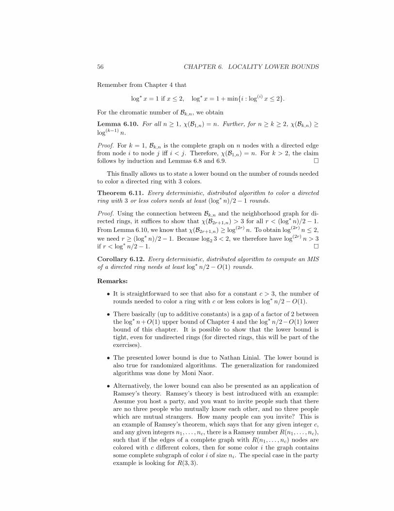
56 CHAPTER 6. LOCALITY LOWER BOUNDS
Remember from Chapter 4 that
log∗ x = 1 if x ≤ 2, log∗ x = 1 + mini : log(i) x ≤ 2.
For the chromatic number of Bk,n, we obtain
Lemma 6.10. For all n ≥ 1, χ(B1,n) = n. Further, for n ≥ k ≥ 2, χ(Bk,n) ≥log(k−1) n.
Proof. For k = 1, Bk,n is the complete graph on n nodes with a directed edgefrom node i to node j iff i < j. Therefore, χ(B1,n) = n. For k > 2, the claimfollows by induction and Lemmas 6.8 and 6.9.
This finally allows us to state a lower bound on the number of rounds neededto color a directed ring with 3 colors.
Theorem 6.11. Every deterministic, distributed algorithm to color a directedring with 3 or less colors needs at least (log∗ n)/2− 1 rounds.
Proof. Using the connection between Bk,n and the neighborhood graph for di-rected rings, it suffices to show that χ(B2r+1,n) > 3 for all r < (log∗ n)/2 − 1.From Lemma 6.10, we know that χ(B2r+1,n) ≥ log(2r) n. To obtain log(2r) n ≤ 2,we need r ≥ (log∗ n)/2− 1. Because log2 3 < 2, we therefore have log(2r) n > 3if r < log∗ n/2− 1.
Corollary 6.12. Every deterministic, distributed algorithm to compute an MISof a directed ring needs at least log∗ n/2−O(1) rounds.
Remarks:
• It is straightforward to see that also for a constant c > 3, the number ofrounds needed to color a ring with c or less colors is log∗ n/2−O(1).
• There basically (up to additive constants) is a gap of a factor of 2 betweenthe log∗ n+O(1) upper bound of Chapter 4 and the log∗ n/2−O(1) lowerbound of this chapter. It is possible to show that the lower bound istight, even for undirected rings (for directed rings, this will be part of theexercises).
• The presented lower bound is due to Nathan Linial. The lower bound isalso true for randomized algorithms. The generalization for randomizedalgorithms was done by Moni Naor.
• Alternatively, the lower bound can also be presented as an application ofRamsey’s theory. Ramsey’s theory is best introduced with an example:Assume you host a party, and you want to invite people such that thereare no three people who mutually know each other, and no three peoplewhich are mutual strangers. How many people can you invite? This isan example of Ramsey’s theorem, which says that for any given integer c,and any given integers n1, . . . , nc, there is a Ramsey number R(n1, . . . , nc),such that if the edges of a complete graph with R(n1, . . . , nc) nodes arecolored with c different colors, then for some color i the graph containssome complete subgraph of color i of size ni. The special case in the partyexample is looking for R(3, 3).

6.2. THE NEIGHBORHOOD GRAPH 57
• Ramsey theory is more general, as it deals with hyperedges. A normaledge is essentially a subset of two nodes; a hyperedge is a subset of knodes. The party example can be explained in this context: We have(hyper)edges of the form i, j, with 1 ≤ i, j ≤ n. Choosing n sufficientlylarge, coloring the edges with two colors must exhibit a set S of 3 edgesi, j ⊂ v1, v2, v3, such that all edges in S have the same color. To proveour coloring lower bound using Ramsey theory, we form all hyperedges ofsize k = 2r+1, and color them with 3 colors. Choosing n sufficiently large,there must be a set S = v1, . . . , vk+1 of k + 1 identifiers, such that allk + 1 hyperedges consisting of k nodes from S have the same color. Notethat both v1, . . . , vk and v2, . . . , vk+1 are in the set S, hence there willbe two neighboring views with the same color. Ramsey theory shows thatin this case n will grow as a power tower (tetration) in k. Thus, if n is solarge that k is smaller than some function growing like log∗ n, the coloringalgorithm cannot be correct.
• The neighborhood graph concept can be used more generally to studydistributed graph coloring. It can for instance be used to show that witha single round (every node sends its identifier to all neighbors) it is possibleto color a graph with (1 + o(1))∆2 ln n colors, and that every one-roundalgorithm needs at least Ω(∆2/ log2 ∆ + log log n) colors.
• One may also extend the proof to other problems, for instance one mayshow that a constant approximation of the minimum dominating set prob-lem on unit disk graphs costs at least log-star time.
• Using r-hop views and the fact that nodes with equal r-hop views have tomake the same decisions is the basic principle behind almost all localitylower bounds (in fact, we are not aware of a locality lower bound that doesnot use this principle). Using this basic technique (but a completely dif-ferent proof otherwise), it is for instance possible to show that computingan MIS (and many other problems) in a general graph requires at leastΩ(
√log n/ log log n) and Ω(log ∆/ log log ∆) rounds.

58 CHAPTER 6. LOCALITY LOWER BOUNDS

Chapter 7
Social Networks
Distributed computing is applicable in various contexts. This lecture exemplar-ily studies one of these contexts, social networks, an area of study whose originsdate back a century. To give you a first impression, consider Figure 7.1.
inst2
34
5
6
7
8
9
10
11
12
13
14
1516
1718
19
20
21
22
23
24
25
26
27
28
29
30
31
32
33
admin
Figure 7.1: This graph shows the social relations between the members of akarate club, studied by anthropologist Wayne Zachary in the 1970s. Two people(nodes) stand out, the instructor and the administrator of the club, both happento have many friends among club members. At some point, a dispute causedthe club to split into two. Can you predict how the club partitioned? (If not,just search the Internet for Zachary and Karate.)
59

60 CHAPTER 7. SOCIAL NETWORKS
7.1 Small-World Networks
Back in 1929, Frigyes Karinthy published a volume of short stories that pos-tulated that the world was “shrinking” because human beings were connectedmore and more. Some claim that he was inspired by radio network pioneerGuglielmo Marconi’s 1909 Nobel Prize speech. Despite physical distance, thegrowing density of human “networks” renders the actual social distance smallerand smaller. As a result, it is believed that any two individuals can be connectedthrough at most five (or so) acquaintances, i.e., within six hops.
• The topic was hot in the 1960s. For instance, in 1964, Marshall McLuhancoined the metaphor “Global Village”. He wrote: “As electrically con-tracted, the globe is no more than a village”. He argues that due to thealmost instantaneous reaction times of new (“electric”) technologies, eachindividual inevitably feels the consequences of his actions and thus auto-matically deeply participates in the global society. McLuhan understoodwhat we now can directly observe – real and virtual world are moving to-gether. He realized that the transmission medium, rather than the trans-mitted information is at the core of change, as expressed by his famousphrase “the medium is the message”.
• This idea has been followed ardently in the 1960s by several sociologists,first by Michael Gurevich, later by Stanley Milgram. Milgram wanted toknow the average path length between two “random” humans, by usingvarious experiments, generally using randomly chosen individuals fromthe US Midwest as starting points, and a stockbroker living in a suburbof Boston as target. The starting points were given name, address, oc-cupation, plus some personal information about the target. They wereasked to send a letter to the target. However, they were not allowed todirectly send the letter, rather, they had to pass it to somebody they knewon first-name basis and that they thought to have a higher probability toknow the target person. This process was repeated, until somebody knewthe target person, and could deliver the letter. Shortly after starting theexperiment, letters have been received. Most letters were lost during theprocess, but if they arrived, the average path length was about 5.5. Theobservation that the entire population is connected by short acquaintancechains got later popularized by the terms “six degrees of separation” and“small world”.
• Statisticians tried to explain Milgram’s experiments, by essentially giv-ing network models that allowed for short diameters, i.e., each node isconnected to each other node by only a few hops. Until today there is athriving research community in statistical physics that tries to understandnetwork properties that allow for “small world” effects.
• One of the keywords in this area are power-law graphs, networks werenode degrees are distributed according to a power-law distribution, i.e.the number of nodes with degree δ is proportional to δ−α, for some α > 1.Such power-law graphs have been witnessed in many application areas,apart from social networks also in the web, or in Biology or Physics.

7.1. SMALL-WORLD NETWORKS 61
• Obviously, two power-law graphs might look and behave completely dif-ferently, even if α and the number of edges is exactly the same.
One well-known model towards this end is the Watts-Strogatz model. Wattsand Strogatz argued that social networks should be modeled by a combination oftwo networks: As the basis we take a network that has a large cluster coefficient. . .
Definition 7.1. The cluster coefficient of a network is defined by the probabilitythat two friends of a node are likely to be friends as well, summing up over allthe nodes.
. . . , then we augment such a graph with random links, every node for in-stance points to a constant number of other nodes, chosen uniformly at random.This augmentation represents acquaintances that connect nodes to parts of thenetwork that would otherwise be far away.
Remarks:
• Without further information, knowing the cluster coefficient is of ques-tionable value: Assume we arrange the nodes in a grid. Technically, ifwe connect each node to its four closest neighbors, the graph has clustercoefficient 0, since there are no triangles; if we instead connect each nodewith its eight closest neighbors, the cluster coefficient is 3/7. The clus-ter coefficient is quite different, even though both networks have similarcharacteristics.
This is interesting, but not enough to really understand what is going on. ForMilgram’s experiments to work, it is not sufficient to connect the nodes in acertain way. In addition, the nodes themselves need to know how to forwarda message to one of their neighbors, even though they cannot know whetherthat neighbor is really closer to the target. In other words, nodes are notjust following physical laws, but they make decisions themselves. In contrastto those mathematicians that worked on the problem earlier, Jon Kleinbergunderstood that Milgram’s experiment essentially shows that social networksare “navigable”, and that one can only explain it in terms of a greedy routing.
In particular, Kleinberg set up an artificial network with nodes on a gridtopology, plus some additional random links per node. In a quantitative studyhe showed that the random links need a specific distance distribution to allowfor efficient greedy routing. This distribution marks the sweet spot for anynavigable network.
Definition 7.2 (Augmented Grid). We take n = m2 nodes (i, j) ∈ V =1, . . . , m2 that are identified with the lattice points on an m × m grid. Wedefine the distance between two nodes (i, j) and (k, `) as d
((i, j), (k, `)
)=
|k − i| + |` − j| as the distance between them on the m × m lattice. The net-work is modeled using a parameter α ≥ 0. Each node u has a directed edge toevery lattice neighbor. These are the local contacts of a node. In addition, eachnode also has an additional random link (the long-range contact). For all uand v, the long-range contact of u points to node v with probability proportionalto d(u, v)−α, i.e., with probability d(u, v)−α/
∑w∈V \u d(u,w)−α. Figure 7.2
illustrates the model.

62 CHAPTER 7. SOCIAL NETWORKS
Figure 7.2: Augmented grid with m = 6
Remarks:
• The network model has the following geographic interpretation: nodes(individuals) live on a grid and know their neighbors on the grid. Further,each node has some additional acquaintances throughout the network.
• The parameter α controls how the additional neighbors are distributedacross the grid. If α = 0, long-range contacts are chosen uniformly atrandom (as in the Watts-Strogatz model). As α increases, long-rangecontacts become shorter on average. In the extreme case, if α → ∞, alllong-range contacts are to immediate neighbors on the grid.
• It can be shown that as long as α ≤ 2, the diameter of the resultinggraph is polylogarithmic in n (polynomial in log n) with high probability.In particular, if the long-range contacts are chosen uniformly at random(α = 0), the diameter is O(log n).
Since the augmented grid contains random links, we do not know anythingfor sure about how the random links are distributed. In theory, all links couldpoint to the same node! However, this is almost certainly not the case. Formallythis is captured by the term with high probability.
Definition 7.3 (With High Probability). Some probabilistic event is said tooccur with high probability (w.h.p.), if it happens with a probability p ≥ 1 −1/nc, where c is a constant. The constant c may be chosen arbitrarily, but it isconsidered constant with respect to Big-O notation.
7.1. SMALL-WORLD NETWORKS 63
Remarks:
• For instance, a running time bound of c log n or ec! log n + 5000c withprobability at least 1−1/nc would be O(log n) w.h.p., but a running timeof nc would not be O(n) w.h.p. since c might also be 50.
• This definition is very powerful, as any polynomial (in n) number of state-ments that hold w.h.p. also holds w.h.p. at the same time, regardless ofany dependencies between random variables!
Theorem 7.4. The diameter of the augmented grid with α = 0 is O(log n) withhigh probability.
Proof Sketch. For simplicity, we will only show that we can reach a node wstarting from some node v. However, it can be shown that (essentially) eachof the intermediate claims holds with high probability, which then by meansof the union bound yields that all of the claims hold simultaneously with highprobability for all pairs of nodes.
Let Ng be the dlog ne-hop neighborhood of v on the grid, containing Ω(log2 n)nodes. Each of the nodes in Ng has a random link, probably leading to distantparts of the graph. As long as we have reached only o(n) nodes, any newrandom link will with probability 1− o(1) lead to a node for which none of itsgrid neighbors has been visited yet. Thus, in expectation we find almost |Ng|new nodes whose neighbors are “fresh”. Using their grid links, we will reach(4−o(1))|Ng| more nodes within one more hop. If bad luck strikes, it could stillhappen that many of these links lead to a few nodes, already visited nodes, ornodes that are very close to each other. But that is very unlikely, as we havelots of random choices! Indeed, it can be shown that not only in expectation,but with high probability (5− o(1))|Ng| many nodes are reached this way.
Because all these shiny new nodes have (so far unused) random links, wecan repeat this reasoning inductively, implying that the number of nodes growsby (at least) a constant factor for every two hops. Thus, after O(log n) hops,we will have reached n/ log n nodes (which is still small compared to n). Fi-nally, consider the expected number of links from these nodes that enter the(log n)-neighborhood of some target node w with respect to the grid. Since thisneighborhood consists of Ω(log2 n) nodes, in expectation Ω(log n) links comeclose enough to w. This is large enough to almost guarantee that this happens.Summing everything up, we still used merely O(log n) hops in total to get fromv to w.
This shows that for α = 0 (and in fact for all α ≤ 2), the resulting networkhas a small diameter. Recall however that we also wanted the network to benavigable. For this, we consider a simple greedy routing strategy (Algorithm 21).
Algorithm 21 Greedy Routing1: while not at destination do2: go to a neighbor which is closest to destination (considering grid distance
only)3: end while

64 CHAPTER 7. SOCIAL NETWORKS
Lemma 7.5. In the augmented grid, Algorithm 21 finds a routing path of lengthat most 2(m− 1) ∈ O(
√n).
Proof. Because of the grid links, there is always a neighbor which is closer tothe destination. Since with each hop we reduce the distance to the target atleast by one in one of the two grid dimensions, we will reach the destinationwithin 2(m− 1) steps.
This is not really what Milgram’s experiment promises. We want to knowhow much the additional random links speed up the process. To this end, wefirst need to understand how likely it is that two nodes u and v are connectedby a random link in terms of n and their distance d(u, v).
Lemma 7.6. Node u’s random link leads to a node v with probability
• Θ(1/(d(u, v)αm2−α)) if α < 2.
• Θ(1/(d(u, v)2 log n)) if α = 2,
• Θ(1/d(u, v)α) if α > 2.
Moreover, if α > 2, the probability to see a link of length at least d is inΘ(1/dα−2).
Proof. For α 6= 2, we have that
∑
w∈V \u
1d(u, w)α
∈m∑
r=1
Θ(r)rα
= Θ(∫ m
r=1
1rα−1
dr
)= Θ
([r2−α
2− α
]m
1
).
If α < 2, this gives Θ(m2−α), if α > 2, it is in Θ(1). If α = 2, we get
∑
w∈V \u
1d(u, w)α
∈m∑
r=1
Θ(r)r2
= Θ(1) ·m∑
r=1
1r
= Θ(log m) = Θ(log n).
Multiplying with d(u, v)α yields the first three bounds.For the last statement, compute
∑
w∈Vd(u,v)≥d
Θ(1/d(u, v)α) = Θ(∫ m
r=d
r
rαdr
)= Θ
([r2−α
2− α
]m
d
)= Θ(1/dα−2).
Remarks:
• For α 6= 2, this is bad news for the greedy routing algorithm, as it willtake nΩ(1) = mΩ(1) expected steps to reach the destination. This is dis-appointing, we were hoping for something polylogarithmic.
• If α < 2, in distance m(2−α)/3 to the target are m2(2−α)/3 many nodes.Thus it takes Θ(m(2−α)/3) links in expectation to find a link that comesthat close to the destination. Without finding such a link, we have to goat least this far using grid links only.
7.1. SMALL-WORLD NETWORKS 65
• If α > 2, it takes Θ(m(α−2)/(α−1)) steps until we see a link of lengthat least m1/(α−1) in expectation. Without such links, it takes at leastm/m1/(α−1) = m(α−2)/(α−1) steps to travel a distance of m.
• Any algorithm that uses only the information on long-range contacts thatit can collect at the so far visited nodes cannot be faster.
• However, the case α = 2 looks more promising.
Definition 7.7 (Phase). Consider routing from a node u to a node v andassume that we are at some intermediate node w. We say that we are in phasej at node w if the lattice distance d(w, v) to the target node v is between 2j <d(w, v) ≤ 2j+1.
Remarks:
• Enumerating the phases in decreasing order is useful, as notation becomesless cumbersome.
• There are dlog me ∈ O(log n) phases.
Lemma 7.8. Assume that we are in phase j at node w when routing from u tov. The probability for getting to phase j − 1 in one step is at least Ω(1/ log n).
Proof. Let Bj be the set of nodes x with d(x, v) ≤ 2j . We get from phase jto phase j − 1 if the long-range contact of node w points to some node in Bj .Note that we always make progress while following the greedy routing path.Therefore, we have not seen node w before and the long-range contact of wpoints to a random node that is independent of anything seen on the path fromu to w.
For all nodes x ∈ Bj , we have d(w, x) ≤ d(w, v)+d(x, v) ≤ 2j+1 +2j < 2j+2.Hence, for each node x ∈ Bj , the probability that the long-range contact of wpoints to x is Ω(1/22j+4 log n). Further, the number of nodes in Bj is at least(2j)2/2 = 22j−1. Hence, the probability that some node in Bj is the long rangecontact of w is at least
Ω(|Bj | · 1
22j+4 log n
)= Ω
(22j−1
22j+4 log n
)= Ω
(1
log n
).
Theorem 7.9. Consider the greedy routing path from a node u to a node v onan augmented grid with parameter α = 2. The expected length of the path isO(log2 n).
Proof. We already observed that the total number of phases is O(log n) (thedistance to the target is halved when we go from phase j to phase j − 1). Ateach point during the routing process, the probability of proceeding to the nextphase is at least Ω(1/ log n). Let Xj be the number of steps in phase j. Becausethe probability for ending the phase is Ω(1/ log n) in each step, in expectationwe need O(log n) steps to proceed to the next phase, i.e., E[Xj ] ∈ O(log n). LetX =
∑j Xj be the total number of steps of the routing process. By linearity of
expectation, we have
E[X] =∑
j
E[Xj ] ∈ O(log2 n).

66 CHAPTER 7. SOCIAL NETWORKS
7.2 Propagation Studies
In networks, nodes may influence each other’s behavior and decisions. There aremany applications where nodes influence their neighbors, e.g. they may impacttheir opinions, or they may bias what products they buy, or they may pass ona disease.
On a beach (modeled as a line segment), it is best to place an ice creamstand right in the middle of the segment, because you will be able to “control”the beach most easily. What about the second stand, where should it settle?The answer generally depends on the model, but assuming that people will buyice cream from the stand that is closer, it should go right next to the first stand.
Rumors can spread astoundingly fast through social networks. Tradition-ally this happens by word of mouth, but with the emergence of the Internetand its possibilities new ways of rumor propagation are available. People writeemail, use instant messengers or publish their thoughts in a blog. Many factorsinfluence the dissemination of rumors. It is especially important where in a net-work a rumor is initiated and how convincing it is. Furthermore the underlyingnetwork structure decides how fast the information can spread and how manypeople are reached. More generally, we can speak of diffusion of information innetworks. The analysis of these diffusion processes can be useful for viral mar-keting, e.g. to target a few influential people to initiate marketing campaigns.A company may wish to distribute the rumor of a new product via the mostinfluential individuals in popular social networks such as Facebook. A secondcompany might want to introduce a competing product and has hence to selectwhere to seed the information to be disseminated. Rumor spreading is quitesimilar to our ice cream stand problem.
More formally, we may study propagation problems in graphs. Given agraph, and two players. Let the first player choose a seed node u1; afterwardslet the second player choose a seed node u2, with u2 6= u1. The goal of the gameis to maximize the number of nodes that are closer to one’s own seed node.
In many graphs it is an advantage to choose first. In a star graph for instancethe first player can choose the center node of the star, controlling all but onenode. In some other graphs, the second player can at least score even. But isthere a graph where the second player has an advantage?
Theorem 7.10. In a two player rumor game where both players select one nodeto initiate their rumor in the graph, the first player does not always win.
Proof. See Figure 7.3 for an example where the second player will always win,regardless of the decision the first player. If the first player chooses the node x0
in the center, the second player can select x1. Choice x1 will be outwitted by x2,and x2 itself can be answered by z1. All other strategies are either symmetric,or even less promising for the first player.

7.2. PROPAGATION STUDIES 67
x1x2
y2
y1
z1
x0
y2
z2
Figure 7.3: Counter example.