theory of computation class notes fall 2002main/theory.pdftheory of computation class notes fall...
TRANSCRIPT

Theory of ComputationClass Notes
Fall 2002
Karl WinklmannCarolyn J. C. Schauble
Department of Computer ScienceUniversity of Colorado at Boulder
September 24, 2002
c©2002 Karl Winklmann, Carolyn J. C. Schauble

2
3
Preface
Unlike most textbooks on theory of computation these notes try to build as What is differentmuch as possible on knowledge that juniors or seniors in computer science tendto have. For example, the introduction of undecidability issues in the first chap-ter starts with examples of programs that read and process other programs thatare familiar to the students: Unix utilities like grep, cat, or diff. As anotherexample, the proof of Cook’s Theorem (NP-completeness of Boolean satisfiabil-ity) [Coo71] is done in terms of “compilation”: instead of the usual approach ofturning a nondeterministic Turing machine into a Boolean expression, we com-pile a nondeterministic C++ program into machine language, and the resulting“circuit satisfiability” problem into the problem of determining satisfiability ofBoolean expressions.
All material is presented without unnecessary notational clutter. To getto strong results quickly, the text starts with the “machine model” studentsalready know as plain “programs.”
When a proof requires a substantial new concept, the concept is first pre-sented in isolation. For example, before we prove that all problems in P canbe transformed into Sat, we show transformations for a few concrete exam-ples. This allows the students to understand the concept of transformation intoBoolean expressions before we present the generic argument that covers a wholeclass of such transformations. Pedagogically this makes sense even though theexamples get superseded quickly by the more general result.
Students should know the basic concepts from a course on algorithms, including Prerequisitesthe different types of algorithms (greedy, divide-and-conquer, etc.) and theyshould have some understanding of algorithm design and analysis and of basicconcepts of discrete mathematics such as relations, functions, and Boolean op-erations. Introductions to such concepts can of course be found in many books,e.g., [Sch96] or [Dea96].
These notes are not meant for self-study. The concepts are often too subtle, Don’t try this at homeand these notes are generally too terse for that. They are meant to be read bystudents in conjunction with classroom discussion.
Karl WinklmannCarolyn Schauble
Boulder, August 5, 2002

4

Contents
1 Computability 71.1 Strings, Properties, Programs . . . . . . . . . . . . . . . . . . . . 71.2 A Proof By Contradiction . . . . . . . . . . . . . . . . . . . . . . 111.3 A Proof of Undecidability . . . . . . . . . . . . . . . . . . . . . . 121.4 Diagonalization . . . . . . . . . . . . . . . . . . . . . . . . . . . . 131.5 Transformations . . . . . . . . . . . . . . . . . . . . . . . . . . . 151.6 The Undecidability of All I/0-Properties . . . . . . . . . . . . . . 211.7 The Unsolvability of the Halting Problem . . . . . . . . . . . . . 251.8 Godel’s Incompleteness Theorem . . . . . . . . . . . . . . . . . . 25
2 Finite-State Machines 312.1 State Transition Diagrams . . . . . . . . . . . . . . . . . . . . . . 312.2 The Myhill-Nerode Theorem . . . . . . . . . . . . . . . . . . . . 412.3 The Pumping Lemma for Regular Languages . . . . . . . . . . . 62
3 Context-Free Languages 693.1 Context-Free Grammars . . . . . . . . . . . . . . . . . . . . . . . 693.2 Parsing . . . . . . . . . . . . . . . . . . . . . . . . . . . . . . . . 713.3 The Pumping Lemma for Context-Free Grammars . . . . . . . . 763.4 A Characterization of Context-Free Languages . . . . . . . . . . 84
4 Time Complexity 894.1 The State of Knowledge Before NP-Completeness . . . . . . . . . 894.2 NP . . . . . . . . . . . . . . . . . . . . . . . . . . . . . . . . . . . 934.3 The NP-completeness of Satisfiability . . . . . . . . . . . . . . 954.4 More “NP-Complete” Problems . . . . . . . . . . . . . . . . . . . 984.5 The “Holy Grail”: P = NP? . . . . . . . . . . . . . . . . . . . . . 101
Bibliography 111
5

6 CONTENTS
Chapter 1
Computability
We write programs in order to solve problems. But if a problem is ”too hard”and our program is ”too simple,” this won’t work. The sophistication of ourprogram needs to match the intrinsic difficulty of the problem.
Can this be made precise? Theory of computation attempts just that. Wewill study classes of programs, trying to characterize the classes of problemsthey solve. The approach is mathematical: we try to prove theorems.
In this first chapter we do not place any restrictions on the programs; laterwe will restrict the kinds of data structures the programs use.
Maybe surprisingly, even without any restrictions on the programs we willbe able to prove in this first chapter that many problems cannot be solved.
The central piece of mathematics in this first chapter is a proof techniquecalled “proof by contradiction.” The central piece of computer science is thenotion that the input to a program can be a program.
1.1 Strings, Properties, Programs
Programs often operate on other programs. Examples of such “tools” are edi-tors, compilers, interpreters, debuggers, utilities such as — to pick some Unixexamples — diff, lint, rcs, grep, cat, more and lots of others. Some suchprograms determine properties of programs they are operating on. For example,a compiler among other things determines whether or not the source code ofa program contains any syntax errors. Figure 1.1 shows a much more modestexample. The program “oddlength.cpp” determines whether or not its inputconsists of an odd number of characters. If we ran the program in Figure 1.1on some text file, e.g. by issuing the two commands:
CC -o oddlength oddlength.cppoddlength < phonelist
the response would be one of two words, Yes or No (assuming that the program
7

8 CHAPTER 1. COMPUTABILITY
void main( void )
{
if (oddlength())
cout << "Yes";
else
cout << "No";
}
boolean oddlength( void )
{
boolean toggle = FALSE;
while (getchar() != EOF)
{
toggle = !toggle;
}
return( toggle );
}
Figure 1.1: A program “oddlength.cpp” that determines whether or not itsinput consists of an odd number of characters
was stored in oddlength.cpp and that there was indeed a text file phonelistand that this all is taking place on a system on which these commands makesense1). We could of course run this program on the source texts of programs,even on its own source text:
CC -o oddlength oddlength.cppoddlength < oddlength.cpp
The response in this case would be No because it so happens that the sourcecode of this program consists of an even number of characters.
Mathematically speaking, writing this program was a “constructive” proofof the following theorem. To show that there was a program as claimed by thetheorem we constructed one.
Theorem 1 There is a program that outputs Yes or No depending on whetheror not its input contains an odd number of characters. (Equivalently, there isa boolean function that returns TRUE or FALSE depending on whether or not itsinput2 contains an odd number of characters.)
In theory of computation the word “decidable” is used to describe this sit-uation, as in
1For our examples of programs we assume a Unix environment and a programming languagelike C or C++. To avoid clutter we leave out the usual “#include” and “#define” statementsand assume that TRUE and FALSE have been defined to behave the way you would expect themto.
2The “input” to a function is that part of the standard input to the program that has notbeen read yet at the time the function gets called.

1.1. STRINGS, PROPERTIES, PROGRAMS 9
void main( void )
{
char c;
c = getchar();
while (c != EOF)
{
while (c == ’X’); // loop forever if an ’X’ is found
c = getchar();
}
}
Figure 1.2: A program “x.cpp” that loops on some inputs
Theorem 1 (new wording) Membership in the set LODDLENGTH = {x : |x| isodd} is decidable.
The notion of a “property” is the same as the notion of a “set”: x having Properties vs. setsproperty Π is the same as x being in the set {z : z has property Π}. Thissuggests yet another rewording of Theorem 1 which uses standard terminologyof theory of computation. If we use the name Oddlength for the property ofconsisting of an odd number of characters then the theorem reads as follows.
Theorem 1 (yet another wording) Oddlength is decidable.
Concern about whether or not a program contains an odd number of characters More interestingproperties of programsis not usually uppermost on programmers’ minds. An example of a property of
much greater concern is whether or not a program might not always terminate.Let’s say a program has property Looping if there exists an input on which theprogram will not terminate. Two examples of programs with property Loopingare shown in Figures 1.2 and 1.3. In terms of sets, having property Loopingmeans being a member of the set LLOOPING = {x : x is a syntactically correctprogram and there is an input y such that x, when run on y, will not terminate}.
Instead of being concerned with whether or not there is some input (amongthe infinitely many possible inputs) on which a given program loops, let ussimplify matters and worry about only one input per program. Let’s make thatone input the (source code of the) program itself. Let Selflooping be theproperty that a program will not terminate when run with its own source textas input. In terms of sets, Selflooping means being a member of the setLSELFLOOPING = {x : x is a syntactically correct program and, when run on x,will not terminate}.
The programs in Figures 1.2 and 1.3 both have this property. The programin Figure 1.1 does not.
The bad news about Selflooping is spelled out in the following theorem.
Theorem 2 Selflooping is not decidable.

10 CHAPTER 1. COMPUTABILITY
void main( void )
{
while (TRUE);
}
Figure 1.3: Another program, “useless.cpp,” that loops on some (in fact, all)inputs
What this means is that there is no way to write a program which will print"Yes" if the input it reads is a program that has the property Selflooping,and will print "No" otherwise. Surprising, maybe, but true and not even veryhard to prove, as we will do a little later, in Section 1.3, which starts on page 12.
The definitions of Looping and Selflooping use the notion of a “syntacticallyStrings vs. programscorrect program.” The choice of programming language does not matter forany of our discussions. Our results are not about peculiarities of somebody’sfavorite programming language, they are about fundamental aspects of any formof computation. In fact, to mention syntax at all is a red herring. We could doall our programming in a language, let’s call it C−−, in which every string is aprogram. If the string is a C or C++ program, we compile it with our trustyold C or C++ compiler. If not, we compile it into the same object code as theprogram “main () {}.” Then every string is a program and “running x on y”now makes sense for any strings x and y. It means that we store the string x ina file named, say, x.cmm, and the string y in a file named, say, y, and then weuse our new C−− compiler and do
CC-- -o x x.cmmx < y
So let’s assume from now on that we are programming in “C−−,” and thusavoid having to mention “syntactically correct” all the time.
One convenient extension to this language is to regard Unix shell constructslike
grep Boulder | sort
as programs. This program can be run on some input by
cat phonebook | grep Boulder | sortgrep Boulder phonebook | sort
or by
( grep Boulder | sort ) < phonebook

1.2. A PROOF BY CONTRADICTION 11
1.2 A Proof By Contradiction
Before we prove our first undecidability result here is an example that illustratesthe technique of proving something “by contradiction.”
Proving a theorem by contradiction starts with the assumption that thetheorem is not true. From this assumption we derive something that we knowis not true. The conclusion then is that the assumption must have been false,the theorem true. The “something” that we know is not true often takes theform of “A and not A.”
Theorem 3√
2 is irrational.
(A rational number is one that is equal to the quotient of two integers. Anirrational number is one that is not rational.)
Proof (Pythagoreans, 5th century B.C.) 3 For the sake of deriving a con-tradiction, assume that
√2 is rational.
Then √2 =
p
q(1.1)
for two integers p and q which have no factors in common: they are “relativelyprime.” Squaring both sides of (1.1) yields
2 =p2
q2(1.2)
and therefore2× q2 = p2 (1.3)
This shows that p2 contains a factor of 2. But p2 cannot have a factor of 2unless p did. Therefore p itself must contain a factor of 2, which gives p2 atleast two factors of 2:
p2 = 2× 2× r (1.4)
for some integer r. Combining (1.3) and (1.4) yields
2× q2 = 2× 2× r (1.5)
which simplifies toq2 = 2× r (1.6)
which shows that q also contains a factor of 2, contradicting the fact that p andq were relatively prime.
Next we apply this proof technique to get our first undecidability result.3according to Kline, Mathematical Thought from Ancient to Modern Times, New York,
1972, pp.32-33

12 CHAPTER 1. COMPUTABILITY
void main( void )
{
if (selflooping())
; // stop, don’t loop
else
while (TRUE); // do loop forever
}
boolean selflooping( void ) // returns TRUE if the input
{ // is a program which, when
// run with its own source code
... // as input, does not terminate;
// FALSE otherwise
}
Figure 1.4: A program “diagonal.cpp” that would exist if Selflooping weredecidable
1.3 A Proof of Undecidability
Proof of Theorem 2 For the sake of deriving a contradiction, assume thatthere is a programs that decides if its input has property Selflooping. If sucha program existed we could re-write it as a function boolean selflooping()that decides whether or not its input has property Selflooping. We couldthen write the program diagonal4 shown in Figure 1.4.
Does the program in Figure 1.4 itself have property Selflooping?
Claim 1 It does not.
Proof of Claim 1 Assume it did. Then, when running the program with itsown source code as input, the function selflooping would return TRUE to themain program, making it terminate and hence not have property Selflooping,a contradiction.
Claim 2 It does.
Proof of Claim 2 Assume it did not. Then, when running the program withits own source code as input, the function selflooping would return FALSEto the main program, sending it into an infinite loop and hence have propertySelflooping, a contradiction.
These two claims form a contradiction, proving our initial assumption wrong;there cannot be a program that decides if its input has property Selflooping.
4Why diagonal is a fitting name for this program will become clear in the next section.

1.4. DIAGONALIZATION 13
digits →numbers
↓ 110
1100
1103
1104
1105
1106
1107
1108 · · ·
d = 0 . 1 1 9 1 1 9 9 9 · · ·
r1 = 0 . 6 2 8 4 1 1 0 4 · · ·r2 = 0 . 0 8 8 4 1 1 3 8 · · ·r3 = 0 . 8 4 1 1 0 8 4 1 · · ·r4 = 0 . 1 0 0 0 0 1 0 0 · · ·r5 = 0 . 0 9 9 9 9 0 9 9 · · ·r6 = 0 . 0 4 6 2 6 1 4 6 · · ·r7 = 0 . 1 1 0 0 2 1 1 0 · · ·r8 = 0 . 4 4 9 4 3 4 4 1 · · ·...
Figure 1.5: The diagonal in the proof of Theorem 4
1.4 Diagonalization
The proof of Theorem 2 was a special kind of proof by contradiction called a“diagonalization proof.” To understand that aspect of the proof, let’s look at aclassical theorem with a diagonalization proof.
Theorem 4 (Cantor, 1873) The real numbers are not countable.
(A set is countable if there is a function from the natural numbers onto theset. In other words, there is a sequence r1, r2, r3, r4, r5, . . . that contains allmembers of the set.)
Proof (Cantor, 1890/1891) 5 Assume the real numbers are countable.Then there is a sequence that contains all reals and a subsequence r1, r2,
r3, . . . that contains all reals from the interval (0, 1]. Consider the infinite matrixthat contains in row i a decimal expansion of ri, one digit per column. (SeeFigure 1.5 for an illustration.) Consider the number d whose ith digit is 9 if thematrix entry in row i and column i is 1, and whose ith digit is 1 otherwise.
The number d thus defined differs from every number in the sequence r1,r2, r3, . . ., contradicting the assumption that all reals from [0, 1) were in thesequence.6
5Cantor gave a different first proof in 1873, according to Kline, p.997.6There is a subtlety in this proof stemming from the fact that two different decimal ex-
pansions can represent the same number: 0.10000 . . . = 0.09999 . . .. Why is this of concern?And why is the proof ok anyway?
14 CHAPTER 1. COMPUTABILITY
programs (used as inputs) →programs
↓ p1 p2 p3 p4 p5 p6 p7 p8 · · ·
diagonal : 1 1 0 1 1 0 0 0 · · ·
p1 : 0 0 0 0 1 1 0 0 · · ·p2 : 0 0 0 0 1 1 0 0 · · ·p3 : 0 0 1 1 0 0 0 1 · · ·p4 : 1 0 0 0 0 1 0 0 · · ·p5 : 0 0 0 0 0 0 0 0 · · ·p6 : 0 0 0 0 0 1 0 0 · · ·p7 : 1 1 0 0 0 1 1 0 · · ·p8 : 0 0 0 0 0 0 0 1 · · ·...
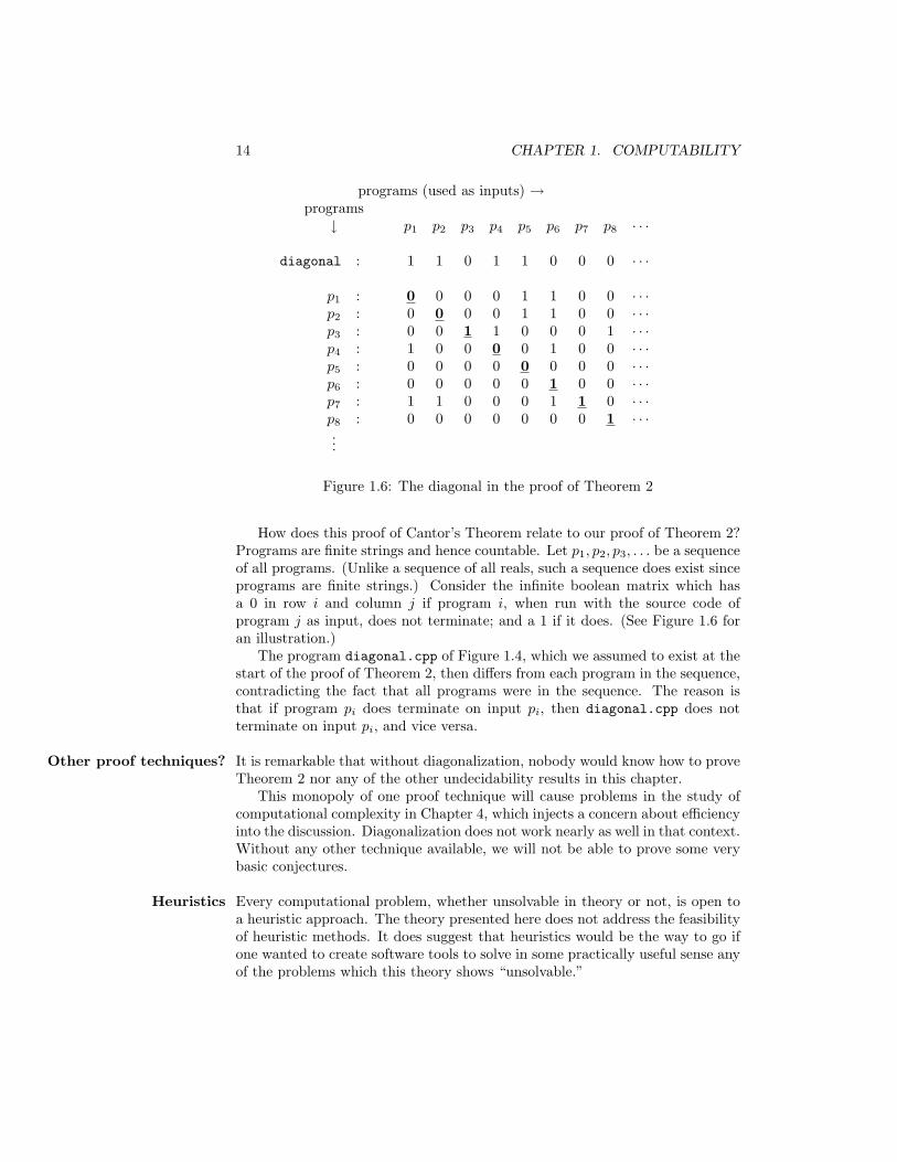
Figure 1.6: The diagonal in the proof of Theorem 2
How does this proof of Cantor’s Theorem relate to our proof of Theorem 2?Programs are finite strings and hence countable. Let p1, p2, p3, . . . be a sequenceof all programs. (Unlike a sequence of all reals, such a sequence does exist sinceprograms are finite strings.) Consider the infinite boolean matrix which hasa 0 in row i and column j if program i, when run with the source code ofprogram j as input, does not terminate; and a 1 if it does. (See Figure 1.6 foran illustration.)
The program diagonal.cpp of Figure 1.4, which we assumed to exist at thestart of the proof of Theorem 2, then differs from each program in the sequence,contradicting the fact that all programs were in the sequence. The reason isthat if program pi does terminate on input pi, then diagonal.cpp does notterminate on input pi, and vice versa.
It is remarkable that without diagonalization, nobody would know how to proveOther proof techniques?Theorem 2 nor any of the other undecidability results in this chapter.
This monopoly of one proof technique will cause problems in the study ofcomputational complexity in Chapter 4, which injects a concern about efficiencyinto the discussion. Diagonalization does not work nearly as well in that context.Without any other technique available, we will not be able to prove some verybasic conjectures.
Every computational problem, whether unsolvable in theory or not, is open toHeuristicsa heuristic approach. The theory presented here does not address the feasibilityof heuristic methods. It does suggest that heuristics would be the way to go ifone wanted to create software tools to solve in some practically useful sense anyof the problems which this theory shows “unsolvable.”

1.5. TRANSFORMATIONS 15
Digressing for a moment from our focus on what programs can and cannot do, Self-reference in otherdomainsprograms that process programs are not the only example of self-referencing
causing trouble, and far from the oldest one. Here are a few others.An example known to Greek philosophers over 2000 years ago is the self-
referencing statement that says “This statement is a lie.” This may look like apretty silly statement to consider, but it is true that the variant that says “Thisis a theorem for which there is no proof,” underlies what many regard as themost important theorem of 20th-century mathematics, Godel’s IncompletenessTheorem. More on that in Section 1.8 on page 25.
A (seemingly) non-mathematical example arises when you try to compile a“Catalog of all catalogs,” which is not a problem yet, but what about a “Catalogof all those catalogs that do not contain a reference to themselves?” Does itcontain a reference to itself? If we call catalogs that contain a reference tothemselves “self-promoting,” the trouble stems from trying to compile a “catalogof all non-self-promoting catalogs.” Note the similarity to considering a programthat halts on all those programs that are “selflooping.”
1.5 Transformations
Selflooping is not the only undecidable property of programs. To proveother properties undecidable, we will exploit the observation that they havestrong connections to Selflooping, connections such that the undecidabilityof Selflooping “rubs off” on them. Specifically, we will show that there are“transformations” of Selflooping into other problems.
Before we apply the concept of transformations to our study of(un)decidability, let’s look at some examples of transformations in other set-tings.
Consider the Unix command
sort
It can be used like
sort < phonebook
to sort the lines of a text file. “sort” solves a certain problem, called Sorting,a problem that is so common and important that whole chapters of books havebeen written about it (and a solution comes with every computer system youmight want to buy).
But what if the problem you want to solve is not Sorting, but the problemof Sorting-Those-Lines-That-Contain-the-Word-“Boulder”, stltctwbfor short? You could write a program “stltctwb” to solve stltctwb and useit like
stltctwb < phonebook

16 CHAPTER 1. COMPUTABILITY
But probably you would rather do
cat phonebook | grep Boulder | sort
This is an example of a transformation. The command “grep Boulder”transforms the stltctwb problem into the Sorting problem. The command“grep Boulder | sort” solves the stltctwb problem. (The “cat phonebook| ” merely provides the input.)
The general pattern is that if “b” is a program that solves problem B, and
a to b | b
solves problem A, then
a to b
is called a transformation of problem A into problem B.The reason for doing such transformations is that they are a way to solve
problems. If we had to formulate a theorem about the matter it would read asfollows. (Let’s make it an “Observation.” That way we don’t have to spell outa proof.)
Observation 1 If there is a program that transforms problem A into problemB and there is a program that solves problem B, then there is a program thatsolves problem A.
Since at the moment we are more interested in proving that things cannotbe done than in proving that things can be done, the following rephrasing ofthe above observation will be more useful to us.
A problem is solvable if there exists a program for solving it.
Observation 2 If there is a program that transforms problem A into problemB and problem A is unsolvable, then problem B is unsolvable as well.
In good English, “problems” get “solved” and “questions” get “decided.” Fol-“Solvable” or“decidable?” lowing this usage, we speak of “solvable and unsolvable problems” and “de-
cidable and undecidable questions.” For the substance of our discussion thisdistinction is of no consequence. For example, solving the Selflooping prob-lem for a program x is the same as deciding whether or programs have theproperty Selflooping. In either case, the prefix “un-” means that there is noprogram to do the job.
For another example of a transformation, consider the following two problems.Transforming binaryaddition into Boolean
satisfiability (Sat)Let Binary Addition be the problem of deciding, given a string like
1 0 + 1 1 = 0 1 1 (1.7)

1.5. TRANSFORMATIONS 17
whether or not it is a correct equation between binary numbers. (This oneisn’t.) Let’s restrict the problem to strings of the form
x2 x1 + y2 y1 = z3 z2 z1 (1.8)
with each xi, yi, and zi being 0 or 1. Let’s call this restricted version 2-Add.Let Boolean Satisfiability (Sat) be the problem of deciding, given a Boolean
expression, whether or not there is an assignment of truth values to the variablesin the expression which makes the whole expression true.
A transformation of 2-Add to Sat is a function t such that for all stringsα,
α represents a correct addition of two binary numbers⇔
t(α) is a satisfiable Boolean expression.
How can we construct such a transformation? Consider the Boolean circuit inFigure 1.7. It adds up two 2-bit binary numbers. Instead of drawing the picturewe can describe this circuit equally precisely by the Boolean expression
(( x1 ⊕ y1 ) ⇔ z1 ) ∧(( x1 ∧ y1 ) ⇔ c2 ) ∧(( x2 ⊕ y2 ) ⇔ z′2 ) ∧(( x2 ∧ y2 ) ⇔ c′3 ) ∧(( c2 ⊕ z′2 ) ⇔ z2 ) ∧(( c2 ∧ z′2 ) ⇔ c′′3 ) ∧(( c′3 ∨ c′′3 ) ⇔ z3 )
This suggests transformation of 2-Add to Sat that maps the string (1.7) tothe expression
(( 0 ⊕ 1 ) ⇔ 1 ) ∧(( 0 ∧ 1 ) ⇔ c2 ) ∧(( 1 ⊕ 1 ) ⇔ z′2 ) ∧(( 1 ∧ 1 ) ⇔ c′3 ) ∧(( c2 ⊕ z′2 ) ⇔ 1 ) ∧(( c2 ∧ z′2 ) ⇔ c′′3 ) ∧(( c′3 ∨ c′′3 ) ⇔ 0 )
which, appropriately, is not satisfiable. There are four variables to choose valuesfor, c2, z′2, c′3, and c′′3 , but no choice of values for them will make the wholeexpression true. Note that every single one of the seven “conjuncts” can bemade true with some assignment of truth values to c2, z′2, c′3, and c′′3 , but notall seven can be made true with one and the same assignment. In terms of thecircuit this means that if the inputs and outputs are fixed to reflect the valuesgiven in (1.7), at least one gate in the circuit has to end up with inconsistentvalues on its input and output wires, or at least one wire has to have differentvalues at its two ends. The circuit is “not satisfiable.”

18 CHAPTER 1. COMPUTABILITY
c
c’’
+
++ ^ ^
^
v
z
z
z
x y yx
z’ c’
1 21
1
22
2
3
3
3
2
Figure 1.7: A circuit for adding two 2-bit binary numbers
1.5. TRANSFORMATIONS 19
a
b
c
d
e
f
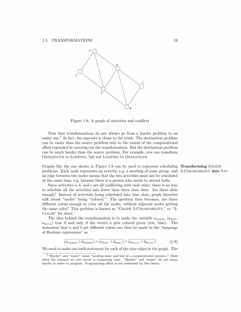
Figure 1.8: A graph of activities and conflicts
Note that transformations do not always go from a harder problem to aneasier one.7 In fact, the opposite is closer to the truth. The destination problemcan be easier than the source problem only to the extent of the computationaleffort expended in carrying out the transformation. But the destination problemcan be much harder than the source problem. For example, you can transformOddlength to Looping, but not Looping to Oddlength.
Graphs like the one shown in Figure 1.8 can be used to represent scheduling Transforming Graph3-Colorability into Satproblems. Each node represents an activity, e.g. a meeting of some group, and
an edge between two nodes means that the two activities must not be scheduledat the same time, e.g. because there is a person who needs to attend both.
Since activities a, b, and e are all conflicting with each other, there is no wayto schedule all the activities into fewer than three time slots. Are three slotsenough? Instead of activities being scheduled into time slots, graph theoriststalk about “nodes” being “colored.” The question then becomes, are threedifferent colors enough to color all the nodes, without adjacent nodes gettingthe same color? This problem is known as “Graph 3-Colorability,” or “3-Color” for short.
The idea behind the transformation is to make the variable aGREEN (aRED,aBLUE) true if and only if the vertex a gets colored green (red, blue). Thestatement that a and b get different colors can then be made in the “languageof Boolean expressions” as
(aGREEN ∧ bGREEN) ∧ (aRED ∧ bRED ) ∧ (aBLUE ∧ bBLUE ) (1.9)
We need to make one such statement for each of the nine edges in the graph. The7“Harder” and “easier” mean “needing more and less of a computational resource.” Most
often the resource we care about is computing time. “Harder” and “easier” do not meanharder or easier to program. Programming effort is not addressed by this theory.
20 CHAPTER 1. COMPUTABILITY
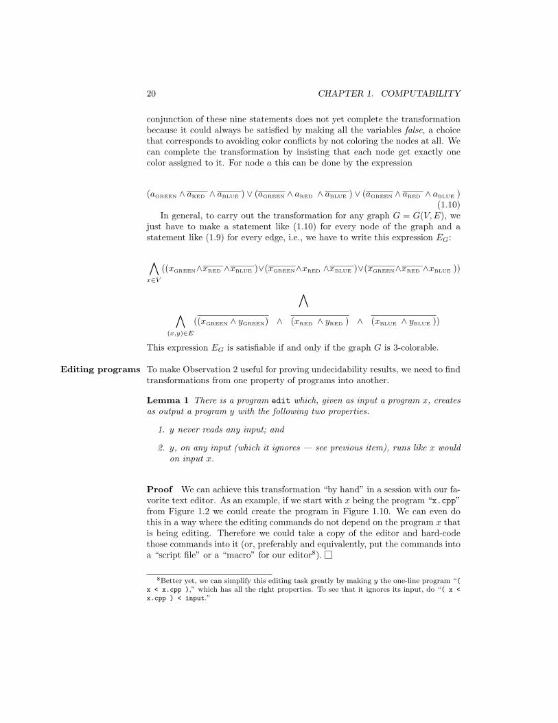
conjunction of these nine statements does not yet complete the transformationbecause it could always be satisfied by making all the variables false, a choicethat corresponds to avoiding color conflicts by not coloring the nodes at all. Wecan complete the transformation by insisting that each node get exactly onecolor assigned to it. For node a this can be done by the expression
(aGREEN ∧ aRED ∧ aBLUE ) ∨ (aGREEN ∧ aRED ∧ aBLUE ) ∨ (aGREEN ∧ aRED ∧ aBLUE )(1.10)
In general, to carry out the transformation for any graph G = G(V, E), wejust have to make a statement like (1.10) for every node of the graph and astatement like (1.9) for every edge, i.e., we have to write this expression EG:
∧
x∈V
((xGREEN∧xRED ∧xBLUE )∨(xGREEN∧xRED ∧xBLUE )∨(xGREEN∧xRED ∧xBLUE ))
∧
∧
(x,y)∈E
((xGREEN ∧ yGREEN) ∧ (xRED ∧ yRED ) ∧ (xBLUE ∧ yBLUE ))
This expression EG is satisfiable if and only if the graph G is 3-colorable.
To make Observation 2 useful for proving undecidability results, we need to findEditing programstransformations from one property of programs into another.
Lemma 1 There is a program edit which, given as input a program x, createsas output a program y with the following two properties.
1. y never reads any input; and
2. y, on any input (which it ignores — see previous item), runs like x wouldon input x.
Proof We can achieve this transformation “by hand” in a session with our fa-vorite text editor. As an example, if we start with x being the program “x.cpp”from Figure 1.2 we could create the program in Figure 1.10. We can even dothis in a way where the editing commands do not depend on the program x thatis being editing. Therefore we could take a copy of the editor and hard-codethose commands into it (or, preferably and equivalently, put the commands intoa “script file” or a “macro” for our editor8).
8Better yet, we can simplify this editing task greatly by making y the one-line program “(x < x.cpp ),” which has all the right properties. To see that it ignores its input, do “( x <
x.cpp ) < input.”

1.6. THE UNDECIDABILITY OF ALL I/0-PROPERTIES 21
void main( void )
{
x_on_x_no_input();
}
void x_on_x_no_input( void ) // runs like x, but
{ // instead of reading
... // input it ‘‘reads’’
} // from a string constant
Figure 1.9: The result of editing program x
1.6 The Undecidability of All I/0-Properties
Recall that Looping is the property that there exists an input on which theprogram will not terminate.
Theorem 5 Looping is undecidable.
Proof The program edit of Lemma 1 transforms Selflooping into Loop-ing. By Observation 2 this proves Looping undecidable.
What other properties of programs are often of interest? The prime consider-ation usually is whether or not a program “works correctly.” The exact meaningof this depends on what you wanted the program to do. If you were working onan early homework assignment in Programming 101, “working correctly” mayhave meant printing the numbers 1, 2, 3, . . . , 10.
Let One to Ten be the problem of deciding whether or not a programprints the numbers 1, 2, 3, . . . , 10.
Theorem 6 One to Ten is undecidable.
Proof Figure 1.11 illustrates a transformation of Selflooping into the nega-tion of property One to Ten.
Note that unlike the function x on x no input in the previous proof, thefunction x on x no input no output suppresses whatever output the programx might have generated when run on its own source code as input. This isnecessary because otherwise the transformation would not work in the case ofprograms x that print the numbers 1, 2, 3, . . . , 10.
Since the negation of One to Ten is undecidable, so is the property Oneto Ten.
How many more undecidability results can we derive this way?Figure 1.13 shows an example of an “input-output table” IOx of a program
x. For every input, the table shows the output that the program produces. Ifthe program loops forever on some input and keeps producing output, the entryin the right-hand column is an infinite string.

22 CHAPTER 1. COMPUTABILITY
#define EOF NULL // NULL is the proper end marker since
// we are ‘‘reading’’ from a string.
void main( void )
{
x_on_x_no_input();
}
char mygetchar( void )
{
static int i = 0;
static char* inputstring =
// start of input string //////////////////////////////
"\
\n\
void main( void )\n\
{\n\
char c;\n\
\n\
c = getchar();\n\
while (c != EOF)\n\
{\n\
while (c == ’X’); // loop forever if an ’X’ is found\n\
c = getchar();\n\
}\n\
};\n\
";
// end of input string ////////////////////////////////
return( inputstring[i++] );
}
void x_on_x_no_input( void )
{
char c;
c = mygetchar();
while (c != EOF)
{
while (c == ’X’); // loop forever if an ’X’ is found
c = mygetchar();
}
}
Figure 1.10: The result of editing the program “x.cpp” of Figure 1.2

1.6. THE UNDECIDABILITY OF ALL I/0-PROPERTIES 23
void main( void )
{
x_on_x_no_input_no_output();
one_to_ten();
}
void x_on_x_no_input_no_output( void )
{ // runs like x, but
// instead of reading
... // input it ‘‘reads’’
// from a string constant,
// and it does not
} // generate any output
void one_to_ten( void )
{
int i;
for (i = 1; i <= 10; i++)
cout << i << endl;
}
Figure 1.11: Illustrating the proof of Theorem 6
void main( void )
{
x_on_x_no_input_no_output();
notPI();
}
void x_on_x_no_input_no_output( void )
{
...
}
void notPI( void ) // runs like a program
{ // that does not have
... // property PI
}
Figure 1.12: The result of the editing step rice on input x

24 CHAPTER 1. COMPUTABILITY
Inputs Outputsλ Empty input file.0 Okay.100 Yes.01 Yes. Yes. Yes. ...10 No.11000 Yes. No. Yes. No. Yes. No. · · ·001 Segmentation fault.010 Core dumped....
...
Figure 1.13: The “input-output function” of a lousy program
These tables are not anything we would want to store nor do we want to“compute” them in any sense. They merely serve to define what an “input-output property” is. Informally speaking, a property of programs is an input-output property if the information that is necessary to determine whether or nota program x has the property is always present in the program’s input-outputtable IOx. For example, the property of making a recursive function call on someinput, let’s call it Recursive, is not an input-output property. Even if you knewthe whole input-output table such as the one in Figure 1.13, you would still notknow whether the program was recursive. The property of running in linear timeis not an input-output property, nor is the property of always producing someoutput within execution of the first one million statements, nor the property ofbeing a syntactically correct C program. Examples of input-output propertiesinclude
• the property of generating the same output for all inputs,
• the property of not looping on any inputs of length less that 1000,
• the property of printing the words Core dumped on some input.
More formally, a property Π of programs is an input-output property if thefollowing is true:
For any two programs a and b, if IOa = IOb then either both aand b have property Π, or neither does.
A property of programs is trivial if either all programs have it, or if none do.Thus a property of programs is nontrivial if there is at least one program thathas the property and one that doesn’t.9
9There are only two trivial properties of programs. One is the property of being a program

1.7. THE UNSOLVABILITY OF THE HALTING PROBLEM 25
Theorem 7 (Rice’s Theorem) No nontrivial input-output property of pro-grams is decidable.
Proof Let Π be a nontrivial input-output property of programs. There aretwo possibilities. Either the program
main () { while (TRUE); } (1.11)
has the property Π or it doesn’t. Let’s first prove the theorem for properties Πwhich this program (1.11) does have.
Let notPI be a function that runs like a program that does not have propertyΠ. Consider the program that is outlined in Figure 1.12. It can be created fromx by a program, call it rice, much like the program in Figure 1.9 was createdfrom x by the program edit of Lemma 1.
The function rice transforms Selflooping into Π, which proves Π unde-cidable.
What if the infinite-loop program in (1.11) does not have property Π? Inthat case we prove Rice’s Theorem for the negation of Π — by the argument inthe first part of this proof — and then observe that if the negation of a propertyis undecidable, so is the property itself.
1.7 The Unsolvability of the Halting Problem
The following result is probably the best-known undecidability result.
Theorem 8 (Unsolvability of the Halting Problem) There is no programthat meets the following specification. When given two inputs, a program x and astring y, print “Yes” if x, when run on y, terminates, and print “No” otherwise.
Proof Assume Halting is decidable. I.e. assume there is a program haltingwhich takes two file names, x and y, as arguments and prints Yes if x, whenrun on y, halts, and prints No otherwise. Then Selflooping can be solved byrunning halting with the two arguments being the same, and then reversingthe answer, i.e., changing Yes to No and vice versa.
1.8 Godel’s Incompleteness Theorem
Once more digressing a bit from our focus on programs and their power, it isworth pointing out that our proof techniques easily let us prove what is certainlythe most famous theorem in mathematical logic and one of the most famous in
— all programs have that property. The other is the property of not being a program — noprogram has that property. In terms of sets, these are the set of all programs and the emptyset.

26 CHAPTER 1. COMPUTABILITY
all of mathematics. The result was published in 1931 by Kurt Godel and putan end to the notion that if only we could find the right axioms and proof rules,we could prove in principle all true conjectures. Put another way, it put an endto the notion that mathematics could somehow be perfectly “automated.”
Theorem 9 (Godel’s Incompleteness Theorem, 1931)10 For any systemof formal proofs that includes at least the usual axioms about natural numbers,there are theorems that are true but do not have a proof in that system.
Proof If every true statement had a proof, Selflooping would be decidable,by the following algorithm.
For any given program x the algorithm generates all strings in some system-atic order until it finds either a proof that x has property Selflooping or aproof that x does not have property Selflooping.
It is crucial for the above argument that verification of formal proofs can beautomated, i.e., done by a program. It is not the verification of formal proofsthat is impossible. What is impossible is the design of an axiom system that isstrong enough to provide proofs for all true conjectures.
Does this mean that once we choose a set of axioms and proof rules, ourmathematical results will forever be limited to what can be proven from thoseaxioms and rules? Not at all. The following lemma is an example.
Lemma 2 For any system of formal proofs, the program in Figure 1.14 doeshave property Selflooping but there is no formal proof of that fact within thesystem.
Proof The program in Figure 1.14 is a modification of the program we used toprove Selflooping undecidable. Now we prove Selflooping “unprovable.”When given its own source as input, the program searches systematically for aproof that it does loop and if it finds one it terminates. Thus the existence ofsuch a proof leads to a contradiction. Since no such proof exists the programkeeps looking forever and thus does in fact have property Selflooping.
Note that there is no contradiction between the fact that there is no proof ofthis program having property Selflooping within the given axiom system andthe fact that we just proved that the program has property Selflooping. Itis just that our (informal) proof cannot be formalized within the given system.
What if we enlarged the system, for example by adding one new axiom thatsays that this program has property Selflooping? Then we could prove thatfact (with a one-line proof no less). This is correct but note that the programhad the axiom system “hard coded” in it. So if we change the system we get anew program and the lemma is again true — for the new program.
10Kurt Godel, Uber formal unentscheidbare Satze der Principia Mathematica und ver-wandter Systeme I, Monatshefte fur Mathematik und Physik, 38, 1931, 173–98.

1.8. GODEL’S INCOMPLETENESS THEOREM 27
void main( void )
{
// systematically generates all proofs
... // in the proof system under consideration
// and stops if and when it finds a proof
// that its input has property SELFLOOPING
}
Figure 1.14: Illustrating the proof of Lemma 2
Exercises
Ex. 1.1. The rational numbers are countable (as argued in class). Why does Diagonalizationthe diagonalization proof that shows that the real numbers are not countablenot work for the rational numbers?
Ex. 1.2. Is it decidable if a program has a “memory leak?”
Ex. 1.3. Is it decidable if a program will try to “de-reference a null pointer?”
Ex. 1.4. Let Selfrecursive be the property of programs that they makea recursive function call when running on their own source code as input. De-scribe a diagonalization proof that Selfrecursive is not decidable.
Ex. 1.5. Somebody who has not taken this course cannot believe that thereis no way to write a program that finds out, given a program p and input x,whether or not p when run on input x goes into an infinite loop. That personhands you a floppy with the source code of a program that they claim does infact carry out that analysis.
Can you produce a program p and input x on which their program fails?
Ex. 1.6. Describe a transformation from Selflooping to the property of Transformationsnot reading any input.
Ex. 1.7. The function edit that is used in the proof of Theorem 5 transformsSelflooping not only to Looping but also to other properties. Give threesuch properties.
Ex. 1.8. Consider the following problem. Given a graph, is there a set of edgesso that each node is an endpoint of exactly one of the edges in that set. (Sucha set of edges is called a ”complete matching”.) Describe a transformation ofthis problem to the satisfiability problem for Boolean expressions. You may dothis by showing (and explaining, if it’s complicated) the expression for one ofthe above graphs.

28 CHAPTER 1. COMPUTABILITY
Ex. 1.9. If G is a graph that you are trying to find a 3-coloring for, if t(G) isthe Boolean expression the graph gets translated into by our transformation of3-Color into Sat, and, finally, if someone handed you an assignment of truthvalues to the variables of t(G) that satisfied the expression, describe how youcan translate that assignment of truth values back to a 3-coloring of the graph.
Ex. 1.10. Consider trying to transform 3-Color into Sat but using, in placeof
(aGREEN ∧ aRED ∧ aBLUE ) ∨ (aGREEN ∧ aRED ∧ aBLUE ) ∨ (aGREEN ∧ aRED ∧ aBLUE )
the expressionxGREEN ∨ xRED ∨ xBLUE .
(a) Would this still be a transformation of 3-Color into Sat? Explain why,or why not.
(b) Could we still translate a satisfying assignment of truth values back intoa 3-coloring of the graph? Explain how, or why not.
Ex. 1.11. (a) Transform Selflooping into the property of halting on thoseinputs that contain the word Halt, and looping on all others. (b) What doesthis prove?
Ex. 1.12. (a) Transform Oddlength into Selflooping. (b) What does thisprove?
Ex. 1.13. Give three undecidable properties of programs that are not input-I/0-Propertiesoutput properties and that were not mentioned in the notes. Give three othersthat are nontrivial I/O properties, hence undecidable, but were not mentionedin class.
Ex. 1.14. We needed to suppress the output in the x on x no input no outputfunction used in the proof of Rice’s Theorem. Which line of the proof could oth-erwise be wrong?
Ex. 1.15. Is Selflooping an input-output property?
Ex. 1.16. Formulate and prove a theorem about the impossibility of programMore UndecidabilityResults optimization.
Ex. 1.17. “Autograders” are programs that check other programs for cor-rectness. For example, an instructor in a programming course might give aprogramming assignment and announce that your programs will be graded bya program she wrote.
10If having a choice is not acceptable in a real “algorithm,” we can always program thealgorithm to prefer red over green over blue.

1.8. GODEL’S INCOMPLETENESS THEOREM 29
What does theory of computing have to say about this? Choose one of thethree answers below and elaborate in no more than two or three short sentences.
1. “Autograding” is not possible.
2. “Autograding” is possible.
3. It depends on the programming assignment.
Ex. 1.18. Which of the following five properties of programs are decidable?Which are IO-properties?
1. Containing comments.
2. Containing only correct comments.
3. Being a correct parser for C (i.e., a program which outputs ”Yes” if theinput is a syntactically correct C program, and ”No” otherwise).
4. Being a correct compiler for C (i.e., a program which, when the input is aC program, outputs an equivalent machine-language version of the input.”Equivalent” means having the same IO table.).
5. The output not depending on the input.

30 CHAPTER 1. COMPUTABILITY

Chapter 2
Finite-State Machines
In contrast to the preceding chapter, where we did not place any restrictionson the kinds of programs we were considering, in this chapter we restrict theprograms under consideration very severely. We consider only programs whosestorage requirements do not grow with their inputs. This rules out dynamicallygrowing arrays or linked structures, as well as recursion beyond a limited depth.
The central piece of mathematics for this chapter is the notion of an “equiv-alence relation.” It will allow us to arrive at a complete characterization ofwhat these restricted programs can do. Applying mathematical induction willprovide us with a second complete characterization.
2.1 State Transition Diagrams
Consider the program oddlength from Figure 1.1 on page 8. Let’s use a de- The program oddlength,once more, in a picturebugger on it and set a breakpoint just before the getchar() statement. When
the program stops for the first time at that breakpoint, we can examine thevalues of its lone variable. The value of toggle is FALSE at that time and the“instruction pointer” is of course just in front of that getchar() statement.Let’s refer to this situation as state A.
If we resume execution and provide an input character, then at the nextbreak the value of toggle will be TRUE and the instruction pointer will of courseagain be just in front of that getchar(). This is another “state” the programcan be in. Let’s call it state B.
Let’s give the program another input character. The next time our debuggerlets us look at things the program is back in state A. As long as we keep feedingit input characters, it bounces back and forth between state A and state B.
What does the program do when an EOF happens to come around? Fromstate A the program will output No, from state B Yes.
Figure 2.1 summarizes all of this, in a picture. The double circle means thatan EOF produces a Yes, the single circle, a No. Σ is the set of all possible input
31

32 CHAPTER 2. FINITE-STATE MACHINES
BA
Σ
Σ
Figure 2.1: The program oddlength as a finite-state machine
characters, the input alphabet. Labeling a transition with Σ means that anyinput character will cause that transition to be made.
A picture such as the one in Figure 2.1 describes a finite-state machine or aTerminologyfinite-state automaton. States drawn as double circles are accepting states, singlecircles are rejecting states. Input characters cause transitions between states.Arrows that go from state to state and are labeled with input characters indicatewhich input characters cause what transitions. For every state and every inputcharacter there must be an arrow starting at that state and labeled by the inputcharacter. The initial state, or start state, is indicated by an unlabeled arrow.1
An input string that makes the machine end up in an accepting (rejecting)state is said to be accepted (rejected) by the machine. If M is a finite-statemachine M then LM = {x : x is accepted by M} is the language accepted byM .
Let LMATCH be the language of all binary strings that start and end with a 0 orAnother Examplestart and end with a 1. Thus LMATCH = {0, 1, 00, 11, 000, 010, 101, 111, 0000,0010, . . .} or, more formally,
LMATCH = {c, cxc : x ∈ {0, 1}?, c ∈ {0, 1}}. (2.1)
Can we construct a finite-state machine for this language? To have a chanceto make the right decision between accepting and rejecting a string when its lastcharacter has been read, it is necessary to remember what the first characterand the last character were. How can a finite-state machine “remember” or“know” this information? The only thing a finite-state machine “knows” at anyone time is which state it is in. We need four states for the four combinationsof values for those two characters (assuming, again, that we are dealing onlywith inputs consisting entirely of 0s and 1s). None of those four states wouldbe appropriate for the machine to be in at the start, when no characters havebeen read yet. A fifth state will serve as start state.
1Purists would call the picture the “transition diagram” of the machine, and define themachine itself to be the mathematical structure that the picture represents. This structureconsists of a set of states, a function from states and input symbols to states, a start state,and a set of accepting states.

2.1. STATE TRANSITION DIAGRAMS 33
1
1
1
0
11
0
0
0
0
Figure 2.2: A finite-state machine that accepts Lmatch
Now that we know what each state means, putting in the right transitionsis straightforward. Figure 2.2 shows the finished product.
(Note that we could have arrived at the same machine by starting with theprogram match in Figure 2.3 and translating it into a finite-state machine bythe same process that we used earlier with the program oddlength.)
Consider the language LEQ-4 of all nonempty bitstrings of length 4 or less which A third examplecontain the same number of 0s as 1s. Thus LEQ-4 = {01, 10, 0011, 0101, 0110,1001, 1010, 1100}.
What does a finite-state machine need to remember about its input to handlethis language? We could make it remember exactly what the input was, up tolength 4. This results in a finite-state machine with the structure of a binary treeof depth 4. See Figure 2.4. Such a binary tree structure corresponds to a “tablelookup” in a more conventional language. It works for any finite language.
The preceding example proves
Theorem 10 Every finite language is accepted by a finite-state machine.
The finite-state machine of Figure 2.4 is not as small as it could be. For example, Minimizing Finite-StateMachinesif we “merged” the states H, P, Q, and FF — just draw a line surrounding them
and regard the enclosed area as a new single state —, we would have reduced thesize of this machine by three states (without changing the language it accepts).
Why was this merger possible? Because from any of these four states, onlyrejecting states can be reached. Being in any one of these four states, no matterwhat the rest of the input, the outcome of the computation is always the same,viz. rejecting the input string.

34 CHAPTER 2. FINITE-STATE MACHINES
void main( void )
{
if (match())
cout << "Yes";
else
cout << "No";
}
boolean match( void )
{
char first, next, last;
first = last = next = getchar();
while (next != EOF)
{
last = next;
next = getchar();
}
return ((first == last) && (first != EOF)):
}
Figure 2.3: Another “finite-state” program, match
Can J and K be merged? No, because a subsequent input 1 leads to anaccepting state from J but a rejecting state from K.
What about A and D? They both have only rejecting states as their immedi-ate successors. This is not a sufficient reason to allow a merger, though. Whatif the subsequent input is 01? Out of A the string 01 drives the machine intostate E — a fact usually written as δ(A, 01) = E — and out of D the string 01drives the machine into state δ(D, 01) = Q. One of E and Q is rejecting, theother accepting. This prevents us from merging A and D.
When is a merger of two states p and q feasible? When it is true that forall input strings s, the two states δ(p, s) and δ(q, s) are either both accepting orboth rejecting. (Note that s could be the empty string, which prevents a mergerof an accepting with a rejecting state.) This condition can be rephrased to talkabout when a merger is not feasible, viz. if there is an input string s such thatof the two states δ(p, s) and δ(q, s) one is rejecting and one is accepting. Let’scall such a string s “a reason why p and q cannot be merged.” For example, thestring 011 is a reason why states B and C in Figure 2.4 cannot be merged. Theshortest reasons for this are the strings 0 and 1. A reason why states D and Ecannot be merged is the string 11. The shortest reason for this is the emptystring.
Figure 2.5 is an illustration for the following observation, which is the basisfor an algorithm for finding all the states that can be merged.
Observation 3 If c is a character and s a string, and cs is a shortest reasonwhy p and q cannot be merged, then s is a shortest reason why δ(p, c) and δ(q, c)

2.1. STATE TRANSITION DIAGRAMS 35
A
B C
E
OLKJIH
D F G
FF
EEDDBBAA CCP Q R S T U V W X Y Z
0 0 0 0
0 0
0 0 0 0 0 0 0 01 1 1 1
0,1
. . .
NM
1 1 1
0 1
0,10,10,1
0,1
1 1 1 1
11
1
Figure 2.4: A finite-state machine for LEq-4

36 CHAPTER 2. FINITE-STATE MACHINES
p q
S S
c c
Figure 2.5: Illustrating Observation 3
cannot be merged.
Observation 3 implies that the algorithm is Figure 2.6 is correct.When carrying out this algorithms by hand, it is convenient to keep track
of clusters of states.2 Two states p and q are in the same cluster if (p, q) ∈MergablePairs. As we find reasons for not merging states, i.e., as we find thecondition of the if-statement to be true, we break up the clusters. If p and qare two states that cannot be merged and the shortest reason for that is a stringof length k > 0, then p and q will remain together through the first k− 1 passesthrough the repeat-loop and get separated in the kth pass.
For example, consider the finite-state machine in Figure 2.7. It accepts“identifiers with one subscript” such as A[2], TEMP[I], LINE1[W3], X034[1001].Figure 2.8 shows how the clusters of states develop during execution of theminimization algorithm. States a and b get separated in the third pass, which isconsistent with the fact that the shortest strings that are reasons not to mergea and b are of length 3, for example “[0].”
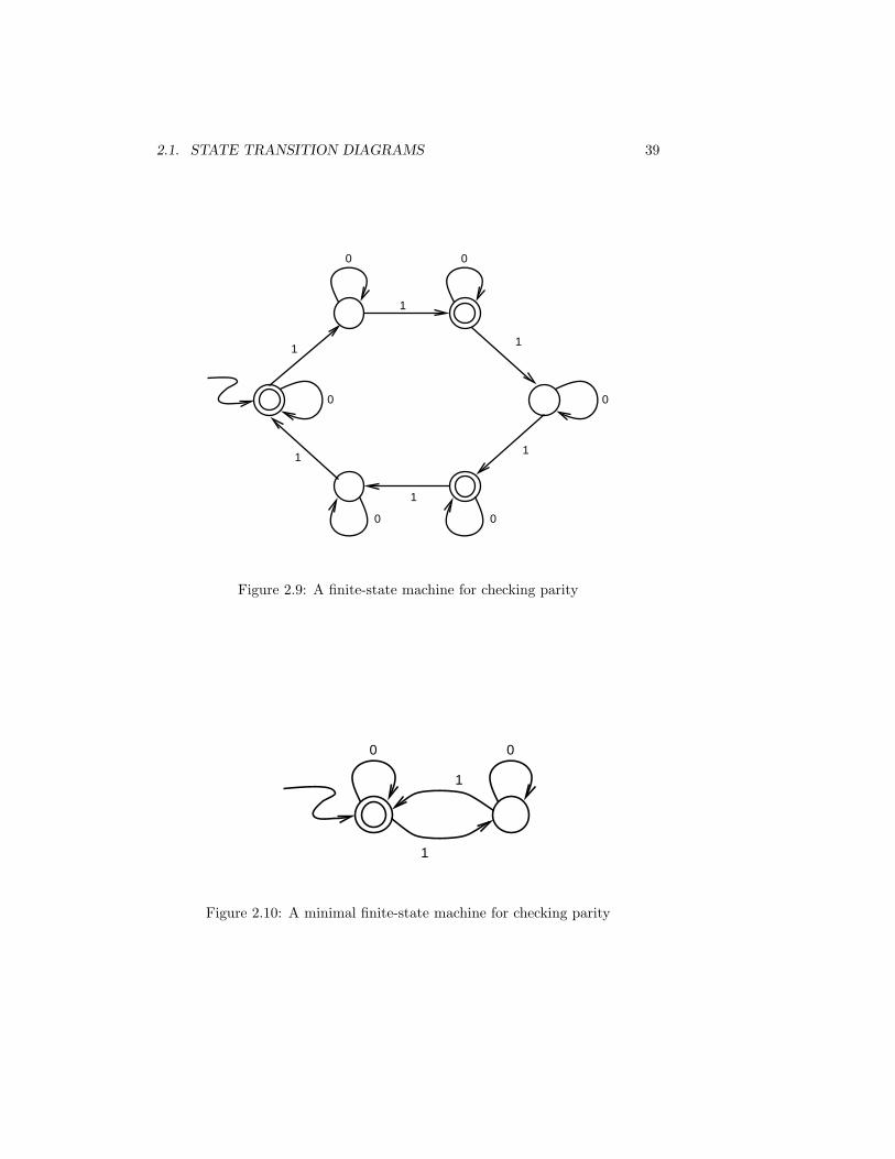
Other examples are the finite-state machines in Figures 2.9 and 2.4. On thefinite-state machine of Figure 2.9 the algorithm ends after one pass through theloop, resulting in the machine shown in Figure 2.10. The binary-tree-shapedmachine of Figure 2.4 takes three passes, resulting in the machine shown inFigure 2.11.
2Note: This works because the binary relation MergablePairs is always an equivalencerelation.

2.1. STATE TRANSITION DIAGRAMS 37
MergablePairs = ( States × States )− ( AcceptingStates × RejectingStates )
repeatOldMergablePairs = MergablePairs
for all (p, q) ∈ MergablePairsfor all input characters c
if ( (δ(p, c), δ(q, c)) 6∈ OldMergablePairs )MergablePairs = MergablePairs − (p, q)
untilMergablePairs = OldMergablePairs
Figure 2.6: An algorithm for finding all mergable states in a finite-state machine
a b c f g
d
h
Α..Ζ
Α..Ζ
Α..Ζ
0..9
0..90..9
Α..Ζ
[]]
]
]
0..9
[ [
[
] ][
[Α..Ζ
eΑ..Ζ0..9
Α..Ζ0..9[ ]
] [
0..9Α..Ζ 0..9
Figure 2.7: A finite-state machine for accepting identifiers with one subscript

38 CHAPTER 2. FINITE-STATE MACHINES
ga b c d hfe
a b c d fe h
a b he
hea
e h
Pass 1
Pass 2
Pass 3
Pass 4
che
Pass 5 (no change)
] ] ] ] ]] ]
g
g
gd
d
d
d
A A
c f
cb f
b c f ga
a b g
[ [ [ [
00000
A AA
f
Figure 2.8: Minimizing the finite-state machine of Figure 2.7
2.1. STATE TRANSITION DIAGRAMS 39
00
1
1
1
1
0
1
0
00
1
Figure 2.9: A finite-state machine for checking parity
0 0
1
1
Figure 2.10: A minimal finite-state machine for checking parity

40 CHAPTER 2. FINITE-STATE MACHINES
A
01
0 1
1 U
0,1
U 1
1
0 1
0 1
0
10
I,J,L
D
B C
G
H,O,P,Q,R,T,W,X,AA,CC,DD,EE,FF
0,1
S,U,V,Y,Z,BB
K,M,N
E,F
Figure 2.11: A minimal finite-state machine for LEq-4

2.2. THE MYHILL-NERODE THEOREM 41
quarters
nickels
dollars
pennies
dimes
halfdollars
All coins
Figure 2.12: Equivalence classes of coins
2.2 The Myhill-Nerode Theorem
Equivalence Relations, Partitions
We start with a brief introduction of equivalence relations and partitions becausethese are central to the discussion of finite-state machines.
Informally, two objects are equivalent if distinguishing between them is ofno interest. At the checkout counter of a supermarket, when you are getting 25cents back, one quarter looks as good as the next. But the difference between adime and a quarter is of interest. The set of all quarters is what mathematicianscall an “equivalence class.” The set of all dimes is another such class, as is the setof all pennies, and so on. The set of all coins gets carved up, or “partitioned,”into disjoint subsets, as illustrated in Figure 2.12. Each subset is called an“equivalence class.” Collectively, they form a “partition” of the set of all coins:every coin belongs to one and only one subset. There are finitely many suchsubsets in this example (6 to be precise).
Given a partition, there is a unique equivalence relation that goes with it: the Partitions ≡ EquivalenceRelationsrelation of belonging to the same subset.
And given an equivalence relation, there is a unique partition that goeswith it. Draw the graph of the relation. It consists of disconnected completesubgraphs whose node sets form the sets of the partition.3
3Note: This is easier to visualize when the set of nodes is finite, but works also for infinite

42 CHAPTER 2. FINITE-STATE MACHINES
All coins
penniesquarters
dollars
halfdollars
nickels
dimes
quarters1891 "D"
in mintcondition
Figure 2.13: A refinement of a partition
Just exactly what distinctions are of interest may vary. To someone who isRefinementscollecting rare coins, one quarter is not always going to look as good as thenext, but one quarter that was minted in 1891 and has a D on it and is inmint condition looks as good as the next such quarter. Our original equivalenceclass of all quarters gets subdivided, capturing the finer distinctions that are ofinterest to a coin collector. The picture of Figure 2.12 gets more boundary linesadded to it. See Figure 2.13.
What differences between program do we normally ignore? It depends on whatEquivalence RelationsAmong Programs we are interested in doing with the programs. If all we want to do is put a
printout of their source under the short leg of a wobbly table, programs withequally many pages of source code are equivalent.
A very natural notion of equivalence between programs came up in Chap-ter 1: IOa = IOb. A further refinement could take running time into account:IOa = IOb and ta = tb (“t” for time). A further refinement could in additioninclude memory usage: IOa = IOb and ta = tb and sa = sb (“s” for space).(Both t and s are functions of the input.) The refinements need not stop here.We might insist that the two programs compile to the same object code. If all wewant to do with the program is run it, we won’t care about further refinements.What else would we want to do with a program but run it? We might want tomodify it. Then two programs, one with comments and one without, are notgoing to be equivalent to us even if they are indistinguishable at run time. Sothere is a sequence of half a dozen or so successive refinements of notions of
and even uncountably infinite sets.

2.2. THE MYHILL-NERODE THEOREM 43
program equivalence, each of which is the right one for some circumstances.Next we will apply the concept of partitions and equivalence relations to
finite-state machines.
Let Parity be the set consisting of all binary strings with an even number of A Game1s. For example, 10100011 ∈ Parity, 100 6∈ Parity. Consider the followinggame, played by Bob and Alice.
1. Bob writes down a string x without showing it to Alice.
2. Alice asks a question Q about the string x. The question must be suchthat there are only finitely many different possible answers. E.g., “Whatis x?” is out, but “What are the last three digits of x?” is allowed.
3. Bob gives a truthful answer AQ(x) and writes down a string y for Aliceto see. (Alice still has not seen x.)
4. If Alice at this point has sufficient information to know whether or notxy ∈ Parity, she wins. If not, she loses.
Can Alice be sure to win this game? For example, if her question was “Whatis the last bit of x?” she might lose the game because an answer “1” and asubsequent choice of y = 1 would not allow her to know if xy ∈ Parity since xmight have been 1 or 11. What would be a better question?
Alice asks “Is the number of 1s in x even?”. She is sure to win.Tired of losing Bob suggests they play the same game with a different lan-
guage: More-0s-Than-1s, the set of bitstrings that contain more 0s than 1s.Alice asks “How many more 0s than 1s does x have?”. Bob points out that
the question is against the rules. Alice instead asks “Does x have more 0s than1s?”. Bob answers “Yes.”. Alice realizes that x could be any one of 0, 00, 000,0000, . . . and concedes defeat.
Theorem 11 Alice can’t win the More-0s-Than-1s-game.
Proof Whatever finite-answer question Q Alice asks, the answer will be thesame for some different strings among the infinite collection {0, 00, 000, 0000,. . . }. Let 0i4 and 0j be two strings such that 0 ≤ i < j and AQ(0i) = AQ(0j).The Bob can write down x = 0i or x = 0j , answer Alice’s question, and thenwrite y = 1i. Since 0i1i 6∈ More-0s-Than-1s and 0j1i ∈ More-0s-Than-1s,Alice cannot know whether or not x1i ∈ More-0s-Than-1s — she loses.
What does this game have to do with finite-state machines? It providesa complete characterization of the languages that are accepted by finite-statemachines . . .
4Note: 0i means a string consisting of i 0s.

44 CHAPTER 2. FINITE-STATE MACHINES
Theorem 12 Consider Bob and Alice playing their game with a language L.5
The following two statements are equivalent.
1. Alice can be sure to win.
2. L is accepted by some finite-state machine.
In fact, the connection between the game and finite-state machines is evenstronger.
Theorem 13 Consider Bob and Alice playing their game with the language L.The following two statements are equivalent.
1. There is a question that lets Alice win and that can always be answeredwith one of k different answers.
2. There is a finite-state machine with k states that accepts L.
To see that (2) implies (1) is the easier of the two parts of the proof. Alicedraws a picture of a k-state machine for L and asks which state the machine isin after reading x. When Bob writes down y, Alice runs M to see whether ornot it ends up in an accepting state.
The key to proving that (1) implies (2) is to understand why some questionsthat Alice might ask will make her win the game while others won’t.
Why was it that in the Parity game asking whether the last bit of x was a 1The Relation ≡L
did not ensure a win? Because there were two different choices for x, x1 = 1and x2 = 11, which draw the same answer, but for which there exists a string ywith (x1y ∈ Parity) 6⇔ (x2y ∈ Parity). In this sense the two strings x1 = 1and x2 = 11 were “not equivalent” and Alice’s question made her lose becauseit failed to distinguish between two nonequivalent strings. Such nonequivalenceof two strings is usually written as x1 6≡parity x2.
Conversely, two strings x1 and x2 are equivalent, x1 ≡parity x2, if for allstrings y, (x1y ∈ Parity) ⇔ (x2y ∈ Parity).
Definition 1 Let L be any language. Two strings x and x′ are equivalent withrespect to L, x ≡L x′, if for all strings y, (xy ∈ L) ⇔ (x′y ∈ L).
Consider the question Q that made Alice win the Divisible-by-8-game: “WhatThe Relation ≡Q
are the last three digits of x, or, if x has fewer than three digits, what is x?”.
Definition 2 Let Q be any question about strings. Two strings x and x′ areequivalent with respect to Q, x ≡Q x′, if they draw the same answer, i.e.,AQ(x) = AQ(x′).
The relation ≡Q “partitions” all strings into disjoint subset. This partition“induced by ≡Q” is illustrated in Figure 2.14.

2.2. THE MYHILL-NERODE THEOREM 45
0111,1111, ...
λ
111,
1010, ...0010,
010,
0
00000,
0000,1000,
...
101,0101,
1101, ...
011,0011,
1011,...
11
01
001,0001,
1001,...
100,0100,
1100,... 10
110,0110,
1110,...
1
Figure 2.14: The partition induced by Alice’s question
The subsets of the partition induced by ≡Q then become the state of afinite-state machine. This is illustrated in Figure 2.15. The start state is thestate containing the empty string. States containing strings in the language areaccepting states. There is a transition labeled 1 from the state that contains 0to the state that contains 01. Generally, there is a transition labeled c from thestate containing s to the state containing sc.
Could it happen that this construction results in more than one transitionwith the same label out of one state? In this example, we got lucky — Aliceasked a very nice question —, and this won’t happen. In general it might,though. As an example, Alice might have asked the question, “If x is empty,say so; if x is nonempty but contains only 0s, say so; otherwise, what are thelast three digits of x, or, if x has fewer than three digits, what is x?”. Kindof messy, but better than the original question in the sense that it takes fewerdifferent answers. The problem is that the two strings 0 and 00 draw the sameanswer, but 01 and 001 don’t. Figure 2.16 shows where this causes a problem inthe construction of a finite-state machine. The resolution is easy. We arbitrarilychoose one of the conflicting transitions and throw away the other(s). Why isthis safe? Because ≡Q is a “refinement” of ≡L and it is safe to ignore distinctionsbetween strings that are equivalent under ≡L.
It seems that the finite-state machine in Figure 2.15 is not minimal. We could The best questionrun our minimization algorithm on it, but let’s instead try to work on “mini-
5Note: A “language” in this theory means a set of strings.

46 CHAPTER 2. FINITE-STATE MACHINES
100,0100,
1100,
1
λ
11
001,0001,
1001,...
111,0111,1111,
...1
1
0
0
0
1
1
0010,010,
1010,...
...
0
0
101,0101,
1101,
0110,110,
1110,...
...
1
0
0
0
1
0
1
011 1
1
0
011,0011,
1011,...
0
0
00
0
100
1
0
0
1
000,0000,
1000,...
1
1
Figure 2.15: The finite-state machine constructed from Alice’s question
0000, ...
0, 00,
01
1001, ...001, 0001,
1
1000,
Figure 2.16: A conflict in the construction of a finite-state machine

2.2. THE MYHILL-NERODE THEOREM 47
mizing” the question Q from which the machine was constructed. Minimizinga question for us means minimizing the number of different answers.
The reason why this construction worked was that ≡Q was a refinement of≡L. This feature of the question Q we need to keep. But what is the refinementof ≡L that has the fewest subsets? ≡L itself. So the best question is “Whichsubset of the partition that is induced by ≡L does x belong to?”. This is easierto phrase in terms not of the subsets but in terms of “representative” stringsfrom the subsets: “What’s a shortest string y with x ≡L y?”.
Let’s apply this idea to the Divisible-by-8 problem. There are four equiv-alence classes:
0, 00, 000, 0000, 1000, . . . ,λ, 100, 0100, 1100, . . . ,10, 010, 110, 0010, 0110, 1010, 1110, . . . , and1, 01, 11, 001, 011, 101, 111, 0001, 0011, 0101, 0111, 1001, 1010, 1101, 1111, . . . .
The four answers to our best question are λ, 0, 10, and 1. The resulting finite-state machine has four states and is minimal.
Let’s take stock of the equivalence relations (or partitions) that play a rolein finite-state machines and the languages accepted by such machines.
As mentioned already, every language, i.e., set of strings, L defines (“induces”) The Relations ≡L, ≡Q,≡Man equivalence relation ≡L between strings:
(x ≡L y) def⇐⇒ (for all strings z, (xz ∈ L) ⇔ (yz ∈ L)). (2.2)
Every question Q about strings defines an equivalence relation ≡Q betweenstrings:
(x ≡Q y) def⇐⇒ (AQ(x) = AQ(y)). (2.3)
And every finite-state machine M defines an equivalence relation ≡M be-tween strings:
(x ≡M y) def⇐⇒ (δM (s0, x) = δM (s0, y)). (2.4)
s0 denotes the start state of M . Note that the number of states of M is thenumber of subsets into which ≡M partitions the set of all strings.
As mentioned earlier, for Alice to win the game, her question Q mustdistinguish between strings x and y for which there exists a string z with(xz ∈ L) 6⇔ (yz ∈ L). In other words, she must make sure that
(x 6≡L y) ⇒ (x 6≡Q y) (2.5)
i.e., ≡Q must be a refinement of ≡L. If we regard binary relations as sets ofpairs, then (2.5) can be written as
((x, y) 6∈ ≡L) ⇒ ((x, y) 6∈ ≡Q) (2.6)
or, for the notationally daring,

48 CHAPTER 2. FINITE-STATE MACHINES
101, ...
1, 01, 11,
0, 00,
000, ...0
10, 110,
1010, ...
1100, ...
1
1
0
0
1
0
1
λ , 0100,
Figure 2.17: Illustrating the uniqueness of a minimal machine
≡Q ⊆ ≡L (2.7)
Instead of talking about Alice and her question, we can talk about a finite-state machine and its states.6 For the machine M to accept all strings in Land reject all strings that are not in L — a state of affairs usually written asL(M) = L —, M must “distinguish” between strings x and y for which thereexists a strings z with (xz ∈ L) 6⇔ (yz ∈ L). In other words,
(x 6≡L y) ⇒ (x 6≡M y) (2.8)
i.e., ≡M must be a refinement of ≡L. Again, if we regard binary relations assets of pairs, then (2.8) can be written as
≡M ⊆ ≡L (2.9)
Every machine M with L(M) = L must satisfy (2.9); a smallest machineM0 will satisfy
≡M0 = ≡L (2.10)
How much freedom do we have in constructing a smallest machine for L, givenUniqueness6The analogy becomes clear if you think of a finite-state machine as asking at every step
the question “What state does the input read so far put me in?”.

2.2. THE MYHILL-NERODE THEOREM 49
that we have to observe (2.10)? None of any substance. The number of statesis given, of course. Sure, we can choose arbitrary names for the states. But(2.10) says that the states have to partition the inputs in exactly one way. Eachstate must correspond to one set from that partition. Figure 2.17 illustratesthis for the language Divisible-by-8. This then determines all the transitions,it determines which states are accepting, which are rejecting, and which is thestart state. Thus, other than choosing different names for the states and layingout the picture differently on the page, there is no choice. This is expressed inthe following theorem.
Theorem 14 All minimal finite-state machines for the same language L areisomorphic.
Unlike our earlier construction of a finite-state machine from a (non-minimal)winning question of Alice’s, this construction will never result in two transitionswith the same label from the same state. If that were to happen, it would meanthat there are two strings x and y and a character c with x ≡L y and xc 6≡L yc.Since xc 6≡L yc there is a string s with (xcs ∈ L) 6⇔ (ycs ∈ L) and therefore astring z (= cs) with (xz ∈ L) 6⇔ (yz ∈ L), contradicting x ≡L y.
Figure 2.17 could have been obtained from Figure 2.14 by erasing those linesthat are induced by ≡Q but not by ≡L. This is what our minimization algorithmwould have done when run on the machine of Figure 2.15.
Summarizing, we have the following theorem.
Theorem 15 (Myhill-Nerode) Let L be a language. Then the following twostatements are equivalent.
1. ≡L partitions all strings into finitely many classes.
2. L is accepted by a finite-state machine.
Furthermore, every minimal finite-state machine for L is isomorphic to themachine constructed as follows. The states are the subsets of the partition in-duced by ≡L. The start state is the set that contains λ. A state A is acceptingif A ⊆ L. There is a transition from state A to state B labeled c if and only ifthere is a string x with x ∈ A and xc ∈ B.
Regular Expressions (Kleene’s Theorem)
The above Myhill-Nerode Theorem provides a complete characterization ofproperties that can be determined with finite-state machines. A totally dif-ferent characterization is based on “regular expressions,” which you may knowas search patterns in text editors.
Regular languages and expressions are defined inductively as follows.
Definition 3 (Regular languages) 1. The empty set ∅ is regular.
2. Any set containing one character is regular.
50 CHAPTER 2. FINITE-STATE MACHINES
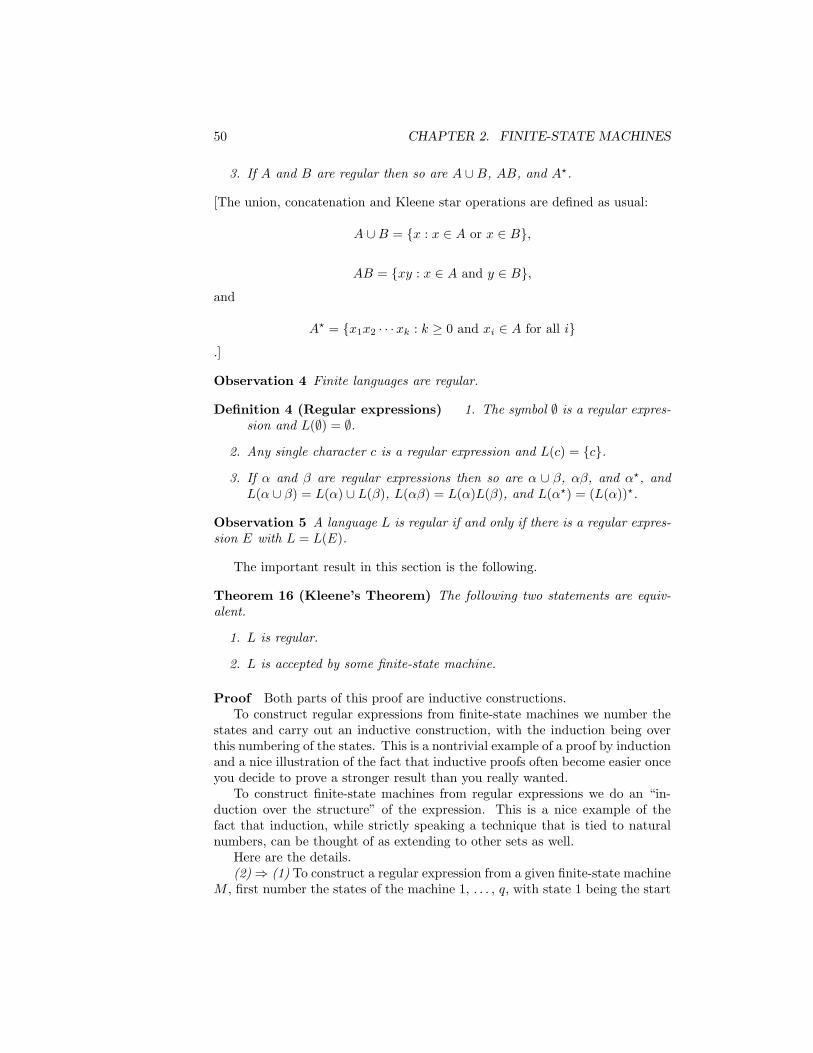
3. If A and B are regular then so are A ∪B, AB, and A?.
[The union, concatenation and Kleene star operations are defined as usual:
A ∪B = {x : x ∈ A or x ∈ B},
AB = {xy : x ∈ A and y ∈ B},and
A? = {x1x2 · · ·xk : k ≥ 0 and xi ∈ A for all i}.]
Observation 4 Finite languages are regular.
Definition 4 (Regular expressions) 1. The symbol ∅ is a regular expres-sion and L(∅) = ∅.
2. Any single character c is a regular expression and L(c) = {c}.3. If α and β are regular expressions then so are α ∪ β, αβ, and α?, and
L(α ∪ β) = L(α) ∪ L(β), L(αβ) = L(α)L(β), and L(α?) = (L(α))?.
Observation 5 A language L is regular if and only if there is a regular expres-sion E with L = L(E).
The important result in this section is the following.
Theorem 16 (Kleene’s Theorem) The following two statements are equiv-alent.
1. L is regular.
2. L is accepted by some finite-state machine.
Proof Both parts of this proof are inductive constructions.To construct regular expressions from finite-state machines we number the
states and carry out an inductive construction, with the induction being overthis numbering of the states. This is a nontrivial example of a proof by inductionand a nice illustration of the fact that inductive proofs often become easier onceyou decide to prove a stronger result than you really wanted.
To construct finite-state machines from regular expressions we do an “in-duction over the structure” of the expression. This is a nice example of thefact that induction, while strictly speaking a technique that is tied to naturalnumbers, can be thought of as extending to other sets as well.
Here are the details.(2) ⇒ (1) To construct a regular expression from a given finite-state machine
M , first number the states of the machine 1, . . . , q, with state 1 being the start

2.2. THE MYHILL-NERODE THEOREM 51
3
21
a
a
b
b
ab
Figure 2.18: Illustrating the notion of a string making a machine “pass through”states
state. Define Lkij to be the set of all strings which make the machine go from
state i into state j without ever “passing through” any state numbered higherthan k. For example, if the machine of Figure 2.18 happens to be in state 1 thenthe string ba will make it first go to state 2 and then to state 3. In this sequence1 → 2 → 3 we say that the machine “went through” state 2. It did not “gothrough” states 1 or 3, which are only the starting point and the endpoint inthe sequence. Since it did not go through any state numbered higher than 2 wehave ba ∈ L2
13. Other examples are babb ∈ L232 and a ∈ L0
23, in fact {a} = L023.
In this example, the language accepted by the machine is L313. In general, the
language accepted by a finite-state machine M is
L(M) =⋃
f
Lq1f (2.11)
where the union is taken over all accepting states of M . What’s left to show isthat these languages Lk
ij are always regular. This we show by induction on k.For k = 0, L0
ij is finite. It contains those characters that label a transitionfrom state i to state j. If i = j the empty string gets added to the set.
For k > 0,Lk
ij = (Lk−1ik (Lk−1
kk )?Lk−1kj ) ∪ Lk−1
ij . (2.12)
This equation amounts to saying that there can be two ways to get from statei to state j without going through states numbered higher than k. Either wego through k, or we don’t, corresponding to the subexpression before the unionand the subexpression after the union. Figure 2.19 illustrates this. Figure 2.20shows some of the steps in the construction of a regular expression from thefinite-state machine of Figure 2.18. We simplify the subexpressions as we go.Expression Ek
ij describes language Lkij : “L(Ek
ij) = Lkij .” Some parentheses are
omitted. λ is short for ∅?, hence L(λ) = {λ}, by the definition of the ?-operation.(We wouldn’t want to miss a chance to be obscure, would we?)

52 CHAPTER 2. FINITE-STATE MACHINES
i
L
k
j
L
L
ij
k-1
k-1
k-1
kk
kj
k-1
ikL
Figure 2.19: The pattern of induction for constructing the regular expressionsLk
ij in Kleene’s Theorem
(1) ⇒ (2) To construct finite-state machines from regular expressions weuse what is called “induction on the structure of the expression” or “structuralinduction.” This means that finite-state machines are first constructed for smallsubexpressions, then combined to form machines for larger subexpressions andultimately for the whole expression.
For example, if we want to convert the expression
E = (abb) ∪ (b(aa)?bab)
a machine M(aa)? for the subexpression (aa)? is shown in figure 2.21.For simplicity let’s adopt the convention that if a transition goes to a reject-
ing state from which the machine cannot escape anymore then we won’t drawthe transition, nor that “dead” state. This simplifies the picture for M(aa)? , seeFigure 2.22. A machine Mb is easier yet, see Figure 2.23. We can combine Mb
and M(aa)? to get Mb(aa)? , shown in Figure 2.24. Adding parts that correspondto subexpressions abb and bab completes the construction, see Figure 2.25. Thisseems easy enough, but what if the expression had been just slightly different,with an extra b in front:
E′ = (babb) ∪ (b(aa)?bab)
Then our construction would have gotten us this machine ME′ in Figure 2.26.This machine ME′ has a flaw: there are two transitions labeled b out of the
start state. When we run such a machine what will it do? What should it do,presented with such an ambiguity? Can we define the “semantics,” i.e., canwe define how such a machine is to run, in such a way that the machine ME′
accepts the very same strings that the expression E′ describes?

2.2. THE MYHILL-NERODE THEOREM 53
E011 = λ ∪ a E0
12 = b E013 = ∅
E021 = ∅ E0
22 = λ ∪ b E023 = a
E031 = b E0
32 = a E033 = λ
E132 = (E0
31(E011)
?E012) ∪ E0
32 = (b(λ ∪ a)?b) ∪ a = ba?b ∪ a
E111 = a? E1
12 = a?b E113 = ∅
E121 = ∅ E1
22 = λ ∪ b E123 = a
E131 = ba? E1
32 = ba?b ∪ a E133 = λ
E213 = (E1
12(E122)
?E123) ∪ E1
13 = (a?b(b?)?a) ∪ ∅ = a?bb?a
E211 = a? E2
12 = a?b+ E213 = a?bb?a
E221 = ∅ E2
22 = b? E223 = b?a
E231 = ba? E2
32 = ba?b+ E233 = (ba?b ∪ a)b?a
E311 = (E2
13(E233)
?E231) ∪ E2
11 = (a?bb?a((ba?b ∪ a)b?a)?ba?) ∪ a?
Figure 2.20: Converting the finite-state machine from Figure 2.18 into a regularexpression

54 CHAPTER 2. FINITE-STATE MACHINES
ba, b
b
a
a
Figure 2.21: The machine M(aa)?
a
a
Figure 2.22: The machine M(aa)? , a simplified drawing
b
Figure 2.23: The machine Mb
b
a
a
Figure 2.24: The machine Mb(aa)?
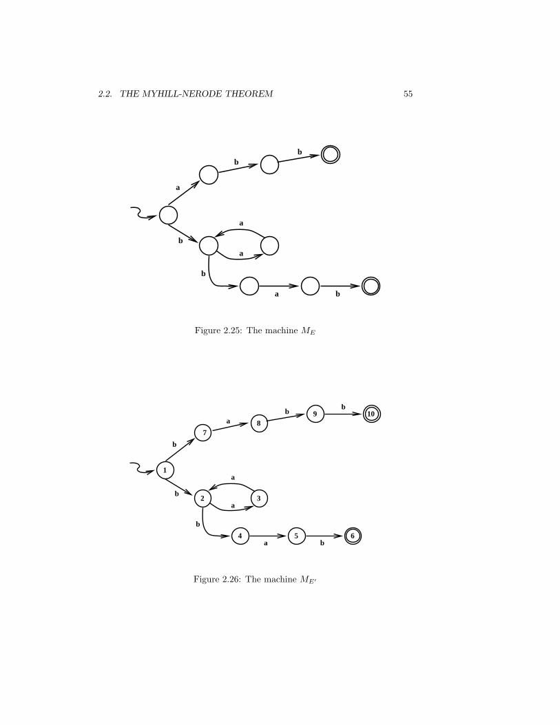
2.2. THE MYHILL-NERODE THEOREM 55
a
bb
a
a
b
b
ba
Figure 2.25: The machine ME
b
b
a
a
b
b
ba
98
7
1
3
65
2
4
10b
a
Figure 2.26: The machine ME′

56 CHAPTER 2. FINITE-STATE MACHINES
b
ba
a
a
b
b
ba
98
7
1
3
65
2
4
Figure 2.27: The machine ME′′
After reading an initial b, should ME′ be in state 2 or in state 7? We want toaccept both babb and baabab. Being in state 7 after the first b give us a chanceto accept babb; and being in state 2 gives us a chance to accept baabab. Thissuggests that the right way to run this machine is to have it be in both states 2and 7 after reading the first b.
With this way of running the machine, which states would it be in afterreading an a as the second character? In states 3 and 8. After reading a b asthe third character, it can only be in state 9. 7 After reading another b — fora total input string of babb — ME′ is in state 10 and accepts the input.
There is one more issue that this example does not address. What if somesuch machine ends up in a set of states some of which are accepting and someare rejecting? The expression
E′′ = (bba) ∪ (b(aa)?bab)
provides an example. Our construction will result in the machine ME′′ of Fig-ure 2.27. After reading bba, the machine is in state 5, which is rejecting, and instate 9, which is accepting. Since bba is a string described by E′′, it should beaccepted by ME′′ . That settles the issue: a string is accepted if at least one ofthe states it puts the machine in is an accepting state.
Our conventions about running these machines and knowing when a stringis accepted are the “semantics of nondeterministic finite-state machines.” These
7This could be up to some discussion depending on how we view our convention of notdrawing a “dead” state, i.e., a rejecting state from which the machine cannot escape. If wetake the view that the state is there — we just don’t draw it — then at this point we shouldsay that the machine would be in state 9 and that invisible state, say 11. This is clumsy. It ismore elegant — although ultimately of no important consequence — to say that the machineis only in state 9.

2.2. THE MYHILL-NERODE THEOREM 57
b
9
1
65
2,7b
b
a
2 3
a
a
3,8
4
b
a
b
b
a
10
Figure 2.28: Converting ME′ into a deterministic machine
conventions can be applied to more powerful programs as well (and we will doso in a later chapter on computational complexity, where the concept of nonde-terminism will play a crucial role in defining a class of computational problems).“Nondeterministic C,” for example, could be C with the extra feature of a non-deterministic branch:
( nondet-branch; x = 0; x = 1; )
The way to think about the execution of such nondeterministic programs is thatthere is more than one path of execution. Tracing the execution results in atree and a program is said to accept its input if at least one of the paths leadsto acceptance.
Can we convert this new kind of machine into a standard (deterministic)finite-state machine? This task amounts to a search of the “execution tree,”which we do in a breadth-first approach. Figure 2.28 gives an example, convert-ing the machine ME′ into a deterministic one. The states of the deterministicmachine are the sets of states of ME′ . (Many of these sets of states may notbe reachable from the start state and can be discarded.) In the deterministicmachine, the state reached from a state A via a transition c, δ(A, c), is the setof those states b of ME′ to which there is a c-transition (in ME′) from somestate a ∈ A.
The algorithm for constructing a nondeterministic machine from a regularexpression is easier to describe if we allow yet another form of nondetermin-istic behavior: making a “spontaneous” transition, i.e., a transition that doesnot consume an input character. The standard term is a “λ-transition.” Theinductive algorithm for constructing a (nondeterministic) finite-state machineME from an arbitrary regular expression E then works as shown in Figure 2.29.An example that uses all the parts of this algorithm is the machine shown inFigure 2.30.

58 CHAPTER 2. FINITE-STATE MACHINES
1. M∅ is the following machine:
2. For any single character c, Mc is the following machine:
c
3. If α and β are regular expressions then Mα∪β, Mαβ, andMα? are constructed from Mα and Mβ as shown below.
λ
α
βM
M
λ
Constructing Mα∪β from Mα and Mβ
M α
λ
M β
λ
Constructing Mαβ from Mα and Mβ
αM
λ
λ
λ
Constructing Mα? from Mα
Figure 2.29: An algorithm for converting regular expressions to finite-state ma-chines

2.2. THE MYHILL-NERODE THEOREM 59
a a
λ
λ
λλ
λ
λλa b bλ
λ
Figure 2.30: The machine M(aa)?∪(a(bb)?)
a
a
bb
b
a
a
Figure 2.31: A deterministic version of M(aa)?∪(a(bb)?)
Nondeterministic machine with λ-transitions can be turned into determin-istic ones with the same set-of-states approach used earlier. For example, themachine in Figure 2.30 turns into the machine in Figure 2.31.
This concludes the proof of Kleene’s Theorem.
Given that finite-state machines and regular expressions are equivalent concepts, Finite-State Machines orRegular Expressions?we can choose to approach some problem in terms of one or the other. Some
questions are easier to deal with in terms of finite-state machines, others interms of regular expressions. Here are some examples, all of them variations ofthe question of which languages are regular:
Question 1. Is the set of binary numbers that are divisible by 2 regular?

60 CHAPTER 2. FINITE-STATE MACHINES
0
0
1
Figure 2.32: A piece of a finite-state machine
This is easy in either domain. The right regular expression is (0 ∪ 1)?0.
Question 2. Is the set of binary numbers that are divisible by 3 regular?
The answer is yes, but it seems nearly impossible to build a suitable regularexpression. After all, what is the common pattern of 11, 110, 10000000010,1001? Yet it is not all that hard to build a finite-state machine for this language,with the right approach anyway. The Myhill-Nerode Theorem tells us that wewould have to figure out exactly what it is that we want to keep track of as theinput gets processed.
If we know that the input so far was a number that was divisible by 3,then we know that after reading one more 0, the number is again divisible by3. (This is so because reading that 0 amounted to multiplying the previousnumber by 2.) What if a 1 had been read instead? This would have amountedto multiplying the previous number by 2 and adding 1. The resulting number,when divided by 3, would yield a remainder of 1. This translates into a pieceof a finite-state machine shown in Figure 2.32. The complete machine is shownin Figure 2.33. The four equivalence classes of ≡L (and hence the states of theminimal machine for L) are {λ} and the three sets of binary numbers which,when divided by three, yield a remainder of 0, 1, and 2. These remainders areused as the labels of the three states.
Question 3. Are regular languages closed under union? I.e., if A and B areregular, is their union A ∪B regular as well?
The answer is yes. It follows from the definition of regular sets and expres-sions. In terms of finite-state machines, this requires an argument involvingnondeterministic machine (as used in the proof of Kleene’s Theorem).
Question 4. Are regular languages closed under complement? I.e., if A isregular, is A = {x : x /∈ A} regular as well?
This is most easily dealt with in terms of finite-state machines. If M is afinite-state machine for A then a finite-state machine for A can be obtained byturning accepting states into rejecting ones, and vice versa. There is no equallysimple argument in terms of regular expressions.

2.2. THE MYHILL-NERODE THEOREM 61
λ
1
0
0
0
1
1 112
0
0
Figure 2.33: A finite-state machine for binary numbers divisible by 3
Question 5. Are regular languages closed under set difference? I.e., if A andB are regular, is their difference A− B = {x : x ∈ A and x /∈ B} regularas well?
There is a construction based on finite-state machine that proves this closureresult and is interesting in its own right.
Question 6. Is the set of syntactically correct C programs regular?
It is not, and the only proof method presented so far is to argue that thereare infinitely many equivalence classes induced by ≡L. Here is an infinite list ofnonequivalent strings:
main () { int x; x = (main () { int x; x = ((main () { int x; x = (((main () { int x; x = ((((main () { int x; x = (((((...
This shows that parsing programs, which is a necessary part of compilingthem, cannot be done with an amount of memory that does not depend on theinput that is being parsed. As we will see in the next chapter, it takes a “stack”to parse.

62 CHAPTER 2. FINITE-STATE MACHINES
2.3 The Pumping Lemma for Regular Languages
“Pumping” is a second technique to prove nonregularity. It is interesting in itsown right, although no more powerful than the analysis of ≡L that we havediscussed already in Sections ??. Pumping is important if for no other reasonthen because unlike the analysis of ≡L in Myhill-Nerode, pumping argumentsalso work for the more powerful programs we will consider in the next chapter.
Lemma 3 Pumping Lemma for Regular Languages. If L is a regularlanguage then there is a constant k such that for every string w in L of lengthk or more the following is true.
There are three strings, u, v, x, such that
1. w = uvx, and
2. for all i ≥ 0, uvix ∈ L, and
3. |v| > 0.
Let’s use this Lemma to prove that the language L = {anbn : n ≥ 1} is notregular.
Assuming it was. Then the Lemma applies. Let k be the constant said toexist in the Lemma. Consider the string w = akbk. The length of w is k ormore (in fact, 2k), hence statements (1) — (3) from the Lemma apply, implyingthat it is possible to split w into three parts, w = uvx, such that |v| > 0 anduv2x ∈ L. But this is not true. No matter what three-way split of w one tries,uv2x is never of the form of equal numbers of a’s and b’s.
(One can come up with a more detailed argument for this. The challenge isto cover all ways in which the strings could get divided up into three pieces. Anadded challenge is to come up with a concise argument. Here is an attempt:
The substring v cannot contain more than one type of character becauseotherwise v2 contains characters in an order not permitted in L. Hence at mostone type of character take part in the “pumping” from uvx to uv2x, whichtherefore does not contain equal numbers of both characters anymore.)
This contradiction shows that L is not regular.
The Pumping Lemma can be stated as follows.Why is this so messy?
L regular
=⇒There is a constant k such that
for all strings w ∈ L with |w| ≥ kthere are strings u, v, x with w = uvx and |v| > 0 such that
for all i ≥ 0, uvix ∈ L.

2.3. THE PUMPING LEMMA FOR REGULAR LANGUAGES 63
The above statement is of the form “L regular ⇒ B,” where B is thatcomplicated statement with four alternating quantifiers. Since we are trying toprove that some languages are not regular, a more useful version of the statementis “L not regular ⇐ ¬B.” Spelled out in detail, this version reads
L not regular
⇐=
For all constants kthere is a string w ∈ L with |w| ≥ k such that
for all strings u, v, x with w = uvx and |v| > 0there is an i ≥ 0 with uvix 6∈ L.
Thus, we can prove that some language L is not regular by proving the abovefour-line statement ¬B : “For all . . . 6∈ L”. This is what we did in the previousexample. Here is another one.
Let’s take the language that consists of strings like Another Example
1234+111=134510000+10000=20000
1020304+505=102080911111+22222=33333
The language consists of strings of the form α + β = γ that represent a correctequation between decimal integers.
This language L is not regular, a fact we prove by proving the statement“¬B” above.
How do we prove something “for all constants k”? By starting out theproof by saying “Let k be an arbitrary constant” and carrying the k along as aparameter of the argument.
What’s next? We need to show that there exists a string w with certainproperties. To show this, all we need to do is exhibit one such string. In thisexample, let’s pick w to be the string
1 · · · 1︸ ︷︷ ︸k
+ 2 · · · 2︸ ︷︷ ︸k
= 3 · · · 3︸ ︷︷ ︸k
(Note how the k plays its role.) What’s the next step? We have to show thatfor all strings u, v, x which represent a three-way breakup of w (“w = uvx” )and which don’t have the second piece empty ( “|v| > 0” ), there is a constanti with uvix 6∈ L. This is the hard part of the proof because we somehow haveto provide an argument that covers all possible such three-way breakups of w.It can be done, by dealing with an exhaustive set of cases. Here is such anexhaustive set of cases for this example.
Case 1. v contains the =. Then uv0x 6∈ L if for no other reason then becauseit does not have an = in it.

64 CHAPTER 2. FINITE-STATE MACHINES
Case 2. v does not contain the =. Then v lies entirely on one side of the = andpumping (with any i 6= 1) changes that side of the equation but not theother, thus creating a string outside of L.
Exercises
Ex. 2.1. Draw the smallest finite-state machine M for the language of allbitstrings that contain the substring 011.
Ex. 2.2. Draw the smallest finite-state machine M for the language of allbitstrings that contain the substring 011. (Make sure you provide a 0 and a 1transition out of every state.)
Ex. 2.3. Carry out the minimization algorithm of Figure 2.6 for the finite-Minimizing finite-statemachines state machine shown below. (Show the development of the “clusters” of states
just like Figure 2.8 did.)
Ex. 2.4. Draw a finite-state machine on which the minimization algorithmruns through more than 10 passes.
Ex. 2.5. Let L be the language of all bitstrings that contain a run of threeThe Myhill-NerodeTheorem consecutive 0s. Is it true that 01 ≡L 001? Explain.
Ex. 2.6.
1. If L is the language of all bitstrings that start with a 1 and end with a 0,then 01 ≡L 00.
2. If L is the language of all bitstrings of length 8, then 0001 ≡L 0011.
3. Let L be the language of all bitstrings x such that x contains at least one0. (For example, 01 ∈ L, 1111 6∈ L.) How many equivalence classes does≡L induce?
4. Let L be the language of all bitstrings x such that x contains at least one0 and at least one 1. (For example, 01 ∈ L, 1111 6∈ L, 00 6∈ L.) How manyequivalence classes does ≡L induce?
Ex. 2.7. Let L be the language of binary strings whose third bit from theend is a 1. Give one string from each of the equivalence classes induced by ≡L.
Ex. 2.8. Same for the language of bitstrings whose first two bits are equal toits last two bits.

2.3. THE PUMPING LEMMA FOR REGULAR LANGUAGES 65
Ex. 2.9. Give one representative of each equivalence class of ≡L for L = {x : xcontains the substring 000}.
Ex. 2.10. Consider the following language L over the alphabet Σ = {a, b, $}:
L = {x$y : x, y ∈ {a, b}+ and x does not start with the same letter as y}
For every equivalence class of ≡L, give one shortest string from the class.
Ex. 2.11. Is it true that x ≡L y implies xz ≡L yz? Is it true that xz ≡L yzimplies x ≡L y? When your answer is no, give a counterexample.
Ex. 2.12. Are the two relations ≡L and ≡L (that’s L, the complement ofL) always the same, for any given L? Either argue that they are, or show anexample were they aren’t?
Ex. 2.13. (b) Do the partitions that go with ≡L and with ≡Lrev (that’sLrev = {xrev : x ∈ L}) always have the same equivalence classes? Either arguethat they always do, or show an example were they don’t? (xrev is x writtenbackwards.)
Ex. 2.14. Which of the following languages is regular? (Just circle “Yes” or“No” for each language. Do not give explanations.)
1. The language described by (ab(a?)?(b? ∪ (aab)?))
2. Strings containing the word while
3. Strings containing two opening parentheses with no closing parenthesis inbetween the two, e.g. “(a)b)c(d(e(f”
4. Strings containing more opening parentheses than closing ones,e.g. “())(((”
5. Strings containing all their opening parentheses before all their closingones, e.g. “((x(y-/)”
6. Strings of even length whose first half and second half both start with thesame letter, e.g. “abcabaeeee”
Ex. 2.15. Consider two finite-state machines that accept languages A and Band consider their cross-product machine. As discussed in class, one can alwayschoose the accepting states of the cross-product machine such that it acceptsA ∩B.
Can one always choose the accepting states of the cross-product machinesuch that it accepts . . .

66 CHAPTER 2. FINITE-STATE MACHINES
1. A ∪B ?
2. A−B ? (That’s {x : x ∈ A and x /∈ B}.)3. AB ? (That’s A concatenated with B: {xy : x ∈ A and y ∈ B}.)4. Strings in A ∪B of length five or more?
5. A ?
Ex. 2.16. Derive an asymptotic bound on the length of the expression con-Regular Expressionsstructed from a finite-state machine in the proof of Kleene’s Theorem. Assumewe are dealing with bitstrings only.
Ex. 2.17. Consider the problem of taking an arbitrary nondeterministicNondeterministicMachines finite-state machine that accepts some language A and modifying the machine
to accept the complement of A instead (i.e., all the strings that are not in A).Does the following approach work: Make all rejecting states of the nonde-
terministic machine into accepting states and all accepting states into rejectingstates?
Briefly explain your answer.
Ex. 2.18. For any k ≥ 0 let Lk be the language of bitstrings whose first kbits equal their last k bits. How many states does a deterministic finite-statemachine for Lk need? Same for a nondeterministic machine. How long is aregular expression for Lk?
Ex. 2.19. Give three properties that are decidable for finite-state machinesbut undecidable for arbitrary programs.
Ex. 2.20. Which of the languages in Figure ?? are regular?
Ex. 2.21. Consider creating the cross-product machine of two given ma-Cross-ProductConstruction chines and choosing the accepting states such that the new machine accepts the
intersection of the languages of the two old machines.(a) Give an example where the cross-product machine is minimal.(b) If the cross-product machine is minimal, does that imply that the two
“factors” in the product had to be minimal? Give an argument or a counterex-ample.
Ex. 2.22. For any program p define Lp to be the set of input strings on whichMiscellaneousthe program prints the word “Yes” and terminates. Is it decidable whether ornot a program p has a regular language Lp? Briefly justify your answer.
Ex. 2.23. Let Fsm-Equivalence be the problem of deciding, given two finite-state machines P and Q, whether or not L(P ) = L(Q). Let Fsm-Emptiness

2.3. THE PUMPING LEMMA FOR REGULAR LANGUAGES 67
be the problem of deciding, given a finite-state machine M , whether or notL(M) = ∅. Describe how a cross-product construction can be used to transformFsm-Equivalence into Fsm-Emptiness.
Ex. 2.24. Construct a finite-state machine for the language {x : x ∈ {0, 1}?
and x /∈ {000, 001}?}. First construct a nondeterministic machine that is assmall as possible, then apply the subset construction, then minimization.
Ex. 2.25. For two of the nonregular languages in Figure ?? use the pumpinglemma to prove that they are not regular.
Ex. 2.26. Prove that every infinite regular language contains a string whoselength is not a prime number.
Ex. 2.27. Prove that the set of strings that are finite prefixes of this infinitestring-0-1-10-11-100-101-110-111-1000-1001-1010-1011- · · ·is not regular.
Ex. 2.28. Formulate a stronger version of the pumping lemma, one that saysnot only that pumping occurs somewhere in a long enough string but that itoccurs within every long enough substring. Use this stronger version to provetwo languages from 8 Figure ?? not regular which cannot be proven not regularwith the original weaker version.
8To do: This is not in the sample solutions yet.

68 CHAPTER 2. FINITE-STATE MACHINES

Chapter 3
Context-Free Languages
3.1 Context-Free Grammars
As we saw at the end of the previous chapter, one feature of programminglanguages that makes them nonregular is the arbitrary nesting of parenthesisin expressions. Regular expressions cannot be used to define what syntacticallycorrect expressions look like. “Context-free grammars” can.
An example of a context-free grammar is this:
E → E + E
E → E × E
E → ( E )E → x
E → y
The way this grammar — call it G1 — is used is to start with the symbol onleft of the arrow in the first line, E. This is the “start symbol” — the string oflength 1 we start out with. We then grow that string by repeatedly replacingwhat’s on the left-hand side of an arrow with what’s on the right-hand side.The best way to keep track is a tree:
69

70 CHAPTER 3. CONTEXT-FREE LANGUAGES
E
E
y X ( x + y )
E
x +
E
E EEE
There are choices of which replacements to make. The choices made aboveresulted in a tree whose leaves, read from left to right, read x+y× (x+y). Thegrammar G1 is said to “derive” that string: x + y × (x + y) ∈ L(G1). The treeis a “derivation tree” for the string.
Derivation trees are also called “parse trees.” They are used in compilersto know how to translate a given expression, or a whole program, into machinelanguage, and in interpreters to know how to evaluate an expression, or interpreta whole program.
Our sample grammar does not serve that purpose well, though. This isbecause it allows a second derivation tree for the same string:
E
X ( x + y )
E E
E
+
E
x
E
E
E
y
Such a grammar is said to be “ambiguous.” The two parse trees for the stringx + y× (x + y) lead to two different evaluations of the expression. If we plug inx = 1 and y = 5, the first tree leads to a value of 36 for the expression, whereasthe second one leads to a value of 31. Of the two trees, only the first one matchesour conventions about the precedence of arithmetic operations. The first one is“right,” the second one is “wrong.” The problem is, this grammar G1, while itdoes perfectly well describe the language in question, does not help us define theone and only “correct” way to parse each string in the language. The following

3.2. PARSING 71
grammar G2 does do that:
E → E + T
E → T
T → T × F
T → F
F → ( E )F → x
F → y
This grammar only allows one derivation tree, the “right” one, for any arithmeticexpressions involving +, ×, parentheses, and the variables x and y. The treefor the expression x + y × (x + y) is:
T
E
F
E
x + y X ( x + y )
F F
E
T TT
FF
T
E
3.2 Parsing
Recursive-Descent Parsing
A grammar like G2 above is easily turned into a parser, i.e., a program thatdetermines whether or not a given input string is in the language and does so(necessarily) by building a parse tree, implicitly or explicitly. See Figure 3.1.The program is nondeterministic, though — certainly a flaw we do not want totolerate for very long.
In what sense does this program “parse” expressions?

72 CHAPTER 3. CONTEXT-FREE LANGUAGES
main ( )
{
E();
if (getchar() == EOF)
ACCEPT;
else
REJECT;
}
E ( )
{
nondet-branch:
{E(); terminal(’+’); T();}
{T();}
}
T ( )
{
nondet-branch:
{T(); terminal(’*’); F();}
{F();}
}
F ( )
{
nondet-branch:
{terminal(’(’); E(); terminal(’)’);}
{terminal(’x’);}
{terminal(’y’);}
}
terminal( char c )
{
if (getchar() != c)
REJECT;
}
Figure 3.1: A nondeterministic recursive-descent parser

3.2. PARSING 73
Being a nondeterministic program, the program as a whole is said to acceptan input string if there is at least one path of execution that accepts it. Consideragain the string x+y× (x+y). The one path of execution that results in accep-tance is the one where the first execution of E in turn calls E, terminal(’+’),and T. These calls correspond to the children of the root of the derivation tree.If we chart the calling pattern of the accepting execution we end up drawingthe parse tree. The accepting computation looks like a preorder traversal of theparse tree of the input string.
The above construction shows how to turn any context-free grammar intoa program that is like the finite programs of Chapter 2 except that it usestwo additional features: recursion and nondeterminism. Such programs areoften called “pushdown machines” or “pushdown automata (pda’s).” They areequivalent to finite-state machines augmented by a stack to implement recursion.Thus the above example generalizes to the following theorem.
Theorem 17 For every context-free grammar G there is a pushdown machineM with L(M) = L(G).
The converse is also true, providing a complete characterization of context-freelanguages in terms of a type of program.
Theorem 18 For every pushdown machine M there is a context-free grammarG with L(M) = L(G).
(We don’t prove this here.)
Deterministic Parsing
Intrinsically Nondeterministic Context-Free Languages
With regular languages and finite-state machines it was always possible to re-move the nondeterminism from the machines. The trick was to replace statesby sets of states. This worked because the power set (set of subsets) of a finiteset was again a finite set. This approach does not work for pushdown machinesbecause a set of stacks, or even just two stacks, cannot be implemented with asingle stack. Without giving any proof of this, here is an example of a grammarthat derives an intrinsically nondeterministic language. The language is verysimple, all bitstrings of odd length whose middle character is a 1.
S → B S B | 1B → 0 | 1
To parse this language with a pushdown machine, nondeterminism is needed.We do not prove this here, but the intuition is that the parser must keep buildingup a stack of recursive calls for the first half of the input string and climb out ofthe recursion during the second half. The problem is, with information limitedby a constant amount, it is not possible to know when the second half starts.

74 CHAPTER 3. CONTEXT-FREE LANGUAGES
A “Predictive” Recursive-Descent Parser
(The example is after Aho and Ullman, Principles of Compiler Design, 1978,p.176ff.)While a deterministic recursive-descent parser does not exist for all context-free languages, some languages are simple enough to yield to such an approach.For example, the grammar for arithmetic expressions used earlier can be trans-formed, without changing the language, into the following:
E → TE′
E′ → +TE′ | λ
T → FT ′
T ′ → ×FT ′ | λ
F → ( E )F → x
F → y
The work done by the first two productions version, which was to generateintermediate strings of the form
T + T + · · ·+ T
is done by the first two productions of the new version. The new grammarleads to a parser in which the decision which of the nondeterministic paths hasa chance of leading to acceptance of the input can be made on the basis oflooking at the next character of the input. This is so because whenever thegrammar has several right-hand sides for the same left-hand symbol, the right-hand sides differ in their first character. The resulting deterministic parser inshown in Figure 3.2.
A General Parsing Algorithm
Instead of using nondeterminism, which is impractical even when implementedby a deterministic tree-traversal, one can use a “dynamic programming” ap-proach to parse any context-free language. Dynamic programming is a typeof algorithm somewhat resembling “divide-and-conquer,” which inductively (orrecursively, depending on the implementation) builds up information about sub-problems. It typically has O(n3) time complexity.
There are two steps to using this technique. First, we change the grammarinto “Chomsky Normal Form,” then we apply the actual dynamic programmingalgorithm.
Every context-free grammar can be converted into an equivalent one in whichChomsky Normal Formeach production is of one of the two forms

3.2. PARSING 75
main ( )
{
E();
if (getchar() == EOF)
ACCEPT;
else
REJECT;
}
E ( ) { T(); E’(); }
E’ ( )
{
if (NEXTCHAR == ’+’)
{terminal(’+’); T(); E’();}
else
// do nothing, just return
}
T ( ) { F(); T’(); }
T’ ( )
{
if (NEXTCHAR == ’*’)
{terminal(’*’); F(); T’();}
else
// do nothing, just return
}
F ( )
{
switch (NEXTCHAR)
{
case ’(’: {terminal(’(’); E(); terminal(’)’);}
break;
case ’x’: terminal(’x’);
break;
case ’y’: terminal(’y’);
break;
default: REJECT;
}
}
...
Figure 3.2: A deterministic recursive-descent parser

76 CHAPTER 3. CONTEXT-FREE LANGUAGES
A → BC
A → a
where A, B, C are syntactic variables, not necessarily different ones, and a isa terminal symbol. This form of a context-free grammar is called “ChomskyNormal Form.” To see how this conversion can be done consider this production:
A → BCdEfG (3.1)
The production 3.1 can equivalently be replaced by the set of productions
A → BCDEFG (3.2)D → d
F → f
and the production 3.2 can then be replaced by the set of productions
A → BC ′
C ′ → CD′
D′ → DE′
E′ → EF ′
F ′ → FG
(The example below is from Hopcroft and Ullman, Introduction to AutomataTheory, Languages, and Computation, 1979, pp. 140-1.)
Figure 3.3 shows an example. The “length = 2, starting position = 3” fieldCYK Parsing: AnExample of “Dynamic
Programming”contains all those variables of the grammar from which one can derive the sub-string of length 2 that starts at position 3. (The string is ab. The variables areS and C.) The rows of the table get filled in from top (length=1) to bottom(length=5). The whole string is in the language if the start symbol of the gram-mar shows up in the bottom field. Filling in a field makes use of the contentsof fields filled in earlier, in a pattern indicated by the two arrows in the Figure.
The algorithm is easily modified to yield a parse tree, or even sets of parsetrees.
3.3 The Pumping Lemma for Context-Free Gram-mars
The grammar
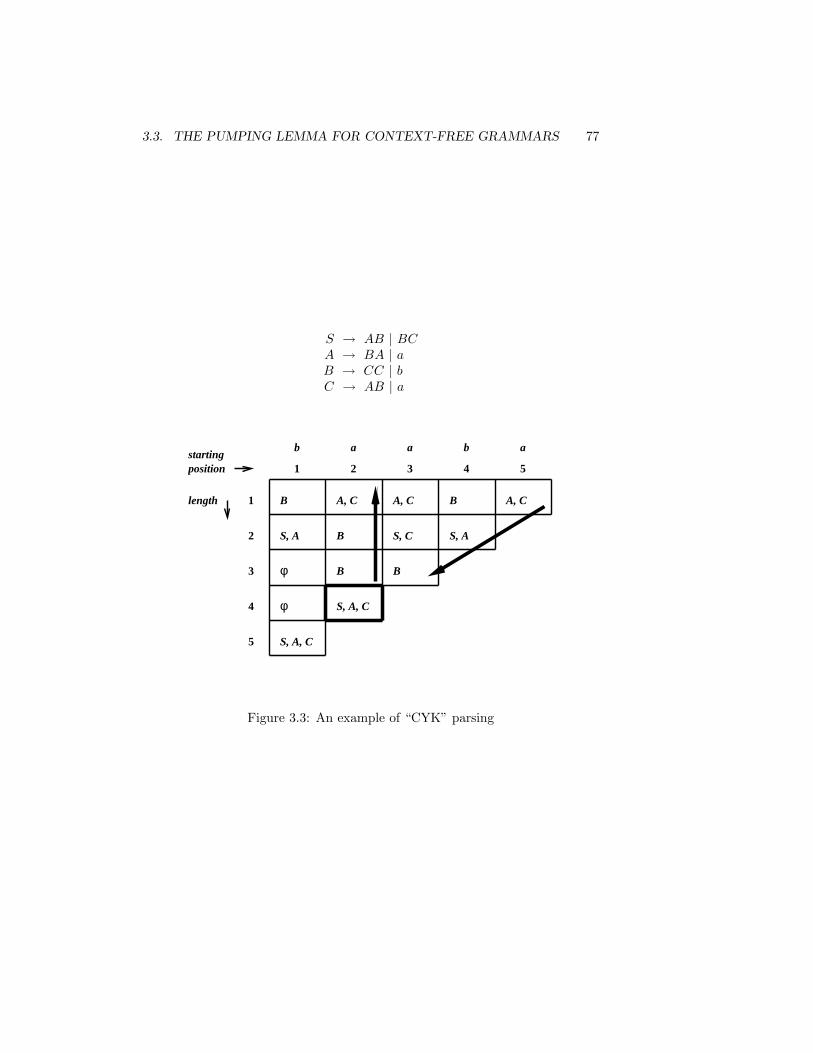
3.3. THE PUMPING LEMMA FOR CONTEXT-FREE GRAMMARS 77
S → AB | BCA → BA | aB → CC | bC → AB | a
54321
abaab
5
4
3
2
1
startingposition
length
S, A, C
φ
φ
S, A
B A, C
B
B
S, A, C
B
S, C
A, C B
S, A
A, C
Figure 3.3: An example of “CYK” parsing

78 CHAPTER 3. CONTEXT-FREE LANGUAGES
S → 0 S 1 | 0 1
generates the language
L4 = {0n1n|n ≥ 1}.(0n means a string of n 0s.)
Similar grammars generate
L5 = {0n1n0m1m|n,m ≥ 1},
L6 = {anbmcn|n,m ≥ 1},
L7 = {anbmcmdn|n,m ≥ 1}.If we think of 0, a, and b as opening parentheses and 1, c, and d as closingparentheses, then these language all are examples of balanced parentheses.1
More complicated languages arise if we try to have equal numbers of not justtwo but three or more different characters, as for example in
L8 = {anbncn : n ≥ 1},and if we match numbers of characters beyond a nesting pattern, as for examplein
L9 = {anbmcndm : n,m ≥ 1}.If you try to write context-free grammars for L8 and L9, you sooner or later
get frustrated trying to achieve the specified equalities between the exponents(i.e., the numbers of repetitions of characters) in the definitions of these lan-guages. In fact,
Theorem 19 L8 and L9 are not context-free.
The languages L8 and L9 are of no practical interest. But after we develop aproof technique for showing that these languages are not context-free we will beable to use that technique to show that some aspects of programming languagesare not context-free either.
The proof of Theorem 19 uses a “cutting-and-pasting” argument on the parsetrees of context-free grammars. It is the most common argument for provinglanguages not to be context-free. The heart of the argument is that everycontext-free language has a certain “closure” property: The fact that certainstrings are in the language forces other strings to be in the language as well. A
1L7 is an example of nesting of different types of parentheses. Replace a and d by openingand closing parentheses and b and c by opening and closing square brackets. Then L7 becomes{(n[m]m)n|n, m ≥ 1}.

3.3. THE PUMPING LEMMA FOR CONTEXT-FREE GRAMMARS 79
>= n leaves
>= log n
height
u v y z
A
A
x
repetitionb
Figure 3.4: Illustrating the proof of Theorem 19
language that does not have the closure property cannot be context-free. Thedetails of that closure property are developed next.
If a language L is context-free there is, by definition, a context-free grammarG that generates L, L = L(G). Let b be the maximum length of right-handsides of productions of G. In other words, b is a bound on the maximum numberof children for nodes in parse trees of G. Then a parse tree with n leaves mustbe of height at least logb n, where height is defined to be 0 for a tree consistingof a single node. This means that a tree with n leaves must have a path fromthe root to a leaf with at least logb n − 1 interior nodes. What if n is so largethat logb n− 1 exceeds the number of different left-hand sides of productions inG? (These are also called “syntactic variables.”) Then some syntactic variablemust show up at least twice along that path. Figure 3.4 illustrates this.
Pick such a variable, call it A, and pick two occurrences of A along onepath. These two occurrences of A split the string w that the tree derives intofive parts, labeled u, v, x, y, z in Figure 3.4. (The substring vxy is derivedfrom the first of the two occurrences of the variable A, the substring x from thesecond occurrence.)
Knowing that we can derive x from A, the tree shown in the top half ofFigure 3.5 is also a parse tree in this grammar. It derives the string uxz. Thereare other trees we can construct. For example, as illustrated in the bottom halfof Figure 3.5, the second occurrence of A can be made to derive vxy, resultingin a tree that derives the string uvvxyyz. No need to stop there. We can buildtrees that derive uvvvxyyyz, uvvvvxyyyyz, in fact any string uvixyiz for anyi ≥ 2.
For i = 0, 1, the string uvixyiz becomes uxz and uvxyz, respectively. Thislets us summarize the effect of all this cutting-and-pasting of trees as the fol-

80 CHAPTER 3. CONTEXT-FREE LANGUAGES
A
xzu
xv
u z
A
A
A
y
v y
Figure 3.5: Deriving uxz and uvvxyyz

3.3. THE PUMPING LEMMA FOR CONTEXT-FREE GRAMMARS 81
lowing
Lemma 4 (Pumping Lemma for Context-Free Languages, Version 1)If L is an context-free language then there is a constant k such that for everystring w in L of length k or more the following is true.
There are five strings, u, v, x, y, z, such that
1. w = uvxyz, and
2. for all i ≥ 0, uvixyiz ∈ L, and
3. |vy| > 0.2
This lemma is strong enough to let us prove that the language L8 = {anbncn :n ≥ 1} from Theorem 19 is not context-free. (We will need to add one morerefinement before we can handle L9.)
Proof that L8 is not context-free. Assuming it was. Then Lemma 4 ap-plies. Let k be the constant said to exist in Lemma 4. Consider the stringw = akbkck. The length of w is k or more (in fact, 3k), hence statements (1) —(3) from the Lemma apply, implying that it is possible to split w into five parts,w = uvxyz, such that |vy| > 0 and uv2xy2z ∈ L8. But this is not true. Nomatter what five-way split of w one tries, uv2xy2z is never of the form of equalnumbers of a’s, b’s, and c’s following each other.3 This contradiction shows thatL8 is not context-free.
The Pumping Lemma can be stated as follows. Why is this so messy?
L context-free
=⇒There is a constant k such that
for all strings w ∈ L with |w| ≥ kthere are strings u, v, x, y, z with w = uvxyz and |vy| > 0 such that
for all i ≥ 0, uvixyiz ∈ L.2This last part of the statement we did not prove. The proof is left as an exercise. The
statement is saying that not both of v and y are empty.3One can come up with a more detailed argument for this. The challenge is to cover all
ways in which the strings could get divided up into five pieces. An added challenge is to comeup with a concise argument. Here is an attempt:
The substring v cannot contain more than one type of character because otherwise v2
contains characters in an order not permitted in L8. The same is true for y. Hence at mosttwo types of characters take part in the “pumping” from uvxyz to uv2xy2z, which thereforedoes not contain equal numbers of all three characters anymore.
82 CHAPTER 3. CONTEXT-FREE LANGUAGES
What makes such a statement hard to digest are the alternations of “for all”with “there is/are,” akin to the nesting of loops in a program.4
The above statement is of the form “L context-free ⇒ B,” where B is thatcomplicated statement with four alternating quantifiers. Since we are tryingto prove that some languages are not context-free, a more useful version of thestatement is “L not context-free⇐ ¬B.” Spelled out in detail, this version reads
L not context-free
⇐=
For all constants kthere is a string w ∈ L with |w| ≥ k such that
for all strings u, v, x, y, z with w = uvxyz and |vy| > 0there is an i ≥ 0 with uvixyiz 6∈ L.
Thus, we can prove that some language L is not context-free by proving theabove four-line statement ¬B : “For all . . . 6∈ L”. This is what we did in theprevious example. Here is another one.
Let’s take the language that consists of strings likeAnother Example
1234+111=134510000+10000=20000
1020304+505=102080911111+22222=33333
The language consists of strings of the form α + β = γ that represent a correctequation between decimal integers.
This language L is not context-free, a fact we prove by proving the statement“¬B” above.
How do we prove something “for all constants k”? By starting out theproof by saying “Let k be an arbitrary constant” and carrying the k along as aparameter of the argument.
What’s next? We need to show that there exists a string w with certainproperties. To show this, all we need to do is exhibit one such string. In thisexample, let’s pick w to be the string
1 · · · 1︸ ︷︷ ︸k
+2 · · · 2︸ ︷︷ ︸k
= 3 · · · 3︸ ︷︷ ︸k
4This this called an “alternation of quantifiers.” There are formal results that say thatadding a level of alternation makes statements harder in the sense that even if we had aprogram that could determine the truth of statements with q alternations of quantifiers, thiswould not enable us to build a program that determines truth of statements with q + 1quantifiers. (The concept of transformations is rearing its ugly head.) Look for the subjectof “the arithmetic hierarchy” in textbooks on recursive function theory if you want to readabout this.

3.3. THE PUMPING LEMMA FOR CONTEXT-FREE GRAMMARS 83
(Note how the k plays its role.) What’s the next step? We have to show that forall strings u, v, x, y, z which represent a five-way breakup of w (“w = uvxyz”) and which don’t have the second and fourth piece both empty ( “|vy| > 0”), there is a constant i with uvixyiz 6∈ L. This is the hard part of the proofbecause we somehow have to provide an argument that covers all possible suchfive-way breakups of w. It is tedious, but it can be done, by dealing with anexhaustive set of cases. Here is such an exhaustive set of cases for this example.
Case 1. Either v or y or both contain the + and/or the =. Then uv0xy0z 6∈ Lif for no other reason then because it does not have a + and an = in it.
Case 2. Neither v nor y contain the + or the =.
Case 2.1. Both v and y lie on the same side of the =. Then pumping(with any i 6= 1) changes that side of the equation but not the other,thus creating a string outside of L.
Case 2.2. v lies entirely on the left side of the equation and y lies entirelyon the right side.
Case 2.2.1. One of v and y is empty. Then pumping changes oneside of the equation but not the other, creating a string outsideL.
Case 2.2.2. Neither v nor y is empty.Case 2.2.2.1. v lies within the first number of the equation. Then
uv2xy2z is of the form
1 · · · 1︸ ︷︷ ︸>k
+2 · · · 2︸ ︷︷ ︸k
= 3 · · · 3︸ ︷︷ ︸>k
which is not a correct equation.Case 2.2.2.2. v lies within the second number of the equation.
This case is analog to Case 2.2.2.1. uv2xy2z is of the form
1 · · · 1︸ ︷︷ ︸k
+2 · · · 2︸ ︷︷ ︸>k
= 3 · · · 3︸ ︷︷ ︸>k
which is not a correct equation.
Going back to the language L9 = {anbmcndm : n,m > 0}, if we tried to con- An example that doesnot workstruct a proof that it is not context-free by constructing an exhaustive set of
cases just like in the previous example, we would sooner or later realize thatthere is a case (or two) that does not work.
This is the case where v consists of a number of a’s and y consists of thesame number of c’s. (The other case is the analogous situation with b’s and d’s.)
The proof attempt fails.5 It takes a stronger version of the Pumping Lemmato prove that this language is not context-free.
5This is nothing but bad news. Failing to prove that L is not context-free does not provethat it is context-free either. It proves nothing.
84 CHAPTER 3. CONTEXT-FREE LANGUAGES
In the proof of the Pumping Lemma, instead of merely arguing that there isA Stronger Version ofthe Pumping Lemma a repetition of some syntactic variable along a path from the root to a leaf,
we could instead argue that such a repetition can always be found “close to” aleaf. This then implies a limit on how long the string vxy can be. Here are thedetails.
If a grammar has s different syntactic variables and no right-side of a pro-duction is longer than b, then a repetition of a syntactic variable occurs withins + 1 steps along the path from a leaf to the root and the subtree under thesecond occurrence of the variable (second meaning the one further away fromthe leaf) has at most k′ = bs+1 leaves. This number is a constant that dependsonly on the grammar. (Draw a picture.) This improvement in the proof of thePumping Lemma makes it easier to prove that a language L is context-free. Weonly have to show that
For all constants kthere is a string w ∈ L with |w| ≥ k such that
for all strings u, v, x, y, z with w = uvxyz and |vy| > 0 and |vxy| ≤ kthere is an i ≥ 0 with uvixyiz 6∈ L.
(There is a little subtlety in this statement in that the old constant k and thenew constant k′ were combined into a single constant, which is the maximumof the two and called again k.)
The only difference to the old version is the additional condition that “|vxy| ≤Now it worksk.” This is very helpful, though, because it means that cases in which “|vxy| >k” need not be considered. This takes care of the failed cases in the unsuccessfulproof attempt above, because for v to consist of a’s only and y of c’s only (orb’s and d’s, respectively) the string vxy would have had to stretch over all theb’s (or the c’s) and hence be longer than k.
3.4 A Characterization of Context-Free Languages
As alluded to in the title of this current chapter, context-free grammars “placeparentheses.” When writing grammars for languages like {aibicjdj : i, j ≥ 0}, ithelps to recognize the pattern of “parentheses” in the language: Every “opening”a is matched by a “closing” b, and all of this is then followed by opening csmatched by closing ds. The type of production that is at the core of a grammarfor such matching characters is
T → a T b
which results in a path of T s in a derivation tree with matching as and bs beinggenerated on the left and right of the path. A complete grammar for the abovelanguage is
3.4. A CHARACTERIZATION OF CONTEXT-FREE LANGUAGES 85
S → T T ′
T → a T b | λ
T ′ → c T ′ d | λ
On the other hand, a non-nested pattern of matching characters as in {aibjcidj :i, j ≥ 0} is beyond the power of context-free grammars (as can be shown witha pumping argument).
It is easy to see that any depth of nesting with any set of parentheses-likecharacters is within the reach of context-free grammars. The grammar
S → S S | λ
S → ( S )S → [ S ]S → { S }S → a | b
generates all properly nested strings of three types of parentheses with lettersa and b interspersed. Three types of parentheses is not the limit, nor are twocharacters, of course. If we use (i and )i to denote parentheses of type i, 1 ≤ i ≤n, and let T = {a1, . . . , am} be any finite set of characters, then the grammar
S → S S | λ
S → (1 S )1...
S → (n S )n
S → a1 | · · · | am
generates all properly nested strings of these n types of parentheses with lettersa1 . . . am interspersed. Let’s call this language PARn(T ). Furthermore, forevery set A of characters and every language L, let EraseA(L) be the set of allstrings in L from with all occurrences of characters in A have been deleted.
Theorem 20 Every context-free language is equal to
EraseA(R ∩ PARn(T ))
for some sets A and T of characters, some regular language R, and some integern ≥ 0.
What this theorem says is that every context-free language can be builtby starting with a context-free grammar that produces essentially nothing but

86 CHAPTER 3. CONTEXT-FREE LANGUAGES
nested parentheses, and intersecting this language with a regular language andfinally throwing away all occurrences of certain characters. The only context-free step in this construction is the initial generation of PARn(T ). This supportsthe contention that the only aspect of a context-free language that could pos-sibly require a context-free grammar is some form of placement of parenthesesand conversely, any placement of matching characters that does not follow thenesting pattern of parentheses is bound to be beyond the power of context-freegrammars. [A proof of the above theorem can be found in Davis and Weyuker.]
Exercises
Ex. 3.1. Which of the following languages are context-free?
1. L = {anbm : n,m ≥ 1 and both even }2. L = {anbmcq : n,m, q ≥ 1 and at least two of the three numbers are equal}
3. L = {anbmcq : n, m, q ≥ 1 and at least two of the three numbers aredifferent }
Ex. 3.2. In the dynamic programming algorithm for parsing, if all the entriesin the top row are ∅, does this imply that the string is not in the language?What if one of them is ∅? What if all the entries in the second row are ∅? Thethird row? Fourth?
Ex. 3.3. Is it decidable if a context-free language, given by a context-freegrammar
1. . . . contains a string of length less than 100?
2. . . . contains a string of length more than 100?
3. . . . is finite?
Ex. 3.4. Is it decidable if the set of all outputs of a program forms a context-free language? Explain briefly.
Ex. 3.5. Consider the language L = {α#β : α, β ∈ {0, 1}∗, α and β have thePumping Lemmasame length, and the bitwise and between α and β is not all zeroes }. Examplesof strings in L are 01#11, 010000#111111, 010101#101011.
Prove that L is not context-free.
Ex. 3.6. Which of the following languages are context-free?

3.4. A CHARACTERIZATION OF CONTEXT-FREE LANGUAGES 87
1. L10 = {aibjajbi : i, j ≥ 0}2. L11 = {aibjaibj : i, j ≥ 0}3. L12 = {α1#α2# · · ·#αp$β1#β2# · · ·#βq : p, q ≥ 0,
αi, βi ∈ {0, 1}?, and {α1, α2, · · · , αp} ⊇ {β1, β2, · · · , βq}}(L12 captures the properties of some programming languages that vari-ables need to be declared before they are used.) Prove your answer eitherby giving a grammar or by providing an argument that the language isnot context-free.
Ex. 3.7. Even if A and B are both context-free, A ∩ B may not be. Provethis by giving an example of two context-free languages whose intersection isnot context-free.
Ex. 3.8. The proof of the Pumping Lemma did not show that the pumpedstrings v and y could not both be empty. This might happen when the grammarhas what is known as “unit productions” — productions that merely replace onevariable by another. (An example of a unit production is E → T in one of ourgrammars for arithmetic expressions.)
(a) The mere presence of unit productions does not yet make it possible forboth v and y to be empty. For example, our grammar for arithmetic expressions(the version with variables E, F , and T ) has unit productions but does not havederivation trees with v and y both empty. Something else must be true aboutthe unit productions. What is that?
(b) There are two ways to correct this deficiency in the proof. One is toshow that unit productions can be removed can be removed from any grammarwithout changing the language — this involves suitable changes to the otherproductions. The other is to rephrase the proof of the Pumping Lemma to workaround the fact that some nodes of a parse tree might only have one child. Thelatter approach entails a redefined notion of “height” of a parse tree. Usually,the height of a tree is defined to be 1 plus the maximum height of its subtrees.What would be a suitable modification of this definition?
Ex. 3.9. Any finite-state machine for a language L can be turned into acontext-free grammar for L. If the machine has a transition labeled c from stateA to state B, then the grammar has a production A → cB.
(a) Carry out this translation from machine to grammar for the machinethat accepted binary numbers divisible by 3.
(b) What other productions need to be added to the grammar to make sureit derives the same strings that the machine accepts? (Give an answer for thespecific example and also for the general case.)

88 CHAPTER 3. CONTEXT-FREE LANGUAGES
Ex. 3.10. Following up on the previous exercise, if every regular language iscontext-free (as proven by that exercise), then the Pumping Lemma applies toevery regular language. The special form of the grammars obtained from finite-state machines suggest a simplification to the statement of such a PumpingLemma.
(a) Spell out such a simplified version.(b) Use it to prove that L13 = {anbn|n > 0} is not regular.

Chapter 4
Time Complexity
4.1 The State of Knowledge Before NP-Completeness
Up to and through the 1960s, algorithm designs such as greedy algorithms,local optimization, divide-and-conquer, and dynamic programming were appliedsuccessfully to many problems. But there were also plenty of problems whichdefied all attempts at solving them with reasonably fast algorithms1. Here arefour examples of such “intractable” problems.
Satisfiability, introduced in Chapter 1, can be phrased in terms of Boolean Satisfiabilityexpressions or in terms of circuits. In terms of Boolean expressions, the problemis to find out, given an expression E, whether or not there is an assignment ofBoolean values to the variables of E that makes E true. In terms of circuits,the problem is to find out, given a circuit C, whether or not there is an assign-ment of Boolean values to the wires in the circuit that “satisfies” all the gates.“Satisfying a gate” means assigning consistent values to its input and outputwires. For example, assigning true to both inputs of an and-gate and false toits output would not be consistent, nor would be assigning true to one inputwire, false to the other, and true to the output wire.
Boolean expressions or circuits — one can easily translate circuits into ex-pressions and vice versa — turn out to be a rather flexible “language” for ex-pressing constraints on solutions in many situations.
Graph 3-Colorability (3-Color) problem also was introduced in Chapter 1. Graph 3-Colorability(3-Color)It is really a scheduling problem, trying to fit a set of activities, some of which
cannot take place at the same time, into three time slots. This situation iscaptured by a graph with the activities being the nodes and with conflictingactivities being connected by an edge. Then the problem becomes, given a
1On the question of what is “reasonably fast,” there is general agreement that the expo-nential running of exhaustive search is not “reasonably fast.” Below that, let’s say that anyalgorithm whose running time is bounded by a polynomial in the input length is “reasonablyfast.”
89

90 CHAPTER 4. TIME COMPLEXITY
graph, to find out if it is possible2 to color each node with one of the threecolors without ever giving the same color to the two endpoints of an edge.
Vertex Cover is another problem defined on graphs. The challenge is toVertex Cover“cover” the graph in the following sense. You can choose a node and thereby“cover” all the edges connected to that node. The problem is to cover all theedges of the graph choosing the smallest number of nodes. For example, thegraph in Figure 4.1 can be covered with 4 nodes, but not with 3. In the decisionversion of this problem you are given a graph G and a number n, and the Yes/Noquestion to decide is whether or not the graph G can be covered with n nodes.
Think of a graph as a map of cities that are connected by roads. In the Hamil-Hamiltonian Pathtonian Path problem the challenge is to find a tour from a given start node toa given end node that visits each city exactly once. This is a special case of theso-called Traveling Salesman Problem (tsp) where each edge has a lengthand the challenge is to find a tour of minimal length that visits each city.
It is instructive to try to apply some of our algorithm design ideas to some ofHow Algorithm DesignsCan Fail: One Example these intractable problems. As one example, let us try to solve Sat with a
divide-and-conquer approach.Dividing a Boolean expression is easy. Consider the parse tree of the ex-
pression and divide it into the left and right subtree. Figure 4.3 provides anillustration.
A simple-minded notion of “conquering” a subtree would be to find outwhether or not it is satisfiable. But this information about a subtrees is notenough to find out whether or not the whole expression is satisfiable. For exam-ple, if both subtrees are satisfiable and are connected with an and operation,the whole expression may still not be satisfiable. It could be that in order tosatisfy the left subtree it is necessary to make a variable, say x, true, but inorder to satisfy the right subtree it is necessary to make the same variable xfalse.
This suggests a more sophisticated divide-and-conquer. Instead of just find-ing out whether or not a subtree is satisfiable, let’s find the set of assignmentsof true and false to its variables that satisfy it. In fact, we only need to keeptrack of the assignments to those variables that also occur in the other “half” ofthe expression. Then to compute the set of assignments that satisfy the wholeexpression, we can intersect (in the case of an and) the sets of assignments thatsatisfy the two parts.
Have we succeeded in devising a divide-and-conquer solution to Booleansatisfiability? We need to fill in some details, such as how to handle operationsother than and, but, yes, it would work. It would not work very fast, though,because the sets of assignments can get large, in fact exponentially large in termsof the number of variables. So we have a exponential-time divide-and-conquer
2With all these problems, there is the “decision version” — “Is it possible . . . ?” — andthe full version — “Is it possible and if so, how . . . ?”.

4.1. THE STATE OF KNOWLEDGE BEFORE NP-COMPLETENESS 91
Figure 4.1: Illustrating the Vertex Cover problem
Figure 4.2: Illustrating the Hamiltonian Circuit problem

92 CHAPTER 4. TIME COMPLEXITY
y = Fx = Fy = F y = T y = F
x = F
y = F
, ,x = T, , , x = T,
x = T,
( x . . . y . . . x . . . z ) ( . . . y . . . x . . . w )
Figure 4.3: Trying to solve Sat with a divide-and-conquer approach

4.2. NP 93
algorithm for Sat. But if we were willing to tolerate exponential running times(which we are not), we could have done a simple exhaustive search in the firstplace.
What to do? We could try to compute and store those sets more efficiently.To make a long story short, nobody has succeeded in trying to do that. Up tothis date, there is no polynomial-time algorithm for Sat, and in fact there isevidence that none might exist. The same is true for the other three problems(3-Color, Vertex Cover, Hamiltonian Circuit) and dozens or hundreds3
of similar “combinatorial optimization” problems. This leads us to developmentsof the early 1970s.
4.2 NP
Sat, 3-Color and all the other problems are in fact easy to solve, in poly- Nondeterminismnomial time — if we “cheat.” The technical term for this form of cheating is“nondeterministic time.”
For an example, consider 3-Color. A nondeterministic program, as de-scribed earlier, may contain a statement like
nondet {x[i] = BLUE; x[i] = RED; x[i] = GREEN;}
Execution of such a statement causes a three-way branch in the execution se-quence, resulting in an execution tree. If this statement is inside a loop thatruns i from 1 to n, there is successive branching that builds up a tree with 3n
nodes at the end of this loop. Each node at that level in the execution treecorresponds to one assignment of colors to the nodes of the graph. Figure 4.4shows the shape of such a tree.
Following this loop, we can have a deterministic function that tests if theassignment of colors is a correct 3-coloring. If so, it prints “Yes,” if not, it prints“No.”
Now is the time to “cheat,” in two ways. First, we define the output of thewhole tree to be “Yes” if there exists a path at the end of which the programprints “Yes” (and “No” if the program prints “No” at the end of all paths).Second, we define the time spent on this computation to be the height of thetree. This is the notion of nondeterministic time.
With this notion of programs and time, not only 3-Color becomes easyto solve in polynomial time, but so do Sat, Vertex Cover, HamiltonianCircuit and in fact just about any combinatorial optimization problem thatyou can think of. After all, this nondeterministic time allows us to conductwhat amounts to an exhaustive search without paying for it.
Definition 5 The class of problems that can be solved in nondeterministic poly-nomial time is called NP.
3depending on whether one counts related problems as separate ones

94 CHAPTER 4. TIME COMPLEXITY
x[1] = BLUE x[1] = GREEN
x[2] = GREEN
i = 1
i + +
.
.
.
.
.
.
Deterministic
Non-
Phase
No . . .No NoYes
.. .
. . .
...
No No No
Testing
Phase
Figure 4.4: The shape of an execution tree for 3-Color
4.3. THE NP-COMPLETENESS OF SATISFIABILITY 95
Observation 6 Sat, 3-Color, Vertex Cover, Hamiltonian Circuit ∈NP.4
4.3 The NP-completeness of Satisfiability
The big step forward in the early 1970s was to realize that many of these in-tractable problems were related to each other. For example, as we have seen inChapter 1, 3-Color can be transformed into Sat. Since we are now concernedabout running time, it matters how fast that transformation can be carried out,but it is not difficult to verify that
Observation 7 There is a polynomial-time5transformation of 3-Color intoSat.
As a consequence,
Observation 8 If we could find a polynomial-time algorithm for 3-Sat, wewould also have a polynomial-time algorithm for 3-Color.
This last Observation makes 3-Sat the more ambitious of the two prob-lems to solve (or, more precisely, no less ambitious than 3-Color). Moreover,what the Observation says about 3-Color is also true for Vertex Cover andHamiltonian Circuit and in fact for all problems in NP:
Theorem 21 (Cook, [Coo71]) For every decision problem L ∈NP, there is apolynomial-time transformation of L into Sat.
The proof of Cook’s Theorem needs to be an argument that for any problemin NP there is a polynomial-time transformation into Sat.
In Chapter 1, we did transformations of two different problems into Sat. Onewas Graph 3-Coloring, the other a problem of addition of binary integers.Transforming specific problems into Sat is usually not that hard. The challengewith Cook’s Theorem is that we need to argue that there exists a transformationof a problem into Sat without even knowing exactly what that problem is. Allwe know is that the problem is in NP. As it turns out, there aren’t a lot ofmessy technical details to this proof, just the right use of familiar concepts likecompilation and circuits.
What happens when a Boolean circuit executes can be captured by a boolean Circuit Satisfiabilityand Satisfiability ofBoolean Expressions
expression. The value of a wire w of a circuit at time t becomes the value of avariable wt in the expression, and the operation of a gate in the circuit at timet becomes a boolean operation that defines the correct operation of the gate.
4Here we are talking about the “decision versions” of the problems, the versions that askfor a “Yes/No” answer.
5honestly, i.e., deterministically, polynomial-time

96 CHAPTER 4. TIME COMPLEXITY
P
N
M
X
bits to representinput file
bits set to representmachine-level versionof program
Figure 4.5: A simple computer, just before executing a program with an inputfile
Thus, at the risk of being repetitive, Satisfiability of Boolean expressionsis the problem, given a Boolean expression which may contain constants, ofdeciding whether or not it is possible to assign values to the variables such thatthe value of the whole expression becomes true.
Circuit Satisfiability is the problem, given a circuit with some constantvalues given to some wires at some points in time, of deciding whether or notit is possible to assign values to all the wires at all times such that all gatesoperate correctly at all times.
If you issue a sequence of two commands like
cc my.ca.out < infile
then the situation just before the execution of the compiled program is illus-trated in Figure 4.5. The program is stored as some pattern of 0s and 1s on
4.3. THE NP-COMPLETENESS OF SATISFIABILITY 97
some of the wires, and we might as well assume that the input file has beencopied from disk and is also stored on some set of wires.6
What happens when you issue the statement “Compilation” into acircuit
cc my.ca.out < infile
to this circuit? The “compiling” process creates the machine-level version ofthe program my.c and stores it by setting some of the wires of the circuit tospecific values.
What are we accomplishing with all of this? A transformation. Let’s saythe program my.c is such that it always produces a 0 or a 1 as an answer (or a“Yes” or “No”). Then the question
Does my.c on input infile produce a “Yes”?
is equivalent to a satisfiability question about our circuit. What question? Withcertain wires initially set to 0s and 1s to represent the program and the inputfile, and with the “output wire” set to 1 when the computation terminates, isthat whole circuit satisfiable?
This transformation of a question about a program and input file into a sat-isfiability question — a transformation of software and data into hardware —is most of the proof of Cook’s Theorem. In fact, what we have proven so far isthat every problem in “P,” i.e., every problem that can really (i.e., deterministi-cally) be solved in polynomial time, can be transformed (by a polynomial-timetransformation) into Circuit Satisfiability. That result is worthless, butour proof works equally well if we now allow nondeterminism in the programmy.c.
What happens to the preceding “compilation” process if the program my.c is Enter Nondeterminismnondeterministic? What if my.c had a statement
nondet {x = TRUE; x = FALSE;}
How would we compile this into our circuit? Much like an if-statement
if ...x = TRUE;
elsex = FALSE;
except that we let the “choice” between the two options depend on a wire thatis not the output of any gate. This is a wire which in the circuit satisfiabilityproblem that is being constructed is simply not assigned a value. All we need is
6Otherwise we would need to draw a disk and turn our neat “circuit” satisfiability probleminto a “circuit–and–disk” satisfiability problem.

98 CHAPTER 4. TIME COMPLEXITY
one such wire. Then compiling a two-way nondeterministic branch is just likean if-statement with the choice being determined by the value of that wire atthe time of the execution of the statement.
4.4 More “NP-Complete” Problems
Definition 6 A problem in NP which has the property that every problem inNP can be transformed into it by a polynomial-time transformation, is calledNP-complete.
Cook’s Theorem states that Sat is NP-complete. In 1972, Richard Karp([Kar72]) showed that other problems were NP-complete as well. VertexCover was one of them.
Theorem 22 Vertex Cover is NP-complete.
Proof It is easy to see that Vertex Cover can be solved by the exhaustivesearch approach that costs only “nondeterministic polynomial time” — VertexCover is in NP.
To show that Vertex Cover is NP-complete we describe a polynomialtransformation from Satisfiability into Vertex Cover. Since there is apolynomial-time transformation from any problem in NP to Satisfiabilitythis then implies that there is (a two-step) polynomial-time transformation fromany problem in NP to Vertex Cover.
This transformation is made easier if we transform only a special form ofSatisfiability known as “Satisfiability of boolean expressions in 3-conjunctivenormal form,” or 3-Sat for short. Expressions of this form look like this:
(x ∨ ¬y ∨ z) ∧ (w ∨ z ∨ w) ∧ (¬x ∨ ¬y ∨ ¬z) ∧ (z ∨ ¬w ∨ ¬z)
They are conjunctions (ands) of disjunctions (ors) of three “literals” — vari-ables or negated variables. (There is no requirement that literals in a clause haveto be different.) Each 3-literal disjunction is called a “clause” of the expression.
For such a transformation of 3-Sat to Vertex Cover to prove that Ver-tex Cover is NP-complete we have to show that 3-Sat is NP-complete. Wedo this by slightly modifying our original proof showing that Satisfiabilitywas NP-complete.
That proof showed that Satisfiability of circuits was NP-complete. Turn-ing circuits into boolean expressions results in one “clause” per gate, with allthose clauses anded together. If we could turn each clause into 3-conjunctivenormal form, we would have shown 3-Sat to be NP-complete.
To simplify matters we could build those circuits out of just one type of gate.Let’s choose nand-gates. (nor-gates would have been the other possibility.)Each gate then turns into a clause of the form

4.4. MORE “NP-COMPLETE” PROBLEMS 99
(x ∨ ¬y ∨ z) ∧ (x ∨ z ∨ w) ∧ (¬x ∨ ¬y ∨ ¬z) ∧ (x ∨ w ∨ ¬z)
x
~x ~y
x w ~x ~z ~z
w ~w~zx y z
x z
w~yz~y
12
Figure 4.6: Translating 3-Sat into Vertex Cover
(¬(xt ∧ yt) ⇔ zt+1)
which we could split into
(¬(xt ∧ yt) ⇒ zt+1) ∧ (zt+1 ⇒ ¬(xt ∧ yt))
and further rewrite into
((xt ∧ yt) ∨ zt+1) ∧ (¬zt+1 ∨ ¬(xt ∧ yt))
One more rewriting get us close to the right form:
(xt ∨ zt+1) ∧ (yt ∨ zt+1) ∧ (¬zt+1 ∨ ¬xt ∨ ¬yt)
The rewriting into 3-Sat is complete if we repeat a literal in those clauses thatare short of having three literals:
(xt ∨ zt+1 ∨ zt+1) ∧ (yt ∨ zt+1 ∨ zt+1) ∧ (¬zt+1 ∨ ¬xt ∨ ¬yt)
This proves
Lemma 5 3-Sat is NP-complete.
What’s left to do in order to show that Vertex Cover is NP-complete is totransform 3-Sat into Vertex Cover. As an example, consider the expression
(x ∨ ¬y ∨ z) ∧ (x ∨ z ∨ w) ∧ (¬x ∨ ¬y ∨ ¬z) ∧ (x ∨ w ∨ ¬z)

100 CHAPTER 4. TIME COMPLEXITY
The translation algorithm is as follows. (See Figure 4.6 for an illustration.)For each variable in the expression there is an edge in the graph with one of itsendpoints labeled by that variable and the other by the negation of the variable.(These “variable edges” are at the top of the graph in Figure 4.6.) For eachclause in the expression there is a “triangle” in the graph with its edges labeledby the three literals in the clause. (These “clause triangles” are at the bottom ofthe graph in Figure 4.6.) Now edges get drawn between the variable edges andthe clause triangles, but only between nodes that have the same label. Finally,for this to be a “Yes/No” Vertex Cover problem, there needs to be a number— the number of nodes about which we ask whether or not there is a vertexcover of that size. This number is equal to the number of different variablesin the expression plus twice the number of clauses in the expression. In theexample, this number is 12.
To explore the connection between a cover of this size for the graph anda satisfying assignment of truth values for the expression, let’s build up someintuition about the matter by trying first to find a vertex cover for the graph.How would we go about that?
One might be tempted to think about some algorithm for this. That’s nota good idea, since no sub-exponential algorithms are known — and it is conjec-tured that none exist. So just “eyeball” the given example. It is probably smallenough to do that with success.
Heuristics may help. For example, to cover a triangle, any two of its threecorners suffice, but a single corner does not. So we might as well set aside twoof our 12 choices of nodes for each of the triangles. And to cover a variableedge, either one of its endpoints suffices. So we set aside one of our 12 choicesfor each variable edge. No matter how we choose nodes within these set-asideallocations, the variable edges and the clause triangles will all be covered. Thechallenge is to make the remaining choices such that the edges than run betweenvariable edges and clause triangles get covered as well.
Consider the (w,¬w) variable edge. w covers the only edge that ¬w coversand then some. Thus there is no disadvantage in choosing w. This has furtherramifications. The (w,w) edge down to the rightmost triangle is now coveredand there is no disadvantage in choosing the other two corners of that trianglefor covering it. The same applies to the second triangle from the left.
We are doing well so far. Two triangles are covered (which as said beforeis automatic) and, importantly, all the edges between those two triangles andvariable edges are covered as well. Here is the secret for success: We have tochoose endpoints of the variable edges such that for each triangle at least oneof three edges from the triangle corners up to the variable edges is covered fromabove. (One can already smell the connection to the 3-Sat problem: To satisfythe expression, we have to choose values for the variables such that for eachclause at least one of its literals is true.)
Choosing the ¬y endpoint of the (y,¬y) edge then lets us take care of theremaining two triangles.
What happened to the (x,¬x) and the (z,¬z) edges? They are not coveredyet, and they are the only edges that are not covered yet. But we have spent

4.5. THE “HOLY GRAIL”: P = NP? 101
only 10 of our 12 node choices so far and can choose either endpoint of thosetwo edges.
Back to the question of how such a solution to the vertex cover problemimplies that the expression is satisfiable. Choosing w over ¬w initially in thegraph corresponds to making the variable w in the expression true. (The reasonwhy this was a no-loss choice in the graph translates, on the expression side, intothe observation that ¬w does not occur in any clause.) Choosing the ¬y overthe y node in the graph corresponds to making the variable y in the expressionfalse and satisfies the remaining clauses. Being free to choose either endpoint ofthe (x,¬x) and the (z,¬z) edges to complete the cover of the graph correspondsto the fact that the expression is already satisfied no matter what we assign tox and z.
A similar discussion illustrates how a satisfying assignment to the variablesof the expression translates into a cover of the right size for the graph. Makinga variable x true (false) in the expression translates into choosing the x (¬x)endpoint of the (x,¬x) variable edge of the graph. The rest of the cover thenfalls into place without any difficult choices.
4.5 The “Holy Grail”: P = NP?
In order not to lose sight of the big picture over all these technical details,let’s summarize the results of this chapter and contrast them with the resultsof Chapter 1. In both chapters we deal with proving problems to be difficult.In Chapter 1, we ignored the importance of time and considered as “difficult”problems that could not be solved by any program running in a finite amount oftime. In the current chapter, the notion of difficulty of a problem is that thereis no program that solves the problem in polynomial time. Figures 4.7 and 4.8illustrate the results in both of these two settings.
In both settings, there are problems that are known to be “easy” — solvable(Oddlength, Binary Addition, Satisfiability) or solvable in polynomialtime (Oddlength, Binary Addition).
In both settings there are transformations that turn one problem into an-other. In both settings these transformations “propagate difficulty” — if A caneasily be transformed into B and A is difficult, then B is difficult as well. InChapter 1, for “difficulty,” i.e., unsolvability, to propagate, the transformationsmerely had to be computable7. In the current chapter, for “difficulty,” i.e., thelack of a polynomial-time solution, to propagate, the transformations had to becomputable in polynomial time.
So far, so similar. But there is one huge difference. In Chapter 1, we didhave a method to prove that one of the problems (Selflooping) was indeeddifficult. That method was diagonalization. With this starting point of oneproblem provably difficult, the transformations take over and prove all sorts ofother problems to be difficult as well.
7All the examples were actually computable in polynomial time.

102 CHAPTER 4. TIME COMPLEXITY
unsolvable problem
transformation propagating unsolvability
BINARY ADDITIONODDLENGTH
SAT
undecidable
PROBLEM
NEVER_HALTING
SELFLOOPING
LOOPING ON SOME INPUTS
HALTING (P,x)
decidable
Figure 4.7: Results from Chapter 1

4.5. THE “HOLY GRAIL”: P = NP? 103
transformation propagating probable intractibility
ODDLENGTH
BINARY ADDITION
P
NP
PROBLEM probably "intractible" problem (i.e. not solvable in polynomial time)
SAT
VERTEX COVER
3-COLOR
HAMILTONIANCIRCUIT
Figure 4.8: Results from the current chapter

104 CHAPTER 4. TIME COMPLEXITY
In the current chapter, there is no such starting point. We do not have aproof that Sat, or Vertex Cover, or 3-Color, or Hamiltonian Circuit,do indeed require more than polynomial running time to be solved.
So what’s missing in the current chapter is a proof technique — some way toshow that, say, Sat cannot be solved in polynomial time. Such a result wouldshow that P 6= NP. Conversely, finding a polynomial-time algorithm for Satbecause of the NP-completeness of Sat would imply that P = NP.8
The question of whether or not there are polynomial-time algorithms for Sat,Why is P ?= NP So Hardto Resolve? Vertex Cover, or — equivalently — any other NP-complete problem has been
the main unresolved problem in theory of computation for twenty years. Whilemost people conjecture that there are no such polynomial-time algorithms, inother words P 6= NP, there is no proof. What then makes this question so hard?
One reason for the difficulty is that there are models of computation that areThe sensitivity of thequestion very close to the standard model — very close to the kind of programs you
write all the time — in which P = NP and, in a different model, P 6= NP. Inother words, a slight change in our concept of what a computer is (or, becausethe distinction between hardware and software is of no consequence here, in thedefinition of what a program is) changes the answer to the P ?= NP question.
Why is this a reason that resolving the P ?= NP question might be hard?Because it implies that any proof technique that can resolve the P ?= NP questionmust be sensitive to those slight changes. It must work in the standard modelof computation but must not work in a closely related model. Worse yet, of thetwo obvious approaches for trying to resolve P ?= NP question — one approachfor showing equality, the other for showing inequality — neither is sensitive tothose slight changes in the model of computation.
What are these “slight changes” in the model? In terms of hardware, the changeCo-processorsis to plug in a “co-processor” — a circuit, or chip, which takes some inputand produces some output. The most common co-processor in practice maybe a “numerical co-processor” — a chip that takes as input two floating-pointnumbers and produces, say, their product. The co-processors we are interestedin here take as input one bitstring and produce one bit as output. Each suchco-processor can be thought of as implementing a set of strings. For each stringit responds with a “Yes” or a “No.” Figure 4.9 illustrates this. In terms ofsoftware, this amounts to stipulating that there is a new boolean function builtinto our programming language which takes a bitstring as argument and thatwe do not count the execution time of that function as part of our programs’execution time.
What happens to our computer (or programming language) once we addthis new feature? Programs that do not access that co-processor (do not callthat new function) run like they always did. What about programs that do
8Current betting is overwhelmingly against this resolution of the question.

4.5. THE “HOLY GRAIL”: P = NP? 105
Yes / No
A
input string
Figure 4.9: A co-processor

106 CHAPTER 4. TIME COMPLEXITY
access the new feature? What they do depends on exactly which model of aco-processor we plugged in, i.e., which set it implements.
As long as that new co-processor only does things we could have done byprogramming our own boolean function it is not very interesting. But whatif somehow, mysteriously, we had come across a co-processor that does in onesingle step something that we might otherwise not be able to do at all with aprogram or at least not as fast?
We can consider co-processors of any kind of power, e.g. even a co-processor thatCo-processors that are“out of this world” solves Halting in a single leaping bound: a co-processor which, once you have
fed it a bitstring that describes a program and input, responds with a “Yes,” ifthat program on that input would terminate, and with a “No” otherwise.
Does such a co-processor exist? Definitely not on this planet, but that neednot keep us from considering what such a new — very powerful — machinecould do.9
Another co-processor of interest might be one that solves Satisfiability ina single step.
For any co-processor A, let PA be the class of problems that a machine withPA and NPA
co-processor A can solve in polynomial time. For any co-processor A that isworth talking about, PA is bigger than P. This is certainly true if A = Haltingand probably true if A = Sat.
Similarly, let NPA be the class of problems that a machine with co-processorA can solve in nondeterministic polynomial time. NPA can be bigger than NP.This is certainly true if A = Halting and probably true if A = Sat.
Theorem 23 (Baker, Gill, Solovay 1976) 1. There is a co-processor10 Asuch that
PA = NPA.
2. There is a co-processor B such that
PB 6= NPB .
(A proof can be found in Hopcroft and Ullman. A co-processor A for whichPA = NPA is the one that answers questions of the form, “Is it true that
there is a u such that for all v . . . there is a z such that E(u, v, . . . y, z) ?”
where E is a boolean expression. This kind of problem — “quantified Booleanexpressions” — is a generalization of Sat, which has only one “quantifier.”(“There is a set of values that makes the expression true.”))
Think of the result of Baker et al as saying that in one set of circumstancesProof techniques can be“too powerful” 9This is a form of transformation. We are asking what problems we could solve if we had
a way to solve Halting.10A set of bitstrings, really. The commonly used term is actually “oracle.”

4.5. THE “HOLY GRAIL”: P = NP? 107
(“on planet A”) P = NP and in a different set of circumstances (“on planetB”) P 6= NP. Why do we on planet Earth care? Because if we want to provethat P 6= NP, we have no chance unless we come up with a proof techniquethat does not work on planet A. Or, if space travel does not seem the rightsubject to drag into this discussion, we have no chance unless we come up witha proof technique that will collapse – will not be applicable, will not work —once we plug in co-processor A. Any technique that is so robust that it evenworks in the presence of any co-processor is “too powerful” to prove P 6= NP.Similarly, any technique that is so robust that it even works in the presence ofany co-processor, especially co-processor B from the theorem, is “too powerful”to prove P = NP.
Are we talking about some far-out or nonexisting proof techniques? Notat all. If we want to prove that Sat cannot be solved in polynomial time,what would be a natural first technique to try? What technique do we haveto show that something cannot be done? The one and only method we have isdiagonalization. How could we try to use it for proving that something takes,say, exponential time to solve?
Consider the following “exponential-time” version of Halting. Given a pro- Time-limiteddiagonalizationgram P and an input x, decide whether or not P halts within 2|x| steps. This
is clearly a decidable problem — just run the program for that long and see. Isthere a faster way to decide it? No, by a diagonalization proof that is practicallyidentical to the one we used to prove that the (unlimited) halting problem wasundecidable. The central argument in such a proof is just like our argument inChapter 1 that Selflooping was not decidable. There the argument was thatif Selflooping was decidable then we could write a program that took itselfas input, decided what its input (that is, itself) will do (loop or not) and basedon that decision do the opposite. Now, with time playing a role, the argumentis that if it was possible to decide in substantially less than 2n steps that a pro-gram was going to halt within that many steps then we could write a programthat took itself as input, decided what its input (that is, itself) will do (run formore than 2n steps or not) and based on that decision do the opposite.
This is of course very exciting. We have a way to prove that somethingtakes exponential time! All that’s left to do in order to prove that P 6= NP is totransform this Exponential-Time Halting problem to Sat.11 Are we likelyto succeed? Not if this approach would also work “on other planets,” i.e., in thepresence of co-processors. Well, does it? Does an argument like
“if it was possible to decide in substantially less than 2n steps thata program was going to halt within that many steps then we couldwrite a program that took itself as input, decided what its input(that is, itself) will do (run for more than 2n steps or not) andbased on that decision do the opposite”
11with a polynomial-time transformation, but that should not worry us as we have yet tocome up with any transformation that was not polynomial-time

108 CHAPTER 4. TIME COMPLEXITY
still work when there is a co-processor present? Unfortunately, the answer isyes. There is nothing wrong with the same argument on machines that have aco-processor:
“if it was possible on a machine with co-processor A to decide insubstantially less than 2n steps that a program was going to haltwithin that many steps then we could write a program to run on amachine with co-processor A that took itself as input, decided whatits input (that is, itself) will do (run for more than 2n steps or not)and based on that decision do the opposite”
Thus this diagonalization technique is doomed. It is “too good.”
One reason why a conjecture can be hard, actually impossible, to prove is thatWell, then maybe, justmaybe, P = NP ? the conjecture might not be true. We have used this insight before. If we
had a hard time coming up with a context-free grammar for some language, areasonable alternative was to consider the possibility that the language was notcontext-free and to try to prove that instead.
Whatever the reason for entertaining the conjecture that P = NP, we shouldbe aware that “extra-terrestrial” arguments similar to the ones presented aboveshow that P = NP is not likely to be provable with “the obvious” kind ofapproach.
What is the “obvious” kind of approach? What is the problem?The problem here would be to find a way to solve Sat and its equivalent
problems with a deterministic polynomial-time algorithm. How could we evenapproach this problem? By trying to devise some very clever way of searchingnondeterministic execution trees of polynomial height but exponential size in(deterministic) polynomial time.
But if we succeeded in such an efficient deterministic “simulation” of non-determinism, why should such a simulation not work just because a machinemight have a co-processor? Why should this not work “on planet B.” If it does,of course, the technique is again “too good.”
That’s where the matter stands. We are not able to settle the question ofNow what?whether or not P = NP and variations of existing proof techniques are notlikely to help. We are able to build and program computers but we cannotclaim to understand the nature of computation.
Exercises
Ex. 4.1. Is it true that if a circuit is satisfiable then there is more than oneway to satisfy it? Explain briefly.
Ex. 4.2. Is it true that if a graph is 3-Colorable then there is more than oneway to 3-Color it? Explain briefly.
4.5. THE “HOLY GRAIL”: P = NP? 109
Ex. 4.3. Consider the following attempt at transforming 3-Sat to 2-Sat.Replace each clause
(A ∨B ∨ C)
where A, B, C are, as usual, variables or negated variables, by
(A ∨B) ∧ (B ∨ C) ∧ (A ∨ C)
What is wrong with this “transformation”?
Ex. 4.4. For each of the five statements below, state whether it is TRUE orFALSE. Don’t explain your answer.
1. If A and B are two problems in NP, A is NP-complete, and there is apolynomial-time transformation from A to B then B is NP-complete aswell.
2. If A and B are two problems in NP, A is NP-complete, and there is apolynomial-time transformation from B to A then B is NP-complete aswell.
3. If A and B are two NP-complete problems then there is a polynomial-timetransformation from A to B and also a polynomial-time transformationfrom B to A.
4. If A is a problem that cannot be solved in polynomial time and there is apolynomial-time transformation from A to B then B cannot be solved inpolynomial time either.
5. Any problem A that can be transformed into Circuit Satisfiability bya polynomial-time transformation is NP-complete.
Ex. 4.5. Which of the following statements are true?(“Polynomial-time” is understood to mean “deterministic polynomial-time.”)
1. No polynomial-time algorithm for Vertex Cover is known.
2. No polynomial-time algorithm for Graph 3-Coloring is known.
3. No polynomial-time algorithm for Graph 2-Coloring is known.
4. If a polynomial-time algorithm exists for sat then polynomial-time algo-rithms exist for all problems in NP.
5. There is a polynomial-time transformation from 3-Sat to Vertex Cover.
6. There is a polynomial-time transformation from Vertex Cover to 3-Sat.

110 CHAPTER 4. TIME COMPLEXITY
7. If a polynomial-time algorithm exists for Vertex Cover then polynomial-time algorithms exist for all problems in NP.
8. If A and B are two problems in NP, if we know that B is NP-complete,and we know that there is a polynomial-time transformation of A into B,then we know that A is NP-complete as well.
9. Vertex Cover is known to be NP-complete.
Ex. 4.6. Describe a transformation from hamiltonian path to hamiltoniancircuit.
For reference and/or clarification note that ...
1. hamiltonian path is the problem of deciding, given a graph G and twonodes a and b in G, whether or not there exists a path from a to b thattouches each node in the graph exactly once.
2. hamiltonian circuit is the problem of deciding, given a graph G, whetheror not there exists a loop that touches each node in the graph exactly once.
3. To solve this problem, you need to show how to construct, given a graphG and two nodes a and b in G, a new graph G′ such that there is aHamiltonian Path in G from a to b if and only if G′ has a HamiltonianCircuit.
Ex. 4.7. Given a polynomial-time solution to the decision version of Satisfi-ability, i.e. given a Boolean function that tells you whether or not a circuit youpass to it is satisfiable, how could you program a polynomial-time solution tothe full version of the problem? (The full version of the problem means that ifa satisfying assignment exists you have to find one, not just say that one exists.)
Ex. 4.8. (a) Apply the transformation shown in class from 3Sat to VertexCover to this expression:
(x ∨ ¬y ∨ z) ∧ (x ∨ y ∨ w)
(b) If in a Boolean expression in 3-Cnf the same variable shows up unnegatedin all clauses, what property of the graph does that translate into (again, in thetransformation discussed in class)?
(c) Still about the same transformation, if there are 10 solutions to the vertexcover problem, does this imply that there are 10 ways to satisfy the expression?Explain briefly.
Ex. 4.9. Describe a transformation of 4-Sat into Vertex Cover. (You cando this by an example if you like.)

Bibliography
[BB88] G. Brassard and P. Bratley. Algorithmics: Theory and Practice.Prentice–Hall, 1988.QAA9.6.B73.Includes chapters on greedy algorithms, divide and conquer, dynamicprogramming, graph search.
[Bro89] J. G. Brookshear. Theory of Computation. Benjamin/Cummings,1989.QAA 267.B76.
[CLR90] T. H. Cormen, C. Leiserson, and R. Rivest. Introduction to Algo-rithms. MIT Press / McGraw–Hill, 1990.QAA 76.6.C662.Comprehensive and readable. A standard reference.
[Coo71] S. A. Cook. The complexity of theorem-proving procedures. In Proc.3rd Ann. ACM Symposium on Theory of Computing, pages 151–158,New York, 1971. Assoc. for Computing Machinery.
[Dea96] N. Dean. The Essence of Discrete Mathematics. Addision–Wesley,1996.
[GKP89] R. L. Graham, D. E. Knuth, and O. Patashnik. Concrete Mathemat-ics: A Foundation for Computer Science. Addison–Wesley, 1989.QAA 39.2.G733.Well written.
[Gur89] E. M. Gurari. An Introduction to the Theory of Computation. Com-puter Science Press, 1989.QAA 76.G828.Presents the standard hierarchy of languages and machines (“Chom-sky’s hierarchy”) in terms of programs, restricted in various ways.Quite formal.
[Kar72] R. M. Karp. Reducibility among combinatorial problems. In Com-plexity of Computer Computations (R. E. Miller and J. W. Thatcher,Eds.), pages 85–104, New York, 1972. Plenum Press.
111

112 BIBLIOGRAPHY
[LP98] H. R. Lewis and C. H. Papadimitriou. Elements of the Theory ofComputation. Prentice Hall, 2 edition, 1998.QAA 267.L49.
[Man89] U. Manber. Introduction to Algorithms. A Creative Approach.Addison–Wesley, 1989.QAA.9.D35M36.
[Mar91] J. C. Martin. Introduction to Languages and the Theory of Computa-tion. McGraw–Hill, 1991.QA 267.5.S4M29.
[MR91] S. B. Maurer and A. Ralston. Discrete Algorithmic Mathematics.Addison–Wesley, 1991.QAA 39.2.M394.
[PS82] C. H. Papadimitriou and K. Steiglitz. Combinatorial Optimization:Algorithms and Complexity. Prentice Hall, Englewood Cliffs, 1982.
[Raw92] G. J. E. Rawlins. Compared to What? An Introduction to the Analysisof Algorithms. Computer Science Press, 1992.QAA 76.9.A43R39.
[Sch96] C. Schumacher. Chapter Zero: Fundamental Notions of AbstractMathematics. Addison–Wesley, 1996.
[Woo87] D. Wood. Theory of computation. Harper & Row, 1987.QAA 267.W66.Standard textbook, comprehensive, formal.