Theory and Network Applications of DynamicBloom Filters

Deke Guo∗, Jie Wu†, Honghui Chen∗, and Xueshan Luo∗∗ Key laboratory of C4ISR Technology, School of Information System and Management

National University of Defense Technology, Changsha, Hu Nan, 410073, P. R. ChinaEmail: aeronautic@126.com

† Department of Computer Science and EngineeringFlorida Atlantic University, Boca Raton, FL 33431, U.S.A.

Email: jie@cse.fau.edu

Abstract— A bloom filter is a simple, space-efficient, random-ized data structure for concisely representing a static data set,in order to support approximate membership queries. It hasgreat potential for distributed applications where systems needto share information about what resources they have. The spaceefficiency is achieved at the cost of a small probability of falsepositive in membership queries. However, for many applicationsthe space savings and short locating time consistently outweighthis drawback. In this paper, we introduce dynamic bloomfilters (DBF) to support concise representation and approximatemembership queries of dynamic sets, and study the false positiveprobability and union algebra operations. We prove that DBF cancontrol the false positive probability at a low level by adjusting thenumber of standard bloom filters used according to the actual sizeof current dynamic set. The space complexity is also acceptableif the actual size of dynamic set does not deviate too muchfrom the predefined threshold. Furthermore, we present multi-dimension dynamic bloom filters (MDDBF) to support conciserepresentation and approximate membership queries of dynamicsets in multiple attribute dimensions, and study the false positiveprobability and union algebra operations through mathematicanalysis and experimentation. We also explore the optimizationapproach and three network applications of bloom filters, namelybloom joins, informed search, and global index implementation.Our simulation shows that informed search based on bloom filterscan obtain higher recall and success rate of query than the blindsearch protocol.

Keywords: Bloom filters, informed search, peer-to-peer networks,resource routing

I. INTRODUCTION

Information representation and query processing are twocore problems of many computer applications, and are oftenassociated with each other. Representation means organizinginformation according to some format and mechanism, andmaking information operable by the corresponding method.Query processing means making decisions about whether anelement with a given attribute value belongs to a given set.

A bloom filter (BF) is a simple, space-efficient, randomizeddata structure for representing a static set, in order to support

This work was conducted as part of Spatial Information Grid, supported bythe National High Technology Research and Development Program of Chinaunder grants No. 2002AA104220, 2002AA131010, and 2003AA135110, andsupported in part by US NSF grants ANI 0073736, CCR 0329741, CNS0422762, CNS 0434533, and EIA 0130806.

an approximate membership query [1]. A bloom filter for aset S of n elements uses an array of m bits for a conciserepresentation. Then, we can check whether an element xbelongs to a given set according to its corresponding bloomfilter rather than directly on the set itself. The space efficiencyis achieved at the cost of a small probability of false positivesin membership queries. However, for many applications thespace savings and short locating time consistently outweighthis drawback.

Bloom filters have been extensively used in database appli-cations [2] and have received widespread attention in network-ing literature recently. Bloom filters can be used to summarizecontents to aid global collaboration in peer-to-peer (P2P)networks [3], [4], [5], to support probabilistic algorithms forrouting and locating resources [6], [7], [8], [9], and to shareweb cache information [10]. In fact, bloom filters are a betterdata structure and have great potential for representing objectsin memory. They have been used to summarize the contentsof stream data [11] and provide a probabilistic approach forexplicit state model checking of finite-state transition systems[12].

The major variations of bloom filters include compressedbloom filters [13], counter bloom filters [10], distance-sensitivebloom filters [14], bloom filters with two hash functions[15], space-code bloom filters [16], and spectral bloom filters[17]. Compressed bloom filters can improve performance interms of bandwidth saving when bloom filters are passedon as messages. Counter bloom filters deal mainly with theelement deletion operation of bloom filters. Distance-sensitivebloom filters, using locality-sensitive hash functions, try toanswer queries of the form, “Is x close to an element of S?”.Bloom filters with two hash functions use a standard techniquein hashing to simplify the implementation of bloom filterssignificantly. Space-code bloom filters and spectral bloomfilters are approximate representation of a multiset, whichallows for querying, “How many occurrences of x are there inset M?”. Both bloom filters and their variations are suitablefor representing static sets whose size can be estimated beforedesign and deployment.

Although the standard bloom filters and their variations havefound their applications in different fields, there are three main

obstacles listed below, together with our proposed solutions:

1) As the actual size of a data set increases, its correspond-ing bloom filter should scale well in order to avoidtoo much deviation between the actual false positiveprobability and the predefined threshold. In order tosolve this problem, we introduce dynamic bloom filters(DBF) to support concise representation and approxi-mate membership queries of dynamic sets.

2) How to represent dynamic sets to support queries basedon multiple attributes? We propose multi-dimensiondynamic bloom filters (MDDBF) to support conciserepresentation and approximate membership queries ofdynamic set in multiple attribute dimensions.

3) How to implement an efficient and scalable informedsearch protocol in unstructured P2P networks? We pro-pose a framework of informed search based on bloomfilters, and evaluate the positive impact of bloom filterthrough simulation.

The basic idea of dynamic bloom filters is to represent adynamic set with a dynamic s×m bit matrix that consists ofs standard bloom filters. We prove that DBF can control thefalse positive probability at a low level if DBF dynamicallyadjusts the number of standard bloom filters used accordingto the actual number of elements that belong to the given set.Furthermore, the space complexity is also acceptable if theestimation of the maximum size of the dynamic set does notdeviate too much from the actual one. The most related work issplit bloom filters [18] which use a constant s×m bit matrix torepresent a set, where s is a constant and must be pre-definedaccording to the estimation of the maximum value of set size.However, split bloom filters waste too much storage spaceand bandwidth before the actual size of the given set reaches(m × ln 2)/k. Furthermore, a split bloom filter needs to bereconstructed when the actual size of the given set exceeds theestimation value. On the contrary, DBF naturally overcomesthese disadvantages.

The rest of this paper is organized as follows. Section IIsurveys the theory of standard bloom filters and presents theunion and intersection algebra operations on them. Section IIIstudies the concise representation and approximate member-ship queries of dynamic sets, and presents dynamic bloomfilters theory. Section IV studies the mechanism of dynamicset concise representation and membership queries in multipleattribute dimensions. Section V discusses the compressionmechanism and three network applications of DBF. SectionVI simulates the informed search protocol based on bloomfilters in unstructured P2P networks. Section VII concludesthis work and outlines some future work.

II. CONCISE REPRESENTATION AND MEMBERSHIP

QUERIES OF STATIC SET

A. Standard bloom filters

A bloom filter is a compact data structure for probabilisticrepresentation of a set in order to support membership queries.A bloom filter for representing a set S = {s1, s2, ..., sn} of

n elements is described by a vector of m bits, with all bitsinitially set to 0. A bloom filter uses k independent hashfunctions h1, h2, ..., hk ranging over {1, ...,m}. These hashfunctions map each item in the universe to a random numberuniform over the range {1, ...,m} [19]. For each element x inS, bits hi(x) are set to 1 for 1 ≤ i ≤ k. To check whetheran element x belongs to S, one just needs to check whetherall the hi(x) bits are set to 1. If so, then x is a memberof S, although this could be wrong with some probability.Otherwise, we assume that x is not a member of S. Hence, abloom filter may yield a false positive, for which it suggeststhat an element x is in S even though it is not. Each falsepositive is due to a filter collision, in which all bits indexedpreviously were set to 1 by other elements [1].

The probability of a false positive for an element not in theset can be calculated in a straightforward fashion, given ourassumption that hash functions are perfectly random. Let pbe the probability that a random bit of the bloom filter is 0,and let nr be the number of elements that have been added tothe bloom filters, then p = (1− 1/m)nr×k ≈ 1− e−nr×k/m,as nr × k bits are randomly selected, with probability 1/m inthe process of adding each element. Let n0 be the threshold ofelements that the standard bloom filter can contain subjectedto constraints m, k, and the predefined threshold of falsepositive probability. We use fBF (m, k, n0, nr) to denote thefalse positive probability caused by the (nr + 1)th insertion,and we have the following expression

fBF (m, k, n0, nr) = (1− p)k ≈ (1− e−k×nr/m)k. (1)

For a set X , when nr reaches n0, the false positive probabil-ity exceeds fBF (m, k, n0, n0). The false positive probabilityis also called the error rate of the given bloom filter in thispaper. Expression (1) allows, for example, computing theminimal memory requirements (filter size) and number of hashfunctions given the error rate and number of elements in theset. From the work in [1], we know that fBF (m, k, n0, n0) isminimized exactly when k = (m/n0) ln 2.

B. Algebra operations on bloom filters

A set X can be presented as a bloom filter through amapping relation: X → BF (X). We use two bloom filtersBF (A) and BF (B) as the concise representation of twodifferent given sets A and B respectively.

Definition 1: (Union of bloom filters) Assume that BF (A)and BF (B) use the same m and hash functions. Then, theunion of BF (A) and BF (B), denoted as BF (C), can berepresented by a logical or operation between their bit vectors.

Theorem 1: If BF (A ∪ B), BF (A) and BF (B) use thesame m and hash functions, then BF (A ∪ B) = BF (A) ∪BF (B).

Proof: Assume that the number of hash functions is k.We choose an element y from set A∪B randomly, and y mustalso belong to set A or B. Bits hashi(y) of BF (A ∪B) areset to 1 for 1 ≤ i ≤ k, and at the same time, bits hashi(y)of BF (A) or BF (B) are set to 1, thus BF (A)[hashi(y)] ∪BF (B)[hashi(y)] are also set to 1. On the other hand, we

chose an element x from set A or B randomly, and x alsobelong to set A ∪B. Bits hashi(x) of BF (A) ∪BF (B) areset to 1 for 1 ≤ i ≤ k, and at the same time bits hashi(x)of BF (A ∪ B) are also set to 1. Thus, BF (A ∪ B)[i] =BF (A)[i] ∪ BF (B)[i] for 1 ≤ i ≤ m. Theorem 1 is provedto be true.

Theorem 2: The false positive probability of BF (A∪B) isnot less than that of BF (A) and BF (B). At the same time,the false positive probability of BF (A) ∪BF (B) is also notless than that of BF (A) and BF (B).

Proof: Assume that the sizes of sets A, B, and A ∪ Bare na, nb, and nab respectively. According to (1), we cancalculate the false positive probability for BF (A), BF (B),and BF (A ∪B).

In fact, given the same k and m, (1) is a monotonically in-creasing function of nr. It is true that |A∪B| ≥ max(|A|, |B|),thus nab is not less than na and nb. We could infer that thefalse positive probability of BF (A ∪ B) is not less than thatof BF (A) and BF (B). According to Theorem 1, we knowthat BF (A ∪B) = BF (A) ∪BF (B), thus the false positiveprobability of BF (A)∪BF (B) is also not less than the valueof BF (A) and BF (B). Theorem 2 is proved to be true.

Definition 2: (Intersection of bloom filters) Assume thatBF (A) and BF (B) use the same m and hash functions. Then,the intersection BF (A) and BF (B), denoted as BF (C), canbe represented by a logical and operation between their bitvectors.

Theorem 3: If BF (A ∩ B), BF (A), and BF (B) use thesame m and hash functions, then BF (A ∩ B) = BF (A) ∩BF (B) with probability (1− 1/m)k2×|A−A∩B|×|B−A∩B|.

Proof: Assume the number of hash functions is k. We canderive (2) according to Definition 1, Theorem 1, and Definition2

BF (A) ∩BF (B) =(BF (A−A ∩B) ∩BF (B −A ∩B)) ∪BF (A ∩B). (2)

In fact, the elements of set A ∩B contribute the same bitswhose value is 1 to bloom filters BF (A ∩B) and BF (A) ∩BF (B). According to (2), it is easy to derive that BF (A) ∩BF (B) equals to BF (A ∩ B) only if BF (A − A ∩ B) ∩BF (B −A ∩B) = 0.

For any element z ∈ (B − A ∩ B), the probability thatbits hash1(z), . . . , hashk(z) of BF (A−A∩B) are 0 shouldbe pk = (1 − 1/m)k2×|A−A∩B|. Thus, we can infer that theprobability that BF (B−A∩B)∩BF (A−A∩B) = 0 shouldbe (1− 1/m)k2×|A−A∩B|×|B−A∩B|. Theorem 3 is proved tobe true.

III. CONCISE REPRESENTATION AND MEMBERSHIP

QUERIES OF DYNAMIC SET

Standard bloom filters and their variations are practicalapproaches to representing a static set. Given the predefinedthreshold n0 of the static set and the threshold of false positiveprobability, it is easy to calculate the most suitable number of

hash functions k and the size of bloom filters m. However,for many applications, especially large scale and distributedsystems, it is impractical to foresee the threshold size forlocal data set hosted by every node. Thus, it is possiblethat the actual size of the set will exceed n0 gradually afterdeployment. As a result, the actual false positive probabilitywill exceed its threshold, and the bloom filters will becomeunusable under such a scenario.

Standard bloom filters do not take dynamic sets into ac-count. Split bloom filters partially enhance standard bloomfilters by using a s×m bit matrix instead of an m-bit vectorto represent a dynamic set. The basic idea of spit bloom filtersis to allocate more memory space and enhance the capacityof filters before their implementation and deployment. Inpractice, split bloom filters also need to estimate the thresholdof the size of actual data set, and will encounter the sameproblem faced by standard bloom filters. In other words, splitbloom filters also cannot support dynamic sets, and may wastestorage space and bandwidth before the actual size of the setreaches (m× ln 2)/k.

We will propose dynamic bloom filters (DBF) to representdynamic sets. Dynamic bloom filters can enhance their ca-pacity on demand, and control the false positive probabilitywithin an acceptable range as the size of a given dynamic setincreases continuously after its deployment.

A. Dynamic bloom filters

The basic idea is to represent a dynamic set A with adynamic s ×m bit matrix that consists of s standard bloomfilters. The initial value of s is one. In order to construct a DBF,we must be sure that m and the threshold of the false positiveprobability for those standard bloom filters are set accordingto the application need and experiment results. Furthermore,we need to properly calculate the number of hash functions kused and the maximum number of elements n0 contained bythose standard bloom filters according to (1).

Now, we create a DBF initialized by one standard bloomfilter using the above parameters, and discuss two majoroperations supported by DBF. First, we present the algorithmfor inserting an element into a DBF. After an event chainof element insertions, we can represent a dynamic set as adynamic bloom filter. Second, we propose the membershipqueries algorithm based on the DBF rather than the dynamicset itself.

Before inserting an element into the given DBF, accordingto Algorithm 1, it needs to discover an active standard bloomfilter from given DBF. If there is no active standard bloomfilter, Algorithm 1 must create a new standard bloom filter asthe active bloom filter, then adds 1 to s. After obtaining anactive bloom filter, insert the element into the current activebloom filter based on the method described in Section II, thenadd 1 to the value of nr for the active bloom filter. In fact,only the last bloom filter of a DBF is always active, othersare inactive.

Given a dynamic set A, it is convenient to obtain thecorresponding DBF according to Algorithm 1. Thus, one can

Algorithm 1 Insert (element)Require: element is not null

1: ActiveBF ← GetActiveStandardBF ()2: if ActiveBF is null then3: ActiveBF ← CreateStandardBF (m, k)4: Add ActiveBF to this dynamic bloom filter.5: s← s + 16: for i = 1 to k do7: ActiveBF [hashi(element)]← 18: ActiveBF.nr ← ActiveBF.nr + 1

GetActiveStandardBF()1: for j = 1 to s do2: if StandardBFj .nr < n0 then3: Return StandardBFj

4: Return null

check whether an element is a member of set A according toAlgorithm 2 below with the element as an input parameter.

Algorithm 2 Query (element)Require: element is not null

1: for i = 1 to s do2: counter ← 03: for j = 1 to k do4: if StandardBFi[hashj(element)] = 0 then5: break6: else7: counter ← counter + 18: if counter = k then9: Return true

10: Return false

The major processes of Algorithm 2 are the following: 1)For 1 ≤ j ≤ k, check whether there is a standard bloom filterof DBF, and all the hashj(element) bits of it are set to 1;2) If the result is false, we can be sure that element /∈ A;3) Otherwise, we believe that element ∈ A with some falsepositive probability.

The average time complexity of adding an element toa standard and dynamic bloom filter is the same O(k),where k is the number of hash functions used by them. Theaverage time complexity of membership queries for standardand dynamic bloom filters are O(k) and O(k × (S + 1)/2)respectively, where s is the number of standard bloom filtersused by this dynamic bloom filter.

B. False positive probability of dynamic bloom filters

Given the standard bloom filter with parameters m, k,n0, and error rate, one dynamic set A could be representedby a dynamic bloom filter using the standard bloom filtermentioned above. In other words, there is a mapping relationA→ DBF (A). The corresponding dynamic bloom filter usess = nr/n0 standard bloom filters. Then, one can checkwhether an element x is a member of the dynamic set A

according to Algorithm 2, if the result is true, we believex ∈ A even though it may be false with a certain probability.Hence, dynamic bloom filters also may yield a false positive,and each false positive is due to a filter collision, in which allthe bits indexed by k independent hash functions of any onestandard bloom filter of DBF (A) are set to 1 by the insertionoperation by other elements previously.

If nr ≤ n0, DBF (A) is just a standard bloom filter, andthe false positive probability of DBF (A) can be calculatedaccording to (1). Otherwise, the false positive probability ofDBF (A) can be calculated in a straightforward way. For1 ≤ i ≤ s− 1, the false positive probability of those standardbloom filters coming from DBF (A) is fBF (m, k, n0, n0),and the false positive probability of the last standard bloomfilter coming from DBF (A) is fBF (m, k, n0, i), with i =nr − n0 × �nr/n0�. Then, the probability that not all thebits indexed by k independent hash functions of all stan-dard bloom filters belonged to DBF (A) set to 1 is (1 −fBF

m,k,n0,n0)�nr/n0�(1− fBF

m,k,n0,i). Thus, the probability of allthe bits indexed by k independent hash functions of at leastone standard bloom filter of DBF (A) being set to 1 can bedenoted as

fDBFm,k,n0,nr

= 1− (1− fBFm,k,n0,n0

)�nr/n0�(1− fBFm,k,n0,i)

= 1− (1− (1− e−k×n0/m)k)�nr/n0�

(1− (1− e−k×(nr−n0×�nr/n0�)/m)k). (3)

In the following discussion, we will use the dynamic set Ato represent both standard bloom filters and dynamic bloomfilters, and observe the change trend of fDBF (m, k, n0, nr)and fBF (m, k, n0, nr) as nr increases continuously.

For 1 ≤ nr ≤ n0, false positive probability of DBF (A)equals to the corresponding value of BF (A), and both are lessthan or equal to fBF (m, k, n0, n0). In this case, a dynamicbloom filter degenerates as a standard one, and (3) alsodegenerates as (1). For nr > n0, the false positive probabilityof DBF (A) increases gradually with nr. The false positiveprobability of BF (A) increases quickly to a high value, andthen, slowly increase to almost one. For example, when nr

reaches 10× n0, fBF (m, k, n0, 10× n0) becomes about onehundred times of fBF (m, k, n0, n0), but fDBF (m, k, n0, 10×n0) is about ten times of fBF (m, k, n0, n0). We can draw aconclusion from (1), (3), and Figure 1 that dynamic bloomfilters scale better than standard bloom filters after the actualsize nr of dynamic set exceeds the predefined threshold n0.

Furthermore, we use multiple different dynamic and stan-dard bloom filters to represent the same dynamic set A, andstudy the trend of fBF (m, k, n0, nr)/fDBF (m, k, n0, nr) asnr increases continuously. In the experiment, we choose fourkinds of DBF using four different standard bloom filters withdifferent m. For all four standard bloom filters, the numberof hash functions used is 7, and the predefined threshold offalse positive probability is 0.0098. The experiment resultsare illustrated in Figure 2, and it is obvious that all the fourcurves follow a similar trend. The ratio of the false positiveprobability of standard bloom filters (noted as BFerror) to

0 200 400 600 800 1000 1200 14000

0.1

0.2

0.3

0.4

0.5

0.6

0.7

0.8

0.9

1

Acutal size of a dynamic set

False

pos

itive

prob

abilit

y of

blo

om fi

lter

Dynamic Bloom FilterStandard Bloom Filter

n=133, false positive probability is 0.0098.

Fig. 1. False positive probability of dynamic and standard bloom filters arefunctions of the actual size nr of a dynamic set, where m = 1280, k = 7,and n0 = 133.

that of DBF (noted as DBFerror) is a function of the actualsize nr of dynamic set A. For 1 ≤ nr ≤ n0, the ratioequals to 1. For nr > n0, the ratio quickly increases tothe peak because of the slow increase in DBFerror andthe quick increase in BFerror, and then decreases slowlybecause of the slow increase in DBFerror and the very slowincrease in BFerror. After the actual size nr of dynamicset A exceeds n0, the dynamic bloom filter with differentparameter m scale better than corresponding standard one.In fact, the value of m has no effect on the curve trend offBF (m, k, n0, nr)/fDBF (m, k, n0, nr).

fBF (m, k, n0, nr) and fDBF (m, k, n0, nr) aremonotonically decreasing functions of m according to(1) and (3). In other words, fDBF (m1, k, n0, nr) <fDBF (m2, k, n0, nr) for m1 > m2, this means that thecurve of fDBF (m1, k, n0, nr) is always lower than the curveof fDBF (m2, k, n0, nr) as nr increases. In fact, so doesfBF (m, k, n0, nr). We also conduct experiments to confirmthis conclusion, and illustrate the result in Figure 3. Thus, wecan conclude that both standard and dynamic bloom filterswhich possess larger m can represent larger set and controlthe false positive probability at an acceptable level.

C. Algebra operations on dynamic bloom filters

We use two dynamic bloom filters DBF (A) and DBF (B)as the concise representation of two given different dynamicsets A and B.

Definition 3: (Union of dynamic bloom filters) Given thesame standard bloom filter, we assume that DBF (A) andDBF (B) use s1 × m and s2 × m bit matrix, respectively.DBF (A) ∪ DBF (B) could result in a (s1 + s2) × m bitmatrix. The ith line vector equals to the ith line vector ofDBF (A) for 1 ≤ i ≤ s1, and the (i − s1) th line vector ofDBF (B) for s1 < i ≤ (s1 + s2).

Theorem 4: The false positive probability of DBF (A) ∪DBF (B) is larger than that of DBF (A) and DBF (B).

Proof: Assume that DBF (A) ∪ DBF (B), DBF (A),and DBF (B) use the same standard bloom filter with para-meters m, k, n0, and the actual size of dynamic set A and Bare na and nb respectively. The false positive probability of

0 200 400 600 800 1000 12000

5

10

15

20

25

Actual size of a dynamic set

The

ratio

of

BFerro

r to

the

DBF erro

r

m=320,k=7m=640,k=7m=960,k=7m=1280,k=7

Fig. 2. The ratio of false positive probability of a standard bloom filter tothe value of a DBF is a function of the actual size nr of a dynamic set.

DBF (A) ∪DBF (B) is

fDBFm,k,n0,na+nb

= 1− (1− fBFm,k,n0,n0

)(�na/n0�+�nb/n0�) ×(1− (1− e−k×(na−n0×�na/n0�)/m)k)×(1− (1− e−k×(nb−n0×�nb/n0�)/m)k).(4)

The false positive probability of DBF (A) and DBF (B)are fDBF (m, k, n0, na) and fDBF (m, k, n0, nb) respectively.In fact, given the same k, m, and n0, the value of (4)minus fDBF (m, k, n0, na) is larger than 0, and the value of(4) minus fDBF (m, k, n0, nb) is also larger than 0. Thus,we can easily derive that the false positive probability ofDBF (A) ∪ DBF (B) is larger than that of DBF (A) andDBF (B).

Theorem 5: If the size of sets A and B is not zero and lessthan n0, the false positive probability of DBF (A)∪DBF (B)is less than that value of BF (A) ∪BF (B).

Proof: The false positive probability of DBF (A) ∪DBF (B) is denoted as fDBF (m, k, n0, na + nb), and thatof BF (A) ∪ BF (B) is denoted as fBF (m, k, n0, na + nb).Because the size of sets A and B is less than n0, (4) can besimplified as (5). Let x = e−k×na/m and y = e−k×nb/m, wecan obtain (6) which denotes fBF (m, k, n0, na + nb) minusfDBF (m, k, n0, na + nb) according to (1) and (5).

fDBFm,k,n0,na+nb

=

1− (1− (1− e−k×na/m)k)(1− (1− e−k×nb/m)k)(5)

f(x, y) =(1− xy)k + ((1− x)(1− y))k −(1− x)k − (1− y)k (6)

f(a)− f(d) =f(d)(a− d) + . . . + fk−1(d)(a− d)k−1/(k − 1)! +fk(ξ)(a− d)k/k!, d < ξ < a (7)

f(c)− f(b) =f(c)(c− b) + . . . + fk−1(b)(c− b)k−1/(k − 1)! +fk(ξ)(c− b)k/k!, b < ξ < c (8)

Let a = 1 − xy, b = (1 − x) × (1 − y), c = 1 − x, andd = 1− y. Thus, b < c < a, b < d < a because of 0 < x < 1

0 500 1000 1500 2000 25000

0.1

0.2

0.3

0.4

0.5

0.6

0.7

0.8

0.9

1

Actual size nr of a dynamic set

False

pos

itive

prob

abilit

y of

dyn

amic

bloo

m fi

lter

m=640m=1280m=1920m=2560

Fig. 3. False positive probability of four kinds of DBF are functions of theactual size nr of a dynamic set, where k = 7, and the predefined thresholdof false positive probability of each DBF is 0.0098.

and 0 < y < 1. If c < d, then we obtain formulas (6) and (7)according to the Tailor formula. f(z) = zk, 0 < z < 1, is amonotonically increasing function of z and has a continuousk-rank derivative, and the ith derivative is a monotonicallyincreasing function for 1 < i ≤ k. It is obvious that a − b =c−d, d < c < a, b < d < a. Thus, each item of f(a) is largerthan the corresponding item of f(c), then (6) is larger than 0.If c > d, the result is the same. Theorem 5 is proved to betrue.

On the other hand, we used MATLAB 6.5 to calculate theresult of fBF (m, k, n0, na +nb) minus fDBF (m, k, n0, na +nb), and the result is illustrated in Figure 4. We discover thatthe false positive probability of DBF (A) ∪DBF (B) is alsoless than that of BF (A) ∪ BF (B), even though the size ofboth A and B exceeds n0.

D. Performance analysis

We compare the space of the standard and dynamic bloomfilter used to represent the same dynamic set A with the samefalse positive probability. Then, we compare the false positiveprobability of dynamic and standard bloom filters, but weallow a standard bloom filter to expand its size to s = nr/n0instead of keeping the filter size as a constant.

First, we discuss the case where the ratio of actual size nr topredefined size n0 is an integer. The false positive probabilityof DBF can be simplified as (9) under this situation. Then, weuse a standard bloom filter to present this dynamic set, andwish to obtain the same false positive probability. Let m1 bethe actual size of a standard bloom filter, and x be the ratio ofactual size nr to predefined size n0 of dynamic set A. Finally,we establish the relationship between (1) and (9), and obtainthe expression of the ratio of space used by a standard bloomfilter to space used by a dynamic bloom filter as (10).

fDBFm,k,n0,nr

= 1− (1− (1− e−k×n0/m)k)nr/n0 (9)

m1/x×m = −k × n0/(m× ln(1− k√

1− (1− y)x)) (10)

We can draw the following conclusions according to (10)and Figure 5. In order to obtain the same false positiveprobability, standard and dynamic bloom filters use the samebits to represent dynamic set A for nr ≤ n0, and standard

Fig. 4. False positive probability of BF (A) ∪ BF (B) minus that ofDBF (A)∪DBF (B) is a function of size na of dynamic set A and nb ofset B, where m = 1280, k = 7, and n0 = 133.

bloom filters always use fewer bits than dynamic bloom filterfor nr > n0. But, if the estimation of the maximum size ofdynamic set does not deviate too much (i.e., x is not too large),then the size difference between standard and dynamic bloomfilters is small. Thus, choosing DBF to represent a dynamicset will not cause much of a space complexity when comparedto a standard bloom filter.

Second, if a standard bloom filter can expand its bloomfilter size m to s ×m (s = nr/n0) instead of keeping itssize as a constant as the dynamic set grows, false positiveprobability of standard bloom filters should be calculatedaccording to (11). The false positive probability of DBF shouldstill be (3). It is necessary to compare fDBF (m, k, n0, nr) andfNBF (m, k, n0, nr) again under this situation, and we have

fNBFm,k,n0,nr

= (1− e−k×nr/(m×�nr/n0�))k (11)

We used MATLAB 6.5 to compare (3) and (11), theresult is illustrated in Figure 6. We can draw the fol-lowing conclusions from the result. For nr ≤ n0,fDBF (m, k, n0, nr) = fNBF (m, k, n0, nr), and both are notmore than fBF (m, k, n0, n0). For nr > n0, false positiveprobability of DBF will increase continuously with the actualsize of the given dynamic set, and that of updated standardbloom filters will fluctuate between i × n0 and (i + 1) ×n0, where i is any non-negative integer. Let nx < n0

be any non-negative integer, and k be a positive integer,thus fNBF (m, k, n0, nx + (k − 1) × n0) is not larger thanfNBF (m, k, n0, nx + k × n0). In fact, fNBF (m, k, n0, nr)increases as nr increases in the whole range, but the increaserate is slower than that of fDBF (m, k, n0, nr).

The filter size m and the number of hash functions k mustbe consistent among all nodes, only this can guarantee thestability and inter-operability of applications in a distributedenvironment. If one uses standard bloom filters to representdynamic sets among all nodes, once the size of a dynamic setexceeds its predefined threshold it needs to readjust parametersof corresponding bloom filters locally and performs a consis-tency operation through the whole network. The consistencyoperation includes propagating the new parameters of bloomfilters to other peers, reconstructing the bloom filter again at

0 5 10 15 20 250

0.1

0.2

0.3

0.4

0.5

0.6

0.7

0.8

0.9

1

Ratio of actual size nr to designed size n

0 of a given dynamic set

Ratio

of s

tand

ard

bloo

m fi

lter s

ize to

dy

nam

ic bl

oom

filte

r size

Fig. 5. The ratio of size of a standard bloom filter to that of a DBF is afunction of a non-negative integer, which denotes the ratio of nr to n0. Theexperiment condition is the same as that in Figure 4.

each node, and gossiping each new bloom filter to other nodes.However, the overhead of consistency operation is often huge.On the other hand, it is reasonable that few nodes own largeamounts of data while the most of the nodes own a smallamount of data, thus it is unsuitable to use standard bloomfilters with the same configuration to represent these data setsamong all nodes.

Dynamic bloom filters are suitable when dealing with theabove problem. Initially, one can represent a dynamic set foreach node as a DBF using an appropriate number of standardbloom filters with same configuration. Once any dynamicset exceeds its threshold, the DBF just needs to adjust thenumber of standard bloom filters used without performing theconsistency operation among all nodes. Furthermore, DBF canalso control the false positive probability at a low level, andthe space complexity is also acceptable if the estimation of themaximum size of the dynamic set does not deviate too muchaccording to Figure 5.

IV. CONCISE REPRESENTATION AND MEMBERSHIP

QUERIES OF MULTI-ATTRIBUTE DYNAMIC SET

A. Multi-dimension dynamic bloom filters

Standard and dynamic bloom filters just focus on represent-ing sets consisted of single attribute objects, and supportingapproximate membership queries based on a single attribute.In reality, it is common to describe and represent a given objectusing multiple attributes in many applications. In order todeal with this situation, we propose multi-dimension standardbloom filters (MDBF) and multi-dimension dynamic bloomfilters (MDDBF). The basic idea is to represent sets consistedof multi-attribute objects from each attribute dimension usingstandard and dynamic bloom filters. In the following discus-sion, we first explain the details of adding objects with multi-attribute to a MDDBF in Algorithm 3. Then add all the objectsof a dynamic set A to the MDDBF according to Algorithm 3.

In order to represent multi-dimension information of a givenobject, we first obtain the DBF for each attribute dimensionaccording to the attribute name from current MDDBF. Then,add the value of each attribute to the corresponding DBF by

0 200 400 600 800 1000 1200 14000

0.01

0.02

0.03

0.04

0.05

0.06

0.07

0.08

0.09

0.1

Actual size nr of a dynamic set.

The

false

pos

itive

prob

abilit

y

Dynamic bloom filterStandard bloom filter

Fig. 6. False positive probability of dynamic and standard bloom filtersare functions of the actual size of a dynamic set. Standard bloom filters canexpand the filter size m to �nr/n0�×m. m = 1280, k = 7, and n0 = 133.

Algorithm 3 Insert(element)Require: element with multi-attribute is not null

1: Get all attribute names of the element, and store them toa string array attributes

2: for i = 0 to attributes.length do3: DynamicDBF ← GetDynamicDBF (attributes[i])4: if DynamicDBF is null then5: DynamicDBF ← CreateDynamicDBF (m, k)6: SetDynamicBF(attribute[i], DynamicDBF)7: DynamicDBF.Insert(element.GetValue(attribute[i]))

calling Algorithm 1. It is necessary to initialize every DBF foreach attribute dimension before processing the first addition.

Once dynamic set A has been represented as an MDDBF,we check whether an element is a member of set A accordingto the MDDBF instead of the set A itself. We present thedetails of the algorithm of supporting membership queriesbased on the value of multi-attribute in Algorithm 4.

Algorithm 4 Query(element)Require: element with multi-attribute is not null

1: Get all attribute names of element, and store them to astring array attributes

2: for i = 0 to attributes.length do3: DynamicDBF ← GetDynamicDBF (attributes[i])4: if DynamicDBF.Query(element.GetValue(attributes[i]))

is false then5: Return false6: Return true

The major process of Algorithm 4 is as follows. First, findthe corresponding DBF for each attribute dimension of anelement. Second, check whether the value of element foreach attribute dimension is presented by corresponding DBFby invoking Algorithm 2. If the responses for all attributedimensions are true, one can assume that element ∈ A withsome false positive probability. Otherwise, one can be surethat element /∈ A.

The time complexity of adding an element to MDDBF isO(l× k), where l denotes the number of attribute dimensions

0 500 1000 1500 2000 25000

0.1

0.2

0.3

0.4

0.5

0.6

0.7

0.8

0.9

Actual size nr of the given dynamic set

False

pos

itive

prob

abilit

y of

blo

om fi

lters

MDDBFMDBF

Fig. 7. The false positive probability of MDBF and MDDBF are functionsof the actual size nr of a given dynamic set, where m = 1280, k = 7, andn0 = 133. The number of the attribute dimensions is 2.

used to describe the full information of a given object, and kdenotes the number of hash functions used by dynamic bloomfilters. The average time complexity of querying an objectfrom a given MDDBF based on multi-attribute is O(l × k ×(s + 1)/2), where s is the number of standard bloom filtersused by the DBF for each attribute dimension. Algorithms ofmulti-attribute set representation and membership queries aresimilar between MDBF and MDDBF, so these algorithms forMDBF are omitted here.

B. False positive probability of multi-dimension bloom filters

Given the standard bloom filter with parameters m, k,n0, and predefined threshold of false positive probability, thedynamic set A consisting of objects with multi-attribute couldbe presented as a MDDBF using l DBFs through a mappingrelation: A → MDDBF (A), where l is the number ofattribute dimensions for set A.

If we denote the actual size of A as nr, the correspondingDBF for each attribute dimension should use s = nr/n0standard bloom filters to represent it. False positive of MDDBFfor an element not in the set A means that there are filtercollisions in each DBF for each attribute dimension, and thefalse positive probability of each DBF can be calculated by(3). Thus the false positive probability of a given MDDBF canbe denoted as

fMDDBFm,k,n0,nr,l =

∏l

i=1fDBFi

m,k,n0,nr= (fDBF

m,k,n0,nr)l. (12)

Indeed, the dynamic set A also can be represented bya MDBF using l standard bloom filters through a mappingrelation: A → MDBF (A). The false positive of MDBF foran element not in set A means that there are filter collisionsof BF for each attribute dimension, and the false positiveprobability of BF can be calculated according to (1) mentionedabove. Thus, the false positive probability of a given MDBFcan be denoted as

fMDBFm,k,n0,nr,l =

∏l

i=1fBFi

m,k,n0,nr= (fBF

m,k,n0,nr)l. (13)

For 1 ≤ nr ≤ n0, MDDBF becomes MDBF, and (12)degenerates as (13). It implies that the MDBF and MDDBFrepresentation of a set whose actual size does not exceed the

0500

10001500

20002500

3000

0

500

1000

1500

2000

2500

30000

0.5

1

Actual size of dynamic set AActual size of dynamic set B

False

pos

itive

prob

abilit

y of

MDB

F(A)

U M

DBF(

B)

min

us th

at o

f MDD

BF(A

) U M

DDBF

(B)

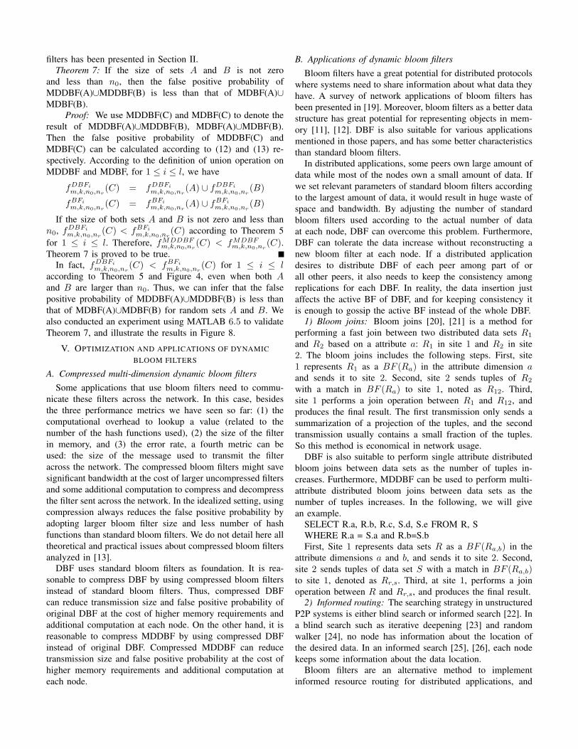
Fig. 8. False positive probability of MDBF(A)∪MDBF(B) minus that ofMDDBF(A)∪MDDBF(B) is a function of the size of set A and B wherem = 1280, k = 7, n0 = 133, and the attribute dimension of set A and Bare 3.

largest capacity is identical. For nr > n0, the false positiveprobability of MDBF is larger than that of MDDBF, we alsoillustrate this fact in Figure 7.

The false positive probability of MDDBF increases slowlywith nr, but the corresponding value of MDBF quicklyincreases to a high value, and then, slowly increases to almostone. We can infer from (12), (13), and Figure 7 that MDDBFscales better than MDBF when the actual set size exceeds thepredefined value.

C. Algebra operations on multi-dimension bloom filters

We assume that there are random dynamic sets A and Bwith identical attribute dimensions.

Definition 4: (Union of multi-dimension dynamic bloomfilters) Assume that sets A and B are represented as MD-DBF(A) and MDDBF(B) respectively. MDDBF(A)∪ MD-DBF(B) result in a new MDDBF(C), and the DBF of MD-DBF(C) for each attribute dimension equals to the union resulton DBF of MDDBF(A) and MDDBF(B) for the same attributedimension. The detailed union operation on DBF has beenpresented in Section III.

Theorem 6: The false positive probability of MDDBF(A)∪MDDBF(B) is larger than that of MDDBF(A) and MD-DBF(B).

Proof: We use MDDBF(C) to denote the result ofMDDBF(A)∪ MDDBF(B). For 1 ≤ i ≤ l, according to thedefinition of union operation on MDDBF, we can conclude thatfDBFi

m,k,n0,nr(C) = fDBFi

m,k,n0,nr(A)∪fDBFi

m,k,n0,nr(B). Furthermore,

it is easy to see that fDBFi

m,k,n0,nr(A) ∪ fDBFi

m,k,n0,nr(B) is larger

than fDBFi

m,k,n0,nr(A) and fDBFi

m,k,n0,nr(B) according to Theorem

4. We can infer that fDBFm,k,n0,nr

(C) is larger than fDBFm,k,n0,nr

(A)and fDBF

m,k,n0,nr(B). Theorem 6 is proved to be true.

Definition 5: (Union of multi-dimension bloom filters) Ifset A and B are represented as MDBF(A) and MDBF(B),the union of MDBF(A) and MDBF(B) will result in a newMDBF(C). The standard bloom filter of MDBF(C) for eachattribute dimension equals to the union result on standardbloom filters of MDBF(A) and MDBF(B) for the same at-tribute dimension. The union operation on standard bloom

filters has been presented in Section II.Theorem 7: If the size of sets A and B is not zero

and less than n0, then the false positive probability ofMDDBF(A)∪MDDBF(B) is less than that of MDBF(A)∪MDBF(B).

Proof: We use MDDBF(C) and MDBF(C) to denote theresult of MDDBF(A)∪MDDBF(B), MDBF(A)∪MDBF(B).Then the false positive probability of MDDBF(C) andMDBF(C) can be calculated according to (12) and (13) re-spectively. According to the definition of union operation onMDDBF and MDBF, for 1 ≤ i ≤ l, we have

fDBFi

m,k,n0,nr(C) = fDBFi

m,k,n0,nr(A) ∪ fDBFi

m,k,n0,nr(B)

fBFi

m,k,n0,nr(C) = fBFi

m,k,n0,nr(A) ∪ fBFi

m,k,n0,nr(B)

If the size of both sets A and B is not zero and less thann0, fDBFi

m,k,n0,nr(C) < fBFi

m,k,n0,nr(C) according to Theorem 5

for 1 ≤ i ≤ l. Therefore, fMDDBFm,k,n0,nr

(C) < fMDBFm,k,n0,nr

(C).Theorem 7 is proved to be true.

In fact, fDBFi

m,k,n0,nr(C) < fBFi

m,k,n0,nr(C) for 1 ≤ i ≤ l

according to Theorem 5 and Figure 4, even when both Aand B are larger than n0. Thus, we can infer that the falsepositive probability of MDDBF(A)∪MDDBF(B) is less thanthat of MDBF(A)∪MDBF(B) for random sets A and B. Wealso conducted an experiment using MATLAB 6.5 to validateTheorem 7, and illustrate the results in Figure 8.

V. OPTIMIZATION AND APPLICATIONS OF DYNAMIC

BLOOM FILTERS

A. Compressed multi-dimension dynamic bloom filters

Some applications that use bloom filters need to commu-nicate these filters across the network. In this case, besidesthe three performance metrics we have seen so far: (1) thecomputational overhead to lookup a value (related to thenumber of the hash functions used), (2) the size of the filterin memory, and (3) the error rate, a fourth metric can beused: the size of the message used to transmit the filteracross the network. The compressed bloom filters might savesignificant bandwidth at the cost of larger uncompressed filtersand some additional computation to compress and decompressthe filter sent across the network. In the idealized setting, usingcompression always reduces the false positive probability byadopting larger bloom filter size and less number of hashfunctions than standard bloom filters. We do not detail here alltheoretical and practical issues about compressed bloom filtersanalyzed in [13].

DBF uses standard bloom filters as foundation. It is rea-sonable to compress DBF by using compressed bloom filtersinstead of standard bloom filters. Thus, compressed DBFcan reduce transmission size and false positive probability oforiginal DBF at the cost of higher memory requirements andadditional computation at each node. On the other hand, it isreasonable to compress MDDBF by using compressed DBFinstead of original DBF. Compressed MDDBF can reducetransmission size and false positive probability at the cost ofhigher memory requirements and additional computation ateach node.

B. Applications of dynamic bloom filters

Bloom filters have a great potential for distributed protocolswhere systems need to share information about what data theyhave. A survey of network applications of bloom filters hasbeen presented in [19]. Moreover, bloom filters as a better datastructure has great potential for representing objects in mem-ory [11], [12]. DBF is also suitable for various applicationsmentioned in those papers, and has some better characteristicsthan standard bloom filters.

In distributed applications, some peers own large amount ofdata while most of the nodes own a small amount of data. Ifwe set relevant parameters of standard bloom filters accordingto the largest amount of data, it would result in huge waste ofspace and bandwidth. By adjusting the number of standardbloom filters used according to the actual number of dataat each node, DBF can overcome this problem. Furthermore,DBF can tolerate the data increase without reconstructing anew bloom filter at each node. If a distributed applicationdesires to distribute DBF of each peer among part of orall other peers, it also needs to keep the consistency amongreplications for each DBF. In reality, the data insertion justaffects the active BF of DBF, and for keeping consistency itis enough to gossip the active BF instead of the whole DBF.

1) Bloom joins: Bloom joins [20], [21] is a method forperforming a fast join between two distributed data sets R1

and R2 based on a attribute a: R1 in site 1 and R2 in site2. The bloom joins includes the following steps. First, site1 represents R1 as a BF (Ra) in the attribute dimension aand sends it to site 2. Second, site 2 sends tuples of R2

with a match in BF (Ra) to site 1, noted as R12. Third,site 1 performs a join operation between R1 and R12, andproduces the final result. The first transmission only sends asummarization of a projection of the tuples, and the secondtransmission usually contains a small fraction of the tuples.So this method is economical in network usage.

DBF is also suitable to perform single attribute distributedbloom joins between data sets as the number of tuples in-creases. Furthermore, MDDBF can be used to perform multi-attribute distributed bloom joins between data sets as thenumber of tuples increases. In the following, we will givean example.

SELECT R.a, R.b, R.c, S.d, S.e FROM R, SWHERE R.a = S.a and R.b=S.bFirst, Site 1 represents data sets R as a BF (Ra,b) in the

attribute dimensions a and b, and sends it to site 2. Second,site 2 sends tuples of data set S with a match in BF (Ra,b)to site 1, denoted as Rr,s. Third, at site 1, performs a joinoperation between R and Rr,s, and produces the final result.

2) Informed routing: The searching strategy in unstructuredP2P systems is either blind search or informed search [22]. Ina blind search such as iterative deepening [23] and randomwalker [24], no node has information about the location ofthe desired data. In an informed search [25], [26], each nodekeeps some information about the data location.

Bloom filters are an alternative method to implementinformed resource routing for distributed applications, and

many literatures have recently presented different approachesto utilize bloom filters for different scenarios [6], [7], [8],[9], [27]. The common assumption in those literatures is torepresent local resource using bloom filters and gossip it toother peers according to different control mechanisms. Thus,each peer can possess individual bloom filters coming fromrelated peers, then re-construct them according to the distanceand/or direction between the local peer and other peers, andobtain a set of union results of individual bloom filters at eachrelative distance and/or relative direction.

A dynamic bloom filter is still suitable to support informedrouting, and has more advantages than the standard one as theresource at each peer increases. Furthermore, a dynamic bloomfilter is more suitable to support the necessary union operationthan the standard one according to Theorem 5. As mentionedabove, dynamic bloom filters, standard bloom filters, andtheir variations just represent objects and support approximatemembership queries in a single attribute dimension. On theother hand, it often requires to route multi-attribute queries inreality. Both MDDBF and MDBF can satisfy this need. Theformer has the advantage over the latter as the resource ateach peer increases, and supports the union operation betterthan the latter according to Theorem 7. Thus, DBF and itsvariations are better alternatives than standard bloom filters toimplement informed routing in some scenarios.

3) Implementation of global index: We will refer to theglobally replicated index as the global index, while the moredetailed index that describes only the resources hosted locallyby a peer will be denoted as the local index. Global index canbe implemented in a number of ways. We define bloom filtersin such a way that each peer summarizes the set of terms in itslocal index as a bloom filter. The cost of replicating the globalindex can be reduced by simply decreasing the gossiping rate;updating the global index with a new bloom filter requiresconstant time, regardless of the number of changes introduced.Furthermore, bloom filters can be compressed to achieve a sin-gle bit per word average ratio. Memory-constrained peers canalso independently trade accuracy for storage by combiningseveral filters into one.

When the global index has been established and propagatedto the whole network, each peer uses a copy of global indexhosted at local storage to find the desired peers and appropriateresources within one hop. In order to support queries thatcontain a set of queries based on different attribute dimensions,we can adopt MDDBF to summarize local content index andconstruct global content index by a periodic gossiping updateoperation.

VI. SIMULATION

In this section, we present a simulation-based evaluationof the informed search protocol and compare its performancewith other blind search protocols.

We use PeerSim to design and implement our experimenta-tions. PeerSim is delivered by the BISON project [28], and isan open source, Java based, P2P simulation framework aimedto develop and test any kind of P2P algorithm in a dynamic

environment. It supports both cycle based and event basedsimulation. Our experiment is cycle based, which means thatthe simulation runs in a sequential order and in each cycleeach protocol can run its behavior independently. It is easyfor PeerSim to simulate more than one protocol in the samerunning context, and to compare many performance metricesbetween different protocols.

A. Informed search protocol based on bloom filters

Basically, the informed search protocol is a forward-basedrouting protocol. It has two major components, the construc-tion and maintenance of a routing table, and a query forwardmechanism using the routing table. In our informed protocol,the routing table is a set of dynamic bloom filters or multi-dimension dynamic bloom filters, each corresponding to alink. When a peer needs to forward a query, bloom filterscorresponding to each link will be scanned and desired linkswill be filtered out as the forwarding directions.

In order to construct a routing table, Kumar et al havepresented a novel method in [29]. Each peer first constructsthe local bloom filter and sends a routing advertisement (in theform of a dynamic or multi-dimension dynamic bloom filter)to the neighbor during a connection setup. Then, the neighborcan construct a routing entry for the link from itself to the newpeer. The initial advertisement is created by taking the decayunion of all advertisements received from neighbors other thanthe target neighbors and the union of local bloom filters. Itwould be better for the method in [29] to adopt the gossipingprotocol [30] to exchange advertisements between the sourceand sink peer instead of push or pull. The experiment showsthat the convergent speed of the gossiping protocol is fasterthan that of a single push protocol.

However, the mechanism in [29] alone is not enoughto ensure that each routing entry contains whole summaryinformation of the reachable data along the corresponding linkdirection. In fact, the majority of early arriving peers have littleinformation about the later peers, although the later peers haveenough information about the early peers. Thus, we shouldpay more attention to update the routing table. Kumar et alhave presented a push protocol in which each peer constructsand pushes the update advertisement for each neighbor duringa given interval. In our experiment, we found that it is notnecessary to update all link directions. We also adopt theasynchronous gossiping update protocol, and each peer createsan update advertisement for a random link direction at eachgossiping round, and exchanges update advertisements in thatdirection.

The query forward mechanism is tightly coupled with thebloom filter corresponding to each link. Before the bloom filterof a given peer has propagated through the whole P2P networkwithout any information loss, queries with payload containedby the peer may be issued at any time from any other peer.In reality, the search protocol may be designed to decay thebloom filter of a given peer during the propagation process inorder to save bandwidth and make the protocol more scalable,such as the protocol mentioned in [29].

0 0.1 0.2 0.3 0.4 0.5 0.6 0.7 0.8 0.90

0.1

0.2

0.3

0.4

0.5

0.6

0.7

0.8

0.9

1

The ratio of visited peers to total peers

Reca

ll

FloodingInformed Search

Fig. 9. The ratio of visited peers for one query to total peers vs. recall.

In order to overcome information uncertainty, we combinethe informed search protocol based on bloom filters with the krandom walker protocol. After a peer receives a query, it willprocess the query and check whether to terminate the query.If the check result is true, the peer does not forward the queryto any neighbor. Otherwise, the peer will forward the queryto part of or all neighbors selected according to its routingtable and Algorithm 2(or Algorithm 4). If there is no satisfiedneighbor, the k random walker will be used as the assistantquery forward protocol. This policy is also suitable when apeer initiates a query.

B. Simulation result analysis

In this section, we present simulation results usingGnutella0.4, k random walk, and informed search based onbloom filters in a random P2P network with 5,000 nodes.There are multiple replications of some objects at differentlocations. The model we use for replication of content isbased on the zipf distribution, frequently used to model thereplication of objects on the web. The ith most popularelementary object of a space will have 1/ia times as manyreplicas as the most replicated object. In our experiment, thesize of the entire object space is 50, 000, the size of elementaryobject space is 5, 000, and the parameter a used by the zipflaw is set to 0.5. The total number of queries is 10, 000, andthe distribution of query’s payload also obeys the zipf law, andthe parameter a is set to 0.5.

Performance issues in actual P2P networks are extremelycomplicated. In addition to issues such as load on the network,load on network participants, delay and success rate of query,there is a host of other metrices. In our experiment, we focuson efficiency aspects of algorithms, and use the followingsimple metrics.

• Pr(success): the probability of finding the queried objectbefore the search terminates. Different algorithms havedifferent criteria for terminating the search; it dependson the search semantics.

• Recall: the ratio of the number of relevant documentspresented to the user to the total number of relevantdocuments in the P2P network.

• Nodes visited: the number of peers that a query’s searchmessage travel through. This is an indirect measure of

0 0.02 0.04 0.06 0.08 0.1 0.12 0.140

0.1

0.2

0.3

0.4

0.5

0.6

0.7

0.8

0.9

1

The ratio of visited peers to total peers

% o

f que

ries

answ

ered

Random walkInformed search

Fig. 10. The ratio of visited peers to total peers vs. % of queries.

the impact that a query generates on the whole network.The simulation result of search for all copies (i.e., to get all

the copies of a given object) under protocol Gnutella0.4 andour informed search based on bloom filters is illustrated inFigure 9. For any query, informed search protocol can obtainhigh recall without visiting a large portion of the whole P2Pnetwork in order to process the query, while the Gnutella-likeprotocol can obtain relatively lower recall with the cost ofvisiting a large portion of the whole P2P network. It is shownthat the informed search based on bloom filters can avoid themessage flooding problem.

The simulation result of search for one copy (i.e., to getat least one copy of a given object) under the random walkerprotocol and our informed search based on bloom filters isillustrated in Figure 10. For any query, the informed searchprotocol can obtain high Pr(success) compared to randomwalker with the same ratio of visited peers in the wholenetwork. When there are multiple replications distributedrandomly among the whole P2P network for any object, thePr(success) of both protocols can almost reach 1 after visitingless than 10% of the whole network. It also explains thatinformed search based on bloom filters possesses advantagesover blind search.

The overhead of our informed search protocol is the needto exchange information between peers at a given gossipingrate. This operation can be merged with the stabilizationoperation, which is used to manage the neighbor relationshipand maintain the P2P network. Furthermore, the transitive sizecan become small by adopting bloom filters and compressedbloom filters.

VII. CONCLUSION

A bloom filter is a simple, space-efficient, randomized datastructure for concisely representing a static data set in orderto support approximate membership queries. As the actualsize of the set increases continuously after deployment, abloom filter should scale well in order to avoid too muchdeviation between the actual false positive probability andthe predefined threshold. In order to deal with this problem,we present dynamic bloom filters to support concise repre-sentation and approximate membership queries of dynamicsets. It has been proved that dynamic bloom filters not only

possess the advantage of standard bloom filters, but also havebetter features than standard bloom filters when dealing withdynamic sets. False positive probability of dynamic bloomfilters can be controlled at a low level, and space complexityis also acceptable if the estimation of the threshold of thedynamic set does not deviate too much. In addition, wepresent multi-dimension dynamic bloom filters to supportconcise representation and approximate membership queriesof dynamic sets from multiple attribute dimensions.

We have explored three kinds of representative applicationsof dynamic bloom filters: bloom joins, informed search, andimplementation of global index. These applications also illus-trate that dynamic bloom filters and their variations scale welland are practical for representing dynamic sets. Finally, wehave simulated the informed search protocol based on bloomfilters in unstructured P2P networks. Our simulation showsthat informed search based on bloom filters can obtain highrecall and success rate of query than the blind search protocol.

In future work, we will further enhance dynamic bloomfilters in order to support the removal operation, and comparethe space/time trade-off of both dynamic and standard bloomfilters.

ACKNOWLEDGMENT

The authors would like to thank Yongbo Wu for the helpto prove a theorem, Kang Chen for the help to design relatedexperiments, and Yang Ren and Yanli Hu for their constructivecomments.

REFERENCES

[1] B. Bloom. Space/time tradeoffs in hash coding with allowable errors.Commun. ACM, 13(7):422–426, 1970.

[2] J. K. Mullin. Optimal semijoins for distributed database systems. IEEETrans. Software Eng., 16(5):558–560, 1990.

[3] J. Kubiatowicz, D. Bindel, Y. Chen, S. Czerwinski, P. Eaton, andD. Geels. Oceanstore: An architecture for global-scale persistent storage.ACM SIGPLAN Notices.

[4] J. Li, J. Taylor, L. Serban, and M.Seltzer. Self-organization in peer-to-peer system. In Proc. the 10th ACM SIGOPS European Workshop,Saint-Emilion, France, September 2002.

[5] F. M. Cuena-Acuna, C. Peery, R. P. Martin, and T. D. Nguyen. Plantp:Using gossiping to build content addressable peer-to-peer informationsharing communities. In Proc. the 12th IEEE International Symposiumon High Performance Distributed Computing, pages 236–249, Seattle,WA, USA, June 2003.

[6] S. C. Rhea and J. Kubiatowicz. Probabilistic location and routing. InProc. IEEE INFOCOM, pages 1248–1257, New York, NY, United States,June 2004.

[7] T. D. Hodes, S. E. Czerwinski, and B. Y. Zhao. An architecture forsecure wide-area service discovery. Wireless Networks, 8(2-3):213–230,2002.

[8] P. Reynolds and A. Vahdat. Efficient peer-to-peer keyword searching.In Proc. ACM International Middleware Conference, pages 21–40, Riode Janeiro, Brazil, June 2003.

[9] D. Bauer, P. Hurley, R. Pletka, and M. Waldvogel. Bringing efficientadvanced queries to distributed hash tables. In Proc. IEEE Conferenceon Local Computer Networks, pages 6–14, Tampa, FL, United States,November 2004.

[10] L. Fan, P. Cao, J. Almeida, and A. Broder. Summary cache: A scalablewide-area web cache sharing protocol. IEEE/ACM Trans. Networking,8(3):281–293, 2000.

[11] C. Jin, W. Qian, and A. Zhou. Analysis and management of streamingdata: A survey. Journal of Software, 15(8):1172–1181, 2004.

[12] C. D. Peter and M. Panagiotis. Bloom filters in probabilistic verification.In Proc. the 5th International Conference on Formal Methods inComputer-Aided Design, pages 367–381, Austin, Texas, USA, Novem-ber 2004.

[13] M. Mitzenmacher. Compressed bloom filters. IEEE/ACM Trans.Networking, 10(5):604–612, 2002.

[14] A. Kirsch and M. Mitzenmacher. Distance-sensitive bloom fil-ters. http://www.eecs.harvard.edu/ michaelm/postscripts/lsbf.ps, January2006.

[15] A. Kirsch and M. Mitzenmacher. Building a better bloom filter.http://www.eecs.harvard.edu/ michaelm/postscripts/tr-02-05.pdf, January2006.

[16] A. Kumar, J. Xu, J. Wang, O. Spatschek, and L. Li. Space-codebloom filter for efficient per-flow traffic measurement. In Proc. IEEEINFOCOM, pages 1762–1773, Hongkong, China, March 2004.

[17] S. Cohen and Y. Matias. Spectral bloom filters. In Proc. ACMInternational Conference on Management of Data (SIGMOD), pages241–252, San Diego, CA, United States, June 2003.

[18] M. Xiao, Y. Dai, and X. Li. Split bloom filters. Chinese Journal ofElectronic, 32(2):241–245, 2004.

[19] A. Broder and M. Mitzenmacher. Network applications of bloom filters:A survey. Internet Mathematics, 1(4):485–509, 2005.

[20] L. F. Mackert and G. M. Lohman. R* optimizer validation andperformance evaluation for distributed queries. In Proc. the 12thInternational Conference on Very Large Data Bases (VLDB), pages 149–159, Kyoto, Jpn, August 1986.

[21] Z. Li and K. A. Ross. Perf join: An alternative to two-way semijoinand bloomjoin. In Proc. International Conference on Informationand Knowledge Management, pages 137–144, Baltimore, MD, USA,November 1995.

[22] X. Li and J. Wu. Searching techniques in peer-to-peer networks. InJ. Wu, editor, Handbook of Theoretical and Algorithmic Aspects of AdHoc, Sensor, and Peer-to-Peer Networks. Auerbach, New York,USA,2006.

[23] B. Yang and H. Garcia-Molina. Improving search in peer-to-peer net-works. In Proc. the 22th IEEE International Conference on DistributedComputing, pages 5–14, Vienna, Austria, July 2002.

[24] Q. Lv, P. Cao, E. Cohen, K. Li, and S. Shenker. Search and replication inunstructured peer-to-peer networks. In Proc. the 16th ACM InternationalConference on Supercomputing, pages 84–95, Marina Del Rey, CA,United States, June 2002.

[25] A. Crespo and H. Garcia-Molina. Routing indices for peer-to-peersystems. In Proc. the 22th International Conference on DistributedComputing, pages 23–32, Vienna, Austria, July 2002.

[26] D. Tsoumakos and N. Roussopoulos. Adaptive probabilistic search inpeer-to-peer networks. In Proc. the 3th International Conference onPeer-to-Peer Computing, pages 102–109, Sweden, September 2003.

[27] K. Shanmugasundaram, H. Bronnimann, and N. Memon. Payloadattribution via hierarchical bloom filters. In Proc. the 11th ACMConference on Computer and Communications Security, pages 31–41,Washington, DC, United States, October 2004.

[28] G. D. Caro, F. Ducatelle, P. Heegaard, M. Jelasity, R. Montemanni, andA. Montresor. Evaluation of basic services in ahn,p2p and grid networks.http://www.cs.unibo.it/bison/deliverables/D07.pdf, February 2005.

[29] A. Kumar, J. Xu, and E. W. Zegura. Effcient and scalable query routingfor unstructured peer-to-peer networks. In Proc. IEEE INFOCOM, pages1162–1173, Miami, FL, United States, March 2005.

[30] S. Boyd, A. Ghosh, B. Prabhakar, and D. Shah. Gossip algorithms:Design, analysis and applications. In Proc. IEEE INFOCOM, pages1653–1664, Miami, FL, United States, March 2005.