theoretical treatment of asphaltene gradients in the presence of gor gradients

3942r 2010 American Chemical Society pubs.acs.org/EF

Energy Fuels 2010, 24, 3942–3949 : DOI:10.1021/ef1001056Published on Web 06/03/2010

Theoretical Treatment of Asphaltene Gradients in the Presence of GOR Gradients

Denise E. Freed,*,† Oliver C. Mullins,† and Julian Y. Zuo‡

†Schlumberger-Doll Research, 1 Hampshire Street, Cambridge, Massachusetts 02139, and ‡DBR Technology Center,Schlumberger, 9450 17th Avenue, Edmonton, Canada T6N 1M9

Received January 28, 2010. Revised Manuscript Received May 10, 2010

The modeling of hydrocarbon fluids in oil-field reservoirs is essential for optimizing production. Inparticular, the often large compositional variations of reservoir crude oils must be understood andmodeled. The two most important chemical constituents that govern many chemical and physicalproperties of subsurface reservoir crude oils are the dissolved gas content, described by the gas-oil ratio(GOR), and the asphaltene content. The modeling of GOR variations of crude oils in reservoirs has beenpracticed routinely for many decades. However, proper modeling of the asphaltenes and/or heavy ends ofreservoir crude oils has been precluded because of the lack of understanding of the chemical and physicalproperties of asphaltenes in crude oils. Recently, the modified Yen model has codified advances inasphaltene science by providing a framework for understanding the molecular and colloidal structure ofasphaltenes in crude oils. Here, a thermodynamic model of asphaltenes in reservoir crude oils is developedthat can incorporate the modified Yen model and thus can be used to treat reservoir crude oils. Ourobjective is to analyze the distribution of reservoir fluids, in particular the asphaltenes. This deviates frommost previous studies of asphaltene thermodynamics, which were focused on the phase behavior ofasphaltenes. Here, compositional gradients of asphaltenes, as well as the GOR of reservoir crude oils, areanalyzed. Asphaltene gradients are shown to be strongly affected by both gravity and solubility. The lattereffect is heavily dependent on the dissolved gas content of the reservoir crude oil. Case studies are providedthat exhibit the power of this modeling.

Introduction

The two most important chemical constituents that governmany chemical andphysical properties of subsurface reservoircrude oils are the dissolved gas content, described as thegas-oil ratio (GOR), and the asphaltene content. For exam-ple, surface or sea floor facilities are built according to gas andliquidvolumetric handling.Flow rates are critically dependenton the fluid viscosity, which is a function of both the light-end(e.g., gases) and heavy-end (e.g., asphaltenes) contents of thecrude oil. Moreover, reservoir fluids can exhibit variation ofimportant chemical properties, especially the light- andheavy-end contents, from a variety ofmechanisms.1 These variationsmust be understood for the building of optimal productionstrategies.

In addition to reservoir fluid complexities, reservoirs gen-erally possess complex architecture. In particular, reservoirscan have (infrequent) large compartments or can consist ofnumerous small compartments. (A compartment must bepenetrated by a well to be drained.) That is, in extremedescriptions, reservoirs can be similar to a kitchen sponge thathas a connected porosity or similar to a spool of bubble wrapthat has many small individual compartments. Compartmen-talization or its inverse, reservoir connectivity, is the biggestproblem in almost all deepwater projects around the world.1

There are many mechanisms that can produce reservoir fluidvariability. Often this variation in the fluid can address com-partmentalization because different compartments are likely to

be filled with different fluids. If a stair-step discontinuous fluidproperty is found (in a single phase) in the reservoir, thencompartmentalization is often indicated.1 In contrast, contin-uous and monotonic trends of reservoir fluid properties oftenimply connectivity because they suggest that there is massivefluid flow across the reservoir. If the reservoir fluids areequilibrated, especially in the heavy ends, then reservoir con-nectivity is more strongly implied.1 This follows because themobilities of the heavy ends are very low, so equilibrated heavyends are not compatiblewith substantially restricted flow in thereservoir. Consequently, it becomes more important than everto model all components of reservoir fluids.

Modeling GOR in reservoir fluids has been performed fordecades using variants of the van der Waals equation of state[or cubic equations of state (EOS)]. These equations have beenvery useful for describing a variety of fluid parameters. Forexample, heuristics have been developed to indicate whenGOR gradients are expected.2 In large measure, in compres-sible fluids, the greater expansion of the lightest componentsas they go higher in the columnwill create the thermodynamicdrive to give GOR gradients. In contrast, incompressiblefluids do not yield density variations and thus do not yieldGOR gradients.1,2 The success of cubic EOS to predict GORgradients in reservoir crude oils has been confirmed in livecrude oil centrifugation experiments.3 (Live crude oils arethose oils that, under reservoir pressure and temperatureconditions, contain dissolved gases.) However, treating solids,such as asphaltenes, as a pseudocomponent in a gas-liquid

*To whom correspondence should be addressed. E-mail: [email protected].(1) Mullins, O. C. The Physics of Reservoir Fluids; Discovery through

Downhole Fluid Analysis; Schlumberger Press: Houston, TX, 2008.

(2) Hoier, L.; Whitson, C. SPEREE 2001, 4, 525–535.(3) Ratulowski, J.; Fuex,A.N.;Westrich, J. T.; Sieler, J. J.Theoretical

and experimental investigation of isothermal compositional grading; SPE8477; SPE: Dallas, TX, 2003.

3943

Energy Fuels 2010, 24, 3942–3949 : DOI:10.1021/ef1001056 Freed et al.

equilibrium is not proper but has been used. Inappropriatemodeling of this nature might fit data, but it is far from pre-dictive for asphaltene gradients when compared to methodsbelow.

A new technology, “downhole fluid analysis” (DFA), hasenabled the determination of complex reservoir fluid gradi-ents in a cost-effective manner.1 DFA consists of sendingoptical spectrometers and other fluid sensors into oil wells,extracting reservoir fluids at known depths under controlledconditions, and performing chemical analysis of these livecrude oils.1 DFAhas had immediate application for measure-ment of the GOR gradients in the reservoir.4 The use of EOSto analyze corresponding gradients has also been successful.5

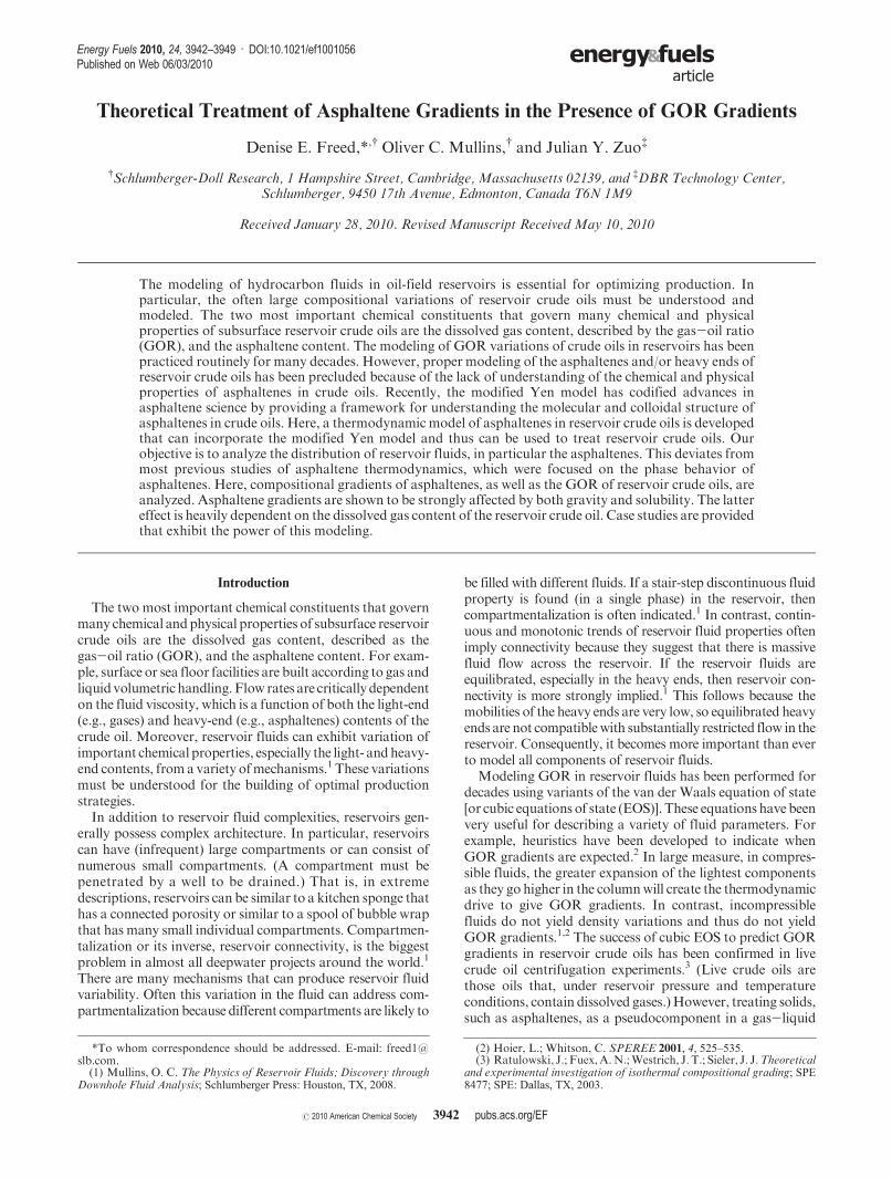
There has been a fundamental deficiency in analyzingreservoir fluids that has gone unsolved for decades and thathas been rooted in uncertainties in asphaltene science.6 Theasphaltenes could not be treated in any first principles model-ing effort because the aggregation state of asphaltenes in livecrude oils had been unknown. In addition, the asphaltenemolecular architecture had been unknown, and even theasphaltene molecular weight had previously been the subjectof an orders-of-magnitude debate.6 Without knowing themolecular and colloidal properties of asphaltenes, there isno way to properly handle the gravity effects in an EOS forheavy ends; consequently, they cannot be properly modeled.The magnitude of this inability to model asphaltenes is depic-ted in Figure 1, where 24 sample bottles of dead (degassed)crude oils from a single reservoir oil column are shown.7 Thisfigure shows that enormous variations in the concentration ofasphaltenes can occur in a single oil column, from0% to 5%.8

However, there was no ability to model this variation with anEOS. As a result, virtually all advanced reservoir modelsincorporate cubic EOS to treat (dissolved) gas and liquidhydrocarbons, but almost none of these reservoir models in-corporate any treatment for gradients of asphaltenes.Moreover,

because themagnitude of the asphaltene gradients can vary by afactor of 50, as determined in field studies,9 it is essential tounderstand and model these gradients.

Fortunately, there have been recent advances in asphaltenescience that have resolved molecular and colloidal structuresof asphaltenes, at least in crude oils that flow. These advances,described in detail elsewhere,6 are enabling a first-principlesapproach tomodeling asphaltenes. They are codified in a newparadigm of asphaltenes, the “modified Yen model”.10 Thismodel provides a framework for understanding the disper-sion of asphaltenes in crudeoil. In addition, it has found appli-cation in oil-field case studies and, using the theoreticalapproach in this paper, has successfully addressed some ofthe largest risk factors for the reservoir.9-13

The modified Yen model clarifies what the relevant struc-tures of asphaltenes in reservoir crude oils are, as shown inFigure 2. Because the effects of gravity on the asphaltenesdepend on the size of the asphaltene particles, this modelenables the treatment of asphaltenes and asphaltene gradientsin the reservoir. At very low concentrations, colored heavyends should be molecularly dispersed (either asphaltene orcolored resins). At higher asphaltene concentrations, the largerspecies are present. For example, in stable “black” crude oils(black crude oils have a relatively low GOR), the asphaltenenanoaggregates dominate.10 With increasing concentrationsand with weaker liquid-phase solvation, asphaltene nano-aggregate clusters can appear.10 Presumably, at much higherasphaltene concentrations, large asphaltene species will form.However, this is of lesser interest here because many of thesevery asphaltic crude oils will not flow and thus cannot beproduced conventionally. It must be emphasized that, fre-quently, only one particular form of asphaltenes is found inreservoir crude oil, such as asphaltene nanoaggregates in blackoil.9 This is in contrast tomany ad hoc asphaltene analyses thatassume changing asphaltene structures with depth.

Previous theoretical treatment of the asphaltene propertieshas focused on the phase behavior,14 particularly within a“flow assurance” context, and relates to colloidal destabilization

Figure 1. Samples of dead (degassed) crude oils from a single oil column.7 The color variation of these samples is caused primarily by differingasphaltene contents. In the past, this variation could not be modeled.

(4) Fujisawa, G.; Betancourt, S. S.; Mullins, O. C.; Torgersen, T.;O’Keefe, M.; Dong, C.; Eriksen, K. O. Large Hydrocarbon Composi-tional Gradient Revealed by In-Situ Optical Spectroscopy; SPE 89704;ATCE: Houston, TX, 2004.(5) Dubost, F. X.; Carnegie, A. J.; Mullins, O. C.; O’Keefe, M.;

Betancourt, S. S.; Zuo, J. Y.; Eriksen, K. O. Integration of In-Situ FluidMeasurements for Pressure Gradients Calculations; SPE 108494; Interna-tional Oil Conference Ex.: Veracruz, Mexico, 2007.(6) Asphaltenes, Heavy Oils and Petroleomics; Mullins, O., Hammami,

A., Marshall, A. G., Eds.; Springer: New York, 2007.(7) Elshahawi, H. (Shell Exploration and Production Company,

Houston, TX). Private communication,(8) Elshahawi,H.;Dong,C.;Mullins,O.C.;Hows,M.;Venkataramanan,

L.; McKinney, D.; Flannery, M.; Hashem, M. Integration of Geochemical,Mud Gas and Downhole Fluid Analysis for the Assessment of CompositionalGrading;Case Studies; SPE 109684; ATCE: Anaheim, CA, 2007.(9) Mullins, O. C.; Zuo, J. Y.; Freed, D. E.; Elshahawi, H.; Cribbs,

M. E.; Mishra, V. K.; Gisolf, A. Downhole Fluid Analysis Coupled withNovel Asphaltene Science for Reservoir Evaluation; SPWLA: Perth,Australia, 2010.

(10) Mullins, O. C. Energy Fuels 2010, 24, 2179–2207.(11) Pomerantz,A.E.; Ventura,G. T.;McKenna,A.M.;Canas, J.A.;

Auman, J.; Koerner, K.; Curry, D.; Nelson, R. K.; Reddy, C. M.;Marshall, A. G.; Mullins, O. C. Combining Bulk Biomarker and BulkCompositional Gradient Analysis to Assess Reservoir Connectivity.Submitted to J. Org. Geochem. 2010.

(12) Betancourt, S. S.; Ventura, G. T.; Pomerantz, A. E.; Viloria, O.;Dubost, F. X.; Zuo, J. Y.; Monson, G.; Bustamante, D.; Purcell, J. M.;Nelson, R. K.; Rodgers, R. P.; Reddy, C. M.; Marshall, A. G.; Mullins,O. C. Energy Fuels 2009, 23, 1178–1188.

(13) Mullins, O. C.; Betancourt, S. S.; Cribbs, M. E.; Creek, J. L.;Andrews, B. A.; Dubost, F.; Venkataramanan, L.Energy Fuels 2007, 21,2785–2794.

(14) Hammami, A.; Ratulowski, J. Precipitation and deposition ofasphlatenes in production systems: a flow assurance overview. InAsphaltenes, Heavy Oils and Petroleomics; Mullins, O. C., Sheu, E. Y.,Hammami, A., Marshall, A. G., Eds.; Springer: NewYork, 2007; Chapter 23.

3944


of asphaltenes, leading to solids deposition in pipelines, produc-tion tubing, and even the reservoir.15 This successful treatmentcontains elements that are quite useful for developing a moregeneralized treatment of asphaltenes that properly incorporatesthe effects of gravity. The approach we will describe herein hasbeenused to successfully treat the results fromcentrifugationofalive black crude oil.16

In this paper, a thermodynamic model is developed todescribe asphaltene distributions in reservoir crude oils. Threeterms are explicitly developed: gravity, solubility, and entropy.The solubility term is shown to depend heavily on the GOR ofthe crude oil and its variation with depth; thus, the light- andheavy-end treatments are intimately related. The relationshipof this formalism with the previous phase behavior work isdiscussed. An oil-field case study is shown where the gravityterm dominates, and a second field case study is shown wherethe solubility term dominates. The methods described here,coupled with the foundations of the modified Yen model,provide new powerful methods for addressing the complexitiesof reservoir crude oils.

Thermodynamic Model

Wewill use a simple, two-component, Flory-Huggins typeofmodel to describe the asphaltene andmaltene system. Basicmodeling of asphaltenes in reservoir crude oils has been des-cribed previously.17 However, this early work suffered fromtwo fundamental limitations: (1) at the time, there was nounderstanding of the molecular and colloidal structure ofcrude oil, which precluded the proper understanding of thegravity effects, and (2) possible GOR variations were notincluded, which precluded any consideration of the effects ofthe changing solubility. Here, we overcome both limitations.In our case, the amount of methane, and possibly othercomponents of the maltene, varies as a function of the height.

We extend the two-component Flory-Huggins model thathas been used to desribe the phase behavior of asphaltenes.15,18

In this model, the asphaltenes are the first component, and the

rest of the oil, or themaltene, is lumped together for the secondcomponent. In the case considered here, the properties of themaltene, such as its molar volume andmolar mass, can vary asa function of the height, but we assume that the properties ofthe asphaltene are independent of the height. We will alsoassume that the concentrationof the asphaltene is small enoughthat it does not affect the equilibrium distribution of the rest ofthe oil. We will take this equilibrium distribution as a givenproperty of the oil and see how it affects the equilibriumdistribution of the asphaltene.

The size of the relevant asphaltene particle can be chosendependingon thenatureof the crudeoil.This hasbeen shown tobe applicable to reservoir crude oils.10 Here, we do not modifythe asphaltene solubility parameter as a function of its colloidalormoleculardispersion. If therewere sufficient data tomotivatethis, our approach could incorporate this complication.

More specifically, at each height h, there are nm(h) maltenemolecules and na(h) asphaltene molecules. These numbersare allowed to vary in order to find the minimum of the freeenergy. The average volume of a maltene molecule is vm(h).This can vary somewhat as a function of h as the compositionand density of the maltene change. The asphaltenes can be insingle molecules, nanoaggregates, or nanoaggregate clusters.In this paper, we will assign all of the asphaltenes to be in onlyone of these three forms. This assumption can be relaxed infuture treatments, especially if motivated by more oil-fielddata. We will take va to be the average size of the asphalteneparticles in the fluid, andwewill assume that it is constant as afunction of height. The total volume of the fluid at each heightisVT(h)= vmnmþ vana. Unlike in the calculations of the onsetof asphaltene instability, we will be assuming that the fluidremains a single phase or stable colloidal dispersion at allheights.Thus, there is only one volumeof the single phase, andwewill takeVT (h) to be constant as a function of the moles ofasphaltenes and solvent. (We note that in many of the cal-culations of the effect of gravity, including those in ref 17, theenergy is calculated as a function of the pressure and tem-perature. Here, instead we are calculating it as a function ofthe volume and temperature, and we hold the volume fixed ateach height. Thus, strictly speaking, the energy ΔG definedbelow is really theHelmoltz free energy,ΔA. In this case, giventhe way we define the chemical potential below, we do notneed to explicitly include a term of the form Fvagh, where F isthe average density at height h. This term arises in our casebecause of the constraint of constant volume.)

Figure 2. Asphaltene structures per the modified Yen model:10 (left) the predominant asphaltene molecular architecture; (center) asphaltenenanoaggregates consisting of about sixmolecules; (right) asphaltene clusters consisting of about seven nanoaggregates. The specific asphaltenespecies that is present in a reservoir crude oil is dependent on the concentration, liquid-phase solubility parameter, and other conditions.

(15) Buckley, J. S.; Wang, X.; Creek, J. L. Solubility of the Least-Soluble Asphaltenes. In Asphaltenes, Heavy Oils and Petroleomics;Mullins, O. C., Sheu, E. Y., Hammami, A., Marshall, A. G., Eds.; Springer:New York, 2007; Chapter 16.(16) Indo,K.; Ratulowski, J.; Dindoruk, B.; Gao, J.; Zuo, J.;Mullins,

O. C. Energy Fuels 2009, 23, 4460–4469.(17) Hirschberg, A. J. Pet. Technol. 1988, 40, 89–94.(18) Hirschberg, A.; DeJong, L. N. J.; Schipper, B.; Meijer, J. SPE J.

1984, 24, 283–293.

3945


The volume fractions of themaltene and asphaltene at eachheight are given by φm(h) = vmnm/VT and φa(h) = vana/VT,respectively, and they sum to 1:

φmðhÞþφaðhÞ ¼ 1 ð1ÞThe solubility parameter of the asphaltene is δa, and the

solubility parameter of the maltenes, δm(h), depends on thecomposition and density of the maltene at each height.

The free energy at height h for the asphaltene and solvent oilis given by

ΔGðhÞ ¼ ΔGentropyðhÞþΔGsolðhÞþΔGgravðhÞ ð2Þwhere ΔGentropy(h) is the free energy due to the entropy ofmixing, ΔGsol(h) is the free energy due to the solubility of theasphaltene in the maltene, andΔGgrav is the free energy due togravity. When the difference in sizes between the solute andsolvent is not taken into account, the entropy of mixing isgiven by

ΔGentropyðhÞ ¼ kT ½nmðhÞ ln xmðhÞþ naðhÞ ln xaðhÞ� ð3Þwhere xm(h) and xa(h) are the mole fractions of the malteneand asphaltene, respectively. Once there is a difference in sizebetween the solute and solvent, several different values for theentropy of mixing have been used, including the one givenabove for molecules of equal size. Alternatively, for asphal-tene phase behavior, the Flory-Huggins entropy expressionfor polymer solutions has been used successfully;15 we use thishere. It is given by

ΔGentropy ¼ kTðnm ln φm þ na ln φaÞ ð4ÞBecause this form of the entropy depends largely on thevolume fraction of the asphaltenes, the exact molecular orcolloidal dispersion of the asphaltenes in the crude oil hasa much smaller effect on the asphaltene gradient than if theentropy term depended solely on the mole fractions of thedifferent asphaltene species.

The part of the free energy due to the solubility of theasphaltenes is given by

ΔGsol ¼ nmðhÞ φaðhÞ vmðhÞ ½δa -δmðhÞ�2 ð5ÞThe solubility term is independent of the type of colloidaldispersion of the asphaltenes provided that the asphaltenesolubility parameter also does not depend on this. The freeenergy due to gravity is given by

ΔGgravðhÞ ¼ g½nmðhÞ vmðhÞZ h

0

Fmðh0Þ dh0 þ naðhÞvaFah� ð6Þ

where Fa and Fm are the densities of the asphaltene andmaltene, respectively. The density of asphaltene solutions isimpacted very little by the aggregation state of the asphalteneat a given mass fraction.19 Because the density and averagevolume per molecule is changing in this simplified model forthe maltene, there is some ambiguity in defining the gravita-tional free energy of themaltene. Because the density does notvarymuch in the examples considered below, there are severalchoices thatwe couldmake for this term,which all give similaranswers, as long as we require this term to depend only onthe relative height and not on the absolute height.Here, we areusing the work tomove a volume element of size v(h) from thereference height h = 0 to the height h to calculate this freeenergy. We assume that the density of this volume element

changes as a function of height, so that it equals the density ofthe maltene at each height.

Because the sum of the asphaltene and maltene volumefractions at each height is equal to 1, we can eliminate φm andnm from the expression for the free energy to obtain

ΔGðhÞ ¼ kT na ln φa þVT

vm-nava

vm

� �lnð1-φaÞ

" #

þ navað1-φaÞðδa -δmÞ2 þ gnava½Fah-Z h

0

Fmðh0Þ dh0�

þ gVT

Z h

0

Fmðh0Þ dh0 ð7Þ

The chemical potential of the asphaltene at height h is then thederivative of ΔG(h) with respect to na with VT (h) held fixedat each height:

μaðhÞ ¼ kT ln φa -va

vmlnð1-φaÞþ 1-

va

vm

� �

þð1- 2φaÞvaðδa -δmÞ2 þ gva½Fah-Z h

0

Fmðh0Þ dh0� ð8Þ

In equilibrium, the derivative of ΔG with respect to na(h)equals zero, with the constraint that

Phna(h) equals the total

number of asphaltene molecules. Using a Lagrangemultiplierλ to enforce this constraint, we have

DΔGðhÞDnaðhÞ ¼ D

DnaðhÞ�λXh

naðhÞ�

ð9Þ

which gives

μaðhÞ ¼ λ ð10Þfor all heights h. Thus, the condition for equilibrium is thatthe chemical potentials for the asphaltene are the same at allheights, so that

μaðh1Þ ¼ μaðh2Þ ð11ÞSetting the chemical potentials at heights h1 and h2 equal, wefind

φaðh1Þφaðh2Þ

φmðh2Þφmðh1Þ

� �va=vm

¼ expf- ½Gravðh1, h2ÞþEntðh1, h2Þ

þSolðh1, h2Þ�=kTg ð12ÞIn this equation,Grav(h1,h2), Ent(h1,h2), andSol(h1,h2) are thecontributions to the chemical potential due to gravity, en-tropy, and solubility, respectively. The gravity term is given by

Gravðh1, h2Þ ¼ vag

� Z h1

0

ΔFðhÞ dh-Z h2

0

ΔFðhÞ dh�

ð13Þ

where ΔF(h) = Fa - Fm(h). The entropy term is given by

Entðh1, h2Þ ¼ kTva1

vmðh2Þ-1

vmðh1Þ� �

ð14Þ

and the solubility term is

Solðh1, h2Þ ¼ vaf½1- 2φaðh1Þ�½δa - δmðh1Þ�2

- ½1- 2φaðh2Þ�½δa -δmðh2Þ�2g ð15ÞIf the expression for the entropy in eq 3 is used instead of theFlory-Huggins version, then the left-hand side of eq 12,which comes from the entropy, gets modified. The volumefractions are replaced bymole fractions, and the ratio va/vm in

(19) Andreatta, G.; Bostrom, N.; Mullins, O. C. Langmuir 2005, 21,2728.

3946


the exponent is replaced by 1. In addition, there is no entropyterm in the exponent on the right-hand side of eq 12. Thisentropy term is, in effect, an excess entropy due to use ofthe Flory-Huggins entropy instead of the ideal gas entropyof eq 3.

When the asphaltene volume fraction is much less than 1,eq 12 becomes

φaðh1Þφaðh2Þ

¼ expf- ½Gravðh1, h2ÞþEntðh1, h2Þþ Solðh1, h2Þ�=kTg

ð16Þwhere now the solubility term is given by

Solðh1, h2Þ ¼ vaf½δa - δmðh1Þ�2 - ½δa - δmðh2Þ�2g ð17Þ

If, in addition, the composition of the solvent oil does notchange as a function of the height, then this reduces to thefamiliar expression

naðh1Þnaðh2Þ ¼ e- vagðh1 - h2ÞΔF=kT ð18Þ

Comparison with Data and the Relative Sizes of the

Different Energies

In this section,we examine two extreme cases in terms of therelative magnitude of the gravity, solubility, and entropyeffects. A total of six case studies have been published else-where using the modified Yen model.9,11,12 In addition, thistheoretical model, coupled with the modified Yen model,successfully accounted for centrifugation data of a black oilof moderate GOR where the asphaltene concentration variedby a factor of 10 and the colored resins varied by a factor of2.16Ourobjective here is toprovide support for our theoreticalapproach but not to do an exhaustive analysis of case studies.Moreover, because these case studies cost roughly $0.5 billioneach and takemany years, it takes a while to accumulate largenumbers of case studies.

In the first case considered here, the Tahiti reservoir isexamined. In this reservoir, the GOR is quite low. Conse-quently, the GOR gradient is very small and the asphaltenegradient is dominated by the gravity term. This oil has anAPIgravity of 28 and contains several percent of asphaltene. In thesecond case, the fluid is a near-critical fluid that exhibits alarge GOR gradient. This oil has an API gravity of 35. Thecolored heavy ends in this case are dominated by colored resinmolecules instead of asphaltenes, so they are largely molecu-larly dispersed. The large GOR gradient produces a largesolubility contrast, whereas the small (molecular) size reducesthe magnitude of the gravity term. Consequently, with thenear-critical fluid, the heavy-end gradient is dominated by thesolubility term.

There has been a general misunderstanding as to the originof GOR gradients with respect to gravity, so we address thisissue here. Crude oils with low GOR are rather incompres-sible, in contrast to high-GOR crude oils. If a crude oil has nocompressibility, then the hydrostatic head pressure of thecrude oil column does not give rise to a density gradient.(The hydrostatic head pressure at any point is the pressureexerted by the height of the oil column above that point; thispressure is, in addition to the ambient pressure, at the top ofthe reservoir.) Equation 18 can then be used to give the GORgradient that is directly due to the gravity term. By substitut-ing reasonable parametric values into eq 18, one finds that a

factor of 2 decrease in the methane content in the crude oiloccurs in a height of roughly 100 km. In other words, thegravity term in eq 18 alone does not yield any significantGORgradient. Instead, the GOR gradient induced by gravity is viacompressibility. If the fluid is compressible, then it will beenergetically favorable for the lightest components (which arealso the most compressible) to be on top. This is becausehigher in the reservoir the hydrostatic head pressure will beless, causing the fluid to expand. The light components willexpand more, so the gravitational energy will be reduced themost if they collect toward the top. Thus, the fluid will havelower density andmoremethane at the top of the column andhigher density and less methane at the base of the column. Inaddition, once there is separation due to this combination ofcompressibility and gravity, the solubility effects will enhancethe compositional variation.

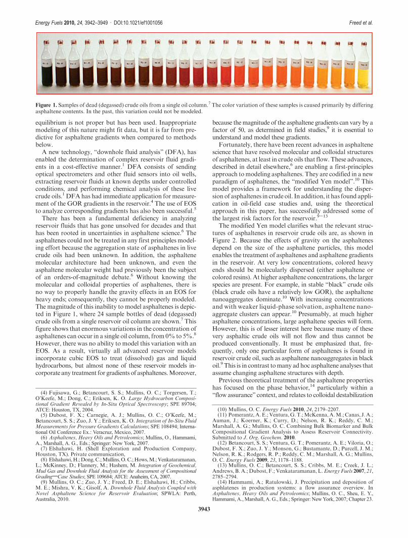
In the Tahiti reservoir, the crude oil GORs are relativelylow, ∼100 m3/m3. Consequently, there is a small GOR gra-dient, and variation of the solubility term in the 1000 m oilcolumn is relatively small. The gravity term (eq 18) actingdirectly on the colloidal asphaltene nanoaggregates is largelyresponsible for producing the asphaltene concentration gra-dient. Figure 3 shows theDFA-measured asphaltene gradientin the Tahiti reservoir.1,13 The coloration as measured byDFA at a specific, convenient wavelength has been shown tobe linear in the asphaltene content, with a small offset at theorigin due to some coloration of the resin fraction.1,13 Inaddition, it has been established that aggregation of asphal-tenes does not affect the asphaltene optical density associatedwith electronic transitions.20 Thus, no nonlinearties are in-troduced relating the asphaltene concentration and opticalabsorption.20 The asphaltene gradient in Figure 3 is consis-tent with a nanoaggregate distribution of asphaltenes in thecrude oil.1,13 That is, there is only one (centroid) size of theasphaltene particles throughout the entire oil column.There is

Figure 3.Asphaltene gradient (linear in optical density at 1000 nm)versus depth in the Tahiti reservoir. The gradient is predominantlydue to gravity acting on the asphaltene nanaoggregates.1,13 There isa small GOR gradient and low GOR so the solubility term isrelatively small. The solid lines show the fits using gravity effects(eq 18).

(20) Ruiz-Morales, Y.; Wu, X.; Mullins, O. C. Energy Fuels 2007, 21,944.

3947


not a changing distribution of sizes with the height in thecolumn. Similarly, a heavy oil column has recently beenshown to consist of clusters.9 Again, only a single size of theasphaltene particle is found in that case.

In the original Tahiti study, the effects of solubility andentropy were not included because it was assumed that thepredominant effect was from gravity. By fitting just thegravity term (eq 18) to the data, the asphaltene nanoaggregatediameter was found to be about 1.6 nm. If we include thesolubility term (assuming a solubility parameter of 21.85MPa1/2), this is decreased slightly to about 1.5 nm, and ifboth the solubility and entropy terms are included (as ineq 16), it is increased to about 1.8 nm. Thus, the solubilityterm does have a very small effect on the compositionalgradient and tends to increase it. The entropy term has asomewhat larger effect. Although the change is small, thelarger value for the asphaltene diameter found by includingthe solubility and entropy effects is more physical and moreconsistent with laboratory data for asphaltene nano-aggregates10 than the value found using only the gravity term.We also note that, although the oil column is quite long, thetemperature gradient was fairly small (about 0.01 K/m), andan analysis taking into account the gravity effects along withthe temperature gradient gave very similar results. Finally, weemphasize that we have used very few parameters to char-acterize the asphaltenes and that these parameters have beenmeasured in the laboratory, allowingour theoretical approachto be validated against specific known parameters.

Next, we contrast the Tahiti case study, where gravitydominates, with the Norway case study, where the solubilityterm dominates. Figure 4 shows the GOR gradient obtainedbyDFA in awell for both the Tahiti andNorway case studies.As can be seen in the figure, the Norway reservoir has a largeGOR variation over a range of only 30 m, while the Tahitireservoir has a much smaller variation of the GOR over amuch larger oil column spanning 1000m. Thus, not only doesthe Norway oil have a higher GOR than the Tahiti oil, it alsohas much larger gradients in the GOR. As we shall see below,this will cause the solubility effects to dominate the asphaltenegradient.

In the Norway well, the oil is very close to its critical point,so variations in the oil properties, including the GOR andoptical density, are significant, as described elsewhere.1,4,5 Forthis light oil, we expect the colored component to be moreresinlike and thus molecularly dispersed. In particular, theresins and this oil absorb light only at shorter wavelengths.16

For condensates, where asphaltenes have very poor solubility,such as this Norway example, optical obsorption occurs atshort wavelengths. Thus, the bulk of the absorption is ex-pected from molecularly dispersed species. Here, we employour thermodynamicmodel on the colored resinmolecules. It isknown that the colored resinmolecular size is similar to that ofasphaltene molecules with similar spectral characteristics.21

For this condensate, we use the DFA visible color mea-surement at λ = 647 nm for determination of the colored(asphaltene-like) resin content.

To simulate the pressure-volume-temperature (PVT)properties and compositions of the oil as a function of the

depth, the Peng-Robinson EOS and characterization proce-dure of Zuo et al.22 was used. The measured composition ofthe fluid froma region close to the gas-oil contactwas used asa reference point. The EOS was applied to estimate the molarvolume, density, and solubility of the maltene. The values ofthese parameters are shown in Figure 5. The linear fits, shownwith solid lines in the figures, are used in the calculationsbelow.

For purposes of fitting the data, we assume that theasphaltene has a solubility parameter of 21.85 MPa1/2 for anasphaltene sample at 20 �C.23 For the condensate, the coloredcomponent is probably more resin-like, in which case thesolubility parameter could be somewhat lower. The solubilityparameter could also be affected by the temperature andpressure, as will be discussed in the next section.

Figure 4. GOR variations of the reservoir crude oils for the Tahitireservoir (squares) and the Norway reservoir (circles). For theTahiti reservoir, this GOR variation occurs over an oil columnheight of 1000 m (left ordinate), while for the Norway reservoir, theGOR variation is for an oil column height of 30 m (right ordinate).The GOR gradient of the Norway oil field is much larger; conse-quently, the impact of the solubility term on the asphaltene gradientis huge. For the Tahiti oil field, the GOR gradient is very small;consequently, the gravity term dominates the asphaltene gradient.

Figure 5.Maltene properties for the Norway crude oil versus depth:(left) maltene molar volume vs depth; (middle) maltene density vsdepth; (right) maltene solubility parameter vs depth.

(21) Groenzin, H.; Mullins, O. C. Energy Fuels 2000, 14, 677.(22) Zuo, J. Y.; Freed, D. E.; Mullins, O. C.; Zhang, D.; Gisolf, A.

Interpretation of DFA Color Gradients in Oil Columns Using theFlory-Huggins Solubility Model. Paper SPE 130305 presented at theCPS/SPE International Oil and Gas Conference and Exhibition inChina, Beijing, China, June 8-10, 2010.

(23) Ting, P. D.; Hirasaki, G. J.; Chapman, W. G. Pet. Sci. Technol.2003, 21, 647–661.

3948


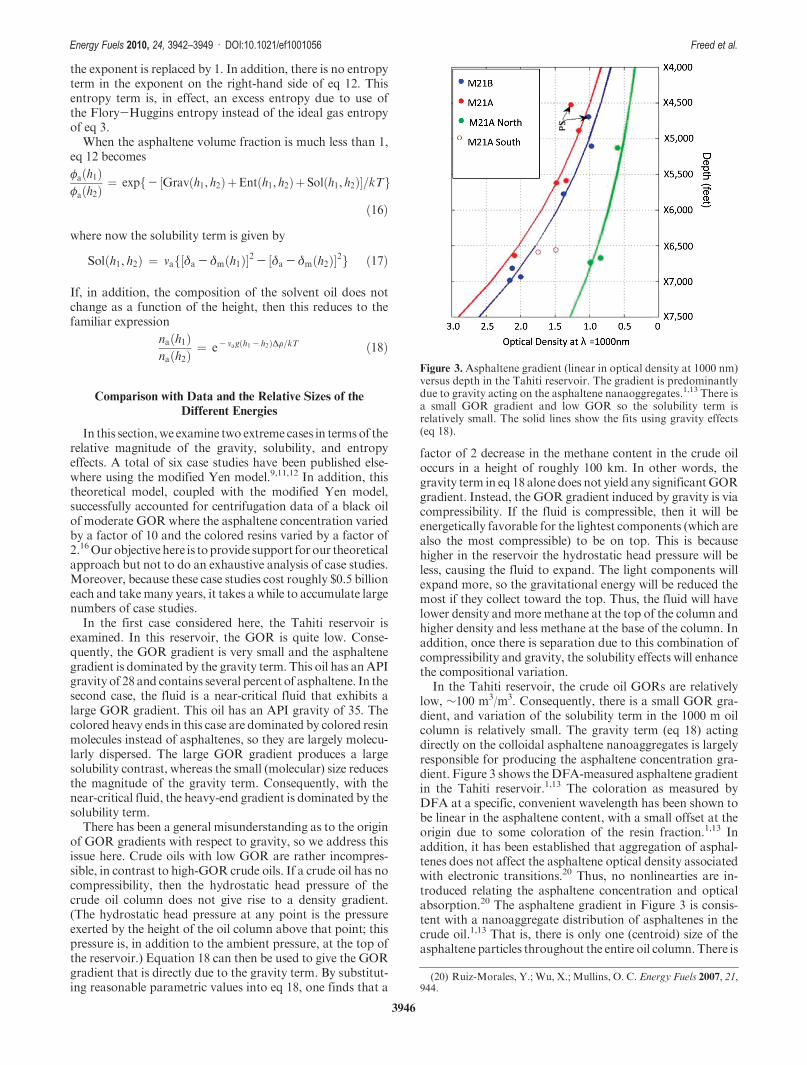
Next, we use all three terms, gravity, solubility, and en-tropy, to analyze the observed heavy-end gradients in the oilcolumn. Figure 6 shows themeasured coloration profile in thecondensate oil column, asmeasured byDFA. In addition, fitsto the theory are also shown. The solid line shows the fit usingthe gravity, solubility, and entropy terms, while the dashedline shows the fits with just the gravity and solubility terms.

For the fits in Figure 6, the size of the colored resinmoleculeis the only fitting parameter. With the value of 21.85 MPa1/2

for the solubility parameter, we find that the (hard-sphere)diameter of the asphaltene particles is 1.28 nm, which iscomparable to known measured diameters of colored resinmolecules.21 The large GOR gradient (cf. Figure 4) creates alarge gradient in the solubility parameter of the condensate.In turn, this creates and dominates the large gradient of thecolored resins. If the entropy term is neglected, then thediameter of colored resin size is reduced slightly (d=1.18nm). Essentially, entropy acts to create a more homogeneouscolumn. Thus, a somewhat larger gravity term is needed toproduce the same gradient. For this condensate, ignoring thelarge solubility termwould give an unphysical size of 4 nm forthe resin molecule. This is in contrast to the Tahiti case, whereincluding the entropy and solubility terms changed the dia-meter by only a small amount.

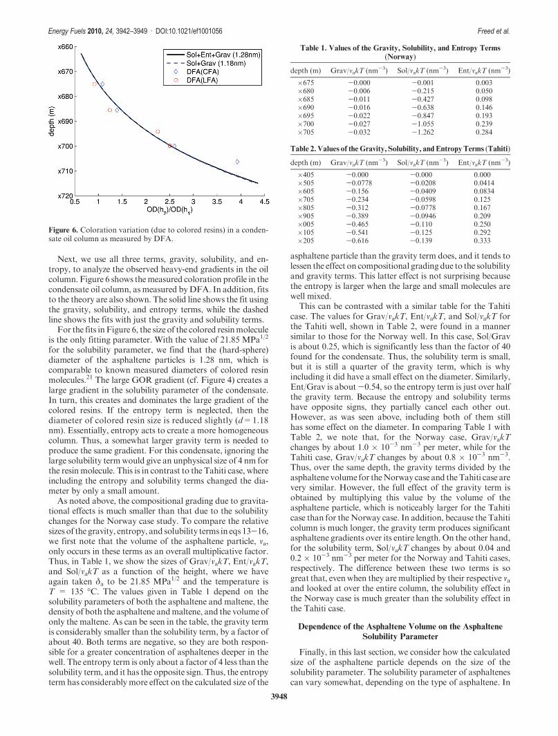
As noted above, the compositional grading due to gravita-tional effects is much smaller than that due to the solubilitychanges for the Norway case study. To compare the relativesizes of the gravity, entropy, and solubility terms in eqs 13-16,we first note that the volume of the asphaltene particle, va,only occurs in these terms as an overall multiplicative factor.Thus, in Table 1, we show the sizes of Grav/vakT, Ent/vakT,and Sol/vakT as a function of the height, where we haveagain taken δa to be 21.85 MPa1/2 and the temperature isT = 135 �C. The values given in Table 1 depend on thesolubility parameters of both the asphaltene and maltene, thedensity of both the asphaltene andmaltene, and the volume ofonly the maltene. As can be seen in the table, the gravity termis considerably smaller than the solubility term, by a factor ofabout 40. Both terms are negative, so they are both respon-sible for a greater concentration of asphaltenes deeper in thewell. The entropy term is only about a factor of 4 less than thesolubility term, and it has the opposite sign. Thus, the entropyterm has considerably more effect on the calculated size of the

asphaltene particle than the gravity term does, and it tends tolessen the effect on compositional grading due to the solubilityand gravity terms. This latter effect is not surprising becausethe entropy is larger when the large and small molecules arewell mixed.

This can be contrasted with a similar table for the Tahiticase. The values for Grav/vakT, Ent/vakT, and Sol/vakT forthe Tahiti well, shown in Table 2, were found in a mannersimilar to those for the Norway well. In this case, Sol/Gravis about 0.25, which is significantly less than the factor of 40found for the condensate. Thus, the solubility term is small,but it is still a quarter of the gravity term, which is whyincluding it did have a small effect on the diameter. Similarly,Ent/Grav is about-0.54, so the entropy term is just over halfthe gravity term. Because the entropy and solubility termshave opposite signs, they partially cancel each other out.However, as was seen above, including both of them stillhas some effect on the diameter. In comparing Table 1 withTable 2, we note that, for the Norway case, Grav/vakTchanges by about 1.0 � 10-3 nm-3 per meter, while for theTahiti case, Grav/vakT changes by about 0.8 � 10-3 nm-3.Thus, over the same depth, the gravity terms divided by theasphaltene volume for theNorway case and theTahiti case arevery similar. However, the full effect of the gravity term isobtained by multiplying this value by the volume of theasphaltene particle, which is noticeably larger for the Tahiticase than for the Norway case. In addition, because the Tahiticolumn is much longer, the gravity term produces significantasphaltene gradients over its entire length. On the other hand,for the solubility term, Sol/vakT changes by about 0.04 and0.2 � 10-3 nm-3 per meter for the Norway and Tahiti cases,respectively. The difference between these two terms is sogreat that, evenwhen they are multiplied by their respective vaand looked at over the entire column, the solubility effect inthe Norway case is much greater than the solubility effect inthe Tahiti case.

Dependence of the Asphaltene Volume on the Asphaltene

Solubility Parameter

Finally, in this last section, we consider how the calculatedsize of the asphaltene particle depends on the size of thesolubility parameter. The solubility parameter of asphaltenescan vary somewhat, depending on the type of asphaltene. In

Table 1. Values of the Gravity, Solubility, and Entropy Terms

(Norway)

depth (m) Grav/vakT (nm-3) Sol/vakT (nm-3) Ent/vakT (nm-3)

�675 -0.000 -0.001 0.003�680 -0.006 -0.215 0.050�685 -0.011 -0.427 0.098�690 -0.016 -0.638 0.146�695 -0.022 -0.847 0.193�700 -0.027 -1.055 0.239�705 -0.032 -1.262 0.284

Figure 6. Coloration variation (due to colored resins) in a conden-sate oil column as measured by DFA.

Table 2. Values of theGravity, Solubility, andEntropyTerms (Tahiti)

depth (m) Grav/vakT (nm-3) Sol/vakT (nm-3) Ent/vakT (nm-3)

�405 -0.000 -0.000 0.000�505 -0.0778 -0.0208 0.0414�605 -0.156 -0.0409 0.0834�705 -0.234 -0.0598 0.125�805 -0.312 -0.0778 0.167�905 -0.389 -0.0946 0.209�005 -0.465 -0.110 0.250�105 -0.541 -0.125 0.292�205 -0.616 -0.139 0.333

3949


addition, it also varies with temperature. For example, in ref18, the slight decrease in the solubility parameter as thetemperature is increased was found to be described by

δaðTÞ ¼ δaðT0Þ ½1- 1:07� 10- 3ðT -T0Þ� ð19Þwhere T0 is the reference temperature for the asphaltenesolubility parameter. On the other hand, the effect of thepressure on the asphaltene solubility parameter is usuallyignored because the asphaltenes are incompressible.

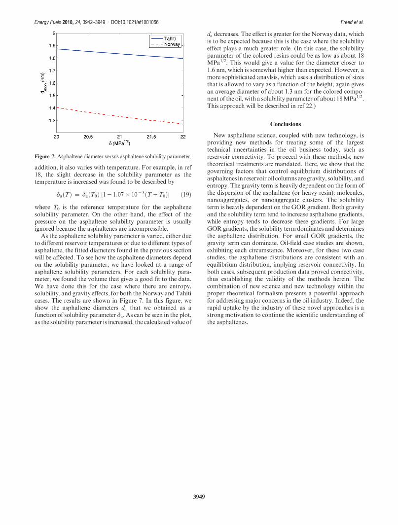
As the asphaltene solubility parameter is varied, either dueto different reservoir temperatures or due to different types ofasphaltene, the fitted diameters found in the previous sectionwill be affected. To see how the asphaltene diameters dependon the solubility parameter, we have looked at a range ofasphaltene solubility parameters. For each solubility para-meter, we found the volume that gives a good fit to the data.We have done this for the case where there are entropy,solubility, and gravity effects, for both theNorway and Tahiticases. The results are shown in Figure 7. In this figure, weshow the asphaltene diameters da that we obtained as afunction of solubility parameter δa. As can be seen in the plot,as the solubility parameter is increased, the calculated value of

da decreases. The effect is greater for the Norway data, whichis to be expected because this is the case where the solubilityeffect plays a much greater role. (In this case, the solubilityparameter of the colored resins could be as low as about 18MPa1/2. This would give a value for the diameter closer to1.6 nm, which is somewhat higher than expected. However, amore sophisticated anaylsis, which uses a distribution of sizesthat is allowed to vary as a function of the height, again givesan average diameter of about 1.3 nm for the colored compo-nent of the oil, with a solubility parameter of about 18MPa1/2.This approach will be described in ref 22.)

Conclusions

New asphaltene science, coupled with new technology, isproviding new methods for treating some of the largesttechnical uncertainties in the oil business today, such asreservoir connectivity. To proceed with these methods, newtheoretical treatments are mandated. Here, we show that thegoverning factors that control equilibrium distributions ofasphaltenes in reservoir oil columns are gravity, solubility, andentropy. The gravity term is heavily dependent on the form ofthe dispersion of the asphaltene (or heavy resin): molecules,nanoaggregates, or nanoaggregate clusters. The solubilityterm is heavily dependent on the GOR gradient. Both gravityand the solubility term tend to increase asphaltene gradients,while entropy tends to decrease these gradients. For largeGORgradients, the solubility term dominates and determinesthe asphaltene distribution. For small GOR gradients, thegravity term can dominate. Oil-field case studies are shown,exhibiting each circumstance. Moreover, for these two casestudies, the asphaltene distributions are consistent with anequilibrium distribution, implying reservoir connectivity. Inboth cases, subsequent production data proved connectivity,thus establishing the validity of the methods herein. Thecombination of new science and new technology within theproper theoretical formalism presents a powerful approachfor addressing major concerns in the oil industry. Indeed, therapid uptake by the industry of these novel approaches is astrong motivation to continue the scientific understanding ofthe asphaltenes.

Figure 7. Asphaltene diameter versus asphaltene solubility parameter.

theoretical treatment of asphaltene gradients in the presence of gor gradients

Documents