theoretical population biology - stanford university

Theoretical Population Biology 75 (2009) 331–345

Contents lists available at ScienceDirect

Theoretical Population Biology

journal homepage: www.elsevier.com/locate/tpb

An approximate likelihood for genetic data under a model with recombinationand population splittingD. Davisona,∗,1, J.K. Pritchardb,c, G. Coopb,2

a Committee on Evolutionary Biology, University of Chicago, United Statesb Department of Human Genetics, University of Chicago, United Statesc Howard Hughes Medical Institute, University of Chicago, United States

a r t i c l e i n f o

Article history:Received 26 January 2009Available online 9 April 2009

Keywords:Hidden Markov modelPAC likelihoodHaplotype dataPopulation history

a b s t r a c t

We describe a new approximate likelihood for population genetic data under a model in which a singleancestral population has split into two daughter populations. The approximate likelihood is based onthe ‘Product of Approximate Conditionals’ likelihood and ‘copying model’ of Li and Stephens [Li, N.,Stephens,M., 2003.Modeling linkage disequilibriumand identifying recombination hotspots using single-nucleotide polymorphism data. Genetics 165 (4), 2213–2233]. The approach developed here may be usedfor efficient approximate likelihood-based analyses of unlinked data. However our copying model alsoconsiders the effects of recombination. Hence, amore important application is to loosely-linked haplotypedata, for which efficient statistical models explicitly featuring non-equilibrium population structure haveso far been unavailable. Thus, in addition to the information in allele frequency differences about thetiming of the population split, the method can also extract information from the lengths of haplotypesshared between the populations. There are a number of challenges posed by extracting such information,which makes parameter estimation difficult. We discuss how the approach could be extended to identifyhaplotypes introduced by migrants.

© 2009 Elsevier Inc. All rights reserved.

1. Introduction

Population structure is a common feature of natural genetic andphenotypic variation (Mayr, 1942). For some applications, sum-marizing this structure by identifying subgroups and quantify-ing the extent of differentiation between them may be sufficient(e.g. Pritchard et al., 2000). However, the aim is often tomakemoreexplicit statements about the evolutionary history of the popula-tions. While some structured populations may be modeled as asystem of populations at equilibrium with respect to gene flow,researchers are often interested in non-equilibrium situations. Inparticular, at the interface of population genetics and phylogenywe are faced with the challenge of modeling population splitting.Accurate estimates of parameters such as the sizes of the popu-lations, the times at which they separated, and how much sub-sequent interbreeding there has been would be very valuable. Ifmechanisms limiting interbreeding between the populations have

∗ Corresponding author.E-mail address: [email protected] (D. Davison).

1 Current address: Department of Statistics, University of Oxford, UnitedKingdom.2 Current address: Department of Evolution and Ecology, and Center for

Population Biology, University of California, Davis, United States.

arisen, then fitting these models may allow us to decide whetherthis has occurred in parapatry or allopatry (Hey, 2006; Becquetand Przeworski, 2009). Furthermore, the identification of func-tional loci (such as those involved in reproductive isolation orlocal adaptation) will be facilitated by knowledge of populationhistory, effective population size and gene flow elsewhere in thegenome (Hey and Nielsen, 2004; Becquet and Przeworski, 2009).

Although there is awell-developed theory of population geneticprocesses that generate data under these types of scenarios (seee.g.Wakeley, 2008), it is often very difficult to compute likelihoodsfor models of interest. Therefore, in this paper we describe apromising alternative approach that approximates the standardlikelihood function. We start by specifying a particular model ofpopulation structure, and describing some of the approaches thathave been developed for this type of problem.

We focus on the most basic model of population splitting (seefor example Wakeley and Hey, 1997), in which an ancestralpopulation splits instantaneously into two daughter populations(see Fig. 1). The parameters of the model are the three effectivepopulation sizes (Na in the ancestral population; N1 and N2in the two daughter populations), the number of generationssince the splitting event (G), and the per-generation per-basepair probabilities of mutation and recombination (µ and r)respectively. Since our aim in this paper is to explore the utilityof a new approximate likelihood, we focus on a simple version

0040-5809/$ – see front matter© 2009 Elsevier Inc. All rights reserved.doi:10.1016/j.tpb.2009.04.001

http://dx.doi.org/10.1016/j.tpb.2009.04.001

http://www.elsevier.com/locate/tpb

http://www.elsevier.com/locate/tpb

mailto:[email protected]

332 D. Davison et al. / Theoretical Population Biology 75 (2009) 331–345

Fig. 1. Our model of population splitting without gene flow. Here, Na , N1 and N2indicate the effective population sizes in the ancestral population, and in the twodaughter populations, respectively. G is the number of generations since the split ofpopulations 1 and 2. The parameters F1 and F2 represent the amount of drift in thetwo daughter populations since the split.

of the model in which all three population sizes are equal(Na = N1 = N2 = N). The model with unequal population sizes isa straightforward generalization, described briefly in Section 3.2.As is typically the case in population genetics, the data in factcontain information about the parameters (G, µ, r) on the time-scale on which genetic drift occurs, rather than on a time-scale ofgenerations (see e.g. Wakeley, 2008). Thus our model in fact usesthe relative rate parameters θ = 2Nµ and ρ = 2Nr , and theparameter F = G/2N which represents the amount of drift that hasoccurred in the daughter populations since the split. Note that, as inmany coalescent-based models of population genetics, our modelof N diploids is equivalent to a model of 2N haploids (Wakeley,2008). Also note that θ and ρ are often defined to be twice thevalues that we use in this paper.

1.1. Types of data

Historically, non-recombining loci such as mitochondrial DNAhave often been used to fit these models, but there is a growingawareness of the statistical and biological limitations of suchdata sets (e.g. Hey and Machado, 2003). Therefore much researchnow focuses on using data from multiple unlinked regions of thegenome, which reflect multiple realizations of the genealogicalprocess. Often researchers will type a set of completely unlinkedmarkers (e.g. microsatellites or SNPs) scattered around thegenome, in which case the data can be summarized without loss ofinformation by the counts of the different alleles in eachpopulationat each locus. The expectations of various quantities can be derivedunder a model without migration (Wakeley and Hey, 1997), andthe likelihood of a particular configuration of allele counts at alocus may be computed analytically for a model with no migrationand where mutation since divergence can be ignored (e.g. Nielsenand Slatkin, 2000; Nicholson et al., 2002; Roychoudhury et al.,2008), or alternatively can be estimated accurately under moregeneral models using coalescent simulations.

While useful, completely unlinked loci offer only incompleteinformation about the genealogical process. One consequenceis that there is relatively low power to distinguish betweenisolation models with and without migration (Nielsen and Slatkin,2000), although multiallelic markers, such as microsatellites,hold additional information. With linked markers, the data arepotentially informative about both migration and splitting times,as one can hope to learn about the variability (i.e. the distribution),over loci, of the pairwise coalescence times between the twopopulations (Wakeley, 1996). The distribution is informative,

because under a model with no gene flow, the coalescence timesbetween different populations necessarily predate the time atwhich the population split; in contrast, if there has been somelow rate of gene flow, the coalescence times between populationsare more variable, as some lineages migrate and thus coalescemore recently (Wakeley, 1996). However, unlinked sites providelittle more information than the expectation of these times.For loosely linked data, information about the timing of thepopulation split and subsequent migration is captured by thelengths and similarities of haplotypes shared between populations,as ancestrally shared or migrant haplotypes are broken up byrecombination and diverge by mutation over time (e.g. Pooland Nielsen, 2008). For example, if two individuals in differentpopulations are found to be identical across a large chromosomalregion, then thismay be strong evidence for recent gene flow, sincesuch data may be unlikely under a pure split model.

1.2. Methods for linked data

Therefore, attention has turned to developing methods thatconsider a collection of genomic regions with linkage within eachregion, and free recombination between regions. Such data containinformation about the joint distribution of times in the genealogiesunderlying the data, and thus potentially contain much moreinformation about the parameters of interest. However, statisticalinference in this setting is difficult: the likelihoods cannot becomputed analytically and are difficult to estimate by simulationsince the observed data will be very improbable, or impossible,on the vast majority of genealogies simulated from the coalescentprior (see e.g. Stephens, 2001). This problem has given rise toa large literature on full-, summary- and approximate-likelihoodmethods for linked data, a very brief overview of which nowfollows.

Nielsen andWakeley (2001) and Hey and Nielsen (2004) devel-oped a full likelihood inference scheme for the isolation and mi-gration model, implemented by the IM software which can handlea set of independent fully linked loci. However, these approachesare limited, as extending them to allow intralocus recombinationis challenging even under simple demographic models (Fearnheadand Donnelly, 2001; Nielsen, 2000). This requirement of full link-age is a potentially serious drawback. Firstly, low-recombiningchromosomal regions may be atypical (Hilton et al., 1994); sec-ondly, authors frequently trim the regions used in order to fit theno-recombination requirement, which may result in bias (Hey andNielsen, 2004); and finally, this requirement limits the size of con-tiguous region that can be analyzed and hence the informationavailable.

Summary likelihood methods are based on replacing the datawith low-dimensional summary statistics, which allow likelihoodsand posterior densities to be estimated, typically by simulation(Pritchard et al., 1999; Beaumont et al., 2002; Cornuet et al.,2008). This approach has been extended to models of populationsplitting both with gene flow (Becquet and Przeworski, 2007)and without (Leman et al., 2005; Putnam et al., 2007). Intralocusrecombination can be incorporated straightforwardly, simply byallowing recombination in the simulated genealogies (e.g. Becquetand Przeworski, 2007). However, the flexibility and relative ease ofcomputation come at the expense of losing information, and noneof the existing approaches use summaries of the data that capturedetailed information about haplotype structure.

A promising recent development in population genetics infer-ence is the use of approximate likelihood approaches. One such ap-proach was developed by Li and Stephens (2003, henceforth, ‘‘LS’’)for inferring recombination rates. They developed a newmodel forpopulation genetic data that is simpler–andmore computationally

D. Davison et al. / Theoretical Population Biology 75 (2009) 331–345 333

tractable–than standardmodels. An attractive feature of the LS for-mulation is that it contains a formal model of haplotype structure,described in detail below.

The LS approach has been applied to inference in a diverse setof problems including estimating the parameters of recombination(Li and Stephens, 2003), mutation (Cornuet and Beaumont, 2007;Roychoudhury and Stephens, 2007), gene conversion (Gay et al.,2007; Yin et al., 2009) and diversifying selection (Wilson andMcvean, 2006). It has also been used as a tool for modelinghaplotype structure – rather than for formal parameter estimation– in genotype imputation and associationmapping (Marchini et al.,2007), HLA typing (Leslie et al., 2008) and in models of populationadmixture (Price et al., 2009) and clustering (Hellenthal et al.,2008).

In this study, we extend the LS approach to estimate theparameters of amodel of population splitting.While LS approachesare computationally convenient, they rely on ad hoc simplificationsof standard population genetic models, such as the coalescent.As such, a key challenge in extending the approach is to developapproximations that are suitable for the new problem. Ourapproach to this will be a central focus of the paper.

1.2.1. The original Li & Stephens modelThere are two main innovations in the LS approach. The first is

that it computes a likelihood for the full data by breaking it downinto a ‘product of approximate conditional’ (PAC) probabilities.Consider an observed set of haplotypes, H = h1, . . . , hn. The basicinference problem is to compute (and maximize) the likelihoodof the haplotype data H , with respect to the parameters φ ofa population genetic model. The likelihood can be written as aproduct of conditional probabilities:

L(H; φ) = pφ(h1)pφ(h2|h1) . . . pφ(hn|h1, . . . , hn−1). (1)

However, these conditional probabilities are unknown for mostmodels of interest, and the framework proposed by LS is basedinstead on the PAC likelihood

Lpac(H; φ) = pφ(h2|h1) . . . pφ(hn|h1, . . . , hn−1). (2)

Here, terms of the form pφ(hk+1|h1, . . . , hk) denote the (approx-imate) conditional probability of the (k + 1)th haplotype, condi-tional on the first k haplotypes, as a function of φ. We will refer tothese as ‘AC probabilities’. Note that under neutrality the uncon-ditional likelihood of the first haplotype does not usually dependstrongly on the model of population history. Therefore, followingLS, we set pφ(h1) = 1, and omit this term from our notation.

The second innovation of LS was to introduce a simple modelfor population genetic data under which these AC probabilitiesmay be computed. We will refer to this as their ‘‘copyingmodel’’. The model is an approximation which captures manyaspects of the coalescent with recombination, without sufferingfrom the computational difficulties that have hindered attemptsto incorporate recombination into coalescent-based MCMC andimportance sampling schemes. At a basic level, LS can be thoughtof as providing a simple model for simulating haplotype data. Wewill first briefly describe LS in terms of the simulation problem, andthen turn to how the LS model can be used for inference.

Consider first the simple case of data at a single SNP. Given kallele copies simulated so far, a new one is simulated by choosingone of the k uniformly at random: the newallele is said to ‘copy’ thechosen allele and, unless a mutation occurs, it is assigned the sameallelic state as the copied allele. (The genotype of the first alleleis set arbitrarily; e.g., to carry allele 0.) LS set the probability ofmutation to be a decreasing function of k, to reflect the expectationthat alleles added later in the order tend to match those alreadysampled (see Li and Stephens, 2003, for details).

Now consider simulating haplotypes at a set of loosely linkedsites. Let Xl be the label of the haplotype copied at site l by the newhaplotype. LS extended their model to include recombination byintroducing correlation between the Xs at nearby sites: unless a‘switch’ occurs, Xl+1 is the same as Xl. If there is a switch, then thehaplotype that is copied at the next site is a draw from the uniformprior on the k previously-sampled haplotypes (including the onethat was being copied at site l). Thus the new haplotype ismodeledas amosaic formed of stretches copied from the haplotypes alreadysimulated. Specifically, the probability distribution of the randomvariables denoting who is copied at each site (X1, X2, . . . , XL) is aMarkov chain along the sites. The switch events were intended tomimic the effects of recombination, and the transition probabilitiesof this Markov chain are controlled by a recombination parameterρ. As for mutation, the switch probability is also a decreasingfunction of k. This reflects the fact that a haplotype added into alarge sample tends to be similar to at least one other haplotypeover a large genetic distance.Computing the likelihood. There is a large set of possible valuesof the sequence X1, . . . , XL, i.e. which haplotype is copied by thenew haplotype at every site along the sequence, which we willrefer to as ‘paths’ through the missing data. To compute the ACprobability of the new haplotype pφ(hk+1|h1, . . . , hk) under thiscopying model, the paths are treated as missing data. Thus theAC probability is computed by averaging the data probability overthe prior probability distribution on the paths. The Markov chainpriormeans that this can be done efficiently using standard hiddenMarkov model (HMM) methods (e.g. Rabiner, 1989). It is thenstraightforward to calculate the PAC likelihood from these ACprobabilities according to Eq. (2).

One drawback of the scheme is that the use of approximateprobabilities in Eq. (2) means that the likelihood depends on theorder in which the haplotypes are added to the sample. LS found itsatisfactory for inference to sum over a small set of random orders,keeping the set of orders the same over the parameter values thelikelihood was estimated for.

1.3. Coalescing and copying

Full likelihood approaches for linked data, such as thatimplemented in the IM software (Hey and Nielsen, 2004, 2007),typically involve explicitly modeling aspects of the ancestralhistory of the sample such as the genealogical topology, thebranch lengths, details of movements of ancestral lineages, or thetypes of ancestral haplotypes (see e.g. Stephens, 2001). The PAClikelihood and copying model of LS may be seen as an ad hocapproximation of such a full likelihood scheme. From this pointof view, when modeling the new haplotype, its descent from theancestral lineages of the existing sample is mimicked by formingit as a mosaic of chunks copied from present-day haplotypeswith occasional ‘mutations’, and the uncertainty regarding itsrelationshipswith ancestral lineages of the existing sample is dealtwith by averaging over all possible copying paths.

Throughout this paper we make this link between the copyingprocess and the coalescent fairly explicit. That is, we considercopying haplotype X to be analogous to coalescing with theancestral lineage of haplotype X at some time in the past.With this analogy in mind, we construct our copying modelby deriving approximate probabilities and expectations under acoalescent model. This interpretation also lies behind the workof LS, who modeled the probabilities of mutation and switching(i.e. recombining) as decreasing functions of k, reflecting thefact that haplotypes added into an already large sample coalescerapidly with other haplotypes, leaving little time for mutation orrecombination (see Ewens (1990) for a discussion of this sequentialsampling construction of the coalescent process).


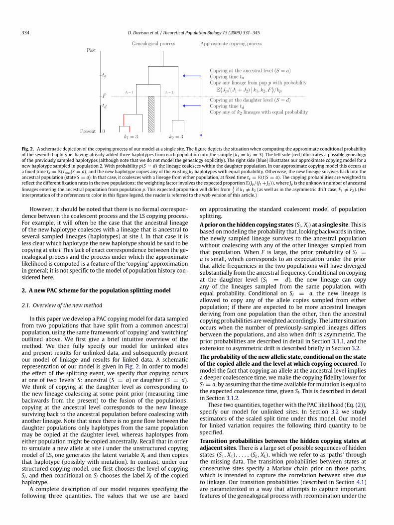
Fig. 2. A schematic depiction of the copying process of our model at a single site. The figure depicts the situation when computing the approximate conditional probabilityof the seventh haplotype, having already added three haplotypes from each population into the sample (k1 = k2 = 3). The left side (red) illustrates a possible genealogyof the previously sampled haplotypes (although note that we do not model the genealogy explicitly). The right side (blue) illustrates our approximate copying model for anew haplotype sampled in population 2. With probability p(S = d) the lineage coalesces within the daughter population. In our approximate copying model this occurs ata fixed time td = E(Tcoal|S = d), and the new haplotype copies any of the existing k2 haplotypes with equal probability. Otherwise, the new lineage survives back into theancestral population (state S = a). In that case, it coalesces with a lineage from either population, at fixed time ta = E(t|S = a). The copying probabilities are weighted toreflect the different fixation rates in the two populations; the weighting factor involves the expected proportion E(Jp/(J1 + J2)), where Jp is the unknown number of ancestrallineages entering the ancestral population from population p. This expected proportion will differ from 1

2 if k1 #= k2 (as well as in the asymmetric drift case, F1 #= F2). (Forinterpretation of the references to color in this figure legend, the reader is referred to the web version of this article.)

However, it should be noted that there is no formal correspon-dence between the coalescent process and the LS copying process.For example, it will often be the case that the ancestral lineageof the new haplotype coalesces with a lineage that is ancestral toseveral sampled lineages (haplotypes) at site l. In that case it isless clear which haplotype the new haplotype should be said to becopying at site l. This lack of exact correspondence between the ge-nealogical process and the process under which the approximatelikelihood is computed is a feature of the ‘copying’ approximationin general; it is not specific to themodel of population history con-sidered here.

2. A new PAC scheme for the population splitting model

2.1. Overview of the new method

In this paper we develop a PAC copyingmodel for data sampledfrom two populations that have split from a common ancestralpopulation, using the same framework of ‘copying’ and ‘switching’outlined above. We first give a brief intuitive overview of themethod. We then fully specify our model for unlinked sitesand present results for unlinked data, and subsequently presentour model of linkage and results for linked data. A schematicrepresentation of our model is given in Fig. 2. In order to modelthe effect of the splitting event, we specify that copying occursat one of two ‘levels’ S: ancestral (S = a) or daughter (S = d).We think of copying at the daughter level as corresponding tothe new lineage coalescing at some point prior (measuring timebackwards from the present) to the fusion of the populations;copying at the ancestral level corresponds to the new lineagesurviving back to the ancestral population before coalescing withanother lineage. Note that since there is no gene flow between thedaughter populations only haplotypes from the same populationmay be copied at the daughter level, whereas haplotypes fromeither population might be copied ancestrally. Recall that in orderto simulate a new allele at site l under the unstructured copyingmodel of LS, one generates the latent variable Xl and then copiesthat haplotype (possibly with mutation). In contrast, under ourstructured copying model, one first chooses the level of copyingSl, and then conditional on Sl chooses the label Xl of the copiedhaplotype.

A complete description of our model requires specifying thefollowing three quantities. The values that we use are based

on approximating the standard coalescent model of populationsplitting.Aprior on thehidden copying states (Sl, Xl) at a single site. This isbased onmodeling the probability that, looking backwards in time,the newly sampled lineage survives to the ancestral populationwithout coalescing with any of the other lineages sampled fromthat population. When F is large, the prior probability of Sl =a is small, which corresponds to an expectation under the priorthat allele frequencies in the two populations will have divergedsubstantially from the ancestral frequency. Conditional on copyingat the daughter level (Sl = d), the new lineage can copyany of the lineages sampled from the same population, withequal probability. Conditional on Sl = a, the new lineage isallowed to copy any of the allele copies sampled from eitherpopulation; if there are expected to be more ancestral lineagesderiving from one population than the other, then the ancestralcopying probabilities areweighted accordingly. The latter situationoccurs when the number of previously-sampled lineages differsbetween the populations, and also when drift is asymmetric. Theprior probabilities are described in detail in Section 3.1.1, and theextension to asymmetric drift is described briefly in Section 3.2.The probability of the new allelic state, conditional on the stateof the copied allele and the level at which copying occurred. Tomodel the fact that copying an allele at the ancestral level impliesa deeper coalescence time, we make the copying fidelity lower forSl = a, by assuming that the time available for mutation is equal tothe expected coalescence time, given Sl. This is described in detailin Section 3.1.2.

These two quantities, togetherwith the PAC likelihood (Eq. (2)),specify our model for unlinked sites. In Section 3.2 we studyestimators of the scaled split time under this model. Our modelfor linked variation requires the following third quantity to bespecified.Transition probabilities between the hidden copying states atadjacent sites. There is a large set of possible sequences of hiddenstates (S1, X1), . . . , (SL, XL), which we refer to as ‘paths’ throughthe missing data. The transition probabilities between states atconsecutive sites specify a Markov chain prior on those paths,which is intended to capture the correlation between sites dueto linkage. Our transition probabilities (described in Section 4.1)are parameterized in a way that attempts to capture importantfeatures of the genealogical process with recombination under the


Fig. 3. The copying process in the new PACmodel for loosely linked data illustratedwith an example path through the missing data. A new haplotype is added to asample of four (k1 = 2, k2 = 2; population labels are given on the right handside). At each site along the haplotypes, small circles represent which of the twoalleles is present (filled or open). Each of the 4 haplotypes has its own color. Thenew haplotype at the bottom is made up as a mosaic of these colors, indicatingwhich of the four haplotypes is copied at each site (X1, X2, . . . , XL), and letters (dand a) indicate which level this copying occurs at (S1, S2, . . . , SL). For each of the5 copied sections, a schematic genealogy is drawn above that might correspond tothe state of the copying process below. In the trees, the new lineage is depicted inblack. Although the relationships of the colored lines in the genealogies are depictedas remaining the same, note that this is not an assumption of the model.

population splitting model. Thus the new haplotype is modeledas a mosaic of sections of haplotype copied from one of theprevious haplotypes, where points at which there is a switch in thehaplotype being copied correspond to recombination events.

When F is large we have already seen that the prior at asingle site places relatively little weight on ancestral copying.Our transition probabilities have the effect that these occasionalstretches of ancestral copying are short, since the deep split timegives plenty of time for recombination. Therefore, the haplotypeis expected to resemble others from the same population overlong stretches. Conversely, when there has been less drift sincethe split, higher prior probability is associated with copying longersections of ancestral haplotypes. We capture these properties ofthe genealogical process with recombination by using expectedcoalescence times in the daughter and ancestral populationsto model the opportunity for recombination (switching) in ourapproximate copying process.

Fig. 3 illustrates a possible sequence of hidden states. Thevalues of X along the haplotype are indicated by the haplotypecoloring, and the values of S are indicated by the sequence of lettersunderneath. The path that is illustrated is one that might havehigh prior probability when F is relatively large because, firstly,the sections that are copied at the daughter level are much longerthan those copied ancestrally, and secondly, the ancestral-levelcopying hasmademore errors (mutations) than the daughter-levelcopying.Computing the likelihood. To compute the AC probability we haveto consider the set of all possible paths (S1, X1), . . . , (SL, XL). Theprior probability of one of these paths will depend on the value ofthe parameters F and ρ, as well as on the numbers k1 and k2 ofhaplotypes added so far from each population. The AC probability,pφ(hk1+k2+1|h1, . . . , hk1+k2), corresponds to the probability of thedata averaged over this prior probability distribution on possiblepaths and, as in LS, can be computed in an efficient manner usingthe forward algorithm for hidden Markov models (HMMs; see e.g.Rabiner (1989) and Appendix A).

As in LS, the approximations made in our PAC model makethe likelihood depend upon the ordering of the haplotypes, and

we average the likelihood of a dataset over a small set of randomorders of haplotypes. For the results presented here we constrainthese random orders to sample a haplotype from each of the twopopulations in turn.

3. Unlinked data

3.1. Methods: Unlinked

In the unlinked case the likelihood for the alignment ofhaplotypes may be computed as the product of the likelihoods forindividual sites. Therefore, in this section we will use hi to referto an allele copy at a single site rather than an entire haplotype.The problem of computing the likelihood is now reduced tocomputing the approximate probability of a new allele hk1+k2+1given the alleles h1, . . . , hk1+k2 observed so far, as a function of themodel parameters. To do so we now specify our prior probabilitydistribution on the hidden copying states Sl ∈ {a, d} and Xl ∈{1, . . . , k1 + k2}, as well as the mutation probability conditionalon the level at which copying occurs.

3.1.1. The prior on Sl and XlIn contrast to LS, under our population splittingmodel the prior

probability on Xl is uniform only in the unstructured case F = 0. Tomodel the structure we introduce an additional state Sl, the priorprobability distribution of which is given by the probability p(Sl =a) that the new lineage coalesces in the ancestral population, giventhe amount of drift in the population from which it was sampled,and the number of lineages already sampled from that population.The probability is a decreasing function of both the latter twoquantities, capturing the idea that few lineages make it back tothe ancestral population in populations that have experiencedconsiderable drift, and that lineages added later in the orderare a priori more likely to coalesce in the daughter populationand so resemble alleles already sampled within that population.The probability can be calculated exactly for a coalescent model(Eq. (31), Appendix C.1).

Conditional on Sl, we use the following prior probabilitydistribution on Xl:

p(Xl = i|Sl = d) =

1kz∗

if zi = z∗

0 otherwise(3)

p(Xl = i|Sl = a) = E(

JziJ1 + J2

)1kzi

. (4)

Here, zi ∈ {1, 2} is the population label of sampled lineage i,and kzi refers to the number of lineages sampled so far frompopulation zi. z∗ is shorthand notation for zk1+k2+1, i.e. the labelof the population from which the new lineage is sampled. Jzi is theunknownnumber of distinct ancestral lines that enter the ancestralpopulation, starting with kzi lines in daughter population zi. Theexpectation can be calculated using the transition probabilities inTavaré (1984) (Appendix C Eq. (32)). Note that although quantitiessuch as p(Sl = a) and p(Xl = i|S) depend on k1, k2, and F , thisdependence is generally left implicit in our notation.

In words, conditional on copying in the daughter population,the prior on ‘who you copy’ has zero weight on alleles fromthe other population, and is uniform over alleles from the samepopulation. The prior, conditional on copying ancestrally, allowsany allele to be copied but takes into account the numbers ofallele copies sampled so far from each population (k1 and k2). Thisprior extends straightforwardly to the case of unequal drift in thedaughter populations, as discussed in Section 3.2.


3.1.2. Mutation probabilityConditional on copying in the daughter population, the

probability that the new allele is identical to the copied alleleshould be (as in LS) an increasing function of kz∗ , since when kz∗is large we expect the new lineage to coalesce rapidly into theexisting tree. Furthermore, since Sl = a implies a more ancientcoalescence time than Sl = d whatever the value of k1 and k2, theancestral copying fidelity is lower. The approachwe take is to viewthe mutation probability in terms of the opportunity for mutationbefore the copying (coalescence) time ts. We set this time to itsexpectationts = E(Tcoal|S = s; k1, k2, F), (5)where Tcoal is the coalescence time of the (k1 + k2 + 1)th lineage.

These expectations can be computed exactly using results fromTavaré (1984) and Fu and Li (1993) (see Appendix C). Themutationprobabilities used are based on the assumption that either 0 or1 mutations occurred on the branch joining the new line to theexisting tree and areu(hk1+k2+1|hi, s) = p(hk1+k2+1|Sl = s, Xl = i; k1, k2, F)

={1 − exp(−θ ts) if hk1+k2+1 #= hi

exp(−θ ts) if hk1+k2+1 = hi.(6)

An exception occurswhen k = 1 inwhich case 2ta is substitutedfor ta in order to account for the time on the branch ancestral tothe first line (S = d is impossible for the second line sampled, asthe randomorderings are chosen such that haplotypes are sampledalternately from each population).

The value of θ depends on the way in which the sampledloci were ascertained. If the loci were selected without regardto whether or not they show polymorphism (resequencing data),then θ would be treated as a parameter of the model to beestimated. Alternatively, if loci were only included if they werepolymorphic in the sample (SNP data) then, following LS, anarbitrary small value of θ is used. For the results presented inthis paper we used θ = 1/E(Ttotal), where Ttotal is the expectedtotal length of the full genealogy with n tips, given the sampleconfiguration and the model parameters. This can be calculatedexactly (Wakeley and Hey, 1997) but in the implementationdescribed here we used an approximation (Appendix C.3).

3.1.3. Calculating the likelihood of unlinked dataThe AC probability under the isolation model is obtained by

averaging the mutation probability over the prior probabilitydistribution on the missing data:

pφ(hk1+k2+1|h1, . . . , hk1+k2) =∑

s∈{d,a}

k1+k2∑

i=1

u(hk1+k2+1|hi, s)

× p(S = s, X = i).

Let u(hk1+k2+1|s) = ∑k1+k2i=1 u(hk1+k2+1|hi, s)p(X = i|S = s)

denote the emission probability averaged over which allele iscopied, given that S = s. Then the AC probability under isolationwithout gene flow ispφ(hk1+k2+1|h1, . . . , hk1+k2) = p(S = a)u(hk1+k2+1|S = a)

+ (1 − p(S = a))u(hk1+k2+1|S = d). (7)Eqs. (2), (6) and (7), together with the expressions for p(S = a)

and ts given in Appendix C, specify an algorithm for computing thePAC likelihood under the isolation without gene flow model, for asingle ordering of alleles. The likelihoods that we actually use arean average of these quantities over a random sample of orderings,subject to taking alleles alternately from the two populations.For the results in this paper we have used 10 random orderings.We implemented the algorithms described in this paper in R (RDevelopment Core Team, 2008).

5

4

3

2

1

0

0

1 2 3 4 5 6 7 8 9 10

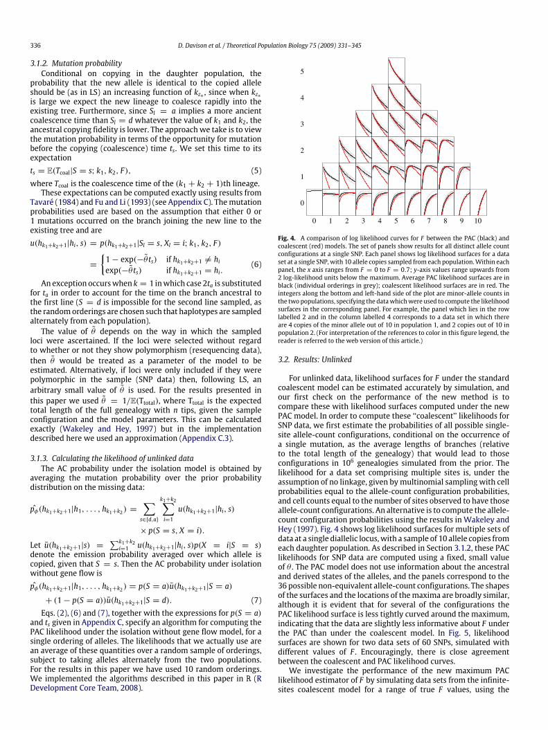
Fig. 4. A comparison of log likelihood curves for F between the PAC (black) andcoalescent (red) models. The set of panels show results for all distinct allele countconfigurations at a single SNP. Each panel shows log likelihood surfaces for a dataset at a single SNP, with 10 allele copies sampled from each population.Within eachpanel, the x axis ranges from F = 0 to F = 0.7; y-axis values range upwards from2 log-likelihood units below the maximum. Average PAC likelihood surfaces are inblack (individual orderings in grey); coalescent likelihood surfaces are in red. Theintegers along the bottom and left-hand side of the plot are minor-allele counts inthe two populations, specifying the datawhichwere used to compute the likelihoodsurfaces in the corresponding panel. For example, the panel which lies in the rowlabelled 2 and in the column labelled 4 corresponds to a data set in which thereare 4 copies of the minor allele out of 10 in population 1, and 2 copies out of 10 inpopulation 2. (For interpretation of the references to color in this figure legend, thereader is referred to the web version of this article.)

3.2. Results: Unlinked

For unlinked data, likelihood surfaces for F under the standardcoalescent model can be estimated accurately by simulation, andour first check on the performance of the new method is tocompare these with likelihood surfaces computed under the newPAC model. In order to compute these ‘‘coalescent’’ likelihoods forSNP data, we first estimate the probabilities of all possible single-site allele-count configurations, conditional on the occurrence ofa single mutation, as the average lengths of branches (relativeto the total length of the genealogy) that would lead to thoseconfigurations in 106 genealogies simulated from the prior. Thelikelihood for a data set comprising multiple sites is, under theassumption of no linkage, given bymultinomial sampling with cellprobabilities equal to the allele-count configuration probabilities,and cell counts equal to the number of sites observed to have thoseallele-count configurations. An alternative is to compute the allele-count configuration probabilities using the results in Wakeley andHey (1997). Fig. 4 shows log likelihood surfaces for multiple sets ofdata at a single diallelic locus,with a sample of 10 allele copies fromeach daughter population. As described in Section 3.1.2, these PAClikelihoods for SNP data are computed using a fixed, small valueof θ . The PAC model does not use information about the ancestraland derived states of the alleles, and the panels correspond to the36 possible non-equivalent allele-count configurations. The shapesof the surfaces and the locations of themaxima are broadly similar,although it is evident that for several of the configurations thePAC likelihood surface is less tightly curved around the maximum,indicating that the data are slightly less informative about F underthe PAC than under the coalescent model. In Fig. 5, likelihoodsurfaces are shown for two data sets of 60 SNPs, simulated withdifferent values of F . Encouragingly, there is close agreementbetween the coalescent and PAC likelihood curves.

We investigate the performance of the new maximum PAClikelihood estimator of F by simulating data sets from the infinite-sites coalescent model for a range of true F values, using the

D. Davison et al. / Theoretical Population Biology 75 (2009) 331–345 337–1

0–8

–6–4

–20

0.0 0.1 0.2 0.3 0.4 0.5 0.6 0.7 0.0 0.1 0.2 0.3 0.4 0.5 0.6 0.7

–10

–8–6

–4–2

0

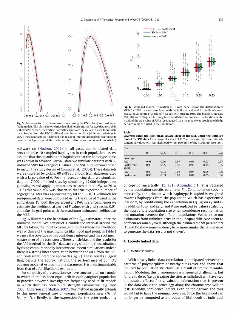
Fig. 5. Inference for F in the unlinked model using the PAC (black) and coalescent(red) models. The plots show relative log likelihood surfaces for two data sets of 60unlinked SNPs each. The vertical dotted lines indicate the value of F used to simulatedata. Results from the PAC likelihood are plotted in black (different orderings ingrey); the coalescent log likelihood is in red. (For interpretation of the references tocolor in this figure legend, the reader is referred to the web version of this article.)

software ms (Hudson, 2002). In all cases our simulated datasets comprise 10 sampled haplotypes in each population, i.e. weassume that the organisms are haploid or that the haplotype phasewas known in advance. For SNP data we simulate datasets with 60unlinked SNPs for a range of F values. (The SNP numberwas chosento match the study design of Conrad et al. (2006)). These data setswere simulated by picking 60 SNPs at random from data generatedwith a large value of θ . For the resequencing data we simulateddata at 17,000 unlinked sites by simulating 17,000 independentgenealogies and applying mutations to each at rate 4Nµ = 2θ =10−3 (this value of θ was chosen so that the expected number ofsegregating sites was approximately 60 at F = 0). Likelihoods forresequenced data were computed using the value of θ used in thesimulations. For both the coalescent and PAC inference schemesweestimate the likelihood at a grid of F values with grid-spacing 0.01,and take the grid point with the maximum estimated likelihood asthe MLE.

Fig. 6 illustrates the behaviour of the Fpac estimator under theunlinked model. We construct a confidence interval around theMLE by taking the most extreme grid points whose log likelihoodwas within 2 of the maximum log likelihood grid point. In Table 1we give the coverage of this confidence interval, and the rootmeansquare error of the estimators. There is little bias, and the results forthe PACmethod for the SNP data are very similar to those obtainedby using computationally intensive coalescent simulations. Indeedthere is a strong linear correlation between the MLE from the PACand coalescent inference approach (Fig. 7). These results suggestthat, despite the approximations, the performance of our PACcopying model at estimating the parameter F is indistinguishablefrom that of a full likelihood estimator.

For simplicity of presentationwe have concentrated on amodelin which there has been equal drift in each daughter population.In practice however, investigators frequently need to fit modelsin which drift has been quite strongly asymmetric (e.g. Hey,2005; Anderson and Slatkin, 2007). Our method naturally extendsto this more general case of unequal population sizes (N1 #=N2 #= Na). Briefly, in the expression for the prior probability

0.3

0.0

0.1

0.4

0.2

0.5

0.00 0.05 0.10 0.15 0.20 0.25

SNPs – coalescentSNPs – PACreseq – PAC

Fig. 6. Unlinked model: Estimation of F . Each panel shows the distribution ofMLEs for 1000 data sets simulated with the indicated value of F . Likelihoods wereevaluated at points of a grid of F values with spacing 0.01. The boxplots indicate25%, 50% and 75% quantiles. Long horizontal black bars indicate the location on they-axis of the true value of F . For resequenced data themodel was provided with theper-site value of θ used in the simulations.

Table 1Coverage rates and Root Mean Square Error of the MLE under the unlinkedmodel for SNP data for a range of values of F . The coverage rates use intervalscontaining values with log-likelihood within two units of the maximum (see text).

Ftrue0 0.05 0.1 0.15 0.2 0.25

CoveragePAC 0.98 0.96 0.97 0.96 0.97 0.97Coalescent 0.98 0.95 0.96 0.95 0.95 0.95RMSEPAC 0.01 0.03 0.04 0.04 0.05 0.06Coalescent 0.01 0.03 0.03 0.04 0.05 0.06

of copying ancestrally (Eq. (31), Appendix C.1), F is replacedby the population-specific parameter Fz∗ . Conditional on copyingancestrally, the prior on which haplotype is copied is weightedtowards haplotypes from the population which has experiencedless drift, by conditioning the expectation in Eq. (4) on F1 and F2in addition to k1 and k2. ρ and θ are replaced by values scaled bythe appropriate population size when considering recombinationandmutation events in the different populations.We note that ourestimators from unlinked SNPs in the unequal drift case seem toperform reasonably well, although the estimated drift parameters(F1 and F2) show some tendency to bemore similar than those usedto generate the data (results not shown).

4. Loosely linked data

4.1. Methods: Linked

With loosely linked data, correlation is anticipated between thepatterns of polymorphism at nearby sites (over and above thatinduced by population structure), as a result of limited recombi-nation. Modeling this phenomenon is in general challenging, butfailure to do so (i.e by treating the sites as unlinked) will have twoundesirable effects: firstly, valuable information that is presentin the data about the genealogy along the chromosome will belost; secondly, confidence intervals can be too narrow, and thuswould fail to have the nominal coverage. Since the likelihood canno longer be computed as a product of likelihoods at individual


0.0 0.1 0.2 0.3 0.4 0.5

0.0

0.2

0.4 F = 0

0.0 0.1 0.2 0.3 0.4 0.5

0.0

0.2

0.4 F = 0.05

0.0 0.1 0.2 0.3 0.4 0.5

0.0

0.2

0.4 F = 0.1

0.0 0.1 0.2 0.3 0.4 0.5

0.0

0.2

0.4 F = 0.15

0.0 0.1 0.2 0.3 0.4 0.5

0.0

0.2

0.4 F = 0.2

0.0 0.1 0.2 0.3 0.4 0.5

0.0

0.2

0.4 F = 0.25

Fig. 7. Unlinked model: Estimation of F . Each panel shows the joint distribution ofcoalescent (x-axis) and PAC (y-axis) MLEs for 1000 SNP data sets simulatedwith theindicated value of F . Darker colors indicate higher local density of points. Grey linesindicate the true value of F , and the line y = x. Red crosses lie at the mean valueof the MLEs. Likelihoods were evaluated at points of a grid of F values with spacing0.01. (For interpretation of the references to color in this figure legend, the readeris referred to the web version of this article.)

sites, we now switch notation so that hi refers to haplotype i, asopposed to a single allele copy as it did in the previous section.

Recall that our model involves, at each site l, the unknowncopying states Sl (the level at which copying occurs) and Xl (theidentity of the haplotype that is copied). Whereas the unlinkedcase simply required the specification of the prior distributionon (Sl, Xl) at a single site, in the linkage model the copyingstates at nearby sites are not independent under the prior. Henceit is less straightforward to specify the joint prior distributionon the copying states (S1, X1), . . . , (SL, XL) at all sites. As in LS,we use a Markov chain for this prior. Therefore, in additionto the marginal (single-site) prior on (Sl, Xl), we also specifytransition probabilities between (Sl, Xl) and (Sl+1, Xl+1). Thesegovern properties such as the expected length of stretches ofancestral copying, and must be appropriately parameterized bymodel parameters such as F , as well as by k1 and k2. The otherparameter that features in these transition probabilities is ρl,which corresponds to the population-scaled recombination ratebetween sites l and l + 1. We focus on the case of constantrecombination rate along the chromosome, so ρl corresponds tothe population-scaled, per base-pair rate of recombination (ρbp)multiplied by the physical distance between site l and l + 1.Variation in recombination rates along the chromosome could beincorporated simply by setting the ρl individually, according toan estimated genetic map. Since we view (Sl = s, Xl = i) as astatement about the way in which the new lineage coalesces into the existing genealogy at site l, in order to parameterize thetransition probabilities we consider how recombination can resultin changes to this genealogical structure.

The transition probabilities have the following form:p(Sl+1 = s′, Xl+1 = i′|Sl = s, Xl = i) = pR(Sl+1 = s′|Sl = s)

× p(Xl+1 = i′|Sl+1 = s′) + I(i′ = i, s′ = s)p(NR|Sl = s). (8)In this expression I() is an indicator function that takes the value1 if its argument is true and 0 otherwise, and p(NR|Sl = s) is

the probability, given that copying is at level s, that there is norecombination between sites l and l + 1, resulting in no changeof state (i′ = i, s′ = s). p(Xl+1 = i′|Sl+1 = s′) is the probabilityof copying haplotype i′ given copying at level s′, and is the sameas in the no-linkage model (Eqs. (3) and (4)). The tricky part hereis pR(Sl+1 = s′|Sl = s), which is the probability, given copying atlevel s at site l, that a recombination occurs between sites l andl+ 1 and that as a result copying occurs at level s′ at site l+ 1. Ourcopying process is an approximation to the coalescent model andso our aim is that, for example, pR(Sl+1 = a|Sl = d) approximatesthe probability, conditional on coalescence of the new lineage in itsown population at site l, that there is recombination between sitesl and l + 1 and the genealogy is altered in such a way that at sitel + 1 the same line now coalesces in the ancestral population.

We approximate the transition probabilities by consideringdifferent classes of genealogical rearrangements which could giverise to the copying transition in question, as illustrated in Fig. 8.That figure is divided into four panels, corresponding to the fourdifferent transitions (d → d, d → a, a → d and a → a). Withineach panel, the different classes of genealogical rearrangement areidentified by a number (i)–(v). We now explain the expressionsthat we use for the quantities p(NR|Sl = s) and pR(Sl+1 = s′|Sl = s)in more detail. When describing the genealogical motivation forthese expressions, we will refer to the ancestral lineage of thehaplotype that is copied at site l as the ‘‘copied lineage’’.

4.1.1. Transition probabilities under the linkage modelTransitions from the daughter population. We consider twopossibilities involving recombination: a recombination occurs oneither the new lineage or the copied lineage, prior to theircoalescence (event Rdc ; genealogies i and iii in the d → a and thed → d panels of Fig. 8). The coalescence time of these lineagesis assumed to be the conditional expectation td. Therefore for theprobability of no recombination—and thus no change in state—weuse

p(NR|Sl = d) = 1 − p(Rdc) (9)

where

p(Rdc) = 1 − exp(−2ρltd). (10)

If there is a recombination, the new lineage subsequently coalescesinto the tree at the next site either in the daughter (S ′ = d) orancestral (S ′ = a) population. Following from Eq. (9), in principlethe probability of the transition as a result of recombination shouldbe

pR(Sl+1 = s′|Sl = d) = p(Rdc)p(Sl+1 = s′|Rdc). (11)

However, evaluating e.g. p(Sl+1 = a|Rdc) requires averaging theprobability of surviving back to the ancestral population over theunknown number of uncoalesced lines at the unknown time of therecombination event; in practicewe substitute themarginal (prior)probability p(S = s′) (Eq. (31), Appendix C.1), which is larger thanp(S = s′|Rdc) in the case s′ = d and smaller in the case s′ = a.Transitions from the ancestral population. In the case of a → aand a → d we classify the recombination events according towhether they occur on the new lineage in the daughter population(event Rn

d), on the copied lineage in the daughter population (eventRod) (genealogies i and iii in Fig. 8) or on either line in the ancestral

population, before they coalesce (event Rac) (genealogies ii andiv). The length of time available for recombination in a daughterpopulation is F , and in the ancestral population we approximate itby ta−F . Thuswe approximate the probability of no recombination(genealogy v) by

p(NR|Sl = a) = (1 − p(Rnd ∪ Ro

d ∪ Rac)) (12)


Fig. 8. Transitions between daughter and ancestral copying states. The four panels correspond to the four possible transitions between copying levels (d → d, d → a,a → d and a → a). Within each panel, we illustrate the various classes of genealogical rearrangement that we consider when approximating the probability of that panel’scopying transition. Each class of genealogical rearrangement is illustrated by a diagram of a genealogy of two lineages (in black): the new lineage (marked with an asterisk),and the lineage that it copies at site l. In each genealogy diagram, a thick blue line represents the barrier to gene flow separating the daughter populations. At site l + 1, thelineage that is copied may be different as a result of recombination in the history of the two samples between sites l and l + 1. Red lines represent lineages at site l + 1, andthe way they are drawn reflects the way in which the probability of the event being depicted depends on their fate (i.e. on when they coalesce into the rest of the genealogy).Short red rising lines indicate that the transition probability depends only on the occurrence of the recombination event, and not otherwise on the fate of the recombinantline. Long red rising lines indicate that the lineage must remain distinct and enter the ancestral population, prior to its eventual recoalescence. A horizontal terminus to thered line indicates that the line must recoalesce in the daughter population. Red lines without an initial horizontal section do not require a recombination to have occurred(i.e. they already existed at site l). The five types of event are, (i) recombination on the new lineage in the daughter population, (ii) recombination on the new lineage inthe ancestral population, (iii) recombination on the copied lineage in the daughter population, (iv) recombination on the copied lineage in the ancestral population, (v) nointerrupting event (note that this last event can only contribute to the probability of ‘transitions’ to the same haplotype at the same level (s′ = s, i′ = i)). (For interpretationof the references to color in this figure legend, the reader is referred to the web version of this article.)

wherep(Rn

d ∪ Rod ∪ Rac) = 1 − exp(−2ρlta). (13)

The case a → d is relatively straightforward as only a recombi-nation event on the new lineage in the daughter population (ge-nealogy i), followed by recoalescence in the daughter population,can effect this transition. Thus the expression that we use for thea → d transition probability as a result of recombination ispR(Sl+1 = d|Sl = a) = p(Rn

d)p(S = d|Rnd), (14)

where p(Rnd) = 1 − exp(−ρlF). Again, we substitute the

unconditional prior probability p(S = d) for p(S = d|Rnd).

The case a → a is more complex, as this transition can resultfrom any of the following (mutually exclusive) combinations ofevents:• a recombination on the new lineage in the daughter population

(genealogy i), followed by ancestral recoalescence; probabilityp(Rn

d)p(S = a|Rnd);• no recombination on the new lineage in the daughter popula-

tion, but recombination on the copied lineage in the daughterpopulation, (genealogy iii); probability (1 − p(Rn

d))p(Rod)• recombination on neither the new or copied lineage in the

daughter population but an ancestral recombination on one orother lineage, (genealogies ii and iv); probability (1 − p(Rn

d ∪Rod))p(Rac).

Thus the expressionwe use for the a → a transition probabilityas a result of recombination ispR(Sl+1 = a|Sl = a) = p(Rn

d)p(S = a) + (1 − p(Rnd))p(R

od)

+ (1 − p(Rnd ∪ Ro

d))p(Rac) (15)wherep(Ro

d) = p(Rnd) = 1 − exp(−ρlF)

p(Rnd ∪ Ro

d) = 1 − exp(−2ρlF)

p(Rac) = 1 − exp(−2ρl(ta − F)), (16)and again we have substituted the marginal (prior) probabilityp(S = a) instead of p(S = a|Rn

d).

4.2. Results: Linked

We now explore the properties of our PAC scheme for looselylinked regions. Again, we focus on the symmetric case in which theamount of drift has been the same in the twodaughter populations,and in which the ancestral population had the same effective sizeas the daughter populations. In keeping with LS and much of thesubsequent development of PAC copying models (e.g. Yin et al.,2009; Marchini et al., 2007; Leslie et al., 2008; Price et al., 2009;Hellenthal et al., 2008), we focus here on estimation under themodel for SNP data rather than resequencing data (methodologicalaspects of fitting the linkage model to resequencing data arediscussed in Appendix B).

To illustrate how our method uses the information in linkage,and to provide a comparison with LS, we begin by investigatingthe ability of ourmethod to estimate the recombination parameterρ (where ρ is ρbp multiplied by the length of the genomicregion simulated). Fig. 9 illustrates the relationship between themaximum PAC likelihood estimator ρpac, and the true value of ρ.Since this relationship may vary with the value of F used in thesimulation, and when fitting the model, the figure displays resultsfor data simulated using four different values of F . In each case thetrue value of F was usedwhen fitting themodel.When the data aresimulatedwithout recombination, ρpac is generally close to zero. Ascan be seen in Fig. 9, our estimates of ρ are biased, but there is alinear relationship between ρ and ρpac, the slope of which variesbetween 0.25 at F = 0 and 0.45 at F = 0.2.

Whereas LS were primarily concerned with estimating therecombination rate, our focus here is on estimating the driftparameter F . The linkage model incorporates information aboutthe lengths of haplotypes shared within and between populationsinto the estimation of F , and therefore these estimates areinfluenced by the value of ρ used when fitting the model. Fig. 10illustrates the dependence of Fpac on F , for some different valuesof ρ. It is evident that if the value of ρ is increased, the modelresponds by lowering the estimate of F . A partial explanation of


F=0

y=4.8+0.24x

050

100

150

200

F=0.05

y=5.1+0.37x

F=0.1

y=4.5+0.42x

F=0.2

y=4.2+0.44x

050

100

150

200

0 50 100 150 200

0 50 100 150 200 0 50 100 150 200

0 50 100 150 200

050

100

150

200

050

100

150

200

Fig. 9. Dependence of ρpac on ρ. 60 SNPs were simulated using the specified valueof ρ for the region, for four different values of F . When fitting themodel to estimateρpac for each region, F was fixed at its true value. The line y = x is shown in lightgray. The results of a linear regression of ρpac on ρ are shown as a black line and anequation in each panel.

rho = 0.5 x true rhorho = 0.75 x true rhorho = 1 x true rho

0.0

0.1

0.2

0.3

0.4

0.5

0.6

0.00 0.05 0.10 0.15 0.20 0.25

Fig. 10. Linkage model: Estimation of F (symmetric drift, SNP data). The x-axisindicates the value of F used to simulate the data. For each value of F , 200 datasets of 60 SNPs were simulated with 4Nr = 2ρ = 50. Above each value of F ,distributions of Fpac MLEs are illustrated with boxplots. The 3 boxplots correspondto different values of ρ used when fitting themodel. The boxplots indicate 25%, 50%and 75% quantiles of the MLEs and the mean MLEs are indicated by a solid blackdots. Horizontal black bars indicate the location on the y-axis of the true value of F .

this phenomenon is provided by considering stretches of similaritybetween haplotypes from different populations. The distributionof lengths of such stretches under the prior is determined by theproduct ρF = rG. Therefore if ρ is increased, then the modelresponds by decreasing the estimate of F .

Although no value of ρ results in unbiased estimation of Facross the range of F valueswe investigated, it is possible to almost

no–linkage modelbias–corrected linkage model

0.0

0.2

0.4

0.6

0.00 0.05 0.10 0.15 0.20 0.25

Fig. 11. Bias correction under the linkage model. The figure shows the distributionof MLEs for 100 data sets simulated with the value of F indicated along the x-axis.The boxplots indicate 25%, 50% and 75% quantiles of the MLEs and the mean MLEsare indicated by solid black dots. Horizontal blue bars indicate the location on the y-axis of the true value of F . MLEs from the bias-corrected linkagemodel (see text) areshown in blue. MLEs resulting from analysing the same data under the no-linkagemodel are shown in red. (For interpretation of the references to color in this figurelegend, the reader is referred to the web version of this article.)

completely correct this bias. To do this we fit a linear model

Fpac ∼ a + bFtrue (17)

for the Fpac MLE estimates, using a fixed value of ρ across arange of simulations with different Ftrue. We then construct a newestimate with reduced bias by removing the linear componentof the bias (Fpac − a)/b. We did this for the values of ρ shownin Fig. 10, using 100 simulations for each Ftrue to estimate thecoefficients a and b and then using these to correct MLEs fromanother 100 simulations. We chose to use the corrected MLEsfrom 0.5 × ρ as these produced the estimates with the leastremaining bias in the mean and median (results not shown).Fig. 11 illustrates the performance of our bias-corrected estimator,alongside the estimator which ignores linkage. The variance of thelinkage-model estimators are slightly lower than those ignoringlinkage for all values of F > 0, demonstrating that the linkagemodel is successful in extracting the extra information from thedata. Encouragingly, the bias-corrected linkage-model estimatorhas both a lower variance than the no-linkage estimator, and isapproximately unbiased. This bias correction also suggests an adhoc method of constructing confidence intervals for an estimatedvalue of F . This involves recording the range of values of F (onour grid of F ) whose log-likelihood fall within 2 of the maximumlog-likelihood, representing a confidence interval for our biasedestimator, and applying the linear bias correction (Eq. (17)) to thisrange to obtain a bias-corrected confidence interval. This intervalhas upward of 80% coverage for the range of F values in thesimulations presented in Fig. 11. It is likely that the form of thebiaswill depend on features of the data such as the sample size andspacing of SNPs, as was found by LS when estimating ρ. Thereforethe bias correction would have to be tailored to the data set usedby performing simulations, matched to the data in various ways(e.g. according to the number of segregating sites and plausiblerecombination rate) for a range of F values to estimate a linear formfor the bias correction (and to confirm approximate linearity). Thecomplexity of this procedure is a drawback of our method in itscurrent form.


5. Discussion

In principle, the data sets of choice for learning about theevolutionary history of populations are those with physicallinkage. This preference stems from the value of information aboutlocal genealogical structure (i.e. along the chromosome) whentrying to learn about such things as the timing of populationsplitting, gene flow and admixture events. As a result, even innon-intensively studied species many data sets of linked variationfrom the nuclear genome have now been assembled with the aimof learning about population history, and for the last few yearsthere has been a pressing need for statistical methods capable ofextracting much of the information that they contain.

Here, we have introduced an approximate likelihood methodto estimate the parameters of a population split model fromrecombining data. The method is an extension of the PAC copyingmodel of Li and Stephens (2003) to two populations. The mainidea is to allow ‘copying’ to occur at two temporal ‘levels’: withinthe same daughter population, and in the ancestral population.In the former case the copied haplotype is necessarily from thesame population, whereas in the latter case a haplotype fromeither populationmay be copied. The prior on these possibilities, aswell as the mutation probabilities and the transition probabilitiesbetween copying states at adjacent sites, are based on the standardcoalescent model of a population split.

5.1. The no-linkage model

It is encouraging that the PAC estimator under our no-linkagemodel performs comparably to the coalescent estimator (Figs. 6and 7, and Table 1). The latter, as long as it is based onsufficiently many simulations, is optimal in the sense that it isa maximum likelihood estimator under the same model as thatwhich generated the data, and yet it does not differ appreciablyin bias or variance from the PAC estimator. These results areencouraging for two reasons: firstly because, while allowing formutation, they provide a computationally efficient alternative tothe simulation-based method for unlinked data; and secondlybecause they demonstrate that the joint prior distribution oncopying states at all sites used in the linkagemodel is built on solidmarginal (single-site) foundations.

5.2. The linkage model

The extension of the no-linkage model to model linkagealso follows the work of Li and Stephens (2003): we specifytransition probabilities between the copying states at adjacentsites, parameterized appropriately by the recombination rateparameter between the two sites and the other model parameters(Section 4.1); this gives rise to a hiddenMarkovmodel underwhichthe likelihood (and other useful quantities) can be computed usingstandard algorithms (Appendices A and B).

However, whereas our approximations to the marginal coales-cent model evidently worked well in the unlinked case, the tran-sition probabilities in the linkage model involve approximatingthe coalescent-with-recombination under the population splittingmodel (Section 4.1),which ismore challenging. As a result there aresome related problematic issues regarding estimation of themodelparameters. Firstly, the recombination rate parameter is under-estimated across a range of true ρ values (Fig. 9). Since the linkagemodel is making use of the lengths of shared haplotypes, estimatesof the drift parameter F are necessarily influenced by the value ofρ (Fig. 10). However, the value of ρ which gives rise to an unbiasedestimator of F depends on the value of F that was used to generatethe data, and thus is neither necessarily the true value of ρ, nor theML estimate of ρ that results when F is fixed at its true value. As a

result, joint estimation of all the model parameters is challenging.This problem could potentially be circumvented by obtaining anunbiased estimate of ρ using another approach. With ρ held fixed,bias in the estimation of F varies with the value of F used to gen-erate the data (Fig. 10). However, one effective way forward in thissituation is tomake a correction to the estimates based on the sim-ulation results (Fig. 11). Thus a reasonably unbiased estimator of Fcan be constructed that utilizes the extra information contained inlinked sites.

It is hard to pinpoint the source of the bias in our estimatesof F utilizing linkage. We explored a number of other forms forthe transition probabilities that were more accurate descriptionsof the coalescent with recombination but these did not resultin substantial reduction in the bias. One of the most noticeablefeatures of the estimator Fpac with linkage is the upward bias evenwhen the data are simulated from an unstructuredmodel (Fig. 10).This bias is absent when no attempt is made to model linkage.Naively, one would expect that the introduction of structure into amodel of data from an unstructured population would result in adecrease in likelihood because of penalties associatedwith copyinghaplotypes in the ‘other population’. A possible explanation is thatthis cost is overcomeby an increase in likelihood resulting from thebetter ability of the structuredmodel to fit variation in coalescencetimes around their expectations. For example, when modelingan unstructured population, Stephens and Scheet (2005) found itadvantageous to increase the dimension of the hidden state spacein a way that can be viewed as allowing two different ‘copyingtimes’ as opposed to the single ‘copying time’ of Li and Stephens(2003). Since the unlinkedmodel does not appear to benefit in thisway, perhaps it is the time for recombination, rather than the timefor mutation, which is being better fit. While additional work willbe needed to understand the sources of bias in our estimates underthe linkage model, our approach may also be of use in applicationswhere there is a need to model haplotype structure, but whereestimation of population history parameters is not the primarygoal.

5.3. Gene flow between daughter populations

While we have concentrated here on a model in which thereis no gene flow after the population split, learning about theextent of migrant ancestry in a population is a very importantchallenge (Hey, 2006). Therefore, one of the prime uses ofthe information contained in haplotype patterns may be torobustly identify haplotypes contributed to the population bydispersal events. Although a migrant contribution to ancestry inthe past couple of generations can be detected using unlinkedmarkers (Rannala and Mountain, 1997), dating older migrantcontributions is aided by modeling how a migrant’s genome isbroken down by recombination as it is passed down throughthe generations (e.g. Falush et al., 2003). Migration events in thepast tens of generations can be detected using markers which areunlinked in the parental populations (e.g. Falush et al., 2003; Pooland Nielsen, 2008), however, older migrant haplotypes will be ona similar length scale as background linkage disequilibrium, andmay be difficult to distinguish from shared ancestral haplotypes.

The method developed here provides both a null model forthe lengths of shared haplotypes when no migration occurs,and a natural framework for learning about migration eventsvia the identification of haplotypes shared between populations.To illustrate this we simulated a sample in which two ofthe chromosomes have stretches of migrant ancestry (Fig. 12).Modeling each haplotype in turn conditional on all the others, weestimated the posterior probability of copying ancestrally along


200 400 600 800Physical Position

1020

3040

Haplotype

Fig. 12. Visualizing migrant chunks of chromosome. Each row in the figurerepresents a single haplotype, with lighter colors indicating higher posteriorprobability that copying is ancestral (Sl = a) when that haplotype is added asthe final haplotype in the sample. 20 haplotypes were simulated from each of twopopulations that separated F = 0.15 units of drift-scaled time ago. We simulated900 SNPs across a 900 kb region with a population-scaled recombination rate of4Nr = 1 per kb. To create a stretch of migrant haplotype (marked by shortblack vertical lines) the middle third of the first haplotype in each population wasreplaced by a haplotype simulated from the other population.

each chromosome. This was calculated by summing probabilitiesassociated with copying a particular haplotype ancestrally:

P(Sl = a|h1, . . . , hn−1) =n−1∑

i=1

P(Sl = a, X = i|h1, . . . , hn−1). (18)

P(Sl = A, X = i|h1, . . . hn−1) can be calculated usingthe forward and backward algorithms (see Appendix A). Forhaplotypes that do not have migrant ancestry, stretches ofancestral copying are observed due to shared haplotypes fromthe ancestral population. The migrant regions are evident as longstretches of ancestral copying, due to the migrant haplotype beingmore closely related to those in the other population than to thosefrom the population it was sampled from.

A natural way to extend our model to include migration wouldbe to add an extra copying state that allows the current haplotypefrom a population to copy from the other population at thedaughter level. Thesemigrant copying eventswould tend to persistalong the chromosome for longer than ancestral copying events,potentially permitting inference for parameters describing thehistory of gene flow. Such modeling would be useful for judgingthe timing of migration events (e.g. Pool and Nielsen, 2008) andfor understanding the history of particular loci and alleles.

Analysing data sets of loosely linked variation data is probablythe way forward for fitting models of population history.Furthermore, the ability to model haplotype structure in a multi-population settingmay be useful in contexts other than traditionalparameter inference. While some challenges remain in adaptingthe LS copyingmodel to amulti-population setting, we believe thatdoing so is one of the most promising approaches to making useof the information contained in haplotypes from large contiguousregions of the genome.

Acknowledgments

The authors would like to thank the Pritchard and Przeworskilabs for helpful discussions. DD was supported in the final stagesof this work by grant no. 072974/Z03/Z from the Wellcome Trust.JKP and GC were supported by grants from the David and Lucile

Packard Foundation, and the Howard Hughes Medical Institute.GC was also supported by funds from UC Davis. Two anonymousreviewers provided many helpful comments.

Appendix A. The ‘forward’ and ‘backward’ algorithms

When modeling loosely linked data, the approximate condi-tional sampling distributions of haplotypes have the form of a ‘hid-den Markov model’ and so evaluation of the probability of the ob-servation sequence (the haplotype), and evaluation of the poste-rior probability distribution on hidden states at each site, are stan-dard procedures, making use of the ‘forward’ and ‘backward’ algo-rithms (see e.g. Rabiner, 1989). However, since it is important toavoid certain computational inefficiencies, we describe the com-putations here as they apply to the PAC model.

Define the ‘forward probability’ for each hidden state at site l tobe the joint probability of the hidden state and the data up to andincluding site l, conditional on the haplotypes sampled so far, as afunction of model parameters φ:

αl(s, i) = pφ(hk1+k2+1,1, . . . , hk1+k2+1,l, Sl = s,

Xl = i|h1, . . . , hk1+k2), (19)

where hi,l refers to the allele copy present at site l on haplotypei. We will leave the dependence on φ implicit hereafter. Theapproximate conditional probability p(hk1+k2+1|h1, . . . , hk1+k2) isobtained as usual by summing the forward probabilities at the lastsite,

p(hk1+k2+1|h1, . . . , hk1+k2) =∑

i,s

αL(s, i), (20)

and the PAC likelihood based on a single ordering of all thehaplotypes is computed using (2).

The forward algorithm is initialized by setting the forwardprobabilities at the first (say leftmost) locus to

α1(s, i) = p(S = s)p(X = i|S = s)u(hk1+k2+1,1|hi,1, S = s) (21)

for each hidden state pair (s, i). For resequenced data the physicalspacing of consecutive pairs of marker loci is equal (1 bp) andtherefore, under the assumption of homogeneous recombinationrates along the chromosome, so is the rate of recombinationbetween them. In this case, the transition probabilities betweenthe hidden states are the same for all consecutive pairs of loci andthe ergodicMarkov chain specified in Section 4.1.1 has a stationarydistribution π(s, i). We evaluate this using the normalized firsteigenvector of the transitionmatrix, and use p(S = s) = ∑

i π(s, i)in the initialization, thus ensuring that the prior distribution onthe hidden states does not depend on the chromosomal location.For irregularly-spaced SNPs however, the rates of recombinationbetween consecutive marker loci vary, and therefore so do thetransition probabilities, and theMarkov chain on hidden states hasno stationary distribution. In this case we use p(S = s) = p(S = s)and the prior therefore differs along the chromosome.

The forward probabilities at sites to the right are computedrecursively, using the values at the adjacent site to the left,according to

αl+1(s′, i′) = u(hk1+k2+1,l+1|hi′,l+1, s′)

×∑

s,i

αl(s, i)p(Sl+1 = s′, Xl+1 = i′|Sl = s, Xl = i). (22)

For computational efficiency it is important to avoid an unneces-sary extra loop over haplotypes by storing the quantities

f (d)l =

∑

i

αl(d, i)


and

f (a)l =

∑

i

αl(a, i)

and performing the computation in (22) instead as

αl+1(s′, i′) = u(hk1+k2+1,l+1|hi′,l+1, s′)

×[f (d)l p(Sl+1 = s′|Sl = d)p(X = i′|s′)

+ f (a)l pR(Sl+1 = s′|Sl = d)p(X = i′|s′)

+ αl(s′, i′)p(NR|Sl = s)]. (23)

We note that this form comes about because conditional on arecombination and the level s′, the choice of haplotype is specifiedby the prior p(X = i′|s′) which reduces the complexity of thetransition probabilities. This makes the computation time for theAC probability of the new haplotype linear in the number ofhaplotypes added, rather than quadratic.

In order to evaluate the posterior probability on hidden copyingstates, as in Section 5.3, we need to introduce the backwardalgorithm. Define the ‘backward probability’ for each hidden stateat site l to be the joint probability of all the data to the right ofl, conditional on the hidden state and the haplotypes observed sofar, as function of the model parameters:

βl(s, i) = pφ(hk1+k2+1,l+1, . . . , hk1+k2+1,L|Sl = s,

Xl = i, h1, h2, . . . , hk1+k2). (24)

The posterior probability that site l is in hidden state (s, i)is proportional to the product of the forward and backwardprobabilities at that site

p(Sl = s, Xl = i|h1, . . . , hk+1) = αl(s, i)βl(s, i)∑s′,i′

αl(s′, i′)βl(s′, i′). (25)

The backward algorithm is initialized by setting these probabilitiesto 1 for all hidden states at the last locus (since there is no data tothe right of the last locus). The backward probabilities at loci to theleft are computed recursively, using the values at the adjacent siteto the right, according to

βl(i, s) =∑

i′,s′p(Sl+1 = s′, Xl+1 = i′|Sl = s, Xl = i)

× u(hk1+k2+1,l+1|hi′,l+1, s′)βl+1(s′, i′). (26)

The analogous efficiency measure in the backward algorithmto that described above for the forward algorithm is to storethe quantities b(d)

l+1 = ∑i u(hk1+k2+1,l+1|hi,l+1, d)βl+1(d, i) and

b(a)l+1 = ∑

i u(hk1+k2+1,l+1|hi,l+1, a)βl+1(a, i) and to perform thecomputation in (26) instead as

βl(s, i) = pR(Sl+1 = d|Sl = s)b(d)l+1 + pR(Sl+1 = d|Sl = s)b(a)

l+1

+ p(NR|Sl = s)u(hk1+k2+1,l+1|hi,l+1, s)βl+1(s, i). (27)

Appendix B. Computing the PAC likelihood efficiently forresequenced data

Resequenced data may feature blocks of sites in which the khaplotypes sampled so far all have the same allele as the (k1 +k2 + 1)th haplotype. It is unnecessary to compute the forwardand backward probabilities explicitly at each such site becausethe emission probabilities remain constant, and if the blocks ofmonomorphic sites are large it may be computationally inefficient

to do so. Let the emission probability of observing the same allele ias that on the copied haplotype, conditional on S = s, be

u0(s) = u(i|i, s).Let P be an m × m matrix, where m = kz∗ + k1 + k2, containingthe probabilities of all the possible transitions multiplied bythe corresponding emission probability, with ‘daughter’ eventspreceding ‘ancestral’ events along each margin. (z∗ is shorthandnotation for zk1+k2+1, i.e. the label of the population from whichthe new lineage is sampled.) That is,

Pi,i′ =

p(Sl+1 = d, Xl+1 = i′|Sl = d, Xl = i)u0(d)if i ≤ kz∗ and i′ ≤ kz∗

p(Sl+1 = a, Xl+1 = i′|Sl = d, Xl = i)u0(a)if i ≤ kz∗ and i′ > kz∗

p(Sl+1 = d, Xl+1 = i′|Sl = a, Xl = i)u0(d)if x > kz∗ and x′ ≤ kz∗

p(Sl+1 = a, Xl+1 = i′|Sl = a, Xl = i)u0(a)if x > kz∗ and x′ > kz∗ .

In the forward case, suppose that site l is the leftmost of a blockof Bmonomorphic sites. The forward probabilities at site l+ B− 1are required so that those at the polymorphic site l + B can becomputed. They are

αl+B−1 = αlPB, (28)

whereαl is a row vector containing the forward probabilities in theorder corresponding to the margins of P . That is

αl = [αl(d, 1), . . . ,αl(d, kz∗), αl(a, 1), . . . ,αl(a, k1 + k2)]. (29)

In the backward case, suppose that l is the site to the left of therightmost site in a block of B monomorphic sites. The backwardprobabilities at polymorphic site l − B + 1 are required so that thebackward probabilities at the site to the left can be computed. Theyare

βl−B+1 = PBβl, (30)

where βl is a column vector arrayed in the same way as αl.The matrix PB can be computed as usual via an eigenvectordecomposition.

Appendix C. Results from coalescent theory used in the PAClikelihood

C.1. The prior on the missing data (S, X)

This prior takes the form

p(S = s, X = i) = p(S = s)p(X = i|S = s),

for s ∈ {a, d} and i ∈ {1, . . . , k1 + k2}. p(S = a) =p(S = a; k, F) is the marginal (single site) probability that anewly sampled chromosome coalesces into the existing tree in theancestral population (i.e. more than F units of scaled time in thepast), when k chromosomes have already been sampled from thesame population.

Let Hk(t) be the probability that a newly sampled (k+ 1)th linehas not coalesced by scaled time t , so that the desired quantity isp(S = a) = Hk(F), and let q(n, j)be theprobability that a particularone of n lines is not involved in any coalescence events as n linescoalesce to j:

q(n, j) =

1 if n = 1 and j = 1n∏

i=j+1

( i−12

)( i2

) = j(j − 1)n(n − 1)

if n > 1 and 0 < j ≤ n

0 otherwise.


p(S = a) can be obtained by averaging q(k + 1, J) over theunknown number J of distinct lines at scaled time F :

p(S = a; k, F) = Hk(F) =k+1∑

j=1

q(k + 1, j)gk+1,j(F), (31)

where gij(t) is the probability that i lines coalesce to j ≤ i overscaled time t . Exact expressions for these transition probabilitiesof the coalescent process are given by Tavaré (1984).

The second term p(X = i|S = s) is given in Eqs. (3) and (4). Theexpectation in Eq. (4) is computed as

E(

JziJ1 + J2

)=

k1∑

j1=1

k2∑

j2=1

(jzi

j1 + j2

)gk1,j1(F)gk2,j2(F). (32)

C.2. Expected coalescence times

td is the expected coalescence time of the new line conditionalon coalescence in the daughter population (i.e. before F , lookingbackwards in time). Since 1 − Hk(t) is the cumulative densityfunction of the coalescence time, td can be obtained as

td =∫ F

0Hk(t)dt. (33)

We evaluate the integral numerically in R.ta is the expected coalescence time of the new line conditional

on coalescence in the ancestral population (i.e. after F , lookingbackwards in time). Conditional on the numbers J1 and J2 of distinctancestral lines entering the ancestral population from the twodaughter populations, this is simply F plus the expected time tocoalescence of the (J1 + J2)th line under panmixia, which is 2/(J1 +J2) (Fu and Li, 1993). ta can therefore be calculated by averagingthis quantity over the joint distribution on (J1, J2). Since J1 and J2are independent, for the case in which the new line was sampledin population 1,

ta = F + 1p(S = a)

k1+1∑

j1=1

gk1+1,j1(F)q(k1 + 1, j1)

×k2∑

j2=1

gk2,j2(F)2

j1 + j2.

When F = 0, this gives ta = 2k1+k2+1 , and, from Eq. (13), we have

that the copying switch rate is 4ρlk1+k2+1 . This differs from Li and

Stephens (2003) in which the equivalent quantity is (in our nota-tion) 2ρl

k1+k2; as a result our estimates of ρ are systematically lower

than those of LS.

C.3. Approximating the expected total length of branches in thegenealogy

We approximate the total length of the branches of thegenealogy of the entire sample (n1 + n2) by

E(Ttotal) ≈n1∑

j1=1

n2∑

j2=1

gn1,j1(F)gn2,j2(F)

×(

F1j1

− 1n1

j1∑

i=2

1i − 1

+ F1j2

− 1n2

j2∑

i=2

1i − 1

+ 2j1+j2∑

i=2

1i − 1

)

. (34)

This averages the approximate expected total branch lengthgiven the number of lineages J1 and J2 entering the ancestralpopulation over the exact distribution of the number of remaining

lineages (J1, J2). Conditional on J1, J2 we use the exact expressionfor the total length of the genealogy in the ancestral population,i.e. Watterson’s constant 2

∑j1+j2i=2

1i−1 , while we approximate the

total length of the portion of the genealogy in daughter populationp by assuming that the final coalescence event (jp + 1 →jp) occurred exactly at F and that each interval contributes itsexpected total time under the standard neutralmodel (i 2

i(i−1) whilethere are i lineages), scaling the total height of the tree to fit intotime F (the scaling factors F

1jp − 1

np). However, it was pointed out to

us by reviewers that an exact expression for this quantity is givenin Wakeley and Hey (1997) and that the conditional distributionof coalescence times given the number of ancestral lineages at aspecific time was studied by Blum and Rosenberg (2007).

References

Anderson, E.C., Slatkin, M., 2007. Estimation of the number of individuals foundingcolonized populations. Evolution 61 (4), 972–983.

Beaumont, M.A., Zhang, W., Balding, D.J., 2002. Approximate Bayesian computationin population genetics. Genetics 162 (4), 2025–2035.

Becquet, C., Przeworski, M., 2007. A new approach to estimate parametersof speciation models with application to apes. Genome Research 17 (10),1505–1519.

Becquet, C., Przeworski, M., 2009. Learning about modes of speciation fromcomputational approaches. Evolution (in press).

Blum, M.G., Rosenberg, N.A., 2007. Estimating the number of ancestral lineagesusing a maximum-likelihood method based on rejection sampling. Genetics176, 1741–1757.

Conrad, D., Jakobsson,M., Coop, G.,Wen, X.,Wall, J., Rosenberg, N., Pritchard, J., 2006.A worldwide survey of haplotype variation and linkage disequilibrium in thehuman genome. Nature Genetics 38, 1251–1260.

Cornuet, J., Beaumont, M., 2007. A note on the accuracy of PAC-likelihood inferencewith microsatellite data. Theoretical Population Biology 71 (1), 12–19.

Cornuet, J.M., Santos, F., Beaumont, M.A., Robert, C.P., Marin, J.M., Balding, D.J.,Guillemaud, T., Estoup, A., 2008. Inferring population history with DIY ABC: Auser-friendly approach to approximate Bayesian computation. Bioinformatics24, 2713–2719.

Ewens, W.J., 1990. Population genetics theory—The past and the future.In: Lessard, S. (Ed.), Mathematical and Statistical Problems in Evolution.Kluwer, pp. 177–227.

Falush, D., Stephens, M., Pritchard, J., 2003. Inference of population structureusing multilocus genotype data: Linked loci and correlated allele frequencies.Genetics 164 (4), 1567–1587.

Fearnhead, P., Donnelly, P., 2001. Estimating recombination rates from populationgenetic data. Genetics 159 (3), 1299–1318.

Fu., Y.-X., Li., W.-H., 1993. Statistical tests of neutrality of mutations. Genetics 133,693–709.

Gay, J., Myers, S., Mcvean, G., 2007. Estimating meiotic gene conversion rates frompopulation genetic data. Genetics 177, 881–894.

Hellenthal, G., Auton, A., Falush, D., 2008. Inferring human colonization historyusing a copying model. PLoS Genet. 4, e1000078.

Hey, J., 2005. On the number of new world founders: A population genetic portraitof the peopling of the Americas. PLoS Biol 3 (6), e193.

Hey, J., 2006. Recent advances in assessing gene flowbetweendivergingpopulationsand species. Current Opinion in Genetics and Development 16, 592–596.

Hey, J., Machado, C., 2003. The study of subdivided populations—New hope for adifficult and divided science. Nature Reviews. Genetics 4 (7), 535–543.

Hey, J., Nielsen, R., 2004. Multilocus methods for estimating population sizesmigration rates and divergence time, with applications to the divergence ofDrosophila pseudoobscura and D. persimilis. Genetics 167 (2), 747–760.

Hey, J., Nielsen, R., 2007. Integration within the Felsenstein equation for improvedMarkov chain Monte Carlo methods in population genetics. Proceedings of theNational Academy of Sciences 104 (8), 2785.

Hilton, H., Kliman, R.M., Hey, J., 1994. Using hitchhiking genes to study adaptationand divergence during speciation within the Drosophila melanogaster speciescomplex. Evolution 48, 1900–1913.

Hudson, R.R., 2002. Generating samples under a Wright–Fisher neutral model ofgenetic variation. Bioinformatics 18 (2), 337–338.

Leman, S., Chen, Y., Stajich, J., Noor, M., Uyenoyama, M., 2005. Likelihoods fromsummary statistics: Recent divergence between species. Genetics 171 (3),1419–1436.

Leslie, S., Donnelly, P., Mcvean, G., 2008. A statistical method for predicting classicalHLA alleles from SNP data. American Journal of Human Genetics 82, 48–56.

Li., N., Stephens, M., 2003. Modeling linkage disequilibrium and identifyingrecombination hotspots using single-nucleotide polymorphism data. Genetics165 (4), 2213–2233.

Marchini, J., Howie, B., Myers, S., Mcvean, G., Donnelly, P., 2007. A new multipointmethod for genome-wide association studies by imputation of genotypes.Nature 906–913.

Mayr, E., 1942. Systematics and the Origin of Species. Columbia University Press.


Nicholson, G., Smith, A., Jónsson, F., Gústafsson, O., Stefánsson, K., Donnelly,P., 2002. Assessing population differentiation and isolation from single-nucleotide polymorphism data. Journal of the Royal Statistical Society B 64 (4),695–715.

Nielsen, R., 2000. Estimation of population parameters and recombination ratesfrom single nucleotide polymorphisms. Genetics 154 (2), 931–942.

Nielsen, R., Slatkin, M., 2000. Likelihood analysis of ongoing geneflow and historicalassociation. Evolution 54 (1), 44–50.

Nielsen, R., Wakeley, J., 2001. Distinguishing migration from isolation: A Markovchain Monte Carlo approach. Genetics 158 (2), 885–896.

Pool, J.E., Nielsen, R., 2008. Inference of historical changes in migration rate fromthe lengths of migrant tracts. Genetics doi:10.1534/genetics.108.098095.

Price, A., Tandon, A., Patterson, N., Barnes, K.C., Rafaels, N., Ruczinski, I.,Beaty, T.H., Mathias, R., Reich, D., Myers, S., 2009. Sensitive detection ofchromosomal segments of distinct ancestry in admixed populations (submittedfor publication).

Pritchard, J., Stephens, M., Donnelly, P., 2000. Inference of population structureusing multilocus genotype data. Genetics 155 (2), 945–959.

Pritchard, J.K., Seielstad, M.T., Perez-Lezaun, A., Feldman, M.W., 1999. Populationgrowth of human Y chromosomes: A study of Y chromosome microsatellites.Molecular Biology and Evolution 16, 1791–1798.

Putnam, A., Scriber, J., Andolfatto, P., 2007. Discordant divergence times among Z-chromosome regions between two ecologically distinct swallowtail butterflyspecies. International Journal of Organic Evolution 61 (4), 912–927.

R Development Core Team. 2008. R: A language and environment for statisticalcomputing. R Foundation for Statistical Computing. ISBN 3-900051-07-0.Vienna, Austria URL http://www.R-project.org.

Rabiner, L.R., 1989. A tutorial on hidden markov models and selected applicationsin speech recognition. Proceedings of IEEE 77 (2), 257–286.

Rannala, B., Mountain, J., 1997. Detecting immigration by using multilocusgenotypes. Proceedings of the National Academy of Sciences 94 (17),9197–9201.

Roychoudhury, A., Felsenstein, J., Thompson, E., 2008. A two-stage pruningalgorithm for likelihood computation for a population tree. Genetics 180,1095–1105.

Roychoudhury, A., Stephens, M., 2007. Fast and accurate estimation of thepopulation-scaledmutation rate, θ , frommicrosatellite genotype data. Genetics176 (2), 1363.

Stephens, M., 2001. Inference under the coalescent. In: Handbook of StatisticalGenetics. Wiley, pp. 213–238.

Stephens, M., Scheet, P., 2005. Accounting for decay of linkage disequilibrium inhaplotype inference and missing-data imputation. American Journal of HumanGenetics 76 (3), 449–462.

Tavaré, S., 1984. Line of descent and genealogical processes and their applicationsin population genetics models. Theoretical Population Biology 26, 119–164.

Wakeley, J., 1996. Distinguishing migration from isolation using the variance ofpairwise differences. Theor. Popul. Biol 49 (3), 369–386.

Wakeley, J., 2008. Coalescent Theory. Roberts & Company.Wakeley, J., Hey, J., 1997. Estimating ancestral population parameters. Genetics 145

(3), 847–855.Wilson, D.J., Mcvean, G., 2006. Estimating diversifying selection and functional

constraint in the presence of recombination. Genetics 172 (3), 1411–1425.Yin, J., Jordan,M., Song, Y., 2009. Joint estimation of gene conversion rates andmean

conversion tract lengths from population SNP data. ISMB. In review.

http://www.R-project.org

http://dx.doi.org/doi:10.1534/genetics.108.098095

theoretical population biology - stanford university

Documents