theoretical evaluation of solar assisted desiccant … · ... a solar air heater, ... khalid ahmed...
TRANSCRIPT
Journal of Engineering Volume 19 December 2013 Number 12
1599
Theoretical Evaluation of Solar Assisted Desiccant Cooling System for a Small Meeting-Hall
ABSRTACT
The performance of a solar assisted desiccant cooling system for a meeting-hall located in the College of Engineering/University of Baghdad was evaluated theoretically. The system was composed of four components; a solar air heater, a desiccant dehumidifier, a heat exchanger and an evaporative cooler. A computer simulation was developed by using MATLAB to assess the effect of various design and operating conditions on the performance of the system and its components. The actual weather data on recommended days were used to assess the load variation and the system performance during those days. The radiant time series method (RTS) was used to evaluate the hourly variation of the cooling load. Four operation modes were employed for performance evaluation. A 100 % ventilation mode and 3 recirculation modes, 30 % , 60 % and 100 % recirculation of room air. The concept of variable air volume was employed as a control strategy over the day, by changing the supply airflow rate to match the variation in the cooling load. The results showed that the reduction in moisture content at regeneration temperatures from 55 oC to 75 oC lead to adequate removal of the high latent load in the meeting-hall. Also, the 30 % recirculation of return air resulted in comfortable indoor conditions satisfying the ventilation requirements for most periods of system operation. In addition, the COP of the system was high compared with the conventional vapor compression system. It varied from 1 to 13, when considering solar energy used to regenerate the desiccant material as free energy. KEYWORDS: Desiccant cooling system, Radiant time series, Variable air volume.
قاعة لتكييف الشمسية الطاقة بمساعدة تعمل امتزازي تبريد منظومة دراسة نظرية لتقييم صغير إجتماعات
الخالصة
تم تقييم اداء منظومة التبريد أإلمتزازية التي تعمل بمساعدة الطاقة الشمسية وتطبيقها على قاعة اجتماعات صغيرة تقع في ل الحراري و المبرد دالدوار و المباة أجزاء: المجمع الشمسي والمجفف نظومة على أربعتحتوي الم كلية الهندسة/جامعة بغداد.
روف التصميم و التشغيل ومعرفة تأثيرها ظللمنظومة في مختلف بإستخدام ال(ماتالب) وقد تم تطوير برنامج محاكاةالتبخيري. أداء يام معينة من السنة لتقييم ألتغير في حمل التبريد وعلى أداء ألمنظومة و مكوناتها. أستخدمت بيانات ألطقس الفعلية على أ
. تلك االيام المنظومة خاللظومة بأربع طرق تم تشغيل المن .التبريد للقاعة خالل ساعات النهار حمل ) لتقييم التغير في RTSأستخدمت طريقة (
% 100% و 60% ، 30األخرى هي إعادة تدوير % والطرق 100.الطريقة األولى هي طريقة التهوية تشغيل لتقييم أدائهاالمتغيير لتغطي حمل التبريد كإسلوب سيطرة على المنظومةلمتغير تدفق الهواء اأستخدم مفهوم من الهواء الراجع على التوالي.
الهواء المجهز للحيز المكييف. تدفق وذلك بتغيير معدل خالل النهار
Khalid Ahmed Joudi Prof. of Mechanical engineering
Department of Mechanical Engineering College of Engineering University of Baghdad
Hussam Hikmat Jabbar Department of Mechanical Engineering
College of Engineering University of Baghdad

Khalid Ahmed Joudi Theoretical Evaluation of Solar Assisted Desiccant Hussam Hikmat Jabbar Cooling System for a Small Meeting-Hall
1600
أدت ية. ئودرجة م 75ية الى ئودرجة م 55تنشيط تتراوح من إعادة في نسبة الرطوبة عند درجة حرارة نخفاضاإل أظهرت النتائج إن أظهرت النتائج ان تشغيل المنظومة مع تدوير الهواء الراجع من الحيز كذلك حمل الكامن في قاعة االجتماعات.لل الى إزالة جيدة
أن معامل أداء باألضافة الى ذلك فحة لمعظم ساعات تشغيل المنظومة. كافية لتوفير ظروف را كانت % 30المكيف بنسبة عتبار الطاقة الشمسية التي تستخدم إ عندالتقليدية اإلنضغاطية ) مقارنة بأجهزة تكييف الهواء 13 – 1لي جدا (االمنظومة ع
العادة تنشيط مادة التجفيف طاقة مجانية.
1. INTRODUCTION:
Cooling is important in space conditioning of most buildings in hot and warm climates and in large buildings in cooler climates. Cooling load and availability of solar radiation are approximately in phase. Three classes of systems can accomplish solar air conditioning: absorption cycles, desiccant cycles and solar-mechanical processes. Within these classes, there are many variations, using continuous or intermittent cycles, various temperature ranges of operation, different collectors...etc. The desiccant dehumidification solar assisted air conditioning systems are finding increasing applications for humidity control in commercial and institutional buildings, such as supermarkets, schools, hotels, theaters and hospitals. Daou et. al. [2006] predicted the principal underlying the operation of desiccant cooling systems and their actual technological applications and feasibility of the desiccant cooling in different climates. Evaluating the performance of a solar assisted heating and desiccant cooling system by a computer simulation program for a domestic two-story residence was carried out by Joudi and Dhaidan[2001]. They developed a computer simulation to assess the effect of various designs and operating conditions on the performance of the system and its components. Mittal et. al. [2007] uses an artificial roughness on a surface to enhance the rate of heat transfer to fluid flow in the duct of a solar air heater. Ammari [2003] presented a mathematical model for computing the thermal performance of a single pass flat-plate solar air heater. He investigated the effect of volume airflow rate, collector length and spacing between the absorber and bottom plates on the thermal performance of the solar air heater. Varun et. al. [2007] investigated the effect of a number of geometries of roughness elements on the heat transfer and friction
characteristics of solar air heater ducts. Mohammad [1983] studied the performance of a V-corrugate solar air heater in Basra. Experimental measurements had been made for the air mass flow rate and the temperature difference between the outlet and inlet temperatures and for the temperature distribution of the absorber plate. Moneer [1997] found that the average optimum tilt angle for May, June, July and August in Baghdad was 10o and changing this angle by ±10o reduces the useful energy gained by only 2% . In another study, Joudi and Dhaidan [2001] found that the shading effect on the collector array is negligible in summer due to the small tilt angle in this season. Zhang et. al. [2003] developed a one-dimensional coupled heat and mass transfer model of a rotary dehumidifier to predict the temperature and humidity profiles and to analyze and verify its performance with experimental data. They found that the desiccant wheel can have a high effectiveness of dehumidification if the regeneration temperature and the regeneration air velocity are high. Kodama et. al. [2001] proposed an effective prediction to estimate the optimal rotation speed and performance of a rotary absorber, in which simultaneous enthalpy and humidity changes are dealt with separately by visualizing change of state of product or exhaust air on a psychometric chart. Nia et. al. [2006] presented a model for a desiccant wheel used for dehumidifying the ventilation air of an air conditioning system. Simple correlations for the outlet air conditions of humidity and temperature of air through the wheel as a function of the physically measurable input variables were presented. The variables were the rotational speed, humidity ratio, and outdoor temperature entering the dehumidifier, velocity of air, solids thickness, regeneration

Journal of Engineering Volume 19 December 2013 Number 12
1601
temperature and hydraulic diameter of the channel. Evaporative cooling systems are of two types: indirect and direct. Indirect evaporative coolers lower the inlet ambient air temperature at constant moisture content. Thus, the cooling is sensible. Direct evaporative coolers introduce moisture into the inlet air stream, and cool the air stream adiabatically. An indirect system can be coupled with a direct system to give a maximum cooling effect. Camargo et. al. [2005] present the basic principles of the evaporative cooling process for human thermal comfort. Joudi and Mehdi [2000] conducted a study into the application of the indirect evaporative cooling in fulfillment of the variable cooling load of a typical Iraqi dwelling. The application was evaluated through a systematic simulation, along with a comparison between two arrangements of an indirect-direct evaporative cooling system. Their results showed that indirect evaporative cooling would result in a comfortable indoor condition for most periods of system operation. The potential energy saving by replacing the conventional refrigeration system by an evaporative system was shown to be 75 % by Datta et. al. [1987]. It was stated that the comfort afforded by an indirect evaporative system is superior to that achieved by direct evaporative system. El-Dessouky et. al. [2004] made an experimental rig of two-stage evaporative cooling unit. Heidarinejad et. al. [2009] predicted the cooling performance of a two-stage indirect/direct evaporative cooling system. The system was experimentally investigated in various simulated climatic conditions. Variable-air-volume (VAV) system varies its supply air volume flow rate to match the reduction of space load during part-load operation. Variable-air-volume system was first introduced by Urban [1969] in the 1960s. It has a considerable advantage in energy saving over the constant-air-volume system In this work, the desiccant cycle is studied. The cycle consist of four components, these are a solar collector, a desiccant dehumidifier wheel, a heat exchanger and an evaporative cooler. The target is to find out a suitable desiccant cooling system for a meeting-hall in the University of Baghdad. Four modes of operation were studied.
A computer program was built up using MATLAB program to simulate those operation modes. Then a comparison between the performances of these operation modes was compared to find the better mode that satisfies this type of application. Also, many parameters including ambient temperature, regeneration temperature, and inlet water temperature to the heat exchanger were investigated. The cooling load calculating method that was used to estimate the cooling load of the meeting hall is the Radiant Time Series (RTS). This method is the most recent cooling load calculation procedure introduced by ASHRAE[2009]. The MATLAB program and its language is used in this work for computer programming. The computation is composed of two main programs and a number of subprograms. These subprograms are coupled with each other and with the main program by FUNCTION commands. Fig.1-a and Fig.1-b show the flow chart for the two main program and there subprograms.
2. THEORY: The radiant time series method (RTS) is a simplified method for performing design cooling load calculations that is derived from the heat balance (HB) method ASHRAE[2009].It effectively replaces all other simplified (non-heat-balance) methods, such as the transfer function method TFM, the cooling load temperature difference/cooling load factor CLTD/CLF method, and the total equivalent temperature difference/time averaging TETD/TA method. The RTS method was developed to offer a method that is rigorous, yet does not require iterative calculations, and that quantifies each component’s contribution to the total cooling load. 2.1 RTS procedures:
The general procedure for calculating cooling load for each load component (lights, people, walls, roofs, windows, appliances, etc.) with RTS is as follows:
1. Calculate 24 h profile of component heat gains for the design day (for conduction, first account for conduction time delay by applying conduction time series).

Khalid Ahmed Joudi Theoretical Evaluation of Solar Assisted Desiccant Hussam Hikmat Jabbar Cooling System for a Small Meeting-Hall
1602
2. Split heat gains into radiant and convective
parts. 3. Apply appropriate radiant time series to
radiant part of heat gains to account for time delay in conversion to cooling load.
4. Sum convective part of heat gain and delayed radiant part of heat gain to determine cooling load for each hour for each cooling load component.
After calculating cooling loads for each component for each hour, sum those to determine the total cooling load for each hour
and select the hour with the peak load for design of the air-conditioning system. 2.2 Calculating Conductive Heat Gain Using Conduction Time Series (CTS): In the RTS method, conduction through exterior walls and roofs is calculated using conduction time series (CTS). Wall and roof
Fig.1-a The block diagram of the solar system performance program

Journal of Engineering Volume 19 December 2013 Number 12
1603
Fig.1-b The block diagram of the cooling load calculation program. conductive heat input at the exterior is defined by the familiar conduction equation as: qi,θ-n = U A ( Tsol – Tr) (1) Conductive heat gain through walls or roofs can be calculated using conductive heat inputs for the current hour, past 23 h, and conduction time series:
(2) Where qθ = hourly conductive heat gain for the surface, W qi,θ = heat input for the current hour qi,θ-n = heat input n hours ago c0, c1, etc. = conduction time factors
Conduction time factors for representative wall and roof types are included in ASHRAE[2009] tables. Those values were derived by first calculating conduction transfer functions for each example wall and roof construction. Assuming steady-periodic heat input conditions for design load calculations allows conduction transfer functions to be reformulated into periodic response factors. The periodic response factors were further simplified by dividing the 24 periodic response factors by the respective overall wall or roof U-factor to form the conduction time series (CTS). The conduction time factors can then be used in Equation (2) and provide a way to compare time delay characteristics. 2.3 Calculating Cooling Load: The hourly conductive heat gain can be separated into two parts, convective and

Khalid Ahmed Joudi Theoretical Evaluation of Solar Assisted Desiccant Hussam Hikmat Jabbar Cooling System for a Small Meeting-Hall
1604
radiative. The convective portion converts to cooling load immediately and the radiative portion converts to cooling loads according to the following equation:
(3) where Qr, θ = radiant cooling load Qr for current hour θ, W qr, θ = radiant heat gain for current hour, W qr,θ−n = radiant heat gain n hours ago, W r0, r1, etc. =radiant time factors, The radiant cooling load for the current hour, which is calculated using RTS, is added to the convective portion to determine the total cooling load for that component for that hour. Heat gains from people, light and equipment are convective to the space immediately. Therefore, they will be separated to convection heat gain and radiant heat gain each by its fraction of convection or radiation and then the radiant time series is applied to the radiant portions. Most designers do not include infiltration in cooling load calculations for commercial buildings and assume positive pressure for buildings under study.
For fenestration heat gain, the following equations are used: Direct beam solar heat gain :
(4) Diffuse solar heat gain :
(5) Where SHGC(θ) = beam solar heat gain coefficient as a function of incident angle θ, its value varies from 0.81 to 0.73 when incident angle θ varies from 0o to 90o, for uncoated single glazing 6 mm thickness. <SHGC>D = diffuse solar heat gain coefficient (also referred to as hemispherical SHGC); its value is 0.73 .
IAC(θ.Ω) = indoor solar attenuation coefficient for beam solar heat gain coefficient = 1.0 if no inside shading device IACD = indoor solar attenuation coefficient for diffuse solar heat gain coefficient = 1.0 if not inside shading device. Conductive heat gain :
qc= U A ( Tout – Tr) (6) Total fenestration heat gain Q:
(7) Fig.2 shows a plan of the meeting hall under study. It seats 100 occupants and the main exterior wall faces north. It is constructed of Iraqi standard building materials.
Fig.2 Schematic diagram for the meeting hall.
2.4 Open Cycle Desiccant Cooling System: Fig.3-a and Fig.3-b show a schematic diagram of a ventilation cycle desiccant cooling system and its psychrometric representation respectively. While, Fig.4-a and Fig.4-b show a schematic diagram of the recirculation mode desiccant cooling system and the psychrometric representation respectively. In steady state, the useful energy gain of a collector is the difference between the absorbed solar radiation and the thermal losses given by Duffie and Beckman [2006] is:

Journal of Engineering Volume 19 December 2013 Number 12
1605
(8) Where is the optical losses. is the absorbed energy by the collector. The term
is the thermal losses. The value of Ul varies with solar radiation during the hours of the day. It is convenient that the useful energy gain is calculated as a function of inlet fluid temperature:
(9) Where, FR is the heat removal factor which is defined as the ratio of actual useful energy gain of collector to the useful energy gain if the entire absorber plate surface where at the inlet fluid temperature. is given as;
)] (10)
The performance of a solar air heater is expressed by the collection efficiency which is defined as:
(11)
For simulation, the honeycomb desiccant dehumidifier wheel was used. This type of desiccant contains small channels shaped like honeycomb cells. The channels are coated from the inside by silica gel. For simplicity, the desiccant wheel is divided into two equal
sections: the adsorbing section and the regeneration section (desorption of water vapor). The regeneration and adsorption air streams are in a counter flow arrangement. The analysis is based on the following assumptions stated by Nia et.al. [2006]:
1. Axial heat conduction and water vapor diffusion in the air.
2. Axial molecular diffusion within the desiccant is negligible.
3. There are no radial temperature or moisture content gradients in the adsorbent matrix.
4. Hysteresis in the sorption isotherm for the desiccant coating was neglected and the heat of sorption was assumed constant.
5. The channels that make up the wheel are identical with constant heat and mass transfer surface areas.
6. The matrix thermal and moisture properties are constant.
7. The channels are considered adiabatic and impermeable.
8. The mass and heat transfer coefficients are constant.
9. The adsorption heat per kilogram of adsorbed water is constant.
10. The carry over between two airflows is neglected.
11.

Journal of Engineering Volume 19 December 2013 Number 12
1607
Fig.4-b Psychrometric representation of recirculation cycle.
Based on the above assumptions, the model used in this analysis is transient and one-dimensional. Nia et.al. [2006] estimate the outlet temperature of air by simulation as a function of ( :
(12)
Air stream dehumidification occurring in desiccant wheel and its operation can be considered by combination of its heat and mass transfer. Combination of these two processes introduces different definitions of desiccant wheel’s effectiveness. The definition by using the humidity ratio given by Steich [1994] is adopted:
(13)
The effectiveness of desiccant is computed as a function of :
(14)
The sensible cooling for the dehumidified process air in this work is accomplished by a water-cooled cross flow heat exchanger. The outlet state of the process air from the heat exchanger is calculated using the usual heat exchanger effectiveness correlation given by Moneer [1997]:
(15) The state of inlet process air is assumed uniform at the bulk mean outlet state of the previous upstream component. In addition, the moisture content of the process air through the heat exchanger is assumed constant because no mass transfer occurs here. The temperature of the cooled water entering the heat exchanger was assumed equal to 3 oC greater than the wet

Khalid Ahmed Joudi Theoretical Evaluation of Solar Assisted Desiccant Hussam Hikmat Jabbar Cooling System for a Small Meeting-Hall
1608
bulb of the ambient air. This was done in order to obtain more factual condition of water and process air in case a cooling tower is used in large-scale applications to provide cooling water for the heat exchanger. The evaporative cooler was modeled by a simple effectiveness correlation. The effectiveness of the evaporative cooler was defined by Stoecker and Jones [1982] as the decrease in the dry bulb temperature during evaporative cooling, divided by the wet bulb depression of entering air. The dry bulb temperature of the process air leaving the evaporative cooler is then calculated from:
(16) The wet bulb temperature of process air entering the evaporative cooler is calculated as a function of the dry bulb temperature and moisture content of the process air from the following empirical relation.
(17)
2.5 Overall System Performance: The efficiency of a desiccant cooling system is usually expressed in terms of two important parameters. These parameters are the cooling capacity and the coefficient of performance COP. The cooling capacity of the process air supplied by the system is usually defined as the difference in enthalpy between the supply air and any given interior condition. However, it should be pointed out that the actual cooling capacity in this system is only sensible. Moisture generated within the space is inadvertently picked up by the cool air rather than removed as in the normal workings of mechanical air conditioners. It cannot be truly said that evaporative coolers remove latent heat. This is particularly true in the ventilation mode. Joudi and Madhi [1987] indicated that the sensible cooling capacity based on temperature difference is more factual than calculating it based on enthalpy difference. Thus, the cooling capacity of the current system was calculated as:
(18)
In this work, the coefficient of performance was evaluated using the expression suggested by Joudi and Madhi [1987] who defined the COP of these systems as the heat removed from the process air stream divided by energy input to the cycle. Energy input includes electric energy to circulate air, water and rotating the desiccant wheel. Solar energy is considered free. On this basis, the coefficient of performance is:
(19)
Where,
EP=electrical power input to the cycle
The enthalpy of the process air at various states was calculated, as a function of the dry bulb temperature and moisture content at these states, from the following empirical relation:
(20) 2.6 Load Matching: Most air conditioning systems, meet the variable cooling load of a space either by a variable supply temperature, keeping a constant air volume flow rate, or a variable air volume (VAV) with a constant supply air temperature. The (VAV) control method will be applied by determining the supply air quantity required to meet the room cooling load from an energy balance between the supply air and room air:
(21)
So, supply mass flow rate may be calculated as follows:
(22)
In fact, the situation in the present work differs from both types. That is, neither the temperature nor the volume flow rate of the supply air is constant. The concept of VAV is applied as a control strategy, but the supply air temperature also varies due to the variation in ambient and system operating conditions. However, from the control stand points, this uncontrolled variation in supply temperature,

Journal of Engineering Volume 19 December 2013 Number 12
1609
above a design value, may be considered analogous to an extra cooling load, giving rise to the space air temperature in an actual VAV system. 3. RESULTS AND DISCUSSION: 3.1 Factors Affecting Cooling Load:
Fig.5-a shows the hourly variation of total cooling load and its components in July for the meeting hall with Iraqi specifications. While Fig.5-b shows the cooling load and its components for the same meeting hall but with the ASHRAE specifications. It can be seen that the cooling load for the Iraqi specifications is 8 % larger than that of ASHREA because of the heavy insulating coating in the wall of ASHRAE specifications. 3.2 System Component Performance:
It is known that system performance is mainly governed by the design and operating parameters of its components. The solar assisted desiccant cooling system is investigated and discussed through the analysis of performance of its components by a simulation program. The maximum outlet temperatures occur at 14 p.m and the ambient temperature occur at 15 p.m. This is due to the variation of thermal losses from collector during the day. Fig.6 shows the variation of the outlet temperature for various flow rates. It is observed that the temperature varies inversely with flow rate. This is due to the fact that increasing the mass flow rate leads to a lower temperature level of operation. When the flow rate decreased by 50 % the temperature increased by 11 % and when the flow rate decreased by 33 % the temperature increased 25 % . The performance of the desiccant wheel is measured by the outlet humidity ratio wo of the air in both regeneration and adsorption processes. In the regeneration process, high values of wo is an indication of a good regeneration process of the silica gel, while low values of wo for the process is a measure of the good quality of the dehumidified air during the adsorption process. Fig. 7 shows the reduction in moisture content with regeneration temperature for various rotational speeds of the desiccant wheel. It seen that the reduction in moisture content increases when the regeneration temperatures increase. Increasing the
regeneration temperature increases the ability of the desiccant to adsorb more moisture from air. Fig.8 the effectiveness vs. the regeneration temperature for 54 , 48 and 24 oC ambient temperatures, it seen that the effectiveness increased by 12.7 % , 15.1 % and 21 % respectively with increasing in regeneration temperature from 60 oC to 90 oC for ambient temperature stated. Fig.9 show the effect of regeneration temperature on the effectiveness of dehumidifier for 10 , 20 and 30 rph with increasing ambient temperature during hour of day. It seen for all rotational speed the effectiveness increased until the regeneration temperature reach 50oC then it decreased. This is because the capacity of silica gel to adsorb the moisture from the air decreases with the increasing of ambient temperature so the reduction in moisture content decreased. Fig.10 shows the effect of ambient temperature (process air inlet temperature) on the reduction of moisture content for various regeneration temperatures. For a 60 oC , 70 oC , 80 oC and 90 oC regeneration temperature the reduction in moisture content decreased by 32 %, 30.6 %, 31 % and 32.2 % respectively when ambient temperature increased from 13 oC to 55 oC during the day selected. Fig.11 shows the effect of ambient temperature on the effectiveness for various regeneration temperatures. The effectiveness increased with the increasing in regeneration temperature for a constant ambient temperature. The effect of ambient temperature (process air inlet temperature) on the outlet process air temperature is shown in Fig.12. It is known that when the silica gel adsorbs moisture from process air, heat of adsorption is liberated and transferred to the process air stream which increases its temperature. In this work the heat exchanger was assumed to have a constant effectiveness of 0.9 .Fig.13 shows the variation of supply air temperature with local time for various inlet water temperature to the heat exchanger. Joudi and Dhaidan [2001] assumed the water temperature entering the heat exchanger to be higher than the wet bulb temperature of the ambient air by 3 oC . The supply air temperature is still effective to present the comfort space conditions even though the water temperature may be as high as 10 oC higher than the wet bulb temperature . Fig.14 shows the effect of effectiveness on the moisture content of the supply air during the

Khalid Ahmed Joudi Theoretical Evaluation of Solar Assisted Desiccant Hussam Hikmat Jabbar Cooling System for a Small Meeting-Hall
1610
hours of the day selected. It shows that when the effectiveness increased by 10 % the change in moisture content is not significant but it affects the supply air temperature by 22 % in mid day. This effect is shown in Fig. 15.
3.3 The solar cooling system performance:
Fig.16 shows the sensible cooling load vs. the VAV mass flow rate for 4 hour occupation and 4 modes of operation. The increasing in sensible cooling load from 13500 W to 19300 W led to an increase in the flow rate by 80 % for ventilation and 64.2 % , 55.7 % , 43.4 % at 30 % , 60 % and 100 % recirculation for recirculation modes respectively. The largest increase occurred when the system operate in the ventilation mode, because of the operation of system in ventilation mode need a high cooling capacity, therefore, the flow rate increased. Fig. 17 shows effect of the operation mode on the supply air temperature with increasing sensible cooling load. We can see that when the sensible cooling load increased by 43 % the supply temperature increased from 12 oC to 14.4 oC ventilation mode and from 11 oC to 12.5 oC for 100 % recirculation mode. The effect of the regeneration temperature on the supply temperature for 4 operation modes is shown in Fig.18. The increasing in the regeneration temperature increases the supply temperature because increased the heat transfer to the process air stream. Fig.19 shows the effect of various operation modes on the moisture content with local time. The low moisture content occurred in the 100 % recirculation mode which refers to best case for removing latent cooling load. But for the meeting room the fresh air is needed only to preserve the air quality recommended by ASHRAE. Therefore, the 30 % recirculation mode of operation is appropriate. Fig.20 shows the variation of COP with local time for 4 operation modes. The profile of the COP is the same of the cooling load profile, because the mass flow rate in the VAV system varies as the cooling load varies during the day and the power consumption by the system is constant so that the COP profiles follow the cooling load profile. Also, the higher COP is seen to be in the ventilation mode of operation because the refrigeration effect in this mode is highest as it cools the ambient temperature to the supply temperature.
4. CONCLUTIONS:
From the results obtained for the cooling load calculations and system performance simulation, the following conclusion can be made:
1. The desiccant cooling system can supply air at temperatures ranging from 10oC to 17 oC with low moisture content with the ability to remove sensible and latent heats from the conditioned space.
2. A regeneration temperature ranging from 55 oC to 75 oC was obtained from the solar air heater giving a dehumidifier effectiveness of 45 % and 55 % .
3. The ranging of rotational speed of desiccant wheel from 10 rpm to 30 rpm don’t affect the reduction in moisture content and the effectiveness of the dehumidifier.
4. The performance of the desiccant cooling system is more influenced by the effectiveness of the heat exchanger and evaporative cooler and also by the regeneration temperature
5. The COP profile follows the same trend as the cooling load profile. COP ranged from 0.5 to 12. Its highest at ventilation modes.
6. The system operation mode with 30 % recirculation air is adequate and reliable for providing comfort air conditioning for the meeting hall.
REFERENCES
ASHRAE Handbook of Fundamental, American society for Heating, Refrigeration and Air Conditioning Engineers, Inc., New York,(2009).
Ammari HD. A mathematical model of thermal performance of solar air heater with slats. Renewable Energy 2003; 28: 1597-1615.

Journal of Engineering Volume 19 December 2013 Number 12
1611
Camargo JR, Ebinuma CD, Silveira JL. Experimental performance of a direct evaporative cooler operating during summer in a Brazilian city. International Journal of Refrigeration 2005; 28:1124-1132. Daou K, Wang RZ, Xia ZZ. Desiccant cooling air conditioning: a review. Renewable and Sustainable Energy Reviews 2006;10: 55-77. Datta S, Sahgal PN, Subrahamaniyam S, Dhingra SC, Kishore VV, Design and operating characteristics of evaporative cooling systems. International Journal of Refrigeration 1987; 10(7):205-208. Duffie JA and Beckman WA, Solar Engineering and Thermal Process, John Wiley and Sons, New York, (2006). El-Dessouky H, Ettouney H, Al-Zeefari A. Performance analysis of two-stage evaporative coolers. Chemical Engineering Journal 2004; 102: 255-266. Heidarinejad G, Bozorgmehr M, Delfani S, Esmaeelian J. Experimental investigation of two-stage indirect/direct evaporative cooling system in various climatic conditions. Journal of Building and Environment 2009; 44:2073-2079. Joudi KA, Dhaidan NS. Application of solar assisted heating and desiccant cooling systems for a domestic building. Energy Conversion and Management 2001; 42:995-1022. Joudi KA, Madhi SM. An experimental investigation into solar assisted desiccant-evaporative air conditioning system. Solar Energy 1987; 39(2): 97-107. Joudi KA, Mehdi SM. Application of indirect evaporative cooling to variable domestic cooling load. Energy Conversion and Management 2000; 41:1931-1951 Kodama A, Hirayama T, Goto M, Hirose T, Critoph RE. The use of psychrometric charts for the optimization of thermal swing desiccant wheel. Applied Thermal Engineering 2001; 21:1657-1674.
Mittal MK, Varun, Saini RP, Singal SK. Effective efficiency of solar air heaters having different types of roughness elements on the absorber plate. Energy 2007; 32: 739-745. Mohammad AI. An investigation in to solar assisted evaporative cooling system, M.Sc. Thesis, university of Basrah, Basrah,(1983). Moneer AK. A preliminary computer simulation of an open solar assisted desiccant cooling system, M.Sc. Thesis, university of Baghdad, Baghdad,(1997). Nia FE, van Paassen D, Saidi MH. Modeling and simulation of desiccant wheel for air conditioning. Energy and Buildings 2006; 38:1230-1239. Steich G. Performance of rotary enthalpy exchanger. M.Sc. Thesis in Mechanical Engineering, University of Wisconsin-Madison, 1994. Stoecker WF, Jones JW. Refrigeration and Air Conditioning, McGraw-Hill Pub. Co., New York, (1982). Urban RA. Design considerations and operating characteristics of variable volume systems. ASHRAE Journal 1969; 12 (2): 77–84. Varun, Saini RP, Singal SK. A review on roughness geometry in solar air heaters. Solar Energy 2007; 81:1340-1350. Zhang XJ, Dai YJ, Wang RZ. A simulation study of heat and mass transfer in a honeycombed rotary desiccant dehumidifier. Applied Thermal Engineering 2003; 23:989-1003. Nomenclature Symbol meaning Units
A Area m2 Cp Specific heat of air J/kg.oC CC Cooling capacity W COP Coefficient of performance c0,c1..etc Conduction time factors Dh Hydraulic diameter of a channel m dt Thickness of the desiccant coating m

Khalid Ahmed Joudi Theoretical Evaluation of Solar Assisted Desiccant Hussam Hikmat Jabbar Cooling System for a Small Meeting-Hall
1612
FR Heat removal factor F' Collector efficiency factor G Mass flow rate per unit area of collector kg/s.m2 I Irradiance W/m2 IAC(θ,Ω) Indoor solar attenuation coefficient for beam solar heat gain coefficient IACD Indoor solar attenuation coefficient for diffuse solar heat gain coefficient ho Coefficient of heat transfer W/m2.K m . Mass flow rate kg/s N Wheel speed rph
No. of day selected q Heat gain W/m2
Q Cooling load W ro,r1..etc Radiant time factors RH Relative humidity %
R Long-wave radiation W/m2
SHGC(θ) Beam solar heat gain coefficient as a function of incident angle θ <SHGC>D Diffuse solar heat gain coefficient S Absorbed solar radiation W/m2 T Temperature °C U Overall heat transfer coefficient W/m2.K
W Moisture content of air kg/kg dry air Subscripts: a ambient b beam c convective d diffuse l latent p plate/process air s supply/sensible sol sol-air temperature r room/reflected/regeneration t total Greek symbol θ angle of incidence/hour η efficiency ε effectiveness
Journal of Engineering Volume 19 December 2013 Number 12
1619
Application of Water Quality Index and Water
Suitability for Drinking of the Euphrates River within
Al-Anbar Province, Iraq Asst. Prof. Dr. Awatif Soaded Alsaqqar
Department of Civil Engineering College of Engineering
Baghdad University Email: [email protected]
Lect. Dr. Basim Hussein Khudair Department of Civil Engineering
College of Engineering Baghdad University
Email:[email protected]
Lect. M.Sc. Ali Abdullah Hasan Department of Civil Engineering
College of Engineering Al-Mustansireyah University
Email:[email protected]
ABSTRACT
In this study water quality was indicated in terms of Water Quality Index that was
determined through summarizing multiple parameters of water test results. This index
offers a useful representation of the overall quality of water for public or any intended
use as well as indicating pollution, which are useful in water quality management and
decision making. The application of Water Quality Index (WQI) with ten
physicochemical water quality parameters was performed to evaluate the quality of
Euphrates River water for drinking usage. This was done by subjecting the water
samples collected from seven stations within Al-Anbar province during the period
2004-2010 to comprehensive physicochemical analysis. The ten physicochemical
parameters included: pH value, Alkalinity (ALK), Orthophosphate (PO4-3), Nitrate (NO3
-),
Sulphate (SO4-2), Chloride (Cl-), Total Hardness (TH), Calcium (Ca), Magnesium (Mg), and
Total Dissolved Solids (TDS). The average annual overall WQI was found to be 107.59
through the study period. The high WQI obtained is a result of the high concentrations
of Orthophosphate and Magnesium which can be attributed to the various human
activities taking place along the river banks. From this analysis the quality of the
Euphrates River is classified as "very poor quality" ranging poor water at the river
upstream near station (E1) and unsuitable for drinking at the river downstream near
station (E7) with an annual minimum WQI of 89.34 in 2008 and maximum 112.44 in
2009. The present study demonstrated the application of WQI in estimating and
understanding the water quality of Euphrates River. WQI appears to be promising in
water quality management and a valuable tool in categorizing pollution sources in
surface waters.

1620
Awatif Soaded Alsaqqar Application of Water Quality Index and Water Basim Hussein Khudair Suitability for Drinking of the Euphrates River Ali Abdullah Hasan within Al-Anbar Province, Iraq
KEYWORDS: Water quality index, Euphrates River, Drinking water quality,
Physicochemical parameters, Total hardness, Total dissolved solids, and
orthophosphate.
محافظة للشرِب ضمن الفراتتقييم مؤشر نوعيِة الماِء ومالئمِة ماِء نهِر
،العراقاالنبار علي عبدهللا حسن م.
قسم الهندسة المدنية كلية الهندسة/ الجامعة المستنصرية
د. باسم حسين خضير م. قسم الهندسة المدنية
كلية الهندسة/جامعة بغداد
د. عواطف سؤدد عبدالحميد أ.م. قسم الهندسة المدنية
كلية الهندسة/جامعة بغداد
الخالصة
ويعتبر ة المياه من خالل مؤشر نوعية الماء والذي يحسب من عدة مواصفات للماء. يفي هذه الدراسة تم تقييم نوع
تخاذ هذا المؤشر اداة فعالة لمعرفة نوعية الماء لألستخدامات المختلفة، تحديد التلوث، ادارة نوعية المياه وا
القرارات الصائبة في هذه االنشطة. تم استخدام هذا المؤشر لمعرفة مدى صالحية مياه نهر الفرات للشرب.
ة في المحطات المحددة في محافظة سولتحديد المؤشر تم االعتماد على عشر عناصر لمواصفة ماء النهر المقا
القاعدية، االورثوفوسفات، النترات، . العناصر المقاسة هي درجة الحامضية،2010-2004االنبار للفترة
الكبريتات، الكلوريد، العسرة الكلية، الكالسيوم، المغنسيوم، المواد الصلبة الكلية. ان المعدل السنوي الكلي لمؤشر
. وهذه القيمة العالية لهذا المؤشر كان بسبب تراكيز عناصر المغنيسيوم 107,59نوعية الماء كان
زى الى الفعاليات البشرية على ضفاف النهر. من هذا التحليل تعتبرنوعية مياه نهر واالورثوفوسفيت والتي تع
) 1" في مقدمة النهر وقرب المحطة (جدا الفرات "رديئة جدا" وتحتاج الى معالجة حيث تتدرج من صنف "ردي
وعية بحده االدنى ) ، اما التغاير السنوي لمؤشر ن7الى مياه غير مالئمة للشرب في مؤخرة النهروقرب المحطة (
. هذه الدراسة تمثل تطبيق لمؤشر نوعية المياه في تخمين 2009بعام 112,44وبحده االعلى 2008بعام 89,34
وفهم نوعية ماء نهر الفرات ،ويمكن اعتبار مؤشرنوعية الماء اداة فعالة في ادارة نوعية المياه وكذلك للتعرف
على مصادر التلوث في المياه السطحية.
كلمات الرئيسية: مؤشر نوعية المياه، نهر الفرات، نوعية مياه الشرب، العناصر الفيزوكيميائية، العسرة الكلية، ال
الكلية، االورثوفوسفيت. ذائبةالتوصيلية الكهربائية، المواد ال
1. INTRODUCTION Rivers are the most important natural
resource for human development but they
are being polluted by indiscriminate
disposal of sewage, industrial waste and
plethora of human activities, which affects
its physicochemical and microbiological
quality. This may cause the deterioration
of river water quality and makes it
necessary to monitor water quality to
evaluate the problem and its cause (Mishra
et al., 2009).Water quality can be defined
as a conventional ensemble of physical,
chemical, biological and bacteriological

Journal of Engineering Volume 19 December 2013 Number 12
1621
features that are expressed as values,
which expresses the possibility of its
anthropoid usage. It is imperative to
prevent and control river pollution and to
have reliable information on the quality of
water for effective management (Koklu
and Topal, 2010).
Many efforts have been directed toward
making qualitative and quantitative
decisions based on monitoring water
quality. A comprehensive river water
quality monitoring program is becoming a
necessity in order to safeguard public
health and to protect valuable fresh water
resources. Monitoring programs of a river
play a significant role in water quality
control since it is necessary to know the
contamination degree so as not to fail in
the attempt to regulate its impact.
However, the quality is difficult to
evaluate from a large number of samples,
each containing concentrations for many
parameters (Almeida et al. 2007).
The concept of water quality index (WQI)
is based on the comparison of the water
quality parameters with respective
regulatory standards and gives a single
value to the water quality of a source; this
translates the list of constituents and their
concentrations present in a sample (Khan
et al. 2003).
WQI is a mathematical instrument used to
transform large quantities of water quality
data into a single number, which provides
a simple and understandable tool for
managers and decision makers on the
quality and possible uses of a given water
body (Bordalo et al. 2006 ). It serves the
purpose to improve understanding water
quality issues, by integrating complex data
and generating a score that describes water
quality status and evaluate water quality
trends.
WQI also permits the assessment of
changes in water quality, to identify water
trends, and to classify the purpose of
various water uses. The water quality
index is a good indication of telling
whether or not the water being tested is
healthy (Cude 2001).
Water quality index is one of the most
effective tools expressing water quality
that offers a simple, stable, reproducible
unit of measure and communicate
information of water quality and becomes
an important parameter for the assessment
and management of surface water
(Atulegwu and Njoku, 2004).
WQI identifies and compares water quality
conditions over time which can be used in
a variety of ways as an environmental
indicator; evaluate the effectiveness of
water quality management activities;
improves comprehension of general water
quality issues and Illustrates the need for
and effectiveness of protective practices.
The objective of the present study is to
assess the present water quality, through
analysis of some selected water quality
parameters of Euphrates River in order to
appreciate the impacts of unregulated
waste discharge on the quality of the river

1622
Awatif Soaded Alsaqqar Application of Water Quality Index and Water Basim Hussein Khudair Suitability for Drinking of the Euphrates River Ali Abdullah Hasan within Al-Anbar Province, Iraq
as well as to compare and discuss its
suitability for human consumption based
on computed water quality index values.
2. Materials and Methods
2.1 Study Area Description Euphrates River is the longest river in the
Middle East. It originates in the eastern
highlands of Turkey, between Lake Van
and the Black Sea. It travels a distance of
2,700 kilometers before flowing into the
Arab Gulf. About 40 percent of the river
lies within Turkey, while the rest is
divided among the two downstream
riparian countries, 25 percent in Syria and
35 percent in Iraq. The stream flow
variations naturally prevent utilization of
the river’s full water potential.
Unfortunately, the seasonal distribution of
the availability of water does not coincide
with the irrigation requirements of the
basin. In an average year, the river reaches
its peak flow in April and May as the
winter mountain precipitation melts. The
typical low water season occurs from July
to December, reaching its lowest value in
August and September when water is most
needed to irrigate the region’s winter
crops. The average monthly hydrograph of
the Euphrates shows a variation between
33 percent and 275 percent of the annual
average, evidence of the extent of its
seasonal fluctuations (Iraqi Ministries of
Environment, 2006).The Euphrates River
is a major river of Iraq having a drainage
area and entering in the western side of
Iraq. Within Al-Anbar province it runs for
a distance of about 337 km in the
Mesopotamian alluvial plain. This area is
characterized by arid to semi-arid climate
with dry hot summers and cold winters.
The water of the river is used for irrigation
and drinking water after it has been
purified.
2.2 Data collection and analysis In order to give a comprehensive idea of
the overall water quality and to determine
the water quality index of the river, water
samples were collected from seven
stations along the Euphrates River near the
borders at Al-Qaim City to the Bridge
Fallujah. These stations were selected to
carry out the present study a long 337 km
stretch of Euphrates River situated in Al-
Anbar city. The locations of these stations
are described in Table 1 and shown in
Fig. 1.
The data used in this paper were provided
by Ministry Of Environment-Water
Quality Monitoring and Evaluating
Department–Technical Directorate, which
cover the study period from January 2004
to December 2010 which represent the
monthly average values for ten water
parameters. These ten parameters are; pH
value, Total Alkalinity (TA),
Orthophosphate (PO4-3), Nitrate (NO3
-),
Sulphate (SO4-2), Chloride (Cl-), Total
Hardness (TH), Calcium (Ca), Magnesium
(Mg), and Total Dissolved Solids (TDS).

Journal of Engineering Volume 19 December 2013 Number 12
1623
2.3 Calculations of the WQI The water quality index was calculated
using the assigned weighted arithmetic
index method. The ten important
physicochemical parameters were used
with respect to their suitability for human
consumption and availability of data from
each station. These parameters were
compared with the permissible values for
drinking water quality recommended by
the World Health Organization (WHO)
based on the formula to calculate WQI
proposed by Tiwari and Mishra (1985):
Where:
wi: Unit weight factor;
K: Proportional constant;
Si: Standard permissible value of ith
parameter.
The unit weight (wi) for all the ten chosen
parameters with standard values one given
in Table 2. The quality rating scale (qi) is
a number reflecting the relative value of
this parameter in the polluted water with
respect to its standard permissible value
and is determined as follows:
Where:
qi: Quality rating scale for the ith water
quality parameter;
Vi: Estimated permissible value of the ith
parameter;
V10: Ideal value of the ith parameter in pure
water;
All the ideal values (V10 =0) are taken as
zero for drinking water except for pH=7.0.
Based on the calculated WQI, the
classification of water quality types is
shown in Table 3.
3. Results and Discussion
3.1 Water Quality
This study involves the determination of
physical and chemical parameters of
surface water at different stations along the
Euphrates River (study area). The
descriptive statistics analyses for the
collected water quality parameters are
shown in Table 4. In order to reach a
better view on the causes of deterioration
in water quality the results are compared
with the permissible values of various
impurities in drinking water recommended
by the World Health Organization (WHO,
2004). In present study the mean
concentration value of physic-chemical
parameters as below:
1. pH value was 7.71 within the
allowable limits for surface water
indicating that the water samples
are almost neutral to sub-alkaline
in nature, and the pH value in the
river increased along the
downstream.

1624
Awatif Soaded Alsaqqar Application of Water Quality Index and Water Basim Hussein Khudair Suitability for Drinking of the Euphrates River Ali Abdullah Hasan within Al-Anbar Province, Iraq
2. Total alkalinity value
concentration was 171.9 mg/L
indicating slightly higher than the
permissible level for drinking
water recommended 100 mg/L,
and the maximum value of
alkalinity in the river at station 3.
3. Orthophosphate value
concentration was 0.22 mg/L less
than the tolerable limits 1 mg/L,
and the maximum value is at
station 3.
4. Nitrate value 3.85 mg/L indicating
that the nitrate concentration do
not cause eutrophication in surface
waters that still complies with the
WHO recommendations 50 mg/L,
and the maximum value of nitrate
in the river at station 1.
5. Sulphate concentration was 223.86
mg/ L which is within the
tolerable limits of 250 mg/L, and
the maximum value of sulphate is
at station 4. This may be due to
the using of fertilizer in the region.
6. Chloride value concentration was
138.34 mg/L which is found to be
within the permissible levels of
250 mg/L and the maximum value
of chloride was located at station 2
which could be from a non-point
pollution source.
7. Total hardness value concentration
was 331.71 mg/L and often higher
than the permissible level
recommended by the WHO for
drinking water 100 mg/L, and the
maximum value of total hardness
in the river is at station 2.
Hardness in water may cause
clogging troubles in pipelines,
formation of scales in boilers
leading to wastage of fuel and the
danger of overheating of boilers
(Egereonu and Nwachukwu,
2005).
8. The mean concentrations of
calcium and magnesium were
92.24 and 34.33 mg/L which are
within the recommended
permissible limit of 100 mg/L and
30 mg/L respectively. The
maximum value of calcium and
magnesium in the river were at
station 7 and 2 respectively.
9. Total dissolved solids value was
606.29 mg/L which is higher than
the maximum permissible limit in
drinking water 500 mg/L, and the
maximum value of TDS was at
station 2.
The most observed physicochemical
parameters values were often lower than
the permissible level for pH value, Total
Alkalinity, Orthophosphate, Nitrate,
Sulphate, Chloride, and Calcium while the
Total Hardness, Magnesium, and Total
Dissolved Solids were higher than the
permissible levels recommended by the
WHO for drinking water. Fig. 2 shows the
variation of the different water quality
parameters along the selected stations on
the Euphrates River. The results from the
data analysis show that, the water is

Journal of Engineering Volume 19 December 2013 Number 12
1625
certainly unfit for drinking purposes
(without treatment), but for various other
usage purposes, it could be considered
quite acceptable.
3.2 Water Quality Index (WQI) In this study, the water quality index
(WQI) along the Euphrates River within
Al-Anbar province has been calculated
using the assigned weighted arithmetic
index method by ten parameters of raw
water that were studied in respect to their
suitability for human consumption
compared with the standards of drinking
water quality recommended by the World
Health Organization (WHO, 2004). Table
3 shows the classification of water quality
based on WQI value and distribution of
the water samples according to their
respective quality group. Based on the
WQI value, water is categorized into five
groups ranging from excellent water to
water Unfit and unsuitable for drinking.
The computed overall WQI value of all the
samples and stations along Euphrates
River was 107.59 which implies that the
water is generally " Unfit and unsuitable
for drinking " as shown in Table 5. The
computed monthly overall WQI along
Euphrates River for all samples and
stations was 125.97, which implies that the
water is generally " Unfit and unsuitable
for drinking " as shown in Table 6. The
monthly WQI variation ranged lower
value 91.98 at January and higher value
170.28 at November along Euphrates
River , and classify from very poor water
quality to Unfit and unsuitable for drinking
as shown in Fig. 3 .
The annual river water quality index
variation along Euphrates River ranged
74.95 "poor quality" at 2008 and 112.44 "
Unfit and unsuitable for drinking" at 2009
as shown in Fig. 4, and the annual river
water quality index variation along
Euphrates River ranged 90.71 "very poor
quality" at the upstream near station (E1)
and 100.5" Unfit and unsuitable for
drinking" at the downstream station (E7)
which reflect the effects of pollution as
shown in Table 7 and Fig. 5. The result
obtained from this study indicates that the
overall WQI of Euphrates River water is
not within the permissible limits for
drinking water (100) for the entire samples
taken, thereby signifying contamination.
The high value of WQI obtained is as a
result of the high concentrations of
phosphate and magnesium in the water and
can be attributed to the various human
activities taking place at the river bank.
Shaymaa and Ayad, in 2012, performed
WQI on the Euphrates River to evaluate its
anthropoid usage such as potable, and
agricultural water usages, and the results
showed that WQI of Euphrates River
ranged from "Good" to "Very Poor"
quality for drinking and irrigation usage.
3.3 Correlation matrix
From correlation coefficient values
between monthly water quality index

1626
Awatif Soaded Alsaqqar Application of Water Quality Index and Water Basim Hussein Khudair Suitability for Drinking of the Euphrates River Ali Abdullah Hasan within Al-Anbar Province, Iraq
(MWQI) and water quality parameters, it
is evident that phosphate and magnesium
were the most affecting factors for the
computed MWQI values of Euphrates
River in the study period as shown in
Table 8.
4. CONCLUSIONS
The use of the water quality index in the
determination of the water quality for any
river corresponds to the present tendencies
within the field of water resources
management; thus, it is attempted at a
more important scale to assign chemical
and ecological importance to the classical
parameters related to the physical and
chemical quality. The advantages of using
this method were numerous, as it includes
more variables in only one number; brings
to the same measuring unit more
parameters related to water quality; offers
the possibility to compare in temporal and
spatial terms the quality of more water
bodies or that of a single one; and offers
an image of the water usage degree in
various fields/purposes.
Application of WQI in this study has been
found very useful in the assessment of the
overall water quality. Along seven stations
on the Euphrates River within Al-Anbar
province during the study period revealed
that the water quality is not suitable for
drinking purposes. The results indicated
that the water quality of Euphrates River is
generally "very poor" and it ranged poor
water at the upstream and unsuitable for
drinking at the downstream which
reflected the effect of pollution due to
domestic and industrial effluents.
5. Acknowledgements Our special gratitude and many thanks are
forwarded to the "Ministry of Environment
MoE- Water Quality Monitoring and
Evaluating Department–Technical
Directorate", without their support and
encouragement the work would have not
been done. Especial thanks to engineers
Fadhia Turky Diakhel and Massara
Mohammed.
References
-Almeida, C. A., Quintar, S., Gonzalez, P., and Mallea, M. A. 2007 "Influence of urbanization and tourist activities on the water quality of the Potrero de los Funes River San Luis—Argentina" Environmental Monitoring and Assessment, 133, 459–465. -Atulegwu, P.U. and J.D. Njoku, 2004 "The impact of biocides on the water quality" Int. Res. J. Eng. Sci. Technol., 1: 47-52. -Bordalo, A. A., Teixeira, R., and
Wiebe, W. J. 2006 "A water quality index applied to an international shared river basin: The case of the Douro River. Environmental Management, 38, 910–920. -Cude, C. G., 2001 "Oregon water quality index: A tool for evaluating water quality management effectiveness" Journal of American Water Resources Association, 37(1), 125–137. -Egereonu, U.U. and U.L. Nwachukwu, 2005 "Evaluation of the surface and groundwater

Journal of Engineering Volume 19 December 2013 Number 12
1634
Quality-Cost Analysis of Gasoline Production Process
Dr.Lamyaa.Mohammed.Dawood**, and Dhuha Kadhim Ismayyir* E-mails: [email protected], [email protected]
**Assist.Proff / University of Technology / Production Engineering and Metallurgy Dept. / IE. Division. * Assist.Lect. / University of Technology / Production Engineering and Metallurgy Dept. / IE. Division.
ABSTRACT
Process capability provides a quantitative measure for gasoline production conformance to specifications.
It was measured throughout four consecutive months of the last quarter of 2011. Results revealed high
percentages (up to 44%) of non conforming gasoline blends to Iraqi marketing specifications for
petroleum products (2000) by inspecting 122 different samples of Iraqi regular gasoline (RON 85).
Quality cost analysis as an important financial control tool was carried out to evaluate Cost of Quality
(COQ) which was large due to non conforming gasoline reached up to (722.8 M.ID) in October. In this
research COQ was investigated in order to identify the opportunities of gasoline quality improvements
through production process. Also customers’ direct cost loss due to poor gasoline quality was verified
and calculated, where amounted to its highest value (9.084960 M.ID) at November.
KEYWORDS: gasoline, RON, quality, Cp , CPI, CoQ.
أنتاج الكازولين ةلعملي ة الكلف -ةتحليل النوعي الخالصة
. 2011من عام ةاالخير اشهرتم احتسابها لالربع .انتاج الكازولين للمواصفات ةاس كمي لمطابقة عملييمق العمليةتوفر مقدرة للمنتجات ةالعراقي ويقيةالتس الغير مطابق للمواصفات العراقية %) من خالئط الكازولين44( الىة بينت النتائج نسب عالي
). 85 (الرقم االوكتاني بطريقة البحث نموذج للكازولين العادي المنتج محلياً 122ص حعن طريق ف) 2000لسنة ( النفطيةحيث اظهرت النتائج خسائر ،احتسابها لذلك فقد تم ةمهم ةاقتصادي ةأدا كونها (COQ) ةالنوعيتحليل كلف في هذا البحث تم
عن عدم مطابقة الكازولين للمواصفات. ةناتج في شهر تشرين االول، دينار عراقي مليون ) (722.8وصلت الىة شهري ةكبير احتسابايضا هتم في .التصنيعية العمليةفرص تطوير مواصفات الكازولين خالل من حددي ةتحليل كلف النوعي انف ذلك ك
مليون دينار عراقي. ) (9.084960حيث بلغت أعلى قيمة لها وليناز للك ةالواطئ ةوعيللزبائن نتيجة الن المباشرةالخسائر
النوعية، كلفة ةالعمليمقدرة سمقيا ،العملية، مقدرة ة،النوعي ة البحث، الرقم االوكتاني بطريق:الكازولين ةالكلمات الرئيسي

Lamyaa.Mohammed.Dawood Quality-Cost Analysis of Gasoline Production Process Dhuha Kadhim Ismayyir
1635
1.INTRODUCTION
Quality is the central customer value and it is
considered as critical success factor for
achieving competitiveness in highly competitive
global environment. The Cost of Quality (COQ)
is a useful tool in monitoring and achieving cost
reductions. COQ analysis is the coupling of
reduced costs and increased benefits for quality
improvement. Therefore, a realistic estimate of
COQ and improvement benefits, which is the
tradeoff between quality conformance level and
non-conformance costs, should be considered as
an essential element of any quality initiative,
and thus, a crucial issue for any manager. Any
serious attempt to improve quality must take
into account the costs associated with achieving
quality since the objective of continuous
improvement is to meet customer requirements
at the lowest cost and the reduction of these
costs is only possible if they are identified and
measured [Schiffauerova 2006, and Rasamanie
2011].
Gasoline is the largest petroleum product
produced in oil refineries and it is considered
the largest consumed fuel among others. The
quality of gasoline is subjected to compliance
with dynamic global development standards. In
general, gasoline production process done by
crude oil first enters the desalter to remove any
salts that may corrode the processing units.
From there, the desalted crude enters the
atmospheric distillation unit. The separated
components are as follows: light straight run
naphtha, kerosene, light gas oil (diesel), heavy
gas oil (fuel oils), and atmospheric residue.
Light straight run naphtha is sent to the gasoline
blending pool and the heavy straight run
naphtha is hydrotreated and then sent to the
reform unit to produce high octane gasoline.
Production process of gasoline is continuous
process to surmount demand crisis of the
product [Meyer R. A. 2004].
The updating of gasoline specification is the
majority concern of automotive industries,
petroleum refining industry, and the
governmental regulations [Matijošius 2009, and
(WFC) 2012]. Gasoline is multi-component
blends obtained by mixing several refinery
streams at predetermined concentrations which
have properties that satisfy some but not all of
the relevant standards, also production units’
type at the refinery affect directly the quality of
produced gasoline. Modern gasoline blends
contain various components, added to improve
its performance, meet demands of today’s
advanced engines’ technology, and stringent
environmental regulations. The price of
gasoline is generally derived by the quality as
the process of producing quality gasoline
requires the employment of the most advanced
and hence rather costly technologies [Matijošius
2009, Xu Xiaohong 2011, and Babazadeh
2012]. Whereas the gasoline production retail
price accounts approximately 55% of the major
refineries raw material (crude oil) price [Rowe
2007].
Cost minimization dictates that gasoline must be
blended to meet rather than exceed

Journal of Engineering Volume 19 December 2013 Number 12
1636
specifications to certain possible extent. So the
aim of this research analyzes gasoline process
performance also to quantify the cost of poor
gasoline quality produced at al-Dura refinery for
both customer and refiners. 2. LITERATURE SURVEY Improving quality is considered to be one of the
best ways to enhance customer satisfaction.
Quality costs integrate all the separate quality
activities into a total quality system. They force
the entire organization to examine the
performance of each quality activity in terms of
cost. Many companies have developed quality
cost reporting systems to assist them in
identifying, controlling and minimizing these
costs [Hwang 1996]. Costs of quality are costs
of poor quality that may exist or actually does
exist. These costs are divided into; cost due poor
quality and cost associated with improving
quality. More specifically, are the total of the
costs incurred by (i) investing in the prevention
of non conformances to requirements( costs of
all activities specifically designed to prevent
poor quality in products or services) (ii)
appraisal costs associated with measuring,
evaluating, or auditing products or services to
assure conformance to quality standards and
performance requirements(include costs of
incoming and source inspection/test of
purchased material, and the costs of associated
supplies and materials), and (iii) failure to meet
requirements. These costs are divided into
internal and external failure cost categories.
Internal failure costs occurring prior to delivery
or shipment of the product, or the furnishing of
a service, to the customer such as the costs of
scrap, rework, re-inspection, retesting, material
review, and downgrading. These costs are
identified as huge amount and may range (20-
40) % of sales of manufacturing companies, but
are (30%) of sales for service industries. It is
difficult to get accurate information on the costs
incurred with respect to each of these categories.
Therefore, measuring and reporting these costs
is a crucial issue for managers since cost
reduction will result from attacking few
problems that are responsible for the majority of
quality costs [Anta 2008, Schiffauerova 2006 ,
Gryna 1998, and Montgomery 2011].
COQ generally represent the costs associated
with conformance to specification, as these costs
represent the resulted costs from not making a
product as standards. An important issue that
must be often considered in assessing process
performance is the degree to which products fit
specifications where process capability (Cp)
indices provide a quantitative measure of this
conformance [Gryna 1998, and Montgomery
2011]. But the process should be in control
before its capability measured [Pearn 2004,
Jeang 2009, and Sun 2010].
Cp index focuses on the dispersion of the
process, Cp measures only potential of a process
to provide an acceptable product. The Process
Capability Index (PCI) is a value which reflects
quality status, thus enabling process controllers
to acquire a better grasp of the quality of their
on-site processes [Pearn 2004], and it is used for

Lamyaa.Mohammed.Dawood Quality-Cost Analysis of Gasoline Production Process Dhuha Kadhim Ismayyir
1637
measuring their ability to carry out tasks or
achieve production-related goals.
A process that is just meeting specification
limits (specification range = ±3σ) has Cp value
of (1.0). The deviation between process mean
and design target can be reduced by having the
process mean as close as to the design target
without extra production costs being incurred.
The process variance can be lowered by
tightening the process tolerance, albeit with
extra costs incurred. The criticality of many
applications and the reality that the process
average will not remain at the midpoint of the
specification range suggest that Cp should be a
least (1.33), Process Capability (Cp) is
calculated by [Jeang 2009, Sun 2010, Rezain
2006, and Rao 1998]:
Cp= (1)
Where USL and LSL = Upper and Lower
Specification Limits.
σ = Standard deviation of the process.
Other type represents in measuring capability
with unilateral tolerance. It is measured for
actual capability of process which requires
upper Cpu or lower specification CpL. The
Index Cpu measures of capability of a "smaller-
the- better". While the CpL index measures of
capability of a "larger-the better, as shown in
equations (2, 3) respectively [Sun 2010, Rezain
2006, Rao 1998 and Aufy 2012]:
Cpu= (2)
CpL= (3)
Where µ = process mean
While Cpk describes how well the process fits
within the specification limits, and calculated
[Rezain 2006, Aufy 2012] where:
Cpk= (4)
Gasoline quality is ensured throughout the
establishment of technical specifications since
gasoline must follow the quality standards set at
local markets, meeting car engines
requirements, and with minimum possible
damage to the environment. The quality of
gasoline used in our engines affects engine
performance, life expectancy and emissions. It
is defined in terms of a range of quality
properties such as Research Octane Number
(RON), Motor Octane Number (MON), Reid
Vapor Pressure (RVP), and Sulfur content etc.
Although these properties are essential quality
parameters, but gasoline is classified and
consequently sold according to its Octane
Number (ON) ratings. Generally three common
grades of gasoline are specified; Regular,
Moderate, and Premium [Jones 2006, Nelson
UCL-LCL
6σ
UCL- µ
3σ
LCL- µ
3σ
Min. (Cpu, CpL)
3σ
Journal of Engineering Volume 19 December 2013 Number 12
1638
2010, and Phuong 2007]. High ON values
reflect high resistance of the fuel against
knocking where two types of octane numbers
should be considered; Research Octane Number
(RON) and Motor Octane Number (MON).
RON provides an indication of how gasoline
will perform on mild driving conditions, while
MON represents the performance of gasoline at
more severe conditions. Each year, as the new
automobiles are introduced, to the market both
the automobile and petroleum industries are
concerned in determining the appropriate ON
value of the gasoline needed to satisfy the
requirements of the various new models
[Phuong 2007, Singh 2000, Ministry of
Economic Development 2001, Brinegar 1960,
and Kaiser 2010].
Other properties are; the pressure exerted by
gasoline vapors in a confined space (measured
at 37.8 ᵒC) is Reid Vapor Pressure (RVP) as an
important indicator of both volatility and
emissions because of the relation of the existing
volatile organic compounds and RVP value in
fuels. It also indicates the evaporation hazard of
the fuel. Sulfur is naturally present in crude oil,
Sulfur compounds also contribute to corrosion
of refinery equipments and poisoning of
catalysts. Also many catalysts are sensitive to
Sulfur contamination. Therefore, it should be
decreased /removed to balance with the modern
regulation in some countries. Hence, additional
units should be added to treated gases emission,
and waste water according to the changing
requirements of environmental regulations
[Pandey 2004].
3. EXPERIMENTAL PROCEDURE
To quantify the process performance related to
the primary characteristic is RON, the
production process should be basically in
control. In earlier studies gasoline production
process was investigated where analytical study
is performed according to data collected from
Research and Quality Control Department at al-
Daura refinery for period (2010 - 2011). It was
recorded that the process is in control for RON
parameter during research study period
(September–December)/2011, and no assignable
variation causes were found [Ismayyir 2012,
and Ismayyir and Dawood 2012], Fig. 1
indicate process performance for RON
parameter of gasoline in November / 2011. But
in order to investigate the conformance of Iraqi
gasoline, evaluate production process and check
the degree to which gasoline meets standards.
Iraqi standards (2000) were employed to set the
USL and LSL for RON parameter, where it is
for regular gasoline is (90-85) respectively.
Table 1 shows Iraqi standards of gasoline
product [www.mrc.oil.gov.iq]. 122 samples of different Iraqi gasoline blends
were collected from al-Daura Refinery in
Midland Refineries Company (MRC) during
four consecutive months (September–
December) / 2011. Sample size at al-Daura
refinery is determined according to different
blending tanks (three tanks) of one litter for
each specimen. Regular gasoline production rate is 2700 m³/
day, with production percent(20%) of (RON 85)

Lamyaa.Mohammed.Dawood Quality-Cost Analysis of Gasoline Production Process Dhuha Kadhim Ismayyir
1639
value usually from different types of Iraqi crude
oils {of different American Petroleum Institute
(API) values of density and constituents}.
Different components are added throughout off-
line blending process, these components are;
Light Straight Run Naphtha (LSRN) (RON 63),
Reformate (RON 88.5) in a mixture of 30%
LSRN, 70 %.{ Heavy Straight Run Naphtha
(HSRN) (RON 88.5), and Power Formate
(RON87). The production units (catalytic
reformate, power former, hydrotreating) provide
the component tanks with these intermediate
products. Two types of Iraqi crude oils used
throughout the study period were al-Basrah and
Kirkuk crude oils [www.mrc.oil.gov.iq].
Minitab 16 software was employed to generate
process capability values and process capability
indexes of gasoline throughout the tested period
{last quarter of 2011(September-
December)}.Fig. 2 shows data entry form for
RON at September. Employing equations from
eq. (1) to eq. (4) the process capability values
were evaluated, Fig. 3 - Fig. 6 shows the
variations of gasoline production process
performance of the four consecutive months. It
could be noticed that higher value of Cp is
revealed on October. The percentage of samples
that are out of specification (non-conforming)
were evaluated and tabulated in Table 2 within
these four months, reaching up to higher value
(44.42 %) at November. These results indicates
that despite of the improvements at the refinery
towards high values of RON throughout
blending process, but still crude oil(s) nature
play the major role in determining the quality of
gasoline (RON value). API values at September
_November were high resulting a decrease RON
value therefore, high percentage of non
conforming (out of specification) gasoline
produced blends. Moreover, at al-Daura refinery
there is no down grading in gasoline product
since there is only on type produced that is
regular gasoline.
4. RESULTS AND DISCUSSION
Although, Iraqi gasoline specification is far
behind worldwide developing specification
theses specification still cannot be met
throughout production process. As noticed in
Table 2 the out of specification samples are
escalating up to 44.4% and the average for last
quarter is about 22% ,which indicate that about
25% of the daily production of gasoline is non-
conforming to Iraqi specifications(2000). The
impact of gasoline non- conforming to the
quality of engines is great, it is not apparent to
common users as there is a high demand for this
gasoline in the local market, and these users
cannot predict the impact of low (out of) quality
gasoline. Moreover technically results do not
emerge immediately but becomes visible and
detectable on the later stage, therefore they
don’t mind using less quality gasoline.
As any quality issue it is multi facet and
requests the collaboration of different activities
towards the development of gasoline production
process such as using on-line blending where
the control, boosting of RON values and other
quality parameters so as to improve engine,
environmental, and operational effects. Also

Journal of Engineering Volume 19 December 2013 Number 12
1640
additional efforts in quality control activities at
al-Daura refinery are required to estimate
monthly gasoline production process
performance, as well as process control
variables that are already estimated there.
COQ is financial control tool therefore it is
determined as shown in Table 3 at the second
column of this Table. It could be noticed that the
total quantities out of specification during the
studied period are equal about one month period
of production (about 80000 lit). Consequently,
money loss is huge through this period, where as
the rough cut of gasoline production process
accounts is evaluated (almost 55% of crude oil
price [www.oil.gov.iq]) at that period as shown
in Table 3.
The out of specification gasoline affect common
customers’ cars/engines performance. This
non- conforming gasoline product costs an
indirect cost loss due to deterioration of vehicles
and engines. Direct loss to common customers
that is imparted on buying non conforming
gasoline product as it is not downgraded(since
only one type of gasoline is sold in the local
market to common users at price 500ID/lit). The
common customers direct cost loss on buying
out of specification gasoline fuel is shown in
Table 4 (in this table it assumed that non-
conforming gasoline may be sold at lower price
300 ID/lit.). In the last columns of both Table 3
and Table 4, it could be noticed that Millions of
Iraqi Diners (M.ID) are spent and wasted for
both customers and refineries on non-
conforming gasoline product. Therefore, Al-
Daura refinery must quantify the loss of poor
produced gasoline quality, also they aught to
monitor quality costs, and the causes of
formation quality costs. Furthermore, it is
essential for al-Daura refinery to quantify the
elements of the quality costs throughout the
production process and classify them according
to man, machine, material, method technology
and the environment as first step towards
decease/ eliminate the causes of poor gasoline
quality.
5. CONCLUSIONS
i. Gasoline quality is multifaceted; improving
the quality requires the intervention of
production, quality control activities of the
refineries.
ii. Controlling the quality of gasoline is not
enough; the process performance should be
monitored to assure that gasoline produced is
within Iraqi marketing specification.
iii. Iraqi gasoline specification should be revised
annually to catch up the worldwide
specifications, and guarantee the continuous
of improvement of the gasoline product that
match new cars’ introduction technologies,
and ever changing environmental regulations.
iv. COQ is very powerful tool to force the entire
refinery to examine the performance of each
quality activity in terms of cost. Quality cost
analysis should be reported regularly to assist
refiners in identifying, controlling and
minimizing poor quality costs.

Lamyaa.Mohammed.Dawood Quality-Cost Analysis of Gasoline Production Process Dhuha Kadhim Ismayyir
1641
REFERENCES
Anta D. G., and Cuc L. Denisia,(2008), Total
Quality Management and Quality Costs, Journal
of Fascicle of Management and Technological
Engineering, Vol. vii. No. xvii, PP..1881-1885.
Aufy S.,(2012)." Implementing Statistical
Techniques To Enhance Process Capability",
M.Sc. Thesis. UOT. Baghdad/Iraq.
Babazadeh S. S , Seyedpour S M , and Ommi
F,(2012), Effect of Oxygenates Blending With
Gasoline to Improve Fuel Properties, Chinese
journal of Mechanical Engineering Vol. 25,aNo.
4, PP. 1-6.
Brinegar C. S. And Miller R. R., (1960),
Statistical Estimation of the Gasoline Octane
Number Requirement of New Model
Automobiles, Technometrics, Vol. 2, No. 1, PP.
5-18.
Gryna, F. M. "Quality Costs" in Juran, (1998),
4th Ed., Juran’s Quality Control Handbook,
McGraw-Hill, pages 4.9 - 4.12.
Hwang, G.H. & Aspinwall, E.M., (1996),
Quality Cost Models and their applications,
J. of TQM, Vol.7, No.3, PP..267-281.
Ismayyir, D. H.(2012), Design Of Quality
Control System for Gasoline Production. M.Sc.
Thesis. UOT. Baghdad/Iraq.
Ismayyir, D. H, and, Dawood,
L.M.,(2012),Assessment of Gasoline Major
Quality Parameters, the Sixth Jordan
InternationalChemicalEngineeringConference
(IJCEC),1214/3/2012.Amman.Jordan.
Jeang A. & Chung C.-P., (2009),Process
Capability Analysis Based on Minimum
Poduction Cost and Quality Loss, Int. J. Adv
Manuf. Technol., Vol. 43,PP.710–719.
Jones D. S. J. and Pujado P. R., (2006), “
practical Advances in petroleum processing”,
Vol.1.,Springer, Dordrecht.
Kaiser C. R., Borges J. L., Anderson R. dos
Santos, Debora A. Azevedo, Luiz A. D'Avila,
(2010), Quality control of gasoline by 1H NMR:
Aromatics, olefinics, paraffinics, and
oxygenated and benzene contents, Fuel, Vol. 89
, PP.99–104 / IVSL.
Matijošius J. and Sokolovskij E. ,(2009),
Research into The Quality of Fuels and their
Biocomponents. Journal of Transport, Vol.24,
No.3, PP. 212–217.
Meyer R. A., "{ petroleum refining processes"
third ed., McGraw- Hill, New York, (2004).
Ministry of Economic Development, and
University of Auckland (2001), “Petrol and
Diesel delivering quality”, New Zealand.
Montgomery D. C.,(2006), “Introduction to
Statistical Quality Control”,6th .ed John Wiley
and Sons. Inc., USA.
Montgomery D. C., Jennings C. L., and Pfund
M. E,(2011),”Managing, Controlling, and
Improving Quality”, John Wiley and Sons
Wiley, INC,USA.
Journal of Engineering Volume 19 December 2013 Number 12
1642
Nelson W.L. (2010),”Fundamentals of
Petroleum Refining” ,Elsevier ,UK.
Pandey S. C., Ralli D. K., Saxena A. K., and
Alamkhan W. K., (2004). Physicochemical
Characterization and Applications of Naphtha, J.
of Sci. and Ind. Res., Vol. 63, PP.276- 282.
Pearn WL, Lin PC (2004), Measuring Process
Yield Based on The Capability index Cpm, Int.
J. Adv. Manuf. Technol. 24(7–8): PP. 503–508.
Phuong T. M. Do, Crossley S., Santikunaporn
M. and Resasco D. E., (2007), Catalytic
strategies for improving specific fuel Properties,
Catalysis, Vol.20, PP.33–64.
Rasamanie M. and Kanapathy K., (2011), The
Implementation of Cost of Quality (COQ)
Reporting System in Malaysian Manufacturing
Companies: Difficulties Encountered and
Benefits Acquired. International Journal of
Business and Social Science, Vol. 2 No. 6; PP
.243-247.
Rao A., Carr L. P., Martin I. D., J., Rafii F., and
Schlesinger P. F.,(1998),”Total Quality
Management: A Cross Functional Perspective,
John Wiley and Sons, USA.
Rezain K., Taghizadeh M.R. and Ostadi B.,
(2006) "A Practical Implementation of the
Process Capability Indices", Journal of Applied
Sciences, Vol.6, No.5, PP.1182-1185,.
Rowe G. S., Cuomo A. M, Coakely M., Sorrell
W. H, Yotte K. A (2007)”Reports on Petroleum
Products Markets in the North West”, Attorneys
General of Main. Massachusetts, New
Hampshire, and Vermont.
Schiffauerova A. and Thomson V., (2006), A
Review of Research on Cost of Quality Models
and Best Practices, International Journal of
Quality and Reliability Management, Vol.23,
No.4, PP.1-23 / IVSL
Schiffauerova A. and Thomson V., (2006),
Managing Cost of Quality: Insight into Industry
Practice, The TQM Magazine, pp.1-10 / IVSL.
Singh A., Forbes J.F., Vermeer P.J., and Woo
S.S., (2000), Model- Based Real-Time
Optimization of Automotive Gasoline Blending
Operations, Journal of Process Control, Vol.10,
PP. 43-58,.
Sun J., Wang S. and Fu Z., (2010) "Process
Capability Analysis and Estimation Scheme for
Autocorrelated Data ", J. Syst. Sci. Sys. Eng.,
PP.105-127.
Xu Xiaohong; Cai Jin; Liu Quanshan; and Xue
Qunji1,(2011), Effect of Gasoline Property on
Formation of Intake Valve and Combustion
Chamber Deposits, China Petroleum Processing
and Petrochemical Technology Scientific
Research, Vol. 13, No. 3, PP . 27-32.
Worldwide Fuel Charter (WFC), (2012) Fifth
Edition.
[www.mrc.oil.gov.iq]
[www.oil.gov.iq]
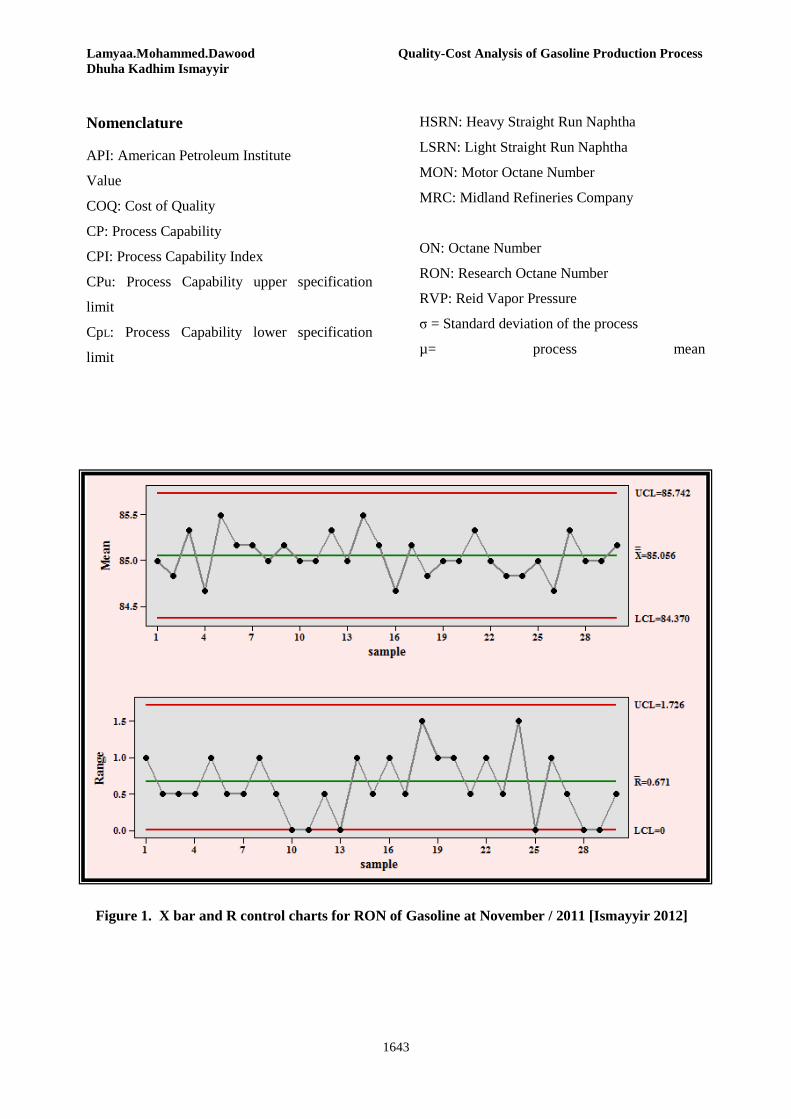
Lamyaa.Mohammed.Dawood Quality-Cost Analysis of Gasoline Production Process Dhuha Kadhim Ismayyir
1643
Nomenclature
API: American Petroleum Institute
Value
COQ: Cost of Quality
CP: Process Capability
CPI: Process Capability Index
CPu: Process Capability upper specification
limit
CpL: Process Capability lower specification
limit
HSRN: Heavy Straight Run Naphtha
LSRN: Light Straight Run Naphtha
MON: Motor Octane Number
MRC: Midland Refineries Company
ON: Octane Number
RON: Research Octane Number
RVP: Reid Vapor Pressure
σ = Standard deviation of the process
µ = process mean
Figure 1. X bar and R control charts for RON of Gasoline at November / 2011 [Ismayyir 2012]

Journal of Engineering Volume 19 December 2013 Number 12
1644
Figure 3. Capability Analysis for RON Parameter in September/2011
Figure 4. Capability Analysis for RON Parameter in October/2011
Freq
uenc
y
Freq
uenc
y
Figure 2. Data Entry Window of RON at September / 2011

Lamyaa.Mohammed.Dawood Quality-Cost Analysis of Gasoline Production Process Dhuha Kadhim Ismayyir
1645
Table 1. Iraqi Marketing Specifications of Gasoline (2000) / Ministry of Oil [www.mrc.oil.gov.iq]
Parameters Regular Premium Super
Distilled @ 100º C Vol % (min) 30 30 30
Distilled @ 145º C Vol % (min) 70 70 70
Final Boiling Point ºC (max) 200 200 200
Color Yellow Red Red
RON (min) 85 91 96
Sulphur Content (wt %) (max) 0.05 0.05 0.05
Exist Gum (mg/ 100ml) (max) 4 4 4
Corrosion (copper strip) 1 1 1
Lead Content (gm/l) (max) 0.1 0.3 0.4
RVP (KPa/ cm²) @ 37.8 ºC 0.45-0.84 0.45-0.84 0.45-0.84
Specific Gravity @ 15.6 ºC 0.775 0.770 0.770
Figure 5. Capability Analysis for RON Parameter in November/2011
Figure 6. Capability Analysis for RON Parameter in December/2011
Freq
uenc
y
Fr
eque
ncy

Journal of Engineering Volume 19 December 2013 Number 12
1646
Table 2. Analysis of Gasoline production Conformance (September 2011 – December 2011)
Out of Specification Cp Cpk Month
2.4% 0.89 0.66 September
16.75% 1.4 0.32 October
44.42% 1.26 0.05 November
33% 1.32 0.16 December
Table 3. Quality-Costs Analysis of Gasoline Production Process
Table 4. Cost/Quality Loss Imparted to the Common Iraqi Customer
COQ/ M. ID Quantity loss due to lack quality (lit.)
Month
77.29 1944 September
722.8 14019.75 October
185 35980.2 November
142.4 27621 December
Cost loss by customer(M.
ID)
Monthly Out of Specification Quantity (lit.)
Production Quantity/month
(lit.)
Month
0.388800 1944 81000 September
6.583950 14019.75 83700 October
9.084960 35980.2 81000 November
5.524200 27621 83700 December

Journal of Engineering Volume 19 December 2013 Number 12
1647
3-D Map Producing for Groundwater Level using Kriging
Interpolation Method
Alaa Soud Mahdi Hussein Alwan Mahdi Rusul Khalid Tahir Assistant prof.at Remote sensing Unit Lect.at Surveying Dept. Msc. Student at Surveying Dept College of Sciences - Baghdad University College of Engineering Baghdad Univ. [email protected]. [email protected]. [email protected]
ABSTRACT:
Groundwater is one of the main water resources in the arid and semi arid areas. Due to increasing demand for water in different purposes these resource management is very important. Prediction of groundwater depth and elevation is useful for management of the scarce water resources.The application of the spatial statistical technique (kriging) is used in this study as estimation method, The data set consists of groundwater levels measured at about 43 wells were selected in the studied area in May 2010, in an area (1350) 𝑘𝑚2 a part of Baghdad City. With the use of measured elevations of the water table, experimental semivariograms were fitted into many models as linear, spherical, exponential and Gaussian semivariogram. The finally selected models were used to estimate groundwater levels and estimation variance (which express the accuracy of the estimated groundwater levels) to develop corresponding contour maps.
KEY WORDS: Kriging – Groundwater – Contour map – Cross-validation – semivariance – Variogram models.
إنتاج خارطة ثالثية االبعاد لمناسيب المياه الجوفية بأستخدام تقنية التخمين اإلحصائي (الكريكنك)
عالء سعود مهدي ، حسين علوان مهدي و رسل خالد طاهر
المستخلص:
في المتزايد على المياه المناطق الجافة وشبه الجافة، ونظرا للطلبفي موارد المياه البديلة أهم المياه الجوفية منتعتبرالمياه الجوفية عمقب التنبؤوعليه فإن مهمة جدا لكافة االستخدامات المدنية والزراعية. إدارة هذه المواردفإن أغراض مختلفة
في (kriging)تم في هذا البحث تطبيق تقنية التخمين االحصائي الكريكنك . ددارة تلك الموارإلمفيد ارتفاعها عن السطح وبئر مختارة في شهر 43اخذت مجموعة بيانات لمنسوب المياه الجوفية المقاسة حقليا من التخمين المكاني لمنسوب المياه الجوفية.
من نماذج) لعدة fittedلجزء من مدينة بغداد. تم عمل تقريب مالئم (كم مربع 1350في منطقة الدراسة لمساحة 2010الخامس )semivariograms) منها (Linear, Spherical, Gaussian and Exponential تم نماذج) وبعد إجراء االختبارات لعدة
لتخمبن مستوي المياه الجوفية في المنطقة وكذلك مقدار التباين ( الذي يعبر عن دقة التخمين النماذجالنهائي من هذه النموذجأختيار في منسوب المياه الجوفية ) ورسم خارطة كنتورية لمنسوب المياه الجوفية.
شبه – Cross validation طريقة –الكنتورية الخرائط –المياه الجوفية –طريقة التخمين االحصائي (الكريكنك) : الرئيسية الكلمات Variogramنماذج – التباين

Alaa Soud Mahdi 3-D Map Producing for Groundwater Level Hussein Alwan Mahdi using Kriging Interpolation Method Rusul Khalid Tahir
1648
AIM OF THE STUDY Using a kriging technique to estimate the groundwater levels within the study area (a part of Baghdad City), as well as study and create the hydrological map of ground water table in Baghdad city and finally producing 3-D map of groundwater levels. 1. INTRODUCTION Groundwater is one of the major sources of water. Management of this resource is very important to meet the increasing demand of water for domestic, agricultural and industrial use. Baghdad is the largest and most heavily populated city in Iraq. The nature of its groundwater is complex , because the water table is fluctuating among the year. In the recent years, there is a rapid growth of population, increasing municipal, industrial and agricultural activities, as well as the seepage from raw or treated water distribution network, in addition to the natural climate changes led to significant changes in ground water elevation periodically. Due to the above factors, it was difficult to create specific and accurate maps for groundwater, also collect the various data measured in one time was hard, beside the limited studies on this topic (absence of specific studies and maps) on the Baghdad water table. A part of Baghdad city was chosen with data of groundwater collected from observation wells which is the most important information sources for groundwater resources studying. Therefore, prediction of groundwater elevation, to create specific maps is useful to manage the groundwater in the study area.
2. GROUNDWATER ELEVATION MAP
Maps of water table elevation are a basic element of regional hydro geological investigations , they are used to identify the direction of groundwater flow and zones of recharge or discharge, to evaluate surface water, groundwater interactions and to assess the effect of natural or anthropogenic stresses on the groundwater system, [Desbarats et al., 2002].
Each water level measurement from a well or location of a surface water feature that was deemed to represent the water table at land surface was represented by a point (or set of points for some surface water features). These points represent the water table at these locations and can be used to interpolate the position of the water table between these points, [Snyder, 2008].
Geostatistical techniques play a vital role in sustainable management of groundwater system by estimating the model of regular grid points derived from random locations of measured points. Geostatistics is a collection of techniques that solved estimation problems involving spatial variables. It offers a variety of tools including interpolation, integration and differentiation of hydro geologic parameters to produce the prediction surface and other derived characteristics from measurements at random locations. Geostatistical techniques (such as kriging, co-kriging and universal kriging) have the capability of producing a prediction surface, and also provide some measure of capability of these predictions, [Kambhammettu et al., 2011].
The accuracy of the water table elevation maps depends on various factors: pertaining to the data, the method of interpolation, and the hydro geologic conditions of the surficial aquifers in the study area. The following assumptions are made with regard to the well data used for interpolation, [Snyder, 2008] :
• Water levels in wells are representative of water table conditions in unconfined aquifers;
• The median value of all water level measurements for each well is representative of the long-term position of the water table;
• Spatial positions of the wells are accurately known; • Land surface elevations of the wells are assessed
accurately; • The surface water features that were used for
interpolation were assumed to be the features that represent the long-term position of the water table as being present at land surface; spatial positions of the features are known accurately; and land surface elevations of the features are assessed accurately.
3. THE CASE STUDY
The study area lies in Baghdad city , restricted to latitudes between (33º 10′ - 33º 29′ N), and longitudes of (44º 09′- 44º33′ E), which located in the (UTM) lines follows: Latitude ( 3670300 – 3704442) and Longitude (420555 – 458534), with an area of about (1350 km2) approximately, The Tigris River passes through the city dividing it into two parts; Karkh and Rusafa. The area is bounded from the east by Diyala River which joins the Tigris River southeast of Baghdad. The Army Canal, 24 km long, recharges from the Tigris River in the

Journal of Engineering Volume 19 December 2013 Number 12
1649
northern part of the city and terminates in the southern part of Diyala River, [Al-Hiti, 1985].
For this study, groundwater level data pertaining to 43 wells in May 2010 (fig. 1) were selected, in addition to 14 monitoring wells (this wells within the 43 wells) were used to study the fluctuation of the water table during the period starting in (May 2010) to (April 2011), Table 1 shows the monitoring wells, [ALI, 2010]. The fluctuation of the water table at Rasafa side ranged from( 0.05 to 1.95) meter, whereas at Karkh the fluctuation ranged from (0.02 to 2.03) meter, The descriptive statistics of the observed groundwater levels for monitoring wells are shown in Table 2 and fig. 2
4. DERIVED DATA
It is obvious, the Tigers river divides the region into two parts. Therefore, the groundwater table estimation of the river was considered as boundary data. Tigris River elevation was calculated for each one kilometre based on elevation data on Sarai station ,the slope of the river in this region drops to about (7 cm/km), [AL-ANSARI, 1979].
Because the lack of data for Diyala River and Army Canal , the slope of them calculated by using mathematical operations. Their slopes were 10 cm/km , 11 cm/km respectively. The elevations of Diyala River and Army Canal was calculated for each one kilometer based on elevation of the Tigris River. The total number of points becomes 157 points (43 wells and 114 points of the surface water feature). The Universal Transverse Mercator (UTM) is the coordinate system used in locating the observation wells. The datum of this system is World Geodetic System of 1984 (WGS 1984). The primary results indicated that the observed data set were normal. Statistical specifications of the water table elevation of Baghdad city are presented in Table 3.
5. KRIGING METHOD Kriging is a group of geostatistical techniques to interpolate the value of a random field (e.g., the elevation, z, of the landscape as a function of the geographic location) at an unobserved location from observations of its value at nearby locations, the distance of every point pair is quantified to provide information on the spatial autocorrelation of the sample point set, [Muhsin, 2010].
In this study, ordinary kriging was evaluated as a procedure for interpolation water table elevation. Ordinary kriging is a linear estimator by which an estimated value of water table elevation in a particular site can be calculated, from water table elevation measured at other sites, according to the linear combination , eq. (5-1):
𝑧(𝑥𝑜) = ∑ 𝑤𝑖𝑛𝑖=1 𝑧(𝑥𝑖) (1)
Where Z is water table elevation, 𝑧(𝑥𝑜) is the estimated value of Z at point 𝑥𝑜, 𝑧(𝑥𝑖) is the measured value of Z at point 𝑥𝑖 , 𝑤𝑖 is the weight given to observed value 𝑧(𝑥𝑖). These weights are allowed to change as estimates are computed at different locations), 𝑥𝑜 is the coordinates [Universal Transverse Mercator (UTM)] of an estimated point, 𝑥𝑖 is the coordinates (UTM) of a measured value, and 𝑛 is the number of measured values used in the estimation. The weights 𝑤𝑖 are calculated using the ordinary kriging system of equations.
A common approach when solving the kriging system of equations is to employ what is called a semivariogram function 𝛾∗(ℎ). The experimental semivariance γ*(h) is estimated as, [Al-Mussawi, 2008] :
𝛾∗(ℎ) = 1
2𝑁(ℎ)∑ [𝑧(𝑥𝑖) − 𝑧(𝑥𝑖 + ℎ)]2𝑁(ℎ)𝑖=1 (2)
Where, 𝑁(ℎ) = the number of pairs separated by lag distance h; 𝑧(𝑥𝑖) = measured variable value at point i ; and 𝑧(𝑥𝑖 + ℎ) = measured variable value at point i+h.
Therefore, to use above equation to estimate semivariograms, data must be grouped into pairs with similar separation distances of about h (distance lags). Each lag contains N(h) number of pairs. Table 4 illustrated Semivariance values (experimental). Experimental semivariograms were calculated for 43 wells and 114 elevation point for surface water feature using the computer software (Geostatistics for the environmental sciences) Ver. (5.1).
There are two reasons for not using the experimental semivariogram directly in the ordinary kriging system. First, the kriging system

Alaa Soud Mahdi 3-D Map Producing for Groundwater Level Hussein Alwan Mahdi using Kriging Interpolation Method Rusul Khalid Tahir
1650
of equations may need semivariogram values for distances that are not present in the sample data; this requirement will depend on the location at which Z is being estimated. Second, the use of the experimental semivariogram does not guarantee the existence and uniqueness of the solution to the ordinary kriging system of equations.
Once the semivariogram function has been computed from the sampled values of Z at different locations, the next step is to fit a parametric semivariogram model to the experimental semivariogram γ*(h). The most common semivariogram models used to fit experimental semivariograms and therefore used to describe the spatial variability of the variable under study are Gaussian, spherical, exponential, and linear. Four commonly used variogram models are, [Robertson, 2008]:
• Spherical Model
𝛾(ℎ) = 𝐶𝑜 + 𝐶 �1.5 �ℎ𝑎� − 0.5 �ℎ
𝑎�3� (3)
• Exponential Model 𝛾(ℎ) = 𝐶𝑜 + 𝐶 �1− 𝑒𝑥𝑝 �−ℎ
𝑎�� (4)
• Linear Model 𝛾(ℎ) = 𝐶𝑜 + �ℎ �𝐶
𝑎�� (5)
• Gaussian Model
𝛾(ℎ) = 𝐶𝑜 + 𝐶 �1− 𝑒𝑥𝑝 �−ℎ2
𝑎2�� (6)
The parameters that characterize these
models are the nugget, sill, and range and are calculated through the fitting process. Fig. 3 illustrated semivariogram models and Table 5 indicate the properties of fitted semivariograms. The best semivariogram model was generated by observing the coefficient of determination (𝑟2) and residual sum square (RSS) values. The coefficient of determination (𝑟2) provides an indication of how well the model fits the variogram data ; highest 𝑟2 value ,the better the model fits. Residual Sum of Square (RSS) , provide an exact measure of how well the model fits the variogram data , the lower RSS ,the better the model fits.
The results in Table 5 indicate that best fitted semivariogram has spherical for the optimum model parameters (sill, nugget, and range) corresponding to the highest 𝑟2 and lowest RSS value were noted. Then from the best fit model fig. 3 (d), The theoretical fitted Spherical semivariogram for May 2010 data is of the form:
𝛾(ℎ) = 𝑜. 5 + 14.11 �1.5 � ℎ57810
� −
0.5 � ℎ57810
�3�
The covariance function is given by:
C(h) = C(0) − 𝛾(ℎ)= 𝑜. 5 + 14.11 �1.5 � ℎ57810
� −
0.5 � ℎ57810
�3�
The implementation of the ordinary Kriging method requires solving a huge number of equations, [Muhsin, 2010].
�𝑤𝑛∗1𝜆 � =
�𝐶{𝑧(𝑥𝑖),𝑧�𝑥𝑗�𝐾𝑇
𝐾0�(𝑛+1)∗(𝑛+1)
−1�𝐶{𝑍(𝑥𝑖),𝑍(𝑥𝑜)
𝐾𝑇 �(𝑛+1)∗1
(7)
Note: 𝐶�𝑑𝑖𝑗� = 𝐶�𝑑𝑗𝑖� ⇒ 𝐶�𝑧(𝑥𝑖), 𝑧�𝑥𝑗�� is symmetric
( ) ( ){ }( ) ( )
=+×+
011111}0{}3{}2{}1{
1}3{}0{}32{}31{1}2{}23{}0{}21{1}1{}13{}12{}0{
,11
CdnCdnCdnC
ndCCdCdCndCdCCdCndCdCdCC
xzxzCnnji
( ) ( ){ }( )
=×+
1}{
}3{}2{}1{
, 11
dnoC
odCodCodC
xzxzC noi

Journal of Engineering Volume 19 December 2013 Number 12
1651
𝑍(𝑥): vector, its height value of Ground Control Point (GCP); 𝐶�𝑧(𝑥𝑖), 𝑧�𝑥𝑗��: Covariance between ground control points with each other; 𝐶{𝑧(𝑥𝑖), 𝑧(𝑥𝑜)}: Covariance between ground control points with unknown point; And it is named 𝐶�𝑧(𝑥𝑖), 𝑧�𝑥𝑗�� and 𝐶{𝑧(𝑥𝑖), 𝑧(𝑥𝑜)} semi-variance. w : weighted value of the control points.
The minimum squared error estimation is also a measure for the accuracy of estimates, which is known as estimation variance, or kriging variance, and is given by,[ Al-Mussawi, 2008]:
𝜎𝑘2(𝑥𝑜) = ∑ 𝑤𝑖 𝑛𝑖=1 𝛾(𝑥𝑖, 𝑥𝑜) + 𝜆 (8)
Application this method have been used by GS+ software. Based on the obtained data values for study area from this method, the 3D-map of water table elevation was created, fig. 4.
6. CROSS VALIDATION The accuracy of the estimation was evaluated by cross-validation method (i.e. without additional data). In cross-validation analysis each measured point in the spatial domain is individually removed from the domain and its value estimated as though it were never there. The point is replaced and the next point is removed and estimated, and so on. In this way a graph can be constructed of estimated vs. actual values for each sample location in the domain, [Robertson, 2008]. In this case the transformed data were used for the calculation and the differences between estimated and sample values were expressed in two-dimensional diagrams fig. 5, with calculation of the regression coefficient, standard deviation and correlation coefficient (𝑅2), the regression coefficient represents a measure of the goodness of fit , a perfect 1:1 fit would have a regression coefficient of 1.00. While the correlation coefficient (𝑅2), which can summarize the correlation between the observed and estimated values. The distribution of errors was analysed using many of summary statistics: the mean error (ME), the mean absolute error (MAE), kriged reduced mean error (KRME) and kriged reduced mean square error (KRMSE), the error should satisfy the following criteria [MERINO et al., 2001]:
𝑀𝐸 = ∑ [𝑧∗(𝑥𝑖)−𝑧(𝑥𝑖)]𝑁𝑖=1
𝑁≅ 0 (9)
𝑀𝐴𝐸 = ∑ |𝑧∗(𝑥𝑖)−𝑧(𝑥𝑖)|𝑁𝑖=1
𝑁≅ 0 (10)
𝐾𝑅𝑀𝐸 = 1𝑁∑ ��𝑧∗(𝑥𝑖) − 𝑧(𝑥𝑖)� 𝜎𝑘⁄ �𝑁𝑖=1 ≅ 0 (11)
𝐾𝑅𝑀𝑆𝐸 = 1𝑁∑ ��𝑧∗(𝑥𝑖) − 𝑧(𝑥𝑖)�
2 𝜎𝑘2� �𝑁𝑖=1 ≅ 1
(12) Where, 𝑧∗(𝑥𝑖), 𝑧(𝑥𝑖) and 𝜎𝑘2 are the estimated value, observed value and estimation variance, respectively, at points 𝑥𝑖 . N is the sample size. As a practical rule, the MSE should be less than the variance of the sample values and KRMSE should be in the range 1±2√2/N.
Results of cross validation for may 2010 data with the fitted Spherical model resulted in a mean error (ME) of 0.11, (which is near to zero), mean square error (MSE) of 1.88, (which is very low as compared to the variance of the data ), kriged reduced mean error (KRME) of 0.0817, (which is very near to zero) and a kriged reduced mean square error (KRMSE) of 1.0002, (which is very near to 1 and within the range 1±2√2/N). The above cross validation results show that the chosen model and its parameters are adequate.
Groundwater levels and estimation variances were calculated by kriging for May of 2010. These estimated level values are used to draw the contour maps of groundwater levels and estimation variance. Fig. 6 and 7 are shown the contour maps of the groundwater levels and estimation variance obtained for May 2010 respectively. Fig. 7 can be interpreted as the map of the reliability of the kriged ground water level in Fig. 6. As seen from the Fig. 7, the estimation variance is low at 1.5 𝑚2 in the middle and southeast of the study area (where most of the observation points are located) and increase rapidly towards the boundaries, where no observation well is located. 7. CONCLUSIONS
In this study, kriging, a type of geostatistical techniques, is applied to the groundwater level data of May 2010, The Spherical model is found to the best model was generated by observing the coefficient of correlation (highest 𝑟2) and

Alaa Soud Mahdi 3-D Map Producing for Groundwater Level Hussein Alwan Mahdi using Kriging Interpolation Method Rusul Khalid Tahir
1652
residual sum square (lowest RSS). Groundwaterer levels in the part northeast of Baghdad city are highest results of high population density as well as the seepage from raw or treated water distribution network. The result of the groundwater level maps showed that groundwater level has declined in central (toward the surface water feature) of the study area. The estimation variance is low at 1.5 𝑚2 in the middle and southeast of the study area. The correlation between estimation and actual values was strong (R=0.81). REFERENCES Al-Hiti B.M., (1985) , “Ground water quality within Baghdad area”, M.Sc. Thesis, University of Baghdad. ALI S. M., (2012), “ Hydrogeological Environmental Assessment Of Baghdad Area”, Ph.D. Thesis presented to the University of Baghdad, College of Science, . Al-Mussawi W. H. , (2008) “ Kriging of Groundwater Level - A Case Study of Dibdiba Aquifer in Area of Karballa-Najaf” , Journal of Kerbala University , Vol. 6 No.1 Scientific . AL-ANSARI N. A., ALI S. H. and TAQA A. S., (1979), “Sediment discharge of the River Tigris at Baghdad (Iraq)”, The hydrology of areas of low precipitation, Proceedings of the Canberra Symposium, no. 128 December.
Desbarats A. J., Logan C. E., Hinton M. J. and Sharpe D. R., (2002), “On the kriging of water table elevations using collateral information from a digital elevation model”, Journal of Hydrology vol. 255. Kambhammettu B., Allena P. and King J. P., (2011), “Application and evaluation of universal kriging for optimal contouring of groundwater levels”, Indian Academy of Sciences, Journal of Earth Syst. Sci. vol. 120, No. 3 . Muhsin I. J. , (2010), “ High Resolution Digital Elevation Model (DEM) for University of Baghdad Campus”, PhD. Thesis, University of Baghdad, College of science. MERINO G. G. , JONES D. , STOOKSBURY D. E. and HUBBARD K. G. , (2001), “Determination of Semivariogram Models to Krige Hourly and Daily Solar Irradiance in Western Nebraska”, Journal of the Nebraska Agricultural Experiment Station, American Meteorological Society, No. 12746.
Robertson, G. P., (2008), “ GS+: Geostatistics for the Environmental Sciences”, Gamma Design Software, Plainwell, Michigan USA. Snyder D. T., (2008), “Estimated Depth to Ground Water and Configuration of the Water Table in the Portland, Oregon Area”, U.S. Geological Survey Scientific Investigations Report 5059.

Journal of Engineering Volume 19 December 2013 Number 12
1653
Table (1): Groundwater level fluctuation of the monitoring wells
Well No.
May. (5)
Jun. (6)
Jul. (7)
Aug. (8)
Sept. (9)
Oct. (10)
Nov. (11)
Dec. (12)
Jan. (1)
Feb. (2)
Mar. (3)
Apr. (4)
W7 35.61 35.68 34.71 35.28 35.21 35.63 35.73 35.83 35.88 35.83 35.88 35.88 W16 31.94 31.74 31.49 31.49 31.59 31.59 31.84 31.94 31.99 31.94 31.79 31.89 W17 28.64 28.59 28.44 28.64 28.54 28.24 28.84 28.44 28.64 28.34 28.49 28.64 W19 32.20 31.60 31.15 31.60 30.62 30.25 31.55 31.35 31.55 31.30 31.80 31.90 W21 32.80 32.52 32.60 32.60 32.70 32.61 32.91 33.25 33.40 33.55 33.60 33.50 W24 33.36 33.15 33.05 33.40 33.40 33.30 32.97 33.20 32.75 32.50 33.30 33.40 W25 33.12 31.79 31.09 31.19 31.24 31.29 31.41 31.98 32.34 32.31 32.49 32.49 W28 30.75 30.42 29.92 30.52 30.57 30.47 30.57 30.95 30.97 30.92 30.87 30.82 W29 29.94 29.22 28.87 28.54 29.02 29.12 29.52 29.42 29.62 29.67 29.92 30.12 W32 32.37 32.22 32.17 32.02 32.07 31.97 32.07 32.42 32.47 32.52 32.42 32.42 W34 29.57 29.55 29.47 29.47 29.37 29.17 29.27 29.47 29.37 29.37 29.27 29.32 W35 31.00 29.60 29.66 29.70 29.90 29.80 29.65 29.57 29.40 29.75 29.95 30.75 W39 31.47 31.57 31.32 31.47 31.62 31.67 31.72 31.97 31.86 31.57 31.27 31.62 W41 30.59 30.44 30.19 29.49 29.84 29.89 30.09 30.49 30.64 30.74 30.79 30.79
Table (2): Descriptive statistics of the Monitoring wells
Well No.
Max. G.W. Min. G.W. Diff Elv. In (m.) Remarks
Elv. Date Elv. Date W7 35.88 (1) Jan. 34.71 (7) Jul. 1.17 Max. In (1),(2),(3),(4) W16 31.99 (1) Jan. 31.49 (7) Jul. 0.50 Max. In (1),(2),(3),(4) W17 28.84 (11) Nov. 28.24 (10) Oct. 0.60 W19 32.20 (5) May. 30.25 (10) Oct. 1.95 W21 33.60 (3) Mar. 32.52 (6) Jun. 1.08 W24 33.40 (4) Apr. 32.50 (2) Feb. 0.90 Max. In (8),(9),(4) W25 33.12 (5) May. 31.09 (7) Jul. 2.03 W28 30.97 (1) Jan. 29.92 (7) Jul. 1.05 Max. In (1),(2),(3),(4) W29 30.12 (4) Apr. 28.54 (8) Aug. 1.58 W32 32.52 (2) Feb. 31.97 (10) Oct. 0.55 Max. In (1),(2),(3),(4) W34 29.57 (5) May. 29.17 (10) Oct. 0.40 W35 31.00 (5) May. 29.40 (1) Jan. 1.60 W39 31.97 (12) Dec. 31.27 (3) Mar. 0.70 W41 30.79 (4) Apr. 29.49 (8) Aug. 1.30 Max. In (1),(2),(3),(4)
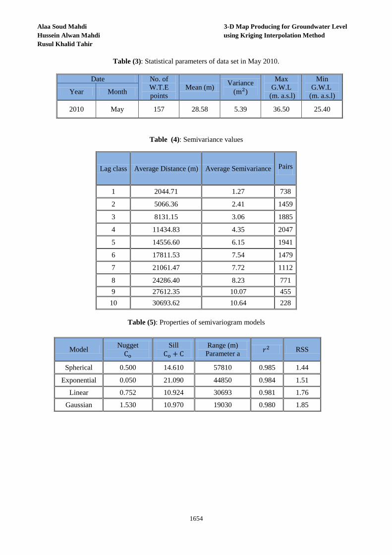
Alaa Soud Mahdi 3-D Map Producing for Groundwater Level Hussein Alwan Mahdi using Kriging Interpolation Method Rusul Khalid Tahir
1654
Table (3): Statistical parameters of data set in May 2010.
Date No. of
W.T.E points
Mean (m) Variance (m2)
Max G.W.L
(m. a.s.l)
Min G.W.L
(m. a.s.l) Year Month
2010 May 157 28.58 5.39 36.50 25.40
Table (4): Semivariance values
Lag class Average Distance (m) Average Semivariance Pairs
1 2044.71 1.27 738
2 5066.36 2.41 1459
3 8131.15 3.06 1885
4 11434.83 4.35 2047
5 14556.60 6.15 1941
6 17811.53 7.54 1479
7 21061.47 7.72 1112
8 24286.40 8.23 771 9 27612.35 10.07 455
10 30693.62 10.64 228
Table (5): Properties of semivariogram models
Model Nugget Co
Sill Co + C
Range (m) Parameter a 𝑟2 RSS
Spherical 0.500 14.610 57810 0.985 1.44
Exponential 0.050 21.090 44850 0.984 1.51
Linear 0.752 10.924 30693 0.981 1.76
Gaussian 1.530 10.970 19030 0.980 1.85

Journal of Engineering Volume 19 December 2013 Number 12
1655
Figure ( 1 ): Digital map of the study area and location of observation wells.

Alaa Soud Mahdi 3-D Map Producing for Groundwater Level Hussein Alwan Mahdi using Kriging Interpolation Method Rusul Khalid Tahir
1656
Figure (2): The fluctuation of (W.T.) levels

Journal of Engineering Volume 19 December 2013 Number 12
1657
(a) (b)
(c) (d)
Figure ( 3 ): Semivariogram models: (a) exponential; (b) Linear; (c) Gaussian and (d) Spherical.

Alaa Soud Mahdi 3-D Map Producing for Groundwater Level Hussein Alwan Mahdi using Kriging Interpolation Method Rusul Khalid Tahir
1658
Figure (4): A 3-D map of G.W.T. visualizing the spatial distribution of the water table.
Figure (5): Cross-Validation for kriging.

Journal of Engineering Volume 19 December 2013 Number 12
1659
Figure (6): Groundwater level contours maps of the study area (m) .

Alaa Soud Mahdi 3-D Map Producing for Groundwater Level Hussein Alwan Mahdi using Kriging Interpolation Method Rusul Khalid Tahir
1660
Figure (7): Estimation variance (𝑚2) by Kriging .

Journal of Engineering Volume 19 December 2013 Number 12
1661
Removal of Hexavalent Chromium from Aqueous Solutions by Adsorption on Thermally Modified and Non-Modified Eggshells
Asst. Lect. Suheila abd alreda akkar Department of Chemical Engineering
College of Engineering- Baghdad University Email: [email protected]
ABSTRACT:
Removal of heavy metals from waste water has received a great deal of attention. The compare Cr (VI) adsorption characteristics removing from wastewater by using thermally modified and non-modified eggshells were examined. Adsorption experiments were carried out in a batch process and various experimental Parameters such as effect of pH, adsorbent dosage, contact time, and initial chromium ion concentration on percentage removal have been studied. The modification of eggshells obtained by calcination which was performed in a furnace at 800ᵒC for 2h after crushing of the dried eggshells. The adsorption of chromium ions from solutions containing different initial 𝐶𝑟+6 concentrations (50,100,150) mg/L. The results show that all factors have a significant effect on the percentage removal of 𝐶𝑟+6 ions from aqueous solutions and the optimum pH, weight and time of treatment are (8, 5.8), (0.5, 0.01) g and (120 ,60 ) min respectively for non-modify and modify eggshell. The present study was also aimed to evaluate the equilibrium of adsorption process using Langmuir and freundlich isotherms. The Langmuir isotherm was the best for correlation of adsorption data, showing maximum capacities of 16.6 and 159 mg/g for non-modified and modified eggshells, respectively. Meanwhile, the kinetics of (𝐶𝑟+6) adsorption on eggshell and modified of eggshells also analyzed using pseudo-first order.
Key words: Waste Eggshells; CaO; Adsorption; Removal of 𝐶𝑟+6
المعالجه وغير بقشور البيضمتزازه ازالة ايون الكروم السداسي من المحلول المائي بواسطه ا المعالجه حراريا
رسهيله عبد الرضا عكام.م
كلية الهندسة/ جامعة بغداد/ قسم الهندسه الكيمياويه
الخالصه
حيث سوف يتم مقارنه بين ازالة ايون الكروم السداسي بواسطة قشور البيض المعالجه ازالة المعادن الثقيلة من الماء والمياه الملوثه حظيت باهتمام كبير،وجيني، وزن الماده المازه، ها دراسه المعامالت التاليه االس الهيدروغير المعالجه حراريا من الماء الملوث . واجريت التجارب في منظمومه دفعيه وتم في
يتم معالجه وتطوير قشور البيض بواسطه عمليه الكلسنه وذلك بادخال قشور البيض الى الفرن بدرجه زمن الخلط وتركيز االولي وتاثيرها على نسبة االزالة.امتزاز ايونات الكروم من المحاليل التي تحوي تراكيز بدائية مختلفة وسحق وطحن قشور البيض.درجه سيلزيه ولمده ساعتين وذلك بعد تجفيف 800حراره
ان الظروف المثالية للتخلص من ايون الكروم السداسي هو عند اس هيدروجيني ، وزن الماده وقد اثبتت النتائج ) ملغم/لتر50,100,150من الكروم (وفي هذا .) دقيقه على التوالي بالنسبه لقشور البيض غير المعالجه والمعالجه حراريا120,60) غرام، (0.01، 0.5)، (8,5.8المازه،والزمن هي االتي(
ملغم/غم )16.6,159سعة هي ( وقد اظهرت النتائج ان لونك ماير مطابقة للنتائج العمليه اعلى تحليل االيزوثيرم باستخدام لونك ماير والفريندلشالدراسة تم النماذج الحركيه فاستخدمنا البسيدو من الدرجه االولى لتحليل النتائجلقشور البيض المعالج وغير المعالج بالتتابع اما
الكلمات الرئيسيه: قشور البيض، اوكسيد الكالسيوم، االمتزاز، ازاله ايون الكروم

Suheila abd alreda akkar Removal of Hexavalent Chromium from Aqueous Solutions by Adsorption on Thermally Modified and Non-Modified Eggshells
1662
1. INTRODUCTION
Industrial waste water contaminated with heavy metals is commonly produced from many kinds of industrial processes therefore, if this waste water is not treated with a suitable process, it can cause a serious environmental problem in the natural eco-system [Ayad,2012 et al, park heung,et al. 2007].
Tannery effluent is a major source of aquatic pollution in Iraq with high hexavalent chromium. There are a large number of tanneries scattered all over Iraq. But the main areas of their concentration are al-qa`im ,haditha and hit and also in Baghdad in Al-Nahrawan .[Mohammed Nsaif, et al. 2013].
Water of high quality is essential to human life and of acceptable quality is essential for agriculture industrial, domestic and commercial uses. All these activities are also responsible for polluting the water. Billions of gallons of waste from all these sources are thrown to fresh water bodies every day [Muhammed Ali et al., 2012].
The requirement for water is increasing while slowly all the water resources are becoming unfit for use due to improper waste disposal [Suresh, et al. 2013]. The task of providing proper treatment facility for all polluting sources is difficult and also expensive; hence there is pressing demand for innovative technologies which are low cost, require low maintenance and are energy efficient [Rajendran, A. et al. 2011]. The adsorption technique is economically favorable and technically easy to separate as the requirement of the control system is minimum [Renge V.C et al., 2012].
Hexavalent chromium [Cr(VI)] compounds are being used in a wide variety of commercial processes and unregulated disposal of the chromium containing effluent has led to the contamination of soil, sediment, surface and ground waters. In trace amounts, chromium is considered an essential nutrient for numerous organisms, but at higher level, it is toxic and
mutagenic. Nearly 80% of the tanneries are engaged in the chrome tanning processes. Most of them discharge untreated wastewater into the environment. In such aqueous waste, Cr (VI) is present as either dichromate 𝐶𝑟2𝑂7−2 𝑖𝑛 acidic environments or as chromate (𝐶𝑟𝑂4−1) in alkaline environments. Chromium compounds were employed in textile coloring and leather tanning processes. The principal chromium emissions into surface waters are from metal finishing processes such as electroplating, pickling and bright dipping [Rajendran, 2010].
ollution of soils occurs as a result of the dumping of chromate wastes such as those from tanneries or electroplating and from sewage sludge disposal on land [Ambasht, 1983]. Uncontrolled emissions have greater potential for contaminating the fresh waters with relatively toxic form of Cr (VI), which exist only as oxy species and is strongly oxidizing other small discharges of Cr (VI) are from the additive in circulating waters, laundry chemicals [Anandakrishnanadar et al., 1992].
In this article, the technical feasibility of low cost (adsorption) , and locally available adsorbent (eggshell) for heavy metal removal (𝐶𝑟+6), from contaminated water has been reviewed.
This work is intended to remove Cr (VI) from aqueous solutions onto eggshells as an effective and low-cost. This also represents a serious problem for egg processing industries due to stricter environmental regulations and high landfill costs. Therefore, this paper aimed to present eggshells as porous adsorbents since it is feasible to grind the eggshell agro waste in the preparation of fine powders, which might pave the way for available materials. Moreover, Cr (VI) were successfully removed from water samples under the recommended conditions.
In the present investigation, to estimate the
amount of chromium ions present in its aqueous solutions after treatment and the removal of

Journal of Engineering Volume 19 December 2013 Number 12
1663
chromium from wastewater using eggshell as an adsorbent is attempted. Though many conventional adsorbent are used for the effective removal of heavy metal ions, egg shell has been chosen as adsorbents with an aim to use waste pollutant material as adsorbent.
The present work is also aimed at fixing the optimal conditions such as, pH, equilibrium time (for batch mode technique), dosages of adsorbent and initial concentration on the adsorption efficiency of (𝐶𝑟+6) from waste water by non-modified eggshells and modify eggshells besides for effective removal of chromium. To evaluate the equilibrium of adsorption process using Langmuir and freundlich isotherms. Meanwhile, the kinetics of (𝐶𝑟+6) adsorption on eggshell and modify of eggshells also analyzed using pseudo-first order kinetic models.
2. EXPERIMENTAL WORK
2.1 Preparation of Adsorbent.
Chicken eggshells were collected. To remove impurity and interference material such as organics and salts, the sample was rinsed several times with deionized water. Then the sample was dried at 100ᵒC for 24 h in the dry oven after that, the inner thin layer was removed from dried eggshell by hand. Then crushing eggshells were ground to a powder in a grinder, and sieved to obtain under 75µm size particles. Thermal modification of eggshells by calcination was performed in a furnace at 800 ᵒC for 2h. After calcination the structure has been change and much developed pore was observed from the emission of 𝑐𝑜2 . The formation of 𝑐𝑜2 was assumed to follow an endothermic reaction as described in reaction (1).
𝑐𝑎𝑐𝑜3 cao+𝑐𝑜2 (1)
The sample were then packed into desicater for future use.
2.2 Preparation of Metal Solutions.
A stock solution of chromium (VI) is prepared by dissolving 2.8287g of potassium dichromate
(𝑘2𝑐𝑟2𝑜7) in 1000 ml of distilled water. This solution is diluted as required to obtain standerd solutions containing (50, 100, 150) mg/L of chromium (VI).
The pH was adjusted with 0.1M NaOH and 0.1M Hcl solution and measured by pH meter.
The concentration of chromium (VI) ions in the effluent was determined spectrophotometrically by developing a purple-violet color with 1, 5-diphenyl carbazide in acidic solution as an complexing agent. The absorbance of the purple-violet colored solution is read at 540 nm after 10 min.
3. RESULTS and DISCUSSION
3.1 Equilibrium Study
To select optimal operating conditions for full-scale batch processing. The graph plotted in Fig.1 shows that a contact time of 120 min was sufficient to achieve equilibrium and that the adsorption did not change significantly with further increases in the contact time. Therefore, the removal of chromium concentrations at the end of 120 min are given as the equilibrium values of non-modify eggshell.
It is evident that time has significant influence on the adsorption chromium ion Fig.2 till 60min, the percentage removal of chromium ion. from aqueous solution increases rapidly and reached up to 99% for modify eggshell. A further increase in contact time has neglected effect on the percentage removal. When compare Fig.2 with Fig.1 the modify eggshell can remove the chromium ion (𝐶𝑟+6) through 10 min with (99%) percentage removal of (𝐶𝑟+6) of 50 mg/L concentration of𝐶𝑟+6. While the non-modify eggshell can remove 72% at the same time. The adsorption efficiency of chromium ions can be calculated as:
Removal percentage= ((Cₒ-Ce)/Cₒ)*100 (2)
Where Cₒ is the adsorbent initial concentration (mg/L), Ce is the adsorbent concentration at equilibrium (mg/L).

Suheila abd alreda akkar Removal of Hexavalent Chromium from Aqueous Solutions by Adsorption on Thermally Modified and Non-Modified Eggshells
1664
3.2 Effect of pH Value on Adsorption.
The pH of aqueous solution is an important controlling parameter that strongly affects the adsorption of metals on the surface of eggshells. All batch experimental were conducted at room temperature (25ᵒC). The results depicted in Fig. 3 illustrate that the maximum adsorption removal was attained at pH of 8. The distribution of species clearly indicates that between pH values of 2 and 4, the complex compound is adsorbed on eggshell, but that between pH values of 4 and 6, chromium is adsorbed principally, through cation exchange mechanism.
At pH 3, adsorption can be explained by ion-exchange mechanism in which the important role is played by carbonate groups that have cation-exchange properties, as has been reported. At lower pH < 3, the metal adsorption was diminished which may be attributed to the fact that protons compete with metal ions for carbonate binding sites. The concentration of protons is higher, and thus more groups are bound with protons and therefore less groups are available to metal ions. Moreover, the large part of eggshell sorbent was dissolved.
At pH 8 adsorption removal reached a maximum. The decrease in the removal efficiency at high pH values more than 8 may be attributed to the fact that the negative species of chromium are not capable of combination with the negative surface of eggshell.
While Fig.4 shows that adsorption removal of 𝐶𝑟+6of modify eggshell that optimum PH 5.8. as the PH increased the carbonate groups in chicken eggshells would be exposed increasing the negative charge on the adsorbent surface, attracting the metal cations and allowing the adsorption onto the adsorbent surface.
3.3 Effect of Adsorbent Dosage on Adsorption.
The effect of non-modify eggshells dosage on remove chromium ion is shown in Fig. 5. The removal increased from 30.8%, 41%, and 58% for different concentration (150, 100, 50) mg/L respectively to55%, 60%, and 80% with an
increase in adsorbent dosage from0.01 g to 1 g at pH = 8. However, no more significant removal of 𝐶𝑟+6 was observed by addition of more than 0.5 g of non-modify eggshell.
The effect of adsorbent dosage for modify eggshell on the adsorption of chromium (VI) process is shown in Fig. 6. Removal of chromium (VI) increases with increase of adsorbent dosage. The percentage removal increases from 56%, 74%, and 80.3% to 88%, 90%, and 99.9% for the concentration (150, 100, 50) mg/L respectively by increasing the adsorbent dosage from 0.005 to 0.05 g. the optimum dosage is (0.01) g. 3.4 Adsorption Isotherm.
A series of solutions containing different initial concentration of 𝐶𝑟+6ions in the range of (50-200) mg/L was prepared and employed for batch adsorption studies at 25 ᵒC and these flasks were placed on a shaker along 24h with 50 ml and 0.3g, pH of 8 of non-modify eggshells and 0.03 g, pH 5.8 of modify eggshells, Fig.7 and Fig.8 show the isotherm of non-modify and modify eggshells respectively.
The amount of adsorption at equilibrium qe (mg/g) was calculated as:
qe =(Cₒ-Ce)*v/w (3)
where Ce(mg/L)is the concentration of 𝐶𝑟+6solution at equilibrium and Cₒ is initial concentration of 𝐶𝑟+6. V (L) is the volume of the solution and w (g) is the mass of dry adsorbent used.
The equilibrium study is important for an adsorption process as it shows the capacity of the adsorbent and the adsorption isotherm is normally applied to describe the adsorption mechanism for the interaction of cations on the adsorbent surface.
In the present study, experimental data were analyzed using Langmuir and Freundlic models. The equations for Langmuir and freundlich isotherms are expressed as eq.4 and eq.5 respectively.

Journal of Engineering Volume 19 December 2013 Number 12
1665
𝑞𝑒 = 𝑞𝑚∗𝑘𝑙∗𝐶𝑒1+𝑘𝑙∗𝐶𝑒
(4)
𝑞𝑒 = 𝑘𝑓 ∗ 𝐶𝑒1/𝑛 (5)
Where qe is the adsorption capacity at equilibrium (mg/g), Ce is the adsorbent concentration at equilibrium (mg/L),kl is the adsorption equilibrium constant (L/mg) related to the apparent energy of adsorption, qm is the maximum adsorption capacity of adsorbent(mg/g), n indicates the bond energies between metal ion and adsorbent, and kf(L/g) is related to bond trength [Ghazy S.E.,2008,Zeid,2007].The Langmuir and freundlich equations represent 𝐶𝑟+6adsorption by non-modify and modify eggshells as illustrated in Fig.9 and Fig.10.
The adsorption constants of Langmuir and freundlich equation s and their correlation coefficients (𝑅2) are presented in Table1.
3.5 Analysis of adsorption kinetics
The kinetic study of metal ion adsorption is important to give insight into the adsorption rate, provide information on the contact time required for considerable adsorption to take place and also the factors affecting or controlling the adsorption rate. In order to investigate the mechanism of 𝐶𝑟+6adsorption by non-modify and modify eggshells and potential rate controlling steps one of the most commonly used kinetic model, psedo-fist orderwas employed to evaluate the adsorption of 𝐶𝑟+6 . the equation for the pseudo-first order kinetic model can be represented by eq.5
𝐿𝑜𝑔(𝑞𝑒 − 𝑞𝑡) = 𝐿𝑜𝑔𝑞𝑒- 𝑘12.303
𝑡 (5)
Where qt is the adsorption capacity at time t (mg/g), k1 is the first order reaction rate constant (L/min) [Areej,2012].
First order models illustrated in fig.11. A comparison of reaction rate constants and 𝑅2 values estimated from pseudo first order for non-
modify and modify eggshells is presented inTable2.
CONCLUSIONS
The removal of 𝐶𝑟+6from waste water by using non-modify and modify eggshells has been investigatedl under several condition such as at different pH, different dosage and contact time.the optimum pH of 𝐶𝑟+6adsorption was found at pH of 8 for non-modify eggshells and 5.8 for modify eggshells. The optimum dosage was 0.5g for non-modify eggshells and 0.01g for modify eggshell. The optimum contact time is 60 min and 120 min for modify and non-modify eggshells the modify eggshells is butter than non-modify that the number of active binding sites increased by calcination. Eggshells waste cheap material and thus it would be convenient to use it in industrial waste water treatment plants.
After calcination, most composition of eggshells was transfer med to lime (CaO) as well as enlargement of pore and grain was observed.
These results strongly suggest plausible reuse of calcination eggshell in the treatment of waste water contaminated with heavy metal.
REFERENCES
Areej Dalf Abbas,2012,”Influence of operating condition on adsorption of lead(II) from contaminated water using different adsorbent”,Eng&Tech..Journal, vol.30.NO.6, 2012.
Ambasht, R.S. (1983). Ecological consideration of water pollution, Souvenir and abstract, National Conference on River pollution and Human Health. PP. 3-4. Ananthakrishna Nadar, P., Balasubramanian, N., Venkatachalam, T., Prabakaran, T.R. (1992). Pollution load of Cauvery river water. Journal. of Natcon. 42, 91-104. Ayad M. jebur almamoori*, fikrat m. hassana andthaer i. kassimb,2012,” impact of industrial waste water on theproperties of one major

Suheila abd alreda akkar Removal of Hexavalent Chromium from Aqueous Solutions by Adsorption on Thermally Modified and Non-Modified Eggshells
1666
drainage in the regionof the middle euphrates / iraq”, int. j. chem. sci.: 10(4), 2012, 1785-1798,issn 0972-768x
Ghazy S. E., A. A. El-Asmy and A. M. EL-Nokrashy,2008,” Separation of chromium(III) and chromium(VI) from environmental water samples using eggshell sorbent”, Indian Journal of Science and Technology ,Vol.1 No 6 (Nov. 2008).
Rajendran. A and C.Mansiya,2011,”Extraction of chromium from tannery effluents using waste eggshell material as an adsorbent”, British Journal of environment and climate change,1(2),44-52,2011
Rajendran, A. (2010). Applicability of an ionic liquid in the removal of chromium from tannery effluents: A green chemical approach, African journal of Pure and Applied Chemistry., 4(6), 100-103. Renge,V. C. S. V. Khedkar and Shraddha V. Pande, “Removal of heavy metals from waste water using low cost adsorbent” Sci. Revs. Chem. Commun.: 2(4), 2012, 580-584 ISSN 2277-2669 Muhammad Ali Zulfikar,Edeh Dieke Mariske,and Samitha Dewi Djajanti,”Adsorption of lignosulfonate compounds using powder eggshell”,Songklanakarin J.sci.Technol,34(3),309-316,May-Jun 2012
Mohammed Nsaif Abbas, Firas Saeed Abbas, Hala Husham Nussrat, Safaa Neamat Hussein, “Synthesis of Promoted Catalyst from Iraqi Rice
Husk Used as a Raw Material for Treating Tannery Wastewater”, Australian Journal of Basic and Applied Sciences, 7(2): 511-528, 2013,ISSN 1991-8178
Nuttawan Pramanpol and Nuttakan Nitayapat,2006,” Adsorption of Reactive Dye by Eggshell and Its Membrane”, Kasetsart J. (Nat. Sci.) 40 (Suppl.) : 192 - 197 (2006)
Nurul Aimi binti Rohaizar, Norhafizah binti Abd. Hadi, Wong Chee Sien,2013,”removal of cu(II) from water by adsorption on chicken eggshell”, International Journal of Engineering &Technology IJET-IJENS Vol:13 No:01,2013
Park Heung Jai, Jeong Seong Wook, Yang Jae Kyu, Kim Boo Gil3, Lee Seung Mok,” Removal of heavy metals using waste eggshell”, Journal of Environmental Sciences 19(2007) 1436–1441. Suresh Gupta and B V Babu,2013,”Adsorption of chromium (VI) by low-cost adsorbent prepared from tamarind seeds”Birla institude of technology and science, India,2013
Zeid A. Al Othman, Ali Hashem and Mohamed A.Habila,2007”kinetic,equilibrium and thermodynamic studies of cadmium(II) adsorption by modified agricultural wastes”,2007,adsorption ,13,41-51,2007.

Journal of Engineering Volume 19 December 2013 Number 12
1667
Fig.1 Effect of contact time on adsorption onto non-modify eggshell (w=0.5g, v=50ml, pH=8, T=25ᵒC)
Fig.2 Effect of contact time on adsorption onto modify eggshell (w=0.0.01g, v=50ml, pH=5.8, T=25ᵒC)
0
10
20
30
40
50
60
70
80
90
100
0 50 100 150 200 250
Rem
oval
%
time(min)
C0=50ppm
C0=100ppm
c0=150ppm
84
86
88
90
92
94
96
98
100
102
0 30 60 90 120 150
Rem
oval
%
time (min)
50 mg/L
100 mg/L
150 mg/L

Suheila abd alreda akkar Removal of Hexavalent Chromium from Aqueous Solutions by Adsorption on Thermally Modified and Non-Modified Eggshells
1668
Fig.3 influence of pH on percentage adsorption of 𝑪𝒓+𝟔 by non-modify eggshells (w=0.8g, v=50ml, t=120m)
Fig.4 influence of pH on percentage adsorption of 𝑪𝒓+𝟔 by modify eggshells (w=0.06g, v=50ml, t=60m)
0
10
20
30
40
50
60
70
0 2 4 6 8 10 12pH
50mg/L
100mg/L
150mg/L
40
55
70
85
100
2 3 4 5 6 7 8 9 10
Rem
oval
%
pH
50 mg/L
100 mg/L
150 mg/L

Journal of Engineering Volume 19 December 2013 Number 12
1669
Fig.5 Effect of dosage on adsorption of 𝑪𝒓+𝟔onto non-modify eggshell.
Fig.4 Effect of dosage on adsorption of 𝑪𝒓+𝟔on to modify eggshell.
0
10
20
30
40
50
60
70
80
90
0 0.2 0.4 0.6 0.8 1 1.2
Rem
oval
%
Dose (g)
50 mg/L
100mg/L
150 mg/L
40
55
70
85
100
115
0 0.01 0.02 0.03 0.04 0.05
Rem
oval
(%)
Dose (g)
50 mg/L
100 mg/L
150 mg/L
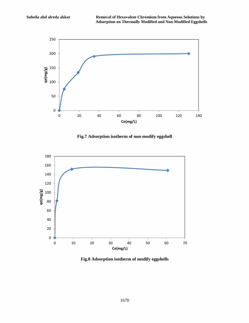
Suheila abd alreda akkar Removal of Hexavalent Chromium from Aqueous Solutions by Adsorption on Thermally Modified and Non-Modified Eggshells
1670
Fig.7 Adsorption isotherm of non-modify eggshell
Fig.8 Adsorption isotherm of modify eggshells
0
50
100
150
200
250
0 20 40 60 80 100 120 140
qe(m
g/g)
Ce(mg/L)
0
20
40
60
80
100
120
140
160
180
0 10 20 30 40 50 60 70
qe(m
g/g)
Ce(mg/L)

Journal of Engineering Volume 19 December 2013 Number 12
1671
Fig.9 Fitting curve for Langmuir for both modify and non-modify eggshells
Fig.10 Fitting curve for Freundlich for both modify and non-modify eggshells.
0
20
40
60
80
100
120
140
160
180
0 20 40 60 80 100 120 140
qe(m
g/g)
Ce(mg/l)
Langmuir egg
exp.egg
exp.modify egg
Langmuir modify egg
0
50
100
150
200
250
0 20 40 60 80 100 120 140
qe(m
g/g)
Ce(mg/l)
exp.modify eggshell
freundlich modify eggshell
exp.eggshell
freundlich eggshell

Suheila abd alreda akkar Removal of Hexavalent Chromium from Aqueous Solutions by Adsorption on Thermally Modified and Non-Modified Eggshells
1672
Fig.11 pseudo first order for non-modify and modify eggshells.
Table1. The Langmuir and freundlich isotherm constant
Langmuir model Freundlich model 𝑅2 qm (mg/g) kl(L/mg) n(g/L) Kf(g/g) 𝑅2
Non modify
0.97 16.6 0.099 4.08 65.1 0.8
Modify 0.98 159 8.008 95.3 0.9
Table2.kinetic constant for 𝑪𝒓+𝟔 adsorption by non-modify and modify eggshells
qe(mg/g) K1 𝑅2 Non-modify(50mg/g) 6.4027 0.0004 0.96 Non-modify(150mg/g) 9.6593 0.0031 0.94 Modify(50mg/g) 9.12 0.0001 0.99 Modify(150mg/g) 9.838 0.0007 0.99
4.2
4.4
4.6
4.8
5
5.2
5.4
5.6
0 50 100 150 200
Log(
qe-q
t)
time(min)
Exp.egg(50mg/L)
pseudo egg (50mg/L)
exp.egg(150mg/L)
Pseudo egg (150mg/L)
exp.modifyeggshell(50mg/L)
pseudo modifyeggshell(50mg/L)
exp.modifyeggshell(150mg/L)
Pseudo modifyeggshell(150mg/L)

Journal of Engineering Volume 19 December 2013 Number 12
1673
Analysis and Optimum Design of Self Supporting Steel Communication Tower
Assist. Prof. Dr. AbdulMuttalib I. Said, University of Baghdad, [email protected]
Ikhlass Hatto Hashim, M Sc. College of Engineering, University of Baghdad
ABSTRACT The present study deals with the optimum design of self supporting steel communication towers. A special technique is used to represent the tower as an equivalent hollow tapered beam with variable cross section. Then this method is employed to find the best layout of the tower among pre-specified configurations. The formulation of the problem is applied to four types of tower layout with K and X brace, with equal and unequal panels. The objective function is the total weight of the tower. The variables are the base and the top dimensions, the number of panels for the tower and member's cross section areas. The formulations of design constraints are based on the requirements of EIA and ANSI codes for allowable stresses in the members and the allowable displacement at antenna position. The Sequential Unconstrained Minimization Technique (SUMT) is used to perform the process. Direct stiffness method is used for the analysis of the structure, with beam elements. The strain energy is used to derive the stiffness matrix for members of unsymmetrical cross section. A computer program in FORTRAN is developed to represent the tower as an equivalent beam, and generate the tower nodes and members, analysis, design and to find the optimum design. Four types of tower are studied with different load cases. The effects of earthquake and wind loadings are taken in two directions and two positions of antenna are considered in the process to seek the optimum design. The tower type of X-brace with unequal panels has the minimum weight compared with other types of tower and the optimum design is satisfied when the angle of main leg is equal to (87O). KEYWORDS: Angle, Beam, Brace, Communication, Design, Optimum, Self supporting, Steel, SUMT, Tower, Wind.
البراج االتصاالت الحديدية المسندة تلقائياالتحليل والتصميم االمثل أ.م.د. عبد المطلب عيسى سعيد
حسام اخالص هاتوم.
الخالصة
تم تمثيل البرج بعتب مكافئ وناتئ يتعلق البحث بدراسة التحليل والتصميم االمثل البراج االتصاالت الحديدية المسندة تلقائيا. ومجوف ومتغير المقطع. تم ايجاد التصميم االمثل لهذا العتب واستغالل هذا التصميم اليجاد االبعاد الخارجية للبرج وعدد الخانات.
ساوية. بارتفاع خانات متساوية واخرى غير مت (K and X brace)اختيرت اربعة انواع من التشكيل والربط العضاء البرج هي

AbdulMuttalib I. Said Analysis and Optimum Design of Self Supporting Ikhlass Hatto Hashim Steel Communication Tower
1674
دالة الهدف هي الوزن الكلي للبرج ومتغيرات التصميم هي ابعاد القاعدة السفلى والعليا للبرج وعدد الخانات وابعاد مقاطع االعضاء االنشائية. محددات التصميم معتمدة على مقدار االزاحات المسموح بها عند مواقع المرسالت والمستقبالت وحدود االجهادات
ومواصفة (ANSI CODE)ء البرج وفقا للمعادالت التصميمية الخاصة بالمعهد االمريكي لالبراج الحديدية المسموح بها العضا اليجاد التصميم االمثل. (SUMT). استخدمت طريقة البرمجة غير المتعاقبة وغير المقيدة (EIA)جمعية الصناعات االلكترونية
واستعمال طاقة االجهاد الشتقاق مصفوفة الصالدة العضاء انشائية ذات استخدمت طريقة الصالدة في التحليل االنشائي للبرج
مقطع غير متناظر حول المحاور الرئيسية. تم كتابة برنامج بلغة فورتران ليقوم بتمثيل البرج بعتب ثم ايجاد التصميم االمثل لالبعاد رنامج بايجاد المقاطع الالزمة لالعضاء االنشائية.الخارجية واستحداث ملف يحتوي البيانات الالزمة للتحليل واخيرا يقوم الب
تمت دراسة االنواع االربعة من االبراج لحاالت تحميل مختلفة وهي تأثير الهزة االرضية وتأثير الرياح بزاويتين مختلفتين ولمواقع والرتفاع خانات غير متساوية. (X brace)مرسالت ومستقبالت مختلفة. لقد وجد ان اقل وزن للبرج يتحقق بتشكيل ربط من نوع
) درجة.87كما وجد ايضا ان التصميم االمثل يتحقق عندما تكون زاوية ميل البرج مساوية الى (
.البرمجة غير المتعاقبة وغير المقيدة ربط، اتصاالت، تصميم، امثل، مسند تلقائيا، حديد،، عتب، زاويةبرج، الكلمات الرئيسية:
1. STRUCTURAL ANALYSIS The structure of a communication tower consists of a large number of straight steel bars with constant cross section. Here the cross sections of the bars are equal leg angles. The self supporting communication tower is a large latticed steel structure and it should be analyzed as an indeterminate space structure. In this work, the analysis of the tower is made by using the linear elastic and standard stiffness method. For each member the equilibrium equations can be represented by the form: {P}= [K] {U} (1) Where {P} is the applied nodal load vector, which is for the space beam element {P}T={Fxl Fy1 Fz1 Mx1 My1 Mz1 Fx2 Fy2 Fz2 Mx2 My2 Mz2} [K] is the stiffness matrix of the member. {U} is the displacement vector, which is for beam element {U}T= [u1 v1 w1 θx1 θy1 θz1 u2 v2 w2 θx2 θy2 θz2] By assembling these equations for all members, the whole structure equilibrium equations are obtained. The equations can be solved for the unknown displacements, from which the internal forces can be obtained. A computer program is used to solve these equations.
1.1 Three-Dimensional Straight Beam Element A three dimensional prismatic beam element is considered, the beam is subjected to a general system of transverse loads and it is assumed to be linearly elastic. The element orientation with respect to local coordinate system and the nomenclature are illustrated in Fig.(1). The local x-y-z axes coincide with the centroidal axis of the element. Positive signs are in the directions indicated. The element has 12 degrees of freedom, six at each node. The forces and displacements at the two nodes are taken to be positive if their vectors points are in the directions of coordinates. The right-hand rule is used for moments and rotational displacements. Since the cross section of equal leg angles is not bisymmetrical the shear center dose not coincide with the centroid and consequently the stiffness matrix is somewhat different. 1.2 Effect of Axial, Torsion and Bending The total strain energy for axial, torsion and bending about two centroidal axes is: 𝑈 = ∫ {[ 1
2𝐸�𝐹𝑥𝐴
+ 𝑀𝑦𝑍𝐼𝑦
+ 𝑀𝑧𝑌𝐼𝑧�2
+ 𝑀𝑥2
2𝐺𝑗𝐿0 ]}𝑑𝑥 (2)

Journal of Engineering Volume 19 December 2013 Number 12
1675
The relationships between internal forces and the displacements of a point on the centroid of an unsymmetrical cross section of a straight member as given by Oden [1] are: Fx= EA u' (3) My= -EIyz v" –EIy w" (4) Mz=EIz v"+EIyz w" (5) Mx= GJ θx / L (6) From the above equations and by neglecting the small terms, the total bending strain energy Ub can be obtained as: 𝑈𝑏 = 𝐸
2 ∫ (𝐼𝑧. 𝑣" + 𝐼𝑦.𝑤"2 + 2𝐼𝑦𝑧.𝑤". 𝑣")𝐿0 𝑑𝑥
(7) where: Fx is the axial force, u is the axial deformation in the direction of x, My and Mz are the bending moments about y and z axes, v and w are the displacements in the directions of the principal axes y and z respectively, Mx is the torque, θx is the angle of rotation about x-axes, A is the cross sectional area, Iy and Iz are the moments of inertia, Iyz, is the product of inertia G is the modulus of rigidity and E is the modulus of elasticity, and Ix or J is the torsional constant which can be obtained as follow: For thin-walled open sections 𝐽 = 1
3∑𝑏. 𝑡3 and for
equal leg angle with cross section as shown in Fig.(2), where 𝐽 = 2𝑏𝑡3
3 (approximately). The
effect of each of these forces, which are axial, bending and torsion, is each separated from the others (i.e. uncoupled) when the stiffness coefficients are derived. 1.3 Shear Deformations The transverse shearing stress makes the cross section to warp in the longitudinal direction. The shear deformation is neglected because it is usually very small compared with those deformations due to bending. The convential beam theory is employed which assumes that plane sections remain plane in flexure, except in deep beams that have a usually large depth to span ratio (greater than 0.2) [1]. Due to the fact that all
members in the steel tower are not deep beams so the shear deformation is neglected 1.4 Warp Effect Torsional moments may cause longitudinal displacements resulting from the out of plane warping of the cross section. Torsional moments may cause longitudinal displacements resulting from the out of plane warping of the cross section. The equal leg angles twist without warping [1,2,3]. The shear center of the angle lays at the intersection of the centerlines of the thin rectangular strips. Because of this, the resultant of shear flows produced by any type of loading must pass through this point, hence no warping torque can be developed and no longitudinal stresses are produced by torsional loads. But, when the wall thickness t, is not extremely small compared with the other dimensions, a secondary stress system can be developed perpendicular to the contour line of the section. Normal stresses then vary linearly over (t) and secondary-warping torque is developed. However the largest value of thickness/width ratio for cross section of a commercial angle is close to (0.2), and this makes all effects from warping removed [2,3]. 1.5 Complete Element Stiffness Matrix The element stiffness matrix is found by using the approach of strain energy in terms of the nodal displacement of the element. By using Eq.7, the complete beam element stiffness matrix [K] in local coordinate system with 12 degrees of freedom, is derived as presented in Eq.8. To obtain the stiffness matrix for the entire structure, the usual transformation of each individual member stiffness matrix from the local to the global coordinates is needed.

AbdulMuttalib I. Said Analysis and Optimum Design of Self Supporting Ikhlass Hatto Hashim Steel Communication Tower
1676
1.6 Loading Cases In general there are two types of loading on the tower, dead load and live load. The live load consists of wind load and earthquake load. The dead load and wind load are calculated according to (EIA) standards [4], the wind load can be divided into two groups: (A): The wind load on the steel tower structure. (B): The wind load on the antennas. The full description of wind load calculation can be found in (EIA) Standard. While the earthquake loads are calculated according to Iraqi seismic code requirements for building (ISD) [5]. It is being noted that wind load is not considered in combination with seismic actions. (8) 2 Formulation of optimum design The purpose of this study is to develop an optimum design of a steel communication tower which is defined as the structure of least weight, subject to a prescribed set of constraints on the design and behavior variables. The problem is to design both the shape and the member sizes and locations. The problem can lead to mixed design variables, which, in turn, can have a wide range of sensitivities. The optimum design of a tower consists of shape and layout of tower, and the areas of the cross sections of the members. The optimum shape of the tower includes the horizontal dimensions along the height of the tower and the number of
panels and their height, where the configuration of the members is same at each panel. The optimum layout of a tower can be obtained by removing some members and not allowing re-entering the design problem. The member's having areas reduced to zero are removed during the process of optimization, while joints are moved until an optimum geometry for the given structure of the tower is found. In the case of removed members, there is no mathematical justification for the removal of these members and no proof exists that they would not subsequently help to reduce the weight of the structure. Furthermore, if the buckling stress constraint is critical for a particular member then its area would not reduce to zero in the design process and the member is not deleted. While in the case of moving the joints, some reasonable initial geometry is specified and it is difficult to estimate the best number of panels in a tower, since the joint move is simple, always in horizontal dimension. Most latticed towers may be built-up with angles at the corners and lacing in the faces as shown in Fig.(3). One alternative is to model the tower from three-dimensional truss or beam system to one or several equivalent beams is possible. The equivalent beam to a latticed tower is a beam having properties which give the same deflected shape to the tower and same axial stress in leg members under the same load conditions. The equivalent beam has the same base and top dimensions x2 and x1 respectively for the tower and the length of beam L represent the height of the tower. The equivalent beam and the tower have the same material properties. 2.1 Properties of Equivalent Beam In this study approximation concepts are made for the design of the tower to find the optimum layout, by modeling the tower as a tapering thin hollow square cantilever, whose section varies continuously from one end to the other. The beam has constant ratio of width/thickness, as shown in Fig. (4).The Y-axis coincides with the centroidal axis of the beam. The concept of constant CB ratio along the beam

Journal of Engineering Volume 19 December 2013 Number 12
1677
is due to the fact that the size of the member is reduced towards the top of the tower, also the dimension of the cross section of the tower. Writing the ratio of 𝑥1
𝑡1= 𝑥2
𝑡2= 𝑥(𝑦)
𝑡= 𝐶𝐵, then
x(y) = x1(1+ R.y) (9) Where: 𝑅 = 1
𝐿�𝑥2𝑥1− 1� (10)
Then the area at any section 𝐴 = 4𝑥(𝑦)2
𝐶𝐵, and the
moment of inertia can be given as: 𝐼𝑥(𝑦) = 𝐼𝑧(𝑦) = 𝐼𝑜(1 + 𝐵.𝑦) (11) Where I0= moment of inertia at y= 0 (top of tower). 𝐵 = 1
𝐿�𝑥2
4
𝑥14− 1� (12)
Every tower structure has a point of optimum economy, which depends primarily upon the dimensions at the base and top, and number of panels and number of members. The ratio CB is an indicator to the total volume of material of members used in the tower. In addition to that, the number of panels affects on the value of CB, and this effect is different when the panels are equal or not equal (having an algorithm relationship for height of panel as shown in Fig.(5). Writing TV be equal to the total volume of material in the actual tower (∑𝐴𝑖𝑙𝑖) and the CT to represent the material volume ratio, thus
𝐶𝑇 = 2𝐿(𝑥22+𝑥12)𝑇𝑉
(13)
Equation 13 is the same for any configuration system, for any number of panels of tower
with
square bases. Then CT for the equivalent beam can be represented in terms of CB: CT = f (CB, n) (14) Where n is the number of Panels.
Equation 14 is different for equal or unequal panels and configuration system. It can be obtained by analyzing a number of examples for each type. Then, TV = f (CT ,x2, x1) TV = f (CB x2, x1, n) Also there is a relation between the axial force FT in leg members in the actual tower and the force calculated due to allowable stress at the bottom of the equivalent beam FB. 2.2 Displacements in an Equivalent Beam The most important displacements in the tower are the axial (vertical) and transverse (horizontal) displacements at the top of the tower. The following sections explain the derivation of the displacements of the tapering hollow square beam: 2.2.1 Axial Displacement Mainly the axial (vertical) displacement (v) is caused by the se1f-weight of the structure. The vertical displacement at any distance (y) is due to the weight of the segment from origin (top of the tower) to distance (y) and it can be given as follows: 𝑓𝑦 = 2𝛾𝑠
𝐶𝐵 (𝑥12 + 𝑥𝑦2)𝑦 (15)
Where: γs: the weight density of steel. fy: is the vertical force in y-direction which is equal to the weight from the top to distance y. The differential equation of axial displacement of a straight bar is: 𝑑𝑣𝑑𝑦
= 𝑓𝑦𝐴.𝐸
(16) Where E: modulus of elasticity 𝑣(𝑦) = ∫ 𝑓𝑦
𝐴.𝐸 𝑑𝑦 (17)
The boundary condition is v=0 at y= L. By integrating Eq.16, the axial displacement can

AbdulMuttalib I. Said Analysis and Optimum Design of Self Supporting Ikhlass Hatto Hashim Steel Communication Tower
1678
represented as follows:
𝑣(𝑦) =𝛾𝑠2𝐸
⎣⎢⎢⎢⎢⎢⎡
1𝑅2
⎩⎪⎪⎨
⎪⎪⎧
ln(1 + 𝑅.𝑦) +ln(1 + 𝑅. 𝐿) +
1(1 + 𝑅.𝑦) +
1(1 + 𝑅. 𝐿) ⎭
⎪⎪⎬
⎪⎪⎫
+𝑦2
2+𝐿2
2
⎦⎥⎥⎥⎥⎥⎤
(18) 2.2.2 Transverse Displacement The transverse (horizontal) displacement in beam is u in x direction and w in z direction, which are the same for a symmetrical square tower. The differential equation of transverse displacement (u) or (w) is: 𝑑2 𝑢𝑑𝑦2
= −𝑀𝑧𝐸𝐼𝑧(𝑦)
(19) 𝑀𝑧 = −𝐸𝐼𝑧(𝑦) 𝑑
2 𝑢𝑑𝑦2
(20) The horizontal loads on the tower are concentrated loads (load on antenna) or uniform loads (wind loads), thus the derivation of displacement for concentrated and uniform loads are separately obtained. 2.2.2.1 Transverse Displacement under Uniform Load The differential equation of transverse displacement under uniform load is: 𝑑2 𝑀𝑧
𝑑𝑦2= 𝑑𝑉𝑥𝑑𝑦
= −𝑃𝑥
𝑑2 𝑑𝑦2
�−𝐸𝐼𝑧(𝑦) 𝑑2 𝑢𝑑𝑦2
� = −𝑃𝑥 (21) Where Vx shear force, & Px load intensity per unit length Px= Wx. x(y) (22) Where Wx load intensity per area in x direction.
𝑑2 𝑑𝑦2
�−𝐸𝐼𝑧(𝑦) 𝑑2 𝑢𝑑𝑦2
� = −𝑊𝑥.𝑥(𝑦) (23) The boundary conditions are:
𝑑3 𝑢𝑑𝑦3
=𝑑2 𝑢𝑑𝑦2
= 0 𝑎𝑡 𝑦 = 0
(zero shear and moment), and
𝑑𝑢𝑑𝑦
= 𝑢 = 0 𝑎𝑡 𝑦 = 𝐿
(zero slope and displacement) By integrating Eq.21, the transverse displacement is represented as follows:
𝑢(𝑦) =𝑊𝑥 . 𝑥1𝐸𝐼
⎣⎢⎢⎢⎢⎢⎢⎢⎢⎢⎢⎢⎢⎢⎢⎢⎡ 𝑅.𝑦4
72𝐵+ 𝑦3 �
−𝑅36𝐵2
−1
12𝐵� +
𝑦2 �−14𝐵2
+𝑅
12𝐵3� +
𝑦
⎩⎨
⎧−12𝐵3
+𝑅
6𝐵2−𝐿2
4𝐵+
𝐿2𝐵2
−
𝑅. 𝐿3
18𝐵+𝑅. 𝐿2
12𝐵2−𝑅. 𝐿6𝐵3
⎭⎬
⎫+
{𝑙𝑛(1 + 𝐵𝐿) − 𝑙𝑛(1 + 𝐵.𝑦)}.
�𝑅.𝑦6𝐵4
−𝑦
2𝐵3−
12𝐵4
−𝑅
6𝐵5� +
𝐿3
6𝐵−
𝐿2
4𝐵2+
𝐿2𝐵3
+𝑅. 𝐿4
24𝐵−
𝑅. 𝐿3
18𝐵2+𝑅. 𝐿2
12𝐵3+ 𝑅. 𝐿6𝐵4 ⎦
⎥⎥⎥⎥⎥⎥⎥⎥⎥⎥⎥⎥⎥⎥⎥⎤
(24) 2.2.2.2 Transverse Displacement under Concentrated Load The differential equation of transverse displacement under a concentrated load is: 𝑑2 𝑢𝑑𝑦2
= 𝑓𝑥(𝑦−𝑎)𝐸𝐼𝑧(𝑦)
(25) Where fx is the concentrated load at distance (a) from the origin, and (y-a) is Macaulay's brackets: (y-a) =(y-a) for y >a, and (y-a)= zero for y < a.

Journal of Engineering Volume 19 December 2013 Number 12
1679
The boundary conditions are:
𝑑𝑢𝑑𝑦
= 𝑢 = 0 𝑎𝑡 𝑦 = 𝐿
(zero slope and displacement) By integrating Eq.25 the transverse displacement can be represented as follows:
𝑢(𝑦) =𝑓𝑥𝐸𝐼𝑧
⎣⎢⎢⎢⎢⎢⎢⎢⎡
𝑦2
2𝐵− �
1𝐵2
+𝑎𝐵�
⎩⎪⎨
⎪⎧
𝑦. 𝑙𝑛(1 + 𝐵𝑦) −
𝑦 +𝑙𝑛(1 + 𝐵.𝑦)
𝐵−
𝑦. 𝑙𝑛(1 + 𝐵𝐿) +
𝐿 +𝑙𝑛(1 + 𝐵. 𝐿)
𝐵 ⎭⎪⎬
⎪⎫
−𝐿.𝑦𝐵
+𝐿2
2𝐵 ⎦⎥⎥⎥⎥⎥⎥⎥⎤
(26) The final equation for displacement in other direction (w) has the same statements for displacement (u) in uniform and concentrated load by replacing w, and fx by wx and fx respectively, since Ix= Iz for the square box section. 2.3 Representation of a Tower by an Equivalent Beam To find the properties of the equivalent beam which represents the tower, the relationship between CT with CB and FT with FB must be known for each type of configuration. These relations can be known by analyzing the tower with specific heights, x2, x1 layout, n, and cross section of the members. Then analyzing the hollow tapered beam with the same height of this tower, and same x2, and x1, to find the value CB, which gives the same deflected shape of the tower under the same load conditions. Here the tolerance for displacement should not exceed (0.5 %). This procedure is repeated for the number of panels and x2, and x1 for each type of configuration. The analysis of the actual tower is done by the use of beam elements. The analysis includes the leg members and main brace members (excluding the redundant members). The same things are used in the calculation of the value of TV.
Because of the large number of analysis procedure and the number of input data files needed, four programs in FORTRAN-77 language using Fortran Power Station 4.0 [7] are built to generate these data files. These programs just need dimensions of base and top and number of panels to generate the node numbers, the coordinates, the number of members, and the connectivity nodes. Also these programs can distribute the load on the tower according to the equations provided. Considering the number of examples with different dimensions at base and top and different number of panels with specific height, the relation between CT and CB and the relation between FT and FB for X-brace (Fig (6-a)) with equal panels are obtained, and they are shown in Fig.(7) and Fig.(8) respectively. These relations can be represented by the following equations: CT=136.5 -20.484 n +1.68 n2 -0.044 n3 + (0.153 + 0.03 n -0.0025 n2) CB FT=39.6 -9.24 n+ 0.7n2 -0.017n3+ (0.0106 -0.00262 n + 0.0002 n2) FB-0.0006 FB2 (27) The relation between CT and CB and the relation between FT and FB for X-brace with unequal panels, are shown in Fig.(9) and Fig.(l0) respectively. CT and FT can be represented by the following equations: CT=133 -13.56 n +1.123 n2 -0.03 n3 + (0.451 + 0.04 n -0.003 n2) CB FT=9.34-2.306n+0.2006n2-0.00573n3 +0.81 FB+(-0.0405 +0.01n-0.00085 n2)FB2
(28) For the tower of type K-brace (Fig. (6-b)) with equal panels, Fig. (11) and Fig. (12), explain the relation between CT and CB and the relation between FT and FB. The following equations represent the graph relationship: CT= 112.93 -12.83 n +1.09 n2 -0.031 n3 + (0.3 -0.014 n -0.00033 n2) CB FT= -8 +1.808n-0.15n2+0.004n3+ (1.245+

AbdulMuttalib I. Said Analysis and Optimum Design of Self Supporting Ikhlass Hatto Hashim Steel Communication Tower
1680
0.073n- 0.006n2 -0.00015n3 ) FB + (-0.0016 + 0.00024n) FB2 (29) For the tower of type K-brace and unequal panels configuration, Fig. (13) and Fig. (14) explain the relation between CT and CB and the relation between FT and FB, which can be represented by the following equations: CT=104 -11.67 n + 0.976 n2 -0.027 n3 + (0.064 + 0.06n2 -0.0054 n3 ) CB FT= -3.65 -0.98 n+ 0.08 n2 -0.0022 n3 + 0.9 FB + 1-0.0068 + 0.0015 n -O.000l2 n2) FB2 (30) 2.3.1 Verification Problems A tower of type X-brace with four equal panels which shown in Fig. (15 b) is subject to a number of load cases. The tower has dimensions (L=20m), (XB=6m), (XT=2m), and cross section area for leg members equal to (A=51.5 cm2) and, (A=23.5 cm2) for redundant members. The TV for this tower is (1.15m3), according to Eq.13 and (1396.) for CT. The equivalent tapering hollow square beam shown in Fig. (15 a) has CB equal to (5647). The results of analysis and load cases for the tower and the equivalent beam are shown in Table(1). The displacements at top and forces (at base) for the equivalent beam are calculated for the same CB so the tower can be represented by the equivalent beam. Table (1) Analysis results and load cases for the tower and the equivalent beam. Number of loading case in X-Dir. (kN) 1 2 3 Equiv. beam
at point
Tower at
node
Equiv. beam
at point
Tower at
node
Equiv. beam
at point
Tower at
node
a 0 1 0 a 6 1 0 a 0 1 0 2 0 2 0 2 0
b 0 3 0 b 6 3 3 b 4 3 2 4 0 4 3 4 2
c 0 5 0 c 6 5 3 c 6 5 2 6 0 6 3 6 2
d 10 7 5 d 6 7 3 d 8 7 2 8 5 8 3 8 2
No. of load case
Structure Type
Horizontal displacement at top (mm)
Axial force (kN)
1 Equivalent beam
1.2930235 18.75664
Tower 1.2929880 12.68638 2 Equivalent
beam 1.1786454 25.32147
Tower 1.1192827 13.070202 3 Equivalent
beam 1.4513451 27.19713
Tower 1.3785101 15.40162 2.4 Optimum Layout of Tower by Equivalent Beam The approach presented in the formulation of optimum layout of the tower is based on finding the optimum design of the equivalent beam and using its layout dimension for the layout dimension of the tower. There are many available methods of optimization, here the Sequential Unconstrained Minimization Technique SUMT method, [8, 9], is used. 2.4.1 The Objective Function The objective function to be minimized is the total weight of the equivalent beam W that is: W = γ TV (31) Where γ is the density of member material, which used in the tower. Since γ is constant for all the tower elements, hence the objective function to be minimized is TV, (TV=2L(x2
2 + x12)/CD. There
are three variables, direct variables (x2, x1) and indirect variable (n). CT is a function of CB and n. 2.4.2 Behavior Constraints 2.4.2.1 Displacement at Top Since the variation of the allowable horizontal displacements along the height of the tower is linear, the displacement at top is considered as the

Journal of Engineering Volume 19 December 2013 Number 12
1681
maximum i.e. the displacement at y=0. Therefore the displacement constraint will be as follow: 𝛾𝑠2𝐸
�1𝑅2
�ln(1 + 𝑅. 𝐿) + 1 +ln(1 + 𝑅. 𝐿) � +
𝐿2
2� ≤
Allowable vertical displacement at top.
𝑓𝑥𝐸𝐼𝑧
⎣⎢⎢⎢⎡−�
1𝐵2
+𝑎𝐵� �𝐿 −
𝑙𝑛(1 + 𝐵. 𝐿)𝐵 �
+𝐿2
2𝐵 ⎦⎥⎥⎥⎤≤
Allowable horizontal displacement at top due to concentrated load.
𝑊𝑥 .𝑥1𝐸𝐼
⎣⎢⎢⎢⎢⎢⎡𝑙𝑛(1 + 𝐵𝐿) �−
12𝐵4
−𝑅
6𝐵5�+
𝐿3
6𝐵−
𝐿2
4𝐵2+
𝐿2𝐵3
+𝑅. 𝐿4
24𝐵−
𝑅. 𝐿3
18𝐵2+𝑅. 𝐿2
12𝐵3+ 𝑅. 𝐿6𝐵4 ⎦
⎥⎥⎥⎥⎥⎤
≤
Allowable horizontal displacement at top due to uniform load. 2.4.2.2 Axial Force at Bottom Leg Here the optimum design satisfies the maximum allowable force at the bottom of the equivalent beam FB that is equal to the computed force for the bottom leg member FT, because the maximum stresses occur in this member. The allowable compressive stress in a leg member is Fa on the gross sectional area of axially loaded compression member shall be calculated as follows [10, 11]:
𝐹𝑎 = �1 − 12�𝑘𝐿𝑢/𝑟
𝐶𝑐�2� 𝐹𝑦 𝑓𝑜𝑟 𝑘𝐿𝑢
𝑟≤ 𝐶𝑐 (32)
And
𝐹𝑎 = 𝜋2𝐸
�𝑘𝐿𝑢𝑟 �2 𝑓𝑜𝑟 𝑘𝐿𝑢
𝑟≥ 𝐶𝑐 (33)
𝐶𝑐 = 𝜋�2𝐸𝐹𝑦
(34)
Where Fy: minimum yield stress E: modulus of elasticity
L: un-braced length r: radius of gyration k: effective length coefficient For a leg member bolted in both faces at connections:
𝑘𝐿𝑢𝑟
= 𝐿𝑢𝑟
𝑎𝑛𝑑 𝐿𝑢𝑟≤ 150
The compressive stress Fa to be calculated for maximum available size of cross section area and Lu can be calculated from the height of the bottom panel. 2.4.3 Side Constraints The design variables must be positive in order to be realizable. In structural design, the design variables are normally bounded and depend on either availability or the handling restrictions. In this work, the variables should be greater than zero since some or all of the behavior constraints would be violated even if one variable is zero. The non-negativity restrictions on the design variables are Xi > 0 (35) 2.5 Optimum Design of Member Cross Sectional Area After finding the optimum layout and configuration system of the tower, the second stage for the optimum design, is the optimum cross sectional area of the members. The constraints are limited to be the maximum stress due to the combination of bending moment and axial force, taking the slenderness ratio of the members and buckling of flange into account, which are based on ANSI [10], EIA[4] and ISD [5] specifications and also the allowable displacement at antenna position according to the recommendation. From the analysis of the tower the forces for the leg members and main brace are calculated. The magnitude of the load in a redundant member can vary from (0.5 -2.5%) of the load in the supported

AbdulMuttalib I. Said Analysis and Optimum Design of Self Supporting Ikhlass Hatto Hashim Steel Communication Tower
1682
members [10]. The objective goal to be reached is to minimize the total weight of the structure W consisting of a number of members m, the length of a member i is Li and cross sectional area is Ai. This may be obtained by optimizing each member separately and then summing the results. 𝑊 = ∑ 𝛾𝑖𝐿𝑖𝐴𝑖𝑚
𝑖=1 (36) Where γi is the density of the member i and γi and Li are specified for the members. Minimizing the steel cross section area leads to minimum weight, so the objective function will be Ai. Members are selected with minimum cross section area from the list of multi-standard steel sections [AISC sections], which satisfy the allowable stress according to ANSI specification. 3. Applications In order to find the optimum slope of the tower i.e. the angle of the main leg (α) as shown in Fig.(16), a tower with (7 and 10) number of panels and (1m) as the dimension of the top and base dimension changing with height (50m) is considered. The minimum weight of tower can be obtained when the angle of the main leg i.e. the angle of the outline of the tower is equal to (87o) as shown in Fig.(17). 4. Conclusions According to the present formulation the following conclusions can be given: 1. It is found that the SUMT is a proper method
used for optimum design of large self supporting steel communication towers.
2. The present formulation of the problem has
proved to be effective in solving the problem of optimum design of communication towers compared with the conventional case which involves a large number of design variables and constraints. Formulation of the optimum design problem by the present method has
yielded good results with overall convergence behavior in relatively short time.
3. The tower of type X-brace with unequal panels
has the minimum weight compared with other types of tower and the optimum design is satisfied when the angle of main leg is equal to (87o).
4. The leg members of the lower panel generally
control the design of other similar members due to the high stresses carried by these members.
REFERENCES 1. Oden J.T. "Mechanics of Elastic Structures.",
Mc.Graw-Hill Book Company, New York, 1967.
2. Feodosyev V. "Strength of Material.", Translated from Russian. By M. Kenyaeva MIR Publishers, Moscow, 1968.
3. Megson T.H. "Linear Analysis of Thin Walled Elastic Structure. ", Suffey University Press, 1974.
4. Electronic Industries Association Standard (EIA) 222D-1986 "Structural Standard For Steel Antenna Towers and Antenna Supporting Structures.", Published in USA.
5. Iraqi Seismic Code Requirements for Building. (ISD). Building Research Center. Code 2/1997.
6. "Manual of Steel Construction, Allowable Stress Design.", AISC, 1989.
7. The Microsoft Corporation. "Microsoft Developer Studio-Fortran Power Station 4.0:', Microsoft Corporation I 995.
8. Farkas.I. "Optimum Design of Metal Structures.", John Wiley and Sons, New York 1984.
9. Kuester J.L. and Mize J.H. "Optimization Techniques with Fortran. ", Mc.Graw-Hill, New York, 1973.
10. American Society of Civil Engineer " Design of Latticed Steel Transmission Structures.", ASCE 10-90, December, 9.1991.
11. "Guide for Design of Steel Transmission Tower. ", ASCE. Manuals, No.52. New York, 1971.

Journal of Engineering Volume 19 December 2013 Number 12
1683
List of Symbols A Cross-sectional area. B Width of steel angle CB width /thickness ratio E Modulus of elasticity Fx, Fy, Fz Axial and shear forces G Shear modulus Ix, or J Torsional constant Iy, Iz Moments of inertia Iyz Product of inertia [K] Stiffness matrix of the member L Element length, height of the tower My, Mz Bending moments Mx Torque n Number of panels {P} Applied nodal load vector TV Total volume of the material in the
actual tower t Thickness of steel angle U Strain energy {U} displacement vector W Wight of tower x ,y, z Local coordinates x1,x2 Width of base and top of tower γi Density of the member u,v,w Displacements in direction of x, y, z θx, θy, θz Angle of rotation in direction of x,
y, z
Figure (1): Three-dimensional beam under general loading.
Figure (2): Cross section of member with shear
Figure (3): Segment of latticed tower.

AbdulMuttalib I. Said Analysis and Optimum Design of Self Supporting Ikhlass Hatto Hashim Steel Communication Tower
1684
Figure (4): Communication tower idealized as
an equivalent beam.
Figure (5): Unequal panels, which have algorithm relation for height of panel
Ref.[6]
a
b
Figure (6): X-Y Plane of structure. (a): Structure of type X-brace. (b): Structure of type K-brace.

Journal of Engineering Volume 19 December 2013 Number 12
1685
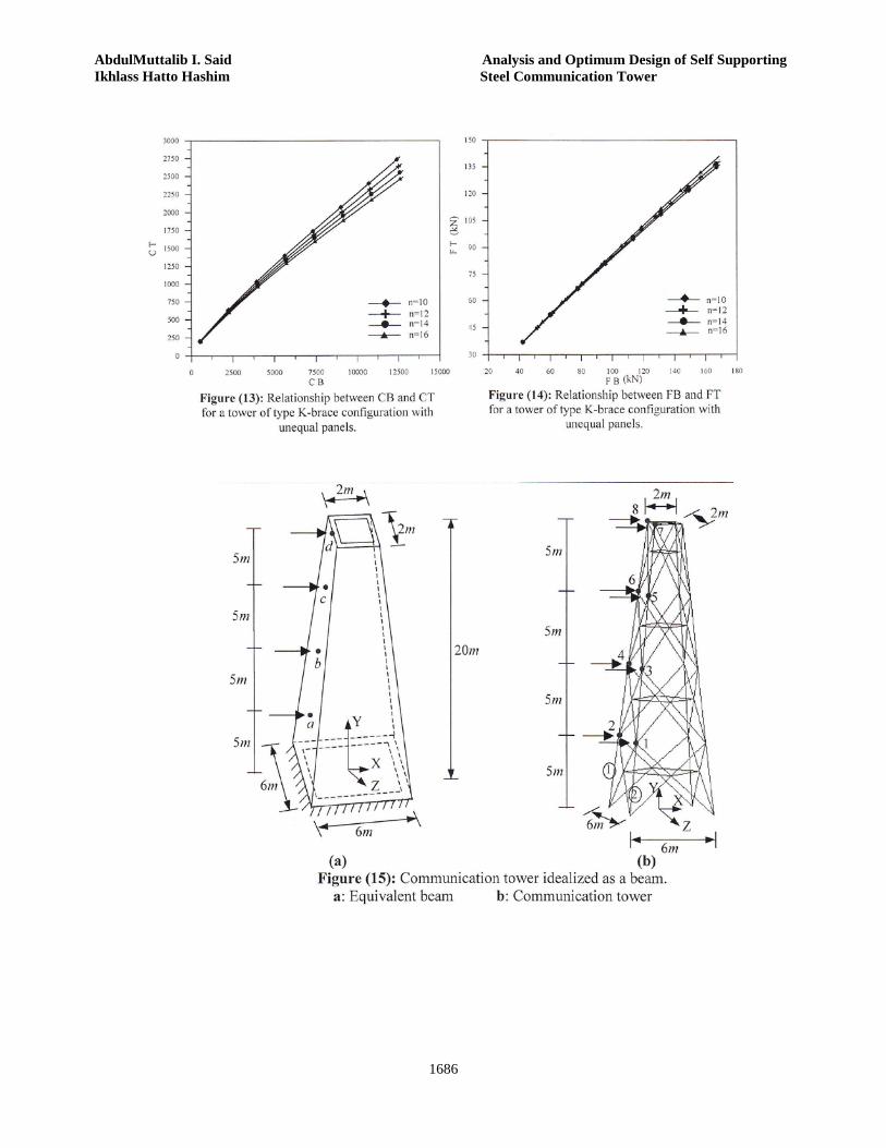
AbdulMuttalib I. Said Analysis and Optimum Design of Self Supporting Ikhlass Hatto Hashim Steel Communication Tower
1686

Journal of Engineering Volume 19 December 2013 Number 12
1687