theoretical concepts and simulations

Theoretical Concepts and Simulations

S. DenisovMNTF, Uni Augsburg

1 / 18

Some words about the course

The lecturer

Sergey Denisov, Theor. Phys. I Dept, MNTF, Uni AugsburgCan be reached by email:[email protected] office is located in the Institute for Physics, North Building,fifth floor, Theor. Phys. I, room 517.Personal web page:http://www.physik.uni-augsburg.de/~denisose/

The course

Lectures: two times a week (Wednesday, 15 : 45− 17 : 15, &Friday, 14 : 00− 15 : 30), audience T-1005Project: we will discuss the procedure next week

2 / 18

mailto:[email protected]

http://www.physik.uni-augsburg.de/~denisose/


Suggested textbooks

I H. Gould, J. Tobochnik and W. Christian, Introduction toComputer Simulation Methods (3rd ed., Addison Wesley,Reading MA, 2006) (Java).

I W. Kinzel and G. Reents, Physik per Computer(Physikalischer Probleme mit Mathematica und C )

I P. DeVries and J. Hasbun, A First Course in ComputationalPhysics (2nd ed., Jones & Bartlett Publishers, 2010) (Matlab)

3 / 18


Suggested on-line courses (reference material)

I R. Fitzpatrick, Computational Physics: An introductorycourse (C and C + +),http://farside.ph.utexas.edu/teaching/329/lectures/lectures.html

I Computational Physics using MATLAB, http://www.physics.

purdue.edu/~hisao/book/www/Computational_Physics_using_MATLAB.pdf

I Computational Physics with Python,http://www-personal.umich.edu/~mejn/computational-physics/

http://phys.csuchico.edu/ayars/312/Handouts/comp-phys-python.pdf

4 / 18

http://farside.ph.utexas.edu/teaching/329/lectures/lectures.html

http://www.physics.purdue.edu/~hisao/book/www/Computational_Physics_using_MATLAB.pdf

http://www.physics.purdue.edu/~hisao/book/www/Computational_Physics_using_MATLAB.pdf

http://www-personal.umich.edu/~mejn/computational-physics/

http://phys.csuchico.edu/ayars/312/Handouts/comp-phys-python.pdf


Topics

I basic things: numerical precision and accuracy of simulations,random number generation, interpolation, differentiation,integration, roots of an equation, extremes of a function;

I ordinary differential equations (ODEs): Euler method,predictor-corrector methods, Runge-Kutta method, somespecific integrators;

I basic matrix operations, linear equations systems, eigenvalueproblems and matrix decompositions;

I Fourier analysis, discrete and fast Fourier transform, Fouriertransform in higher dimensions;

I Partial differential equations, initial value problems, boundaryvalue problems;

5 / 18


Topics (continuation)

I molecular dynamics simulations, percolation, diffusion limitedaggregation and ab-initio molecular dynamics

I ordinary differential equations (ODEs): Euler method,predictor-corrector methods, Runge-Kutta method, somespecific integrators;

I Monte-Carlo simulations, sampling and integration,Metropolis algorithm;

I simulations of open quantum systems: Monte Carlowave-function method (also called ’quantum-jump approach’).

6 / 18

Computational physics

Goals

I calculate solutions to physics problemsI Take advantage of the fact that all physics problems are

(should be) formulated mathematicallyI Solve equations!

I display solutions in a way that helps you (us, them) interpretand understand the underlying physics

7 / 18


Formulate the problem & then solve the equations

I There are many different types of equations:I algebraic (polynomial)

I trigonometric, logarithmic

I differential, integral

I linear, nonlinear

I you may have a single equation to solve or a set of equationsthat must be solved simultaneously

I your need to propagate the equation(s) which may depend oninitial or boundary conditions

8 / 18


See the results

I In most cases, you need to make a plot of the solution, inorder to visualize how certain quantities depend on others.

I xmgrace (simple graphs)

I gnuplot (good for almost everything)

I matlab (very convenient)

I Origin (the best, but very expensive)

I how to visualize the results is an issue itself

9 / 18


The computer does what it was told to do

I The work in solving a problem is still to be done

I derive the equations that represent the system of interestI understand all the approximations and limitations (conditions

for validity)I determine how to instruct the computer to solve the equationsI undestand all shortcoming and pitfalls of computer simulations

I results of simulations ⇔ theoretical predictions

I comparison with measurements

10 / 18


Tools and means

I programs such as Mathematica and MATLAB can help youwork with equations analytically

I symbolic manipulationI might help you obtain analytical solution

I in most cases the equations have to be solved numerically

I smooth functions must be discretizedI derivatives become differencesI integrals become sumsI errors (round-offs, approximation, ect) must be carefully

tracked

11 / 18

Computer number representations and numericalprecision

An example

Having only floating numbers with 5 decimal digits, we wish toevaluate the function

f (x) =1− cos(x)

sin(x)

for some small value of x . By multiplying the denominator andnumerator with 1 + cos(x) we get

f (x) =sin(x)

1 + cos(x)

Take x = 0.007 (in radians). For the chosen precision we get

sin(0.007) ≈ 0.69999× 10−2, cos(0.007) ≈ 0.99998

12 / 18


An example (continuation)

First expression for f (x) results in

f (x) =1− 0.99998

0.69999× 10−2=

0.2× 10−4

0.69999× 10−2= 0.28572× 10−2

while the second expression results in

f (x) =0.69999× 10−2

1 + 0.99998=

0.69999× 10−2

1.99998= 0.35000× 10−2.

The former results is wrong, the latter is the exact. For x ≈ π thesituation is reversed.Not, that if had chosen a precision of 6 leading digits, bothexpressions yield the same answer.

13 / 18


IEEE fixed-point numbers

Fixed-point numbers, i. e. numbers with fixed number of digitsbeyond the decimal point are rare in computational physics(integers mostly, combinatoric problems etc). A fixed-pointrepresentation with N bits looks

,

where n + m = N − 2.Their range (for N = 32) is −2147483648 ≤ x ≤ 2147483647An advantage of this representation is that all numbers have thesame absolute error 2−m−1. The biggest disadvantage is thatsmall numbers have large relative errors. In real-world applicationswe are concerned about relative errors more than about absoluteones. 14 / 18


IEEE floating-point numbers

Floating-point numbers are stored as a concatenation of (1) thesign bit s, (2), the exponent e, and (3) the mantissa f ,

Singles: 32 bits for all; Doubles: 32 + 32 bits for allA single: s: a single bit, e: 8 bits (0 ≤ e ≤ 255), f : 23A double: s: a single bit, e: 11 bits (0 ≤ e ≤ 2047), f : 52 bitsThe stored exponent e is always positive, and a fixed umber bias isadded to the actual exponent before it is stored as the biasedexponent e. The actual exponent is

p = e − bias

Singles: bias = 127, doubles: bias = 102315 / 18


IEEE floating-point numbers (continuation)

The IEEE standard for primitive data types

Serious scientific calculations always require double-precision floats!16 / 18


Machine precision (an example)

Consider the addition of two single-precision numbers

7 + 1.0× 10−7 =?

Both numbers are stored as bit sequences

17 / 18


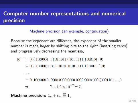
Machine precision (an example, continuation)

Because the exponent are different, the exponent of the smallernumber is made larger by shifting bits to the right (inserting zeros)and progressively decreasing the mantissa,

Machine precision: 1c + εmdef= 1c

18 / 18

theoretical concepts and simulations

Documents