EUROPEAN ORGANIZATION FOR NUCLEAR RESEARCH ORGANISATION EUROPEENNE POUR LA RECHERCHE NUCLEAIRE

CERN - PS DIVISION

PS/ BD/ Note 97-06 /Rev. 1

THEORETICAL AND EXPERIMENTAL INVESTIGATION OF

MAGNETIC MATERIALS FOR DC BEAM CURRENT

TRANSFORMERS

P. Kottman

Abstract

Toroidal cores made of high-permeability magnetic materials are fundamental building blocks of DC beam current transformers (DCBT). The impact of the properties of the magnetic cores on the overall performance of DCBT was studied. The principle of the DCBT operation is based on the superposition of AC and DC electromagnetic fields in the cores. This effect was studied in detail in two magnetic materials currently used in a construction of DCBT at CERN. The simulation of the DCBT operation was made using the results of these studies and the theoretical model for description of a B-H hysteresis curve of magnetic materials. This simulation allows to evaluate the influence of various factors (a shape of the B-H curve, deviations of core parameters, presence of noise) on the performance of DCBT. A survey of available high-permeability magnetic materials suitable for DCBT is presented.

Geneva, Switzerland 21January1998

1. Introduction.

DC Beam Current Transformers (DCBT) are well established beam diagnostic

instruments [Borer & Jung 1984, Koziol 1989, Gelato 1992 ]. At CERN their use was

required for the first time in ISR machine [Unser 1969 ] where the beam was kept

circulating for long periods of time and therefore traditional AC transformer techniques

involving the integration of the beam current (charge) were impossible to use. Later

the need to measure a DC component of a beam current lead to the use of DCBT

monitors also in the PS machine and Antiproton project [ Unser 1981, Koziol 1995 ],

as well as in LEP and SPS [ Unser 1989, Vos 1994 ]. In the future, DCBT monitors

will play their role in beam instrumentation for LHC, too [Andersson 1994, Vos 1994].

Requirements of various machines in terms of the DC current resolution were

surnmarised in [ Odier & Maccarini 1997 ]. It was shown that in majority of cases the

resolution of presently available DCBT monitors (in the range of µA) is sufficient

because the intensity of the beam current is well above it. However, there are a few

cases where the beam current is comparable or even lower than the resolution of

DCBT. These are the cases where either a number of particles is very low (e.g. pbar),

or the velocity is very low (e.g. deceleration projects), or the circumference of the

machine is large (e.g. LHC). Therefore there is a need for finding ways how to

improve the performance of DCBT monitors.

DCBT monitors consist of two main parts: an assembly of toroidal magnetic

cores and electronics circuitry. The present state and possible further improvements of

the electronics of DCBT have been described elsewhere [ Odier & Maccarini 1997,

Unser 1991 ]. It is obvious that it is desirable to have the noise level in the electronics

as low as possible to improve the resolution of DCBT. On the other hand, the role of

the magnetic cores in the overall performance of DCBT was not clearly established

before. In fact, two quite different opinions on this subject could be found in the

literature. According to the first one [ Unser (1993)] " ... the resolution, zero stability

and temperature drift of the DCBT depend on the quality of the modulator core pair

and the resolution is only limited by magnetic modulator noise (Barkhausen) ... ". The

second opinion [ Vos (1994)] is that" ... magnetic noise (Barkhausen) generated in the

tori can be neglected; . . . there is no sign of a requirement concerning the magnetic

properties of the rings;... nevertheless, the magnetic properties of the tori are

important...". With the situation like this there was an obvious need to find out more

exactly the extent to which magnetic cores can determine the performance of DCBT.

Therefore the aim of this project was to investigate the influence of various factors,

such as a shape of a B-H hysteresis curve of a magnetic material, possible differences

between the cores of DCBT ('matching error') or presence of Barkhausen noise in

cores on the performance of DCBT, as compared to the influence of factors external to

the cores, such as a noise in a modulator circuit. In order to achieve this aim a program

simulating the operation of DCBT has been made. The program uses a mathematical

model for description of a B-H hysteresis curve of magnetic materials allowing to

generate hysteresis curves which are very similar to the ones found in existing

materials. Another aim of this study was to make a survey of available high­

permeability magnetic materials suitable for DCBT.

2

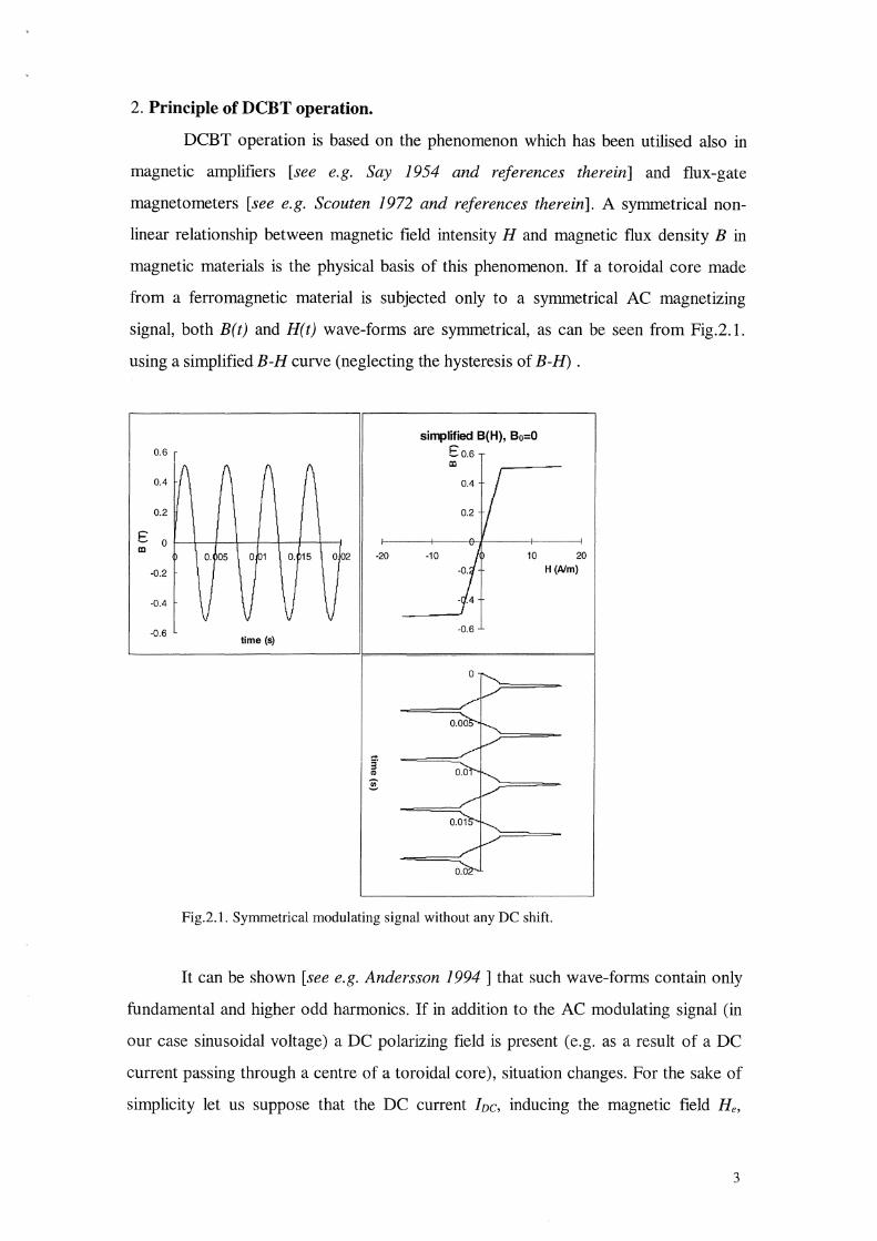
2. Principle of DCBT operation.

DCBT operation is based on the phenomenon which has been utilised also in

magnetic amplifiers [see e.g. Say 1954 and references therein] and flux-gate

magnetometers [see e.g. Scouten 1972 and references therein]. A symmetrical non­

linear relationship between magnetic field intensity H and magnetic flux density B in

magnetic materials is the physical basis of this phenomenon. If a toroidal core made

from a ferromagnetic material is subjected only to a symmetrical AC magnetizing

signal, both B(t) and H(t) wave-forms are symmetrical, as can be seen from Fig.2.1.

using a simplified B-H curve (neglecting the hysteresis of B-H) .

simplified B(H), Bo=O o.6 I ~o.sT

0.4

0.2

E o '"--+---l--+----+--+---1-<---l ID

0. 15 0 02 -20 -10 10 20

-0.2 H (Alm)

-0.4

·0.6 time (s)

-0.6

Fig.2.1. Symmetrical modulating signal without any DC shift.

It can be shown [see e.g. Andersson 1994] that such wave-forms contain only

fundamental and higher odd harmonics. If in addition to the AC modulating signal (in

our case sinusoidal voltage) a DC polarizing field is present (e.g. as a result of a DC

current passing through a centre of a toroidal core), situation changes. For the sake of

simplicity let us suppose that the DC current !De, inducing the magnetic field He,

3

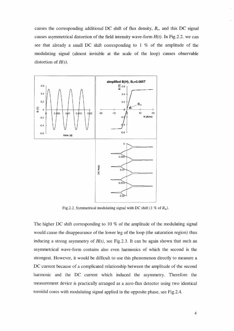
causes the corresponding additional DC shift of flux density, Be, and this DC signal

causes asymmetrical distortion of the field intensity wave-form H(t). In Fig.2.2. we can

see that already a small DC shift corresponding to 1 % of the amplitude of the

modulating signal (almost invisible at the scale of the loop) causes observable

distortion of H(t).

0.6

0.4

0.2

E 0 Ill

0. 05

-0.2

-04 t v -0.6

0 1 0. 15 0 02 -20

v v v time (s)

simplified B(H), Bo=O.OOST Eo.6 Ill

0.4

0.2

~ -0.6 I

~Bo

10 20

H(A/m)

Fig.2.2. Symmetrical modulating signal with DC shift (I % of Bm)·

The higher DC shift corresponding to l 0 % of the amplitude of the modulating signal

would cause the disappearance of the lower leg of the loop (the saturation region) thus

inducing a strong asymmetry of H(t), see Fig.2.3. It can be again shown that such an

asymmetrical wave-form contains also even harmonics of which the second is the

strongest. However, it would be difficult to use this phenomenon directly to measure a

DC current because of a complicated relationship between the amplitude of the second

harmonic and the DC current which induced the asymmetry. Therefore the

measurement device is practically arranged as a zero-flux detector using two identical

toroidal cores with modulating signal applied in the opposite phase, see Fig.2.4.

4

0.6

0.4

0.2

E: 0 t--->--+-+--+--+->-----+--< m

0. 05 001 o. 15 002

·0.2

·0.4

·0.6 time (s)

·20

simplified B(H), Bo=0.05T I=' ;; 0.6

40 60 H (Alm)

·0.6

0

Fig.2.3. Symmetrical modulating signal with DC shift (10 % of Bm).

R

Fig.2.4. Practical arrangement of zero-flux detector.

Vz Synchronous

detector

5

A detailed description of DCBT operation is given in [ Gelato 1992] and description of

DCBT electronics in [Odier & Maccarini 1997].

If we want to simulate the operation of DCBT by a computer program we need

to use some appropriate model for description of the B-H relation of a magnetic

material of the cores. Such a model must inevitably include the hysteresis of B-H which

is always present in real magnetic materials. The model used in our study will be

described in detail in Chapter 4. On the other hand, if we are to simulate the operation

of a real DCBT, we are faced with another problem when we proceed from the

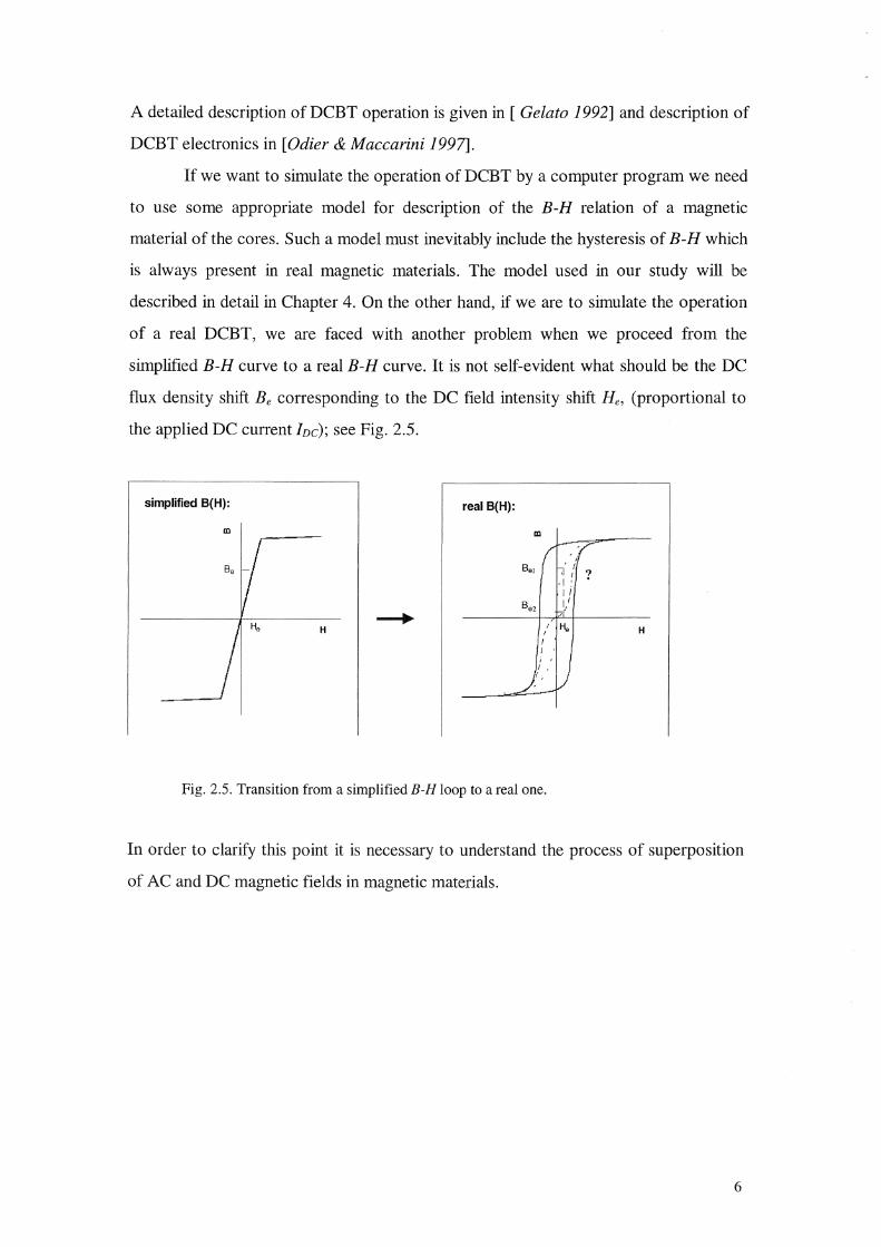
simplified B-H curve to a real B-H curve. It is not self-evident what should be the DC

flux density shift Be corresponding to the DC field intensity shift He, (proportional to

the applied DC current !De); see Fig. 2.5.

simplified B(H): real B(H):

al al

H H

Fig. 2.5. Transition from a simplified B-H loop to a real one.

In order to clarify this point it is necessary to understand the process of superposition

of AC and DC magnetic fields in magnetic materials.

6

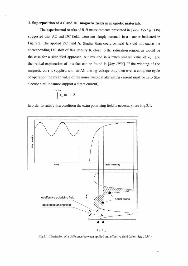
3. Superposition of AC and DC magnetic fields in magnetic materials.

The experimental results of B-H measurements presented in [Boll 1991 p. 330]

suggested that AC and DC fields were not simply summed in a manner indicated in

Fig. 2.2. The applied DC field Ha (higher than coercive field He) did not cause the

corresponding DC shift of flux density Be close to the saturation region, as would be

the case for a simplified approach, but resulted in a much smaller value of Be. The

theoretical explanation of this fact can be found in [Say 1954]. If the winding of the

magnetic core is supplied with an AC driving voltage only then over a complete cycle

of operation the mean value of the non-sinusoidal alternating current must be zero (the

electric circuit cannot support a direct current):

2n/m

I iL dt = 0 0

In order to satisfy this condition the extra polarising field is necessary, see Fig.3.1.

.?;­'iii c GI 'Cl >< :I ;;::

···-···-·····-·-·--···-··--·--···--··-··-·-·-----····----·-········--·····-·1 7'"'"'>:--~~-r-r--r~~~~~-=:======~,-

time field intensity

net effective polarising field §" CD equal areas

applied polarising field

tt Fig.3.1. Illustration of a difference between applied and effective field (after [Say 1954]).

7

As a result of this effect the net effective polarising field, He, is smaller than the applied

polarising field Ha (proportional to foe).

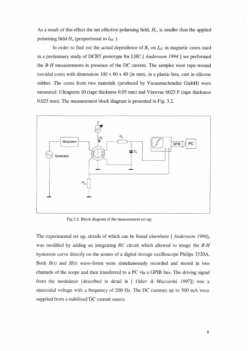
In order to find out the actual dependence of Be on foe in magnetic cores used

in a preliminary study of DCBT prototype for LHC [Andersson 1994] we performed

the B-H measurements in presence of the DC current. The samples were tape-wound

toroidal cores with dimensions 100 x 80 x 40 (in mm), in a plastic box, cast in silicone

rubber. The cores from two materials (produced by Vacuumschmelze GmbH) were

measured: Ultraperm 10 (tape thickness 0.05 mm) and Vitrovac 6025 F (tape thickness

0.025 mm). The measurement block diagram is presented in Fig. 3.2.

GPIB

1 1

Fig.3.2. Block diagram of the measurement set-up.

The experimental set up, details of which can be found elsewhere [Andersson 1994],

was modified by adding an integrating RC circuit which allowed to image the B-H

hysteresis curve directly on the screen of a digital storage oscilloscope Philips 3320A.

Both B(t) and H(t) wave-forms were simultaneously recorded and stored in two

channels of the scope and then transferred to a PC via a GPIB bus. The driving signal

from the modulator (described in detail in [ Odier & Maccarini 1997]) was a

sinusoidal voltage with a frequency of 200 Hz. The DC currents up to 500 mA were

supplied from a stabilised DC current source.

8

The results of the experiments are presented in Fig. 3.3 for Ultraperm 10 and

Fig.3.4. for Vitrovac 6025 F, respectively.

0.8 ~ OmA I . .n".---

--500 mA I//" 0·6 ~ --shift 1---+---t--J-Y---l-t---+---+---+---+--.

0.4 l---+---+---+---1---+-t-+--l--___,I--___, _ ___, _ __,

0.2

E 0 ID

-0.2

-0.4

-50 -40 -30 -20 -10 0 10 20 30 40 50

H(A/m)

Fig.3.3. Dependence of Be on Ive in Ultraperm 10.

0.6

0.4

--OmA ,r ----···-·- 200 mA c---- v ----500mA

--shift

0.2

I i=' 0 ar

I

-0.2

-0.4 ' J -0.6 •->"~ ••••

-30 -20 -10 0 10 20 30

H(Nm)

Fig.3.4. Dependence of Be on Ive in Vitrovac 6025 F.

9

We can see that in accordance with the above presented theory the shift of flux density,

Be, for a given applied Ive (and corresponding Ha) is much smaller than would be the

case if a pair of values Be and Ha were directly taken form the simplified B-H curve.

This result has two important consequences on the operation of DCBT. The first is

positive and concerns the upper range of currents: for a given cores even relatively

high currents ( - amperes) will not cause Be to approach the value of saturation flux

density, Bs, and therefore there is no danger that B(t) would remain always in the

saturation region causing disappearance of the second harmonic in the H(t) signal. The

second consequence is negative and concerns the lower range of currents: very low

DC currents (- microamperes) will result in very low values of Be and therefore in very

small induced asymmetry in the H(t) signal (and the correspondingly small second

harmonic amplitude).

10

4. A mathematical description of the B-H hysteresis loop.

There exists a large amount of models describing the B-H relation in magnetic

materials. Some of them derive the shape of the macroscopically observed hysteresis

loop from a complex behaviour of individual magnetic moments or domains [ see e.g.

Philips 1994 and references therein ]. Such models are inevitably quite complicated to

work with and computation of hysteresis loops is very time consuming. In many cases

(when a magnetic material is used in a given application) it is not necessary to know

the exact nature of changes of magnetic properties at the level of individual magnetic

moments and it is sufficient to use more simple models for a B-H loop [see e.g. Rivas

1981 and references therein ]. We have found out that for a simulation of behaviour of

a DC beam current transformer (DCBCT) the analytical hysteresis model proposed in

[ Cortial 1997] is very suitable because in spite of its relative simplicity it provides a

good degree of accuracy and flexibility in generating the B-H loops of various shapes.

The main parameters of the model are: the coercive field He, the slope of the

loop at He, k; the field intensity H1 , the flux density B1 and the slope of the loop f) at

the point corresponding to the end of the irreversible part of the B-H curve, and the

saturation field intensity H.1· and flux density B.1., see Fig.4.1.

- ~e ...

·k=dB/dH /.

Fig.4.1. Definition of the parameters of the model.

11

The original model of Cortial et al. was given in terms of relation between the field

intensity, H, and magnetization, M, instead of flux density, B. In our application it is

more convenient to work with the flux density, B, therefore the original model was

changed accordingly. The model was also slightly modified to enhance its flexibility;

the modifications will be described below. In the model the irreversible part of the B-H

curve, i.e. in the interval (-Hh H1) , and the reversible part, i.e. IHl>Hf, are described by

two different formulae. The relation between B and H is expressed in terms of the

normalized field intensity h and flux density b defined by h=H!Hf and b=B!Bf.

The irreversible part of the B-H curve is expressed using the parameters Q, R

and the function g defined by the following relations:

Q=Hc/Ht

R=-kQH1 (l-Q) 2 /B1

(h)= 1-(h/Q) g (l-h2)

(4.1)

(4.2)

(4.3).

The b-h relation is then given by the sum of an hyperbolic tangent and an arctangent

functions, which results in a well-known shape of the hysteresis loop. The additional

linear function influences the slope of the loop at the closure point h= 1:

b(h) = {K1 tanh[R g(h)]+ (K2 In) arctan[(n I 2) R g(h)]}(l- tan 8) + h (tan 8) (4.4).

In the original model as given in [ Cortial 1997] the parameters K1 and K2 were not

introduced and were given as the exact values K1=0.5 and K2=1, respectively.

However, we have found out that introducing these parameters gives more flexibility in

describing mathematically the loops generally found in the common magnetic materials.

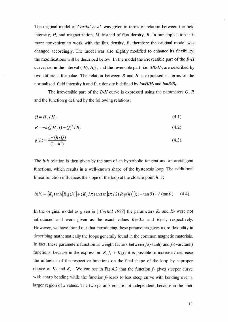
In fact, these parameters function as weight factors between f 1( -tanh) and f2(-arctanh)

functions, because in the expression K1 f 1 + K2f2 it is possible to increase I decrease

the influence of the respective functions on the final shape of the loop by a proper

choice of K1 and K1. We can see in Fig.4.2 that the function f 1 gives steeper curve

with sharp bending while the function f2 leads to less steep curve with bending over a

larger region of x values. The two parameters are not independent, because in the limit

12

h--* 1 we have f1--* 1 andfi --* 0.5 and K1 f1 + Kzfi = 1, therefore K2 = 2 (1- K1 ). In

order to satisfy the validity of Eq. ( 4) in the limit h --* 1, i.e. b --* 1, we added after the

first part of Eq. ( 4) the term (1-tan B ), which was not present in the original model.

0.8

0.6

>-0.4

0.2

0 10

--tanh(x)

--(1/pi)*atan[(pi/2)x]

20

x 30 40

Fig.4.2. The functions used for a description of the irreversible part of the loop.

We have also found that the shape of the loop near the closure point H=H1 can be

influenced by changing the power in the expression (2) and therefore we replaced the

exact value of 2 by an adjustable parameter K3 .

The reversible part of the B-H curve (Hr < H < H_,. ) is described by the

parabolic function:

B (H)=A1 H2 + A1 H + A3 (4.5)

where the parameters A1 , A1 and A3 are calculated from the border conditions:

=tanB dH H1

dB =0 dH Hs

(4.6)

(4.7)

(4.8).

In the original model, using the magnetization M , the condition (8) corresponded to a

well known fact that after the saturation the magnetization remains constant, equal to

M., . . In our modification, using B, the flux density continues to increase after the

complete saturation, because B = µo H for H > Hs . In order to respect this condition

13

in generating the B-H curve we used the field intensity Hm < H.,. , allowing to retain a

non-zero slope of the B-H curve at the extreme points.

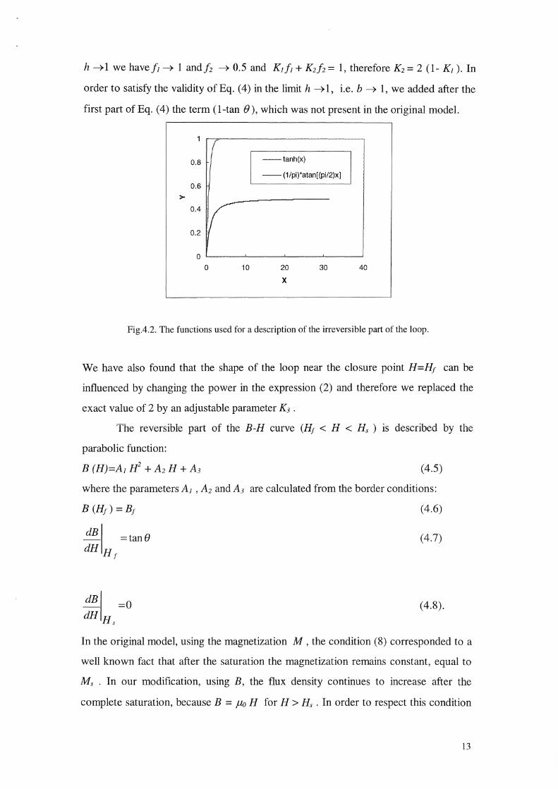
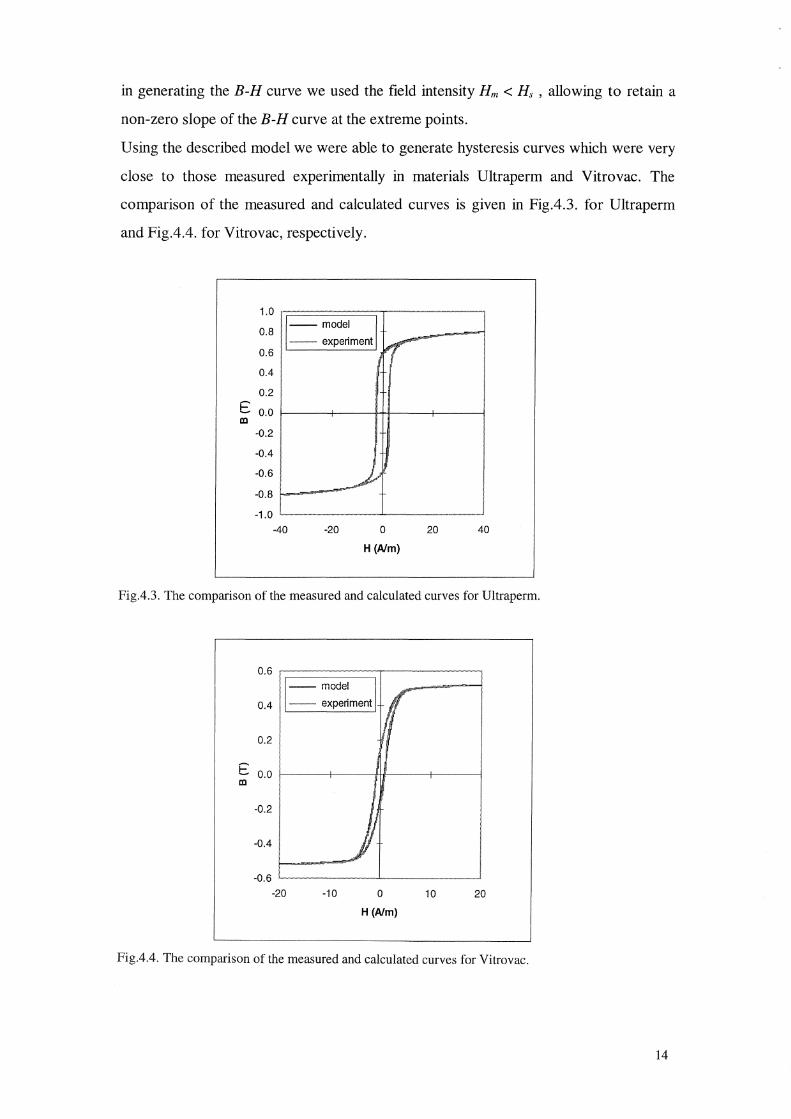
Using the described model we were able to generate hysteresis curves which were very

close to those measured experimentally in materials Ultraperm and Vitrovac. The

comparison of the measured and calculated curves is given in Fig.4.3. for Ultraperm

and Fig.4.4. for Vitrovac, respectively.

1.0

0.8 -- model

-- experiment 0.6

0.4

0.2

E 0.0 aJ

-0.2 I -0.4

-0.6

-0.8

-1.0 ~-~-.~

-40 -20 0 20 40

H (Alm)

Fig.4.3. The comparison of the measured and calculated curves for Ultraperm.

E

0.6 ~-·

Ill_ model

0.4 -- experiment

I I 0.2 I

0.0 1-----1----+li----+----l

-0.2 I

:: '"-··~--~~-J -20 -10 0 10 20

H (Alm)

Fig.4.4. The comparison of the measured and calculated curves for Vitrovac.

14

5. Simulation of the operation of a DC beam current transformer (DCBCT):

programme.

In order to study the influence of various parameters, such as a shape of a B-H

loop, magnitude of the modulation signal, differences between two magnetic cores of a

DCBCT or various kinds of noise, a simulation of the operation of the DCBCT was

made. The software package MATLAB was used for this simulation, due to its

powerful features e.g. in a polynomial approximation of curves, calculation of special

functions and FFT analysis of signals. The results of the simulation are:

- the wave-forms of the signals B(t) and H(t) in the two cores of the DCBCT and the

signal dH(t)=HJ(t)+H2(t) ; optionally can be saved as an ASCII-file

- the power spectrum of dH(t) and specially the 1st and the 2nct harmonic amplitude as a

function of a DC current - optionally can be saved as an ASCII-file.

In the process of the simulation the model introduced in Chapter 4 was used for

a description of the B-H curve of the magnetic material of the cores. However, the

model describes the flux density B as a function of the field intensity H. During the

operation of the DCB CT we generate a modulating signal which produces a sinusoidal

changes of the flux density B and therefore we need to know how the field intensity H

changes as a function of B. In saturation regions of the B-H curve this fact poses no

problems because we simply find the inverse function to the parabolic function (4.8). In

the irreversible part we used the following procedure: in the first step we generated the

B(H) curve using the defined set of parameters, then having a set of corresponding B

and H values we made a polynomial approximation of H as a function of B. The

calculated polynomial coefficients were then used in the process of the simulation of

theDCBCT.

The simulation program consists of the following parts:

1. definition of parameters of the model for a description of the B-H loop in the core

No. I and possible differences in the core No.2; there are 3 default sets of parameters:

for the B-H loop of a general shape and for the loops corresponding to the Ultraperm

10 and Vitrovac 6025F materials, respectively.

2. generation of the B-H loop and finding the polynomial approximation for H(B) in

the cores No.1 and No.2, respectively.

15

3. adding a noise with a possibility to add several components of noise of various

kinds: sinusoidal (e.g. 50 Hz), random, Barkhausen-type noise; the amplitude of the

noise can be defined as a percentage of the amplitude of the modulation signal Bm.

4. input for a DC current with a possibility to define the interval< IDcmin, locmax >.

5. calculation of the shift Bo corresponding to the shift Ho - foe.

6. generation of the modulation signal (including the noise).

7. calculation of the signals HJ(t), H 2(t) and dH(t) with a graphical output on the

screen.

8. the FFT analysis of the dH(t) signal.

The results of the MATLAB command 'fft(y)', where y is the function to be subjected

to the FFf spectral analysis (y is defined by a set of N discrete points), are given as a

complex Fourier coefficients, from which the amplitude (magnitude) of the respective

spectral components can be obtained by calculating the sum of squares of the real and

imaginary parts of coefficients. The results obtained by this procedure depend on the

number of discrete samples N and therefore it makes no sense to try to interpret the

amplitude in terms of real physical units. The arbitrary units will be used when

presenting the influence of the shape of the B-H curve on the 2nd harmonic component.

When the influence of presence of noise and differences between the cores is studied,

the results will be presented as the ratio between the FFf amplitude of spectral

components of the dH(t) signal and the FFf amplitude of the fundamental frequency of

the modulating signal.

16

6. Simulation of the operation of a DC beam current transformer (DCBCT):

results.

6.1. The influence of a loop shape.

The possible influence of a shape of the B-H curve on the overall performance of

DCBT was studied by generating various loops and comparing the 2nct harmonic

amplitude obtained as a result of a simulation programme described in Chapter 5. For

this purpose a kind of a 'catalogue' of B-H loops was made using a default set of loop

parameters as a starting point and then gradually changing the parameters to generate

loops of various shapes. The sets of parameters are presented in Tab.6.1. (bold

numbers indicate a different parameter as compared to the default set).

Loop No. 1 2 3 4 5 6 7 8 Parameter Hm(A/m) ')(\ 30 30 30 30 30 30 30 vv

Hc(A/rn) 1.8 1.8 1.8 1.8 1.8 0.5 0.5 0.5 Hf(A/rn) 7 7 7 7 7 7 7 7 Hs(A/rn) 40 40 40 40 40 40 40 40 Bf(T) 2 2 2 2 2 2 2 2 Bk(T) 0.7 0.7 0.7 0.7 0.7 0.7 0.7 0.7 k 10 10 10 5 50 10 50 10

e 0.03 0.01 0.005 0.005 0.005 0.005 0.005 0.005

K1 0 0 0 0.5 0 0 0 0.5 K2 6 6 2 2 2 6 2 2

Tab.6.1. The parameter sets for various B-H loop shapes.

The corresponding loops are presented in Fig.6.1.

_,,,,..,,,..,,_~,,,_,,.,,,,

0.8

0.6

0.4

0.2

I

------I

vr I j

0.8

0.6

0.4

0.2

E 0 E 0 ID ID

-0.2

-0.4

-0.6

-0.8

-1

j J

) ,I --~ ' ---~,,~-~-~ -~···~-- ~-_J

-0.2

-0.4

-0.6

-0.8

-1

-20 -10 0 10 20 -20

H (Alm)

Loop no.I.

-10

.-7'

/{ I

J

) /

~

0

H(Am)

l I

-~-~~~~

10 20

Loop no.2.

17

0.8

0.6 I

0.4

0.2

E 0 aJ

-0.2

-0.4

-0. 6 f-----+--_./-1--V-------if----I

-0.8 f-----+---+----+------l

-1 L_ __ ,. ______ " -~"-•·---'------"--·---"'

-20 -10 0 10 20

H (Alm)

Loop no.3.

0.8

0.6

0.4

0.2

E 0 aJ

-0.2

-0.4 I -0.6

-0.8 lf-----+---+-----+------l

-1 L-....... ,.,..,. ... ··-·-"- ~-,.--~ ~---"~" __ J -20 -10 0 10 20

H (Alm)

Loop no.5.

0.8

.········.··.·· -

I 0.6

0.4

I I ' I

0.2 I

E 0 aJ

-0.2

-0.4

-0.6

-0.8 I -1 ,_~..._, ____

-20 -10 0 10 20

H (Alm)

Loop no.7.

Fig.6.1. Various B-H loop shapes.

E aJ

E aJ

E aJ

0.8

0.6

0.4

0.2

0

-0.2

-0.4

-0.6

-0.8

-1

-20

0.8

0.6

0.4

0.2

0

-0.2

-0.4

-0.6

-0.8

-1 ~--

-20

-10

I

0

H(Am)

10

Loop no.4.

20

I _ __._ __ __.__ ____ ~J

-10 0 10 20

H (Alm)

Loop no.6.

1 ,-~-~-

o.8 I 0.6 I

T

0.4

0.2

0

-0.2

I -0.4

-0.6

-0.8 f----t----+----1-------l

-1

-20 -10 0 10 20

H (Alm)

Loop no.8.

18

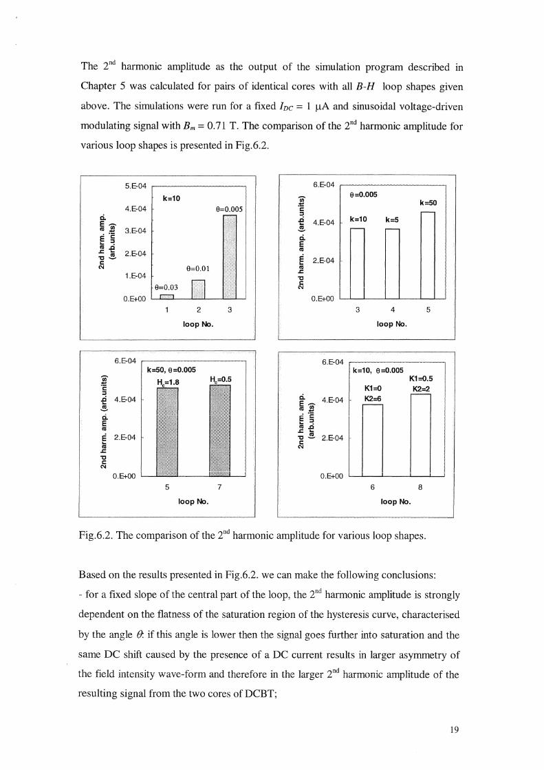
The 2nd harmonic amplitude as the output of the simulation program described in

Chapter 5 was calculated for pairs of identical cores with all B-H loop shapes given

above. The simulations were run for a fixed Ive = 1 µA and sinusoidal voltage-driven

modulating signal with Bm = 0.71 T. The comparison of the 2nd harmonic amplitude for

various loop shapes is presented in Fig.6.2.

5.E-04

k=10 4.E-04

ci. E ....... I'll .l!l 3.E-04 . ·2 E ::i .... I'll ..c .c ... 2.E-04 "C .!!!.. c N

1.E-04

O.E+OO 2

loop No.

6.E-04 k=50, 0=0.005

(ii' .... '2 :I

..ci 4.E-04 ... ~ Q. E Cll

E 2.E-04 ... Cll ..c "C c:

N

I 0=0.0051

3

6.E-04

(ii' ~ c :I

..ci 4.E-04 ... ~ ci. E I'll

E 2.E-04 ... I'll ..c "C c N

O.E+OO

ci. E ....... I'll rn -E 'E ... =! I'll ..c ..c .....

"C ~ c: N

2.E-04

---~----

0=0.005 k=50 ~

k=10 k=5 r-- r--

3 4 5

loop No.

~~~~~~~I l~~-O.E-+00~-6-loo-pNo~·-8~ O.E+OO

5 7

loop No.

Fig.6.2. The comparison of the 2nd harmonic amplitude for various loop shapes.

Based on the results presented in Fig.6.2. we can make the following conclusions:

- for a fixed slope of the central part of the loop, the 2nd harmonic amplitude is strongly

dependent on the flatness of the saturation region of the hysteresis curve, characterised

by the angle (}. if this angle is lower then the signal goes further into saturation and the

same DC shift caused by the presence of a DC current results in larger asymmetry of

the field intensity wave-form and therefore in the larger 2nd harmonic amplitude of the

resulting signal from the two cores of DCBT;

19

- for a fixed value of the angle e, the 2nd harmonic amplitude increases with the

increase of a slope of the central part of the loop characterised by the parameter k

(corresponds to the increase of permeability of the magnetic material);

- for the fixed values of both k and () , the 2nd harmonic amplitude is slightly higher for

a lower value of the coercive field, He , i.e. for a more narrow loop; although this

dependence is not very pronounced, in AC applications it is generally desirable to use

materials with narrow loops in order to decrease hysteresis losses (proportional to the

area of the loop)

- the 2nd harmonic amplitude is slightly dependent also on the minor details of the loop

shape, such as a rounding close to the closure point of the loop - differences in the

rounding are characterised by the different sets of the parameters K1 and K2 with the

fixed values of both k and () .

20

6.2. The influence of differences between the two cores of DCBT (matching

error).

Ideally the two cores of DCBT should be identical (to have an identical B-H loop) and

this identity should be preserved under all conditions (e.g. when temperature is

changed). In reality it is difficult (if not impossible) to find two absolutely identical

cores, because even the cores from the same production batch slightly differ in one or

more parameters. Not all parameters of a magnetic material are equally likely to differ

from one core to another. Parameters such as saturation flux density B.1. , Curie

temperature tc or electrical resistivity p depend only upon the composition of an alloy

(which can be well controlled) and do not change substantially in the process of

manufacturing a component from the alloy. On the other hand, parameters such as

permeabilityµ, coercive field He or remanent flux density B, are drastically affected by

small amounts of certain impurities, heat treatment, residual strain, grain size or plastic

deformation. Therefore the latter group of parameters is much more likely to exhibit

differences from core to core.

In order to evaluate the influence of the matching error on the performance of DCBT

the simulation program enables to introduce a defined difference between the two

cores of DCBT. The simulations were run for a difference in the slope of a loop k at He

(corresponding to differences in permeability), a difference in He and for a difference in

a loop closing point Bk. In the following the results obtained with a loop shape

corresponding to the experimentally measured loop of Ultraperm 10 material are

presented. The results for Vitrovac 6025F were qualitatively practically identical. The

simulations were run for direct current Ive defined in the interval from -100 µA to 100

µA with a step of 1 µA apart from the region from -1 µA to 1 µA where the step of

0.1 µA was used in order to see whether the sub-µA resolution is in principle possible

to achieve with DCBT.

The loops for a default Ultraperm set of parameters (core #1) and for a difference ink

of 1 % and 10% (core #2) are presented in Fig.6.3. The difference of 1 % is practically

invisible and l 0% causes only a small difference in the rounding region of the loop.

However, these differences have serious influence on the harmonics amplitudes as a

function of Ive as can be seen from Fig.6.4. Although the difference of 1 % does not

change 2nct harm - f (Ive) significantly, it leads to appearance of a relatively strong 1st

21

0.8

--core#1 0.6 --core #2, 1 %

------··core #2, 10% 0.4

0.2

E 0 m

-0.2

-0.4

-0.6

-0.8 _ ____J

-20 -10 0 10 20

H (Alm)

Fig.6.3. B-H curves for two cores with different k.

0

-20

-40

iii' '.!:.. Q)

"C -60 ::I :!::! ii E Ill

-80

-100

-120

-0.1 -0.05

---identical cores, 2nd. harm .

.. . . . ,. ... diff. 1 %, 1st harm.

- - - - -diff. 1%, 2nd harm

diff. 10%, 1st harm.

- .. - .. -diff. 10%, 2nd harm.

0 0.05

Ide (mA)

0.1

Fig.6.4. The amplitude of harmonics as a function of Inc for two cores with different k.

22

0.8 ------·--- ·········-·····

--core #1 .~ -·-·

0.6

0.4

0.2

E 0

- --core#2, 1% F/'

! (/ t ·-·-·····core #2, 10%

1/ I

I !

I t

Ill ;

-0.2 l

-0.4

-0.6

I

A ! I

-~ ... tt··-

-0.8

-20 -10 0 10 20

H (Alm)

Fig.6.5. B-H curves for two cores with different He.

0 ,.......-

-20

An - .. u

m ::!:!.. Gl "ti -60 ::l :!::: ii E ro

-80

-100

-120

-0.1 -0.05

---identical cores, 2nd harm.

····-·----dill. 1%, 1st harm.

...... dill. 1 % , 2nd harm.

dill. 10%, 1st harm.

- .. - .. -dill. 10%, 2nd harm

0 0.05

Ide (mA)

0.1

Fig.6.6. The amplitude of harmonics as a function of foe for two cores with different

23

0.8

0.6 --core #1 ,__ __ ,,______,. __ -r-----j

--·-- core #2

0.4

0.2

E ID

-0.2

-20 -10 0 10 20

H (Alm)

Fig.6.7. B-H curves for two cores with different Bk··

0

-20 I

-40

m ~ Q)

"CJ -60 :::J ;!:!

i5. E "' -80

-100

-120

-0.1 -0.05

---identical cores, 2nd harm. -----dill. 0.1%, 1st harm. ......... dill. 0.1%, 2nd harm.

dill. 1%, 1st harm. -··----dill. 1%, 2nd harm. ......... dill. 1% Bk+Bm, 2nd harm.

: :

0 0.05 0.1

Ide (mA)

Fig.6.8. The amplitude of harmonics as a function of foe for two cores with different

Bk.

24

harm. component of dH signal (in the identical cores 1st harm. is well below -120 dB

level). The difference of 10 % causes a flattening of 2nd harm - f Uvc) (i.e. worse

resolution of the system) as well as observable offset. Also the 1st harmonic further

increases. Similar behaviour can be observed also in the case when the cores differ in

the value of a coercive field He , see Fig.6.5 and Fig.6.6.

The situation with different loop closing point Bk is presented in Fig. 6.7. and 6.8. We

can see that harmonics amplitudes are extremely sensitive even to the slightest

deviations in this region - for example the difference in Bk of only 0.1 % has an effect

on 2nd harm - f (Ive) comparable to that of the difference of 10% in He. On the other

hand, if we slightly adjust the amplitude of the modulation signal in the core #2 it is

possible to restore almost completely the resolution of the pair. In fact, such an

adjustment has been successfully used in practical DCBT systems [Gelato 1992 ].

25

6.3. The influence of noise.

In DCBT systems various types of noise may be present. In our simulation program we

examined the influence of sinusoidal line frequency noise, random noise and

Barkhausen-like noise. The last type is a noise specific to magnetic materials and is

caused by discontinuities of the magnetization processes in the steep part of the B-H

loop (irreversible domain displacements= Barkhausen jumps). In the saturation region

a dominant magnetization process is a rotation of magnetization vectors in domains

and such a continuous process does not contribute to noise. Therefore in the

simulation program Barkhausen noise is modelled simply as random noise with

amplitude modulation such that the maximum amplitude occurs close to the coercive

field He and then the amplitude decreases to zero in the saturation region. Barkhausen

noise of this character was experimentally observed [Swartzendruber 1990 ]. (Note:

Barkausen jumps were observed also in saturation region [Scouten 1970 ] but the

amplitude of the corresponding noise was of the order of nT, therefore many orders of

magnitude lower than the modulating flux density - in the following it will be shown

that much higher levels of noise of this type do not have a strong influence on the

DCBT operation).

In order not to mix various influences on performance of DCBT a pair of identical

cores was used in the simulation studies of noise influence.

Sinusoidal line frequency noise even with relatively high amplitude equal to 0.1 % Bm

does not cause serious degradation of DCBT performance, as can be seen in Fig.6.9.

Dependence 2nd harm - f (Ive) is very close to that in absence of noise. Situation is

similar with a sinusoidal noise of higher frequencies. On the other hand, the influence

of random noise with amplitudes orders of magnitude lower is very serious. The results

of the simulations with a random noise of amplitude equal to 0.01 % Bm and 0.001 % Bm

are presented in Fig.6.10. and Fig.6.11., respectively. In the case of 0.01 % the

resolution is practically lost at the level of tens of µA; apart from this relatively high

and very noisy 1st harm. is present. The situation is obviously better with 0.001 %, but

still it seems that it would be difficult to achieve sub-µA resolution at this conditions.

The reason why the signal is so sensitive to the random noise is that even the slightest

disturbances in the peaks of modulating (=flux density) signals are transformed to large

26

-60

-70

-80

iii' ~ Cll

"C -90 ~ ii E Ill

-100

~ -...... / ~

~ / \ (

I I

-110

-120

-0.1 -0.05 0 0.05 0.1

Ide (mA)

Fig.6.9. The amplitude of the 2°d harmonic as a function of Ive in presence of sinusoidal noise 50 Hz,

amplitude 0.1 % Bm .

iii' ~ Cll

"C ::l

:!::! ii E Ill

-60

-70

-80

-90

-100

-110

-120

----2nd harm.

·--------1st harm.

/v:\r;~Jli: \1>: r • •' ,, •• • t .. .. •' " .. 'i ..

) :: " :: " '

: I

:: :• " .; .. .. . , :: .. ::

... ~ :

.. .. 1

-0.1 -0.05 0

Ide (mA)

0.05

.. ..

0.1

Fig.6.10. The amplitude of the harmonics as a function of Ive in presence of random noise, amplitude

0.01%Bm.

27

iii ::!::!. GI

"C

~ Q. E <a

-60

---2nd harm. -70 >-------+--< ... - - .. - - 1st harm. t---+-------J

-80

-90

-100

-110

-120

.. •' •, . . ' " ~ : ~ ; " .' ' ' ... ,: , '·-...· '. ~:

-0.1

:i:·, i ~ tl :~ :: : : : :

... .. " -0.05 0

Ide (mA)

., . . : ::

0.05

: I I',• ">' ",. ,, "

''"

0.1

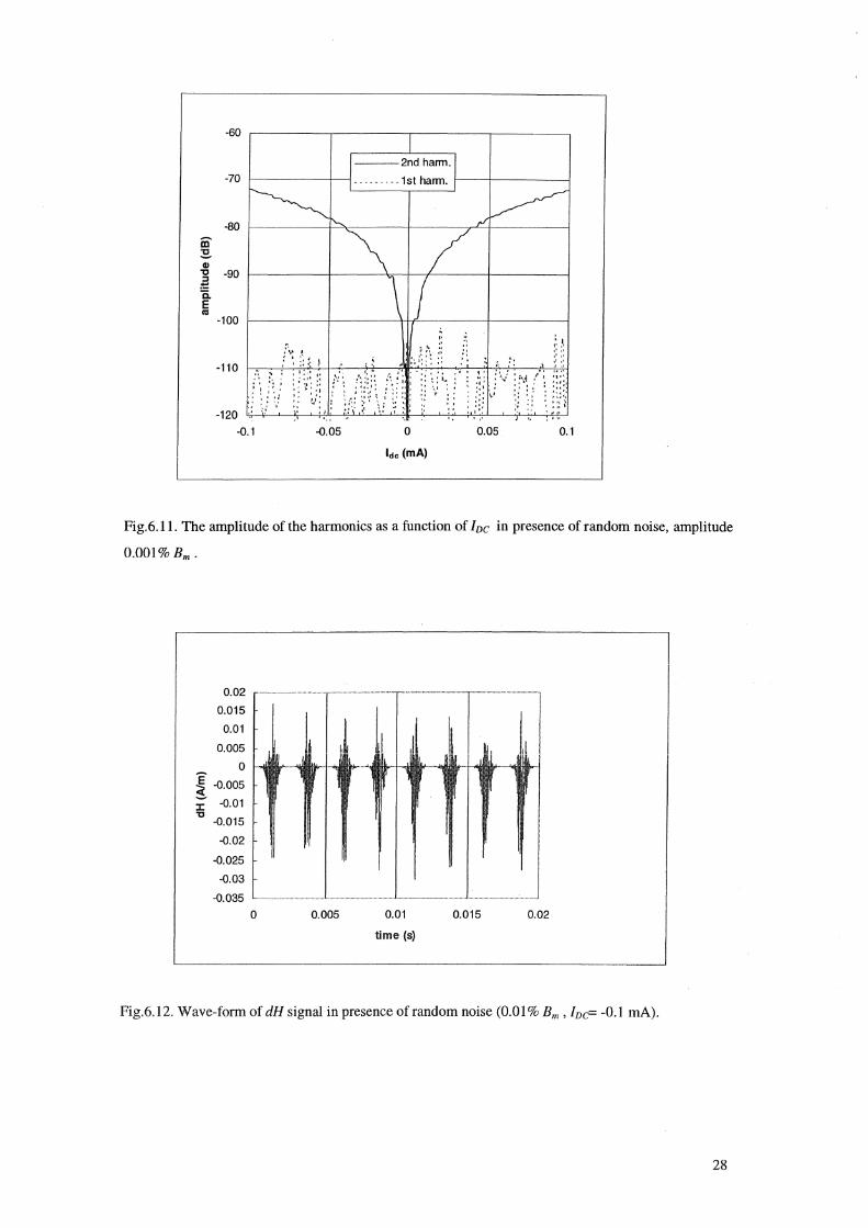
Fig.6.11. The amplitude of the harmonics as a function of Ive in presence of random noise, amplitude

0.001% Bm.

0.02

0.015

0.01

0.005

0 ! -0.005

::c -0.01

"C -0.015

-0.02

-0.025

-0.03

-0.035

!-

0 0.005 0.01

time (s)

0.015 0.02

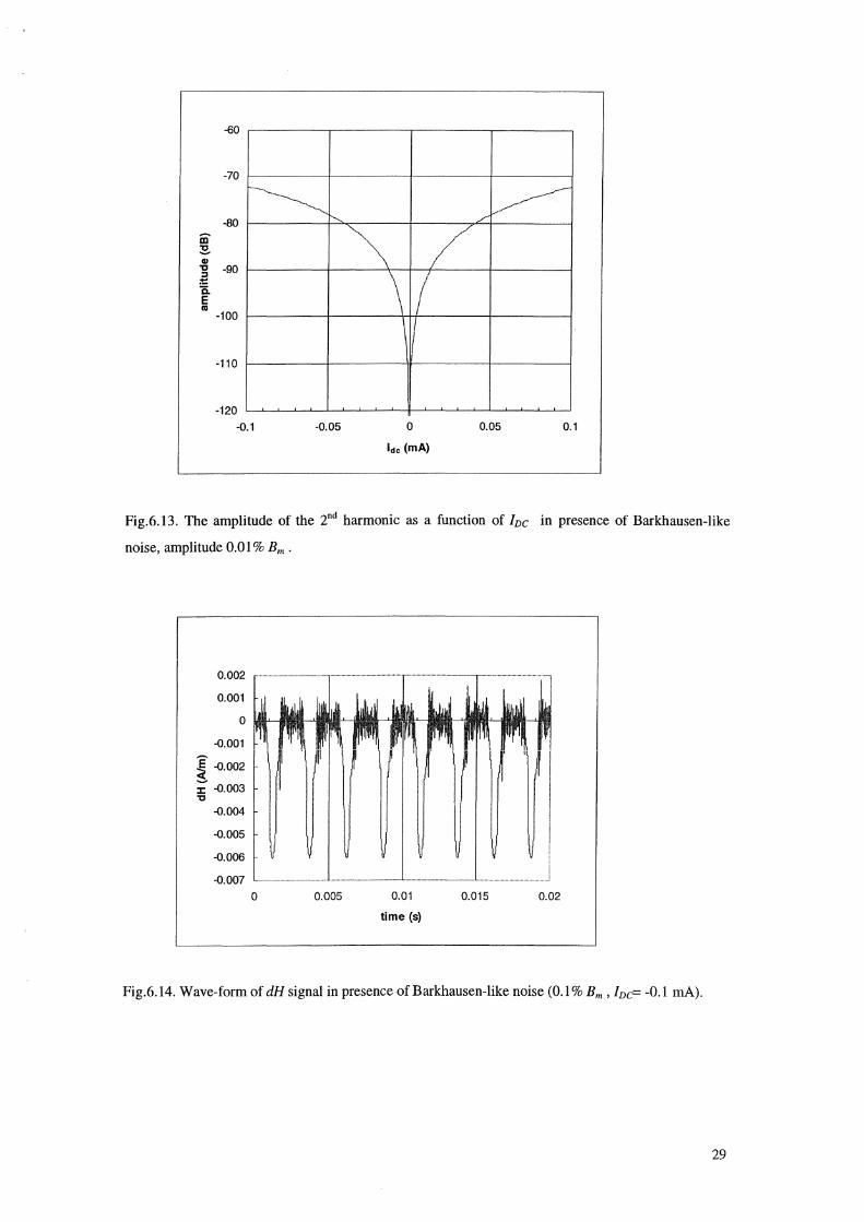
Fig.6.12. Wave-form of dH signal in presence of random noise (0.01 % Bm, /De= -0.1 mA).

28

-60

-70

-80

iii ~ QI ,, -90 j

:!:: "ii. E ca

-100

r~ ~ '- /

~ / \ /

I

-110

-120 -0.1 -0.05 0 0.05 0.1

Ide (mA)

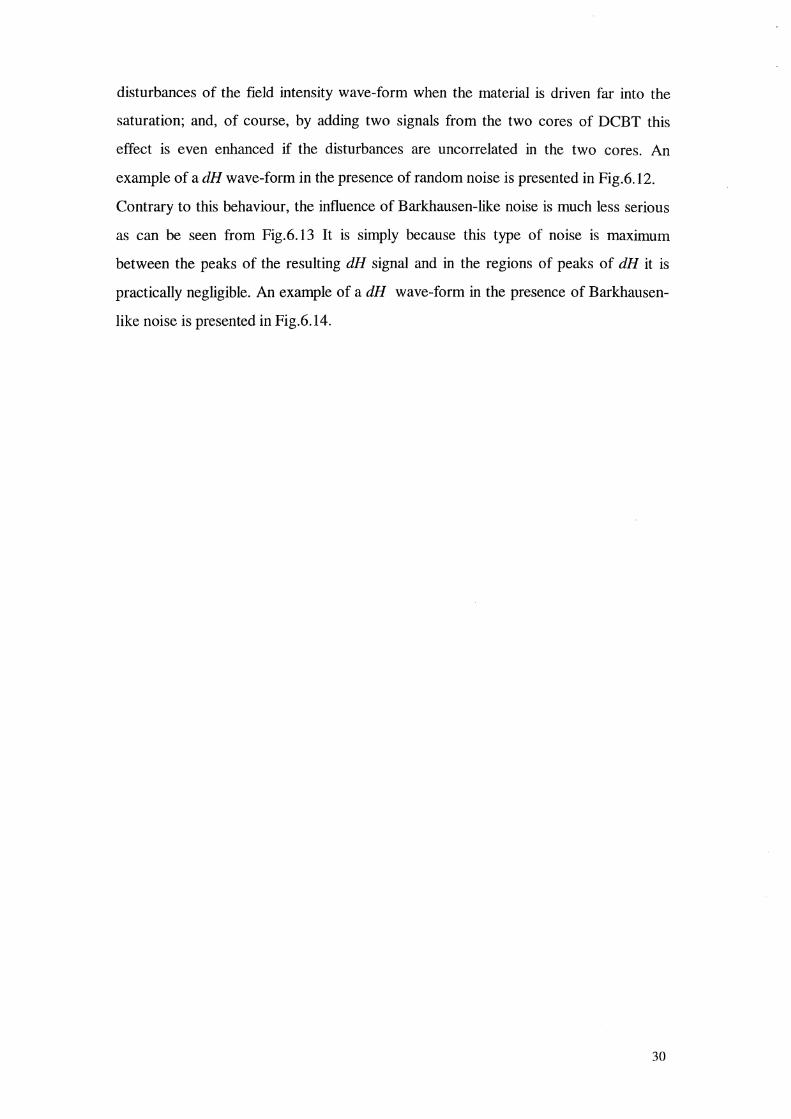
Fig.6.13. The amplitude of the 2"d harmonic as a function of Ive in presence of Barkhausen-like

noise, amplitude 0.01 % Bm .

0.002

0.001

0

-0.001

~ -0.002

;; -0.003 ,, -0.004

-0.005

-0.006

-0.007 ---- -- ------

0 0.005 0.01

time (s)

0.015 0.02

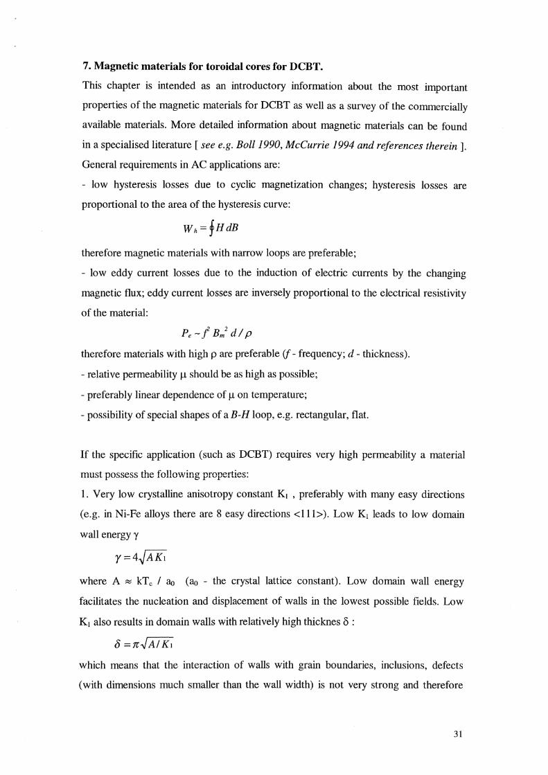
Fig.6.14. Wave-form of dH signal in presence of Barkhausen-like noise (0.1 % Bm, Ive= -0.1 mA).

29

disturbances of the field intensity wave-form when the material is driven far into the

saturation; and, of course, by adding two signals from the two cores of DCBT this

effect is even enhanced if the disturbances are uncorrelated in the two cores. An

example of a dH wave-form in the presence of random noise is presented in Fig.6.12.

Contrary to this behaviour, the influence of Barkhausen-like noise is much less serious

as can be seen from Fig.6.13 It is simply because this type of noise is maximum

between the peaks of the resulting dH signal and in the regions of peaks of dH it is

practically negligible. An example of a dH wave-form in the presence of Barkhausen­

like noise is presented in Fig.6.14.

30

7. Magnetic materials for toroidal cores for DCBT.

This chapter is intended as an introductory information about the most important

properties of the magnetic materials for DCBT as well as a survey of the commercially

available materials. More detailed information about magnetic materials can be found

in a specialised literature [see e.g. Boll 1990, McCurrie 1994 and references therein].

General requirements in AC applications are:

- low hysteresis losses due to cyclic magnetization changes; hysteresis losses are

proportional to the area of the hysteresis curve:

therefore magnetic materials with narrow loops are preferable;

- low eddy current losses due to the induction of electric currents by the changing

magnetic flux; eddy current losses are inversely proportional to the eiectrical resistivity

of the material:

therefore materials with high pare preferable (j - frequency; d - thickness).

- relative permeability µ should be as high as possible;

- preferably linear dependence ofµ on temperature;

- possibility of special shapes of a B-H loop, e.g. rectangular, flat.

If the specific application (such as DCBT) requires very high permeability a material

1. Very low crystalline anisotropy constant K1 , preferably with many easy directions

(e.g. in Ni-Fe alloys there are 8 easy directions <111>). Low K1 leads to low domain

wall energy y

y=4~AK1

where A ~ kTc I ao (ao - the crystal lattice constant). Low domain wall energy

facilitates the nucleation and displacement of walls in the lowest possible fields. Low

K1 also results in domain walls with relatively high thicknes o :

b=n.JAIK1

which means that the interaction of walls with grain boundaries, inclusions, defects

(with dimensions much smaller than the wall width) is not very strong and therefore

31

magnetization changes are not hindered. Low K1 also leads to low coercive field He

and high initial permeability µi because He - Kand µi - 1/K, respectively.

2. High homogeneity: if the magnetic material is single phase material, free from

inclusions, impurities, defects and stresses then in the presence of an applied field the

domains should move easily.

3. Low magnetostriction: the presence of stress produces an effective additional

anisotropy and further impedes the motion of domain walls because of an interaction

between mechanical stress and magnetization (magnetoelastic interaction).

Additional requirements are:

- high Curie temperature

- good temperature stability

- good corrosive resistance

- mechanical strength

- low cost.

High-µ materials can be found in the following groups of materials:

1. Ni-Fe alloys. These materials are well established in all applications requiring

magnetic materials therefore they will be only briefly mentioned here. A range of

compositions over which good magnetic properties can be obtained exists. The highest

µ can be found in 79-80 % Ni materials such as Permalloy (with added Mo),

Supermalloy (79 % Ni, 15 % Fe, 5 % Mo); Mumetal (77 % Ni, 5 % Cu). Various

grades of these alloys are commerciaily avaiiabie from producers such as

Vacuumschmelze GmbH (material with the highestµ - 400 000 - Ultraperm™ 200) or

Imphy S.A. (material with the highestµ - 350 000 - Superrnimphy™ TLS).

2. Amorphous alloys. These materials are usually based on the composition T 80M20

where T is one or more of the transition metals (Fe, Co, Ni, Mo ... ) and M is one or

more of the metalloids or glass forming elements (B, C, Si, P). The alloys are quenched

from the melt which means that there is no regular crystalline structure and

consequently no magnetocrystalline anisotropy energy. Small induced anisotropy can

exist in thin ribbons, but it is very low. As a result y is low and o high which means that

domain walls move easily and very high µ can be achieved. Further increase of µ can

32

be achieved by annealing in order to remove residual stress (via magnetoelasic effects it

impedes domain wall motion). The first commercial alloys were produced by Allied

Signal Corp. - Metglas™, and by Vacuumschmelze GmbH - Vitrovac™. There exist

several groups of these alloys:

1. Fe-based: they have high saturation flux density Bs- 1.4 - 1.8 T;

2. Fe-Ni-based: with Bs- 0.75 - 0.85 T;

3. Co-based: with Bs- 0.4 - 1.2 T, magnetostriction A-1 ~ 0, the highestµ (500 000 for

Vitrovac 6025Z; 1000000 quoted for Metglas 2714A), the lowest losses.

From this it is clear that Bs is very sensitive to the exact composition!

The amorphous alloys are prepared by rapid cooling ( 105 - 106 K/s ) process in which

the melt is injected into (onto) 2 ( 1) cylinders. Due to the nature of this process only

limited thickness (0.02 - 0.05 mm) of the final material (usually in a form of ribbons or

tapes) is available. These materials have very high mechanical hardness (high yielding

point limit) due to the absence of the long range ordering. The mechanical properties

of amorphous magnetic materials allow to use them in the form of flexible foils for the

applications such as magnetic shielding.

3. Nanoncrystalline materials. In composition they resemble the amorphous Fe-based

alloys (roughly T70_80 M30_20 , where T and M are explained above). Their special

properties are set after a crystallization heat treatment. The structure obtained consists

of crystal grains with diameter of cca 10-15 nm surrounded by an amorphous residual

phase. Contrary to amorphous alloys described above the nanocrystalline ribbons are

extremely brittle, therefore only the end product (e.g. a toroidal core) can be heat

treated. Magnetic properties such as permeability, coercivity and core losses are

comparable to amorphous Co-based alloys and thin strip 80%NiFe alloys. As

compared to these materials, nanocrystalline materials have very low magnetostriction,

higher saturation flux density Bs - 1.2 T and better temperature and temporal stability

(especially when compared with amorphous alloys) - the possible permanent

application temperature is up to 150 C. A high value of the Curie temperature tc - 580

C could reduce temperature effects around 20 C and reduce ageing effects. The alloy

contents are also less expensive (compared to Co-based amorphous alloys). A

possibility of very small magnetic domains size (although grain size does not

33

necessarily correlate with the size of domains ) leads to low level of magnetic noise and

good high frequency performance. The present structural phases lead to low or

vanishing saturation magnetostriction which minimises magneto-elastic anisotropy.

Nanocrystalline alloys have relatively high electrical resistivity p - 115 µQcm

(comparable to amorphous alloys) which together with a low ribbon thickness - 20 µm

yields a favourable frequency dependence of µ and low eddy current losses up to 100

kHz (values such as µ1 > 80000 at 1 kHz, µ, > 10000 at 200 kHz can be found in

technical literature).

The main problems of nanocrystalline materials are:

- brittleness as-cast and especially after annealing - it is a consequence of the relatively

low glass-forming ability of the alloy;

- the stress-sensitivity of the magnetic properties which arose from the fact that the

magnetostriction approaches zero only as a result of an internal average (in contrast,

Co-based amorphous alloys are truly non-magnetostrictive almost down to an atomic

scale), as a result nanocrystalline alloys are unsuited to applications such as flexible

shielding.

Commercially available nanocrystalline materials:

• Vitroperm™ - produced by Vaccumschmelze GmbH, products:

- Vitroperm 500F: µ(at H=0.3A/m, 10 kHz)-80 000; Bs-1.2 T, Hc-0.5 Alm, tc -600C,

- Vitroperm 800F: µ(at H=0.3 Alm, 10 kHz) - 100 000

• Finemet™ - produced by Hitachi Metals, products:

- Finemet FT-1: with balanced magnetic characteristics, Bs - 1.35 T, He - 1.3 Alm,

µ1 (lkHz)=70000

- Finemet FT-2: with high Bs, Bs - 1.45 T, He - 1.8 Alm,µ, (lkHz)=50000

- Finemet FT-3: with zero magnetostriction, Bs-1.23 T, Hc-2.5A/m, µ1(lkHz)=70000

- each available with 3 types of the loop: with a high remanence ratio ( B/Bs ); with a

midrange ratio and low ratio (the above data are for midrange).

4. Ferrites. A general formula for the composition of these materials is MO.Fe20 3

where M is bivalent metal ion (Mn, Fe, Co, Ni, Cu, Zn ... ). Most ferrites are oxide

magnetic materials with mechanical properties similar to insulating ceramics. Maximum

permeability and saturation flux density B,,. are lower as compared to those in the above

34

mentioned materials. The important property of ferrites is very high resistivity which

leads to very low eddy current losses. This property makes these materials especially

suitable for high frequency applications.

5. Powder materials. These materials consist of fine powder (Fe or NiFe) insulated

and bounded by binding material. Such a procedure ensures that eddy currents are

reduced in all 3 dimensions (when compared with sheets and foils). The important

property is high isotropic electrical resistivity - factor 104 - 1010 more than metallic

alloys. Similarly to ferrites, these materials are suitable for high frequency applications,

e.g. for cores and various forms elements for radio & TV as well as for power

electronics. The problem can be a relatively high coercive field He which results in high

hysteresis losses.

Comparison of metals, ferrits and powder materials is given in Fig.7.1. (ls is saturation

magnetization).

J,(T) -j µ.

(<Hn;m)~ 1~' ~ 2.5

2.0j 10' j 10'1 1.5 104 1010

1.0 103 106

0.5 102 102

1

0 10 10-2

metals 0 powders ferrites

Fig.7.1. Magnetic and electrical properties of soft magnetic materials (after Boll 1990).

35

Acknowledgments.

I would like to express my thanks to Mr.Gelato for his help in introducing me to the

problems of beam transformers as well as for fruitful discussions and motivating

suggestions during all the work on this project. The help of Patrick Odier in all

practical aspects of the project is also greatly appreciated. Paolo Maccarini was

very helpful at the beginning of experiments with AC+DC field superposition. I am

very grateful also to Jacques Longo for his friendly collaboration.

References:

[ Andersson 1994 ] Y.Andersson: Preliminary Study of the Beam Transformer

Prototype for the LHC at CERN ... December 1994 (not published).

[Boll 1990] - R.Boll: Weichmagnetische Werkstoffe, Vacuumschnelze GmbH Hanau

1990.

[Borer & Jung 1984] - I.Borer & R.Iung: Diagnostics, CAS CERN 84-15, 1984.

[ Cortial 1997] - F.Cortial et al., IEEE Trans. Magn. MAG-33 (1997) 1592.

[ Gelato 1992 ] - G.Gelato: Beam Transformers, in Beam Instrumentation, ed.

I.Bosser, CERN 92-00 ED, 1992.

[Koziol 1989] - H.Koziol: Beam Diagnostics, CERN/PS 89-09 (AR), 1989.

[Koziol 1995] - H.Koziol: Diagnostics for Low Intensity Beams, CERN/PS 95-23

[ McCurrie 1994 ] - R.A.McCurrie: Ferromagnetic Materials: Structure and

Properties, Academic Press London 1994.

[ Odier & Maccarini 1997] - P.Odier & P.Maccarini: CERN PS/BD/Note 96-09

[Philips 1994] - D.A.Philips et al., IEEE Trans. Magn. MAG-30 (1994) 4377.

[Rivas 1981] - I Rivas et al., IEEE Trans. Magn. MAG-17 (1981) 1498.

[ Say 1954 ] - M.G.Say (ed): Magnetic Amplifiers and Saturable Reactors, George

Newness Ltd., London 1954.

[Scouten 1972] - D.C.Scouten, IEEE Trans. Magn. MAG-8 (1972) 223.

[Swartzendruber 1990] - L.J.Swartzendruber et al., I.Appl.Phys. 67 (1990) 5469.

[Unser 1969] - K.Unser: IEEE Trans.Nucl.Sci. NS-16 (1969) 934.

[Unser 1981] - K.Unser: IEEE Trans.Nucl.Sci. NS-28 (1981) 2344.

[ Unser 1989 ] - K.Unser: in Proc. IEEE Particle Accelerator Conference, Chicago

1989

[Unser 1991] - K.Unser: CERN SL/91-42 (BI).

[ Unser 1993] - K.Unser: CERN PS/93-35 (BD).

[Scouten 1970] - D.C.Scouten, IEEE Trans. Magn. MAG-6 (1970) 383.

[Vos 1994] - L.Vos: CERN SL/94-74 (BI).