Then Versus Now: A Comparison of Total Scheme Complexity

Bob Morris, Roy Moxley, and Christina Kusch Schweitzer Engineering Laboratories, Inc.

Presented at the 1st Annual Protection, Automation and Control World Conference

Dublin, Ireland June 21–24, 2010

Previously presented at the 9th Annual Clemson University Power Systems Conference, March 2010,

45th Annual Minnesota Power Systems Conference, November 2009, and 36th Annual Western Protective Relay Conference, October 2009

Originally presented at the 62nd Annual Conference for Protective Relay Engineers, March 2009

1

Then Versus Now: A Comparison of Total Scheme Complexity

Bob Morris, Roy Moxley, and Christina Kusch, Schweitzer Engineering Laboratories, Inc.

Abstract—Today’s protection engineer is not at a loss for things to do. New and retrofit projects along with added system requirements have increased the workload for designing, setting, installing, and maintaining protection systems. It is not uncom-mon for engineers to look back at the “good old days” with nostalgia.

This paper performs a component-by-component and line-by-line comparison of protection schemes from the electromechani-cal, microprocessor, and distributed microprocessor architec-tures. For a complete line protection system, the comparison includes the protective relays, auxiliary logic, settings, firmware reliability, wiring, and testing (both periodic and scheme).

Recognizing that engineers want only the best, yet practically attainable protection system, this paper includes measurements and calculations of reliability to bring a scheme online. Fault tree analysis techniques are used to bring numerical values to scheme comparisons.

Finally, observations regarding functional requirements of old and modern systems allow engineers and management to eva-luate the technological effectiveness of overall control systems.

I. INTRODUCTION Baseball great Yogi Berra is quoted as saying, “If you

don’t know where you are going, you will wind up somewhere else.” This is certainly applicable in the world of protective relays. In the past 25 years, we have gone from collections of black boxes filled with magnets and springs to microprocessor-based schemes, combining the functions of dozens of relays into one package. As an industry, we are looking at further consolidation of devices and added options in configuration. The question that we need to address is: Are we making progress?

Rather than a vague, subjective measurement of progress, we can use mathematical tools to examine the probability of favorable or unfavorable results. In this way, we can plan and take design actions to improve the probability of desired outcomes.

II. FAULT TREE ANALYSIS A useful way to measure probability is through fault tree

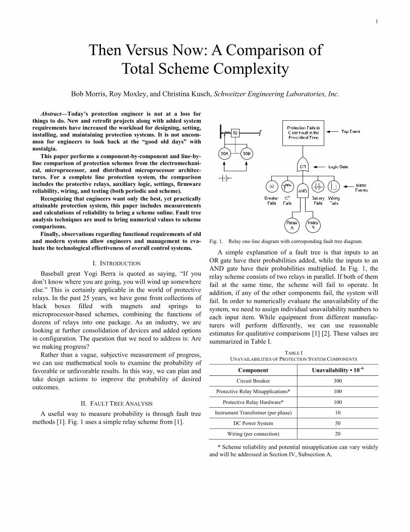
methods [1]. Fig. 1 uses a simple relay scheme from [1].

Fig. 1. Relay one-line diagram with corresponding fault tree diagram.

A simple explanation of a fault tree is that inputs to an OR gate have their probabilities added, while the inputs to an AND gate have their probabilities multiplied. In Fig. 1, the relay scheme consists of two relays in parallel. If both of them fail at the same time, the scheme will fail to operate. In addition, if any of the other components fail, the system will fail. In order to numerically evaluate the unavailability of the system, we need to assign individual unavailability numbers to each input item. While equipment from different manufac-turers will perform differently, we can use reasonable estimates for qualitative comparisons [1] [2]. These values are summarized in Table I.

TABLE I UNAVAILABILITIES OF PROTECTION SYSTEM COMPONENTS

Component Unavailability • 10–6

Circuit Breaker 300

Protective Relay Misapplications* 100

Protective Relay Hardware* 100

Instrument Transformer (per phase) 10

DC Power System 50

Wiring (per connection) 20

* Scheme reliability and potential misapplication can vary widely and will be addressed in Section IV, Subsection A.

2

Note that the unavailability numbers in Table I are only estimates and can vary depending on operating and testing practices. The wiring unavailability in particular assumes correction of errors detected by wiring checks, but this could be improved by practices, such as trip circuit monitoring [2]. In the final scheme evaluation, shown later in Table V, we will give a range from 2 to 20 • 10–6 to show the impact on scheme unavailability. In Fig. 1, we show relay failure as a single probability, but it is actually the sum of hardware, misapplication, and firmware unavailability. The Fig. 1 diagram is different than the diagram that would be used for a false trip as the top event. In the analysis of this paper, we are using a failure to trip for consistency reasons. The same analysis techniques could be used to evaluate the probability of false trips.

Relay engineers upgrade firmware on protective relays to enhance features and correct defects. One relay manufacturer tracks a relay maintenance indicator that is a measure of the rate at which a protection engineer upgrades device firmware to correct a defect. Based on this manufacturer’s field experience, a firmware reliability measure of 30 years mean time to firmware defect upgrade is conservative. Field experience also suggests a one day mean time to repair (MTTR) per relay firmware upgrade. These data give microprocessor-based device firmware an unavailability of 90 • 10–6.

In our calculations, we add each item separately. Assuming a simple protection scheme, we have 32 wiring connections (three CTs [current transformers], one dc/trip • four wire segments each, including test block and terminal block), which leads to the following scheme failure calculation:

(Breaker Failure) + (CT Failure) + [(Relay A Failure + Relay A Misapplication + Relay A Firmware Upgrade) • (Relay B Failure + Relay B Misapplication + Relay B Firmware Upgrade)] + (DC Failure) + (32 • Wire Failure) = Scheme Failure

Combining and evaluating terms can give us Table II, an application-specific version of Table I.

TABLE II UNAVAILABILITY OF PROTECTION COMPONENTS FOR FIG. 1 SCHEME

Component Unavailability

Circuit Breaker, Instrument Transformers, DC Connection

(300 • 10–6) + (3 • 10 • 10–6) + (50 • 10–6) 0.00038

Relay Scheme (100 • 10–6 + 100 • 10–6 + 91 • 10–6) • (100 • 10–6 + 100 • 10–6 + 90 • 10–6) 0.00000008

Wiring System 32 • 20 • 10–6 0.00064

Total 0.00038 + 0.0000008 + 0.00064 0.0010208

With this component grouping, we see that even with a minimal, 32-wire connecting system, the wiring becomes the limiting factor in improving the availability.

III. SCHEME COMPARISON Evaluating a more complex scheme is possible using the

same techniques with consideration for the different types of relays involved. In this case, we compare an electromechani-cal distance scheme, including reclosing and synchronism check, with a modern microprocessor relay [3].

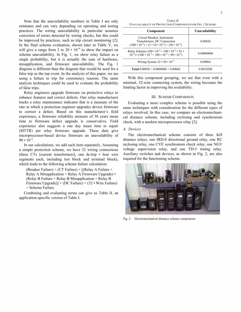
A. Devices The electromechanical scheme consists of three KD

distance relays, one IRD-8 directional ground relay, one RC reclosing relay, one CVE synchronism check relay, one NGV voltage supervision relay, and one TD-5 timing relay. Auxiliary switches and devices, as shown in Fig. 2, are also required for the functioning scheme.

Fig. 2. Electromechanical distance scheme components.

3

The microprocessor relay is a single relay with multiple I/O included, as well as additional functions.

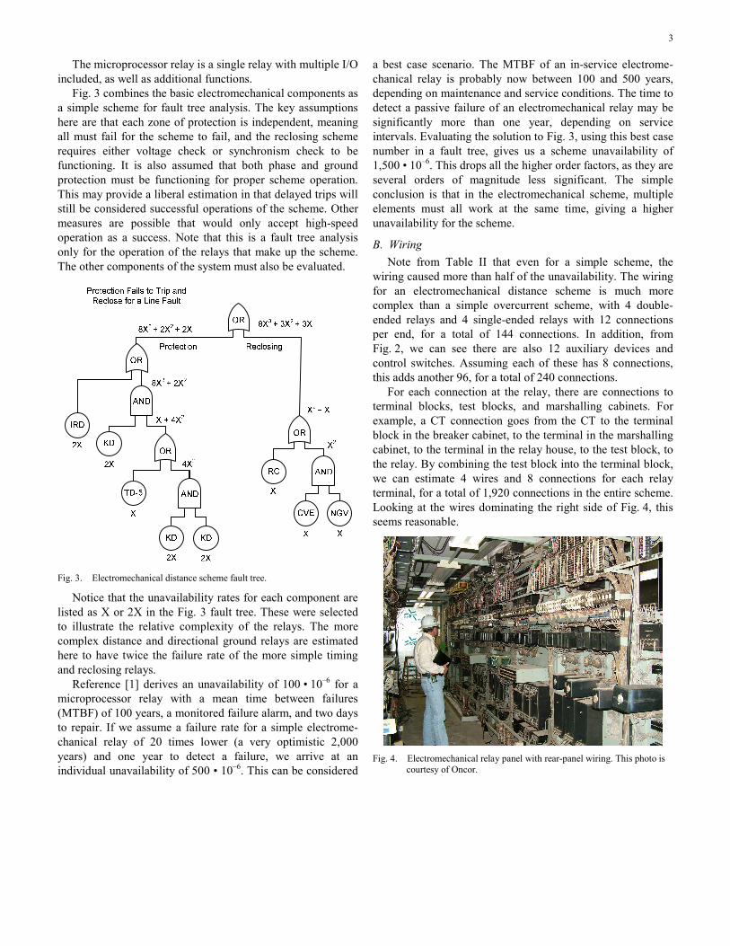
Fig. 3 combines the basic electromechanical components as a simple scheme for fault tree analysis. The key assumptions here are that each zone of protection is independent, meaning all must fail for the scheme to fail, and the reclosing scheme requires either voltage check or synchronism check to be functioning. It is also assumed that both phase and ground protection must be functioning for proper scheme operation. This may provide a liberal estimation in that delayed trips will still be considered successful operations of the scheme. Other measures are possible that would only accept high-speed operation as a success. Note that this is a fault tree analysis only for the operation of the relays that make up the scheme. The other components of the system must also be evaluated.

Fig. 3. Electromechanical distance scheme fault tree.

Notice that the unavailability rates for each component are listed as X or 2X in the Fig. 3 fault tree. These were selected to illustrate the relative complexity of the relays. The more complex distance and directional ground relays are estimated here to have twice the failure rate of the more simple timing and reclosing relays.

Reference [1] derives an unavailability of 100 • 10–6 for a microprocessor relay with a mean time between failures (MTBF) of 100 years, a monitored failure alarm, and two days to repair. If we assume a failure rate for a simple electrome-chanical relay of 20 times lower (a very optimistic 2,000 years) and one year to detect a failure, we arrive at an individual unavailability of 500 • 10–6. This can be considered

a best case scenario. The MTBF of an in-service electrome-chanical relay is probably now between 100 and 500 years, depending on maintenance and service conditions. The time to detect a passive failure of an electromechanical relay may be significantly more than one year, depending on service intervals. Evaluating the solution to Fig. 3, using this best case number in a fault tree, gives us a scheme unavailability of 1,500 • 10–6. This drops all the higher order factors, as they are several orders of magnitude less significant. The simple conclusion is that in the electromechanical scheme, multiple elements must all work at the same time, giving a higher unavailability for the scheme.

B. Wiring Note from Table II that even for a simple scheme, the

wiring caused more than half of the unavailability. The wiring for an electromechanical distance scheme is much more complex than a simple overcurrent scheme, with 4 double-ended relays and 4 single-ended relays with 12 connections per end, for a total of 144 connections. In addition, from Fig. 2, we can see there are also 12 auxiliary devices and control switches. Assuming each of these has 8 connections, this adds another 96, for a total of 240 connections.

For each connection at the relay, there are connections to terminal blocks, test blocks, and marshalling cabinets. For example, a CT connection goes from the CT to the terminal block in the breaker cabinet, to the terminal in the marshalling cabinet, to the terminal in the relay house, to the test block, to the relay. By combining the test block into the terminal block, we can estimate 4 wires and 8 connections for each relay terminal, for a total of 1,920 connections in the entire scheme. Looking at the wires dominating the right side of Fig. 4, this seems reasonable.

Fig. 4. Electromechanical relay panel with rear-panel wiring. This photo is courtesy of Oncor.

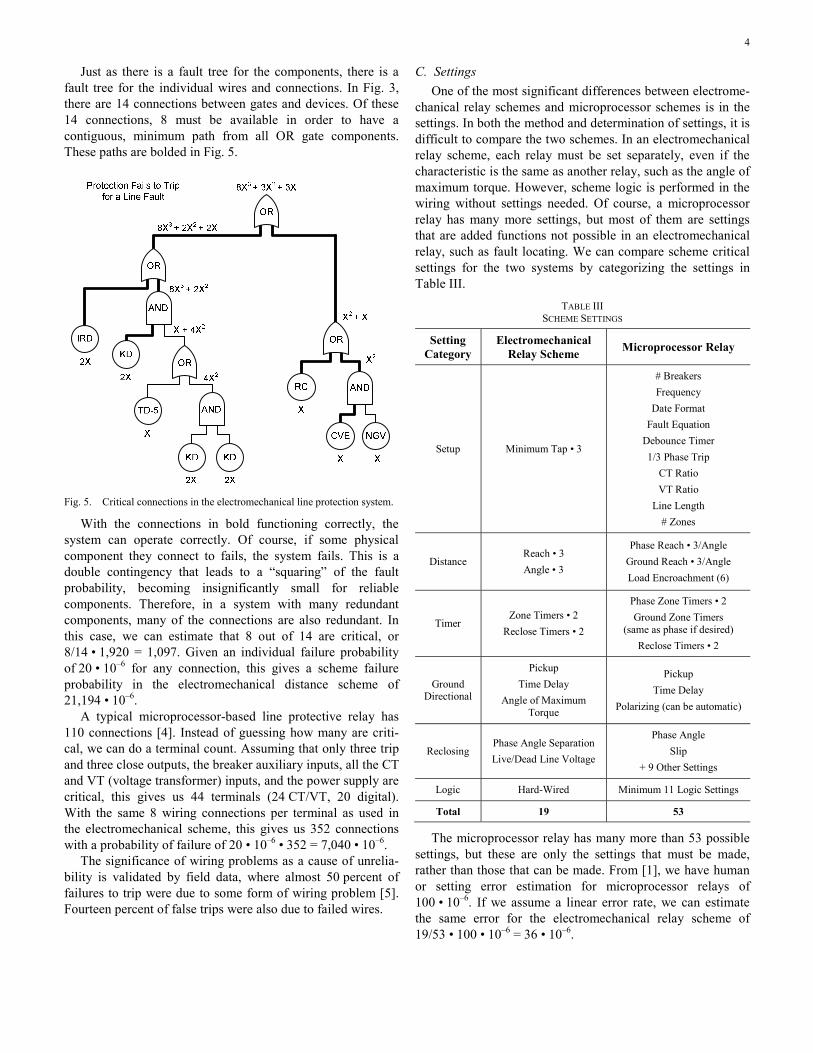
4

Just as there is a fault tree for the components, there is a fault tree for the individual wires and connections. In Fig. 3, there are 14 connections between gates and devices. Of these 14 connections, 8 must be available in order to have a contiguous, minimum path from all OR gate components. These paths are bolded in Fig. 5.

Fig. 5. Critical connections in the electromechanical line protection system.

With the connections in bold functioning correctly, the system can operate correctly. Of course, if some physical component they connect to fails, the system fails. This is a double contingency that leads to a “squaring” of the fault probability, becoming insignificantly small for reliable components. Therefore, in a system with many redundant components, many of the connections are also redundant. In this case, we can estimate that 8 out of 14 are critical, or 8/14 • 1,920 = 1,097. Given an individual failure probability of 20 • 10–6 for any connection, this gives a scheme failure probability in the electromechanical distance scheme of 21,194 • 10–6.

A typical microprocessor-based line protective relay has 110 connections [4]. Instead of guessing how many are criti-cal, we can do a terminal count. Assuming that only three trip and three close outputs, the breaker auxiliary inputs, all the CT and VT (voltage transformer) inputs, and the power supply are critical, this gives us 44 terminals (24 CT/VT, 20 digital). With the same 8 wiring connections per terminal as used in the electromechanical scheme, this gives us 352 connections with a probability of failure of 20 • 10–6 • 352 = 7,040 • 10–6.

The significance of wiring problems as a cause of unrelia-bility is validated by field data, where almost 50 percent of failures to trip were due to some form of wiring problem [5]. Fourteen percent of false trips were also due to failed wires.

C. Settings One of the most significant differences between electrome-

chanical relay schemes and microprocessor schemes is in the settings. In both the method and determination of settings, it is difficult to compare the two schemes. In an electromechanical relay scheme, each relay must be set separately, even if the characteristic is the same as another relay, such as the angle of maximum torque. However, scheme logic is performed in the wiring without settings needed. Of course, a microprocessor relay has many more settings, but most of them are settings that are added functions not possible in an electromechanical relay, such as fault locating. We can compare scheme critical settings for the two systems by categorizing the settings in Table III.

TABLE III SCHEME SETTINGS

Setting Category

Electromechanical Relay Scheme Microprocessor Relay

Setup Minimum Tap • 3

# Breakers Frequency

Date Format Fault Equation

Debounce Timer 1/3 Phase Trip

CT Ratio VT Ratio

Line Length # Zones

Distance Reach • 3 Angle • 3

Phase Reach • 3/Angle Ground Reach • 3/Angle Load Encroachment (6)

Timer Zone Timers • 2

Reclose Timers • 2

Phase Zone Timers • 2 Ground Zone Timers

(same as phase if desired) Reclose Timers • 2

Ground Directional

Pickup Time Delay

Angle of Maximum Torque

Pickup Time Delay

Polarizing (can be automatic)

Reclosing Phase Angle Separation Live/Dead Line Voltage

Phase Angle Slip

+ 9 Other Settings

Logic Hard-Wired Minimum 11 Logic Settings

Total 19 53

The microprocessor relay has many more than 53 possible settings, but these are only the settings that must be made, rather than those that can be made. From [1], we have human or setting error estimation for microprocessor relays of 100 • 10–6. If we assume a linear error rate, we can estimate the same error for the electromechanical relay scheme of 19/53 • 100 • 10–6 = 36 • 10–6.

5

There is still the question of how we account for the complexity of approximately 10,000 additional settings that may be possible to make in a microprocessor relay. A close look at these settings makes them far less intimidating, since hundreds of the settings are identifications that are convenient but not essential. Additional hundreds of settings involve communications that will be immediately detected as nonfunctioning if they are incorrect. Perhaps the largest category of additional settings is the extra settings groups available in microprocessor relays. Typical relays include six groups, five more than an electromechanical scheme. These are typically used for special or alternate circumstances that involve the change of only a few settings from Group 1. Even though each group has hundreds of settings, because most of them are copied, only a few introduce the possibility of errors.

The last factors that reduce the possibility of errors in settings are the checks involved in performing those settings. While there is no self-test in an electromechanical relay to determine that the current required to enter the reach setting is not in conflict with another supervising overcurrent element, setting conflicts are detected in microprocessor relays. Reference [2] points out that wiring errors are reduced from 1/500 to 1/50,000 by installation testing. Likewise, consistency checks in setting software can reduce errors by orders of magnitude.

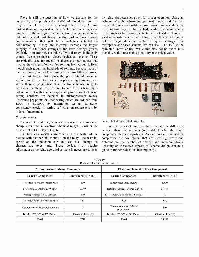
D. Adjustments The need to make adjustments is a result of component

change over time in electromechanical relays. Consider the disassembled KD relay in Fig. 6.

Six slide wire resisters are visible in the center of the picture with another still mounted on the relay. The restraint spring on the induction cup unit can also change its characteristic over time. These devices may require adjustment as the relay ages. Adjustment is necessary to keep

the relay characteristics as set for proper operation. Using an estimate of eight adjustments per major relay and four per minor relay is a reasonable approximation. Some slide wires may not ever need to be touched, while other maintenance items, such as burnishing contacts, are not added. This will yield 48 adjustments for the scheme. Since this is on the same order of magnitude as the number of required settings in the microprocessor-based scheme, we can use 100 • 10–6 as the estimated unavailability. While this may not be exact, it is probably within reasonable proximity of the right value.

Fig. 6. KD relay partially disassembled.

It is not the exact numbers that illustrate the difference between these two schemes (see Table IV) but the major components that are significant. As measures of total scheme complexity, the two factors that are most significant and different are the number of devices and interconnections. Focusing on these two aspects of scheme design can be a guide to further reductions in complexity.

TABLE IV DISTANCE SCHEME UNAVAILABILITY

Microprocessor Scheme Component Electromechanical Scheme Component

Scheme Component Unavailability (• 10–6) Scheme Component Unavailability (• 10–6)

Microprocessor Device Hardware 100 Electromechanical Relays 1,500

Microprocessor Scheme Wiring 7,040 Electromechanical Scheme Wiring 21,194

Microprocessor Relay Settings 100 Electromechanical Scheme Settings 36

Microprocessor Device Firmware 90 N/A N/A

Microprocessor Relay Adjustments 0 Electromechanical Scheme Adjustments 100

Breaker, CT, VT, or DC Failure 380 (from Table II) Breaker, CT, VT, or DC Failure 380 (from Table II)

Total 7710 Total 23,210

6

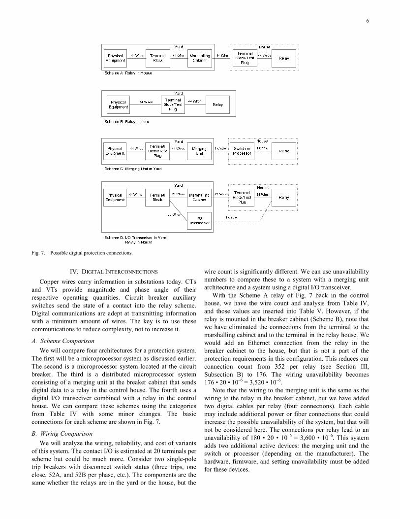
Fig. 7. Possible digital protection connections.

IV. DIGITAL INTERCONNECTIONS Copper wires carry information in substations today. CTs

and VTs provide magnitude and phase angle of their respective operating quantities. Circuit breaker auxiliary switches send the state of a contact into the relay scheme. Digital communications are adept at transmitting information with a minimum amount of wires. The key is to use these communications to reduce complexity, not to increase it.

A. Scheme Comparison We will compare four architectures for a protection system.

The first will be a microprocessor system as discussed earlier. The second is a microprocessor system located at the circuit breaker. The third is a distributed microprocessor system consisting of a merging unit at the breaker cabinet that sends digital data to a relay in the control house. The fourth uses a digital I/O transceiver combined with a relay in the control house. We can compare these schemes using the categories from Table IV with some minor changes. The basic connections for each scheme are shown in Fig. 7.

B. Wiring Comparison We will analyze the wiring, reliability, and cost of variants

of this system. The contact I/O is estimated at 20 terminals per scheme but could be much more. Consider two single-pole trip breakers with disconnect switch status (three trips, one close, 52A, and 52B per phase, etc.). The components are the same whether the relays are in the yard or the house, but the

wire count is significantly different. We can use unavailability numbers to compare these to a system with a merging unit architecture and a system using a digital I/O transceiver.

With the Scheme A relay of Fig. 7 back in the control house, we have the wire count and analysis from Table IV, and those values are inserted into Table V. However, if the relay is mounted in the breaker cabinet (Scheme B), note that we have eliminated the connections from the terminal to the marshalling cabinet and to the terminal in the relay house. We would add an Ethernet connection from the relay in the breaker cabinet to the house, but that is not a part of the protection requirements in this configuration. This reduces our connection count from 352 per relay (see Section III, Subsection B) to 176. The wiring unavailability becomes 176 • 20 • 10–6 = 3,520 • 10–6.

Note that the wiring to the merging unit is the same as the wiring to the relay in the breaker cabinet, but we have added two digital cables per relay (four connections). Each cable may include additional power or fiber connections that could increase the possible unavailability of the system, but that will not be considered here. The connections per relay lead to an unavailability of 180 • 20 • 10–6 = 3,600 • 10–6. This system adds two additional active devices: the merging unit and the switch or processor (depending on the manufacturer). The hardware, firmware, and setting unavailability must be added for these devices.

7

The digital I/O transceiver eliminates the digital wires at the cost of an additional device.

The tabulated unavailability of each scheme is shown in Table V.

Some manufacturers list an MTBF of as low as 30 years, which increases the unavailability of a scheme involving those components. This increased unavailability is shown in the second set of numbers in the Separate Merging Unit column of Table V. Note that this higher unavailability brings the scheme unavailability of the Separate Merging Unit system closer to that of the scheme using I/O transceivers.

The third set of numbers reduces the wiring error rate from 20 per million to 2 per million. This could reflect the use of very careful wiring checks and a trip circuit monitoring scheme. Note that this makes the active device component much more significant in the comparison.

This analysis does not include the inconvenience of the test plugs being in the yard for Schemes B and C. Additionally, the test set for Scheme C (merging unit in yard) is in a different location than the relay. Costs of the schemes must also be considered. Because wire and devices add cost and increase unavailability, the relative “scores” of Table V can also be considered proportional to total installed system cost.

TABLE V DIGITAL SCHEME UNAVAILABILITY

Relay in House Relay in Yard Separate Merging Unit I/O Transceiver

Scheme Component

Unavailability (• 10–6)

Scheme Component

Unavailability(• 10–6)

Scheme Component

Unavailability(• 10–6)

Scheme Component

Unavailability(• 10–6)

Relay Hardware 100/333 Relay

Hardware 100/333 Merging Unit Hardware 100/333 Relay

Hardware 100/333

Relay Firmware 90 Relay

Firmware 90 Merging Unit Firmware 90 Relay

Firmware 90

Switch Hardware 100/333 Digital I/O

Hardware 100

Switch/

Processor Settings

90

Switch/

Processor Firmware

90

Relay Hardware 100/333

Relay Firmware 90

House Relay Wiring

(176 wires) *second

number uses 2 • 10–6

per connection

7,040/704 Breaker Relay

Wiring (88 wires)

3,520/352

Breaker to Merging Unit

to Relay Wiring

(88 wires, 2 cables)

3,600/360

Breaker to I/O to House Wiring

(136 wires, 1 cable)

5,480/548

Relay Settings 100 Relay Settings 100 Relay Settings 100 Relay Settings 100

Breaker, CT, VT, or DC

Failure

380 (from Table II)

Breaker, CT, VT, or DC

Failure

380 (from Table II)

Breaker, CT, VT, or DC

Failure

380 (from Table II)

Breaker, CT, VT, or DC

Failure

380 (from Table II)

Total 7,710/7,943/1607 4,190/4,423/1,255 4,740/5,439/2,199 6,250/6,483/1,551

8

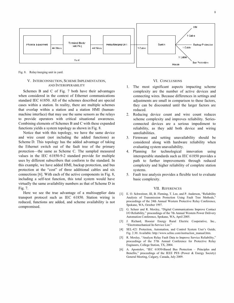
Fig. 8. Relay/merging unit in yard.

V. INTERCONNECTION, SCHEME IMPLEMENTATION, AND INTEROPERABILITY

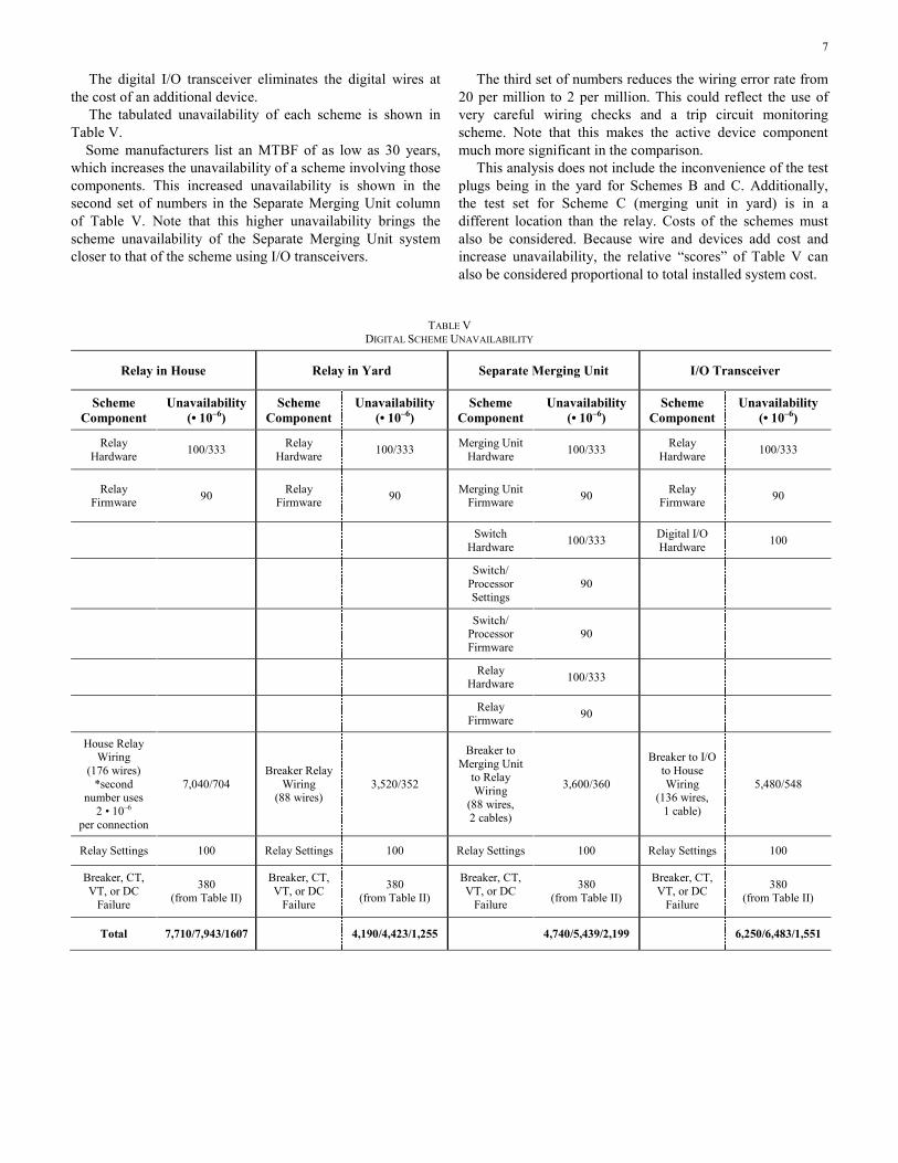
Schemes B and C of Fig. 7 both have their advantages when considered in the context of Ethernet communications standard IEC 61850. All of the schemes described are special cases within a station. In reality, there are multiple schemes that overlap within a station and a station HMI (human-machine interface) that may use the same sensors as the relays to provide operators with critical situational awareness. Combining elements of Schemes B and C with these expanded functions yields a system topology as shown in Fig. 8.

Notice that with this topology, we have the same device and wire count (not including the added functions) as Scheme D. This topology has the added advantage of taking the Ethernet switch out of the fault tree of the primary protection—the same as Scheme C. The sampled measured values in the IEC 61850-9-2 standard provide for multiple uses by different subscribers that conform to the standard. In this example, we have added HMI, backup protection, and bus protection at the “cost” of three additional cables and six connections [6]. With each of the active components in Fig. 8, including a self-test function, this total system would have virtually the same availability numbers as that of Scheme D in Fig. 7.

Here we see the true advantage of a multisupplier data transport protocol such as IEC 61850. Station wiring is reduced, functions are added, and scheme availability is not compromised.

VI. CONCLUSIONS 1. The most significant aspects impacting scheme

complexity are the number of active devices and connecting wires. Because differences in settings and adjustments are small in comparison to these factors, they can be discounted until the larger factors are reduced.

2. Reducing device count and wire count reduces scheme complexity and improves reliability. Series-connected devices are a serious impediment to reliability, as they add both device and wiring unreliabilities.

3. Firmware and setting unavailability should be considered along with hardware reliability when evaluating system unavailability.

4. Planning for technological innovation using interoperable standards such as IEC 61850 provides a path to further improvements through reduced complexity and higher reliability of complete station systems.

5. Fault tree analysis provides a flexible tool to evaluate basic complexity.

VII. REFERENCES [1] E. O. Schweitzer, III, B. Fleming, T. Lee, and P. Anderson, “Reliability

Analysis of Transmission Protection Using Fault Tree Methods,” proceedings of the 24th Annual Western Protective Relay Conference, Spokane, WA, October 1997.

[2] G. Scheer and R. Moxley, “Digital Communications Improve Contact I/O Reliability,” proceedings of the 7th Annual Western Power Delivery Automation Conference, Spokane, WA, April 2005.

[3] J. Richard, Hoosier Energy Rural Electric Cooperative, Inc., “Electromechanical In-Service List.”

[4] SEL-421 Protection, Automation, and Control System User’s Guide, Fig. 2.30. Available: http://www.selinc.com/instruction_manual.htm.

[5] R. Moxley, “Analyze Relay Fault Data to Improve Service Reliability,” proceedings of the 57th Annual Conference for Protective Relay Engineers, College Station, TX, 2004.

[6] A. Apostolov, “IEC 61850-Based Bus Protection – Principles and Benefits,” proceedings of the IEEE PES (Power & Energy Society) General Meeting, Calgary, Canada, July 2009.

9

VIII. BIOGRAPHIES

Bob Morris received his B.S. in Geophysical Engineering from Montana Tech in 1984 and an M.S. in Engineering Science from Montana Tech in 1991. He worked for Montana Power Company in substation and generation plant automation from 1987 to 1991. In 1991, he joined Schweitzer Engineering Laboratories, Inc. (SEL) as a firmware design engineer. He has designed and led the development of several protective relay platforms. His interests are protective relay design, product quality and reliability, and engineering development process improvement. He is presently research and development director at SEL.

Roy Moxley has a B.S. in Electrical Engineering from the University of Colorado. He joined Schweitzer Engineering Laboratories, Inc. (SEL) in 2000 and serves as marketing manager for protection products. Prior to joining SEL, he was with General Electric Company as a relay application engineer, transmission and distribution (T&D) field application engineer, and T&D account manager. He is a registered professional engineer in the State of Pennsylvania and has authored numerous technical papers presented at U.S. and international relay and automation conferences.

Christina Kusch has a B.S. in Electrical Engineering from the University of California, Los Angeles. She joined Schweitzer Engineering Laboratories, Inc. in 2007 and serves as an associate product manager for substation protection products. She is a member of IEEE and the IEEE Power & Energy Society.

Previously presented at the 2009 Texas A&M Conference for Protective Relay Engineers.

© 2009 IEEE – All rights reserved.20090911 • TP6356-01