the$memory$hierarchy$ - hacettepe · 1 the$memory$hierarchy$ $ fall$2012$ instructors:$$...

1

The Memory Hierarchy Fall 2012

Instructors: Aykut & Erkut Erdem

Acknowledgement: The course slides are adapted from the slides prepared by R.E. Bryant, D.R. O’Hallaron, G. Kesden and Markus Püschel of Carnegie-‐Mellon Univ.

3

Today ¢  Storage technologies and trends ¢  Locality of reference ¢  Caching in the memory hierarchy ¢  Cache memory organiza?on and opera?on ¢  Performance impact of caches

§  The memory mountain §  Rearranging loops to improve spaOal locality §  Using blocking to improve temporal locality

4

Random-‐Access Memory (RAM) ¢  Key features

§  RAM is tradiOonally packaged as a chip. §  Basic storage unit is normally a cell (one bit per cell). §  MulOple RAM chips form a memory.

¢  Sta?c RAM (SRAM) §  Each cell stores a bit with a four or six-‐transistor circuit. §  Retains value indefinitely, as long as it is kept powered. §  RelaOvely insensiOve to electrical noise (EMI), radiaOon, etc. §  Faster and more expensive than DRAM.

¢  Dynamic RAM (DRAM) §  Each cell stores bit with a capacitor. One transistor is used for access §  Value must be refreshed every 10-‐100 ms. §  More sensiOve to disturbances (EMI, radiaOon,…) than SRAM. §  Slower and cheaper than SRAM.

5

SRAM vs DRAM Summary

Trans. Access Needs Needs per bit time refresh? EDC? Cost Applications

SRAM 4 or 6 1X No Maybe 100x Cache memories DRAM 1 10X Yes Yes 1X Main memories,

frame buffers

6

Conven?onal DRAM Organiza?on ¢  d x w DRAM:

§  dw total bits organized as d supercells of size w bits

cols

rows

0 1 2 3

0

1

2

3

Internal row buffer

16 x 8 DRAM chip

addr

data

supercell (2,1)

2 bits /

8 bits /

Memory controller

(to/from CPU)

7

Reading DRAM Supercell (2,1) Step 1(a): Row access strobe (RAS) selects row 2. Step 1(b): Row 2 copied from DRAM array to row buffer.

Cols

Rows

RAS = 2 0 1 2 3

0

1

2

Internal row buffer

16 x 8 DRAM chip

3

addr

data

2 /

8 /

Memory controller

8

Reading DRAM Supercell (2,1) Step 2(a): Column access strobe (CAS) selects column 1. Step 2(b): Supercell (2,1) copied from buffer to data lines, and eventually

back to the CPU. Cols

Rows

0 1 2 3

0

1

2

3

Internal row buffer

16 x 8 DRAM chip

CAS = 1

addr

data

2 /

8 /

Memory controller

supercell (2,1)

supercell (2,1)

To CPU

9

Memory Modules

: supercell (i,j)

64 MB memory module consisting of eight 8Mx8 DRAMs

addr (row = i, col = j)

Memory controller

DRAM 7

DRAM 0

0 31 7 8 15 16 23 24 32 63 39 40 47 48 55 56

64-bit doubleword at main memory address A

bits 0-7

bits 8-15

bits 16-23

bits 24-31

bits 32-39

bits 40-47

bits 48-55

bits 56-63

64-bit doubleword

0 31 7 8 15 16 23 24 32 63 39 40 47 48 55 56

10

Enhanced DRAMs ¢  Basic DRAM cell has not changed since its inven?on in 1966.

§  Commercialized by Intel in 1970.

¢  DRAM cores with beVer interface logic and faster I/O : §  Synchronous DRAM (SDRAM)

§  Uses a convenOonal clock signal instead of asynchronous control §  Allows reuse of the row addresses (e.g., RAS, CAS, CAS, CAS)

§  Double data-‐rate synchronous DRAM (DDR SDRAM) §  Double edge clocking sends two bits per cycle per pin §  Different types disOnguished by size of small prefetch buffer:

–  DDR (2 bits), DDR2 (4 bits), DDR4 (8 bits) §  By 2010, standard for most server and desktop systems §  Intel Core i7 supports only DDR3 SDRAM

11

Nonvola?le Memories ¢  DRAM and SRAM are vola?le memories

§  Lose informaOon if powered off. ¢  Nonvola?le memories retain value even if powered off

§  Read-‐only memory (ROM): programmed during producOon §  Programmable ROM (PROM): can be programmed once §  Eraseable PROM (EPROM): can be bulk erased (UV, X-‐Ray) §  Electrically eraseable PROM (EEPROM): electronic erase capability §  Flash memory: EEPROMs with parOal (sector) erase capability

§  Wears out aeer about 100,000 erasings. ¢  Uses for Nonvola?le Memories

§  Firmware programs stored in a ROM (BIOS, controllers for disks, network cards, graphics accelerators, security subsystems,…)

§  Solid state disks (replace rotaOng disks in thumb drives, smart phones, mp3 players, tablets, laptops,…)

§  Disk caches

12

Tradi?onal Bus Structure Connec?ng CPU and Memory ¢  A bus is a collec?on of parallel wires that carry address,

data, and control signals. ¢  Buses are typically shared by mul?ple devices.

Main memory

I/O bridge Bus interface

ALU

Register file

CPU chip

System bus Memory bus

13

Memory Read Transac?on (1) ¢  CPU places address A on the memory bus.

ALU

Register file

Bus interface A 0

A x

Main memory I/O bridge

%eax

Load operation: movl A, %eax

14

Memory Read Transac?on (2) ¢  Main memory reads A from the memory bus, retrieves

word x, and places it on the bus.

ALU

Register file

Bus interface

x 0

A x

Main memory

%eax

I/O bridge


15

Memory Read Transac?on (3) ¢  CPU read word x from the bus and copies it into register

%eax.

x ALU

Register file

Bus interface x

Main memory 0

A

%eax

I/O bridge


16

Memory Write Transac?on (1) ¢  CPU places address A on bus. Main memory reads it and

waits for the corresponding data word to arrive.

y ALU

Register file

Bus interface A

Main memory 0

A

%eax

I/O bridge

Store operation: movl %eax, A

17

Memory Write Transac?on (2) ¢  CPU places data word y on the bus.

y ALU

Register file

Bus interface y

Main memory 0

A

%eax

I/O bridge


18

Memory Write Transac?on (3) ¢  Main memory reads data word y from the bus and stores

it at address A.

y ALU

register file

bus interface y

main memory 0

A

%eax

I/O bridge


19

What’s Inside A Disk Drive? Spindle Arm

Actuator

Platters

Electronics (including a processor and memory!) SCSI

connector

Image courtesy of Seagate Technology

20

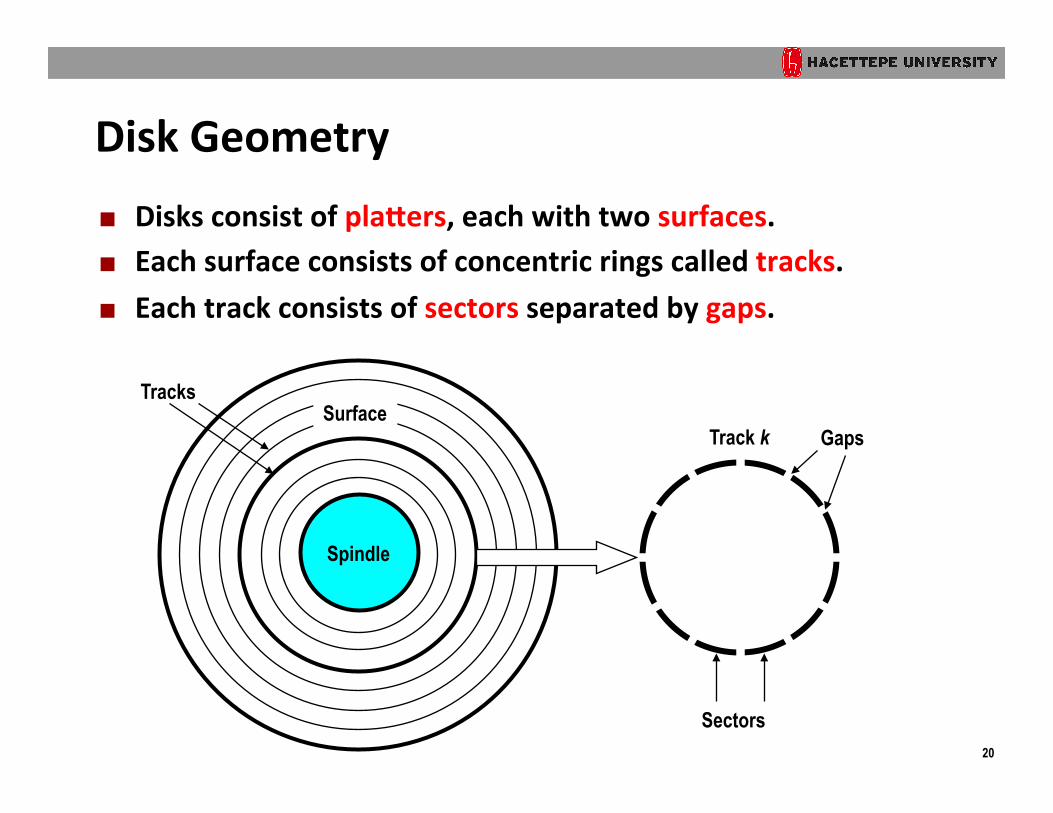
Disk Geometry ¢  Disks consist of plaVers, each with two surfaces. ¢  Each surface consists of concentric rings called tracks. ¢  Each track consists of sectors separated by gaps.

Spindle

Surface Tracks

Track k

Sectors

Gaps

21

Disk Geometry (Muliple-‐PlaVer View) ¢  Aligned tracks form a cylinder.

Surface 0 Surface 1 Surface 2 Surface 3 Surface 4 Surface 5

Cylinder k

Spindle

Platter 0

Platter 1

Platter 2

22

Disk Capacity ¢  Capacity: maximum number of bits that can be stored.

§  Vendors express capacity in units of gigabytes (GB), where 1 GB = 109 Bytes (Lawsuit pending! Claims decepOve adverOsing).

¢  Capacity is determined by these technology factors: §  Recording density (bits/in): number of bits that can be squeezed

into a 1 inch segment of a track. §  Track density (tracks/in): number of tracks that can be squeezed

into a 1 inch radial segment. §  Areal density (bits/in2): product of recording and track density.

¢  Modern disks par??on tracks into disjoint subsets called recording zones §  Each track in a zone has the same number of sectors, determined

by the circumference of innermost track. §  Each zone has a different number of sectors/track

23

Compu?ng Disk Capacity Capacity = (# bytes/sector) x (avg. # sectors/track) x

(# tracks/surface) x (# surfaces/plaVer) x (# plaVers/disk) Example:

§  512 bytes/sector §  300 sectors/track (on average) §  20,000 tracks/surface §  2 surfaces/plaker §  5 plakers/disk

Capacity = 512 x 300 x 20000 x 2 x 5 = 30,720,000,000

= 30.72 GB

24

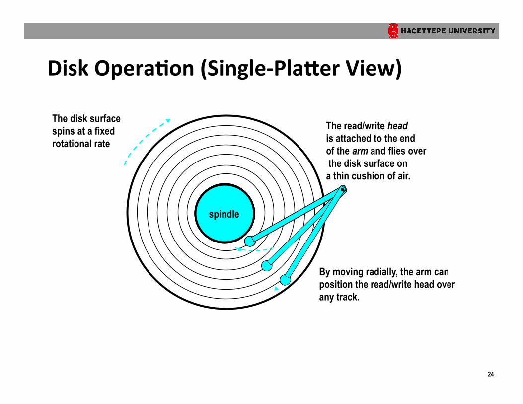
Disk Opera?on (Single-‐PlaVer View)

The disk surface spins at a fixed rotational rate

By moving radially, the arm can position the read/write head over any track.

The read/write head is attached to the end of the arm and flies over the disk surface on a thin cushion of air.

spindle

spindle

spin

dle

spindle spindle

25

Disk Opera?on (Mul?-‐PlaVer View)

Arm

Read/write heads move in unison

from cylinder to cylinder

Spindle

26

Tracks divided into sectors

Disk Structure -‐ top view of single plaVer

Surface organized into tracks

27

Disk Access

Head in position above a track

28

Disk Access

Rotation is counter-clockwise

29

Disk Access – Read

About to read blue sector

30


After BLUE read

After reading blue sector

31


After BLUE read

Red request scheduled next

32

Disk Access – Seek

After BLUE read Seek for RED

Seek to red’s track

33

Disk Access – Rota?onal Latency

After BLUE read Seek for RED Rotational latency

Wait for red sector to rotate around

34


After BLUE read Seek for RED Rotational latency After RED read

Complete read of red

35

Disk Access – Service Time Components

After BLUE read Seek for RED Rotational latency After RED read

Data transfer Seek Rota?onal latency

Data transfer

36

Disk Access Time ¢  Average ?me to access some target sector approximated by :

§  Taccess = Tavg seek + Tavg rotaOon + Tavg transfer ¢  Seek ?me (Tavg seek)

§  Time to posiOon heads over cylinder containing target sector. §  Typical Tavg seek is 3—9 ms

¢  Rota?onal latency (Tavg rota?on) §  Time waiOng for first bit of target sector to pass under r/w head. §  Tavg rotaOon = 1/2 x 1/RPMs x 60 sec/1 min §  Typical Tavg rotaOon = 7200 RPMs

¢  Transfer ?me (Tavg transfer) §  Time to read the bits in the target sector. §  Tavg transfer = 1/RPM x 1/(avg # sectors/track) x 60 secs/1 min.

37

Disk Access Time Example ¢  Given:

§  RotaOonal rate = 7,200 RPM §  Average seek Ome = 9 ms. §  Avg # sectors/track = 400.

¢  Derived: §  Tavg rotaOon = 1/2 x (60 secs/7200 RPM) x 1000 ms/sec = 4 ms. §  Tavg transfer = 60/7200 RPM x 1/400 secs/track x 1000 ms/sec = 0.02 ms §  Taccess = 9 ms + 4 ms + 0.02 ms

¢  Important points: §  Access Ome dominated by seek Ome and rotaOonal latency. §  First bit in a sector is the most expensive, the rest are free. §  SRAM access Ome is about 4 ns/doubleword, DRAM about 60 ns

§  Disk is about 40,000 Omes slower than SRAM, §  2,500 Omes slower then DRAM.

38

Logical Disk Blocks ¢  Modern disks present a simpler abstract view of the

complex sector geometry: §  The set of available sectors is modeled as a sequence of b-‐sized

logical blocks (0, 1, 2, ...)

¢  Mapping between logical blocks and actual (physical) sectors §  Maintained by hardware/firmware device called disk controller. §  Converts requests for logical blocks into (surface,track,sector)

triples.

¢  Allows controller to set aside spare cylinders for each zone. §  Accounts for the difference in “formaked capacity” and “maximum

capacity”.

39

I/O Bus

Main memory


ALU

Register file

CPU chip


Disk controller

Graphics adapter

USB controller

Mouse Keyboard Monitor Disk

I/O bus Expansion slots for other devices such as network adapters.

40

Reading a Disk Sector (1)

Main memory

ALU

Register file

CPU chip

Disk controller

Graphics adapter

USB controller

mouse keyboard Monitor Disk

I/O bus

Bus interface

CPU initiates a disk read by writing a command, logical block number, and destination memory address to a port (address) associated with disk controller.

41


Main memory

ALU

Register file

CPU chip

Disk controller

Graphics adapter

USB controller


I/O bus

Bus interface

Disk controller reads the sector and performs a direct memory access (DMA) transfer into main memory.

42


Main memory

ALU

Register file

CPU chip

Disk controller

Graphics adapter

USB controller


I/O bus

Bus interface

When the DMA transfer completes, the disk controller notifies the CPU with an interrupt (i.e., asserts a special “interrupt” pin on the CPU)

43

Solid State Disks (SSDs)

¢  Pages: 512KB to 4KB, Blocks: 32 to 128 pages ¢  Data read/wriVen in units of pages. ¢  Page can be wriVen only aier its block has been erased ¢  A block wears out aier 100,000 repeated writes.

Flash translation layer

I/O bus

Page 0 Page 1 Page P-1 … Block 0

… Page 0 Page 1 Page P-1 … Block B-1

Flash memory

Solid State Disk (SSD) Requests to read and write logical disk blocks

44

SSD Performance Characteris?cs

¢  Why are random writes so slow? §  Erasing a block is slow (around 1 ms) §  Write to a page triggers a copy of all useful pages in the block

§  Find an used block (new block) and erase it §  Write the page into the new block §  Copy other pages from old block to the new block

Sequen?al read tput 250 MB/s Sequen?al write tput 170 MB/s Random read tput 140 MB/s Random write tput 14 MB/s Rand read access 30 us Random write access 300 us

45

SSD Tradeoffs vs Rota?ng Disks ¢  Advantages

§  No moving parts à faster, less power, more rugged

¢  Disadvantages §  Have the potenOal to wear out

§  MiOgated by “wear leveling logic” in flash translaOon layer §  E.g. Intel X25 guarantees 1 petabyte (1015 bytes) of random writes before they wear out

§  In 2010, about 100 Omes more expensive per byte

¢  Applica?ons §  MP3 players, smart phones, laptops §  Beginning to appear in desktops and servers

46

Metric 1980 1985 1990 1995 2000 2005 2010 2010:1980 $/MB 8,000 880 100 30 1 0.1 0.06 130,000 access (ns) 375 200 100 70 60 50 40 9 typical size (MB) 0.064 0.256 4 16 64 2,000 8,000 125,000

Storage Trends

DRAM

SRAM

Metric 1980 1985 1990 1995 2000 2005 2010 2010:1980 $/MB 500 100 8 0.30 0.01 0.005 0.0003 1,600,000 access (ms) 87 75 28 10 8 4 3 29 typical size (MB) 1 10 160 1,000 20,000 160,000 1,500,000 1,500,000

Disk

Metric 1980 1985 1990 1995 2000 2005 2010 2010:1980 $/MB 19,200 2,900 320 256 100 75 60 320 access (ns) 300 150 35 15 3 2 1.5 200

47

CPU Clock Rates

1980 1990 1995 2000 2003 2005 2010 2010:1980 CPU 8080 386 Pentium P-III P-4 Core 2 Core i7 --- Clock rate (MHz) 1 20 150 600 3300 2000 2500 2500 Cycle time (ns) 1000 50 6 1.6 0.3 0.50 0.4 2500 Cores 1 1 1 1 1 2 4 4 Effective cycle 1000 50 6 1.6 0.3 0.25 0.1 10,000 time (ns)

Inflec?on point in computer history when designers hit the “Power Wall”

48

The CPU-‐Memory Gap The gap between DRAM, disk, and CPU speeds.

0.0

0.1

1.0

10.0

100.0

1,000.0

10,000.0

100,000.0

1,000,000.0

10,000,000.0

100,000,000.0

1980 1985 1990 1995 2000 2003 2005 2010

ns

Year

Disk seek time Flash SSD access time DRAM access time SRAM access time CPU cycle time Effective CPU cycle time

Disk

DRAM

CPU

SSD

49

Locality to the Rescue!

The key to bridging this CPU-‐Memory gap is a fundamental property of computer programs known as locality

50



51

Locality ¢  Principle of Locality: Programs tend to use data and

instruc?ons with addresses near or equal to those they have used recently

¢  Temporal locality: §  Recently referenced items are likely

to be referenced again in the near future

¢  Spa?al locality: §  Items with nearby addresses tend

to be referenced close together in Ome

52

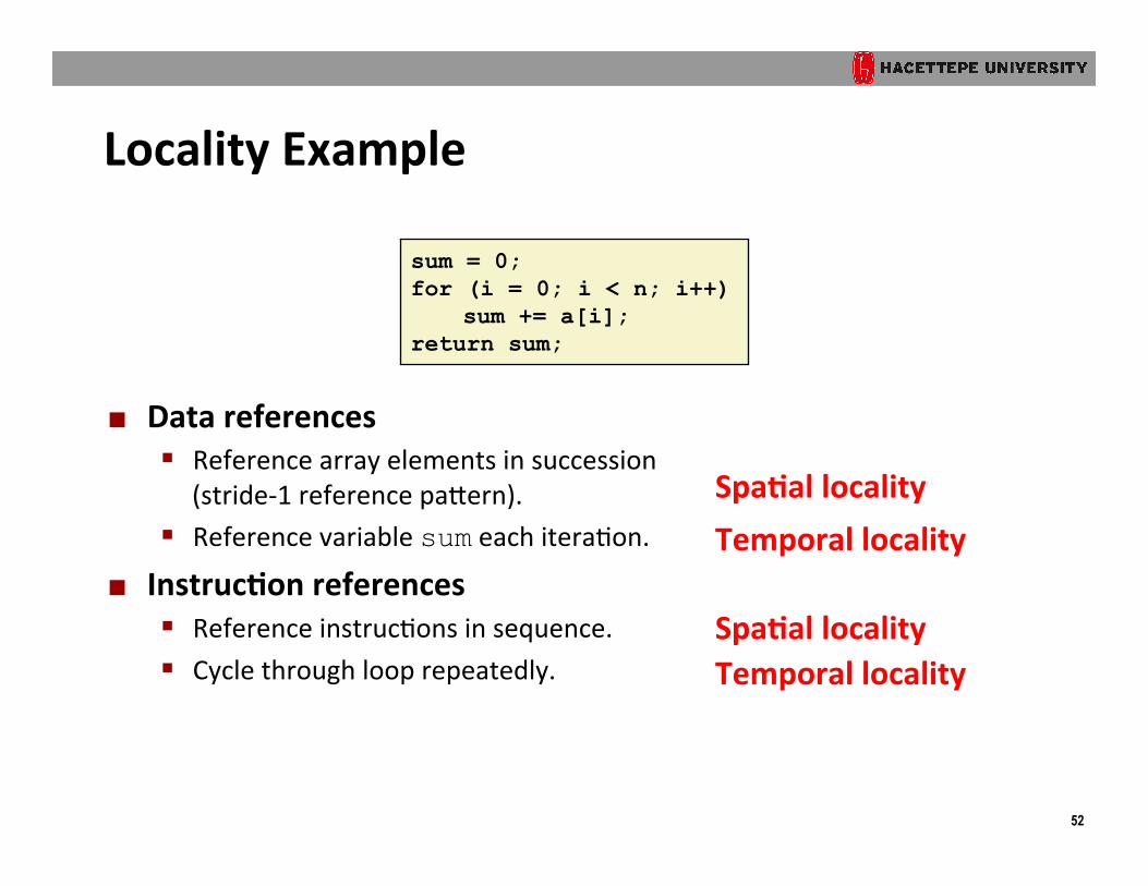
Locality Example

¢  Data references §  Reference array elements in succession

(stride-‐1 reference pakern). §  Reference variable sum each iteraOon.

¢  Instruc?on references §  Reference instrucOons in sequence. §  Cycle through loop repeatedly.

sum = 0; for (i = 0; i < n; i++)

sum += a[i]; return sum;

Spa?al locality Temporal locality

Spa?al locality Temporal locality

53

Qualita?ve Es?mates of Locality ¢  Claim: Being able to look at code and get a qualita?ve

sense of its locality is a key skill for a professional programmer.

¢  Ques?on: Does this func?on have good locality with respect to array a?

int sum_array_rows(int a[M][N]) { int i, j, sum = 0; for (i = 0; i < M; i++) for (j = 0; j < N; j++) sum += a[i][j]; return sum; }

54

Locality Example ¢  Ques?on: Does this func?on have good locality with

respect to array a?

int sum_array_cols(int a[M][N]) { int i, j, sum = 0; for (j = 0; j < N; j++) for (i = 0; i < M; i++) sum += a[i][j]; return sum; }

55

Locality Example ¢  Ques?on: Can you permute the loops so that the func?on

scans the 3-‐d array a with a stride-‐1 reference paVern (and thus has good spa?al locality)?

int sum_array_3d(int a[M][N][N]) { int i, j, k, sum = 0; for (i = 0; i < N; i++) for (j = 0; j < N; j++) for (k = 0; k < M; k++) sum += a[k][i][j]; return sum; }

56

Memory Hierarchies ¢  Some fundamental and enduring proper?es of hardware

and soiware: §  Fast storage technologies cost more per byte, have less capacity,

and require more power (heat!). §  The gap between CPU and main memory speed is widening. §  Well-‐wriken programs tend to exhibit good locality.

¢  These fundamental proper?es complement each other beau?fully.

¢  They suggest an approach for organizing memory and storage systems known as a memory hierarchy.

57



58

An Example Memory Hierarchy

Registers

L1 cache (SRAM)

Main memory (DRAM)

Local secondary storage (local disks)

Larger, slower, cheaper per byte

Remote secondary storage (tapes, distributed file systems, Web servers)

Local disks hold files retrieved from disks on remote network servers

Main memory holds disk blocks retrieved from local disks

L2 cache (SRAM)

L1 cache holds cache lines retrieved from L2 cache

CPU registers hold words retrieved from L1 cache

L2 cache holds cache lines retrieved from main memory

L0:

L1:

L2:

L3:

L4:

L5:

Smaller, faster, costlier per byte

59

Caches ¢  Cache: A smaller, faster storage device that acts as a staging

area for a subset of the data in a larger, slower device. ¢  Fundamental idea of a memory hierarchy:

§  For each k, the faster, smaller device at level k serves as a cache for the larger, slower device at level k+1.

¢  Why do memory hierarchies work? §  Because of locality, programs tend to access the data at level k more

oeen than they access the data at level k+1. §  Thus, the storage at level k+1 can be slower, and thus larger and

cheaper per bit.

¢  Big Idea: The memory hierarchy creates a large pool of storage that costs as much as the cheap storage near the boVom, but that serves data to programs at the rate of the fast storage near the top.

60

General Cache Concepts

0 1 2 3

4 5 6 7

8 9 10 11

12 13 14 15

8 9 14 3 Cache

Memory Larger, slower, cheaper memory viewed as par??oned into “blocks”

Data is copied in block-‐sized transfer units

Smaller, faster, more expensive memory caches a subset of the blocks

4

4

4

10

10

10

61

General Cache Concepts: Hit

0 1 2 3

4 5 6 7

8 9 10 11

12 13 14 15

8 9 14 3 Cache

Memory

Data in block b is needed Request: 14

14 Block b is in cache: Hit!

62

General Cache Concepts: Miss

0 1 2 3

4 5 6 7

8 9 10 11

12 13 14 15

8 9 14 3 Cache

Memory

Data in block b is needed Request: 12

Block b is not in cache: Miss!

Block b is fetched from memory Request: 12

12

12

12

Block b is stored in cache • Placement policy: determines where b goes

• Replacement policy: determines which block gets evicted (vicOm)

63

General Caching Concepts: Types of Cache Misses

¢  Cold (compulsory) miss §  Cold misses occur because the cache is empty.

¢  Conflict miss §  Most caches limit blocks at level k+1 to a small subset (someOmes a

singleton) of the block posiOons at level k. §  E.g. Block i at level k+1 must be placed in block (i mod 4) at level k.

§  Conflict misses occur when the level k cache is large enough, but mulOple data objects all map to the same level k block. §  E.g. Referencing blocks 0, 8, 0, 8, 0, 8, ... would miss every Ome.

¢  Capacity miss §  Occurs when the set of acOve cache blocks (working set) is larger than

the cache.

64

Examples of Caching in the Hierarchy

Hardware 0 On-‐Chip TLB Address transla?ons TLB

Web browser 10,000,000 Local disk Web pages Browser cache

Web cache

Network buffer cache

Buffer cache

Virtual Memory

L2 cache

L1 cache

Registers

Cache Type

Web pages

Parts of files

Parts of files

4-‐KB page

64-‐bytes block

64-‐bytes block

4-‐8 bytes words

What is Cached?

Web proxy server

1,000,000,000 Remote server disks

OS 100 Main memory

Hardware 1 On-‐Chip L1

Hardware 10 On/Off-‐Chip L2

AFS/NFS client 10,000,000 Local disk

Hardware + OS 100 Main memory

Compiler 0 CPU core

Managed By Latency (cycles) Where is it Cached?

Disk cache Disk sectors Disk controller 100,000 Disk firmware

65

Summary ¢  The speed gap between CPU, memory and mass storage

con?nues to widen.

¢  Well-‐wriVen programs exhibit a property called locality.

¢  Memory hierarchies based on caching close the gap by exploi?ng locality.

66



67

Cache Memories ¢  Cache memories are small, fast SRAM-‐based memories

managed automa?cally in hardware. §  Hold frequently accessed blocks of main memory

¢  CPU looks first for data in caches (e.g., L1, L2, and L3), then in main memory.

¢  Typical system structure:

Main memory


ALU

Register file CPU chip


Cache memories

68

General Cache Organiza?on (S, E, B) E = 2e lines per set

S = 2s sets

set

line

0 1 2 B-‐1 tag v

B = 2b bytes per cache block (the data)

Cache size: C = S x E x B data bytes

valid bit

69

Cache Read E = 2e lines per set

S = 2s sets

0 1 2 B-‐1 tag v

valid bit B = 2b bytes per cache block (the data)

t bits s bits b bits Address of word:

tag set index

block offset

data begins at this offset

• Locate set • Check if any line in set has matching tag

• Yes + line valid: hit • Locate data starEng at offset

70

Example: Direct Mapped Cache (E = 1)

S = 2s sets

Direct mapped: One line per set Assume: cache block size 8 bytes

t bits 0…01 100 Address of int:

0 1 2 7 tag v 3 6 5 4

0 1 2 7 tag v 3 6 5 4

0 1 2 7 tag v 3 6 5 4

0 1 2 7 tag v 3 6 5 4

find set

71

Example: Direct Mapped Cache (E = 1) Direct mapped: One line per set Assume: cache block size 8 bytes


0 1 2 7 tag v 3 6 5 4

match: assume yes = hit valid? +

block offset

tag

72

Example: Direct Mapped Cache (E = 1) Direct mapped: One line per set Assume: cache block size 8 bytes


0 1 2 7 tag v 3 6 5 4

match: assume yes = hit valid? +

int (4 Bytes) is here

block offset

No match: old line is evicted and replaced

73

Direct-‐Mapped Cache Simula?on M=16 byte addresses, B=2 bytes/block, S=4 sets, E=1 Blocks/set Address trace (reads, one byte per read):

0 [00002], 1 [00012], 7 [01112], 8 [10002], 0 [00002]

x t=1 s=2 b=1

xx x

0 ? ? v Tag Block

miss

1 0 M[0-‐1]

hit miss

1 0 M[6-‐7]

miss

1 1 M[8-‐9]

miss

1 0 M[0-‐1] Set 0 Set 1 Set 2 Set 3

Conflict miss!

74

A Higher Level Example int sum_array_rows(double a[16][16]) { int i, j; double sum = 0; for (i = 0; i < 16; i++) for (j = 0; j < 16; j++) sum += a[i][j]; return sum; }

32 B = 4 doubles

assume: cold (empty) cache, a[0][0] goes here

int sum_array_cols(double a[16][16]) { int i, j; double sum = 0; for (j = 0; i < 16; i++) for (i = 0; j < 16; j++) sum += a[i][j]; return sum; }

Ignore the variables sum, i, j

75

E-‐way Set Associa?ve Cache (Here: E = 2) E = 2: Two lines per set Assume: cache block size 8 bytes

t bits 0…01 100 Address of short int:

0 1 2 7 tag v 3 6 5 4 0 1 2 7 tag v 3 6 5 4

0 1 2 7 tag v 3 6 5 4 0 1 2 7 tag v 3 6 5 4

0 1 2 7 tag v 3 6 5 4 0 1 2 7 tag v 3 6 5 4

0 1 2 7 tag v 3 6 5 4 0 1 2 7 tag v 3 6 5 4

find set

76



0 1 2 7 tag v 3 6 5 4 0 1 2 7 tag v 3 6 5 4

compare both

valid? + match: yes = hit

block offset

tag

77



0 1 2 7 tag v 3 6 5 4 0 1 2 7 tag v 3 6 5 4

compare both

valid? + match: yes = hit

block offset

short int (2 Bytes) is here

No match: •  One line in set is selected for evic?on and replacement •  Replacement policies: random, least recently used (LRU), …

78

2-‐Way Set Associa?ve Cache Simula?on

M=16 byte addresses, B=2 bytes/block, S=2 sets, E=2 blocks/set Address trace (reads, one byte per read):

0 [00002], 1 [00012], 7 [01112], 8 [10002], 0 [00002]

xx t=2 s=1 b=1

x x

0 ? ? v Tag Block

0

0 0

miss

1 00 M[0-‐1]

hit miss

1 01 M[6-‐7]

miss

1 10 M[8-‐9]

hit

Set 0

Set 1

79

A Higher Level Example int sum_array_rows(double a[16][16]) { int i, j; double sum = 0; for (i = 0; i < 16; i++) for (j = 0; j < 16; j++) sum += a[i][j]; return sum; }

32 B = 4 doubles

assume: cold (empty) cache, a[0][0] goes here

int sum_array_rows(double a[16][16]) { int i, j; double sum = 0; for (j = 0; i < 16; i++) for (i = 0; j < 16; j++) sum += a[i][j]; return sum; }

Ignore the variables sum, i, j

80

What about writes? ¢  Mul?ple copies of data exist:

§  L1, L2, Main Memory, Disk

¢  What to do on a write-‐hit? §  Write-‐through (write immediately to memory) §  Write-‐back (defer write to memory unOl replacement of line)

§  Need a dirty bit (line different from memory or not)

¢  What to do on a write-‐miss? §  Write-‐allocate (load into cache, update line in cache)

§  Good if more writes to the locaOon follow §  No-‐write-‐allocate (writes immediately to memory)

¢  Typical §  Write-‐through + No-‐write-‐allocate §  Write-‐back + Write-‐allocate

81

Intel Core i7 Cache Hierarchy

Regs

L1 d-cache

L1 i-cache

L2 unified cache

Core 0

Regs

L1 d-cache

L1 i-cache

L2 unified cache

Core 3

…

L3 unified cache (shared by all cores)

Main memory

Processor package L1 i-‐cache and d-‐cache:

32 KB, 8-‐way, Access: 4 cycles

L2 unified cache:

256 KB, 8-‐way, Access: 11 cycles

L3 unified cache: 8 MB, 16-‐way, Access: 30-‐40 cycles

Block size: 64 bytes for all caches.

82

Cache Performance Metrics ¢  Miss Rate

§  FracOon of memory references not found in cache (misses / accesses) = 1 – hit rate

§  Typical numbers (in percentages): §  3-‐10% for L1 §  can be quite small (e.g., < 1%) for L2, depending on size, etc.

¢  Hit Time §  Time to deliver a line in the cache to the processor

§  includes Ome to determine whether the line is in the cache §  Typical numbers:

§  1-‐2 clock cycle for L1 §  5-‐20 clock cycles for L2

¢  Miss Penalty §  AddiOonal Ome required because of a miss

§  typically 50-‐200 cycles for main memory (Trend: increasing!)

83

Lets think about those numbers ¢  Huge difference between a hit and a miss

§  Could be 100x, if just L1 and main memory

¢  Would you believe 99% hits is twice as good as 97%? §  Consider:

cache hit Ome of 1 cycle miss penalty of 100 cycles

§  Average access Ome: 97% hits: 1 cycle + 0.03 * 100 cycles = 4 cycles 99% hits: 1 cycle + 0.01 * 100 cycles = 2 cycles

¢  This is why “miss rate” is used instead of “hit rate”

84

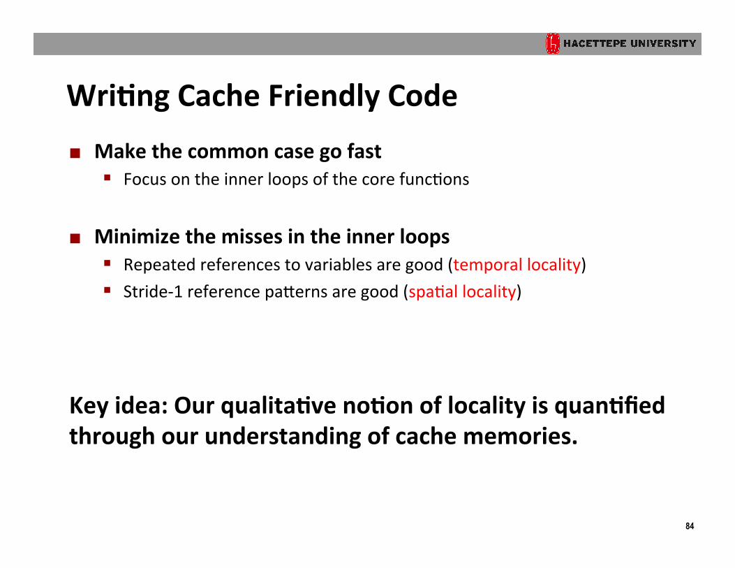
Wri?ng Cache Friendly Code ¢  Make the common case go fast

§  Focus on the inner loops of the core funcOons

¢  Minimize the misses in the inner loops §  Repeated references to variables are good (temporal locality) §  Stride-‐1 reference pakerns are good (spaOal locality)

Key idea: Our qualita?ve no?on of locality is quan?fied through our understanding of cache memories.

85

Today ¢  Storage technologies and trends ¢  Locality of reference ¢  Caching in the memory hierarchy ¢  Cache organiza?on and opera?on ¢  Performance impact of caches


86

The Memory Mountain ¢  Read throughput (read bandwidth)

§  Number of bytes read from memory per second (MB/s)

¢  Memory mountain: Measured read throughput as a

func?on of spa?al and temporal locality. §  Compact way to characterize memory system performance.

87

Memory Mountain Test Func?on /* The test function */ void test(int elems, int stride) { int i, result = 0; volatile int sink; for (i = 0; i < elems; i += stride)

result += data[i]; sink = result; /* So compiler doesn't optimize away the loop */ } /* Run test(elems, stride) and return read throughput (MB/s) */ double run(int size, int stride, double Mhz) { double cycles; int elems = size / sizeof(int); test(elems, stride); /* warm up the cache */ cycles = fcyc2(test, elems, stride, 0); /* call test(elems,stride) */ return (size / stride) / (cycles / Mhz); /* convert cycles to MB/s */ }

88

The Memory Mountain

64M

8M 1M

128K

16K

2K 0

1000

2000

3000

4000

5000

6000

7000 s1

s3

s5

s7

s9

s1

1 s1

3 s1

5 s3

2 Working set size (bytes)

Rea

d th

roug

hput

(MB

/s)

Stride (x8 bytes)

Intel Core i7 32 KB L1 i-‐cache 32 KB L1 d-‐cache 256 KB unified L2 cache 8M unified L3 cache All caches on-‐chip

89

The Memory Mountain

64M

8M 1M

128K

16K

2K 0

1000

2000

3000

4000

5000

6000

7000 s1

s3

s5

s7

s9

s1

1 s1

3 s1

5 s3


Rea

d th

roug

hput

(MB

/s)

Stride (x8 bytes)


Slopes of spaEal locality

90

The Memory Mountain

64M

8M 1M

128K

16K

2K 0

1000

2000

3000

4000

5000

6000

7000 s1

s3

s5

s7

s9

s1

1 s1

3 s1

5 s3


Rea

d th

roug

hput

(MB

/s)

Stride (x8 bytes)

L1"

L2"

Mem"

L3"


Slopes of spaEal locality

Ridges of Temporal locality

91



92

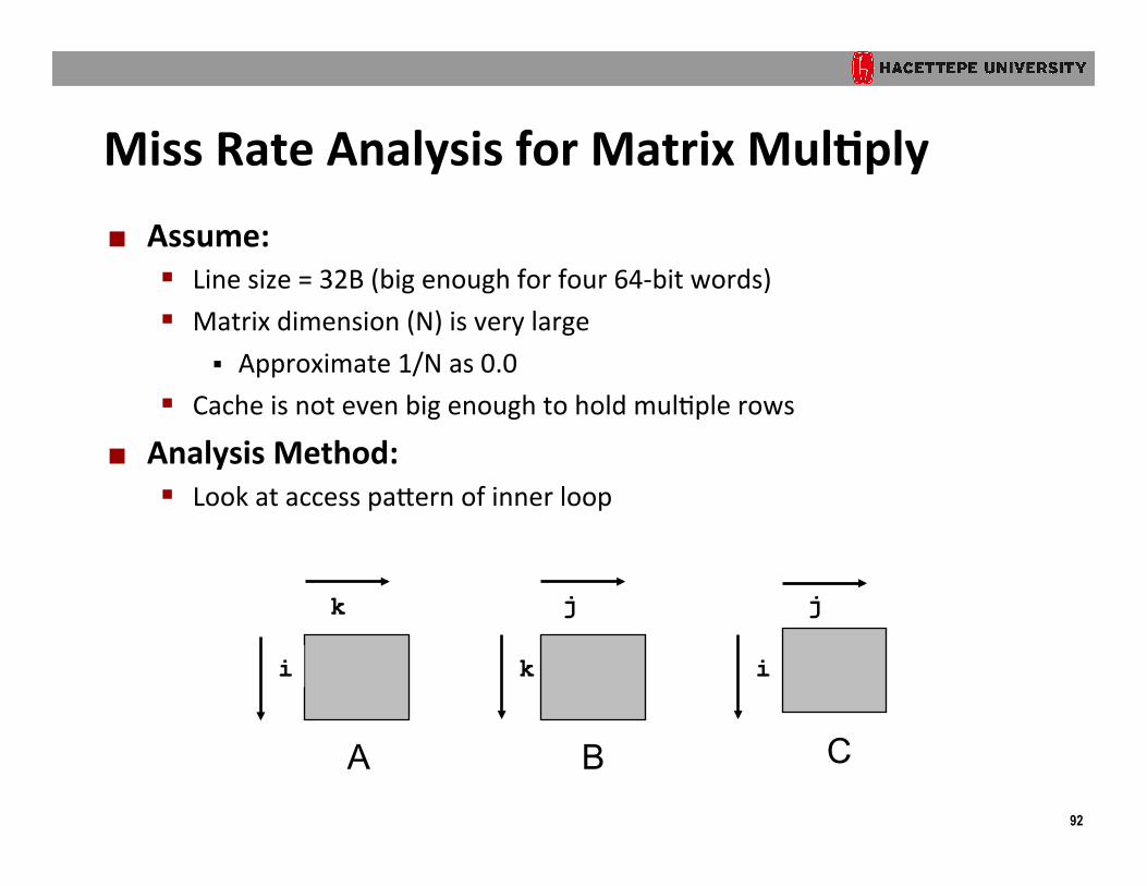
Miss Rate Analysis for Matrix Mul?ply ¢  Assume:

§  Line size = 32B (big enough for four 64-‐bit words) §  Matrix dimension (N) is very large

§  Approximate 1/N as 0.0 §  Cache is not even big enough to hold mulOple rows

¢  Analysis Method: §  Look at access pakern of inner loop

A

k

i

B

k

j

C

i

j

93

Matrix Mul?plica?on Example ¢  Descrip?on:

§  MulOply N x N matrices §  O(N3) total operaOons §  N reads per source

element §  N values summed per

desOnaOon §  but may be able to hold in register

/* ijk */ for (i=0; i<n; i++) { for (j=0; j<n; j++) { sum = 0.0; for (k=0; k<n; k++) sum += a[i][k] * b[k][j]; c[i][j] = sum; } }

Variable sum held in register

94

Layout of C Arrays in Memory (review) ¢  C arrays allocated in row-‐major order

§  each row in conOguous memory locaOons ¢  Stepping through columns in one row:

§  for (i = 0; i < N; i++) sum += a[0][i];

§  accesses successive elements §  if block size (B) > 4 bytes, exploit spaOal locality

§  compulsory miss rate = 4 bytes / B ¢  Stepping through rows in one column:

§  for (i = 0; i < n; i++) sum += a[i][0];

§  accesses distant elements §  no spaOal locality!

§  compulsory miss rate = 1 (i.e. 100%)

95

Matrix Mul?plica?on (ijk)

/* ijk */ for (i=0; i<n; i++) { for (j=0; j<n; j++) { sum = 0.0; for (k=0; k<n; k++) sum += a[i][k] * b[k][j]; c[i][j] = sum; } }

A B C (i,*)

(*,j) (i,j)

Inner loop:

Column-‐ wise

Row-‐wise Fixed

Misses per inner loop iteraOon: A B C 0.25 1.0 0.0

96

Matrix Mul?plica?on (jik)

/* jik */ for (j=0; j<n; j++) { for (i=0; i<n; i++) { sum = 0.0; for (k=0; k<n; k++) sum += a[i][k] * b[k][j]; c[i][j] = sum } }

A B C (i,*)

(*,j) (i,j)

Inner loop:

Row-‐wise Column-‐ wise

Fixed


97

Matrix Mul?plica?on (kij)

/* kij */ for (k=0; k<n; k++) { for (i=0; i<n; i++) { r = a[i][k]; for (j=0; j<n; j++) c[i][j] += r * b[k][j]; } }

A B C (i,*)

(i,k) (k,*)

Inner loop:

Row-‐wise Row-‐wise Fixed


98

Matrix Mul?plica?on (ikj)

/* ikj */ for (i=0; i<n; i++) { for (k=0; k<n; k++) { r = a[i][k]; for (j=0; j<n; j++) c[i][j] += r * b[k][j]; } }

A B C (i,*)

(i,k) (k,*)

Inner loop:

Row-‐wise Row-‐wise Fixed


99

Matrix Mul?plica?on (jki)

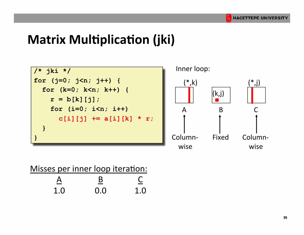
/* jki */ for (j=0; j<n; j++) { for (k=0; k<n; k++) { r = b[k][j]; for (i=0; i<n; i++) c[i][j] += a[i][k] * r; } }

A B C

(*,j) (k,j)

Inner loop:

(*,k)

Column-‐ wise

Column-‐ wise

Fixed


100

Matrix Mul?plica?on (kji)

/* kji */ for (k=0; k<n; k++) { for (j=0; j<n; j++) { r = b[k][j]; for (i=0; i<n; i++) c[i][j] += a[i][k] * r; } }

A B C

(*,j) (k,j)

Inner loop:

(*,k)

Fixed Column-‐ wise

Column-‐ wise


101

Summary of Matrix Mul?plica?on

ijk (& jik): •  2 loads, 0 stores •  misses/iter = 1.25

kij (& ikj): •  2 loads, 1 store •  misses/iter = 0.5

jki (& kji): •  2 loads, 1 store •  misses/iter = 2.0

for (i=0; i<n; i++) { for (j=0; j<n; j++) { sum = 0.0;

for (k=0; k<n; k++) sum += a[i][k] * b[k][j]; c[i][j] = sum; } }

for (k=0; k<n; k++) { for (i=0; i<n; i++) { r = a[i][k];

for (j=0; j<n; j++) c[i][j] += r * b[k][j]; } }

for (j=0; j<n; j++) { for (k=0; k<n; k++) { r = b[k][j];

for (i=0; i<n; i++) c[i][j] += a[i][k] * r; } }

102

Core i7 Matrix Mul?ply Performance

0

10

20

30

40

50

60

50 100 150 200 250 300 350 400 450 500 550 600 650 700 750

Cyc

les

per i

nner

loop

iter

atio

n

Array size (n)

jki kji ijk jik kij ikj

jki / kji

ijk / jik

kij / ikj

103



104

Example: Matrix Mul?plica?on

a b

i

j

* c

=

c = (double *) calloc(sizeof(double), n*n); /* Multiply n x n matrices a and b */ void mmm(double *a, double *b, double *c, int n) { int i, j, k; for (i = 0; i < n; i++)

for (j = 0; j < n; j++) for (k = 0; k < n; k++)

c[i*n+j] += a[i*n + k]*b[k*n + j]; }

105

Cache Miss Analysis ¢  Assume:

§  Matrix elements are doubles §  Cache block = 8 doubles §  Cache size C << n (much smaller than n)

¢  First itera?on: §  n/8 + n = 9n/8 misses

§  Aeerwards in cache: (schemaOc)

* =

n

* = 8 wide

106


§  Matrix elements are doubles §  Cache block = 8 doubles §  Cache size C << n (much smaller than n)

¢  Second itera?on: §  Again:

n/8 + n = 9n/8 misses

¢  Total misses: §  9n/8 * n2 = (9/8) * n3

n

* = 8 wide

107

Blocked Matrix Mul?plica?on c = (double *) calloc(sizeof(double), n*n); /* Multiply n x n matrices a and b */ void mmm(double *a, double *b, double *c, int n) { int i, j, k; for (i = 0; i < n; i+=B)

for (j = 0; j < n; j+=B) for (k = 0; k < n; k+=B)

/* B x B mini matrix multiplications */ for (i1 = i; i1 < i+B; i++) for (j1 = j; j1 < j+B; j++) for (k1 = k; k1 < k+B; k++)

c[i1*n+j1] += a[i1*n + k1]*b[k1*n + j1]; }

a b

i1

j1

* c

= c

+

Block size B x B

2

2 A Blocked Version of Matrix Multiply

Blocking a matrix multiply routine works by partitioning the matrices into submatrices and then exploitingthe mathematical fact that these submatrices can be manipulated just like scalars. For example, suppose wewant to compute C = AB, where A, B, and C are each 8 ! 8 matrices. Then we can partition each matrixinto four 4 ! 4 submatrices:

!

C11 C12

C21 C22

"

=

!

A11 A12

A21 A22

" !

B11 B12

B21 B22

"

where

C11 = A11B11 + A12B21

C12 = A11B12 + A12B22

C21 = A21B11 + A22B21

C22 = A21B12 + A22B22

Figure 1 shows one version of blocked matrix multiplication, which we call the bijk version. The basicidea behind this code is to partition A and C into 1 ! bsize row slivers and to partition B into bsize! bsizeblocks. The innermost (j, k) loop pair multiplies a sliver of A by a block of B and accumulates the resultinto a sliver of C . The i loop iterates through n row slivers of A and C , using the same block in B.

Figure 2 gives a graphical interpretation of the blocked code from Figure 1. The key idea is that it loadsa block of B into the cache, uses it up, and then discards it. References to A enjoy good spatial localitybecause each sliver is accessed with a stride of 1. There is also good temporal locality because the entiresliver is referenced bsize times in succession. References to B enjoy good temporal locality because theentire bsize ! bsize block is accessed n times in succession. Finally, the references to C have good spatiallocality because each element of the sliver is written in succession. Notice that references to C do not havegood temporal locality because each sliver is only accessed one time.

Blocking can make code harder to read, but it can also pay big performance dividends. Figure 3 shows theperformance of two versions of blocked matrix multiply on a Pentium III Xeon system (bsize = 25). Noticethat blocking improves the running time by a factor of two over the best nonblocked version, from about20 cycles per iteration down to about 10 cycles per iteration. The other interesting thing about blockingis that the time per iteration remains nearly constant with increasing array size. For small array sizes, theadditional overhead in the blocked version causes it to run slower than the nonblocked versions. There is acrossover point at about n = 100, after which the blocked version runs faster.

We caution that blocking matrix multiply does not improve performance on all systems. For example, ona Core i7 system, there exist unblocked versions of matrix multiply that have the same performance as thebest blocked version.

2

2 A Blocked Version of Matrix Multiply

Blocking a matrix multiply routine works by partitioning the matrices into submatrices and then exploitingthe mathematical fact that these submatrices can be manipulated just like scalars. For example, suppose wewant to compute C = AB, where A, B, and C are each 8 ! 8 matrices. Then we can partition each matrixinto four 4 ! 4 submatrices:

!

C11 C12

C21 C22

"

=

!

A11 A12

A21 A22

" !

B11 B12

B21 B22

"

where

C11 = A11B11 + A12B21

C12 = A11B12 + A12B22

C21 = A21B11 + A22B21

C22 = A21B12 + A22B22

Figure 1 shows one version of blocked matrix multiplication, which we call the bijk version. The basicidea behind this code is to partition A and C into 1 ! bsize row slivers and to partition B into bsize! bsizeblocks. The innermost (j, k) loop pair multiplies a sliver of A by a block of B and accumulates the resultinto a sliver of C . The i loop iterates through n row slivers of A and C , using the same block in B.

Figure 2 gives a graphical interpretation of the blocked code from Figure 1. The key idea is that it loadsa block of B into the cache, uses it up, and then discards it. References to A enjoy good spatial localitybecause each sliver is accessed with a stride of 1. There is also good temporal locality because the entiresliver is referenced bsize times in succession. References to B enjoy good temporal locality because theentire bsize ! bsize block is accessed n times in succession. Finally, the references to C have good spatiallocality because each element of the sliver is written in succession. Notice that references to C do not havegood temporal locality because each sliver is only accessed one time.

Blocking can make code harder to read, but it can also pay big performance dividends. Figure 3 shows theperformance of two versions of blocked matrix multiply on a Pentium III Xeon system (bsize = 25). Noticethat blocking improves the running time by a factor of two over the best nonblocked version, from about20 cycles per iteration down to about 10 cycles per iteration. The other interesting thing about blockingis that the time per iteration remains nearly constant with increasing array size. For small array sizes, theadditional overhead in the blocked version causes it to run slower than the nonblocked versions. There is acrossover point at about n = 100, after which the blocked version runs faster.

We caution that blocking matrix multiply does not improve performance on all systems. For example, ona Core i7 system, there exist unblocked versions of matrix multiply that have the same performance as thebest blocked version.

108


§  Cache block = 8 doubles §  Cache size C << n (much smaller than n) §  Three blocks fit into cache: 3B2 < C

¢  First (block) itera?on: §  B2/8 misses for each block §  2n/B * B2/8 = nB/4

(omi}ng matrix c)

§  Aeerwards in cache (schemaOc)

* =

* =

Block size B x B

n/B blocks

109


§  Cache block = 8 doubles §  Cache size C << n (much smaller than n) §  Three blocks fit into cache: 3B2 < C

¢  Second (block) itera?on: §  Same as first iteraOon §  2n/B * B2/8 = nB/4

¢  Total misses: §  nB/4 * (n/B)2 = n3/(4B)

* =

Block size B x B

n/B blocks

110

Summary ¢  No blocking: (9/8) * n3

¢  Blocking: 1/(4B) * n3

¢  Suggest largest possible block size B, but limit 3B2 < C!

¢  Reason for drama?c difference: §  Matrix mulOplicaOon has inherent temporal locality:

§  Input data: 3n2, computaOon 2n3

§  Every array elements used O(n) Omes! §  But program has to be wriken properly

111

Concluding Observa?ons ¢  Programmer can op?mize for cache performance

§  How data structures are organized §  How data are accessed

§  Nested loop structure §  Blocking is a general technique

¢  All systems favor “cache friendly code” §  Ge}ng absolute opOmum performance is very pla~orm specific

§  Cache sizes, line sizes, associaOviOes, etc. §  Can get most of the advantage with generic code

§  Keep working set reasonably small (temporal locality) §  Use small strides (spaOal locality)

the$memory$hierarchy$ - hacettepe · 1 the$memory$hierarchy$ $ fall$2012$ instructors:$$...

Documents