1

Optimized Train Control

The William W. Hay Railroad Engineering Seminar Series

Grainger Engineering Library - 2nd Floor - Commons Room 233University of Illinois at Urbana-Champaign

April 3, 2009

David Thurston, FIRSE, P.E.

2

Introduction

Train Control has existed since the beginning of railways.

Safety has always been of the first importance in Signal Design.

Regardless of Train Control type, braking distance is a common element.

Understanding Braking distance is a key element in Capacity.

3

Rail Capacity

As miles of road continue to shrink, the traffic applied to the remaining lines is increasing.

Class 1 Freight Railroads Traffic vs. Track Miles

300

500

700

900

1100

1300

1500

1930

1935

1940

1945

1950

1955

1960

1965

1970

1975

1980

1985

1990

1995

2000

2005

Year

Gro

ss T

ons

Hau

led

(in th

ousa

nds)

90

110

130

150

170

190

210

230

Rou

te M

iles

(in th

ousa

nds)

Revunue Ton-Miles Road Miles Operated

4

Rail Capacity

The same traffic trend applies to rail and transit.

Transit Growth

7.5

8.0

8.5

9.0

9.5

10.0

10.5

11.0

1995 1996 1997 1998 1999 2000 2001 2002 2003 2004 2005 2006 2007 2008

Year

Bill

ions

of P

asse

nger

trip

s

5

Capacity Constraints

Safety is assured through adherence to the rules.

15th-16th Street Sta. 12th-13th Street Sta.

Terminal Station(end of line)

Switches toRoute trainsStation Platforms

Tracks

Over 1,500 feet

6

Capacity Constraints

There is a trade off between Capacity and Speed

Capacity for Various Speeds

35

40

45

50

55

60

65

30 60 80 90

Cab Signal Speed Command

Trai

ns p

er H

our

7

Contemporary Requirements

Designs are becoming more conservative.There is an increasing reliance on

Enforcement.Available (and soon to be available) technology

offers value added features:

• Heath Monitoring• Predictive Maintenance• TSR’s• RWP protection

An ACSES ADU

8

Train Control

• Manual Block (Time Table and Train Order) • Track Warrant Control (TWC or Form “D”)• Automatic Block Signals (including ABS, APB,

and CTC)• Trip Stop• Inductor based Automatic Train Stop• Cab Signals (With and without enforcement)• Profile Based Systems• Communications Based Train Control (CBTC

and PTC)

9

The Role of Train Control

• Traffic Flow• Remote Control• Movement Authority• Operational Safety

–Highway crossings–Interlocking

(Routing)–Train Separation

10

Train Separation

• Train Separation is directly related to Capacity

Braking Distance to Stop for Following Train

Minimum Headway is the Time Separation of Two Trains at their Closest Safe Braking Distance

Distance

Trai

n S

peed

11

Signal Spacing

Safety is assured through adherence to the rules.

(Green) (Green) (Green) (Green)

(Red) (Green) (Green) (Green)

(Yellow) (Red) (Green) (Green)

(Green) (Yellow) (Red) (Green)

Direction of Travel

Stopping Distance Stopping Distance

12

A Common Factor in Train Control

The capacity of different advanced train control systems such as Profile based Cab Signals or Communications Based Train Control is negligible (as shown in the example below).

The key factor throughout is the calculation of Safe Braking Distance.

13

SP

EE

D

SBD Stopping Curve

Performance Stopping Curve

Lost Capacity

DISTANCE

Resultant Capacity Gap

Conservative design generate lost capacity by stopping trains well short of required occupied blocks

14

Safe Braking Distance Model

• A mathematical expression of stopping distance

• Little uniformity in use or application

• IEEE Working Group 25 within the Standards Association was assigned the task of creating guidelines for SBD to address these issues

15

Safe Braking Distance Model

Current Progress:• Draft Guideline is complete• Initial Ballot complete with

comments• Response complete and all

comments addressed• Formal response or re-ballot in

progress

16

IEEE SBD Model (Draft)

TOTAL SBD

SP

EE

D

AOverspeed

B Entry Point C

FreeRunning

H + IMinimum Braking Rate and

Braking Rate Factors

DRunaway

Acceleration

EPropulsionRemoval

FDead Time

GBrake

Build up

JOverhang

DISTANCE

17

Conventional Model Example

A – Maximum Entry Speed: 50 mph plus 3 mph

B – Entry Point: (Initial measurement point)

C – Distance Traveled During Reaction Time:

Where:• DC = Reaction Distance component of SBD, • VA = Maximum Entry Speed, and• tR = Reaction Time.

RAC tVD *466.1*=

18

Conventional Model Example

D – Runaway Acceleration: 2.0 mphpsTherefore, the speed at the end of the

Runaway Acceleration period is 55 mph, and integrating over the one second period yields a distance traveled of

DD = 79.2 ft.E – Propulsion Removal: For this model we

assume Linear deceleration to zero over one second providing a distance of

DE = 81.4 ft

19

Conventional Model Example

F – Dead Time: Coasting after propulsion removal for one second

DF = 82.1 ft,G – Brake Build Up: 50% of full braking rate for

one second. DG = 81.8 ft.

H+I – Brake Rate: Where: DI+H = Brake rate component of SBD,

VI+H = Velocity at the beginning of the braking period

DH+I = 2,567 ft.J - Overhang: DJ = 15 ft.

8333.0*2HIHI VD ++ =

20

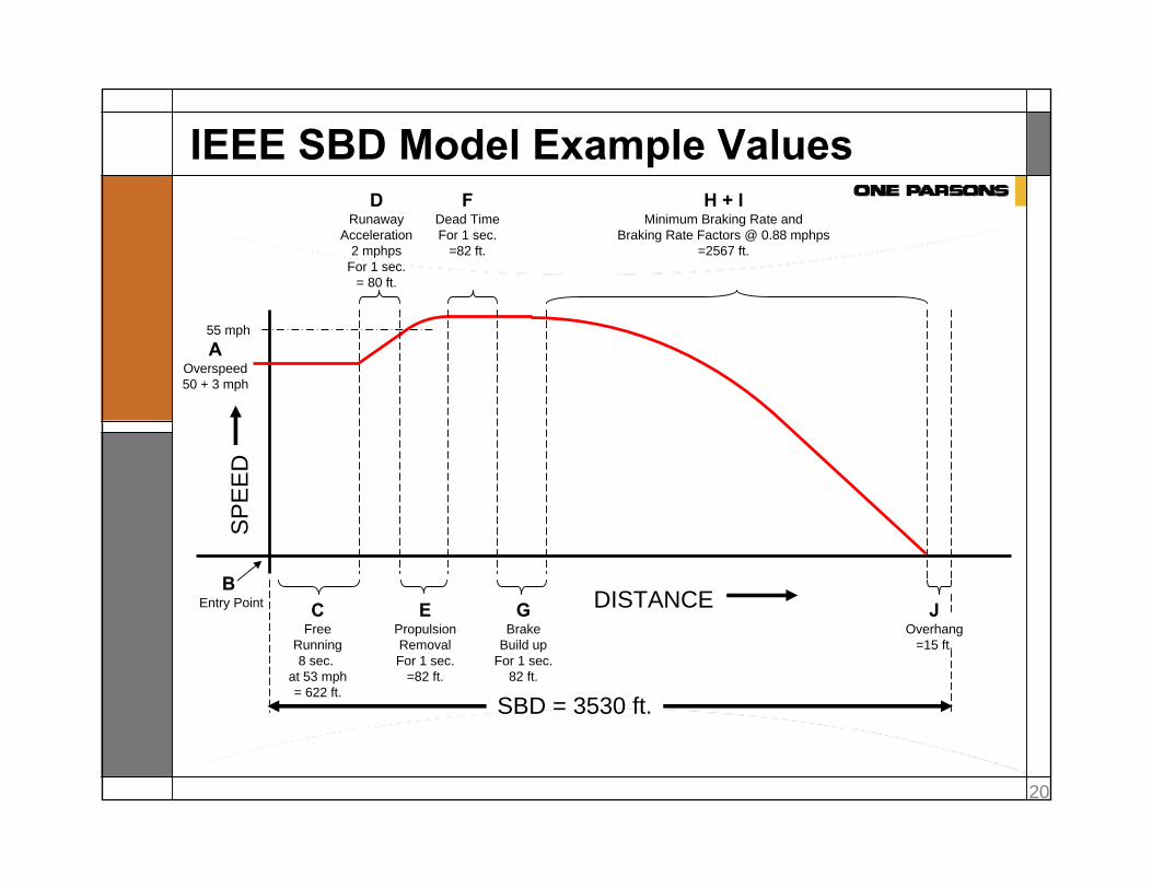
IEEE SBD Model Example Values

SP

EE

D

SBD = 3530 ft.

AOverspeed50 + 3 mph

B Entry Point C

FreeRunning8 sec.

at 53 mph= 622 ft.

H + IMinimum Braking Rate and

Braking Rate Factors @ 0.88 mphps=2567 ft.

DRunaway

Acceleration2 mphps

For 1 sec.= 80 ft.

EPropulsionRemovalFor 1 sec.

=82 ft.

FDead TimeFor 1 sec.

=82 ft.

GBrake

Build upFor 1 sec.

82 ft.

JOverhang

=15 ft.

55 mph

DISTANCE

21

Stochastic Approach

Origins of approach can be found in previous attempts to address capacity issues with the traditional methodologies

Traditional is Worst Case, but we don’t know “how safe” it is. Is there excess distance in traditional calculations?

The introduction of probability can help answer these questions.

22

Stochastic Approach

What is safe? We cancan determine a minimum SBD thru

the use of probability as the mean time between hazardous events.

One such metric was contained in a report to Congress in 1976 that stated the minimum acceptable rate of occurrence of fatalities on a transit property utilizing Automatic Train Protection was one in two billion passengers

23

Stochastic Approach

By estimating the train density, train carrying capacity, and number of brake applications required for operations for a given system, the probability for an overrun of the SBD that would cause a hazard for this level of safety can be determined.

Utilize the same IEEE Model to ensure uniformity of results

24

Stochastic ApproachFor Example:

LRT trains running 19 hours per day, Headway is 15 minutes

For a 15 mile system, lets say there are 10 stations protected by signals

End to end run time is approximately 30 minutes, forcing a brake application every 3 minutes

76 trains x 19 hours x 60 minutes/hour / 3 minutes between braking = 10.5 M brake applications/year

therefore the probability of stopping outside the provided distance is:

1/(10.5M*P(Stopping Distance>SBD)

25

Stochastic Approach

But what is safe?

Using the report to Congress, the mean time to fatal accident is:

(20B x Fatalities per accident)/passengers per year

# 0f passengers is: 76 trains x 150 people, 365 days = 4.2M

With a single fatality each year, the mean time to hazard is:

(20 x 1010 x 1)/ 4.2M) = 4762 years

26

Stochastic Approach

To compare this to the Probability of exceeding the provided distance,

P(D>SBD) = 1/(stops or reductions for per year)(Mean time between to hazard)

= 1/(10.5M)(4762) = 2 x 10-11

By calculating the Probability of the IEEE SBD model, for all available scenarios, the optimum SBD can be determined.

27

Stochastic Approach

Each part of the model is assumed to be independent, therefore distance contributed by each event is added while the probability of a hazardous event is multiplied

By plotting all possible combinations of results (probability of overrunning vs. braking distance), we can see if the traditional case is overly conservative.

28

Stochastic Approach

Each portion of the model can be represented as a Probability Distribution Function (PDF of CDF)

For Example, Overspeed can be represented thru empirical data as:

1 1 x ≥ 20.9 0.9 1 ≤ x < 20.8 0.8 -1 ≤ x < 10.7

0.6 F x (x) = P = (X(ξ) ≤ x) = 0.5

0.4 0.3 -2 ≤ x < -10.3

0.2 0.1 -3 ≤ x < -20.1 0 x < -3

-4 -3 -2 -1 0 0 1 2 3 4 Overspeed in mph

29

Stochastic Approach

Similar analysis can be performed for each model part where each portion of the PDF represents the probability of that portion of the SBD model exceeding the appropriate parameter

Every possible combination of every event is combined to provide a family of SBD and total probability

30

Stochastic Approach

By creating either a table or plot of the probabilities of exceeding the provided distance vs. the calculated distances, we can interpolate which of the solutions provides the minimum distance that provides the level of safety desired.

31

Stochastic Approach

Anticipated decrease in distance from the traditional to the stochastic method of calculating SBD is 10 to 20%.

This corresponds to an increase in system capacity

Further study is required to maximize a closed loop approach where by the actual brake rate (Part I and H of the IEEE model) is measured and is used to dynamically change the on board calculation of SBD for all trains running within the system

32

Thank you