arX

iv:1

410.

0536

v1 [

astr

o-ph

.GA

] 2

Oct

201

4Astronomy & Astrophysicsmanuscript no. 47˙T c© ESO 2014October 3, 2014

The white dwarf cooling sequence of 47 TucanaeEnrique Garcıa–Berro1,2, Santiago Torres1,2, Leandro G. Althaus3,4, and Marcelo M. Miller Bertolami4,5,6

1 Departament de Fısica Aplicada, Universitat Politecnica de Catalunya, c/Esteve Terrades 5, 08860 Castelldefels, Spain2 Institute for Space Studies of Catalonia, c/Gran Capita 2–4, Edif. Nexus 104, 08034 Barcelona, Spain3 Facultad de Ciencias Astronomicas y Geofısicas, Universidad Nacional de La Plata, Paseo del Bosque s/n, 1900 La Plata, Argentina4 Instituto de Astrofısica de La Plata, UNLP-CONICET, Paseodel Bosque s/n, 1900 La Plata, Argentina5 Max-Planck-Institut fur Astrophysik, Karl-Schwarzschild Strasse 1, 85748 Garching, Germany6 Post-doctoral Fellow of the Alexander von Humboldt Foundation

October 3, 2014

Abstract

Context. 47 Tucanae is one of the most interesting and well observed and theoretically studied globular clusters. This allows us tostudy the reliability of our understanding of white dwarf cooling sequences, to confront different methods to determine its age, and toassess other important characteristics, like its star formation history.Aims. Here we present a population synthesis study of the cooling sequence of the globular cluster 47 Tucanae. In particular, westudy the distribution of effective temperatures, the shape of the color-magnitude diagram, and the corresponding magnitude andcolor distributionsMethods. We do so using an up-to-date population synthesis code basedon Monte Carlo techniques, that incorporates the most recentand reliable cooling sequences and an accurate modeling of the observational biases.Results. We find a good agreement between our theoretical models and the observed data. Thus, our study, rules out previous claimsthat there are still missing physics in the white dwarf cooling models at moderately high effective temperatures. We also derive theage of the cluster using the termination of the cooling sequence, obtaining a good agreement with the age determinationsusing themain-sequence turn-off. Finally, we find that the star formation history of the cluster is compatible with that obtained using mainsequence stars, which predict the existence of two distinctpopulations.Conclusions. We conclude that a correct modeling of the white dwarf population of globular clusters, used in combination with thenumber counts of main sequence stars provides an unique toolto model the properties of globular clusters.

Key words. stars: white dwarfs – stars: luminosity function, mass function – (Galaxy:) globular clusters: general – (Galaxy:) globularclusters: individual (NGC 104, 47 Tuc)

1. Introduction

White dwarfs are the most usual stellar evolutionary end-point,and as such they convey important and valuable informationabout their parent populations. Moreover, their structureandevolutionary properties are well understood – see, for instanceAlthaus et al. (2010) for a recent review – and their coolingtimes are, when controlled physical inputs are adopted, as reli-able as main sequence lifetimes (Salaris et al. 2013). Thesechar-acteristics have allowed the determination of accurate ages us-ing the termination of the degenerate sequence for both openand globular clusters. This includes, to cite a few examples,the old, metal-rich open cluster NGC 6791 (Garcıa-Berro etal.2010) which has two distinct termination points of the coolingsequence (Bedin et al. 2005, 2008a,b), the young open clustersM 67 (Bellini et al. 2010) and NGC 2158 (Bedin et al. 2010),or the globular clusters M4 (Hansen et al. 2002) and NGC 6397(Hansen et al. 2013). However, the precise shape of the coolingsequence also carries important information about the individualcharacteristics of these clusters, and moreover can help incheck-ing the correctness of the theoretical white dwarf evolutionarysequences. Recently, some concerns – based on the degeneratecooling sequence of the globular cluster 47 Tuc – have beenraised about the reliability of the available cooling sequences(Goldsbury et al. 2012). 47 Tuc is a metal-rich globular cluster,

Send offprint requests to: E. Garcıa–Berro

being its metallicity [Fe/H]= −0.75 or, equivalently,Z ≈ 0.003.Thus, there exist accurate cooling ages and progenitor evolu-tionary times of the appropriate metallicity (Renedo et al.2010).Hence, this cluster can be used as a testbed for studying the ac-curacy and correctness of the theory of white dwarf evolution.Estimates of its age can be obtained fitting the main-sequenceturnoff, yielding values ranging from 10 Gyr to 13 Gyr – seeThompson et al. (2010) for a careful discussion of the ages ob-tained fitting different sets of isochrones to the main sequenceturn off. Additionally, recent estimates based on the location ofthe faint turn-down of the white dwarf luminosity function give aslightly younger age of 9.9± 0.7 Gyr (Hansen et al. 2013). Herewe assess the reliability of the cooling sequences using theavail-able observational data. As it will be shown below, the theoret-ical cooling sequences agree well with this set of data. Havingfound that the theoretical white dwarf cooling sequences agreewith the empirical one we determine the absolute age of 47 Tucusing three different methods, and also we investigate if the re-cent determinations using number counts of main sequence starsof the star formation history is compatible with the properties ofthe degenerate cooling sequence of this cluster.

1

Garcıa–Berro et al.: The white dwarf cooling sequence of 47Tuc

2. Observational data and numerical setup

2.1. Observational data

The set of data employed in the present paper is that ob-tained by Kalirai et al. (2012), which was also employed later byGoldsbury et al. (2012) to perform their analysis. Kalirai et al.(2012) collected the photometry for white dwarfs in 47 Tuc, us-ing 121 orbits of the Hubble Space Telescope (HST). The expo-sures were taken with the Advanced Camera for Surveys (ACS)and the Wide Field Camera 3 (WFC3), and comprise 13 adjacentfields. A detailed and extensive description of the observationsand of the data reduction procedure can be found in Kalirai etal.(2012), and we refer the reader to their paper for additionalde-tails.

2.2. Numerical setup

We use an existing Monte Carlo simulator which has been ex-tensively described in previous works (Garcıa-Berro et al. 1999;Torres et al. 2002; Garcıa-Berro et al. 2004). Consequently, herewe will only summarize the ingredients which are most relevantfor our work. Synthetic main sequence stars are randomly drawnaccording to the initial mass function of Kroupa et al. (1993).The selected range of masses is that necessary to produce thewhite dwarf progenitors of 47 Tuc. In particular, a lower limitof M > 0.5 M⊙ guarantees that enough white dwarfs are pro-duced for a broad range of cluster ages. In our reference modelwe adopt an ageTc = 11.5 Gyr, consistent with the main-sequence turn-off age of 47 Tuc – see Goldsbury et al. (2012)and references therein. We also employ the star formation rate ofVentura et al. (2014), which consists in a first burst of star forma-tion of duration∆t = 0.5 Gyr, followed by a short period of time(∼ 0.04 Gyr) during which the star formation activity ceases, anda second short burst of star formation which lasts for∼ 0.06 Gyr.The fraction of white dwarf progenitors that are formed dur-ing the first burst of star formation is 25%, whereas the rest ofthe synthetic stars (75%) – which have a helium enhancement∆Y ∼ 0.03 – are formed during the second one. According toVentura et al. (2014) the initial first-population in 47 Tuc wasabout 7.5 times more massive than the cluster current total mass.At present, only 20% of the stars belong to the population withprimeval abundances (Milone et al. 2012). Consequently, thereis a small inconsistency in the first-to-second generation numberratio employed in our calculations. Since we are trying to repro-duce the present-day first-to-second generation ratio, this incon-sistency might have consequences in our synthetic luminosityfunction. To check this we conducted an additional set of calcu-lations varying the percentage of stars with primeval abundancesby 5%, and we found that the differences in the correspondingwhite dwarf luminosity functions were negligible.

Once we know which stars had time to evolve to whitedwarfs we compute their photometric properties using the the-oretical cooling sequences for white dwarfs with hydrogen at-mospheres of Renedo et al. (2010). These cooling sequencesare appropriate because the fraction of hydrogen-deficientwhitedwarfs for this cluster is negligible (Woodley et al. 2012).Theseevolutionary sequences were evolved self-consistently from theZAMS, through the giant phase, the thermally pulsing AGB andmass-loss phases, and ultimately to the white dwarf stage, andencompass a wide range of stellar masses – fromMZAMS = 0.85to 5M⊙. To obtain accurate evolutionary ages for the metallic-ity of 47 Tuc (Z = 0.003) we interpolate the cooling ages be-tween the solar (Z = 0.01) and subsolar (Z = 0.001) values of

Figure 1. Observed – left panel – and simulated – right panel –distributions of photometric errors. See text for details.

Renedo et al. (2010). For the second, helium-enhanced, popula-tion of synthetic stars we computed a new set of evolutionarysequences which encompass a broad range of helium enhance-ments. Finally, we also interpolate the white dwarf masses forthe appropriate metallicity using the initial-to-final mass rela-tionships of Renedo et al. (2010).

Photometric errors are assigned randomly according to theobserved distribution. Specifically, for each synthetic whitedwarf the photometric errors are drawn within a hyperboli-cally increasing band limited byσl = 0.2(mF814W− 31.0)−2 andσu = 1.7(mF814W− 31.0)−2 + 0.06, which fits well the observa-tions of Kalirai et al. (2012) for the F814W filter. Specifically,the photometric errors are distributed within this band accord-ing to the expressionσ = (σu − σl)x2, wherex ∈ (0, 1) is arandom number which follows an uniform distribution.. Thus,the photometric errors increase linearly between the previouslymentioned boundaries. Similar expressions are employed for therest of the filters. The observed and simulated photometric errorsof a typical Monte Carlo realization are compared in Fig. 1 forthe F814W filter. As can be seen in this figure, the observed andthe theoretically predicted distribution of errors display a rea-sonable degree of agreement. In particular, the observed and thetheoretical distributions of photometric errors have a relativelybroad range of values for F814W ranging from about 20 mag to25 mag, for which the width of the distribution remains almostflat. However, the width of the distribution increases abruptly forvalues of F814W larger than this last value.

3. Results

3.1. The empirical cooling curve

To start with, we discuss the distribution of white dwarf effectivetemperatures, and we compare it with the observed distribution,which is displayed in Fig. 2. Goldsbury et al. (2012) measuredthe effective temperatures of a large sample of white dwarfs in47 Tuc. Afterwards they produced a sorted list, from the hottest

2

Garcıa–Berro et al.: The white dwarf cooling sequence of 47Tuc

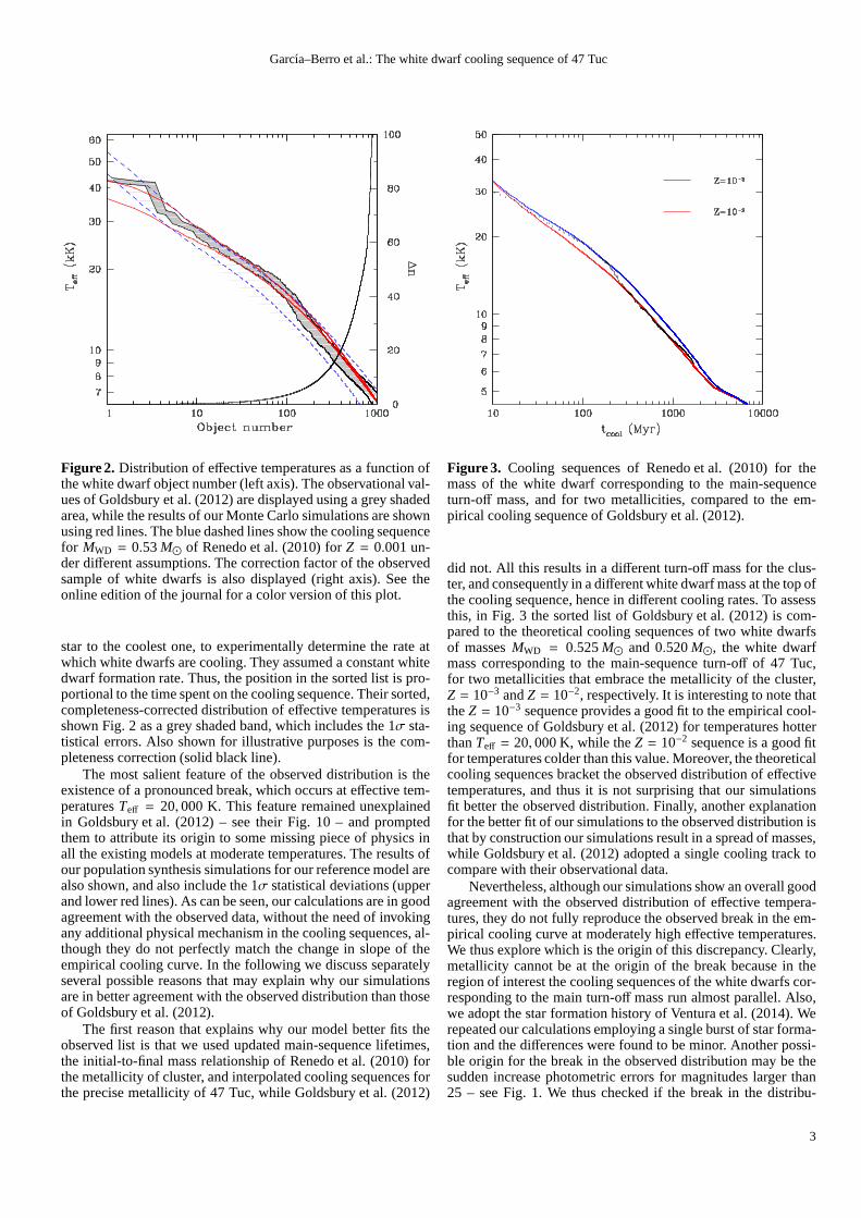
Figure 2. Distribution of effective temperatures as a function ofthe white dwarf object number (left axis). The observational val-ues of Goldsbury et al. (2012) are displayed using a grey shadedarea, while the results of our Monte Carlo simulations are shownusing red lines. The blue dashed lines show the cooling sequencefor MWD = 0.53M⊙ of Renedo et al. (2010) forZ = 0.001 un-der different assumptions. The correction factor of the observedsample of white dwarfs is also displayed (right axis). See theonline edition of the journal for a color version of this plot.

star to the coolest one, to experimentally determine the rate atwhich white dwarfs are cooling. They assumed a constant whitedwarf formation rate. Thus, the position in the sorted list is pro-portional to the time spent on the cooling sequence. Their sorted,completeness-corrected distribution of effective temperatures isshown Fig. 2 as a grey shaded band, which includes the 1σ sta-tistical errors. Also shown for illustrative purposes is the com-pleteness correction (solid black line).

The most salient feature of the observed distribution is theexistence of a pronounced break, which occurs at effective tem-peraturesTeff = 20, 000 K. This feature remained unexplainedin Goldsbury et al. (2012) – see their Fig. 10 – and promptedthem to attribute its origin to some missing piece of physicsinall the existing models at moderate temperatures. The results ofour population synthesis simulations for our reference model arealso shown, and also include the 1σ statistical deviations (upperand lower red lines). As can be seen, our calculations are in goodagreement with the observed data, without the need of invokingany additional physical mechanism in the cooling sequences, al-though they do not perfectly match the change in slope of theempirical cooling curve. In the following we discuss separatelyseveral possible reasons that may explain why our simulationsare in better agreement with the observed distribution thanthoseof Goldsbury et al. (2012).

The first reason that explains why our model better fits theobserved list is that we used updated main-sequence lifetimes,the initial-to-final mass relationship of Renedo et al. (2010) forthe metallicity of cluster, and interpolated cooling sequences forthe precise metallicity of 47 Tuc, while Goldsbury et al. (2012)

Figure 3. Cooling sequences of Renedo et al. (2010) for themass of the white dwarf corresponding to the main-sequenceturn-off mass, and for two metallicities, compared to the em-pirical cooling sequence of Goldsbury et al. (2012).

did not. All this results in a different turn-off mass for the clus-ter, and consequently in a different white dwarf mass at the top ofthe cooling sequence, hence in different cooling rates. To assessthis, in Fig. 3 the sorted list of Goldsbury et al. (2012) is com-pared to the theoretical cooling sequences of two white dwarfsof massesMWD = 0.525M⊙ and 0.520M⊙, the white dwarfmass corresponding to the main-sequence turn-off of 47 Tuc,for two metallicities that embrace the metallicity of the cluster,Z = 10−3 andZ = 10−2, respectively. It is interesting to note thattheZ = 10−3 sequence provides a good fit to the empirical cool-ing sequence of Goldsbury et al. (2012) for temperatures hotterthanTeff = 20, 000 K, while theZ = 10−2 sequence is a good fitfor temperatures colder than this value. Moreover, the theoreticalcooling sequences bracket the observed distribution of effectivetemperatures, and thus it is not surprising that our simulationsfit better the observed distribution. Finally, another explanationfor the better fit of our simulations to the observed distribution isthat by construction our simulations result in a spread of masses,while Goldsbury et al. (2012) adopted a single cooling tracktocompare with their observational data.

Nevertheless, although our simulations show an overall goodagreement with the observed distribution of effective tempera-tures, they do not fully reproduce the observed break in the em-pirical cooling curve at moderately high effective temperatures.We thus explore which is the origin of this discrepancy. Clearly,metallicity cannot be at the origin of the break because in theregion of interest the cooling sequences of the white dwarfscor-responding to the main turn-off mass run almost parallel. Also,we adopt the star formation history of Ventura et al. (2014).Werepeated our calculations employing a single burst of star forma-tion and the differences were found to be minor. Another possi-ble origin for the break in the observed distribution may be thesudden increase photometric errors for magnitudes larger than25 – see Fig. 1. We thus checked if the break in the distribu-

3

Garcıa–Berro et al.: The white dwarf cooling sequence of 47Tuc

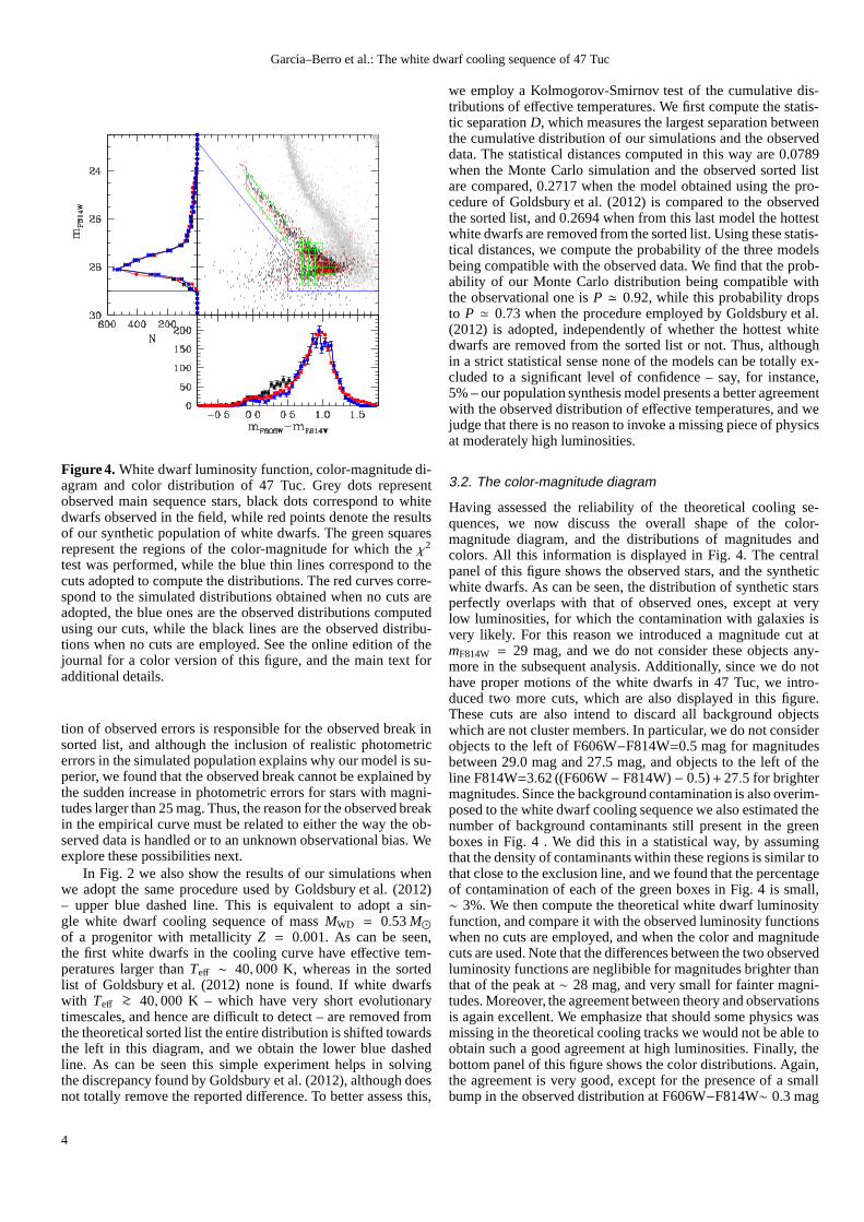
Figure 4. White dwarf luminosity function, color-magnitude di-agram and color distribution of 47 Tuc. Grey dots representobserved main sequence stars, black dots correspond to whitedwarfs observed in the field, while red points denote the resultsof our synthetic population of white dwarfs. The green squaresrepresent the regions of the color-magnitude for which theχ2

test was performed, while the blue thin lines correspond to thecuts adopted to compute the distributions. The red curves corre-spond to the simulated distributions obtained when no cuts areadopted, the blue ones are the observed distributions computedusing our cuts, while the black lines are the observed distribu-tions when no cuts are employed. See the online edition of thejournal for a color version of this figure, and the main text foradditional details.

tion of observed errors is responsible for the observed break insorted list, and although the inclusion of realistic photometricerrors in the simulated population explains why our model issu-perior, we found that the observed break cannot be explainedbythe sudden increase in photometric errors for stars with magni-tudes larger than 25 mag. Thus, the reason for the observed breakin the empirical curve must be related to either the way the ob-served data is handled or to an unknown observational bias. Weexplore these possibilities next.

In Fig. 2 we also show the results of our simulations whenwe adopt the same procedure used by Goldsbury et al. (2012)– upper blue dashed line. This is equivalent to adopt a sin-gle white dwarf cooling sequence of massMWD = 0.53M⊙of a progenitor with metallicityZ = 0.001. As can be seen,the first white dwarfs in the cooling curve have effective tem-peratures larger thanTeff ∼ 40, 000 K, whereas in the sortedlist of Goldsbury et al. (2012) none is found. If white dwarfswith Teff >∼ 40, 000 K – which have very short evolutionarytimescales, and hence are difficult to detect – are removed fromthe theoretical sorted list the entire distribution is shifted towardsthe left in this diagram, and we obtain the lower blue dashedline. As can be seen this simple experiment helps in solvingthe discrepancy found by Goldsbury et al. (2012), although doesnot totally remove the reported difference. To better assess this,

we employ a Kolmogorov-Smirnov test of the cumulative dis-tributions of effective temperatures. We first compute the statis-tic separationD, which measures the largest separation betweenthe cumulative distribution of our simulations and the observeddata. The statistical distances computed in this way are 0.0789when the Monte Carlo simulation and the observed sorted listare compared, 0.2717 when the model obtained using the pro-cedure of Goldsbury et al. (2012) is compared to the observedthe sorted list, and 0.2694 when from this last model the hottestwhite dwarfs are removed from the sorted list. Using these statis-tical distances, we compute the probability of the three modelsbeing compatible with the observed data. We find that the prob-ability of our Monte Carlo distribution being compatible withthe observational one isP ≃ 0.92, while this probability dropsto P ≃ 0.73 when the procedure employed by Goldsbury et al.(2012) is adopted, independently of whether the hottest whitedwarfs are removed from the sorted list or not. Thus, althoughin a strict statistical sense none of the models can be totally ex-cluded to a significant level of confidence – say, for instance,5% – our population synthesis model presents a better agreementwith the observed distribution of effective temperatures, and wejudge that there is no reason to invoke a missing piece of physicsat moderately high luminosities.

3.2. The color-magnitude diagram

Having assessed the reliability of the theoretical coolingse-quences, we now discuss the overall shape of the color-magnitude diagram, and the distributions of magnitudes andcolors. All this information is displayed in Fig. 4. The centralpanel of this figure shows the observed stars, and the syntheticwhite dwarfs. As can be seen, the distribution of synthetic starsperfectly overlaps with that of observed ones, except at verylow luminosities, for which the contamination with galaxies isvery likely. For this reason we introduced a magnitude cut atmF814W = 29 mag, and we do not consider these objects any-more in the subsequent analysis. Additionally, since we do nothave proper motions of the white dwarfs in 47 Tuc, we intro-duced two more cuts, which are also displayed in this figure.These cuts are also intend to discard all background objectswhich are not cluster members. In particular, we do not considerobjects to the left of F606W−F814W=0.5 mag for magnitudesbetween 29.0 mag and 27.5 mag, and objects to the left of theline F814W=3.62((F606W− F814W) − 0.5)+ 27.5 for brightermagnitudes. Since the background contamination is also overim-posed to the white dwarf cooling sequence we also estimated thenumber of background contaminants still present in the greenboxes in Fig. 4 . We did this in a statistical way, by assumingthat the density of contaminants within these regions is similar tothat close to the exclusion line, and we found that the percentageof contamination of each of the green boxes in Fig. 4 is small,∼ 3%. We then compute the theoretical white dwarf luminosityfunction, and compare it with the observed luminosity functionswhen no cuts are employed, and when the color and magnitudecuts are used. Note that the differences between the two observedluminosity functions are neglibible for magnitudes brighter thanthat of the peak at∼ 28 mag, and very small for fainter magni-tudes. Moreover, the agreement between theory and observationsis again excellent. We emphasize that should some physics wasmissing in the theoretical cooling tracks we would not be able toobtain such a good agreement at high luminosities. Finally,thebottom panel of this figure shows the color distributions. Again,the agreement is very good, except for the presence of a smallbump in the observed distribution at F606W−F814W∼ 0.3 mag

4

Garcıa–Berro et al.: The white dwarf cooling sequence of 47Tuc

when no cuts are used. However, when we discard the sourcesthat very likely are not cluster white dwarfs the agreement is ex-cellent.

As mentioned, the white dwarf cooling sequence of 47 Tuccarries interesting information about its star formation historyand age. To derive this information we use the following ap-proach. We compute independentχ2 tests for the magnitude(χ2

F814W) and color (χ2F606W−F814W) distributions. Additionally, we

calculate the number of white dwarfs inside each of the greenboxes in the color-magnitude diagram of Fig. 4 – which are thesame regions of this diagram used by Hansen et al. (2013) tocompare observations and simulations – and we perform an ad-ditionalχ2 test,χ2

N . We then investigate which are the values ofthe several parameters which define the star formation history ofthe cluster – that is, its age, the duration of the two bursts,andtheir separation – that best fit the observed data, independently.That is, we seek for the parameters of the star formation historyof 47 Tuc that best fit either the white dwarf luminosity func-tion, or the color distribution or the number of stars in eachofthe boxes in Fig. 4. Obviously, this procedure results in differentvalues of the parameters that define the star formation history of47 Tuc.

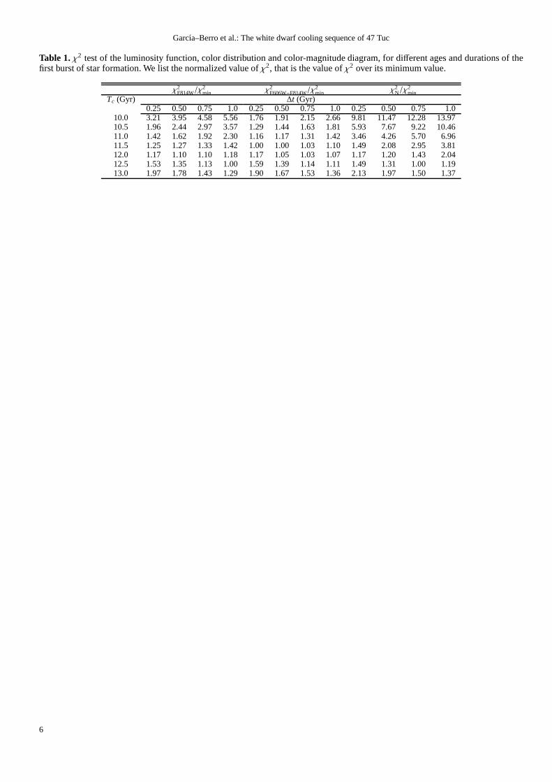
The results of our analysis are shown in Table 1, where onlythe data for a reduced set of models in which we kept fixedthe separation between the two bursts of star formation and theduration of the second burst, and varied the age of the clusterand the duration of the first burst, is listed. We remark, nonethe-less, that we explored a significantly larger range of parameters,and that for the sake of conciseness we only show here a fewmodels. We do this because we find that the values ofχ2 areless sensitive to variations in the rest of parameters, and thusthis set of models turns out to be quite representative. As canbe seen, when the white dwarf luminosity function is employedto obtain the age of the cluster and the duration of the burst ofstar formation theχ2 test favors an ageTc ≃ 12.5 ± 1.0 Gyrand a duration∆t ≃ 1.0 ± 0.5 Gyr. Instead, when the colordistribution is employed we obtainTc ≃ 11.5 ± 1.0 Gyr and∆t ≃ 0.6 ± 0.5 Gyr, respectively, while the model that best fitsthe number of stars in each bin of the color-magnitude diagramhas an ageTc ≃ 12.5 ± 0.5 Gyr and a duration of the burst ofstar formation∆t ≃ 0.7 ± 0.5 Gyr. These results are in accor-dance with those of Ventura et al. (2014), agree with the abso-lute age determination of 47 Tuc using the eclipsing binary V69(Thompson et al. 2010), and also agreee each other within theerror bars.

4. Conclusions

In this paper we have assessed the reliability and accuracy ofthe available cooling tracks using the white dwarf sequenceof47 Tuc. We have demonstrated that when the correct set of evo-lutionary sequences of the appropriate metallicity are employed,and a correct treatment of the photometric errors, and obser-vational biases is done, the agreement between the observedand simulated distributions of effective temperatures, magni-tudes and colors, as well as the general appearance of the color-magnitude diagram is excellent, without the need of invokingany missing piece of physics at moderately high effective tem-peratures in the cooling sequences. While our models do not to-tally reproduce the sudden change of slope in the empirical cool-ing sequence, it is worth noting that such change of slope takesplace in the region where the completeness correction factor be-comes relevant. Thus it might be well possible that this featuremay be only due to some unknown observational bias.

In a second phase, and given that we found that there is noreason to suspect the theoretical cooling sequences are incom-plete, we also used these distributions to study the age and starformation history of the cluster using three different distribu-tions: the white dwarf luminosity function, the color distribution,and the number counts of stars in the color-magnitude diagram.Using these three methods we obtained that the age of the clus-ter isTc ∼ 12.0 Gyr. Our results are compatible with the recentresults of Ventura et al. (2014), who found that star formation inthis cluster proceeded through two bursts, the first one of dura-tion∼ 0.4 Gyr, while the second one lasted for∼ 0.06 Gyr, sep-arated by a gap of duration∼ 0.04 Gyr. We also found that therelative strengths of these bursts of star formation activity (25%and 75%, respectively), and the presence of a helium-enhancedpopulation of white dwarf progenitors (born exclusively duringthe second burst) are also compatible with the characteristics ofthe white dwarf population.

Since our analysis of the cooling sequence of 47 Tuc closelyagrees with what is obtained studying the distribution of main-sequence stars, we conclude that a combined strategy providesa powerful tool that can be used to study other star clusters,and from this obtain important information about our Galaxy.In these sense, it is important to realize that Hansen et al. (2013)computed the age of NGC 6397, obtaining∼ 12 Gyr, signifi-cantly longer than their computed age for 47 Tuc (∼ 10 Gyr).This prompted them to suggest that there is quantitative evi-dence that metal-rich clusters like 47 Tuc formed later thanthemetal-poor halo clusters like NGC 6397. Our study indicatesthat47 Tuc is older than previously thought, and consequently, al-though this may be true, more elaborated studies are needed.

Acknowledgements. This work was partially supported by MCINN grantAYA2011–23102 by the European Union FEDER funds, by AGENCIAthroughthe Programa de Modernizacion Tecnologica BID 1728/OC-AR, and by PIP112-200801-00940 grant from CONICET. We thank R. Goldsburyand B.M.S.Hansen for providing us with the observational data shown inFigs. 2 and 4.

ReferencesAlthaus, L. G., Corsico, A. H., Isern, J., & Garcıa-Berro,E. 2010, A&A Rev.,

18, 471Bedin, L. R., King, I. R., Anderson, J., et al. 2008a, ApJ, 678, 1279Bedin, L. R., Salaris, M., King, I. R., et al. 2010, ApJ, 708, L32Bedin, L. R., Salaris, M., Piotto, G., et al. 2008b, ApJ, 679,L29Bedin, L. R., Salaris, M., Piotto, G., et al. 2005, ApJ, 624, L45Bellini, A., Bedin, L. R., Piotto, G., et al. 2010, A&A, 513, A50Garcıa-Berro, E., Torres, S., Althaus, L. G., et al. 2010, Nature, 465, 194Garcıa-Berro, E., Torres, S., Isern, J., & Burkert, A. 1999, Month. Not. Roy.

Astron. Soc., 302, 173Garcıa-Berro, E., Torres, S., Isern, J., & Burkert, A. 2004, Astron. & Astrophys.,

418, 53Goldsbury, R., Heyl, J., Richer, H. B., et al. 2012, ApJ, 760,78Hansen, B. M. S., Brewer, J., Fahlman, G. G., et al. 2002, ApJ,574, L155Hansen, B. M. S., Kalirai, J. S., Anderson, J., et al. 2013, Nature, 500, 51Kalirai, J. S., Richer, H. B., Anderson, J., et al. 2012, AJ, 143, 11Kroupa, P., Tout, C. A., & Gilmore, G. 1993, MNRAS, 262, 545Milone, A. P., Piotto, G., Bedin, L. R., et al. 2012, ApJ, 744,58Renedo, I., Althaus, L. G., Miller Bertolami, M. M., et al. 2010, Astrophys. J.,

717, 183Salaris, M., Althaus, L. G., & Garcıa-Berro, E. 2013, A&A, 555, A96Thompson, I. B., Kaluzny, J., Rucinski, S. M., et al. 2010, AJ, 139, 329Torres, S., Garcıa-Berro, E., Burkert, A., & Isern, J. 2002, MNRAS, 336, 971Ventura, P., Criscienzo, M. D., D’Antona, F., et al. 2014, MNRAS, 437, 3274Woodley, K. A., Goldsbury, R., Kalirai, J. S., et al. 2012, AJ, 143, 50

5

Garcıa–Berro et al.: The white dwarf cooling sequence of 47Tuc

Table 1. χ2 test of the luminosity function, color distribution and color-magnitude diagram, for different ages and durations of thefirst burst of star formation. We list the normalized value ofχ2, that is the value ofχ2 over its minimum value.

χ2F814W/χ

2min χ2

F606W−F814W/χ2min χ2

N/χ2min

Tc (Gyr) ∆t (Gyr)0.25 0.50 0.75 1.0 0.25 0.50 0.75 1.0 0.25 0.50 0.75 1.0

10.0 3.21 3.95 4.58 5.56 1.76 1.91 2.15 2.66 9.81 11.47 12.28 13.9710.5 1.96 2.44 2.97 3.57 1.29 1.44 1.63 1.81 5.93 7.67 9.22 10.4611.0 1.42 1.62 1.92 2.30 1.16 1.17 1.31 1.42 3.46 4.26 5.70 6.9611.5 1.25 1.27 1.33 1.42 1.00 1.00 1.03 1.10 1.49 2.08 2.95 3.8112.0 1.17 1.10 1.10 1.18 1.17 1.05 1.03 1.07 1.17 1.20 1.43 2.0412.5 1.53 1.35 1.13 1.00 1.59 1.39 1.14 1.11 1.49 1.31 1.00 1.1913.0 1.97 1.78 1.43 1.29 1.90 1.67 1.53 1.36 2.13 1.97 1.50 1.37

6