The Welfare Effects of Peer Entry in theAccommodation Market: The Case of Airbnb1

Chiara Farronato2 and Andrey Fradkin 3

October 18, 2017

PRELIMINARY AND INCOMPLETE

PLEASE DO NOT DISTRIBUTE OR CITE WITHOUT PERMISSION

Abstract

We study the entry of Airbnb into the accommodation industry and its effects

on travelers, hosts, and hotels. We first document heterogeneity in Airbnb’s

penetration across 50 major US cities and demonstrate that much of this het-

erogeneity can be explained by proxies for hotel costs, the costs of peer hosts,

and demand fluctuations. Next, we document that Airbnb has an effect on hotel

revenues. This effect is mostly due to a reduction in hotel prices rather than

occupancy and is greatest in cities with low hotel capacity relative to the size of

demand. Finally, we estimate a structural model of competition between peer

hosts and hotels and use it to study the effects of Airbnb on the distribution of

surplus across consumers, peer hosts, and incumbent hotels. We find an average

consumer surplus of $70 per night from Airbnb. This surplus is disproportion-

ately concentrated in locations (New York) and times (New Year’s Eve) when

hotels have high occupancy. Because Airbnb guests view Airbnb as a differenti-

ated product and because Airbnb bookings occur disproportionately when hotels

are near full capacity, most of these bookings would not have resulted in hotel

bookings had Airbnb not been available. We also quantify the effects on hotels

1Katie Marlowe and Max Yixuan provided outstanding research assistance. We thank Nikhil Agarwal,Susan Athey, Matt Backus, Liran Einav, Christopher Knittel, Jonathan Levin, Greg Lewis, Chris Nosko,Debi Mohapatra, Ariel Pakes, Paulo Somaini, Sonny Tambe, Dan Waldinger, Ken Wilbur, Giorgos Zervas,and numerous seminar participants for feedback. We are indebted to Airbnb’s employees, in particular PeterColes, Mike Egesdal, Riley Newman, and Igor Popov, for sharing data and insights. Fradkin is a formeremployee of Airbnb.

2Harvard Business School and NBER, cfarronato@hbs.edu3MIT Sloan School of Management, afradkin@mit.edu

and peer hosts. In total, the sum of the surplus from Airbnb entry across con-

sumers, hotels, and hosts is $352 million in 2014 for the top 10 US cities in terms

of Airbnb’s penetration.

2

1 Introduction

The Internet and related technologies have greatly reduced entry and advertising costs across

a variety of industries. As an example, peer-to-peer marketplaces such as Airbnb, Uber, and

Etsy to provide a platform for small and part-time service providers (peers) to participate

in economic exchange. Several of these marketplaces have grown quickly and have become

widely known brands. In this paper, we study the determinants and effects of peer production

in the market for short-term accommodation, where Airbnb is the main peer-to-peer platform

and hotels are incumbent suppliers. Specifically, we present a theoretical model of peer

competition with traditional firms and use the example of Airbnb to estimate the model and

quantify the effects of Airbnb on consumers, hotels, and Airbnb hosts.

Since its founding in 2008, Airbnb has grown to list more rooms than any hotel group

in the world. Yet Airbnb’s growth across cities and over time has been heterogeneous, with

supply shares ranging from over 15% to less than 1% across major US cities at the end of

2014. We propose a theoretical framework based on economic fundamentals to explain this

heterogeneity. In our framework, accommodations can be provided by either dedicated or

flexible supply – hotels vs peer hosts. The main difference between dedicated and flexible

producers is that dedicated producers have higher investment costs while flexible sellers

typically have higher marginal costs.

The role of Airbnb in our framework is to lower entry costs for flexible producers. This

reduction in entry costs is similar across geographies but the benefits of renting accommo-

dations vary. In the long-run, the entry of flexible producers is driven by the trend and

variability of demand in a given city, hotel investment costs, and peer rental costs. We

confirm that these predictions hold in our data.

In the short-run, flexible producers decide whether to host on a particular day. Because

of the flexible nature of their supply, we hypothesize that these producers will be highly

responsive to market conditions, hosting travelers when prices are high, and using accom-

modation for private use when prices are low. In contrast, because hotels have only rooms

dedicated to travelers’ accommodation, they will typically choose to transact even when

demand is relatively low. We validate this prediction by documenting that the elasticity of

supply is 92% higher for flexible producers than for hotels.

Next, we estimate a model of short-run equilibrium and use it to quantify the effect of

Airbnb on total welfare and its distribution across travelers, peer hosts, and hotels. Travelers

benefit from Airbnb for two reasons. First, flexible sellers offer a differentiated product

relative to hotels. Second, they also compete with hotels by expanding the number of rooms

available. This second effect is particularly important in periods of high demand when

3

hotels are capacity constrained and have high market power. Consequently, we find that the

consumer surplus is concentrated in cities where hotel expansion is restricted and in periods

of high demand. In those cities and periods, flexible sellers allow more travelers to stay in a

city without greatly affecting the number of travelers staying at hotels.

We enumerate our main quantitative results below, where the sample consists of the ten

largest cities in terms of Airbnb share in the US for 2014. First, consumer surplus per night

booked on Airbnb is $70, and 71% of this surplus comes from the fact that Airbnb listings

are preferred to hotels by a share of consumers at prevailing prices. The rest of the surplus

is due to Airbnb’s negative effect on hotel prices. This effect is largest when hotels have

market power due to being at or near full capacity. The total consumer surplus gain from

Airbnb is $432 million, with the largest gains coming in New York City. Second, we find

that over 70% of Airbnb bookings would not have been hotel stays had Airbnb not existed.

Third, the entry of Airbnb results in a 1% loss in hotel revenues in this sample. Lastly, peers

receive an average of $28 in surplus per night, resulting in a host surplus of $20 million in

2014.

Our data mainly comes from two sources: proprietary Airbnb data and Smith Travel

Research (STR), a hotel industry data aggregator. For both datasets, we prices and occu-

pancy rates at a city, day, and accommodation type level between 2011 and 2014 for the

50 largest US cities.1 We use this data to document heterogeneity in the number of Airbnb

listings across cities and over time. Cities like New York and Los Angeles have grown quickly

in terms of available rooms on Airbnb, while cities like Oklahoma City and Memphis have

grown at lower rates. Within each city over time, the number of available rooms is higher

during peak travel times such as Christmas and the summer. The geographic and time het-

erogeneity suggests that hosts flexibly choose when to list their rooms for rent on Airbnb,

and are more likely to do so in cities and times when the returns to hosting are highest.

In section 2, we incorporate this intuition into a model of the market for accommoda-

tions. In this model, hosting services can be provided by dedicated or flexible sellers, and

products are differentiated. Dedicated sellers are characterized by high investments costs,

but low marginal costs. Since dedicated capacity is always available to travelers and has

no alternative use, investment in dedicated capacity is justified when rooms are frequently

occupied. Instead, flexible capacity does not require any investment but typically involves

higher marginal costs to operate. On Airbnb, hosts do not always have a room available for

rent, and when they do, they must prepare the room and interact with the guests before and

during the trip. Hosting is also perceived as risky by some individuals.

Our model includes two time-horizons. The long-run horizon is characterized by the entry

1The 50 largest US cities were selected on the basis of their total number of hotel rooms.

4

decision of flexible sellers given the new Airbnb platform. The short-run horizon focuses on

daily prices and quantities of rooms rented, taking flexible and dedicated capacity as given.

We model the decision of flexible sellers to join the platform as dependent on the expected

returns from hosting, which depends in turn on competition from hotels and overall demand.

We define the short-run horizon as one day in one city. In the short-run, the capacity of

flexible and dedicated sellers is fixed. Travelers choose an accommodation option among

differentiated products, e.g. luxury vs economy hotels, and hotels vs Airbnb rooms. The

demand for these goods varies over time due to market-wide demand fluctuations, such as

seasonality, and idiosyncratic product-specific demand shocks (e.g. Berry et al. (1995)). On

the supply side, hotels compete in a Cournot game with differentiated products subject to

capacity constraints and with a competitive fringe of Airbnb hosts. Hosts take prices as

given and host travelers if the market clearing price on the platform is greater than their

cost of hosting.

The model offers testable predictions. The long-run share of flexible sellers should differ

across cities. Entry should be largest in cities where hotel investment costs are high, flexible

sellers’ marginal costs are low, and demand variability is high so that there are periods of high

prices. In the short-run, flexible sellers should increase competition: they will reduce prices

and occupancy rates of hotels, and the effects will be largest in cities where hotel capacity

is low relative to demand. We describe those cities as having constrained hotel capacity. In

those cities, the model predicts that Airbnb reduces prices more than occupancy rates.

In section 3, we confirm that these model predictions hold in the data. We first look

at the long-run patterns. We show that peer supply as a share of total supply is larger in

cities where hotel prices are higher. These high prices are associated with the difficulty of

building hotels due to regulatory or geographic constraints. Peer supply is also larger in

cities where residents tend to be single and have no children. These residents likely have

lower costs of hosting strangers in their homes. Another factor influencing peer supply is

the volatility of demand. A city can experience periods of high and low demand due to

seasonality, festivals, or sporting events. When the difference in peaks and troughs is large,

the provision of accommodation exclusively by hotels can be inefficiently low. We show that

Airbnb’s supply share is larger precisely in cities with high demand volatility, and, perhaps

more intuitively, in cities where demand growth is high.

We then test the predictions of the model on short-run hotel outcomes. We do this by

estimating regressions of hotel outcomes on a measure of Airbnb supply using two types of

instruments as well as controls for aggregate demand shocks. Measurement and endogeneity

challenges are discussed in subsection 3.2. On average, a 10% increase in the number of

available listings on Airbnb reduces hotel revenues by 0.36%. This effect is mostly due to

5

a reduction in hotel prices rather than a decrease in occupancy rates and is heterogeneous

across cities. The effect is larger in cities with constrained hotel capacity, where a 10%

increase in Airbnb listings decreases hotel prices by 0.52%. In other cities, the reduction is

quantitatively small and statistically insignificant. The heterogeneity in estimates is due to

differences in both the size of Airbnb and the effects of Airbnb across markets conditional

on that size. The magnitude of the reduced form coefficient and the finding of greater effects

on pricing is broadly in line with the work of Zervas et al. (2015), who focus on the average

effects of Airbnb on hotels in Texas.

In section 4, we describe our estimation strategy for recovering the primitives of the

model from section 2. Our estimation strategy combines a random coefficient multinomial

logit demand model (Berry et al. (1995)) with hotels’ pricing decisions. In order to take

into account the fact that prices steeply increase when occupancy reaches hotel capacity, we

follow Ryan (2012) and rationalize these price changes with increasing marginal costs that

operate when hotels are close to their capacity constraint. We also augment our estimation

with survey data regarding the preferred second choices of Airbnb travelers. Finally, we

estimate the marginal cost distribution of hosts on Airbnb assuming that they are price

takers. Together, these estimates allow us to measure consumer and peer producer surplus,

as well as to quantify how surplus would change in the absence of the Airbnb platform.

Section 5 presents our results. We find that consumers’ utility for Airbnb is lower than

for hotels, but that preferences for Airbnb increase between 2013 and 2014. By the end of

the sample period, the mean utility from top quality Airbnb listings is close to the mean

utility of economy and midscale hotels in cities with a large Airbnb presence. Consistent

with our model, we find that flexible sellers have higher marginal costs than dedicated sellers

on average, and that the distribution of peer costs makes flexible supply highly elastic.

In the absence of Airbnb, total welfare would be lower and travelers and peer producers

would be worse off. However, hotels would gain from the reduced competition. We find

that for New York, the city with the largest Airbnb supply in our sample, consumer surplus

would be $207 million lower if Airbnb did not exist in 2014. This corresponds to a consumer

surplus of $69 per night for every Airbnb booking in New York.

The reduction in consumer surplus if Airbnb did not exist occurs because fewer travelers

would book rooms, and travelers who end up booking hotel rooms would pay higher prices.

As it turns out, because of the elastic supply of Airbnb rooms, actual Airbnb bookings, and

hence surplus gains, disproportionately occur in cities (New York) and times (New Year’s

Eve) when hotel capacity constraints bind. This implies that in the absence of Airbnb,

travelers could not easily find a substitute hotel room because hotels would be fully booked.

Indeed, we find that over half of Airbnb bookings would not have been hotel stays had

6

Airbnb not existed.

The concentration of Airbnb bookings in cities and periods of peak demand suggests that

in the absence of Airbnb, hotels would be limited in their ability to increase the number of

booked rooms – they are already operating at or close to full capacity – but instead would be

able to increase prices. This is consistent with our reduced form evidence, and it is precisely

what we see in our counterfactuals. Revenues for hotels in New York would increase by 1.5%

if Airbnb did not exist and a measure of profits would increase by 3.05%.

The growth of peer production in the accommodations industry is important to study

because of its business and regulatory implications. As Airbnb grows, other actors in the

industry such as hotels, OTAs, and peer hosts must learn how to adopt. Second, many cities

wish to regulate the peer producers in the accommodation industry but there has been much

disagreement regarding the specific form of this regulation. If Airbnb only affected hotels,

travelers, and peer hosts, then our results suggest that the net contribution of Airbnb is

positive. However, there are potential effects on housing, labor markets, and the neighbors

of hosts that we do not consider in this paper and leave for future research.

We contribute to the growing empirical literature on online peer-to-peer platforms. A

limited number of papers have looked at the effect of online platforms on incumbents, in

particular Zervas et al. (2015) for Airbnb, Seamans and Zhu (2014) and Kroft and Pope

(2014) for Craigslist, and Aguiar and Waldfogel (2015) for Spotify. We estimate the effects

not only on incumbent firms but also on consumers and new producers. Furthermore, we

are able to document how these effects vary over time and across cities and conduct coun-

terfactual simulations. Another complementary paper to ours is Cohen et al. (2016), which

uses discontinuities in Uber’s surge pricing policy to estimate the consumer surplus from ride

sharing. Both of our papers find that successful peer-to-peer platforms generate substan-

tial consumer surplus. However, the mechanisms which generate this surplus differ between

our papers. While Cohen et al. (2016) assume that market structure remains constant, we

incorporate capacity constraints and allow for hotel prices to adjust endogenously. This is

important for our setting because even hotel customers benefit from Airbnb since they pay

lower prices. Relatedly, Lam and Liu (2017) estimate a model of competition between Uber,

Lyft, and taxis using data from New York.

Another related stream of work studies the role of peer-to-peer markets in enabling rental

markets. The premise of these papers is that technology has made it easier to borrow and

rent assets. Horton and Zeckhauser (2016) derive a theoretical model of equilibrium for assets

and make predictions on the existence and size of rental markets across different product

categories. Fraiberger and Sundararajan (2015) calibrate a model of car usage and make

predictions on the reduction in car ownership as a result of peer-to-peer rental markets. Our

7

work does not specifically study the decision to own or rent apartments, but it explicitly

quantifies the benefits from renting on Airbnb.

Our paper is also complementary to existing studies of labor supply and market design

on peer-to-peer platforms. We find that host supply is highly elastic on the margin. This is

consistent with analysis of suppliers on Taskrabbit (Cullen and Farronato (2014)) and Uber

(Hall et al. (2016), Chen and Sheldon (2015)). Other work on peer-to-peer markets has fo-

cused on the market design aspects of reputation systems (Fradkin et al. (2017), Nosko and

Tadelis (2015), Bolton et al. (2012)), search (Fradkin (2015), Horton (2016)), and pricing

(Einav et al. (Forthcoming), Hall et al. (2016)). Lewis and Zervas (2016) study the welfare

effects of online reviews in the hotel industry. Finally, in our analysis of growth hetero-

geneity across cities, we contribute to the predominantly theoretical literature on technology

adoption and diffusion (e.g. Bass (1969) and Griliches (1957)).

The paper is structured as follows. In the next section, we present the data and document

geographic and time heterogeneity in the size of Airbnb, which motivates our theoretical

framework for market structure with flexible and dedicated supply (Section 2.1). In Section

3 we test the basic predictions of our model on the long- and short-run elasticities of flexible

supply, and on the spillover effects of Airbnb on hotels. Section 4 presents our empirical

strategy for estimating the short-run equilibrium of our model. We discuss the estimation

results in Section 5 and conclude in Section 6.

2 Motivation and Theoretical Framework

Airbnb describes itself as a trusted community marketplace for people to list, discover,

and book unique accommodations around the world — online or from a mobile phone. The

marketplace was founded in 2008 and has at least doubled in total transaction volume during

every subsequent year. Airbnb has created a market for a previously rare transaction: the

short-term rental of an apartment or room to strangers. In the past, these transactions

were not commonly handled by single individuals because there were large costs to finding

a match, securely exchanging money, and ensuring safety. While Airbnb is not the only

company serving this market, it is the dominant platform in most US cities.2 Therefore, we

use Airbnb data to study the drivers and the effects of facilitating peer entry in the market

for short-term accommodations.

Airbnb room supply has grown quickly in the aggregate, but the growth has been highly

2The most prominent competitor is Homeaway/VRBO, a subsidiary of Expedia. Its business has his-torically been concentrated in rentals of entire homes in vacation destinations, such as beach and skiingresorts.

8

heterogeneous across geographies. Figure 1 plots the size of Airbnb measured as the daily

share of available Airbnb listings out of all rooms available for short-term accommodation.3

Even among the top 10 cities in terms of listings, there are high growth markets like San

Francisco and New York, as well as slow growth markets like Chicago and DC. This increase

in available rooms is specific to the peer-to-peer sector and does not represent a broader

growth of the supply of short-term accommodation (see Figure A1).

Within a city over time, there is also heterogeneity in the size of Airbnb relative to the

size of the hotel sector. The fluctuations are especially prominent in New York in Figure

1, which experiences large spikes in available rooms during New Year’s Eve, and in Austin

during the South by Southwest festival. The figure suggests that market conditions during

these spikes are especially suited to peer-to-peer transactions. These facts motivate our

theoretical model, in which we distinguish between dedicated sellers (hotels) and flexible

sellers (peer hosts).

2.1 Theoretical Framework

In this section, we introduce a theoretical model for understanding market structure with

dedicated supply (hotels) and flexible supply (peer hosts) in the accommodation industry.

We will test the predictions of this model in Section 3, and structurally estimate it in Section

4.

In our model, hosting services can be provided by professional and flexible sellers, who

offer differentiated products. The model has a short and long-run component. The short-

run equilibrium consists of daily prices and rooms sold of each accommodation type as a

function of a demand state and the respective capacities of dedicated and flexible suppliers.

We assume hotels are competing against a fringe of flexible sellers. The long-run component

determines the entry condition of flexible sellers as a function of a fixed hotel capacity and

the distribution of demand states.

We start by presenting the short-run equilibrium, which we view as an analog to daily

market outcomes. We simplify the exposition by assuming that there is one single hotel

and one undifferentiated type of Airbnb listings. In the empirical counterpart of this model

presented in section 4, we relax this assumption. Let Kh denote the existing dedicated

capacity (number of hotel rooms), and Ka the existing flexible capacity (Airbnb rooms).

Demand state, d, is drawn from a distribution F , which can be interpreted as the distribution

of demand states over the course of a year. Hotel rooms and Airbnb rooms are differentiated

3The total number of available rooms is the sum of available hotel rooms and listings available on Airbnb.The same heterogeneity is apparent if we adjust for capacity, or if we divide the number of Airbnb listingsby the number of total housing units within an MSA.

9

products. Qdi (pi, pj) is the residual demand for product i as a function of its price and the

price of the other product. Qdi (pi, pj) is increasing in d and pj, and decreasing in its own

price pi.

The short-run sequence of events is as follows. Capacity Kh and Ka are given, demand

state d is realized, the hotel sets prices and at the same time Airbnb sellers choose whether

to host. We assume that the hotel faces marginal cost ch to book one room for one night,

and it sets its price to maximize profits subject to its capacity constraint:

Maxph

Qdh(ph, pa)(ph − ch)

s.t. Qdh(ph, pa) ≤ Kh

(1)

Flexible sellers have unit capacity and variable marginal costs of renting their room. We

assume that marginal costs of peers are randomly drawn from a known distribution, and

that on average are higher than ch. When choosing whether to rent our their room for a

night, flexible producers take prices as given, and sell their unit if and only if the market

clearing price is greater than their cost. The choices of individual hosts are aggregated to

determine the total number of flexible rooms rented:

Qda(pa, ph) = KaPr(c ≤ pa), (2)

where Ka is the mass of peer hosts, or total flexible capacity.

The market equilibrium consists of prices and quantities for the hotel and peers (ph, pa, qh, qa)

that equate flexible and dedicated room demand with flexible and dedicated supply.

The short-run model already offers some comparative statics predictions, listed below and

proven in Appendix A. Under standard conditions, hotel profits per available room, as well

as both prices and occupancy rates, are lower if Ka is higher (Proposition 1 in the appendix).

The separate effect of an increase in Ka on hotel prices is higher if hotel capacity constraints

are more often binding, but the opposite is true for the effect on occupancy (Proposition

2). Intuitively, this occurs because the increase in flexible capacity affects hotels through

a reduction in their residual demand (Figure 2), and when hotels are capacity constrained,

their supply curve is vertical (Figure 2a). A marginal downward shift in residual demand

will have no effect on quantity and a large effect on price if supply is perfectly inelastic.

In the long-run, entry of flexible suppliers is endogenous. We assume that Kh was opti-

mally set knowing F (d) and not expecting that Airbnb would lower entry costs of flexible

sellers. Holding demand fixed, if investing in hotel capacity is more costly, optimal dedicated

capacity is lower and expected profits per unit of capacity are higher.

A peer-to-peer platform enables the entry of flexible sellers. Flexible sellers decide

10

whether to join the peer-to-peer platform and start producing as a function of expected

demand. We assume that flexible sellers face a cost, C, of joining the platform, which is

randomly drawn from a given distribution and that their time horizon coincides with the dis-

tribution of demand states F . Let va =∫dEc(max{0, pda − c}

)dF (d). Ec

(max{0, pda − c}

)is the expected profit of a flexible seller given demand state d, and the expectation is taken

over the distribution of marginal costs.

A flexible seller joins the peer-to-peer platform if va ≥ C. If expected profits va are higher,

more flexible sellers will join the platform and start producing, and the share of flexible supply

out of total supply will be higher. What affects va? The first element is the distribution of

marginal costs c. Holding everything else constant, if the distribution of costs decreases in

the sense of first order stochastic dominance, more peers will enter and start hosting. The

second element is pda, itself a function of Kh and the distribution of demand F (d). All else

equal, a lower Kh will increase equilibrium prices whenever capacity constraints bind, so it

will increase the distribution of pda in the first order stochastic dominance sense. Clearly, a

higher level of demand in every state is more attractive, but, perhaps less obviously, also

an increase in demand variability is attractive for flexible suppliers. To explain why we

can think of a simple mean-preserving spread of two demand states. In the low demand

state, flexible suppliers host very few travelers in either case because hotels’ low marginal

costs imply low equilibrium prices. The difference occurs in high demand states. If the

high demand state doubles, prices increase steeply, especially if hotel capacity constraints

are hit, making it very attractive for flexible suppliers to host in periods of high demand.

Appendix A formally states these comparative statics results in Proposition 3 and provides

formal proofs. Section 3.2 confirms that these comparative statics predictions hold in the

data.

One final aspect of our model is that it does not allow hotels to adjust dedicated capacity

Kh in response to peer entry. In the long-run, peer entry could partially crowd out dedicated

sellers. Since our data only spans the first few years of Airbnb diffusion, we are unable to

empirically capture hotels’ capacity adjustments. Exploring the entry and exit decisions of

dedicated producers would be a valuable extension of our work.

3 Data and Tests of the Model

In this section, we describe our data on Airbnb and hotels and document how it confirms the

predictions of the theoretical framework. Our proprietary Airbnb data consists of information

aggregated at the level of listing types. The variables we observe include the number of

bookings, active and available listings, as well as average listed and transacted prices. An

11

available listing is defined as one that is either booked through Airbnb or is open to being

booked on the date in question according to a host’s calendar. An active room is defined as

a listing that is available to be booked on the calendar or is available for at least one date

in the future.

We categorize Airbnb listings into four types: ’Airbnb Luxury’, ’Airbnb Upscale’, ’Airbnb

Midscale’, and ’Airbnb Economy’.4 Listing types are defined using the following algorithm.

We first run a city level hedonic regression of nightly price on listing fixed effects, date

fixed effects, and bins for the number of five-star reviews.5 Second, we extract the listing

fixed effects and use Bayesian shrinkage to shrink fixed effects towards the mean. Third, we

compute quartiles of listing quality and categorize a listing in a given quartile if its fixed effect

plus review coefficient falls into the appropriate range. This procedure allows us to account

for heterogeneity in Airbnb listing types without specifically modeling detailed geographic

and room type characteristics at a city level.

The hotel data come from Smith Travel Research (STR), an accommodation industry

data provider that tracks over 161,000 hotels. Our sample contains daily prices and occu-

pancy rates for the 50 largest US cities for the period between January 2011 and December

2014.6 STR obtains its information by running a periodic survey of hotels. For the 50

largest markets, 68% of properties are surveyed, covering 81% of available rooms. STR uses

supplementary data on similar hotels to impute outcomes for the remaining hotels which are

in their census but do not participate in the survey. The data is then aggregated to six hotel

scales, from luxury to economy, which indicate the quality and amenities of the hotels.

Table 1 shows city-level descriptive statistics regarding hotels and Airbnb. In the average

city, hotels charge $108 per room and their occupancy rate is 66%. Perhaps surprisingly,

Airbnb has very similar transacted prices ($109) and much lower occupancy rates (15%). The

within-city standard deviation of these outcomes varies greatly across cities. For example,

the city at the 25th percentile has a standard deviation of hotel prices of $10 ($22 for Airbnb

prices), while the city at the 75th percentile has a standard deviation of $21 ($34 for Airbnb

prices). This indicates that markets differ not only in levels but in the extent to which

conditions fluctuate within a year and over time.

During our sample period, Airbnb comprises a small share of the overall market as a

percentage of total rooms available for short-term accommodation. The average Airbnb

4These categories are defined solely for the purpose of this paper and do not correspond to any metricused by Airbnb itself.

5The bins for the number of reviews are: 0, 1, 3, 5, 10, 25, 50, 100.6The cities are ranked based on the absolute number of hotel rooms in 2014. See Census Database: http:

//www.str.com/products/census-database and STR Trend Reports: http://www.str.com/products/

trend-reports

12

share of available rooms in the last quarter of 2014 is 2%, and in most cities it is between

1% and 3% (25th and 75th percentiles). Two other normalizations confirm that Airbnb

was still small in most US cities by the end of our sample period. Across all cities, Airbnb

rooms represent 4% of all guests and represent less than 1% of total housing units for all

metropolitan statistical areas (MSAs) in our sample.

3.1 The Long-Run: Determinants of Peer Entry

In this section, we verify the theoretical predictions regarding the long-run growth of peer

supply from Section 2.1. Although the theoretical model assumes that entry decisions are

made instantaneously and jointly for all flexible sellers, in practice awareness about the

Airbnb platform has slowly spread in our sample period, 2011 to 2014. We assume that the

last quarter in 2014, the end of our sample, provides a valid approximation to the long-run

share of peer supply derived in our model.

Figure 3 shows the relationship between Airbnb market share and hotel revenues per

available room. Not surprisingly, the size of Airbnb is positively correlated with the average

revenue per room in a city, with New York being both the city with the highest hotel revenues

and the one with the highest penetration of peer hosts.

In Section 2.1 we presented our theoretical framework, which links the profitability of

hosting for flexible sellers in a given city to the relative costs of hotels versus peer hosts.

If hotels’ investment costs are high or peer hosts have low marginal costs, profitability for

peer hosts will be high. This implies more peer entry in cities with high hotel investment

costs and low marginal costs of peers. We use two proxies for the first cost factor, i.e. hotel

capacity investment costs. The first is the share of undevelopable area constructed by Saiz

(2010). The index measures the share of a metropolitan area that is undevelopable due to

geographic constraints, e.g. bodies of water or steep mountains. The second index is the

Wharton Residential Land Use Regulatory Index (WRLURI), which measures the amount

of regulation required for land use in each metropolitan area and is based on a nationwide

survey described in Gyourko et al. (2008).7 Figures 4a and A2 confirm that constraints to

hotel capacity are correlated with Airbnb penetration in a city.8

The second cost factor influencing the viability of peer production is the marginal cost

of peers. Although many factors affect the costs of hosting, we focus on those related to

7Saiz (2010) uses these two measures to calculate the housing supply elasticity at the level of a metropoli-tan area.

8Building restrictions also affect Airbnb supply through another channel, the cost of residential housing.There are greater incentives to monetize a spare bedroom when the costs of housing are higher, especiallyfor liquidity constrained households. Figure A2 in the Appendix confirms a positive relationship betweenthe share of household income used to pay rent in 2010 and the size of Airbnb in 2014.

13

demographics.9 Households vary in their propensities to host strangers in their homes. For

example, an unmarried 30-year-old professional will likely be more open to hosting strangers

than a family with children. This occurs for at least two reasons. First, children increase a

host’s perceived risk of the transaction. Second, unmarried professionals are more likely to

travel, creating vacant space to be rented on Airbnb. Figure 4b plots the share of flexible

supply at the end of 2014 against the percentage of unmarried adults, while Appendix Figure

A2 uses the percentage of children. The figures confirm that cities with more unmarried

adults and fewer children are those where Airbnb has indeed spread more.

In addition to cost factors, our model predicts that travelers’ demand affects peer entry.

This is due to two related reasons. First, hotels typically do not have enough dedicated

capacity to absorb all potential travelers in times of peak demand. In contrast, flexible sellers

are able to provide additional supply during peak times, when their rooms are especially

valuable to travelers. Second, since hotels must pre-commit to capacity and any adjustment

in the form of new hotel buildings takes 3 to 5 years, unforeseen growth in demand will

create an inefficiently low dedicated supply and will induce entry by flexible sellers.

We use data from air travelers to proxy for accommodation demand trends and fluc-

tuations at the city-month level. Our data come from Sabre Travel Solutions, the largest

Global Distribution Systems provider for air bookings in the US. We isolate trips entering a

city as part of a round trip from a different city in order to measure the potential demand

for short-term stays.10 Figure 5a confirms the intuition that unexpected growth in demand

will result in greater peer entry by showing that the 2012-2011 growth rate in travelers for

each city is positively related to Airbnb penetration in 2014. Figure 5b plots the standard

deviation of demand in 2011 and confirms that by the end of 2014 Airbnb is bigger in cities

where the fluctuations in the number of arriving travelers are larger.

To conclude this section, we combine all the descriptive results into a regression. Table

2 displays the summary statistics for the cost and demand factors described above. Table

3 displays results from a regression where the dependent variable is the size of Airbnb in

the last quarter of 2014 and the explanatory variables are combinations of the measures of

relative costs, demand growth, and demand variability described above. We also control for

market size in order to isolate the component of the standard deviation of demand which

is due to demand variability. Despite the small sample size, column (1) shows that all

factors affect the size of Airbnb in the expected direction, and two - peers’ marginal costs,

and demand volatility - are statistically significant. Column (2) adds an additional, and

9Other potential shifters of the returns to hosting include household liquidity constraints, building regu-lation and enforcement of short-term rentals, and the ease of vacating an apartment in high demand periods

10Observations in the underlying Sabre provides data on the number of passengers, the origin airport, andthe destination airport for a given month. We aggregate these to an MSA-month measure of passengers.

14

potentially redundant measures of our proxies. The coefficients are in the expected direction

for all proxies.

The last column of Table 3 suggests that demand proxies and hotel investment costs

affect peer entry mostly through price. In column (3) we add the average revenue per room

in 2011 as an additional control. We choose the 2011 average because it is not affected

by subsequent peer entry. The coefficient on revenue per available room is positive and

statistically significant. In addition, the coefficients on the demand and hotel investment

cost proxies decrease in magnitude and become insignificant, which supports our theoretical

model. Taken altogether, our proxies for the determinants of long-run peer supply explain

almost 75% of the variation across the sample of 46 cities.

3.2 The Short-Run: Effects of Peer Entry on Hotels

In the previous section we have tested the long-run predictions of our theoretical model,

those related to the entry of peer producers. Here, we take entry as given, and focus on the

short-run drivers of peer supply, and the effects of peer supply on hotels. The awareness and

diffusion process of Airbnb and its variation across cities help us identify the causal impact

of Airbnb on hotel revenues.

First, we show how to properly measure the size of Airbnb, and how the short-run

elasticity of Airbnb supply is twice as large as that of hotels. Then, we use an instrumental

variable approach to study the reduction in hotel revenues caused by the entry of Airbnb,

and its heterogeneity across cities and hotel scales.

Measuring Airbnb Supply

We start by demonstrating how to properly measure Airbnb supply and studying how hosts

flexibly respond to fluctuations in market-level demand over time. Figure 6 displays four

measures of the size of Airbnb plotted over time: active listings, two measures of available

listings, and booked listings. This figure displays three important facts. First, the share

of active or available listings that are booked varies greatly over time. The booking rate is

especially high during periods of high demand such as New Year’s Eve and the summer. What

we will show just below is that this is the result of a highly elastic peer supply. Second, the

gap between active listings and available listings is increasing over time, suggesting attrition

in active listings. Therefore, the meaning of an active listing does not stay constant over the

entire period of study.

The third and most relevant fact from Figure 6 is that the number of unadjusted available

listings (blue line) actually decreases during periods of high demand, most notably on New

15

Year’s Eve. The main reason for this is that calendar updating behavior responds to room

demand. Many hosts do not pro-actively take the effort to block a date on their calendar

when they are unavailable (see Fradkin (2015) for evidence). However, when they receive a

request to book a room, they often reject the guest and update their calendar accordingly.

Since a larger share of listings receives inquiries during high demand periods, the calendar

is also more accurate during those times. Therefore, the naively calculated availability

measure suffers from endogeneity and is even counter-cyclical (high when demand is low,

and low otherwise).

Since we need a measure of the size of Airbnb that stays stable over time, we create an

adjusted measure of available listings. This measure includes any rooms which were listed

as available for a given date or were sent an inquiry for a given date and later became

unavailable. Therefore, it does not suffer from the problem of demand-induced calendar

updating. It does overstate the “true” number of available rooms in the market, but as

long as it overestimates true availability consistently over time we consider it to be the best

measure of Airbnb size. Figure 6 displays our proposed measure (red line) against the naive

measure of available listings (blue line). The new measure does not suffer from drops in

availability during high demand periods. We use this measure throughout the rest of the

paper unless otherwise noted.

Peers’ Responses to Demand Fluctuations

From Figure 6 it is clear that Airbnb bookings fluctuate over time: more rooms are booked

during the peak season than in other periods. In this section, we use 2SLS to document that

flexible suppliers are almost twice as elastic as dedicated suppliers.

We estimate the average supply elasticity of hotel and Airbnb rooms with respect to their

prices using the following equation:

log(Qmt) = χlog(Kmt) + κlog(pmt) + µmt + εmt, (3)

where Qmt is the number of (hotel or Airbnb) bookings in city m and day t, K denotes

capacity, and p is the average transacted price. The equation is estimated separately for

hotels and Airbnb. κ is the elasticity of supply with respect to prices, and will be different

between flexible and dedicated supply. µmt includes city, seasonality (month-year), and day

of week fixed effects to control for the fact that costs might change by city or over time (e.g.,

due to average differences in costs over cities or due to particular periods where hosts are

less likely to occupy their residences).

This equation suffers from simultaneity bias because the price of accommodations is

16

correlated with demand, and with unobserved fluctuations in marginal costs. Furthermore,

in the case of Airbnb, the number of available rooms Kmt is itself endogenous because hosts

may list their room as available precisely during high demand periods.11

We discuss each concern in order. We instrument for price with plausibly exogenous

demand fluctuations which are typically caused by holidays or special events in a city. We

use two instruments. The first is the number of arriving (not returning) flight travelers

in a city-month, which we used in Section 3.1. The second comes from Google Trends,

which provides a normalized measure of weekly search volume for a given query on Google.

Our query of interest is “hotel(s) c”, where c is the name of a US city in our sample. We

de-trend each city’s Google Trends series using a common linear trend to remove long-run

changes in overall search behavior on Google. We use the one-week lagged search volume as

an instrument, although using other lags or the contemporaneous search volume does not

change the results.

To control for the fact that room availability on Airbnb is endogenous to demand, we

instrument the number of available listings with a city-specific quadratic time trend. This

instrument captures the long-run diffusion process of Airbnb and is uncorrelated with con-

temporaneous idiosyncratic shocks to supply. We use this same instrumentation strategy

below to measure the effect of Airbnb supply on hotel revenues.

Table 4 contains our estimates of Equation 3 for Airbnb and hotels separately. Turning

first to column 1, a 1% increase in the average hotel daily rate increases hotel bookings by

1.1%. This elasticity is just over half as large as that of Airbnb (column 2), whose estimated

elasticity is 2.1. An important implication of this result is that smaller fluctuations in prices

are needed for Airbnb supply to adjust upward or downward.

We have shown that the Airbnb supply is highly responsive to price, more so than hotels:

a small price increase due to high demand greatly increases the number of booked rooms

on Airbnb, and this increase is twice as large than for hotels. The lower elasticity of hotel

supply has a simple explanation. To the extent that hotels have a constant marginal cost

and a fixed supply, hotel bookings cannot increase in response to increases in demand when

demand is sufficiently high. The higher elasticity of flexible supply implies that there are

many hosts willing to rent their rooms when prices are high, but prefer not to host when

prices are just a little lower. Our structural model rationalizes this result by estimating that

there is a large mass of peers with costs close to the market clearing prices.

11We do not worry about the same endogeneity issue for hotels because hotel capacity is typically fixed ina 4-year interval, our sample period. However, instrumenting for hotel capacity with a quadratic time trend,as we do for Airbnb, does not change our results.

17

Effects of Peer Entry on Hotel Revenue

In this section, we document the effects of peer entry on hotels’ revenue, occupancy rates,

and prices. Before describing our empirical strategy, we discuss the two most important

challenges to identifying the effect of Airbnb. To do this, we consider the hypothetical

scenario where Airbnb supply grows randomly across cities and over time. In this scenario,

regressing the outcomes of hotels on the Airbnb supply would yield an unbiased estimate of

the causal effect of Airbnb. However, as highlighted above, Airbnb does not grow randomly.

In fact, Airbnb is larger in cities with high hotel revenues, and during periods of high demand

within each city. Observables like the number of arriving flight travelers, city fixed effects,

and seasonality fixed effects, help us control for this selection.

To account for idiosyncratic but predictable demand patterns such as holidays or festivals,

which might affect the daily number of Airbnb listings, we instrument for the currently

available Airbnb supply with a city-specific quadratic time trend. The time trend isolates

the size of Airbnb due to its diffusion process and to long-run city characteristics but is

independent of concurrent idiosyncratic demand shocks. 12

Our baseline regression specification is:

ymt =α log(airbnbmt) + β log(gtrendmt) + γ log(travelersmt) + θmt + νmt. (4)

Here ymt is one of three hotel outcomes (log revenue per available room, log price, occupancy

rate) in a city m on day t, airbnbmt is the number of available Airbnb listings, gtrendmt is the

one-week lag of Google searches for hotels in the city, travelersmt is the number of arriving

air passengers, and θmt includes city, quarter-year, and day of week fixed effects. Impor-

tantly, the Google metric captures demand shocks at the week level, while the number of

incoming air passengers captures monthly fluctuations in demand. The fixed effects capture

seasonality, differences across the days of the week, and time-invariant city characteristics

that affect both the size of Airbnb and hotel revenue.

The effect of interest is α, which is the average short-run elasticity of hotel outcomes to

peers’ supply over our sample period. The coefficient is identified off of two types of variation.

First, there is variation across cities and over time in the number of available listings due

to increasing awareness of Airbnb. Second, there is variation in the availability of listings

due to hosts’ daily costs of hosting, which we assume are uncorrelated with residual daily

demand for accommodation within the city.

Table 5 displays the results of the baseline specification. The coefficient on Airbnb size in

12In Appendix B we conduct robustness checks to demonstrate that these controls and instruments likelycapture potential sources of endogeneity.

18

column (1) is statistically significant and the estimated elasticity for hotel revenue is -.036.

This coefficient implies that a 10% increase in available listings decreases the revenue per

hotel room by 0.36%. The coefficient estimates for our demand proxies, Google trends and

arriving air travelers, are of the correct sign and statistically significant. Once we break

down the effect into a reduction in occupancy rates (column 2) and a reduction in prices

(column 3), we see that on average Airbnb has a significant negative effect on prices but not

on occupancy rates. Appendix B discusses the robustness of our finding to other measures

of Airbnb supply and instrumentation strategies, and Table A4 separates the effect by hotel

scale.

The fact that the effect of Airbnb on price (column 3) is the main reason for the decrease

in hotel revenues confirms our intuitions from the model and our empirical evidence on long-

run effects. On one hand, holding fixed Airbnb supply, our model predicts that in days and

cities when hotels are not capacity-constrained, Airbnb should have a relatively bigger effect

on occupancy than on price. The opposite is true when hotels are capacity-constrained: on

those days, Airbnb should have a relatively bigger effect on price than on occupancy. On the

other hand, we predicted and confirmed empirically that there will be more Airbnb rooms

available in cities where hotels are often capacity constrained. Therefore, the coefficients are

partially estimated from variation in Airbnb size in those cities, because in other cities the

entry of Airbnb has so far been too limited to detect any impact.

To confirm this explanation, we divide our cities into two groups. Recall that our the-

oretical model from Section 2.1 predicts that the effect on price should be largest in cities

with binding hotel capacity constraints. To test this, we split the sample into two groups and

explore the heterogeneity of the effect of Airbnb across cities. Saiz (2010) uses the WRLURI

and the share of undevelopable area described in Section 3.1 to estimate the housing supply

elasticity at the city level. We take that supply elasticity as a proxy for the elasticity of

hotel construction, and split our sample of cities at the median level of Saiz’s estimates for

the cities in our sample.

Table 6 displays the estimates of Equation 4 separately for the two groups of cities.

Columns (1) and (4) display the estimates of the effect on revenue per available hotel room.

Both coefficients on Airbnb are statistically insignificant. When we break the outcomes

into prices and occupancy rates, we see that the statistically significant effect of Airbnb is a

reduction in hotel prices in the capacity constrained cities (column 3). This is consistent with

the fact that binding capacity constraints lead to spikes in hotel prices, which in turn attract

more competition from Airbnb. In markets without building constraints, the supply of hotels

should adjust so that hotels are pricing close to marginal cost at least some of the time. In

constrained markets, hotels are often fully booked, and should be able to price significantly

19

above marginal costs. When Airbnb enters, hotels face competition which decreases their

peak prices without greatly affecting their occupancy rates.

Differences in the effect of Airbnb on hotels across constrained and unconstrained cities

occur for two reasons. First, for the same level of Airbnb and hotel capacity, the effect of

Airbnb is larger on prices if hotel constraints are more often binding (due to higher levels

of demand). Second, for the same level of demand and hotel capacity, the effect on hotel

revenues is larger if there are more Airbnb listings. Intuitively, the elasticity of hotel revenues

with respect to the size of Airbnb should be higher, the higher the Airbnb share of supply

because a 1 percent increase in Airbnb size is a much bigger share of market supply when

Airbnb penetration is 3% then when it is 1%. Both conditions are true when we split our

cities. Indeed, in December 2014 the average Airbnb supply share in supply-constrained

cities was 4.3% while it was only in 1.4% in unconstrained cities. At the same time, the

average hotel occupancy rate was 61% in constrained cities and only 53% in unconstrained

cities.

To summarize Section 3, we have presented a series of tests of our theoretical model from

Section 2. We documented that the entry of flexible capacity is responsive to long-run supply

and demand characteristics. Flexible supply is more likely to enter in cities where hotels’

fixed costs are high, where peers marginal costs are low, and where demand is increasing and

highly variable. We have also shown that flexible supply is highly elastic, and almost twice as

elastic as dedicated supply: a 10% price increase raises Airbnb bookings by 22%, against 11%

for hotels. Finally, we have shown that the entry of flexible supply has negative spillovers on

the revenue of dedicated suppliers. This negative effect is mostly due to competitive pressure

on hotel prices and it is higher in cities with binding hotel capacity constraints. In the rest

of the paper, we structurally estimate our short-run model in order to measure the welfare

effects of Airbnb on consumers, peer hosts, and hotels.

4 Model and Estimation Strategy

In this section, we describe the fully specified short-run model that we estimate. This extends

the theoretical model from section 2 to multiple hotel and Airbnb listing types. A market

n is defined by day, t, and city, m. On the demand side, our model is based on the random

coefficients logit model of Berry et al. (1995), where rooms are differentiated across hotel

scales and Airbnb listing types. On the supply side, we assume that hotels engage in Cournot

competition with differentiated products across scales and identical products within scale.

Airbnb hosts are price takers with randomly drawn marginal costs.

20

Consumer Demand

Consumers make a discrete choice between hotel scales, Airbnb listing types, and an outside

option for a given night. Consumer i has the following utility for room option j in market

n:

uijn = µijn − α(1 + τjn)pjn + εijn (5)

where µjn are market and option specific mean utilities for each accommodation (different

hotel scales and Airbnb listing types), pjn is the price of an accommodation, τjn is the tax

rate, and εijn is a utility error with a type I extreme value distribution. We normalize

the value of the outside option to ui0n = 0 for all n. This demand specification yields the

following quantities for each accommodation type:

Qjn(pjn, p−jn) = Dn

∫eµijn−α(1+τjn)pjn

1 +∑

j′ eµij′n−α(1+τjn)pj′n

dH(µ), (6)

where Dn is the market size, and H is the joint distribution of consumer heterogeneity in

µijn. We assume this distribution to be normal with mean vector and variance matrix to be

estimated.

Hotel Supply

Each hotel competes with other hotels of the same scale, hotels of different scales, and peer

supply. We assume that this competition takes the form of a Cournot equilibrium. Hotels

of type h, where h ∈ {luxury, upper-upscale, upscale, upper-midscale, midscale, economy,

independent}, have aggregate room capacity Khn. Since there are multiple hotels within

each scale, we need to distinguish between scale-level and hotel-level quantities. We let Qhn

denote the scale-level number of rooms sold. We assume no differentiation in room quality

within scale, so the number of rooms sold by each hotel, denoted qhn, is the ratio of aggregate

quantity divided by the number of hotels. Analogously, scale-level capacity is denoted Khn,

while hotel-level capacity is khn.

We must also match the fact that prices increase sharply as the number of rooms sold

approaches the number of available rooms. In practice, occupancy rates never reach 100% at

the scale level, but prices start increasing before then (Figure 7). This is because, although

we model hotels as homogeneous within each scale, some individual hotels may hit constraints

before others and this may result in sharply increasing scale-level prices. In addition, if hotels

face uncertainty about the actual level of demand when setting prices, increases in expected

demand will increase the probability of hitting capacity constraints, thus increasing prices

before realized demand reaches 100%. We allow our model to fit this increasing price profile

21

by estimating an increasing cost function for hotels that occurs as soon as hotel occupancy

is at least 85% within a scale. The estimation of increasing marginal costs as production

approaches capacity constraints was previously used by Ryan (2012) to estimate the cost

structure of the cement industry.

Following Ryan (2012), we assume that hotels’ variable costs are made of two parts: a

constant marginal cost chn, and an increasing marginal cost γhn(qhn − νkhn), which starts

binding as quantity approaches the capacity constraint. So, instead of solving a maximization

problem subject to a capacity constraint as in Equation 1, each hotel selects its quantity to

maximize the following profit function:

Maxqhn

qhnphn(Qhn, Q−hn, Qan)− qhnchn −γ

21(qhn > νkhn)(qhn − νkhn)2.

Letting Nhn denote the number of hotels within scale h, we have that qhn = QhnNhn

. Tak-

ing advantage of the implicit function theorem, the optimization problem gives rise to the

following first order condition:

phn = − 1

Nhn

Qhn

Q′hn+ chn + γ1(qhn > νkhn)(qhn − νkhn), (7)

where Qhn is scale-level room demand, and Q′hn is the derivative with respect to its own

price.

Peer Supply

Peers of each quality type a with total available listings Kan, take prices as given. Hosts

draw marginal costs from a normal distribution with parameters ωan and σan. Each draw is

iid across hosts and time. Hosts of type a choose to host only if the price pan is greater than

their cost. Therefore, the quantity supplied will be determined by the following equation:

Qan(pa, p−an, phn) = KanPr(c ≤ pan) = KanΦ

(pan − ωan

σan

). (8)

As in the case of hotels, this equation is the extension of Equation 2 with multiple types of

hotels and Airbnb listings.

Equilibrium

The market equilibrium consists of prices and quantities for hotels and peer hosts (phn, pan,

Qhn, Qan) such that consumers, hotels, and peer hosts make decisions to maximize their

surplus, and their optimal choices are consistent with one another.22

4.1 Estimation Strategy

We estimate the demand and hotel supply models jointly, and peer supply separately. The

high-level choices in this model are the moments to match, the market size, the degree of

unobserved consumer preference heterogeneity, and the instruments used.

First, a normalization is needed. Since Airbnb listings are on average bigger than hotel

rooms and can host more guests, we adjust quantities so that room capacity is comparable

across Airbnb listings and hotel rooms. To do this, we take advantage of the fact that we

have information on the average number of guests for Airbnb transactions. In addition, lower

quality Airbnb listings are typically private rooms with similar capacity as standard hotel

rooms. For this reason, we assume that each hotel room is occupied by as many people as

the average number of occupants of Airbnb listings in the midscale quality category in the

same city. Given this adjustment, our quantities, prices, and estimates should be interpreted

as referring to room-nights with standard hotel occupancy.

Our demand model is a logit model with a normally distributed random coefficient on the

inside option and a random coefficient on hotel scale (Berry et al. (1995)) . The standard

deviation of the normal distribution, which we estimate, is denoted Σ. We use data on

the 10 largest cities in terms of the share of Airbnb bookings in our sample. Our initial

estimation sample includes all Saturdays in 2013 and 2014. We later use these estimates to

compute counterfactual for all days of the week. The main reason for restricting the sample

to 10 cities and the two most recent years in our data derive from the fact that in other

cities and time periods market shares of Airbnb are often close to zero, which complicates

our estimation. For the same reason, we also drop Airbnb options if their share of available

rooms is less than 1% on a given day and city.

One choice we must make in the estimation is Dn, the total number of consumers con-

sidering to book accommodations. The choice of Dn will affect market shares for hotels and

Airbnb, as well as the share of potential travelers choosing to stay home, to travel to other

locations, or to stay in alternative accommodations, e.g. staying with friends and family.

We set Dn equal to three times the average number of rooms booked in the corresponding

month in each city in 2012. This assumption allows the potential number of travelers to

vary seasonally across cities, and it allows for both substitution from hotels – hotel travelers

switching to Airbnb –, and market expansion – travelers switching from the outside option

to Airbnb.

With the assumptions outlined above, we construct three sets of moments: moments to

match predicted and realized market shares (demand moments), moments to match predicted

hotel-Airbnb substitution with substitution obtained from survey responses (substitution

moments), and moments to match predicted and realized prices (supply moments).

23

Our demand moments are

m1jn =[δjn − δjn

]Z1jn, (9)

where δjn is the realized mean utility from accommodation j in market n that rationalizes the

observed market shares, and δjn is the mean utility predicted from the vector of parameters

to be estimated. We parametrize δjn = −α(1 + τjn)pjn + βX1jn. δjn is the component of

utility that does not differ across individual travelers. X1jn includes observable shifters of

demand for relative types of accommodation: city-scale fixed effects, city-month fixed effects

(to account for market specific seasonality), the log of Google searches and its square, the

log of Airline passengers and its square, a linear time-trend, and an Airbnb specific linear

time-trend.

We generate instruments in the following manner. First, we use a series of cost-shifters

that affect prices without being correlated with demand shocks. These cost-shifters include

hotel and Airbnb tax rates,13 changes in the wages of maids and clerks, and the number of

residents traveling out of a city (an Airbnb supply shifter). An additional variable that affects

price, but is uncorrelated with short-term demand shocks is the total number of available

rooms. We first interact the predicted number of active Airbnb listings with an indicator

variable for hotel and vice versa. This represents a competition instrument. Second, the

number of rooms within a scale represents the hotel’s capacity constraint. To use it as an

instrument, we interact it’s inverse (and it’s square) with the Google Trends demand proxy

(and it’s square). This nonlinearity is important to include because capacity constraints

affect prices more when demand is higher. Due to the fact that we have many instruments

which are potentially weak and correlated with each other, we take the principal components

of the instruments and keep the components that account for 99% of the variation (Carrasco

(2012)). Next, we use the components to predict observed after-tax prices.

Once we have predicted prices from the set of instruments presented above, we follow

Gandhi and Houde (2016) and compose additional instruments that measure the distance in

characteristic space between different accommodation options. The relevant characteristics

in our model include scale and price. Our instruments include: the difference and square of

the difference between the predicted price of an option and the predicted price of its closest

alternatives (for midscale hotels, the closest alternatives are upper midscale and economy),

the total number of options whose predicted price is within a standard deviation of an option

predicted price, and the sum and sum of squares of the difference between the predicted price

of an option and the predicted price of hotel options. We describe the instruments in greater

13Airbnb started collecting occupancy taxes in Portland, OR on July 1, 2014, and began collecting taxesin San Francisco on October 1, 2014.

24

detail in Appendix C.

The substitution moment comes from survey data on alternative accommodation choices

of travelers booking on Airbnb. In 2015, Morgan Stanley and AlphaWise conducted a rep-

resentative survey of 4,116 adults in the US, UK, France, and Germany. In the survey,

they asked respondents about their travel patterns.14 12% of respondents had used Airbnb

within the past year and when asked which travel alternative Airbnb replaced, 42% of re-

spondents answered a hotel. We match this moment in our model by computing the share

of Airbnb bookings that would result in hotel bookings at the observed equilibrium prices

if Airbnb was not available. To predict the share of Airbnb travelers choosing hotels in

the absence of Airbnb, we first note that Airbnb market share in market n is sairbnb,n =∑j∈airbnb

∫eµijn−αpjn

1+∑j′ e

µij′n−αpj′ndH(µ). The integral is taken over the distribution of the random

coefficients. Hotels’ market share is shotels,n =∑

j∈hotel

∫eµijn−αpjn

1+∑j′ e

µij′n−αpj′ndH(µ), and hotels’

market share if Airbnb was not available is shotels,n∗ =∑

j∈hotel

∫eµijn−αpjn

1+∑j′∈hotel e

µij′n−αpj′ndH(µ).

Aggregating over all markets gives us the following moment:

m2n =∑n

[Dn ∗

(sh,n∗ − sh,n

sa,n− ssurvey

)]. (10)

The last set of moments comes from the supply side pricing decision:

m3jn = [pjn − pjn]Z2jn, (11)

where the predicted price comes from the hotels’ profit-maximization problem and is equal to

pjn = − 1Nhn

QhnQ′hn

+θX2hn+γjn1(qhn > νkhn)(qhn−νkhn). X2hn includes city-scale fixed effects

and city-specific linear time trends. Furthermore, we allow the increasing cost parameter, γ,

to also vary by city and scale.

We include several instruments. First, in order to estimate the linear costs, we include

city by scale fixed effects and city specific time trends. Second, we add demand shifters.

These include city by month fixed effects, which capture seasonality, and interactions between

Google Trends and city by hotel fixed effects, which approximate the increasing cost function.

We also include the inverse of the number of available hotels, and the ratio of Google trends

to the number of available hotels and rooms. These instruments are included because they

are correlated with the endogenous components of the cost functions (e.g. the markup and

(qhn − νkhn)) but are not determined by the price set by the hotel on a given night.

We use moments in equations 9, 10, and 11 and estimate the set of parameters (β, α,Σ, θ, γ)

14See Nowak et al. (2015).

25

by generalized method of moments. We use data from Saturday nights only. We then assume

that for other days of the week the price coefficient α, as well as the degree of consumer

heterogeneity Σ are equal to those estimated for Saturday nights. This allows us to estimate

the other parameters, (β, θ, γ), separately for each day of the week.

Lastly, the supply of Airbnb can be estimated separately using a linear instrumental

variables regression. Equation 8 implies that Φ−1(QanKan

)= ωan

σan+ 1

σanpan, where the left-

hand side is the inverse of a standard normal CDF calculated at a value equal to the share

of booked rooms out of all Airbnb listings. We estimate this equation separately for each

listing type using the following specification

Φ−1

(Qan

Kan

)= βapan + γaXan + εan, (12)

where Kan is the number of active Airbnb listings, pan is the average transacted price of

Airbnb type a in market n, and Xan include year-month fixed effects, city fixed effect, and

city-specific linear time trends. The transacted price is instrumented with the one-week lag

of Google search trends and the log of incoming air passengers.

After estimating the above equation, we can transform the coefficients into the peers’

cost parameters to estimate:

σan =1

βa, ωan =

γaXan + εanβa

(13)

5 Results

In this section, we discuss the results of our estimation. We first go over our estimated

parameters. Then we discuss the effects of Airbnb on consumer surplus. Lastly, we study

the effects on hotels’ and hosts’ bookings, revenues, and surplus. For each of these outcomes,

we discuss heterogeneity across cities and time periods.

5.1 Parameter Estimates

Table 7 displays the common coefficient estimates across cities. Turning first to the coef-

ficient on price, we find a coefficient of -.014, which is in line with estimates for the hotel

sector in Koulayev (2014). We find that demand increases over time and especially so for

Airbnb options. Our demand proxies, namely the Google Trends searches and the airline

travelers have the expected signed coefficients. Lastly, we estimate a positive and statistically

significant random coefficient on the inside option. This parameter is especially important

26

because it governs the extent to which Airbnb travelers would substitute towards hotels or

the outside option if Airbnb were not to be there.

Next, we consider the average willingness to pay of travelers across options. Figure 8

displays the mean dollar value per night of each option in each city at the end of 2014. Our

estimates show that willingness to pay tends to be decreasing between luxury and economy

hotels and between luxury and economy Airbnb listings. The fact that some mean values are

negative reflects our choice of the normalization of the outside option. The value of the top

Airbnb option is lower than the value of economy hotels across all cities, with some variation

in the relative differences by city. There are several potential explanations for this variation

including differences in traveler attention, traveler types and the quality of listings across

cities. We do not distinguish between these explanations in this paper.

There is also dispersion in the quality of Airbnb rooms, with ‘Luxury’ Airbnb room types

being valued more than $100 more per night than ‘Economy’ Airbnb rooms.15 Lastly, Table

A5 shows the city specific own price elasticities across options. We find that demand for

accommodations is elastic on average. For example, in New York, the demand elasticities

range from -6.2 for luxury hotels through -2.3 for economy hotels. There is also substantial

variation across cities in demand elasticities, ranging between -2.9 and -1.3 for midscale

hotels.

Next, we turn to the hotel and peer cost estimates. Table A6 displays the constant

component of the hotel cost functions. We find that the marginal costs of hotels typically

have the expected relationship with the hotel quality. Luxury hotel costs in New York city

are $298 on average. Note that these costs do not represent the actual incurred expenses

made by the hotel per night booked. Hotels often have a minimum price below which they

will not price because of reputation costs (Kalnins (2006)). Instead, we view our estimated

costs as an approximation of the as-if costs used by hotels when choosing their prices. Table

A7 displays the increasing marginal cost component of the hotel pricing function. We find

that for all but one of the city and hotel combinations, marginal costs increase with the

quantity when the hotel’s occupancy is above 85%. This increasing cost reflects the fact

that, even when competition is high, hotels will shade their prices upward as they approach

full capacity. Figure 9 displays the estimated marginal cost curves for hotels across cities

within scale and across scales within New York. These figures illustrate the steep increase

in marginal costs as a function of quantity that occurs for virtually all hotel scales in our

sample once occupancy is high.

15The naming of Airbnb listings as ‘Luxury’ through ‘Economy’ is not meant to make them directlycomparable to similar hotel room types. Each Airbnb listing quality type corresponds to one of four quartilesof Airbnb room type qualities as derived from hedonic price regressions.

27

Table A8 displays the estimated mean and standard deviation of the cost distribution

for Airbnb hosts across cities. The mean costs range from $64 for the lowest quality rooms

in Portland to $240 for the highest room types in Miami. For all cities, costs increase

monotonically in listing quality. Furthermore, for all room types, the mean costs exceed

the mean prices at which listings transact. We also estimate economically and statistically

significant dispersion in the cost distribution for all listing types.

These relatively high costs stem from the fact that fewer than 50% of active listings on

Airbnb typically transact (See Table 1). The model matches this fact by estimating a high

mean cost. A more theory oriented explanation is that the marginal host being booked is

just indifferent between hosting and not hosting. Otherwise this host would’ve lowered their

posted price. Consequently, there is a large share of hosts that are only willing to host when

market clearing prices are relatively high.

Figure 10 displays the mean costs over time for listings in New York City. There is

variation in these costs and a slight increasing trend across room types. Interestingly, costs

go up during New Years and high travel periods in the fall. This may reflect the fact that

people traveling to New York City during those times are higher cost due their increased

potential to be disruptive. Alternatively, it may mean that the full-time residents or owners

of these listings may prefer being in New York City during these time periods.

5.2 Consumer Surplus

In this section we discuss consumer surplus from Airbnb. We present two counterfactual

scenarios that remove Airbnb as an accommodation option and sequentially incorporate

hotels’ price adjustment decisions, which are driven by their capacity constraints. Table 8

displays the consumer surplus results for 2014.

Our first counterfactual scenario represents a scenario where Airbnb is not available and

those who booked on Airbnb could book any hotel regardless of capacity constraints. We

refer to this case as ‘Unconstrained’. Table 8 shows there would be a $305 million loss in

consumer surplus under this scenario. Table 9 shows that this loss equals $49 per night

booked, or a total of 35% of the purchase price. The consumer surplus gain in this scenario

only measures one channel, the benefit of having Airbnb as a differentiated product at the

equilibrium prices.

Our second counterfactual, which we call ‘Price Adjustment’, allows hotels to re-optimize

their prices to account for the absence of the Airbnb option. Relative to the previous coun-

terfactual, there are two additional mechanisms in this scenario. First, those who previously

booked Airbnb now face hotels with a higher price. Second, those who previously booked at

28

hotels face higher prices. The consumer surplus gain in this scenario is $432 million or $70

per night booked.

We can also look at the heterogeneity of consumer surplus gains across cities and time

periods. The total surplus from Airbnb is primarily determined by the number of Airbnb

bookings in that city. This means that the greatest gains are in New York, Los Angeles, and

San Francisco. The surplus per booking is greatest for Seattle and lowest for New York.

Lastly, we can look at how the consumer surplus gains are split across ‘compression

nights’, which are nights where the hotel occupancy is at least 95%. The consumer surplus

on constrained days is shown in the last row of Tables 8 and 9. On these nights, the difference

in surplus between the unconstrained and price adjustment counterfactuals is especially large,

with a difference of $36 per night on compression nights and a difference of $20 per night on

average across all nights.

5.3 Hotel Surplus

We now turn to the effects of Airbnb on the hotel sector. Table 10 displays the counterfactual

outcomes for hotels in terms of both bookings and revenues. Across all cities, the number

of hotel nights booked would decrease by .57% without Airbnb and revenue would decrease

by 1%. This corresponds to a loss of $269 million in revenue.

The effects of Airbnb on hotel revenues are also heterogeneous across cities and over time.

For example, in New York, bookings would increase by .75% and revenue would increase by

1.5% without Airbnb. In contrast, in San Jose, a relatively unconstrained city, bookings

would increase by .22% and revenues would increase by .26% when Airbnb is removed from

the market and hotels are allowed to readjust prices. There is also heterogeneity in effects on

compression nights. Hotel bookings fall by just .27% on compression nights but revenues fall

by .97%. This demonstrates that Airbnb’s effect on hotel’s prices is larger and more skewed

towards price on high demand days in constrained cities. We can also look at the effect of

Airbnb on hotel profits, which we calculate as hotel revenue minus the non-increasing part

of the cost function. We find that profits fall by 3.1% on average across all of the cities in

the sample, with the largest fall coming in New York.

Note that the profit numbers above do not directly correspond to hotel surplus. This is

for at least three reasons. First, hotels also earn revenue through complimentary services

such as the hosting of conferences and food sales. We do not have the data on these income

sources. Second, there are fixed costs involved in operating a hotel which we do not model

in this exercise. If competition from Airbnb is strong enough, then some hotels may close

down or new hotels may not be built. Third, our marginal cost estimates correspond in part

29

to reputation costs rather than ’true’ marginal costs. Consequently, hotels’ variable profits

are likely to be larger than what we’ve estimated.

Next, we consider the extent to which Airbnb expands the market vs cannibalizes hotel

demand. Table 11 displays results regarding the share of Airbnb bookings that would not

have resulted in a hotel booking under different counterfactual scenarios. In the scenario

where we do not impose constraints, between 59% and 64% of Airbnb bookings would not

have resulted in a hotel booking. This is consistent with the survey moment that we use in the

data. These market expands effect becomes bigger when we impose capacity constraints and

price adjustment. The share of market expanding Airbnb bookings in the price adjustment

counterfactual range from 71% in San Jose to 86% in New York.

5.4 Peer Producer Surplus

Peer hosts represent the last agent type affected by the spread of peer-to-peer marketplaces.

Below, we discuss the estimated peer costs and surplus. Recall that we assumed the costs

are normally distributed. Our estimation procedure recovers a mean cost for every day, city,

and listing type. We also estimate a standard deviation of listing costs which is constant

across cities but changes by listing type.

Next, we use the cost distributions of hosts to back out the surplus that they receive from

hosting. The surplus for each day can be calculated using the following expression, where

we censor the cost distribution at 0.

PSan =

∫ pan

−Inf(pan −max(c, 0))dFan(c) (14)

Note that this expression ignores the variable costs of being listed for a given day, which are

likely to be negligible, and the fixed costs of entry into the platform.

Table 12 displays average surplus per booking and total surplus in 2014. The typical

surplus per night ranges between $26 in Las Vegas and $30 in Austin. Across all bookings in

these cities, the average surplus is $27 and does not vary much across high and low demand

days. Column 3 displays the total peer producer surplus in millions of dollars in each city.

New York City hosts ($8 million), followed by Los Angeles ($3.3 million) and San Francisco

($2.9 million), enjoyed the greatest benefit from hosting. In total across cities, host surplus

was $20 million and 45% of this surplus comes on compression nights.

30

6 Conclusion

We have studied the economics of peer production in the short-term accommodation industry.

We first documented the determinants of peer supply. We showed how market-specific factors

such as supply constraints and the costs of hosting affect whether peer production is viable

in a given city. We then documented that peer supply is highly responsive to changes in

market demand conditions in the short-run. This motivated a reduced form specification

which we use to study the effects of Airbnb on the hotel sector in major US cities. We found

that a 10% increase in the number of available Airbnb listings decreased hotel revenue by an

average of .36%. This effect varies across cities and listing types. It is larger in cities with

constrained hotel supply and is not concentrated solely on economy hotels.

Next, we developed a structural model of short-run equilibrium in this industry and

used it to study the surplus and market expansion effects of Airbnb. We find that peer

production generates $70 of surplus per night booked in 2014. This surplus comes both from

new bookings generated by Airbnb and from lower prices paid by those who book hotels. In

total, Airbnb generates $432 million in consumer surplus in 2014 for 10 large US cities.

The spread of Airbnb has also affected producers. We find that without Airbnb on these

days, hotel revenue from bookings would be .57% higher. Nonetheless, over 70% of nights

booked on Airbnb would not have resulted in a hotel booking in the absence of Airbnb.

These travelers would have instead chosen the outside option, which could represent staying

with friends or family, staying at a non-hotel accommodation, booking fewer nights, or not

traveling to the city at all. Peer production also benefits the peers who are hosting Airbnb

guests. We find that the average surplus per night from hosting is $28, which totals to $20

million in these cities for 2014.

Our data only extend through the end of 2014. Since then, Airbnb has continued its rapid

growth in both active listings and global awareness. While we cannot say how large its effects

have been since then, our paper documents two fundamental reasons why peer production is

valuable in the accommodations industry. First, peers offer a differentiated product that is

not a perfect substitute to hotel rooms and is valued by consumers. Second, the hotel sector

in many cities is frequently constrained and cannot accommodate all potential travelers

during peaks in demand. These constraints give hotels market power, which results in large

prices increases. Peer production becomes viable at exactly these times, and reduces hotel

pricing power.

We have focused on the effects of a peer-to-peer platform on the agents directly involved:

hotels, peers, consumers. However, this new form of production can have externalities and

important spillovers into other markets including the labor and housing markets. Further-

31

more, the platform also generates surplus from the market. We leave the study of these

effects for future work.

References

Aguiar, Luis, and Joel Waldfogel. 2015. “Streaming Reaches Flood Stage: Does Spotify

Stimulate or Depress Music Sales?” National Bureau of Economic Research Working

Paper 21653.

Bass, Frank. 1969. “A New Product Growth for Model Consumer Durables.” Management

Science, 15(5): 215–227.

Berry, Steven, James Levinsohn, and Ariel Pakes. 1995. “Automobile Prices in Market

Equilibrium.” Econometrica, 63(4): 841–890.

Bolton, Gary, Ben Greiner, and Axel Ockenfels. 2012. “Engineering Trust: Reci-

procity in the Production of Reputation Information.” Management Science, 59(2): 265–

285.

Bulow, Jeremy I., John D. Geanakoplos, and Paul D. Klemperer. 1985. “Multi-

market Oligopoly: Strategic Substitutes and Complements.” Journal of Political Economy,

93(3): 488–511.

Carrasco, Marine. 2012. “A Regularization Approach to the Many Instruments Problem.”

Journal of Econometrics, 170(2): 383–398.

Chen, K. M., and Michael Sheldon. 2015. “Dynamic Pricing in a Labor Market: Surge

Pricing and Flexible Work on the Uber Platform.” Mimeo, UCLA.

Cohen, Peter, Robert Hahn, Jonathan Hall, Steven Levitt, and Robert Metcalfe.

2016. “Using Big Data to Estimate Consumer Surplus: The Case of Uber.” National

Bureau of Economic Research Working Paper 22627.

Cullen, Zoe, and Chiara Farronato. 2014. “Outsourcing Tasks Online: Matching Supply

and Demand on Peer-to-Peer Internet Platforms.”

Einav, Liran, Chiara Farronato, Jonathan Levin, and Neel Sundaresan. Forthcom-

ing. “Auctions versus Posted Prices in Online Markets.” Journal of Political Economy.

Fradkin, Andrey. 2015. “Search Frictions and the Design of Online Marketplaces.”

32

Fradkin, Andrey, Elena Grewal, David Holtz, and Matthew Pearson. 2017. “The

Determinants of Online Review Informativeness: Evidence from Field Experiments on

Airbnb.”

Fraiberger, Samuel P., and Arun Sundararajan. 2015. “Peer-to-Peer Rental Markets

in the Sharing Economy.” Social Science Research Network SSRN Scholarly Paper ID

2574337, Rochester, NY.

Gandhi, Amit, and Jean-Francois Houde. 2016. “Measuring Substitution Patterns

in Differentiated Products Industries.” University of Wisconsin-Madison and Wharton

School.

Griliches, Zvi. 1957. “Hybrid Corn: An Exploration in the Economics of Technological

Change.” Econometrica, 25(4): 501–522.

Gyourko, J., A. Saiz, and A. Summers. 2008. “A New Measure of the Local Regulatory

Environment for Housing Markets: The Wharton Residential Land Use Regulatory Index.”

Urban Studies, 45(3): 693–729.

Hall, Jonathan, Cory Kendrick, and Chris Nosko. 2016. “The Effects of Uber’s Surge

Pricing: A Case Study.”

Horton, John J. 2016. “Misdirected Search Effort in a Matching Market: Causes, Conse-

quences and a Partial Solution.” Working Paper.

Horton, John J., and Richard J. Zeckhauser. 2016. “Owning, Using and Renting: Some

Simple Economics of the” Sharing Economy”.” National Bureau of Economic Research.

Kalnins, Arturs. 2006. “Markets: The U.S. Lodging Industry.” The Journal of Economic

Perspectives, 20(4).

Koulayev, Sergei. 2014. “Search for Differentiated Products: Identification and Estima-

tion.” The RAND Journal of Economics, 45(3): 553–575.

Kroft, Kory, and Devin G. Pope. 2014. “Does Online Search Crowd Out Traditional

Search and Improve Matching Efficiency? Evidence from Craigslist.” Journal of Labor

Economics, 32(2): 259–303.

Lam, Tom, and Meng Liu. 2017. “Demand and Consumer Surplus in the On-Demand

Economy: The Case of Ride Sharing.”

33

Lewis, Gregory, and Georgios Zervas. 2016. “The Welfare Impact of Consumer Reviews:

A Case Study of the Hotel Industry.”

Nosko, Chris, and Steven Tadelis. 2015. “The Limits of Reputation in Platform Markets:

An Empirical Analysis and Field Experiment.”

Nowak, Brian, Thomas Allen, Jamie Rollo, Vaughan Lewis, Lin He, Ananda

Chen, Wilson W. Ng, Michael Costantini, Owen Hyde, Kevin Liu, Mark

Savino, Baset A. Chadhry, Anne M. Grube, and Ed Young. 2015. “Global Insight:

Who Will Airbnb Hurt More - Hotels or OTAs?” Morgan Stanley.

Ryan, Stephen P. 2012. “The Costs of Environmental Regulation in a Concentrated In-

dustry.” Econometrica, 80(3): 1019–1061.

Saiz, Albert. 2010. “The Geographic Determinants of Housing Supply.” The Quarterly

Journal of Economics, 125(3): 1253–1296.

Seamans, Robert, and Feng Zhu. 2014. “Responses to Entry in Multi-Sided Markets:

The Impact of Craigslist on Local Newspapers.” Management Science, 60(2): 476–493.

Zervas, Georgios, Davide Proserpio, and John Byers. 2015. “The Rise of the Shar-

ing Economy: Estimating the Impact of Airbnb on the Hotel Industry.” Social Science

Research Network SSRN Scholarly Paper ID 2366898, Rochester, NY.

34

Figures

Figure 1: Growth of Airbnb

ChicagoDC

San DiegoSeattleBoston

AustinMiamiLASF

NY

0.05

0.10

0.15

2012 2013 2014 2015Date

Airb

nb S

hare

of R

oom

s

The figure plots the size of Airbnb over time in 10 selected cities. The y-axis is the monthlyaverage of the daily share of Airbnb listings out of all (hotel and Airbnb) rooms availablefor short-term accommodation. The 10 selected cities are those with the largest number oflistings on Airbnb as of December 2014 among the 50 US major cities.

35

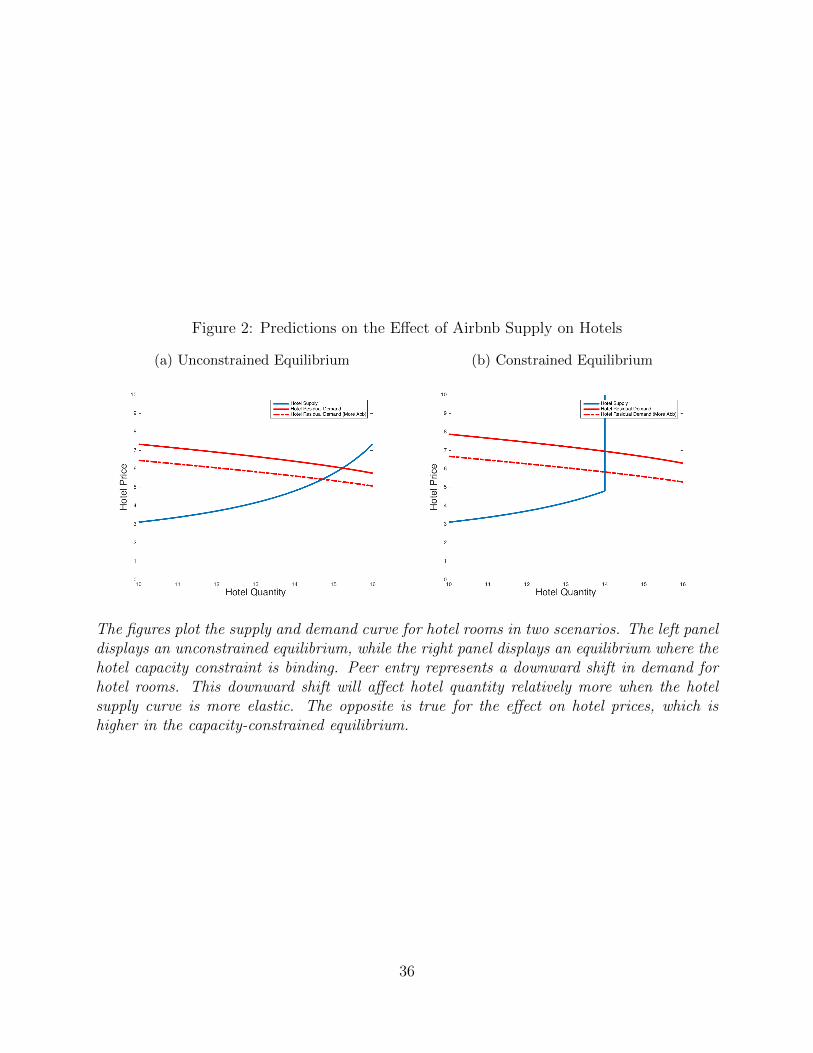
Figure 2: Predictions on the Effect of Airbnb Supply on Hotels

(a) Unconstrained Equilibrium (b) Constrained Equilibrium

The figures plot the supply and demand curve for hotel rooms in two scenarios. The left paneldisplays an unconstrained equilibrium, while the right panel displays an equilibrium where thehotel capacity constraint is binding. Peer entry represents a downward shift in demand forhotel rooms. This downward shift will affect hotel quantity relatively more when the hotelsupply curve is more elastic. The opposite is true for the effect on hotel prices, which ishigher in the capacity-constrained equilibrium.

36

Figure 3: Peer Production and Hotel Revenues

This figure plots the supply share of Airbnb against the average revenue per available roomin each respective city.

37

Figure 4: Peer Production and Fixed or Marginal Costs

(a) Hotel Supply Constraints (b) Peers’ Marginal Costs

The figures plot the size of Airbnb against a proxy for hotel investment costs (left panel) and aproxy for peers’ marginal costs (right panel). The proxy for the constraints to the constructionof new hotels is the share of undevelopable area developed by Saiz. This index measures theshare of a city that is undevelopable due to geographic constraints, like steep mountains orthe ocean. The proxy for peers’ marginal costs is the share of unmarried adults in the MSA.The size of Airbnb is measured as the average share of available listings in the last quarter of2014. Figure A2 in the Appendix confirms that other proxies such as regulatory constraints,the share of children, and the rent to income ratio are also good predictors of peer entry.

38

Figure 5: Peer Production and Demand Characteristics

(a) Demand Growth (b) Demand Variability

The figures plot the size of Airbnb against the growth rate in incoming air passengers toan MSA between June 2011 and June 2012 (left) and against the standard deviation ofincoming air passengers (right). The standard deviation of air travelers is measured using2011 monthly data on arriving (not returning) passengers at major US airports. We focuson data from 2011-2012, when Airbnb was very small relative to the accommodation market,to limit the possibility that the availability of Airbnb hosts could generate such growth orvariability in demand. The size of Airbnb is measured as the average share of availablelistings in the last quarter of 2014.

39

Figure 6: Measures of Airbnb Supply: Demand-induced Calendar Updates

Booked Listings

Available Listings(Unadjusted)

Available Listings

Active Listings

25

50

75

100

2012 2013 2014 2015Date

Size

of A

irbnb

(Lin

ear S

cale

)

This figure plots four measures of the size of Airbnb. An active listings is defined as a listingavailable to be booked or booked for any future date. An (unadjusted) available listing isone that is either booked or has an open calendar slot on the date of stay. Available listingsaugment the unadjusted measure with listings that were contacted and updated their calendarsto be unavailable prior to the date of stay. A booked listing is one that has been booked forthat date.

40

Figure 7: Prices and Occupancy Rates

This figure plots prices and occupancy rates of upscale hotels in New York in 2014.

41

Figure 8: Estimated Utilities for Accommodation Options Across Cities

This figure plots the estimated mean utilities for accommodation options across the 10 citiesused in our estimation. The values are computed as averages over the last month in ourdata. The negative values of some of the parameters reflect the fact that our normalizationof the outside option means that most people choose the outside option.

42

Figure 9: Estimated Hotel Costs

(a) Costs by City – Midscale Hotels (b) Costs by Hotel Scale – New York City

This figure plots the estimated marginal cost curves of hotels across cities (left panel) andacross scales (right panel). The values are computed as averages over the last month in ourdata. Appendix Tables A6 and A7 display the cost estimates by city and hotel scale.

43

Figure 10: Mean Costs of Airbnb Hosts in New York City

The figures plot the estimated mean costs of Airbnb hosts in New York over time.

44

Tables

Table 1: Descriptive Statistics on Hotel and Airbnb Outcomes

Statistic N Mean St. Dev. Pctl(25) Median Pctl(75)

Mean Hotel Occupancy 50 0.66 0.07 0.61 0.65 0.70Std Dev Hotel Occupancy 50 0.13 0.03 0.12 0.14 0.15Mean Hotel Price in $ 50 107.94 35.04 86.29 98.69 121.01Std Dev Hotel Price 50 16.34 9.34 9.77 13.00 21.02Mean Hotel Revenue (Thousand $) 50 3,785.34 3,588.86 1,575.12 2,488.65 4,856.56Airbnb Share of Available Rooms (Q4 2014) 50 0.02 0.03 0.005 0.01 0.03Airbnb Share of Potential Guests (Q4 2014) 50 0.04 0.04 0.01 0.02 0.05Airbnb Share of Housing Units (Q4 2014) 50 0.001 0.001 0.0002 0.0005 0.001Mean Airbnb Occupancy 50 0.15 0.06 0.11 0.13 0.18Std Dev Airbnb Occupancy 50 0.09 0.02 0.07 0.08 0.10Mean Airbnb Price in $ 50 108.63 24.67 92.01 99.76 120.87Std Dev Airbnb Price 50 31.24 13.17 21.78 28.50 34.29Mean Airbnb to Hotel Price Ratio 50 1.06 0.28 0.91 1.00 1.14Std Dev Price Ratio 50 0.33 0.18 0.21 0.29 0.39

This table shows hotel and Airbnb descriptive statistics for the 50 cities in our sample. For each city, we compute the meanand standard deviation of daily occupancy rate and price for hotels and Airbnb listings. The Airbnb share of available roomsis computed as the average of daily share of rooms in the last quarter, i.e. October - December 2014. The Airbnb share ofpotential guests is computed as the quarterly average of rooms adjusted for their realized capacity, assuming that the typicalhotel has the same number of average guests as a ’Midscale’ Airbnb listing. This number is larger than the Airbnb share ofrooms because Airbnb listings typically have higher capacity than hotel rooms.

Table 2: Descriptive Statistics on Market Characteristics

Statistic N Mean St. Dev. Pctl(25) Median Pctl(75)

WRLURI 50 0.31 0.82 −0.30 0.20 0.84Share of Undevelopable Area 46 0.30 0.24 0.09 0.23 0.43Percent Never Married 48 0.33 0.03 0.31 0.33 0.36Share of Children 48 0.31 0.02 0.30 0.31 0.32Rent to Income Ratio 50 0.18 0.03 0.15 0.17 0.20Std Dev of Google Trend (2011) 50 12.05 4.22 9.62 11.51 13.70Std Dev of Incoming Passengers (2011) / 10,000 50 6.95 6.63 1.89 4.17 11.30Passengers’ Growth (2012-2011) 50 0.02 0.06 −0.02 0.01 0.04

The table shows descriptive statistics on market characteristics for the 50 cities in our sample. The WRLURI and Saiz’s shareof undevelopable area are proxies for constraints to hotel supply. The share of children and unmarried adults proxy for theavailability of Airbnb hosts. The standard deviation of Google trends and incoming passengers are two measures of demandvolatility.

45

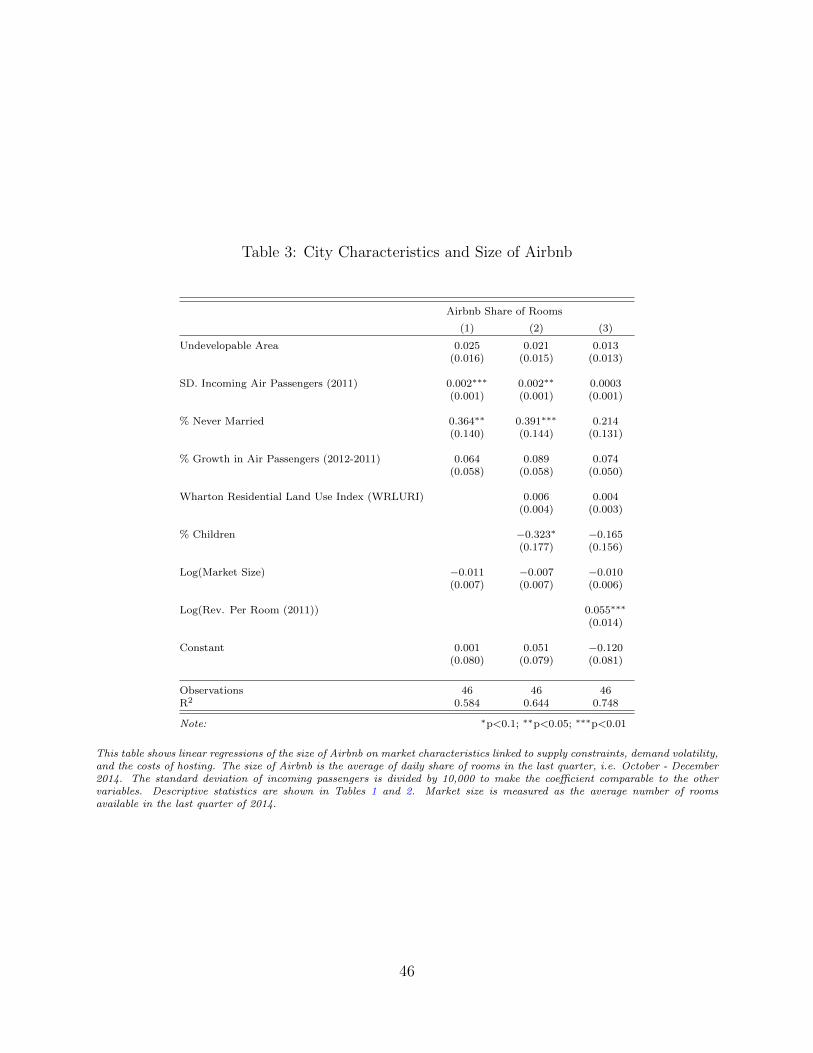
Table 3: City Characteristics and Size of Airbnb

Airbnb Share of Rooms

(1) (2) (3)

Undevelopable Area 0.025 0.021 0.013(0.016) (0.015) (0.013)

SD. Incoming Air Passengers (2011) 0.002∗∗∗ 0.002∗∗ 0.0003(0.001) (0.001) (0.001)

% Never Married 0.364∗∗ 0.391∗∗∗ 0.214(0.140) (0.144) (0.131)

% Growth in Air Passengers (2012-2011) 0.064 0.089 0.074(0.058) (0.058) (0.050)

Wharton Residential Land Use Index (WRLURI) 0.006 0.004(0.004) (0.003)

% Children −0.323∗ −0.165(0.177) (0.156)

Log(Market Size) −0.011 −0.007 −0.010(0.007) (0.007) (0.006)

Log(Rev. Per Room (2011)) 0.055∗∗∗

(0.014)

Constant 0.001 0.051 −0.120(0.080) (0.079) (0.081)

Observations 46 46 46R2 0.584 0.644 0.748

Note: ∗p<0.1; ∗∗p<0.05; ∗∗∗p<0.01

This table shows linear regressions of the size of Airbnb on market characteristics linked to supply constraints, demand volatility,and the costs of hosting. The size of Airbnb is the average of daily share of rooms in the last quarter, i.e. October - December2014. The standard deviation of incoming passengers is divided by 10,000 to make the coefficient comparable to the othervariables. Descriptive statistics are shown in Tables 1 and 2. Market size is measured as the average number of roomsavailable in the last quarter of 2014.

46

Table 4: The Supply Elasticity of Hotels and Peer Hosts

Log(Hotel Rooms Boooked) Log(Airbnb Rooms Booked)

(1) (2)

log(Hotel Rooms) 0.538∗∗∗

(0.188)

log(Hotel Price) 1.072∗∗∗

(0.069)

log(Airbnb Rooms) 0.622∗∗∗

(0.098)

log(Airbnb Price) 2.164∗∗∗

(0.296)

IV Yes YesCity FE Yes YesYear-Month FE Yes YesDay of Week FE Yes YesObservations 268,489 250,923R2 0.963 0.895

Note: Column 2 includes the log number of residents leaving by air,and the log number of outgoing travel searches on Google as controls.

Standard Errors are clustered at the city and year-month level.

The table shows results of IV regressions of the log of hotel and Airbnb bookings on the corresponding price and room availability.Column 2 includes the log of departing (local) air travelers, and the one week lag of the log of local Google Search Trends forhotels outside of the city as additional controls. The instruments are demand-side shifters – the one week lag of the log ofthe Google Search Trends and the log of arriving (not returning) flight travelers – in both columns. In column 2 the numberof Airbnb available listings is instrumented with city-specific quadratic time trends that capture the diffusion process of theplatform. Adding the city-day observations with no Airbnb bookings (and using hotel prices in column 2) does not change theresults. Instrumenting for hotel capacity like we do for Airbnb does not change the results either.

47

Table 5: Hotel Revenue and the Size of Airbnb

Log(RevPAR) Occupancy Rate Log(Price)

(1) (2) (3)

log(Incoming Air Passengers) 1.169∗∗∗ 0.394∗∗∗ 0.498∗∗∗

(0.065) (0.041) (0.041)

log(Google Search Trend) 0.147∗∗∗ 0.054∗∗∗ 0.069∗∗

(0.049) (0.012) (0.027)

log(Hotel Rooms) −0.768∗∗∗ −0.436∗∗∗ −0.078(0.200) (0.078) (0.148)

log(Available Listings) −0.033∗∗ −0.006 −0.025∗

(0.014) (0.005) (0.013)

IV Yes Yes YesCity FE Yes Yes YesYear-Quarter FE Yes Yes YesDay of Week FE Yes Yes YesObservations 268,489 268,489 268,489R2 0.729 0.582 0.853

Note: Standard Errors Clustered at a City Level

This table shows results of IV estimates of equation 4, where the size of Airbnb is measured as the number of available listings.The Google search trend is a one-week lag. The instruments are city-specific quadratic time trends. The dependent variableis revenue per available room in column 1, occupancy rate in column 2, and price in column 3. Appendix B discusses theinstrumental variables strategy and endogeneity concerns in greater detail.

48

Tab

le6:

Het

erog

eneo

us

Eff

ects

ofA

irbnb:

Mar

ket

Supply

Ela

stic

ity

Log(R

evP

AR

)O

ccu

pan

cyR

ate

Log(P

rice

)L

og(R

evP

AR

)O

ccu

pan

cyR

ate

Log(P

rice

)

(1)

(2)

(3)

(4)

(5)

(6)

log(I

nco

min

gA

irP

ass

enger

s)1.1

38∗∗∗

0.4

11∗∗∗

0.5

28∗∗∗

1.2

83∗∗∗

0.4

97∗∗∗

0.4

40∗∗∗

(0.1

10)

(0.0

31)

(0.0

69)

(0.1

28)

(0.0

34)

(0.0

82)

log(G

oogle

Sea

rch

Tre

nd

)0.1

51∗

0.0

43∗∗

0.0

81∗

0.1

17

0.0

66∗∗

0.0

26

(0.0

91)

(0.0

21)

(0.0

47)

(0.0

72)

(0.0

26)

(0.0

26)

log(H

ote

lR

oom

s)−

0.7

17

−0.3

59∗∗∗

−0.2

71

−0.9

92∗∗

−0.5

42∗∗∗

−0.0

02

(0.4

70)

(0.0

67)

(0.3

88)

(0.3

89)

(0.1

73)

(0.2

11)

log(A

vailab

leL

isti

ngs)

−0.0

70

−0.0

09

−0.0

60∗∗

−0.0

06

−0.0

07

0.0

08

(0.0

49)

(0.0

07)

(0.0

28)

(0.0

55)

(0.0

20)

(0.0

24)

Cit

yT

yp

eIn

elast

icH

ou

sin

gS

up

ply

Ela

stic

Hou

sin

gS

up

ply

Inst

rum

ents

Yes

Yes

Yes

Yes

Yes

Yes

Cit

yF

EY

esY

esY

esY

esY

esY

esY

ear-

Qu

art

erF

EY

esY

esY

esY

esY

esY

esD

ay

of

Wee

kF

EY

esY

esY

esY

esY

esY

esO

bse

rvati

on

s112,3

48

112,3

48

112,3

48

134,8

01

134,8

01

134,8

01

R2

0.7

41

0.5

97

0.8

52

0.5

47

0.5

07

0.7

01

No

te:

Sta

nd

ard

Err

ors

Clu

ster

edat

aC

ity

an

dY

ear-

Qu

art

erL

evel

Th

eta

ble

sho

ws

resu

lts

of

IVes

tim

ate

ssi

mil

ar

toT

abl

e5

,bu

tw

esp

lit

the

citi

esby

the

ho

usi

ng

sup

ply

ela

stic

ity

esti

ma

ted

inS

aiz

(20

10

).In

ela

stic

citi

esa

reth

ose

wit

ha

ho

usi

ng

sup

ply

ela

stic

ity

belo

wth

em

edia

na

cro

sso

ur

sam

ple

.

49

Table 7: Selected Estimated Parameters

Parameter Value Std. Error

Price -0.014 0.003Time Trend 0.002 0.001Time Trend * Airbnb 0.010 0.001Log Google Trend 2.952 2.161Log Google Trend Sq. -0.175 0.248Log Travelers To 5.563 0.615Log Travelers To Sq. -0.150 0.000Std. Deviation on Inside Option 1.074 0.396Std. Deviation on Hotel Class 0.354 0.223

This table displays the estimated parameters and their standard errors for selected parameters in the model.

50

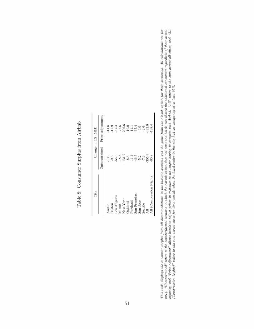
Tab

le8:

Con

sum

erSurp

lus

from

Air

bnb

Cit

yC

han

ge

inC

S(M

M)

Un

con

stra

ined

Pri

ceA

dju

stm

ent

Au

stin

-10.9

-14.6

Bost

on

-9.5

-12.9

Los

An

gel

es-5

6.5

-67.4

Mia

mi

-18.8

-23.6

New

York

-131.2

-206.6

Oakla

nd

-8.3

-10.0

Port

lan

d-1

1.7

-14.1

San

Fra

nci

sco

-46.5

-67.4

San

Jose

-5.2

-6.0

Sea

ttle

-7.3

-9.6

All

-305.9

-432.0

All

(Com

pre

ssio

nN

ights

)-8

0.8

-138.4

Th

ista

ble

dis

pla

ys

the

con

sum

ersu

rplu

sfr

om

all

acc

om

mod

ati

on

sin

the

base

lin

esc

ena

rio

an

dth

ega

ins

fro

mth

eA

irbn

bo

pti

on

for

thre

esc

ena

rio

s.A

llca

lcu

lati

on

sa

refo

r2

01

4.

“U

nco

nst

rain

ed”

refe

rsto

the

cou

nte

rfa

ctu

al

scen

ari

oin

wh

ich

the

Air

bnb

op

tio

nd

oes

no

tex

ist

an

dh

ote

lsca

na

bso

rbth

ea

dd

itio

na

lco

nsu

mer

sre

gard

less

of

thei

ra

ctu

al

capa

city

,a

nd

“P

rice

Ad

just

men

t”a

llo

ws

ho

tels

toa

dju

stp

rice

sin

resp

on

seto

no

lon

ger

ha

vin

gto

com

pete

wit

hA

irbn

b.“

All

”re

fers

toth

esu

ma

cro

ssa

llci

ties

,a

nd

“A

ll(C

om

pre

ssio

nN

igh

ts)”

refe

rsto

the

sum

acr

oss

citi

esfo

rti

me

peri

ods

wh

enth

eh

ote

lse

cto

rin

the

city

ha

da

noc

cupa

ncy

of

at

lea

st9

5%

.

51

Tab

le9:

Con

sum

erSurp

lus

from

Air

bnb

(per

nig

ht)

Cit

yA

vg.

Air

bnb

Pri

ceC

on

sum

erS

urp

lus

per

Per

son

-Nig

ht

Un

con

stra

ined

Pri

ceA

dju

stm

ent

Au

stin

160.6

-52.8

-70.7

Bost

on

136.2

-60.8

-82.3

Los

An

gel

es124.6

-55.3

-66.0

Mia

mi

155.0

-61.1

-76.5

New

York

145.3

-43.8

-68.9

Oakla

nd

89.4

-60.2

-72.7

Port

lan

d99.4

-64.9

-78.2

San

Fra

nci

sco

146.6

-47.1

-68.1

San

Jose

113.4

-63.6

-73.8

Sea

ttle

120.0

-66.3

-86.3

All

139.4

-49.4

-69.8

All

(Com

pre

ssio

nN

ights

)147.1

-50.0

-85.6

Th

ista

ble

dis

pla

ys

the

con

sum

ersu

rplu

spe

rn

igh

tbo

oke

dfr

om

the

Air

bnb

op

tio

nfo

rth

ree

cou

nte

rfa

ctu

al

scen

ari

os.

All

calc

ula

tio

ns

are

for

20

14

.“

Un

con

stra

ined

”re

fers

toth

eco

un

terf

act

ua

lsc

ena

rio

inw

hic

hth

eA

irbn

bo

pti

on

doe

sn

ot

exis

ta

nd

ho

tels

can

abs

orb

the

ad

dit

ion

al

con

sum

ers

rega

rdle

sso

fth

eir

act

ua

lca

paci

ty,

an

d“

Pri

ceA

dju

stm

ent”

all

ow

sh

ote

lsto

ad

just

pri

ces

inre

spo

nse

ton

olo

nge

rh

avi

ng

toco

mpe

tew

ith

Air

bnb.

“A

ll”

refe

rsto

the

sum

acr

oss

all

citi

es,

an

d“

All

(Co

mp

ress

ion

Nig

hts

)”re

fers

toth

esu

ma

cro

ssci

ties

for

tim

epe

riod

sw

hen

the

ho

tel

sect

or

inth

eci

tyh

ad

an

occu

pan

cyo

fa

tle

ast

95

%.

52

Tab

le10

:C

omp

etit

ive

Eff

ects

onH

otel

s

Cit

y%

Ch

an

ge

Qu

anti

ty%

Ch

an

ge

Rev

enu

e%

Ch

an

ge

Pro

fit

Un

con

st.

Pri

ceA

dj.

Un

con

st.

Pri

ceA

dj.

Un

con

st.

Pri

ceA

dj.

Au

stin

0.6

80.4

30.8

90.7

51.3

41.9

6B

ost

on

0.3

60.2

10.4

00.3

10.5

10.7

7L

os

An

gel

es1.0

30.7

71.1

81.0

11.5

14.4

0M

iam

i0.7

10.5

00.8

40.7

01.1

51.2

2N

ewY

ork

2.2

20.7

52.4

51.5

02.6

74.0

9O

akla

nd

0.7

40.5

40.8

10.7

70.9

62.7

1P

ort

lan

d0.8

50.6

30.9

50.8

81.2

43.0

1S

an

Fra

nci

sco

1.5

90.7

21.7

31.2

31.8

24.0

4S

an

Jose

0.2

70.2

20.2

80.2

60.2

80.6

5S

eatt

le0.3

30.2

10.3

80.3

20.5

21.0

5A

ll1.1

20.5

71.4

41.0

01.8

13.0

5A

ll(C

om

pre

ssio

n)

1.4

00.3

01.7

60.9

71.9

12.5

0

Th

ista

ble

dis

pla

ys

ho

tel

boo

kin

gsa

nd

reve

nu

ea

cro

ssco

un

terf

act

ua

lsc

ena

rio

s.A

llca

lcu

lati

on

sa

refo

r2

01

4.

“B

ase

”re

fers

toth

ea

ctu

al

da

ta,

“U

nco

nst

.”re

fers

toth

eco

un

terf

act

ua

lsc

ena

rio

inw

hic

hth

eA

irbn

bo

pti

on

doe

sn

ot

exis

ta

nd

ho

tels

can

abs

orb

the

ad

dit

ion

al

con

sum

ers

rega

rdle

sso

fth

eir

act

ua

lca

paci

ty,

an

d“

Pri

ceA

dj.

”re

fers

toth

eco

un

terf

act

ua

lw

her

eh

ote

lsa

dju

stp

rice

sin

resp

on

seto

no

lon

ger

ha

vin

gto

com

pete

wit

hA

irbn

b.R

ow

“A

ll”

refe

rsto

the

sum

acr

oss

all

citi

es,

an

dro

w“

All

(Co

mp

ress

ion

)”re

fers

toth

esu

ma

cro

ssci

ties

for

tim

epe

riod

sw

hen

the

ho

tel

sect

or

inth

eci

tyh

ad

an

occu

pan

cyo

fa

tle

ast

95

%.

53

Table 11: Airbnb Bookings: Market Expansion versus Business Stealing

Share New BookingsUnconstr. Price Adjust.

Austin 0.62 0.76Boston 0.61 0.78Los Angeles 0.62 0.72Miami 0.61 0.72New York 0.59 0.86Oakland 0.64 0.74Portland 0.63 0.73San Francisco 0.60 0.82San Jose 0.64 0.71Seattle 0.63 0.77

This table shows the number of rooms booked on Airbnb by city and year according to our model estimates. “Unconstr.” refers tothe counterfactual scenario in which the Airbnb option does not exist and hotels can absorb the additional consumers regardlessof their actual capacity, “Cap Constr.” imposes hotel capacity constraints, and “Price Adjust.” reflects the counterfactualwhere Airbnb is removed and hotels adjust prices.

Table 12: Peer Producer Surplus

City Avg. Peer Surplus per Night Total Peer Surplus (MM)

Austin 30.86 1.17Boston 26.87 0.99Los Angeles 25.99 3.30Miami 24.36 1.10New York 28.07 7.90Oakland 25.50 0.50Portland 28.65 0.95San Francisco 28.79 2.90San Jose 27.47 0.52Seattle 27.58 0.90All 27.58 20.23All (Compression Nights) 28.82 8.98

This table displays the peer producer surplus for 2014. Row “All” refers to the sum across all cities, and row “All (Com-pression)” refers to the sum across cities for time periods when the hotel sector in the city had an occupancy of at least95%.

54

A Appendix: Proof of Model Predictions

The short-run model from section 2.1 offers some comparative statics predictions. We present

the propositions and the proofs below.

Proposition 1 Hotel profits and prices decrease in Ka. Hotel rooms sold decrease in Ka if

and only if − ∂Qh∂pa/∂Qh∂ph≥ − ∂2Πh

∂ph∂pa/∂

2Πh

∂p2h

.

Before we start the proof of Proposition 1 it is useful to separately consider markets where

the hotel capacity constraint binds and markets where it does not. In markets where the

hotel constraint binds the two equilibrium conditions are Qh(ph, pa) = Kh and Qa(pa, ph) =

KaG(pa), where G() denotes the distribution of flexible marginal costs. See Section 2.1

for details. By totally differentiating the system of equilibrium equations we find the total

derivatives of hotel and Airbnb prices with respect to Airbnb capacity:

[dphdKa

]c=

−∂Qh∂pa

G(pa)

∂Qh∂ph

[∂Qa∂pa−Kag(pa)

]− ∂Qh

∂pa

∂Qa∂ph

(A1)

[dpadKa

]c=

∂Qh∂ph

G(pa)

∂Qh∂ph

[∂Qa∂pa−Kag(pa)

]− ∂Qh

∂pa

∂Qa∂ph

. (A2)

In markets where the hotel constraint does not bind the two equilibrium conditions

are ∂Π(pa, ph)/∂ph = 0 and Qa(pa, ph) = KaG(pa). By totally differentiating the system of

equilibrium equations we find the total derivatives of hotel and Airbnb prices with respect

to Airbnb capacity:

[dphdKa

]u=

− ∂2Πh∂ph∂pa

G(pa)

∂2Πh∂p2h

[∂Qa∂pa−Kag(pa)

]− ∂2Πh

∂ph∂pa

∂Qa∂ph

(A3)

[dpadKa

]u=

∂2Πh∂p2hG(pa)

∂2Πh∂p2h

[∂Qa∂pa−Kag(pa)

]− ∂2Πh

∂ph∂pa

∂Qa∂ph

, (A4)

where ∂2Πh∂p2h

= 2∂Qh∂ph

+ ∂2Qh∂p2h

(ph − ch), and ∂2Πh∂ph∂pa

=[∂Qh∂pa

+ ∂2Qh∂ph∂pa

(ph − ch)].

We start by proving that hotel prices are a decreasing function of flexible capacity in both

constrained and unconstrained equilibria. To do that, we need to prove that the derivatives

in equation A1 and A3 are negative.[dphdKa

]c≤ 0 since the numerator is negative and the

denominator is positive. The numerator is negative as long as hotels and Airbnb rooms are

substitutes, or ∂Qh∂pa≥ 0. The denominator is positive because the first term is the product

of two negative terms, and the second term to be substracted is positive but smaller than55

the first term in absolute value. Indeed, −∂Qa∂pa

+ Kag(pa) ≥ ∂Qh∂pa≥ 0 and −∂Qh

∂ph≥ ∂Qa

∂phsince

own-price elasticities are negative, cross-price elasticities are positive, and as long as there

is an outside good with positive demand Q0, −∂Qj∂pj

= ∂Qi∂pj

+ ∂Q0

∂pj≥ ∂Qi

∂pj.

A similar reasoning proves that[dphdKa

]u≤ 0. The inequality holds as long as the Bertrand

price equilibrium is stable and hotel optimal prices are an increasing function of competitors’

prices (Bulow et al. (1985)). The conditions on the stability of equilibrium and strategic

complementarity in prices imply that −∂2Πh∂p2h≥ ∂2Πh

∂ph∂pa≥ 0 , or −

[2∂Qh∂ph

+ ∂2Qh∂p2h

(ph − ch)]≥[

∂Qh∂pa

+ ∂2Qh∂ph∂pa

(ph − ch)]≥ 0.

So far, we have proved that an increase in flexible capacity decreases hotel prices by

showing that dphdKa≤ 0 whether or not the hotel is operating at capacity.

Now we prove that an increase in flexible capacity also decreases hotel profits in both

constrained and unconstrained equilibria. An increase in Ka affects hotel profits Πh =

Qdh(ph − ch) through changes in pa and ph:

dΠh

dKa

=∂Πh

∂ph

dphdKa

+∂Πh

∂pa

dpadKa

. (A5)

Let us first consider the case where the hotel capacity constraint binds, and the price

derivatives with respect to Ka are given by equations A1 and A2. Since we are at a con-

strained maximum ∂Πh∂ph

= ∂Qh∂ph

(ph−ch)+Qh < 0. Since hotel and Airbnb rooms are substitutes∂Πh∂pa

= ∂Qh∂pa

(ph − ch) ≥ 0. After substituting the expressions of ∂Πh∂ph

and ∂Πh∂pa

, and equations

A1 and A2 into equation A5, simple algebra shows that equation A5 is negative if and only

if −Qh∂Qh∂pa

G(pa) ≤ 0, which is always true.

Let us now consider the case where the hotel capacity constraint does not bind. At

the unconstrained optimum the first order condition holds with equality, ∂Πh∂ph

= 0, so the

first term in equation A5 is zero. The second term has the same sign as[dpadKa

]u≤ 0.

From equation A4, this derivative is negative because it has the same sign as ∂2Πh∂p2h

. The

last expression is the second derivative of the hotel profit optimization function, which is

negative for an interior maximum. Combining these results implies that flexible prices are

a decreasing function of flexible capacity even when hotels are not capacity constrained in

equilibrium. Therefore, whether the hotel is operating at capacity or not, dΠhdKa≤ 0: an

increase in flexible capacity reduces hotel profits.

We are left with proving that hotel rooms sold decrease in Ka if and only if − ∂Qh∂pa/∂Qh∂ph≥

− ∂2Πh∂ph∂pa

/∂2Πh

∂p2h

. In words, this condition requires that the hotel best response function to

competitor prices is steeper when hotel occupancy is held fixed than when hotel occupancy

56

is allowed to change.16 The total derivative of hotel rooms sold with respect to Airbnb

capacity is equal todQh

dKa

=∂Qh

∂ph

dphdKa

+∂Qh

∂pa

dpadKa

. (A6)

When hotels are operating at capacity a marginal change in Airbnb capacity does not change

hotel occupancy. Indeed, substituting equations A1 and A2 gives[dQhdKa

]c= 0. When

hotels are not operating at capacity, substituting equations A3 and A4 gives[dQhdKa

]c=

− ∂Qh∂ph

∂2Πh∂ph∂pa

G(pa)+∂Qh∂pa

∂2Πh∂p2h

G(pa)

∂2Πh∂p2h

[ ∂Qa∂pa−Kag(pa)]− ∂2Πh

∂ph∂pa

∂Qa∂ph

. We have already proved that the denominator is positive,

while the numerator is negative as long as −∂Qh∂ph

∂2Πh∂ph∂pa

+ ∂Qh∂pa

∂2Πh∂p2h≤ 0, which is identical

to the condition stated in the proposition. �

Proposition 2 The reduction in hotel prices when flexible capacity increases is larger when

hotel capacity constraints bind if and only if − ∂Qh∂pa/∂Qh∂ph≥ − ∂2Πh

∂ph∂pa/∂

2Πh

∂p2h

. Under the same

condition, the reduction in hotel rooms sold when flexible capacity increases is larger when

hotel capacity constraints do not bind.

To prove that hotel prices fall more as a function of flexible capacity when hotel capacity

constraints bind, it suffices to show that equation A1 is smaller than equation A3. In proving

proposition 1 we have showed that both derivatives are negative. After some algebra, the

condition[dphdKa

]c≤[dphdKa

]usimplifies to − ∂Qh

∂pa/∂Qh∂ph≥ − ∂2Πh

∂ph∂pa/∂

2Πh

∂p2h

.

To prove that hotel rooms sold fall more as a function of flexible capacity when hotel

capacity constraints do not bind, we again use parts of the proof of Proposition 1. There, we

have showed that hotel rooms sold are unchanged following a marginal increase in flexible

capacity whenever hotel constraints bind:[dQhdKa

]c= 0. We have also showed that

[dQhdKa

]u≤ 0

if and only if − ∂Qh∂pa/∂Qh∂ph≥ − ∂2Πh

∂ph∂pa/∂

2Πh

∂p2h

. Therefore[dQhdKa

]u≤[dQhdKa

]c. �

The next proposition contains comparative statics results on the long-run entry of peer

supply. Throughout, we assume that all flexible suppliers with joining costs lower than C,

where C = va =∫dEc(max{0, pda − c}

)dF (d) have already joined. This corresponds to mass

Ka.

Proposition 3 Entry of flexible sellers is larger (Ka increases) if the distribution of peers’

marginal costs c decreases in the sense of first-order stochastic dominance. Ka increases

16− ∂Qh∂pa

/∂Qh∂ph

is the partial derivative of hotel prices with respect to Airbnb prices computed by implicit

function theorem on the constrained equilibrium condition, Qh(ph, pa) = Kh. Analogously, − ∂2Πh∂ph∂pa

/∂2Πh∂p2

h

is

the partial derivative under the unconstrained equilibrium condition, ∂Πh(ph, pa)/∂ph = 0.

57

if Kh decreases. Ka also increases if F (d) increases in the sense of first order stochastic

dominance or in response to a mean-preserving spread in F (d).

It is intuitive that if the distribution of flexible marginal costs c shifts to the left,

Ec[max{0, pda − c}

]weakly increases in every demand state, so va increases and more flexible

sellers enter.

It is also straightforward to see that if F (d) shifts to the right, Ec[max{0, pda − c}

]will

not change for any demand state, but higher demand states are more likely so va increases,

inducing more flexible entry.

Proving that a reduction in Kh induces more flexible entry requires a little more explana-

tion. Assume Kh decreases on the margin. For demand states for which Kh was not binding,

the decrease in hotel capacity has no effect, so pda does not change for d lower than a certain

threshold. For demand states in which Kh was binding the two equilibrium conditions are,

with simplified notation, Qdh(ph, pa) = Kh and Qd

a(pa, ph) = KaG(pa). We proved above (for

Propositions 1 and 2) that an increase in flexible capacity decreases both hotel and peer

prices. An analogous proof is valid for a change in hotel capacity. So for high demand states

a decrease in hotel capacity increases flexible prices. So far we showed that in unconstrained

demand states flexible prices do not change if Kh decreases, while in constrained demand

states they increase. This is a shift in the distribution of flexible prices in the sense of first

order stochastic dominance. So dvadKh≤ 0 and a decrease in hotel capacity induces more

flexible entry.

Finally, a mean-preserving spread of F (d) induces more entry of flexible sellers. The

utility function for demand state d, Ec[max{0, pda − c}

], is a convex function of pda. Since

pda is an increasing function of d, as long as it is not too concave, the result is a direct

implication of Jensen’s inequality. Intuitively, flexible sellers lose nothing from low demand

periods since they can choose not to host, and gain high profits in periods of high demand.

A sufficient condition for this to hold is that flexible prices are non-decreasing in d, which

is the case if hotel and flexible prices are strategic complements and the Bertrand price

equilibrium is stable. As before, the proof relies on totally differentiating the system of

equilibrium equations Qda = KaG(pa) and Qd

h = −∂Qdh∂ph

(ph − ch) (which is Qdh = Kh if hotels

are capacity-constrained) with respect to the demand state and the price variables. The

sufficient conditions require that − ∂2Πdh

∂ph∂pa/∂

2Πdh

∂p2h

∈ (0, 1) (equilibrium stability and strategic

complementarity of hotel and flexible prices) and − ∂2Πdh

∂ph∂d/∂

2Πdh

∂p2h

≥ 0 (optimal hotel price is

an increasing function of demand), where ∂Πdh/∂ph is the first order condition of the hotel

maximization problem. �

58

B Appendix: Endogeneity Concerns

This Appendix presents evidence validating our baseline specification in equation 4 against

endogeneity concerns. First, in Table A1 we progressively add controls from a simple re-

gression of hotel revenue on the size of Airbnb. Our baseline specification in OLS form is in

the fifth column. The coefficients of Airbnb listings decreases as we keep adding controls for

demand fluctuations, days of the weeks, seasonality, and market-specific characteristics.

Appendix Table A2 displays OLS results using specification 4 for four different measures

of Airbnb size: active, available (the naive version), adjusted available, and booked Airbnb

rooms. This table shows the flaws related to each potential measure of Airbnb size. A

regression using active listings, displayed in Column (1), results in a negative, but small

effect. Column (2) displays results using the naive measure of available listings. In this

case, the OLS estimate is much larger in magnitude than our IV estimates. The reason for

this, as previously described, is that this variable is counter-cyclical: hosts are more likely

to update their unavailability on their calendar in periods of high demand, meaning that

measured supply is negatively correlated with demand. Column (3) displays our preferred

measure of availability described in the previous section. The OLS estimate is not significant

and smaller in magnitude than the IV estimate, which is expected if there is bias due to the

number of available listings being positively correlated with demand. Lastly, Column (4)

shows the results with respect to the number of Airbnb bookings. There is a positive and

statistically significant coefficient because demand for Airbnb is highest precisely in times of

high overall accommodations demand, as shown in the previous subsection.

Appendix Table A3 displays the full set of results described in the previous paragraph

but with the measure of Airbnb instrumented with city-specific quadratic time trends. Using

this strategy, the effect of Airbnb is similar regardless of the measure used, except for booked

listings.

59

Table A1: Hotel Revenue and Airbnb - Additional Controls

Log(Revenue per Available Hotel Room)

(1) (2) (3) (4) (5)

log(Available Listings) 0.177∗∗∗ 0.124∗∗∗ 0.125∗∗∗ 0.043∗∗∗ −0.032(0.019) (0.016) (0.016) (0.005) (0.021)

log(Google Search Trend) 0.388∗∗∗ 0.388∗∗∗ 0.311∗∗∗ 0.147∗∗∗

(0.060) (0.060) (0.037) (0.049)

log(Incoming Air Passengers) 0.181∗∗∗ 0.180∗∗∗ 1.016∗∗∗ 1.169∗∗∗

(0.041) (0.041) (0.047) (0.065)

log(Hotel Rooms) −0.166∗ −0.166∗ −0.444∗ −0.767∗∗∗

(0.099) (0.099) (0.254) (0.198)

Day of Week FE No No Yes Yes YesCity FE No No No Yes YesQuarter-Year FE No No No No YesObservations 268,489 268,489 268,489 268,489 268,489R2 0.325 0.445 0.504 0.717 0.729

Note: Standard Errors Clustered at a City Level

The table shows OLS estimates of equation 4. It progressively add controls: day of the week fixed effects, month fixed effects(January 2011 is a different fixed effect from January 2012), market fixed effects (e.g. SF), and city-specific time trends.The first columns show clearly a spurious correlation: Airbnb grows in markets where the accommodation industry is thriving.With the inclusion of additional controls the effect of Airbnb is negative across the markets under consideration.

60

Table A2: Hotel Revenue and Airbnb - Different Measures of Airbnb

Log(Revenue per Available Hotel Room)

(1) (2) (3) (4)

log(Active Listings) −0.015(0.013)

log(Available Listings Raw) −0.101∗∗∗

(0.027)

log(Available Listings Corrected) −0.032(0.021)

log(Booked Listings) 0.139∗∗∗

(0.013)

log(Google Search Trend) 0.147∗∗∗ 0.145∗∗∗ 0.147∗∗∗ 0.122∗∗∗

(0.050) (0.049) (0.049) (0.047)

log(Incoming Air Passengers) 1.171∗∗∗ 1.149∗∗∗ 1.169∗∗∗ 0.961∗∗∗

(0.065) (0.063) (0.065) (0.056)

log(Hotel Rooms) −0.758∗∗∗ −0.783∗∗∗ −0.767∗∗∗ −0.651∗

(0.193) (0.270) (0.198) (0.349)

Day of Week FE Yes Yes Yes YesQuarter-Year FE Yes Yes Yes YesCity FE Yes Yes Yes YesObservations 268,489 268,489 268,489 268,489R2 0.729 0.731 0.729 0.744

Note: Standard Errors Clustered at a City Level

The table shows results of OLS estimates of equation 4, where the size of Airbnb is measured as the number of active listings(column 1), the number of available listings adjusted for demand-induced calendar updates (column 2), the number of availablelistings (column 3), or the number of booked listings (column 4).

61

Table A3: Hotel Revenue and Airbnb - IV Estimates for Different Measures of Airbnb

Log(Revenue per Available Hotel Room)

(1) (2) (3) (4)

log(Google Search Trend) 0.148∗∗∗ 0.146∗∗∗ 0.147∗∗∗ 0.148∗∗∗

(0.049) (0.049) (0.049) (0.050)

log(Incoming Air Passengers) 1.172∗∗∗ 1.163∗∗∗ 1.169∗∗∗ 1.189∗∗∗

(0.065) (0.065) (0.065) (0.071)

log(Hotel Rooms) −0.766∗∗∗ −0.761∗∗∗ −0.768∗∗∗ −0.759∗∗∗

(0.199) (0.199) (0.200) (0.198)

log(Active Listings) −0.034∗∗

(0.014)

log(Available Listings Raw) −0.034∗∗

(0.014)

log(Available Listings Corrected) −0.033∗∗

(0.014)

log(Booked Listings) −0.012(0.014)

Day of Week FE Yes Yes Yes YesMonth-Year FE Yes Yes Yes YesMarket FE Yes Yes Yes YesObservations 268,489 268,489 268,489 268,489R2 0.729 0.730 0.729 0.726

Note: Standard Errors Clustered at a City Level

The table shows IV estimates of equation 4 for four different measures of Airbnb size from table A2: active listings, availablelistings adjusted for demand-induced calendar updates, available listings, and booked listings.

62

C Appendix: Additional Details and Results from the

Structural Estimation

C.1 Formulation of Differentiation Instruments

In this section, we describe the demand side differentiation instruments IV . The first step of

formulating these instruments is to predict the after-tax price, ˆpjn = (1 + τjn)pjn. We then

use this price to derive measures of the amount of competition between options in a market

n. The instruments used are:

• IV1jn =∑

i 6=j 1(abs(ˆpin − ˆpjn) < std ˆpc

), where std ˆpc is the standard deviation of pre-

dicted prices over time within city c.

• IV2jn =∑

i=j−1ˆpin − ˆpjn. This is equal to zero for luxury hotels, and Airbnb highest

quality tier.

• IV3jn =∑

i=j−1(ˆpin− ˆpjn)2. This is equal to zero for luxury hotels, and Airbnb highest

quality tier.

• IV4jn =∑

i=j+1ˆpin − ˆpjn. This is equal to zero for economy hotels, and Airbnb lowest

quality tier.

• IV5jn =∑

i=j+1(ˆpin− ˆpjn)2. This is equal to zero for economy hotels, and Airbnb lowest

quality tier.

• IV6jn =∑

i∈hotels

(ˆpin − ˆpjn

). This is equal to zero for Airbnb options.

• IV7jn =∑

i∈hotels(ˆpin − ˆpjn)2. This is equal to zero for Airbnb options.

We then do a principal component decomposition of IV , and keep the largest factors

accounting for 99% of the variation.

63

C.2 Additional Figures and Tables

Figure A1: Hotel Rooms

Austin

Seattle

MiamiBostonSF

San Diego

LA

DCChicago

NY

50,000

75,000

100,000

2012 2013 2014 2015Date

Ava

ilabl

e H

otel

Roo

ms

The figure plots the number of available hotel rooms over time for the top 10 cities. Incontrast to the growth of Airbnb, the number of hotel rooms has been relatively stable overthis time period.

64

Figure A2: Peer Production and Supply Characteristics

(a) Regulatory Constrains (b) Share of Children (c) Housing Costs

The figures are analogous to Figure 4a and Figure 4b. The left figure plots the size of Airbnbagainst a measure of constraints to the construction of new hotels: the Wharton ResidentialLand Use Regulation Index. The index measures how stringent the local regulatory environ-ment is in the housing market, which we consider to be similar for commercial buildings.The center figure plots the size of Airbnb against the share of children in the MSA. The rightfigure plots the size of Airbnb against the ratio of median rent to household income in theMSA in 2010. The size of Airbnb is measured as the average share of available listings inthe last quarter of 2014.

65

Table A4: Heterogeneous Effects of Airbnb: Hotel Scale

Log(Price)

(1) (2) (3) (4)

log(Incoming Air Passengers) 0.670∗∗∗ 0.543∗∗∗ 0.476∗∗∗ 0.444∗∗∗

(0.076) (0.066) (0.065) (0.057)

log(Google Search Trend) 0.130∗∗ 0.055 0.109∗∗ 0.099∗∗

(0.059) (0.043) (0.043) (0.040)

log(Hotel Rooms) 0.294 0.034 −0.280 −0.872∗∗∗

(0.580) (0.290) (0.228) (0.332)

log(Available Listings) 0.006 −0.064∗∗ −0.058∗ −0.090∗∗∗

(0.031) (0.031) (0.030) (0.022)

Hotel Scale Luxury Upscale Midscale EconomyInstruments City Time TrendsCity FE Yes Yes Yes YesYear-Quarter FE Yes Yes Yes YesDay of Week FE Yes Yes Yes YesObservations 90,863 112,348 112,348 112,348R2 0.817 0.716 0.828 0.916

Note: Standard Errors Clustered at a City and Year-Quarter Level

The table shows the IV estimates of equation 4 split by the type of hotel, where the size of Airbnb is measured as the numberof available listings and Airbnb listings are instrumented by a city-specific quadratic time-trend. The Google search trend is aone-week lag. The instruments are city-specific quadratic time trends. The dependent variable is log price.

66

Tab

leA

5:O

wn

Pri

ceE

last

icit

ies

by

Cit

yan

dA

ccom

modat

ion

Typ

e

Aust

inB

ost

on

Los

Angele

sM

iam

iN

ew

York

Oakla

nd

Port

land

San

Fra

n-

cis

co

San

Jose

Seatt

le

Luxury

-5.0

1-4

.66

-5.3

1-4

.75

-6.1

8-3

.05

-2.8

5-4

.25

-2.6

3-3

.41

Upp

er

Upsc

ale

-2.5

5-2

.37

-2.0

2-2

.71

-3.6

7-1

.62

-2.1

2-2

.49

-1.8

2-2

.26

Upsc

ale

-1.8

9-1

.85

-1.8

9-2

.14

-3.2

5-1

.54

-1.5

4-2

.07

-1.6

6-1

.76

Upp

er

Mid

scale

-1.5

8-1

.70

-1.6

6-1

.91

-2.8

9-1

.46

-1.2

6-2

.17

-1.5

8-1

.55

Mid

scale

-1.4

4-1

.55

-1.4

5-1

.90

-2.8

6-1

.30

-1.1

8-2

.07

-1.5

7-1

.38

Econom

y-0

.75

-1.1

4-0

.87

-1.4

1-2

.35

-0.7

9-0

.78

-1.4

8-1

.00

-0.8

8A

irbnb

Top

-2.1

3-1

.91

-2.0

4-2

.53

-2.3

3-1

.34

-1.4

4-2

.14

-1.5

5-1

.66

Air

bnb

Upp

er

Mid

-1.7

6-1

.67

-1.6

5-2

.00

-1.9

7-1

.21

-1.3

2-2

.00

-1.3

8-1

.54

Air

bnb

Low

er

Mid

-1.4

8-1

.36

-1.4

0-1

.78

-1.6

1-1

.08

-1.1

2-1

.71

-1.2

2-1

.30

Air

bnb

Low

-1.1

3-0

.83

-1.0

3-1

.37

-1.1

5-0

.86

-0.9

5-1

.30

-0.9

2

This

table

dis

pla

ys

the

ow

n-p

ric

eela

stic

itie

sof

dem

an

dim

pli

edby

ou

rst

ru

ctu

ral

est

imate

s,co

mpu

ted

as

avera

ges

at

the

cit

yan

dacc

om

modati

on

type

level.

’Air

bn

bL

ow

’does

not

exis

tfo

rS

eatt

lebe

cau

seit

ssu

pply

share

never

exce

eds

1%

.

67

Table A6: Hotel Cost Estimates - Linear Component

STR name Luxury Upper Upscale Upscale Upper Midscale Midscale Economy

Austin/TX 216.911 84.223 54.556 57.211 63.633 14.487Boston/MA 209.613 113.135 91.648 73.833 60.993 54.714Los Angeles/Long Beach/CA 285.218 107.220 92.024 76.089 65.438 49.774Miami/Hialeah/FL 273.585 137.221 103.371 95.827 94.067 82.405New York/NY 297.792 167.675 127.452 121.129 102.501 109.709Oakland/CA 132.033 70.510 73.953 64.355 50.923 38.497Portland/OR 115.494 90.417 69.020 51.368 43.302 26.780San Francisco/San Mateo/CA 208.996 117.152 73.401 73.191 64.624 46.944San Jose/Santa Cruz/CA 132.515 105.255 97.930 86.453 77.072 61.105Seattle/WA 140.808 112.894 82.749 74.978 58.814 39.550

This table displays the coefficient estimates for the linear part of the hotel cost functions.

Table A7: Hotel Cost Estimates - Increasing Component

STR name Luxury Upper Upscale Upscale Upper Midscale Midscale Economy

Austin/TX 8.798 3.818 5.847 4.895 1.083 9.251Boston/MA 5.972 2.621 1.735 4.077 4.837 -4.269Los Angeles/Long Beach/CA 7.034 0.879 1.423 1.940 0.794 0.471Miami/Hialeah/FL 19.023 8.645 7.485 6.081 7.889 9.593New York/NY 9.179 2.694 4.034 3.835 5.226 5.124Oakland/CA 2.029 0.536 1.422 2.310 3.768 2.683Portland/OR 4.342 1.980 1.894 2.058 2.534 2.645San Francisco/San Mateo/CA 3.998 1.745 3.658 5.805 4.603 9.900San Jose/Santa Cruz/CA 6.425 0.403 0.590 8.548 26.883 8.561Seattle/WA 4.780 1.613 2.417 2.381 3.314 3.349

This table displays the coefficient estimates for the increasing part of the hotel cost functions. This increasing component operates when occupancy in ahotel option is at least 85% and scales linearly with the quantity of rooms booked.

Table A8: Airbnb Mean Costs and Standard Deviation of Costs by City

Mean CostAirbnb Economy Airbnb Midscale Airbnb Upscale Airbnb Luxury

Austin 90.49 122.51 161.08 225.75Boston 73.94 104.76 131.28 181.73

Los Angeles 81.46 113.22 138.47 190.69Miami 100.35 134.12 170.92 239.50

New York 87.35 123.13 157.67 197.31Oakland 69.15 94.94 111.87 148.04Portland 64.13 80.71 98.55 129.44

San Francisco 90.57 122.53 153.66 186.46San Jose 75.35 101.86 121.27 156.18

Seattle 72.09 91.91 118.21 157.99

Standard Deviation 21.43 31.81 45.03 64.64

This table displays the mean costs for the Airbnb options by city in 2014. The last line displays the estimated standard deviation of costs within eachoption type.

68

Tab

leA

9:C

omp

etit

ive

Eff

ects

onH

otel

s

Cit

yQ

uanti

ty(0

00’s

)R

even

ue

(MM

)P

rofi

t(M

M)

Base

Pri

ceA

dj.

Base

Pri

ceA

dj.

Base

Pri

ceA

dj.

Au

stin

8241

8276

1043

1051

180

184

Bost

on

14025

14054

2477

2484

417

421

Los

An

gel

es28199

28417

4162

4204

230

241

Mia

mi

14062

14133

2642

2661

375

380

New

York

32526

32770

8830

8963

1713

1783

Oakla

nd

5452

5482

635

640

64

66

Port

lan

d6907

6951

795

802

80

82

San

Fra

nci

sco

15714

15828

3258

3299

481

500

San

Jose

9525

9546

1410

1413

126

127

Sea

ttle

11294

11317

1550

1555

203

205

All

145946

146774

26802

27071

3868

3986

All

(Com

pre

ssio

n)

32552

32651

7239

7309

2203

2258

Th

ista

ble

dis

pla

ys

ho

tel

boo

kin

gsa

nd

reve

nu

ea

cro

ssco

un

terf

act

ua

lsc

ena

rio

s.A

llca

lcu

lati

on

sa

refo

r2

01

4.

“B

ase

”re

fers

toth

ea

ctu

al

da

ta,

“U

nco

nst

rain

edG

ain

”re

fers

toth

eco

un

terf

act

ua

lsc

ena

rio

inw

hic

hth

eA

irbn

bo

pti

on

doe

sn

ot

exis

ta

nd

ho

tels

can

abs

orb

the

ad

dit

ion

al

con

sum

ers

rega

rdle

sso

fth

eir

act

ua

lca

paci

ty,

an

d“

Pri

ceA

dju

stm

ent

Ga

in”

all

ow

sh

ote

lsto

ad

just

pri

ces

inre

spo

nse

ton

olo

nge

rh

avi

ng

toco

mpe

tew

ith

Air

bnb.

Ro

w“

All

”re

fers

toth

esu

ma

cro

ssa

llci

ties

,a

nd

“A

ll(C

om

pre

ssio

n)”

refe

rsto

the

sum

acr

oss

citi

esfo

rti

me

peri

ods

wh

enth

eci

ty’s

ho

tel

occu

pan

cyw

as

at

lea

st9

5%

.

69