the weakening of branch predictor performance as an
TRANSCRIPT

Louisiana State UniversityLSU Digital Commons
LSU Doctoral Dissertations Graduate School
2010
The weakening of branch predictor performance asan inevitable side effect of exploiting controlindependenceChristopher Joseph MichaelLouisiana State University and Agricultural and Mechanical College
Follow this and additional works at: https://digitalcommons.lsu.edu/gradschool_dissertations
Part of the Electrical and Computer Engineering Commons
This Dissertation is brought to you for free and open access by the Graduate School at LSU Digital Commons. It has been accepted for inclusion inLSU Doctoral Dissertations by an authorized graduate school editor of LSU Digital Commons. For more information, please [email protected].
Recommended CitationMichael, Christopher Joseph, "The weakening of branch predictor performance as an inevitable side effect of exploiting controlindependence" (2010). LSU Doctoral Dissertations. 1856.https://digitalcommons.lsu.edu/gradschool_dissertations/1856

THE WEAKENING OF BRANCH PREDICTOR PERFORMANCEAS AN INEVITABLE SIDE EFFECT
OF EXPLOITING CONTROL INDEPENDENCE
A DissertationSubmitted to the Graduate Faculty of the
Louisiana State University andAgricultural and Mechanical College
in partial fulfillment of therequirements for the degree of
Doctor in Philosophy
in
The Department of Electrical and Computer Engineering
byChristopher J. Michael
B.S. Louisiana State University 2005,May 2010

Acknowledgments
There are several people whom I would like to thank for their time and effort in helping me
throughout my time conducting this research.
To my major professor, Dr. David M. Koppelman, thank you for the outstanding technical
guidance you have given me in the many years I have conducted this research. Also, for sparking
my interest in computer architecture through your wonderful teaching.
A big thanks to my minor professor, Dr. Thomas Sterling. The guidance and advice you have
given me in the past several years are invaluable. It has been an honor working with you.
Thanks to all other members of my committee for your time and teaching. Dr. J. (Ram)
Ramanujam, Dr. Lu Peng, Dr. Jerry Trahan, and Dr. Joseph Giaime, I was very fortunate to be
taught by each of you in my many years here at LSU.
My time in graduate school would be much more of a struggle if it wasn’t for the many friends
I have made here. You know who you are. Thank you.
Finally, I must thank my family both present and future. You all were very patient in dealing
with all my time away.
Especially my future wife, Meg, whom I am scheduled to marry the day this dissertation is
due. Thanks for putting up with me in this hectic time.
ii

Table of ContentsAcknowledgments . . . . . . . . . . . . . . . . . . . . . . . . . . . . . . . . . . . . . . . . . . . . . . . . . . . . . . . . . . . . . . . . ii
List of Tables . . . . . . . . . . . . . . . . . . . . . . . . . . . . . . . . . . . . . . . . . . . . . . . . . . . . . . . . . . . . . . . . . . . . . . v
List of Figures . . . . . . . . . . . . . . . . . . . . . . . . . . . . . . . . . . . . . . . . . . . . . . . . . . . . . . . . . . . . . . . . . . . . vi
Abstract . . . . . . . . . . . . . . . . . . . . . . . . . . . . . . . . . . . . . . . . . . . . . . . . . . . . . . . . . . . . . . . . . . . . . . . . . . viii
1 Introduction . . . . . . . . . . . . . . . . . . . . . . . . . . . . . . . . . . . . . . . . . . . . . . . . . . . . . . . . . . . . . . . . . . . . 1
2 Background . . . . . . . . . . . . . . . . . . . . . . . . . . . . . . . . . . . . . . . . . . . . . . . . . . . . . . . . . . . . . . . . . . . . 72.1 Branch Prediction . . . . . . . . . . . . . . . . . . . . . . . . . . . . . . . . . .7
2.1.1 Common Predictors . . . . . . . . . . . . . . . . . . . . . . . . . . . .82.1.2 Correct and Timely History Update . . . . . . . . . . . . . . . . . . . .12
2.2 Paths . . . . . . . . . . . . . . . . . . . . . . . . . . . . . . . . . . . . . . . . .132.3 Branch Behavior . . . . . . . . . . . . . . . . . . . . . . . . . . . . . . . . . .152.4 Branch Overlap and Update Lag . . . . . . . . . . . . . . . . . . . . . . . . . .18
3 Control Independence. . . . . . . . . . . . . . . . . . . . . . . . . . . . . . . . . . . . . . . . . . . . . . . . . . . . . . . . . . . 213.1 Implementation Issues . . . . . . . . . . . . . . . . . . . . . . . . . . . . . . .22
3.1.1 CD- or CI-First . . . . . . . . . . . . . . . . . . . . . . . . . . . . . . .223.1.2 Register Remapping and Speculative Execution . . . . . . . . . . . . . .223.1.3 Finding the Reconvergence Point . . . . . . . . . . . . . . . . . . . . .243.1.4 Selective Squashing . . . . . . . . . . . . . . . . . . . . . . . . . . . .253.1.5 Targeting Branches That Are Difficult to Predict . . . . . . . . . . . . .263.1.6 Areas of Low Potential for Benefit . . . . . . . . . . . . . . . . . . . . .27
3.2 Snipper . . . . . . . . . . . . . . . . . . . . . . . . . . . . . . . . . . . . . . .27
4 Prior Work . . . . . . . . . . . . . . . . . . . . . . . . . . . . . . . . . . . . . . . . . . . . . . . . . . . . . . . . . . . . . . . . . . . . . 324.1 Limit Studies . . . . . . . . . . . . . . . . . . . . . . . . . . . . . . . . . . . .324.2 Branch Classification and Prediction Techniques . . . . . . . . . . . . . . . . . .334.3 Early Control Independence Processors . . . . . . . . . . . . . . . . . . . . . .36
4.3.1 Multiscalar . . . . . . . . . . . . . . . . . . . . . . . . . . . . . . . . .364.3.2 Dynamic Control Independence . . . . . . . . . . . . . . . . . . . . . .374.3.3 Skipper . . . . . . . . . . . . . . . . . . . . . . . . . . . . . . . . . . .37
4.4 Transparent Control Independence . . . . . . . . . . . . . . . . . . . . . . . . .384.5 Ginger . . . . . . . . . . . . . . . . . . . . . . . . . . . . . . . . . . . . . . . .39
5 System Simulation Methodology . . . . . . . . . . . . . . . . . . . . . . . . . . . . . . . . . . . . . . . . . . . . . . . . . 415.1 Simulation Software . . . . . . . . . . . . . . . . . . . . . . . . . . . . . . . .415.2 Configuration of Simulated System . . . . . . . . . . . . . . . . . . . . . . . . .425.3 Selected Branch Predictors . . . . . . . . . . . . . . . . . . . . . . . . . . . . .455.4 Benchmarks . . . . . . . . . . . . . . . . . . . . . . . . . . . . . . . . . . . . .47
iii
5.5 Viewable Experimental Data . . . . . . . . . . . . . . . . . . . . . . . . . . . .48
6 Branch Weakening. . . . . . . . . . . . . . . . . . . . . . . . . . . . . . . . . . . . . . . . . . . . . . . . . . . . . . . . . . . . . . 506.1 The Broad Classes of Weakening . . . . . . . . . . . . . . . . . . . . . . . . . .506.2 Prevalence of Weakening Types . . . . . . . . . . . . . . . . . . . . . . . . . .556.3 Mangled-Update Weakening . . . . . . . . . . . . . . . . . . . . . . . . . . . .56
6.3.1 Description . . . . . . . . . . . . . . . . . . . . . . . . . . . . . . . . .566.3.2 Example . . . . . . . . . . . . . . . . . . . . . . . . . . . . . . . . . .586.3.3 The Effect of Delayed Update on Branch Prediction Accuracy . . . . . .586.3.4 Reducing Mangled-Update Weakening . . . . . . . . . . . . . . . . . .636.3.5 Flexible Update Schemes . . . . . . . . . . . . . . . . . . . . . . . . . .676.3.6 Performance of Flexible Update Schemes . . . . . . . . . . . . . . . . .69
6.4 Mangled-Path Weakening . . . . . . . . . . . . . . . . . . . . . . . . . . . . . .726.4.1 Description . . . . . . . . . . . . . . . . . . . . . . . . . . . . . . . . .726.4.2 Examples . . . . . . . . . . . . . . . . . . . . . . . . . . . . . . . . . .736.4.3 Path Splitting and Joining . . . . . . . . . . . . . . . . . . . . . . . . .756.4.4 The Effect of Path Splitting and Path Joining . . . . . . . . . . . . . . .826.4.5 Outcome History Padding . . . . . . . . . . . . . . . . . . . . . . . . .84
6.5 Performance of Outcome History Padding Schemes . . . . . . . . . . . . . . . .87
7 Measurement by Weakening Type . . . . . . . . . . . . . . . . . . . . . . . . . . . . . . . . . . . . . . . . . . . . . . . 917.1 Approach . . . . . . . . . . . . . . . . . . . . . . . . . . . . . . . . . . . . . .917.2 Model Systems . . . . . . . . . . . . . . . . . . . . . . . . . . . . . . . . . . .927.3 Results . . . . . . . . . . . . . . . . . . . . . . . . . . . . . . . . . . . . . . . .94
8 CI Aware Branch Predictor . . . . . . . . . . . . . . . . . . . . . . . . . . . . . . . . . . . . . . . . . . . . . . . . . . . . . 978.1 Implementation . . . . . . . . . . . . . . . . . . . . . . . . . . . . . . . . . . .978.2 Results . . . . . . . . . . . . . . . . . . . . . . . . . . . . . . . . . . . . . . . .98
9 Conclusion and Future Work . . . . . . . . . . . . . . . . . . . . . . . . . . . . . . . . . . . . . . . . . . . . . . . . . . . . 102
Bibliography . . . . . . . . . . . . . . . . . . . . . . . . . . . . . . . . . . . . . . . . . . . . . . . . . . . . . . . . . . . . . . . . . . . . . . 105
Vita . . . . . . . . . . . . . . . . . . . . . . . . . . . . . . . . . . . . . . . . . . . . . . . . . . . . . . . . . . . . . . . . . . . . . . . . . . . . . . 109
iv

List of Tables2.1 Branch Behavior Definitions . . . . . . . . . . . . . . . . . . . . . . . . . . . .14
5.1 Configuration Parameters . . . . . . . . . . . . . . . . . . . . . . . . . . . . . .43
5.2 Selected Benchmarks . . . . . . . . . . . . . . . . . . . . . . . . . . . . . . . .48
6.1 Branch Weakening Types . . . . . . . . . . . . . . . . . . . . . . . . . . . . . .54
6.2 Padding Methods . . . . . . . . . . . . . . . . . . . . . . . . . . . . . . . . . .87
v
List of Figures1.1 Sample Code and Control Flow Graph . . . . . . . . . . . . . . . . . . . . . . .3
1.2 Fetch Stream Comparison . . . . . . . . . . . . . . . . . . . . . . . . . . . . . .4
2.1 Classification of Branches and 16-bit Paths . . . . . . . . . . . . . . . . . . . .17
2.2 Example of Overlap . . . . . . . . . . . . . . . . . . . . . . . . . . . . . . . . .19
3.1 Snipper Speedup . . . . . . . . . . . . . . . . . . . . . . . . . . . . . . . . . .30
5.1 Static Snipper vs. Dynamic Snipper, Speedup and Weakening . . . . . . . . . . .44
5.2 Branch Predictors Used in this Study . . . . . . . . . . . . . . . . . . . . . . . .46
6.1 Snipper Weakening . . . . . . . . . . . . . . . . . . . . . . . . . . . . . . . . .51
6.2 Example Control Flow of Execution . . . . . . . . . . . . . . . . . . . . . . . .52
6.3 Weakening Classified by Type for Snipper . . . . . . . . . . . . . . . . . . . . .55
6.4 Example of Delayed Update Weakening . . . . . . . . . . . . . . . . . . . . . .57
6.5 The Impact of Update Lag . . . . . . . . . . . . . . . . . . . . . . . . . . . . .59
6.6 Update Lag Induced by Snipper . . . . . . . . . . . . . . . . . . . . . . . . . .61
6.7 The Behavior of Predictor Update Schemes for a Vacillating Branch . . . . . . .63
6.8 Markov Model of Predictor Entry State . . . . . . . . . . . . . . . . . . . . . .64
6.9 Overlap and Vacillation for Snipper . . . . . . . . . . . . . . . . . . . . . . . .66
6.10 Misprediction Rate Impact of Flexible Update Schemes . . . . . . . . . . . . . .69
6.11 Analysis of Bimodal Chooser . . . . . . . . . . . . . . . . . . . . . . . . . . . .70
6.12 GHR State for Branch0x12fbc . . . . . . . . . . . . . . . . . . . . . . . . . . 74
6.13 Control Flow Graphs of Two Separate Executions . . . . . . . . . . . . . . . . .74
6.14 Examples of Path Splitting and Joining . . . . . . . . . . . . . . . . . . . . . . .77
6.15 Examples of External Insulated Weakening . . . . . . . . . . . . . . . . . . . .78
6.16 Push Displacement Causing Path Joining . . . . . . . . . . . . . . . . . . . . . .79
6.17 Control Flow Example for CDR Juggling . . . . . . . . . . . . . . . . . . . . .80
6.18 Static Path Rate for Several Systems . . . . . . . . . . . . . . . . . . . . . . . .81
vi

6.19 Misprediction Rate And Collision Impact of Padding Schemes for GShare . . . .88
6.20 Misprediction Rate And Collision Impact of Padding Schemes for Hybrid . . . .89
7.1 Weakening Among Model Systems . . . . . . . . . . . . . . . . . . . . . . . . .95
8.1 Performance of Hybrid CIAP . . . . . . . . . . . . . . . . . . . . . . . . . . . .98
8.2 Weakening Classified by Type for Snipper with CIAP . . . . . . . . . . . . . . .100
vii
Abstract
Many algorithms are inherently sequential and hard to explicitly parallelize. Cores designed to
aggressively handle these problems exhibit deeper pipelines and wider fetch widths to exploit
instruction-level parallelism via out-of-order execution. As these parameters increase, so does
the amount of instructions fetched along an incorrect path when a branch is mispredicted. Many
of the instructions squashed after a branch are control independent, meaning they will be fetched
regardless of whether the candidate branch is taken or not. There has been much research in
retaining these control independent instructions on misprediction of the candidate branch. This
research shows that there is potential for exploiting control independence since under favorable
circumstances many benchmarks can exhibit 30% or more speedup. Though these control in-
dependent processors are meant to lessen the damage of misprediction, an inherent side-effect
of fetching out of order, branch weakening, keeps realized speedup from reaching its potential.
This thesis introduces, formally defines, and identifies the types of branch weakening. Useful
information is provided to develop techniques that may reduce weakening. A classification is
provided that measures each type of weakening to help better determine potential speedup of
control independence processors.
Experimentation shows that certain applications suffer greatly from weakening. Total branch
mispredictions increase by 30% in several cases. Analysis has revealed two broad causes of
weakening: changes in branch predictor update times and changes in the outcome history used
by branch predictors. Each of these broad causes are classified into more specific causes, one
of which is due to the loss of nearby correlation data and cannot be avoided. The classification
technique presented in this study measures that 45% of the weakening in the selected SPEC CPU
viii

2000 benchmarks are of this type while 40% involve other changes in outcome history. The
remaining 15% is caused by changes in predictor update times. In applying fundamental tech-
niques that reduce weakening, the Control Independence Aware Branch Predictor is developed.
This predictor reduces weakening for the majority of chosen benchmarks. In doing so, a control
independence processor, snipper, to attain significantly higher speedup for 10 out of 15 studied
benchmarks.
ix

Chapter 1
Introduction
Processors designed to exploit instruction-level parallelism (ILP) via out-of-order execution re-
quire long pipelines and high fetch rates. As these parameters increase, so does the amount
of instructions fetched along an incorrect path when a branch is mispredicted. In runs of se-
lected applications in the SPEC CPU 2000 benchmark suite [Hen00]. On a CPU with a modern
configuration, around 30% of fetch bandwidth is taken by instructions that will eventually be
squashed. Some of these instructions will be fetched regardless of the direction of a branch. In
current conventional systems, thesecontrol independentinstructions are always squashed upon
branch misprediction and are fetched again shortly thereafter. Recent research efforts explore
lessening the effect of branch mispredictions by retaining these instructions when squashing
[AZRRA07, HR07, SBV95] or fetching them in advance when encountering a branch that is
difficult to predict [CV01]. Though thesecontrol-independent processors(CIPs) are meant to
lessen the damage of misprediction, an inherent side-effect of fetching out of order,branch weak-
ening, keeps realized speedup from reaching its potential. The goal of this study is to formally
define and analyze the different causes of branch weakening, measure the effect of each, and of-
fer many techniques to help relieve CIPs of weakening. It will be shown that some weakening is
unavoidable. Several different types of weakening will be quantified and, in doing so, the amount
of unavoidable weakening is realized. This further validates the feasibility of exploiting control
independence.
Modern general purpose processors are designed to minimize execution times by allowing for
1

high clock rates. This is made possible by pipelining the several stages of instruction execution,
from when the instruction is first fetched to the time it commits. In addition, the processor is made
superscalar, meaning it can sustain execution of multiple instructions per cycle. These types of
processors must predict branches to maintain pipeline efficiency. When a branch instruction is
fetched, the direction of the branch will not be known until several cycles and many instructions
later. Accurate branch prediction is crucial to conventional processor cores. Theinstruction
window size, or the maximum number of instructions a processor may have executing at any
time, directly determines the potential waste fetchingdoomed instructions, which will eventually
be squashed because a branch is mispredicted. CIPs lessen the impact of branch misprediction
by retaining otherwise doomed instructions that will immediately be re-fetched after the squash.
Many studies have shown that reasonable CIP implementations can yield high gains. The
Transparent Control Independence implementation by Al-Zawawi et al. achieves an average
speedup of 22% across 15 SPEC CPU benchmarks [AZRRA07]. Another recent CIP, Ginger,
developed by Hilton and Roth, achieves an average speedup of about 5% but does so with a
much less aggressive predictor [HR07]. Both of these CIPs are affected by significant amounts
of branch weakening.
Branch predictors of conventional processors often use aglobal history register(GHR) to
correlate on recent outcomes and attain high branch prediction accuracy. The GHR is simply
a bitwise shift register that holds theglobal history, a set number of recent consecutive branch
outcomes. Outcomes in a conventional system’s GHR may be guaranteed to be true; however,
outcomes in the GHR may be incorrect or missing in a CIP.
Branch weakening is caused by incorrect or missing history data in the GHR and changes to
2
SLL r3, r3, 1
TAKEN:
Reconvergence
Fork
Taken PathFallthrough PathSUBI r3, r3, 1
JUMP RCV
ADD r3, r1, r2ADD r3, r1, r2
NOP
SUBI r3, r3, 1
JUMP RCV
NOP
TAKEN:
SLL r3, r3, 1
RCV:
MUL r3, r3, r12
RCV:
MUL r3, r3, r12
BGE r12, r4, TAKENBGE r12, r4, TAKEN
BLT r12, r4, FOO
BLT r12, r4, FOO
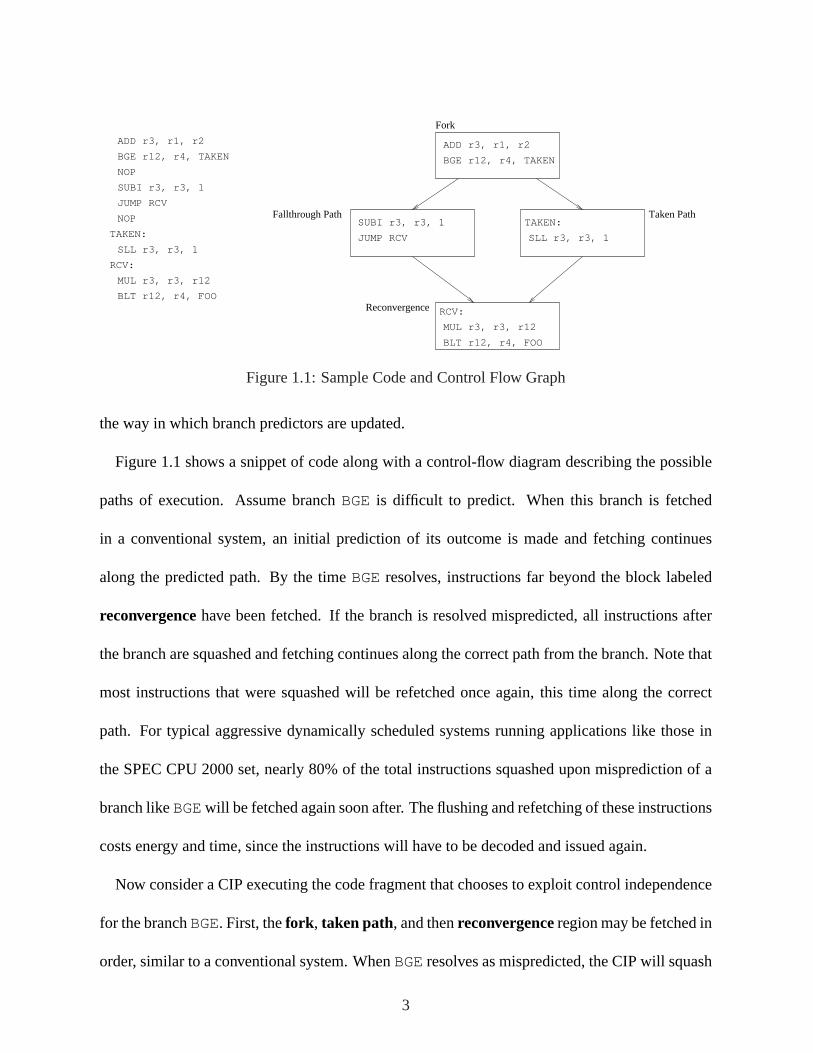
Figure 1.1: Sample Code and Control Flow Graph
the way in which branch predictors are updated.
Figure 1.1 shows a snippet of code along with a control-flow diagram describing the possible
paths of execution. Assume branchBGE is difficult to predict. When this branch is fetched
in a conventional system, an initial prediction of its outcome is made and fetching continues
along the predicted path. By the timeBGEresolves, instructions far beyond the block labeled
reconvergencehave been fetched. If the branch is resolved mispredicted, all instructions after
the branch are squashed and fetching continues along the correct path from the branch. Note that
most instructions that were squashed will be refetched once again, this time along the correct
path. For typical aggressive dynamically scheduled systems running applications like those in
the SPEC CPU 2000 set, nearly 80% of the total instructions squashed upon misprediction of a
branch likeBGEwill be fetched again soon after. The flushing and refetching of these instructions
costs energy and time, since the instructions will have to be decoded and issued again.
Now consider a CIP executing the code fragment that chooses to exploit control independence
for the branchBGE. First, thefork , taken path, and thenreconvergenceregion may be fetched in
order, similar to a conventional system. WhenBGEresolves as mispredicted, the CIP will squash
3

CIP weakened
CIP
ConventionalFork
Fork
Fork
Taken
Taken
Taken
Doomed Instructions Weakened Branch Resolves
Reconv. cont’d
Reconv. cont’d
Reconv.Reconv.
Reconv.
Reconv.
Not T.
Not T.
Not T.
Time
Far
Far
Weakened Branch Fetched
Figure 1.2: Fetch Stream Comparison
only thetaken path region and fetch thefallthrough path retaining all control independent in-
structions in the pipeline while recovering from the branch misprediction. Afterfallthrough path
is completely fetched, fetching will continue where it left off whenBGEresolved mispredicted.
A CIP will speed this execution because fetch bandwidth is not wasted by squashing and
refetching the instructions in the reconvergence region and beyond, as shown in Figure 1.2. The
highlighted regions in the figure indicate the fetching of doomed instructions. Notice that in the
conventional case, thereconvergenceregion is squashed and later refetched. The second diagram
shows what would ideally happen in a CIP. Because there is less time spent fetching doomed
instructions, some subsequent region of codefar is fetched sooner than in the conventional case.
In the third diagram, the impact of weakening is shown. Some branch in thereconvergence
region, which would not be mispredicted in the conventional case, is mispredicted in the CIP.
As a result, the system fetches considerably more doomed instructions. In this case, weakening
has caused control independence exploitation to slow execution down rather than speed it up.
Comparing the diagrams of the conventional system and the weakened CIP, it is evident that
more of the fetch bandwidth is wasted on doomed instructions in the weakened case. It becomes
clear that to exploit control independence as much as possible, there should be some action taken
4

to minimize negative effects caused by branch weakening.
Weakening is caused by two broad reasons. The increase of in-flight instructions and the
prolonged commit times of branches in a CIP cause predictors to be updated differently than they
would in a conventional system. Additionally, if predictors in the conventional system update
earlier than commit time, the additional speculative execution required by a CIP could induce
incorrect predictor updates. This type of weakening involving predictor update times may be
avoided through techniques that selectively update the predictor earlier than the time at which
branches commit. The other broad cause of weakening is caused by incorrect or missing branch
outcomes in the GHR of CIPs. This property either introduces useless outcomes into the outcome
history, callednoise ingestion, or robs the history of important correlation data, calledsignal loss.
The termnoiserefers to a branch outcome that varies in the GHR that isn’t correlated to any
branch which uses it for prediction. Noise ingestion causes branches in a CIP to be associated
with more table entries in the predictor. Each of these extra entries will need to be trained and the
mispredictions due to this cause weakening. Weakening due to noise ingestion can be alleviated
with outcome history update methods that reduce the amount of unnecessary outcomes brought
in to the GHR when exploiting control independence. The termsignalrefers to a branch outcome
in the GHR that is useful for correlation of branches that use it. When branches are weakened due
to signal loss, the more common case is that the weakening cannot be avoided since the correct
outcomes cannot possibly be determined. This type of weakening cannot be reduced. In other
less likely cases the signal is discarded as a side effect of fetching out of order which can be
avoided by careful GHR management.
If weakened branches are classified into the reasons just presented, then the amount of avoid-
5

able weakening may be measured. The goals of this study are as follows. First, to develop
definitions, identify characteristics, and quantify the major types of weakening. This includes a
full analysis of the CIP artifacts that cause each type of weakening. Second, to provide an un-
derstanding of how each type of preventable weakening may be avoided while providing insight
towards how much weakening is inevitable. The final goal is to develop techniques to lessen the
effects that cause weakening using a fundamental approach brought about by achieving the prior
goal.
6

Chapter 2
Background
2.1 Branch Prediction
In early pipelined single-issue processors, branches could resolve one cycle after being fetched.
Instead of leaving a bubble of inactivity in the pipeline, every branch had a subsequentdelay
slot instruction that would be executed independent of the branch’s path. Since correct branch
outcomes were usually available when needed, no branch predictor was necessary. Current gen-
eration superscalar processors fetch many instructions per cycle and contain many more pipeline
stages [Sit93, Sto06, Sto01, TDF+02]. This greatly enlarges the potential bubble, making delay
slots unreasonable and branch prediction vital.
A basic blockis a sequence of code in which execution always starts with its first instruction
and ends with its last instruction with no branching in between. A basic block contains at most
one branch instruction and this instruction must be at the end of the basic block. Abranchis an
instruction that usually1 tests a condition to control the flow of instructions. A branch can either
betaken, denotedT, or not taken, denotedN, and this is referred to as the branch’sdirection. If a
branch is not taken, then the instruction in the program that comes after the branch is fetched. If
taken, then control flow changes to some destination address specified by the branch instruction.
A static branchis an instruction in code that resides in some memory location. Fetching a static
branch creates adynamic branch. A dynamic branch is said to bein-flight from the time it is
fetched to the time it has been committed or squashed. Multiple in-flight dynamic branches
may correspond to a single static branch. Abranch predictoris an architectural component in
1Some instruction set architectures contain branches that are always taken.
7

the processor that tries to determine the direction of a branch in order to increase instruction
throughput. Thebranch target bufferis a component that tries to provide the target of a taken
branch before it is computed later in the pipeline. A dynamic branch is said toresolvein the
cycle that its condition is tested. If the branch is mispredicted, the CPU must perform arecovery
by squashing all instructions after the mispredicted branch and resuming fetch along the correct
path of the branch. At some point after a branch’s resolve time, it updates its predictor entry to
reflect its direction. This occasion is simply referred to as branchupdate. Further detail regarding
the fundamentals of branch prediction and other modern computer architecture concepts can be
found in the Hennessey and Patterson texts [HP03, HP08].
The metrics used to measure the performance of branch predictors are thebranch prediction
ratio and thebranch misprediction rate. The branch prediction ratio is the number of correct
predictions divided by the total number of predictions of some defined execution. The branch
misprediction rate is the number of branch mispredictions divided by a given rate of instructions.
Branch prediction ratios and branch misprediction rates in this study are always measured for
only committed branches. The misprediction rates are measured in mispredictions per 1000
committed instructions, denotedmisp/kI.
There are special prediction techniques forindirect branches, those that branch to a target
specified by a register. The address to which these instructions branch may change throughout
execution. These types of predictors are not considered in this study.
2.1.1 Common Predictors
Simple predictors, such as the that in the ARM810 processor [ARM], implementstatic branch
predictionschemes. In these schemes, prediction is based on the static branch and is used for
8

all dynamic instances of that branch. More modern predictors such as the Pentium 4 use a static
predictor while the system’s more complex predictor is training [Sto01]. The static predictors
in these architectures predict all forward branches (branches whose target is further in code) not
taken while all backwards branches are predicted taken. This is intuitive, since most backwards
branches belong to loops and are expected to be taken most of the time. In an early study by
James E. Smith, the need fordynamic branch predictionwas addressed [Smi81]. Dynamic branch
prediction schemes predict branches based on program run-time characteristics. For example, a
branch may be predicted as its last resolved outcome in a program. The Smith study shows that
on average about 4% improvement in branch prediction accuracy for a small set of benchmarks
can be attained using this very simple method over a static scheme where branches are predicted
based on their operation codes. More advanced dynamic predictors discussed in the remainder of
this section can drastically improve basic static schemes, increasing the branch prediction ratio
by 40% in some cases.
The bimodal predictor [Smi81] is a popular and relatively simple dynamic branch predictor.
It is a per-address branch predictor, meaning it indexes abranch history table(BHT) using the
address of the branch it is predicting. Each BHT entry consists of a 2-bit saturating up-down
counter. Note that though some predictors may implement some other finite automaton for their
table entries, all predictors in this study use an up-down counter. The most significant bit of the
counter indicates the prediction of the branch. In this study, it is assumed that the branch will
be predicted not taken if this bit is 0 while the branch is predicted taken if this bit is 1. Upon
predictor update, the counter will be incremented or decremented based on the branch’s correctly
resolved direction. A not-taken outcome will decrement the entry while a taken outcome will
9

increment it.
More advanced dynamic branch prediction techniques use two levels of branch history. Tse-
Yu Yeh and Yale N. Patt studied and compared some variations of two-level predictors [YP92].
These predictors were both per-address andcorrelating, meaning that some type of outcome
history data is used to make each prediction. The GAg predictor described in the study is an
example of a correlating predictor. A special register, named theglobal history registeror GHR,
keeps a record of the lastk outcomes of branches that executed. At predict time, the GHR is used
to index apattern history table, or PHT, of saturating counters and a prediction is made using the
counter’s value. Once the branch’s outcome is known, this entry is updated appropriately. This
predictor is named GAg to stand for Global Address, global PHT.
The best performing predictor in the study is the PAg predictor (per-address, global PHT). A
first table is indexed by a branch’s address and contains thelocal historyfor the branch. This is
the sequence of outcomes for the lastk instances of the static branch. The local history will then
index a global PHT that contains a saturating counter used for prediction. The study showed on
a whole that various dynamic two-level branch predictors yield a 97% accuracy on average for
various SPEC92 CPU benchmarks.
In a study by Scott McFarling in 1993, the GShare predictor is introduced [McF93]. GShare
is a two-level predictor whose global and per-address information are shared in the first level by
XORing the PC and global history. This value indexes a PHT of saturating counters that yields the
prediction. This is a popular and well performing predictor, averaging near 97% accuracy under
selected benchmarks with a 32kiB table. An important technique introduced by McFarling in this
study is the combining of branch predictors to form ahybrid predictor. This type of predictor is
10

built to select the better prediction option of any two predictors. It uses achoosertable, which is
a per address table of two-bit saturating counters. On a branch prediction, the chooser will select
either of the two predictors. On update, if one and only one of the predictors mispredicted, the
chooser entry will be updated towards choosing the one that is correct. A 32kB bimodal/GShare
Hybrid predictor outperforms a 32kB GShare predictor in every benchmark selected for the study.
There are many other predictors that correlate on some form of global history [EM98, YP93].
Some predictors, such as the perceptron predictor [JL01], are much more advanced than ones
described here. Though these predictors are valuable, their complexity makes them less practical
for study. Due to its ease of understanding, GShare is the only correlating predictor (or predictor
component) that will be used in this study.
Numerous current-generation processors use correlating predictors to improve performance.
One example is Intel’s Core processor which was designed with a relatively more complex
predictor than others implemented at the time [Sto06]. The branch predictor has a type of bi-
modal/global hybrid component similar to the hybrid predictor used in this study. The predictor
also has a specialloop detectorcomponent that predicts when loops will terminate. The archi-
tecture also implements an indirect branch predictor.
Another example of a modern processor that uses a correlating predictor is the IBM POWER4
architecture [TDF+02]. It also has a similar type of hybrid predictor. The per-branch component,
called alocal predictor, is a 16k-entry BHT consisting of 1-bit entries. The correlating predictor
component, called aglobal predictor, uses an 11-bit vector, much like a GHR, called aglobal
history vector. This register isXORed with the PC to index aglobal history tableof 1-bit entries.
The chooser component, called thesector table, is also a table of 1-bit entries but, unlike GShare,
11

it is indexed in the same manner as the global history table.
2.1.2 Correct and Timely History Update
A wrong path history updateoccurs when a doomed branch updates the branch predictor. The ef-
fects of wrong path history updates have been presented by Jourdan et al. [JSHP97]. In the study,
several predictors, GShare being one of them, updating outcome history at predict time are com-
pared to their counterparts that update non-speculatively at commit time. Several mechanisms
are covered that enable speculatively updating history at branch predict time while assuring that
the history is correct. It is shown that performance drops by 30% on average if speculative global
histories are not repaired across the proposed techniques. The predictor component that causes
most of this degradation is the GHR. This suggests that some checkpointing mechanism that re-
pairs the GHR on a misprediction is vital to the predictor. Because branches may resolve out
of order, a PHT entry may be erroneously updated if predictors are set to update at resolve time
(for example, when a doomed branch resolves). The study reveals that this speculative updating
of the PHT without repair has almost no effect on performance. However, a BHT may be more
vulnerable to incorrect updates since instances of the same branch tend to appear closer together
in execution compared to instances of the branch reached by same path.
Branch predictors that have long prediction latencies either cause the CPU clock to have a
lower frequency or require a pipelined implementation of the predictor. Pipelined predictor im-
plementations leave bubbles in the instruction pipeline, decreasing the fetch rate. Daniel A.
Jimenez et al. establish that it is not enough for a predictor to attain a higher accuracy, it must
also provide a timely prediction [JKL00]. One technique offered in the study to improve the
performance of systems with more complex predictors isoverriding: Using a smaller and faster
12
predictor to make an initial 1-cycle prediction while waiting for more accurate prediction from
a larger more complex predictor. A study by Gabriel H. Loh explores, in addition to prediction
latencies, that predictor update latencies are also a significant factor of performance degradation
– especially on deeply pipelined (40-stage) systems [Loh06]. The study shows that when using
an overriding predictor the more complex component, in this case perceptron, can be used to
provide a quick (though perhaps incorrect) update to the smaller 1-cycle component, GShare,
to attain about 5% speedup in IPC for selected SPEC CPU benchmarks on a 40-stage pipelined
system. This technique is calledhierarchical update. It is claimed that update latency of highly
accurate predictors are only affected by update latency in the initial training phase of the predic-
tor, while smaller predictors are much more vulnerable due to their size.
2.2 Paths
For a correlating predictor, entries in the predictor’s PHT correspond to paths by which the pre-
dicted branch was reached. In this study, the termpath is the PHT index used when predicting a
dynamic instance of a branch. The branch is said to bereached bythe path. The GShare predictor
used in this study constructs its path byXORing ak-outcome GHR tok bits of the branch PC.
Define thetrue pathas the path reached by a non-doomed instruction in a conventional system
that maintains a correct GHR and computes the path as defined by the predictor. Apure path
of a branch is a sequence of the lastk correct global outcomes in program order (equivalently,
the contents of a k-bit GHR on a conventional system). Any path observed by a non-doomed
instruction is referred to as anobserved path. It will be shown further in the study that observed
paths may not always be true paths in a CIP.
The path filtered local historyof a static branch for some given path is the local history for
13

Table 2.1: Branch Behavior DefinitionsName Definition Example
Mono- M0(B) <= M1(B)Monostable M0(B) = 0 TTTTTTTTTTTTTMonoloop M2(B) = 2M1(B) TTTNTTTTTNTTTMono-other All other mono-
Bi- M1(B) < M0(B)Bistable M1(B) < M2(B) NNNNTTNTNTTTTBibiased M2(B) = 2M1(B) TTTTTTNNNNNNNOther All other behavior
that branch which only includes outcomes of the branch reached by that path. Path filtered local
history is used to study branch outcomes relevant to correlating predictors.
Because many branches may share PHT or BHT entries, branch predictors are subject tocol-
lisions which hurt branch prediction accuracy. A collision occurs when a branch uses some
predictor entry it had previously updated but had since been updated by some other branch.
If every path of every branch had its own PHT entry, the pattern index computed using a simple
hashing would have to bek + b bits long, where2b is the maximum number of static branch
instructions allowed. For some reasonablek, the size of this PHT would be wildly impractical.
This is the reasonoutcome history hashingis used to generate a reasonably sized path. Call an
optimal outcome history hashone that yields the highest branch prediction accuracy for a given
PHT size. The GHRXORPC hash of the GShare predictor is a sound approach since it enables
the path to be influenced by both the static branch and the global history. However, there may
be better outcome history hashing allowing for accuracies closer to the optimal. Understanding
branch behaviors may allow for better hashing techniques, but analyzing it out of the context of
weakening is beyond the scope of this study.
14

2.3 Branch Behavior
There are several behaviors exhibited commonly by branches. Classification of branches by
their behavior helps bring about understanding as to how branches are weakened. DefineB as
the full outcome sequence of some static branch. LetM0(B) denote the number of timesB is
mispredicted when using aperfect static predictor. A perfect static predictor has prior knowledge
of the most frequent direction inB and always predicts the branch in that direction. LetM1(B)
andM2(B) denote the number of times a dynamic bimodal predictor mispredicts the branch with
a 1-bit saturating counter and 2-bit saturating counter, respectively.
The definitions of several branch behaviors are given in Table 2.1. Branches that favor a static
prediction are named with the prefixmono-while those that prefer dynamic prediction are named
with bi-. Typically in literature, the termbiasedis used to describe what is referred to here as
monostable behavior whenB contains all taken or all not-taken outcomes. The monoloop behav-
ior is typically referred to as just aloopbehavior, whenB contains all similar outcomes separated
by single opposing outcomes. Monostable and monoloop branches are predicted accurately with
a bimodal predictor. Monoloop branches are predicted best with a 2-bit saturating counter, since
using a 1-bit saturating counter causes an extra misprediction of the branch after every loop exit.
This may be in part the reason why most branch predictors employ 2-bit counters as opposed to
other sizes. Two mono- branches are calledunanimousif their favored outcomes are in the same
direction. The branches are said to bedissonantif their outcomes are in opposing directions.
Bistable and bibiased branches exhibit longrunsof the same outcome, where a run is a subse-
quence of similar outcomes for a branch. A branch classified as bibiased has only large runs in
its outcome history, therefore a predictor with a 1-bit saturating counter will yield half the mis-
15

predictions of a predictor with a 2-bit counter. The bistable class allows for a little more leniency.
Branches can be classified this way if they are more accurately predicted with a predictor using
a 1-bit saturating counter than one using a 2-bit saturating counter. Recall that for both of these
behaviors, a 1-bit saturating counter outperforms a perfect static predictor.
Though the definitions above specifically refer to the behavior of a branch’s local history, they
apply to path filtered local histories as well. The implications of each static branch’s local history
behavior on a per-address predictor such as bimodal carry on to the branch’s path filtered local
histories on a correlating predictor. For the remainder of the section, branch local histories will
be used to describe behaviors, but path filtered local histories apply as well.
The plot in Figure 2.1 shows the measurement of branch behaviors as defined above for
branches and 16-bit paths. Paths are constructed byXORing the 16 bits of the branch’s PC with
16 bits of the global history, similarly to the way GShare constructs paths. Results are shown as
percentages of dynamic branches. The benchmarks are those selected for this study and will be
presented in detail later in Section 5.1 along with RSIML, the simulator used to collect results.
These results are taken directly from RSIML output, which includes the classification in its dis-
tribution. Results are gathered via functional simulation. The way in which the classification is
performed will now be discussed briefly.
The module of RSIML that classifies branches and path filtered local histories assigns a pre-
defined class to each branch or path by using the branch prediction accuracies of a set ofn i-bit
saturating counter predictors. The counter predictors for each branch or path are incremented
if taken and decremented if not taken. The most significant bit of the counter is used to make
a prediction. If the first outcome of the branch or path is T, the counter is set to its maximum
16

0
20
40
60
80
100
% o
f Tot
al D
ynam
ic B
ranc
hes
Bra
nch
20
40
60
80
100
gzip swim vpr.p vpr.r gcc art mcf craftyfacerec
parserperl gap bzip2
twolfmesa
% o
f Tot
al D
ynam
ic B
ranc
hes
16-b
it P
ath
Benchmark
BibiasedBistable
MonostableMonoloop
Mono-otherOther
Figure 2.1: Classification of Branches and 16-bit Paths (petdis.134, functional simulation)
17

value. If N, it is set to zero. Predictors of size 1 to 6 bits are used and in addition the total
number of taken outcomes is tallied. LetMi(B) denote the number of mispredictions of ani-bit
counter predictor.M0(B) is a special case that denotes the number of the less common outcome
in the local history of a branch (this is the number of mispredictions yielded by a perfect static
predictor). LetMm(B) be the minimum numberMi(B) for all i from 0 to n. Branches are then
classified in the following order.
Monostableif M0(B) = 0; else,
Monoloopif M0(B)−M1(B)/2 < 2; else,
Mono-Otherif M0(B) <= Mm(B); else,
Bistableif M2(B) > M1(B); else,
Bibiasedif Mm(B) > 1.01M0(B); else,
Other
Referring back to Figure 2.1, note that many of the benchmarks have significant amounts
of bistable and bibiased branch and path behaviors. Branches of these types certainly prefer a
speedy predictor update and suffer more training mispredictions, as will be explained in more
detail further in the study when discussing weakening.
2.4 Branch Overlap and Update Lag
Branchoverlapbecomes important when studying weakening dealing with predictor update. A
branch is said to overlap if one dynamic instance of the branch is predicted before a prior non-
doomed instance of the same branch updates its predictor entry. This behavior is usually exhibited
in tight loops when the system is executing many instances of a small group of static instructions.
A path is said to overlap if one instance of the path is predicted before a prior non-doomed
instance of the same path updates its predictor entry. This is referred to aspath overlap.
18

F D E R C
F D E R C
Update Lag
F: FetchD:DecodeE:ResolveR:ReadyC:Commit
Predict Time Update Time
0x1ccc8 bne,a
...
0x1ccc8 bne,a
...
0x1ccc8 bne,aF D E R C
Figure 2.2: Example of overlap taken from the bzip2 benchmark
Call the time from when a dynamic branch is predicted to the time the predictor is updated the
update lag. Update lag can be measured in many ways. Call thecycle update lagthe number
of cycles from predict to update of a branch. Call theinstruction update lagthe number of
instructions fetched from predict to update of a branch. Thebranch update lagis the number of
branches fetched from predict to update of a branch.
There are cases in which conventional systems are sensitive to update lag. An overlapping
branch is shown in the pipeline execution diagram of Figure 2.2 with the update lag for the first
instance marked. Assume this branch to be a simple if-then-else statement within some loop
body. Other instructions and all squashed instances of the branch have been removed for clarity.
Assume the branch to be bistable. The first instance shown represents the beginning of a run.
When this instance resolves, it squashes all subsequent instructions and fetches along the correct
path (The instance does not commit right after resolving due to out-of-order execution). Notice
that all other instances shown in the figure are fetched along the correct path, but do not see the
update of the first instance. All the instances will mispredict. If the update lag were decreased
by setting the predictor to update at resolve time, each instance will see all prior updates. The
reduction of update lag causes the third instance to be predicted correctly. Situations like these
19

do not occur too often in conventional systems because branches usually commit soon after they
resolve. It will be shown further in the study that lag and overlap are more relevant in a CIP.
Intuitively, branch overlap is expected to happen more frequently than path overlap. This is
because when two instances of a static branch overlap, their paths may be different. Even so,
there may still be plenty of path overlap in execution. This will be revisited and elaborated with
data further in the study.
20

Chapter 3
Control Independence
A non-doomed dynamic instruction is control independent (CI) of a candidate dynamic branch if
it is fetched regardless of the direction of the candidate [LW92]. Instructions are control depen-
dent (CD) if they are fetched on only one direction of the candidate.
Refer back to Figure 1.1. Recall that branchBGEis a difficult branch to predict, so the CIP
may protect it, exploiting control independence so that fewer instructions are squashed when
it is mispredicted. BranchBLT is the first branch control independent ofBGE– meaning that
it can be reached on all paths fromBGE. The first instruction in the basic block belonging to
BLT is called thereconvergence pointof BGE. A conventional processor would squash, along
with any other wrong-path instructions, the reconvergence point instruction and all subsequent
instructions on misprediction of the protected branch. This is wasteful because these instructions
are soon refetched after the squash. In the selected benchmarks used in this study, the number of
cycles it takes a branch to resolve vary from 30 to 140, with the average being 40. Since there are
8 instructions fetched per cycle, this means that on average there are potentially 320 instructions
that may be squashed upon a misprediction. Since many branches have reconvergence points
nearby (usually less than 16 instructions [CTW04]) there is high potential benefit for CIPs.
There are several implementation issues of control independence that can ruin its potential for
benefit. In the introductory example, the later squashedtaken path block of code changed the
value of registerr3 before the squash. The CIP must re-execute the post-reconvergent instruc-
tions with the correct value ofr3 (the value it was set to before the branch). This is just one
21

example of implementation issues that CIPs must address to maintain program correctness while
fetching out of order. Realistic mechanisms implemented to maintain program correctness are
required for any CIP implementation.
3.1 Implementation Issues
3.1.1 CD- or CI-First
There are two fetch techniques a CIP may implement.CD-First is a technique where a CIP
fetches just as a conventional system would until a protected branch resolves. If it resolves cor-
rect, execution continues similarly to the conventional case. If it resolves mispredicted, only CD
instructions are squashed. The correct path instructions will be fetched and executed while any
post-reconvergent instructions are still in flight. Once the entire CD region is fetched, fetching
continues at the point where it was at the moment just before the protected branch resolved. The
post-reconvergent instructions may need to be re-executed in order to maintain program correct-
ness. The example given in the introduction reflects this technique.
CIPs that employ theCI-First technique begin fetching post-reconvergent instructions immedi-
ately after fetching the protected branch. Once the branch resolves, the correct path CD region is
fetched and executed. Similarly to the previous technique, after the CD instructions are fetched,
the post-reconvergent instructions may need to be re-executed to maintain program correctness.
Notice that this technique eliminates the need to initially predict a direction for protected branches
and so there is no need to squash.
3.1.2 Register Remapping and Speculative Execution
Dynamically scheduled processors map an instruction’s destination register to a freshly allocated
physical register and read mappings for the instruction’s source registers. This mapping enables
22

instructions that write the same architected register to execute out of order. Since they write
different physical registers, no data is lost.
The mappings of instructions past the reconvergence point may depend on the path taken
through the control dependent region (CDR). In execution, it is common to have register de-
pendencies between the CDR and post-reconvergent instructions. The CIP may not be aware of
these dependencies until a protected branch resolves. Once the correct CDR is fetched, the regis-
ter mapping becomes defunct and must be repaired to maintain program correctness. Therefore,
any CIP must take the steps needed to correct register mappings when performing a protected
recovery.
Some CIP implementations correct the mapping usinginjected instructions[CV01, AZRRA07].
After executing the CD instructions and before continuing execution of post-reconvergent instruc-
tions, specialMOVinstructions will correct the mapping. The example at the beginning of this
section refers to the registerr3 of Figure 1.1. Assume the code in the figure is running on a
CIP and that the “Taken Path” block was just squashed while the post-reconvergent code is still
in flight. At this point, theMULinstruction has operated on the incorrect value ofr3 . To repair
this, the CIP will inject a special instruction into the pipeline that will write the value ofr3 to the
value that it was before the incorrect CDR changed it. This way, post-reconvergent instructions
may re-execute using the correct value.
Instructions that depend on registers that may be incorrect must be executed speculatively until
any downstream CD region resolves. Once the register mapping is correct, dependent instructions
are re-executed. Furthermore, instructions that consume data from these instructions must also be
re-executed, and so on. When a branch is re-executed,vacillationmay occur. A branch vacillates
23

when it changes its resolved direction due to re-execution. It is possible for a single instance of a
branch to vacillate more than once. Vacillation is a very important overhead of CIPs. Its impact
to combat certain types of weakening will be elaborated further in the study.
3.1.3 Finding the Reconvergence Point
Reconvergence point detection is crucial in a CIP because it partitions the control dependent and
control independent instructions for a protected branch. There are several techniques that find or
predict it with reasonable accuracy both statically [SBV95] and dynamically [AZRRA07, CV01].
In one dynamic implementation [Kop08], each of the instructions on separate paths flowing from
the protected branch are tagged with a different color for each path. The reconvergence point
will be the first instruction tagged with both colors. Since the CD region is found dynamically
in this way, the candidate branch must execute at least once on both paths. The mechanism
also considers return instructions. If both paths from a protected branch lead to a return, the
reconvergence point would then be the target of the return.
In a separate implementation [CV01], the reconvergence point can be found dynamically by
searching forif then else and similar control flow structures. This is done by checking
if the first instruction after a branch (not including delay slot instructions) is the target of a re-
cent branch. Higher level constructs likeif then else andcase have easily identifiable
reconvergence points. For example, theif clause andelse clause are control dependent while
anything after theif then else construct is control independent.
An advanced and highly accurate dynamic reconvergence prediction scheme was introduced
in a study by Collins et al. [CTW04]. Branches are classified into several categories that are
defined using analysis of program control flow graphs. For example, the most common case is
24

for a branch’s reconvergence point to occur later in code (meaning the reconvergence point’s PC
is greater than the branch’s PC), while no instruction past the reconvergence point ever executes
in the CDR for some level of the function call stack. This case is handled by the reconvergence
predictor that skipper utilizes; however, skipper assumes certain compiled instruction layouts and
only handles this single case. Another case handled in the study, though not as common, occurs
when there are multiple return instructions in the CDR. An aggressive hardware implementation
that categorizes branches into one of four behaviors, including those just presented, predicts
reconvergence points with 99.9% accuracy for most of the studied benchmarks. A more feasible
implementation of the predictor achieves over 95% prediction accuracy.
3.1.4 Selective Squashing
In conventional systems, instructions are kept in there-order buffer(or similar) from the time they
are initially fetched until they are committed or squashed. The re-order buffer (ROB) is generally
a FIFO that serves many critical functions. It assures that instructions commit in order (though
they may execute out of order) and provides a means for recovery upon branch mispredictions
or exceptions. Control independence exploitation poses a problem for conventional ROBs due to
out-of-order fetching. The ROB may need to be redesigned to leave a gap for any later incoming
CD instructions when a protected branch is fetched.
In many implementations, the size of the gap can be guessed similarly to the way reconver-
gence points are predicted. Accuracy in gap size detection is crucial since all instructions after the
protected branch will have to be flushed if the gap size is inadequate. Furthermore, overshooting
the gap uses unneeded space in the instruction window which may eventually cause the fetch unit
to stall.
25
3.1.5 Targeting Branches That Are Difficult to Predict
A CIP implementation may turn protection for branches on (and in some cases, off) during exe-
cution [RSI, AZRRA07, HR07, CV01] while another may protect every instance of certain static
branches [CFS99, SBV95]. In the former case, referred to as adynamic CIP, some method like
confidence estimation(described in the next paragraph) is used to dynamically determine candi-
dates for branch protection. In the latter case, called astatic CIP, some type of instruction set
architecture support is necessary to convey information regarding candidates for protection to the
system. This information may be generated by the compiler by way of techniques such as static
code heuristics or training input sets.
Confidence estimation is a technique used to detect if a branch is likely to be mispredicted.
A study by Erik Jacobsen et al. presents several different one- and two-level confidence esti-
mators [JRS96]. In one of the more successful one-level implementations, a table called the
Correct/Incorrect Register Table, or CIR Table, is indexed similarly to a PHT to yield whether
or not a branch is likely to mispredict. Each entry of the CIR Table is 4-bits, and each of these
entries are initialized to all ones. A branch is considered likely to be predicted correctly if its CIR
Table entry is 15. If a branch is predicted correctly, this entry is incremented (though it saturates
at 15). If the branch is mispredicted, the entry is reset to 0. This relatively simple technique
proves effective, isolating nearly 90% of mispredictions for selected benchmarks.
For a detailed comparative analysis on the confidence estimation method described above as
well as several other techniques, consult the study by Grunwald et al. [GKMP98].
26

3.1.6 Areas of Low Potential for Benefit
Not every application benefits from control independence. There will be little benefit in protect-
ing branches with a very distant reconvergence point. The hindrance is due mainly to the amount
of instructions that will be squashed on a protected recovery. A CIP may also not show much
benefit if the CDR contains dependencies along the critical path. Though the post-reconvergent
consumers will not be squashed, they will have to wait for the protected branch to resolve any-
way. This generally increases the number of in-flight instructions and could cause the ROB to fill,
stalling the fetch unit. Additionally, codes high in weakening and vacillation tend not to benefit
and in some rare cases may exhibit performance degradation. Nevertheless, the majority of ap-
plications in the benchmark set selected for this study enjoy the benefits of control independence.
3.2 Snipper
Snipper is the CIP selected to be used for this study [Kop08]. It is named so because the term
snip is used to refer to a control dependent region and its context. It attains speedup competitive
with other researched CIPs, but does so in a unique way. As other CIPs choose where to exploit
control independence based solely on branch confidence estimation [CV01, HR07] or detection
of a reconvergence point [AZRRA07], snipper additionally uses a performance estimator to judge
where exploiting control independence would be beneficial. This is helpful, as there are common
situations where protecting branches may not result in speedup or may even hinder execution.
Protecting a branch is not beneficial when the branch isexecute-or commit-critical. As defined
in a study by Fields et al., a branch is execute-critical when there is a critical path data dependency
in its CD region [FRB01]. Exploiting control independence in this case does not help since it is
the branch’s resolve time that is the bottleneck. In fact, mainly due to vacillation, covering
27
execute-critical branches can in some cases lengthen the resolve time of other branches, causing
slowdown. A branch is commit-critical when it is the next instruction to commit and is preventing
other instructions from being fetched because the ROB is full. In other words, the CPU cannot
accommodate more instructions until the branch commits. If the system’s instruction window
size were larger, the branch would no longer be commit-critical.
Snipper protects branches only when itsreduction estimatordetects possibility for speedup.
The reduction estimator used for this study, namedfetch-cycles, evaluates whether or not a branch
is execute- or commit-critical. It does so by way of bookkeeping certain characteristics of snips.
For example, one of the values recorded is number of cycles spent fetching CI instructions from
when a branch is mispredicted until it is resolved. The estimator also checks for a full ROB as
well as whether or not the branch is near the head of the ROB. For more details on reduction
estimators, a thorough study has been conducted by Koppelman [Kop08]. In the study it is
shown that using such reduction estimators avoids slowdown in areas of execution where control
independence cannot be effectively exploited.
At a lower level, snipper is a relatively simple CD-First CIP. Instructions are re-executed with-
out changing their original register mapping. It does this by injecting specialMOV[SI94] in-
structions calledpmoves[KG99] that correct values in the mapped physical registers of control
independent instructions. More than one pmove of any architectural register may have to be in-
jected, depending on the number of times the register was written in the doomed CDR. Using
the injected instructions allow post-reconvergent consumers to remain in the scheduler without
having to be renamed, though they will need to re-execute.
Information for snips is kept in asnip information table. This table includes data such as the
28

candidate branch’s PC, the reconvergence point, and a score used to determine whether or not
exploiting CI for the candidate branch is detected as worthwhile. The reconvergence point is
found using the coloring method described in Section 3.1.3. The colored tags are referred to as
cookiesin the snipper nomenclature. Information about cookie locations is kept in thecookie
table.
Snipper turns protection of a branch on and off depending on whether or not potential benefit
is detected. This is useful when the path to a protected branch changes at different points in the
program; for instance, if the branch is in a subroutine called from many different parts of program
execution. The reason for dynamic protection of this caliber is that, as has been said, sometimes
exploiting control independence does not help. Snipper can also run as a static CIP so that each
static branch is either always or never protected. More information regarding this is provided in
Section 5.2.
The default predictor used by snipper is the YAGS predictor developed by Eden and Mudge
[EM98]. This predictor correlates branches on global outcome history via the GHR. YAGS is
not used in this study since the way in which it makes predictions is more complex than GShare.
Nevertheless, the hybrid predictor used here performs just as well or better for most benchmarks
and is more widely studied.
Snipper’s approach to history update is to always insert CDR data into the GHR and use it for
prediction and update, regardless of whether or not it is correct. This method is used because it
yields better results than not including CDR data into the global history.
Figure 3.1 shows the speedup of a system exploiting control independence using snipper. Re-
sults are shown for the system branch predictor as bimodal, GShare, and hybrid.
29

0.8
0.9
1
1.1
1.2
1.3
1.4
1.5
gzip swim vpr.p vpr.r gcc art mcf craftyfacerec
parserperl gap bzip2
twolfmesa
Spe
edup
Benchmark
bimodalgsharehybrid
Figure 3.1: Snipper Speedup (petdis.69, pad-cdr)
30

Snipper is described here only to the point of detail necessary to discuss branch weakening.
For more details, consult the study by Koppelman [Kop08].
31
Chapter 4
Prior Work
4.1 Limit Studies
Several studies have qualified that returns of exploiting control independence are worthwhile. A
study by Lam and Wilson shows the amount of parallelism that can be obtained with control
independence exploitation on an abstract system [LW92]. The system models used in the study
enforce true data dependencies and control flow while ignoring memory disambiguation, non-
true data dependencies, and resource limitations. There are an unlimited number of functional
units and instructions are fetched and committed in one cycle. The system model of interest for
the purposes of control independence as studied here is the SP-CD-MF model. It is an ideal
control independence system with multiple flows of control, meaning branches may execute out
of order and only CD branches will be squashed on a misprediction. This model can be compared
to another model in the study named SP. SP is simply a system modeled with only a branch
predictor. Each system uses a perfect static predictor for branch prediction. Results show that
the SP-CD-MF system can attain 23 times the parallelism of the SP system on average across the
selected non-numeric benchmarks. When limiting control flow by forcing branches to execute in
program order (this is the SP-CD model), the speedup over the SP system drops to about 15. The
study concludes that parallelism is highly limited by control flow in certain programs and though
branch prediction is vital in extracting reasonable amounts of parallelism from them, control
independence significantly helps achieve large amounts of ILP.
Rotenberg et al. similarly compare a set of ideal machine models to evaluate several aspects of
32

control independence [RJS99]. The major difference from the Lam and Wilson study is that the
models respect the need for register remapping and resources used by doomed CD instructions.
As opposed to gathering results from a trace, a pipelined 16-way system with a GShare predictor
is simulated. The model ignores the handling of memory disambiguation, output dependencies,
and anti-dependencies. In addition to wasting fetch bandwidth, doomed CD instructions waste
other resources by remaining in the instruction window until they are squashed. Data dependen-
cies between doomed CDR instructions and post-reconvergent instructions are repaired in one
cycle. It is reported that a model CIP with a 512-instruction window can cut down execution
time 17% on average for the selected benchmark set.
4.2 Branch Classification and Prediction Techniques
Later in this study, weakened branches will be classified by the reason they are weakened. Addi-
tionally, predictor techniques will be offered to alleviate the preventable weakening by modifying
paths and predictor update times. There has been a significant amount of prior works that iden-
tify ways in which path modification can improve prediction accuracy. Significantly less has
been published in classification of branch mispredictions. The studies presented in this section
contribute to the techniques used here to classify and reduce weakening.
An early study by Po-Yung Chang et al. classified branches by the rate at which each static
branch is taken [yCHyYP94]. When branches are classified in this way, certain predictors can be
chosen to predict certain classes of branches. For example, if a branch is classified to be mostly
taken, a static predictor can often perform just as well or better than a correlating predictor in
predicting the branch. The study introduced several hybrid schemes that performed as well or
better than other branch predictors in literature at the time. In a more recent study by Michael
33

Haungs et al., branches are classified by the rate at which they change direction [HSF00]. These
studies use branch classification to build better predictors. In this thesis, however, classification
is used to gain an understanding of why certain mispredictions are caused. There are no efforts
taken to extract performance directly from the classification.
In a study by Kevin Skadron et al., a broad range of predictors are used to develop a taxonomy
of mispredictions [SMC00] to help understand why certain branches are mispredicted. The se-
lected predictors for the taxonomy are chosen carefully based on the information used to make
a prediction. A dynamic branch is predicted through a sequence of chosen predictors. The first
predictor that correctly predicts the branch instance determines the reason for which previous
predictors in the sequence mispredicted it. For example, in the sequence of tests a branch may be
mispredicted by a correlating predictor. The next predictor in the sequence could be a bimodal
predictor. If the bimodal predictor yields a correct prediction, then it can be assumed that the
correlating predictor’s misprediction is due to training a new path. In the study, a new predictor
scheme namedalloyed predictionis developed to fill a hole in the taxonomy by categorizing mis-
predictions due to unavailability of both local and global history. Such study of branch predictor
behavior is of great importance to understanding the causes of weakening.
Paths may be manipulated via code transformations to allow for better prediction accuracy.
In a study by Cliff Young and Michael D. Smith [YS99], a code generation technique used to
obtain better prediction accuracy for correlated branches is explored. Ahistory treeis built from
a program’spath profilethat contains all paths leading to a particular branch. A path profile
is a type of lightweight program trace. Through a technique calledpruning, the history tree is
transformed so that the minimum amount of history to exploit correlation is revealed. Code is
34

transformed using the pruned trees to allow bi- branches to be duplicated so that each copy of
the branch is a mono- branch. The proposed code transforms could improve execution time by as
much as 4% for selected SPEC CPU 1992 and 1995 benchmarks, though the technique slowed
go and ijpeg down by 1-2% due to additional instruction cache misses.
Paths may also be manipulated dynamically to reduce mispredictions. Multi-threaded execu-
tion has the potential to weaken branches because, like in CIPs, branch outcome history is not
available in contiguous program order. In a study by Jayanth Gummaraju and Manoj Franklin, the
effects of single-program (instructions commit in order) multi-threading on branch predictors are
explored [GF00]. It is established in the study that multi-threaded processors’ branch prediction
accuracy is negatively impacted due to several reasons. The study names the reasons insufficient,
discontinuous, outdated, scrambled, or inaccurate history. These different reasons can cause up
to five times more mispredictions for a predictor like GShare on select SPEC CPU 1992 and 1995
benchmarks. It is shown that predictors that use global history are affected much more than pre-
dictors like PAg that use local history, mainly because local predictors are less prone to outdated
information. Anextrapolation/correlation hybridpredictor is developed to address outdated and
scrambled histories. The predictor has two components. The first component uses in-order specu-
lative outcome data to make predictions of branches. This is helpful since update lag is relatively
high for single-program multi-threaded execution. The second component, the correlation-based
predictor, chooses one of several extrapolation predictors based on a thread-level prediction. The
predictor reduces mispredictions by around 3% for most benchmarks.
In another study on path manipulation for multi-threaded processors, Bumyong Choi et al.
built upon Gummaraju and Franklin’s study by focusing on branch prediction for branches in
35

short threads [CPT08]. Since small threads don’t contain enough history for correlating predic-
tors to function effectively, setting the GHR to a thread’s initial PC upon spawning reduced the
misprediction rate by around 29% per thread for a system with a GShare predictor running se-
lect SPEC 2000 benchmarks. This technique allows branches in short threads to correlate to the
thread itself, allowing for less overall training. Leo Porter and Dean M. Tullsen generalized this
technique for a conventional system [PT09]. In the study, it is found that setting the GHR to the
value of the PC in certain situations – namely when leaving a loop – can reduce the misprediction
rate by 12% per kilo-instruction for 32Kb predictors. A small 8Kb or 16Kb GShare predictor
using this technique can perform as good as one twice its size.
4.3 Early Control Independence Processors
4.3.1 Multiscalar
The Multiscalar processor is a multiprocessor which exploits ILP by using a compiler to split a
program into many tasks, each of which is dynamically assigned to one of many processing units
[SBV95]. Each processing unit sequentially executes instructions within its task, and the tasks
themselves are loosely sequentially executed. Register mappings are kept correct through the
use of compiler inserted masks that forward producer registers between processing elements to
future tasks. This serves the same function as the injected instructions mentioned earlier. A task
predictor speculatively assigns tasks to processing units. On a task misprediction, the offending
task and all following tasks are squashed. However, a mispredicted branch within a task whose
control does not leave the task will only cause its own task to be squashed. Because of this,
the compiler’s job of constructing tasks becomes very important. Multiscalar processors exploit
enough control independence to enjoy 2-3 speedup in many chosen benchmarks. Evaluating the
36

weakening caused by using a multiscalar approach is difficult since the multiscalar compiler-
generated code is significantly different from code compiled for a conventional processor with
respect to control transfer.
4.3.2 Dynamic Control Independence
In a study by Yuan Chou et al., a second ROB called theDynamic Control Independence, or DCI,
buffer is used to avoid refetching and renaming control independent instructions upon mispre-
diction of a branch [CFS99]. The study explores both a CI First and CD-First implementation.
It enables control independent instructions that have no CD data dependencies to be copied into
the ROB from the DCI on protected recovery without needing re-execution, though branches are
always re-executed. The implementation uses a GShare predictor that is stated to have “realis-
tic” update, but no further information is given about how history is inserted into the GHR. The
DCI study presents that in an 8-way superscalar processor with a 240-entry ROB can improve
performance by about 15% among selected SPEC CPU 95 benchmarks [DR95]. Although in
nearly every case the CI-First implementation outperforms the CD-First, the authors of the study
claim that the latter appears to be more effective than the former since an unrealistic confidence
estimator was used.
4.3.3 Skipper
The Skipper implementation by Cher and Vijaykumar is a CI-First CIP [CV01]. Skipper pro-
tects only low-confidence branches using a confidence estimator that dynamically tracks branch
performance [JRS96]. Skipper finds the reconvergence point of a protected branch by examin-
ing common compiler constructs such as those derived from if-then-else statements. If needed,
register mappings are corrected using injected instructions. Downstream instructions are then re-
37

executed appropriately. In order to avoid the unfavorable effect out-of-order fetch has on branch
prediction, the hybrid predictor used by Skipper is set to update at commit. Misprediction rates
between Skipper and a conventional system are given in the study as the ratio of incorrectly
predicted and unsuccessfully skipped branches to the number of total branches. However, more
information is needed to determine if unprotected branches are being weakened, such as conven-
tional accuracies discounting branches that snipper would protect.
4.4 Transparent Control Independence
The Transparent Control Independence (TCI) study implements a CD-First CIP where specula-
tive CD regions of protected branches have less demand on the system pipeline [AZRRA07]. If
data dependencies are broken due to a protected branch misprediction, a special afore-generated
“recovery program” is fetched into the pipeline to correct broken register maps. TCI imple-
ments the behavioral dynamic scheme to find reconvergence points developed by Collins et al.
[CTW04]. Protection of branches is governed by whether or not a branch’s reconvergence point
is detected. Post-reconvergent instructions that are data dependent on some speculative CD
data are kept in a memory buffer near the pipeline. On resolved misprediction of a protected
branch, the recovery program repairing register maps and the checkpointed data-dependent post-
reconvergent instructions are injected into the pipeline for re-execution. If the protected branch
resolves correct, instructions are removed from the buffer. TCI leaves outcomes from mispecu-
lated CD regions out of the GHR.
The TCI architecture achieves speedup of around 1.2 on average for an 8-instruction wide
fetch unit among 15 SPEC CPU benchmarks. Out of 15 benchmarks, 10 suffered weakening.
Among these, weakening raises misprediction rates by 7.7% on average, the worst case raising
38

the misprediction rate by 24%. TCI utilizes a complex perceptron predictor [JL01] to achieve
a reasonably high prediction accuracy and to produce results that aren’t inflated. It is explicitly
mentioned in the study that the weakening is caused by gaps in the global history, and that the
perceptron predictor is more resilient to these gaps than GShare. There is no further look into
weakening, as TCI is said to have been designed to tolerate some extra mispredictions.
4.5 Ginger
The CD-First CIP Ginger developed by Hilton and Roth [HR07] uses a method called “tag rewrit-
ing” to eliminate the need to inject instructions on a protected squash. Doing this aims to lower
hardware demand when register maps need repairing. It uses a confidence estimator to dynami-
cally protect branches [JRS96]. Reconvergence points are found statically and are inserted into
the pipeline as “hints”, which are discarded at decode. After a protected squash, the pipeline is
stalled so that register maps can be repaired.
Perhaps the most attention to weakening in all proposed mechanisms is given in the Ginger
implementation study. In fact, it is mentioned explicitly that control independence interferes with
conventional branch predictors due to weakening: “It would be counter-productive if Ginger
induced more mispredictions than it tolerated.”[HR07] The implementation attempts to resolve
weakening using two separate predictor states. One excludes any CD history outcomes from its
global history. When using this, the prediction accuracy is preserved for branches not correlated
to CD outcomes. To accommodate for cases where branches may be correlated to these outcomes,
a second predictor state is added that uses contiguous global history. A chooser is used to extract
the best prediction of the two states. It is said in the study that the table used in the latter predictor
can be small because the number of branches that correlate to CD data is small. No further
39

evidence is given to support this claim other than overall performance results. It is shown that
this scheme improves performance only slightly as opposed to using a predictor that does not
contain CD information in its GHR. In some cases, performance may lower when using the dual
scheme. One interesting result shows that using a scheme that excludes CD data from history can
actually perform better than the perfect in-order case since there are more useful outcomes that
would otherwise not appear in the global history.
40
Chapter 5
System Simulation Methodology
All results in this study were gathered and evaluated using simulation of a conventional system
and a CIP system. Timing simulations are performed on near-future configurations of these sys-
tems. This chapter will cover the simulation software, branch predictors, system configuration,
and benchmarks that have been chosen.
5.1 Simulation Software
All experiments are conducted on a heavily modified version of RSIM [HPRA02] named RSIML
[RSI]. RSIM is a conventional CPU simulator developed at Rice University to research instruc-
tion level parallelism in shared-memory processors. RSIML is developed at Louisiana State Uni-
versity and adds several relevant features including control independence exploitation, GShare
and hybrid branch predictors, as well as branch prediction at the block level [Kop02], speculative
multithreading (enabling out-of-order fetch), functional simulation mode, and multiple branch
prediction. The simulated processor implements the SPARC v9 [SI94] instruction set architec-
ture sufficiently to support every instruction of the chosen benchmarks compiled for real systems.
Additional modifications enable RSIML to run ordinary Solaris binaries (that is, there is no spe-
cial compilation or link steps). There is also the ability to perform pipeline-level timing simu-
lation at selected locations while using high-speed functional simulation between them. RSIML
runs on both Solaris/SPARC and Linux (x86 or x64) systems. All simulated benchmarks pass
verification against SPEC-provided outputs. RSIML simulates to roughly the register-transfer
level. Aspects of the system most relevant to this study are the sequencing of operations related
41

to branch prediction, including prediction and update times. RSIML realistically implements this
sequencing.
All simulations were performed on several commodity clusters available through either the De-
partment of Electrical and Computer Engineering or High Performance Computing at Louisiana
State University. These clusters all run 64-bit GNU/Linux variants as operating systems. Simu-
lation times vary depending on the amount of resources and number of simulated configurations.
On average, a batch of simulations will utilize 64 processors and a wall time of about 12 hours.
It has taken over 15,000 CPU-hours of simulation to generate useful results for analysis in this
research.
5.2 Configuration of Simulated System
The base configuration of the simulated system shown in Table 5.1 is tuned to match similar CIP
configurations Ginger and TCI. The 20-cycle decode-to-execute delay sets a lower bound on the
penalty for a branch misprediction. Three additional cycles are needed for recovery timing, plus
whatever time by which a branch resolution is delayed.
Configuration parameters for all base predictors used in this study are shown; the system uses
only one of these at a time. Note that the bimodal/GShare predictor takes twice as much space
as the GShare or bimodal predictors. There was no attempt made to equalize the cost of the
predictors mainly because it complicates analysis: More coherent analyses can be made when
using a consistent GHR length between the GShare predictor and the GShare component of the
hybrid predictor.
Snipper can be very reactive to slight changes in its configuration. Some experiments in this
study compare several similar predictor configurations to evaluate and fine-tune parameters of
42

Table 5.1: Configuration ParametersCore 8-way superscalar
512-entry ROB20-cycle delay from decode to execute3-cycle delay for necessary recovery timing8 integer ALUs, 4 floating-point ALUsUnlimited load/store queueing
Memory L1 Instruction Cache 64kiB, 8-way, 4 ports, 64B line size, 1 cyclelatency
L1 Data Cache 64kiB, 4-way, 64B line size, 1 cycle latencyL2 Data Cache 8MiB, 8-way, 64B line size, 16 cycle minimum
latencyMain Memory 150-cycle minimum access latency
Fetch Unit GHR 16 bitsBHT/PHT Entry 2-bit saturating counterBimodal/GShare Hybrid 64ki-entry choice table
64ki-entry GShare PHT64ki-entry Bimodal BHT
GShare 64ki-entry PHTBimodal 64ki-entry BHTIndirect Jump 64ki-entry GHR-indexed return address tableReturn Address unlimited return-address stack
Snipper 4ki entry snip information table4ki entry cookie tableMaximum 200 instruction evaluationMaximum 200 CDRs
43

1
1.2
1.4
Spe
edup
0
1
2
3
gzip swimvpr.p vpr.r gcc art mcf craftyfacerec
parserperl gap bzip2
twolfmesa
Wea
keni
ng R
ate
BenchmarkDynamicStatic
Figure 5.1: Static Snipper vs. Dynamic Snipper, Speedup and Weakening (petdis.111)
44

the predictors. Snipper running normally will dynamically turn protection on and off based upon
a number of factors including branch prediction accuracies. This can interfere with attempts to
cleanly measure weakening. Because of this, most results are gathered when snipper is running
as a static CIP in which branch protection decisions were made before a run started using profile
data. This way, a branch is either always protected or never protected in execution.
Snipper running as a static CIP is calledstatic snipper. It determines which static branches
to protect from profile data written in a previous training run. For this study, static snipper is
trained using full reference inputs. Branches are protected in static snipper if their last dynamic
instance was protected in the training run. Though training in this way is not practical, it allows
for better analysis for weakening. For static snipper, most benchmarks exhibit similar amounts
of weakening as the dynamic CIP version of snipper, calleddynamic snipper. Figure 5.2 shows
how dynamic and static snipper compare when using a hybrid branch predictor. Performance
differences in training snipper with input other than the full reference input are not covered here.
Unless otherwise noted, all remaining results use static snipper.
5.3 Selected Branch Predictors
The predictors mainly used in this study are bimodal, GShare, and bimodal/GShare hybrid. Dia-
grams of predictors are shown in Figure 5.2.
Though the functionality of each of these predictors has been described previously, there are
some implementation issues that need highlighting. In the simulated system, the PC used to
address the predictor table is the PC of first instruction in the corresponding branch’s basic block
(recall that the branch is always the last instruction of the basic block). In a conventional system
simulation, the GHR will reflect the 16 most recent program-correct branch outcomes in program
45

PC[k+2:2]
GHR[k:0]
GShare
Predict[1]2
PC[k+2:2]
2Predict[1]
Bimodal/Gshare Hybrid
Bimodal
BHT PHT
Choice:BHT PHT
2
2
Predict[1]PC[k+2:2]
GHR[k:0]
1 Choice
Figure 5.2: Branch Predictors Used in this Study
46

order. In order to maintain this correctness, the GHR is checkpointed and will be corrected for
branch mispredictions. Exceptions and interrupting events can cause GHR corruption, but these
occur infrequently, around once every 1 million instructions decoded.
The way in which a prediction is made is as follows. Assume a bimodal predictor of size
2k. The BHT is indexed by the PC shifted right two bits. This is done because in the SPARC
ISA, each instruction takes 4 memory locations. The least significantk remaining bits of the PC
are then used to address the BHT entry from which the prediction is taken. GShare’s PHT is
indexed by taking these same PC bits andXORing them with thek-bit GHR. The hybrid predictor
performs two table lookups in unison. The Choice:BHT is a per-address table similar to the
bimodal BHT with the addition of a 2-bit chooser entry at each entry. The most significant bit of
this chooser is used to select between either a bimodal or GShare prediction. Unless otherwise
noted, all predictors are assumed to update at commit time. The GHR value used for the update
is the one collected at predict time of the branch.
5.4 Benchmarks
The programs taken from the SPEC CPU 2000 suite [Hen00] to gather results are shown in
Table 5.2. The suite contains both integer and floating-point benchmarks. There are 12 integer
benchmarks, of which 10 are used in this study, and 15 floating-point benchmarks, of which 4 are
used. The majority of benchmarks selected are among the ones that react, positively or negatively,
to snipper activation and don’t attain near-perfect branch prediction accuracy in the conventional
system. There are a couple of arbitrarily selected benchmarks, namely swim and facerec. The
benchmarks are compiled at high optimization levels with the Sun compiler [MS90]. Some of
the longer benchmarks use the SimPoint targeted sampling technique [SPHC02] for reduction of
47

Table 5.2: Selected BenchmarksName Input Static kI Dynamic GI misp/kI misp/kI misp/kI
(bimodal) (GShare) (Hybrid)art 61 164 2.9307 1.3703 1.2747bzip2 input.graphic 76 0.196 8.3277 7.4838 6.9572crafty 102 0.350 10.5107 5.1137 4.3724facerec 235 285 6.2245 1.2003 1.2121gap 190 206 3.1259 1.0136 1.0263gcc 200 390 101 8.5937 4.9161 3.9916gzip graphic 86 98.5 12.3645 10.0950 9.8617mcf 52 52.6 12.3015 8.5603 8.3706mesa 230 162 7.6121 2.2430 2.1242parser 124 347 20.2864 10.4086 8.9567perlbmk splitmail.850 214 104 2.3201 1.6581 1.5212swim 210 0.0319 0.0264 0.0255twolf 136 0.784 11.7819 8.9299 8.3291vpr place 143 0.182 13.0879 10.1551 9.6254vpr route 93 92.1 14.0338 11.3032 10.3836
simulation time.
5.5 Viewable Experimental Data
Discoveries and analyses of weakening were derived through examination of pipeline execution
using PSE, a CPU pipeline visualization tool [PSEa]. PSE, short for Processor Simulation Elu-
cidator and pronouncedsee, reads a data file generated by RSIML on each simulation. The file
contains a complete record of the simulation run, including simulation host details, simulated
configuration, and of course results of the simulation including data which allows visualization
of instructions executed in the benchmark at the pipeline-level. For more detailed information on
PSE, consult the cited homepage.
All results and examples presented in this study have an RSIML simulation batch name such
as petdis.111provided somewhere in the figure caption or text. All output data from which
analysis is done can be found at the repository used for this study [PSEb]. Each simulation
48

batch contains a vast amount of results such as decode slot usage and branch prediction accuracy
presented as graphs and tables. More importantly, there is a link to the PSE data set of each
simulated benchmark in the batch. This information is mainly supplied for ease-of-access and
further study, but anyone may analyze the simulated data at their own discretion.
49

Chapter 6
Branch Weakening
Weakening causes misprediction rates to increase by up to 30%, robbing CIPs of significant
performance potential. Before this study, there has never been any insight into how much weak-
ening is avoidable or how much is an inevitable consequence of exploiting control independence.
Moreover, the several causes of weakening have not yet been presented.
Figure 6.1 shows the weakening for dynamic snipper when using bimodal, GShare, and hybrid
predictors. On average, misprediction rates rose by 22% across all predictors and selected bench-
marks. Though many weakened benchmarks enjoy significant speedup when using snipper, there
are several that suffer from weakening and do not benefit significantly from snipper. But how
much of this weakening can be easily avoided and how much is impossible to avoid? Recall from
the introduction that there are two broad reasons for weakening: changes in predictor update
times, and changes to branch outcome history.
6.1 The Broad Classes of Weakening
The absolute branch weakening, or just weakening, from systemX to systemY is defined as
the number of mispredictions in systemY minus the number of mispredictions in systemX.
It is denotedWX,Y . This definition is broad, but for the purposes of this study systemX is
fixed as a conventional system andY is fixed as a CIP otherwise similar in configuration to
X. Denote the total number of mispredictions on systemX and systemY to beMX andMY
respectively. Then,WX,Y = MY − MX . Let B be some static branch. Define the number
of mispredictions ofB on X asMX(B) and likewise forY , MY (B). BranchB is said to be
50

-0.5
0
0.5
1
1.5
2
2.5
3
gzip swim vpr.p vpr.r gcc art mcf craftyfacerec
parserperl gap bzip2
twolfmesa
Wea
keni
ng R
ate
Benchmark
bimodalgsharehybrid
Figure 6.1: Snipper Weakening (petdis.111)
51

B
A C
D
E F
A ResolvesCD Region
CI Region
Figure 6.2: Example Control Flow of Execution
weakened ifMX(B) < MY (B) and theweakening amountof branchB from X to Y , denoted
WX,Y (B), is defined asMY (B) − MX(B). The weakening ratiois the weakening amount
divided by the total number of successful protected recoveries in the CIP system. Only protected
recoveries of those protected branches that commit are counted. Denote the misprediction rate
on systemX and systemY to beRX andRY respectively. Define theweakening impactas
RY −RX .
Weakening occurs between CIPs and their conventional counterparts that use the same predic-
tor. So, the weakening must be due to differences in prediction times and update times as well
as differences in the outcome history used to make a branch prediction. Any weakening caused
by differences in update and prediction sequencing will be referred to asmangled-update weak-
ening. The correlating predictors in this study use a branch’s path to index the PHT. Recall that
the index is created by hashing the PC of the branch to the GHR. The GHR value in a CI system
differs from that used in a conventional system. Any weakening due to this difference will be
calledmangled-path weakening.
These broad classes of weakening will be divided into subclasses and some will be studied in
depth. For some subclasses, weakening can be reduced. For others, it cannot.
Each particular type of weakening will now be explained. Figure 6.2 shows a sample of exe-
52

cution control flow with each node representing a basic block ending with a branch. If there is
only one edge exiting (connecting to the right side of) the node, the branch is biased. Assume
the system predictor correlates on recent branch outcomes. The branch of basic blockA, called
BranchA or justA, is difficult to predict and so is protected. Assume all other branches shown in
the figure are predicted with nearly 100% accuracy in the conventional system. The CI and CD
regions are marked in the figure. The first instruction in the basic block containing BranchC is
the reconvergence point ofA. Notice that the protected branchA resolves far into the region of
control independence. Define thecontrol pathas the sequence of basic blocks whose outcome
histories will be in the path of a particular branch. Assume branchC is very highly correlated to
A so that the two common control paths in the figure areABCDEandACEfor the branchF.
The branchE – which is only observed on two control paths in a conventional system – could
be observed on an additional two control paths in the CIP,ABCEandACDE. This is becauseE
is fetched beforeA is resolved mispredicted but is not flushed. These two added control paths
require predictor training and the additional mispredictions are considered mangled-path weak-
ening. This type of weakening can be lessened by using special history update techniques that
prevent the speculated CIP paths from being observed in the system state. This specific type of
weakening that causes the number of paths to increase is calledinsulated weakeningbecause it
increases the training time of the predictor.
Another type of mangled path weakening calledabsentee weakeningis caused by correlation
data not being available at a post-reconvergent branch’s predict time. Referring back to the figure,
say BranchD is highly correlated toB and is not correlated to any other branch. In a conventional
system, the outcome ofB is always available atD’s predict time. Now consider a CIP whereD is
53

Table 6.1: Branch Weakening TypesClass Subclass CauseMangled Update Delayed Update Update lag
Incorrect Update Branch vacillationShuffled Update Out-of-order predictor update
Mangled Path Soft Absentee Loss of correlation data at GHR fringeHard Absentee Loss of correlation data from the CDRExternal Insulated Noise ingestion at the GHR fringeInternal Insulated Noise ingestion at the padded region
seen on the new pathACDE. The history data forB is not available whenD is predicted. Therefore,
D has nothing useful to correlate with, which causes absentee weakening. It is difficult to avoid
absentee weakening when the outcome data needed lies in the CDR, so it may be favorable to
disable protection of the branch causing it.
A milder form of absentee weakening occurs when important outcomes are pushed out of the
fringe of the GHR. It will be shown that this weakening can be remedied using special outcome
history update techniques.
When employing any CI technique, there may be longer predictor update times due to in-
structions’ speculative execution when waiting for a protected branch to resolve. This causes an
increase in predictor update lag. Weakening due to this is calleddelayed-update weakening. This
type of weakening may be avoided by updating predictor tables earlier than commit time; for
example, the first time a branch resolves. However, this early resolve can cause additional mis-
predictions when a branch updates the predictor with an incorrect outcome (before the protected
recovery of some upstream branch).
Table 6.1 summarizes all the different types of weakening. The terminology in the table will
be defined more precisely and discussed at length later in this chapter.
54

0.3 0.6 0.9 1.2
Wea
keni
ngR
atio
0
10
20
30
40
50
60
70
80
90
100
gzip swimvpr.p vpr.r gcc art mcf craftyfacerec
parserperl gap bzip2
twolfmesa
% o
f Tot
al W
eake
ning
Absentee (CDR)Mangled Path
Mangled Update
Figure 6.3: Weakening Classified by Type for Snipper (petdis.109)
6.2 Prevalence of Weakening Types
Figure 6.3 shows an approximation of the percentages of different types of weakening for the
benchmarks. These results were collected using a snipper system with the hybrid branch predic-
tor. In order to simplify results, the predictor in the snipper system is configured to not include
CDR history in the GHR. Later, in Section 7, the method used to gather these classification re-
sults will be described in detail. The gray bar on the top part of the graph shows the respective
benchmark’s weakening ratio.
The results show that there is no common pattern in the causes of weakening among the chosen
benchmarks. Some benchmarks are predominantly affected by one type of weakening. Take gap
as an example, where path mangling is responsible for all of the weakening in the program. The
55

crafty benchmark shows similar behavior. The majority of weakening for the twolf benchmark
is absentee weakening due to unavailable CDR outcomes. Other highly weakened benchmarks
like gcc, art, and mesa show more of an even mix of the three weakening types. Across all
benchmarks, the most common cause of the three is absentee which is responsible for 45% of all
weakening on average. Mangled-path weakening not including absentee weakening caused by
unavailable CDR outcomes is a close second, causing 40% of the weakening. Though delayed-
update weakening is not as prevalent, it is still far from negligible as many highly weakened
benchmarks suffer from it.
6.3 Mangled-Update Weakening
6.3.1 Description
For reasons discussed earlier, CIPs have longer predict-to-commit times than conventional sys-
tems. Snipper induces nearly 5 cycles of additional update lag on average across all the bench-
marks. This update lag could burden overlapping bistable branches and paths by causing an
additional two mispredictions for every run.
There are several different types of mangled-update weakening. Recall that delayed-update
weakening is due to update lag that causes branches to update predictor tables later than a con-
ventional system. Based on analysis of the simulated benchmarks, this is the most prevalent type
of mangled-update weakening for systems that perform predictor update at commit time.
Updating predictors before commit time has repercussions. Any branch outcome taken before
commit time may be incorrect. Furthermore, updates can occur out of order. In a conventional
system or a CIP, wrong-path instructions may incorrectly update predictor tables. CIPs addi-
56

Changes bias
0x1ccc8 bne,a +19i
...
0x1ccc8 bne,a +19i
...
0x1ccc8 bne,a +19i
0x1cd18 lduw [%l4 + %o2], %g2
...
F:FetchD:DecodeE:ExecuteSPEC:Speculative CompleteC:Commit
F D E SPEC C
F D E C
F D E SPEC C
F D E SPEC C
CI region resolves
Predictor update for conventional case
Predictor update for Snipper
...
Figure 6.4: Example of Delayed Update Weakening
tionally have the burden of significantly more1 vacillating branches which may cause incorrect
updates. Weakening due to the additional out-of-order updates in a CIP is referred to asshuffled-
update weakeningand weakening due to the additional incorrect updates in a CIP is referred to
asincorrect-update weakening. In this study, only delayed-update weakening is formally defined
and studied in detail, but not without awareness of these other subclasses of mangled-update
weakening.
Delayed update weakening may be reduced by updating predictor tables earlier than commit;
for example, the first time a branch resolves. However, this does not always alleviate the damage
because it may induce shuffled or incorrect update weakening. The goal of this section is to fur-
ther explore the properties of mangled-update weakening. Through study of the update behavior
of branches, mechanisms are developed to reduce this category of weakening.
57

6.3.2 Example
When presenting these real-life examples, the address of branches in hexidecimal is used. If there
is interest, one can analyze the example themselves using PSE and the dataset [PSEb].
In the bzip2 benchmark, the branch at address0x1ccc8 greatly contributes to overall weak-
ening when using a bimodal predictor updating at commit time. The total mispredictions of the
branch more than doubles when using Snipper. A closer look reveals that the branch exhibits
a bistable behavior for most of execution. Figure 6.4 provides a simplified look at the pipeline
execution of the loop containing the branch. The first shown instance of the branch is the final
taken one, the following instances will all be not-taken. Note that the branch itself is protected,
so subsequent instances are not squashed when it is mispredicted. Before the segment of code
shown in the figure, there is a CD region that must resolve before the instruction at address
0x1cd18 commits due to dependencies. Because of this, the instruction must wait much longer
than it would in a conventional system. Note the marked predictor update times for the different
systems. The benchmark’s execution shows that the branch can be mispredicted as much as 6
times for each run.
6.3.3 The Effect of Delayed Update on Branch Prediction Accuracy
To gauge the impact of delayed-update weakening, systems with varying update lag were sim-
ulated. The graphs of Figure 6.5 show the impact of instruction update lag on branch predic-
tion accuracy. The results were collected using functional simulations of the entire benchmarks.
Predictor entries were updated a set number of instructions after their corresponding branches
execute. The three results for each benchmark in each graph show the increase in misprediction
1Vacillation can occur in conventional systems to recover from load/store dependence mis-speculation.
58

0.5
1
1.5
2
2.5
Bim
odal
0.2
0.4
0.6
0.8
Mis
pred
ictio
n R
ate
Incr
ease
GS
hare
0.4
0.8
1.2
1.6
gzip swim vpr.p vpr.r gcc art mcf craftyfacerec
parserperl gap bzip2
twolfmesa
Hyb
rid
176 Instruction Lag512 Instruction Lag
1024 Instruction Lag
Figure 6.5: The Impact of Update Lag (petdis.115, functional simulation)
59

rate from a system with 0 instruction update lag to 176, 512, or 1024 instruction update lag.
For the system used in this study, at most 176 instructions may be fetched from the time a
branch is predicted to the earliest possible time it can resolve. Therefore, the minimum instruction
update lag when utilizing the full instruction issue width is 176. This is shown as the first result
of each graph. The next result shows the impact of the maximum possible instruction update lag
for the simulated system. This could happen if the re-order buffer was always full for the entirety
of execution. The final result, an instruction lag of 1024, is included to show impact on systems
with a larger instruction window.
It is evident that delaying the update of the predictor has noticeable impact on branch prediction
accuracy. Trends in the majority of the benchmarks show that update lag in the 0-176 range has
more impact than the 176-512 range. Still, the impact in both cases is quite significant for most
benchmarks. Clearly, some benchmarks are much more affected than others. The hybrid and
bimodal predictors are affected more than GShare. This follows the implications of branch and
path overlap which were discussed in Section 2.4.
Increasing the instruction update lag from 0 to 512 increases the misprediction rate by 0.713
when using the bimodal predictor, 0.292 when using the GShare predictor, and 0.44 when using
the hybrid predictor on average for the benchmarks. This is a good estimate2of the maximum
average impact of delayed-update weakening for the system configured for this study.
Because they are not squashed, control independent instructions in a CIP remain in flight much
longer than in a conventional system. The time it takes for a protected branch to resolve roughly
contributes to how out-of-date post-reconvergent predictions are. Covered branches that share
2It is an estimate because branches with erratic and hard-to-predict behavior can cause weakening to surpassthe upper bound. The twolf benchmark, which contains many correlating branches very difficult to predict with anon-correlating predictor, exhibits this behavior for a bimodal predictor.
60

Average Update Lag Induced by Snipper
4
8
12
16
Cyc
les
20
40
60
80
Inst
ruct
ions
0
4
8
12
gzip swim vpr.p vpr.r gcc art mcf craftyfacerec
parserperl gap bzip2
twolfmesa
Bra
nche
s
Benchmark
Figure 6.6: Update Lag Induced by Snipper (petdis.111)
61

data dependencies with CD regions before them must wait for earlier protected branches to com-
mit. This can dramatically increase the update lag of any post-reconvergent branch. Predictions
that are out of date typically hurt bi- branches because they require a quick update, as was exem-
plified with the example of Figure 6.4.
There is some delayed-update weakening in a CIP that is not so much involved with the in-
crease of update lag, but instead with the fact that a protected branch’s post-reconvergent suc-
cessors are not squashed upon a misprediction. Non-doomed instances of these branches will
be predicted much sooner than in a conventional system. For these instructions, the predictor
appears to be updated much later in the CIP; hence, it is referred to asupdate lateness. Though
update lateness is not directly caused by the update lag induced by snipper, it may be exacer-
bated by it. This type of weakening may be difficult to reduce since it requires predictor update
before a branch resolves. Since it is directly related to update lag, this type of weakening is still
considered delayed-update weakening in this study.
Figure 6.6 shows the average cycle, instruction, and branch update lag induced by snipper
activation (the update lag in snipper minus the update lag in the conventional system). Notice that
the benchmarks that exhibit more update lag are among the ones which significantly benefit from
snipper. In the worst case, the branch update lag is 8. In situations where there are overlapping
control independent bistable branches, this causes 8 additional mispredictions for every run. This
effect could force an otherwise predictable branch to degrade in prediction accuracy to the point
where it is marked for protection.
It has been established that update lag can significantly degrade branch prediction accuracy
in most benchmarks. Snipper can induce an instruction update lag of 60. Though this is only a
62

RT RTRN RN RN C
UT
UT
UT
UT UN UN UN UT
UN UT
UT UN UT UT
RT: Resolve TakenRN: Resolve Not TakenUT: Update TakenUN: Update Not TakenC: Commit
Branch:
Resolve:
Commit:
First:
Change:
Change,Commit:
Figure 6.7: The Behavior of Predictor Update Schemes for a Vacillating Branch
fraction of the instruction window size, it is still enough to significantly reduce branch prediction
accuracy for the majority of the benchmarks. This is especially true for the bimodal and hybrid
predictors.
6.3.4 Reducing Mangled-Update Weakening
Protected recoveries start a wave of re-executing instructions, including branches. If a re-executed
branch resolves differently than its previous resolution, it is said to vacillate. Setting predictors to
update at resolve time rather than commit time can reduce delayed-update weakening for some
branches but risks causing new mispredictions for others because vacillating branches may up-
date predictor tables incorrectly.
There are many possible opportunities to update the predictor earlier than commit time for a
dynamic branch instance. Branches may be updated every time they resolve, as shown labeled
resolvein Figure 6.7. This technique is useful if the multiple resolves of a vacillating branch
tend toward the branch’s correct bias. A second technique labeledfirst in the figure only updates
predictor entries at the first resolve of a branch. This technique is beneficial if having an early
first guess that may be incorrect is better than having multiple updates. A more balanced method,
change, only updates the dynamic instance’s predictor entry on first resolve and additionally
when a resolved outcome differs from its preceding resolved outcome. This method is useful
63

S0 p
S1
1-p p
S2
1-p p
S3
1-p p
1-p
Figure 6.8: Markov Model of Predictor Entry State
when preventing drastic changes to the predictor entry is favorable. There are even still more
update methods that may be used. As an example, a combination of the change and commit
update methods is shown as the last example in the figure.
There is no update method of the ones described above that works best on all the benchmarks.
The change, change-commit, and commit techniques yield the highest branch prediction ratios on
average across all the predictors. Change performs the best on average, but a few benchmarks do
not perform as well when using it. Among the studied benchmarks, there is no common favorite.
Vacillation is not very damaging when a single instance of a branch incorrectly updates the pre-
dictor, mainly because among most update methods an incorrect update of a vacillating branch
will soon be followed by a correct one when the branch resolves correctly. However, with mul-
tiple dynamic instances of the same dynamic branch overlapping in execution, accuracy is likely
to suffer. To better understand this characteristic, a model is developed and used to realize the ef-
fects of vacillation on branch prediction accuracy. The Markov chain shown in Figure 6.8 models
the predictor state for a biased branch. StatesS0 andS1 reflect the two saturating counter states
64

that yield a correct prediction. For example, if a branch is biased taken and the predictor entry
values2 and3 cause a branch to be predicted as taken,S0 reflects the entry value3 andS1 reflects
the entry value2. If the branch is a branch biased not-taken, valueS0 then reflects the value0 and
S1 reflects1. The statesS2 andS3 reflect the predictor entry not in the direction of the branch’s
bias.
The model assumes that many dynamic instances of the branch may overlap in execution. For
example, one overlapping instance of a branch can set the predictor’s state so that a subsequent
overlapping instance of the branch is mispredicted. This is important since in a non-overlap case
these branches would be predicted correctly.
Letnr be the number of times in which a branch resolves per dynamic instance. The probability
p that the branch’s resolution will update the predictor entry correctly is then
p =dnr
2e
nr
(6.1)
when using thechangeupdate method.
The resolution of a single branch will follow a ...-wrong-correct-wrong-correct pattern. Con-
sider a situation where there are many overlapping instances and where the predictor sees updates
from these branches in an arbitrary pattern. We can then assume that updates are independent
and so use the Markov model. The state probabilities for this model are
P [S0] =p3
2p2 − 2p + 1(6.2)
P [S1] =p2(1− p)
2p2 − 2p + 1(6.3)
65

5
10
15
20
Vac
illat
ion
Rat
e
0.2
0.4
0.6
0.8
1
Ove
rlap
Rat
io
0.3
0.6
0.9
gzip swim vpr.p vpr.r gcc art mcf craftyfacerec
parserperl gap bzip2
twolfmesa
Ove
rlap
Vac
illat
ion
Rat
io
Benchmark
Figure 6.9: Overlap and Vacillation for Snipper (petdis.117, hybrid)
P [S2] =p(1− p)2
2p2 − 2p + 1(6.4)
P [S3] =(1− p)3
2p2 − 2p + 1(6.5)
This model assumes that predictions of the branch are made at random times. The probability of
the predictor state being observed while it is incorrect isP [S2] + P [S3].
The model highlights that if an overlapping biased branch always vacillates in a Snipper sys-
tem, its probability of being in a correct state goes from 1 to 0.5. If the branch always vacillates
twice, its probability of being in a correct state is slightly more (0.53).
The amount of vacillation and overlap for snipper using the change update method and a hy-
brid predictor will now be presented. Define thevacillation rate to be the amount of branch
66

vacillations per 1000 committed branches. Define theoverlap ratio to be the total number of
overlapping dynamic branches divided by the total number of committed dynamic branches. The
overlap vacillation ratiois the total number of times a dynamic branch both overlaps and vac-
illates divided by the total number of overlapping dynamic branches. Each of these results are
shown in Figure 6.9. The graph for vacillation rate is cut-off at the top for clarity because the art
benchmark has an astounding vacillation rate of 160.
6.3.5 Flexible Update Schemes
To reduce delayed-update weakening as much as possible without causing significant amounts
of shuffled-update weakening or incorrect-update weakening, several special-purpose predictors
are developed that attempt to choose the best time to perform an update. Branches are either
updated earlier than commit time to reduce delayed update weakening or updated at commit time
to prevent vacillation from damaging branch prediction accuracy. These predictors, calledflexible
update predictors, can use any branch prediction technique.
Static branches may prefer one update method uniformly throughout execution. The first tech-
nique,static, chooses beforehand whether instances of a branch should update at resolve or com-
mit time. It does this based on prior knowledge of the static branch prediction accuracies for
both update methods. This information is gathered for each benchmark in a training run. In this
study, training is done with the full reference inputs of the benchmark set. Though training in
this way is unrealistic, the predictor is mainly being used for analysis to reflect the best that a
static flexible update predictor can do. Research in using smaller input sets to train the predictor
is beyond the scope of this study.
If branch vacillation behavior turns out not to be uniform, a predictor must be designed that
67
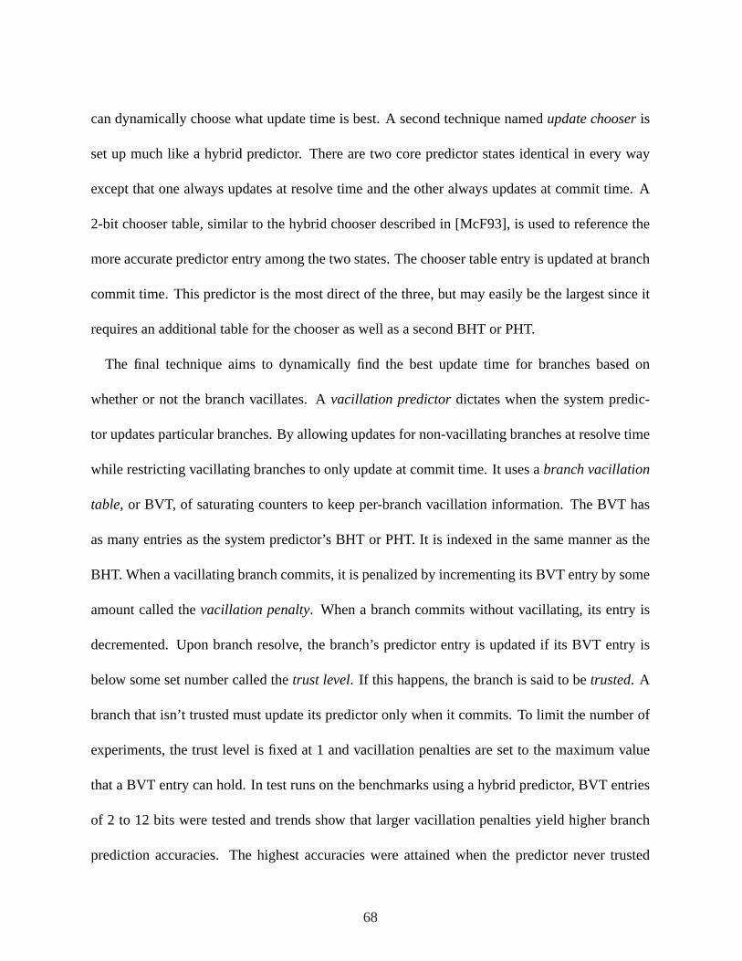
can dynamically choose what update time is best. A second technique namedupdate chooseris
set up much like a hybrid predictor. There are two core predictor states identical in every way
except that one always updates at resolve time and the other always updates at commit time. A
2-bit chooser table, similar to the hybrid chooser described in [McF93], is used to reference the
more accurate predictor entry among the two states. The chooser table entry is updated at branch
commit time. This predictor is the most direct of the three, but may easily be the largest since it
requires an additional table for the chooser as well as a second BHT or PHT.
The final technique aims to dynamically find the best update time for branches based on
whether or not the branch vacillates. Avacillation predictordictates when the system predic-
tor updates particular branches. By allowing updates for non-vacillating branches at resolve time
while restricting vacillating branches to only update at commit time. It uses abranch vacillation
table, or BVT, of saturating counters to keep per-branch vacillation information. The BVT has
as many entries as the system predictor’s BHT or PHT. It is indexed in the same manner as the
BHT. When a vacillating branch commits, it is penalized by incrementing its BVT entry by some
amount called thevacillation penalty. When a branch commits without vacillating, its entry is
decremented. Upon branch resolve, the branch’s predictor entry is updated if its BVT entry is
below some set number called thetrust level. If this happens, the branch is said to betrusted. A
branch that isn’t trusted must update its predictor only when it commits. To limit the number of
experiments, the trust level is fixed at 1 and vacillation penalties are set to the maximum value
that a BVT entry can hold. In test runs on the benchmarks using a hybrid predictor, BVT entries
of 2 to 12 bits were tested and trends show that larger vacillation penalties yield higher branch
prediction accuracies. The highest accuracies were attained when the predictor never trusted
68

-0.5
0
0.5
1
1.5
Bim
odal
0
0.4
0.8
1.2
Wea
keni
ng Im
pact
GS
hare
0
0.3
0.6
gzip swim vpr.p vpr.r gcc art mcf craftyfacerec
parserperl gap bzip2
twolfmesa
Hyb
rid
changestatic
chooservacillation
Figure 6.10: Misprediction Rate Impact of Flexible Update Schemes (petdis.90,103,104,106);Results are shown as the increase in misprediction rate from a system updating predictors atcommit time.
vacillating branches. This is accomplished by using a 1 bit-per-entry BVT initialized to 0. If a
branch vacillates, its BVT entry is set to 1 and it will not be trusted for the rest of execution. This
is the way in which the vacillating predictor used in this study is configured.
6.3.6 Performance of Flexible Update Schemes
Each of the proposed techniques was simulated on a static snipper system. The results for each
flexible update method with bimodal, GShare, and hybrid predictors are shown in Figure 6.10.
Results are presented as the increase in misprediction rate from updating at commit time, and
updating atchangehas been added for comparison.
For the bimodal predictor, almost all benchmarks favor thecommit update method overchange.
69

-0.2
0
0.2
0.4
0.6
0.8
1
1.2
1.4
1.6
gzip swim vpr.p vpr.r gcc art mcf craftyfacerec
parserperl gap bzip2
twolfmesa
Diff
eren
ce in
Mis
pred
ict R
ate
Benchmark
c.c.bi-c.ud.bis.c.bi-s.ud.bi
s.c.bi-c.c.bi
Figure 6.11: Analysis of Bimodal Chooser (petdis.90,111); Results shown as differences in mis-prediction rates of several systems.
The static and chooser flexible update techniques perform better than the base snipper system,
reducing the misprediction rate by around 0.2. The vacillation predictor does not perform better
than the regular system predictor.
Precisely answering the question of how much delayed update weakening can be avoided is
difficult when examining the behavior of correlating predictors because they are affected by
mangled-path weakening as well. Recall that the only type of weakening that affects systems
with bimodal predictors is delayed-update weakening. Because it performs best, the amount of
weakening that the flexible update chooser can reduce will now be analyzed in detail.
Call a conventional system that uses a bimodal predictor that updates at commitc.c.bi and
70
the same system that uses a bimodal update chooser predictorc.ud.bi. Call a snipper system that
uses a bimodal predictor that updates at commits.c.bi and one that uses a bimodal update chooser
s.ud.bi. The improvement of the misprediction rate for the bimodal chooser on a conventional
system isRc.c.bi − Rc.ud.bi. Likewise, the improvement for a snipper system isRs.c.bi − Rs.ud.bi.
The bimodal weakening impact isRs.c.bi − Rc.c.bi. These three differences are represented in
Figure 6.11 by the first, second, and third results for each benchmark respectively.
The first result in the figure shows that even a conventional system benefits from the chooser
flexible update predictor. Among the benchmarks that benefit are the ones most affected by
update lag in the bimodal predictor in Figure 6.5. Snipper benefits more from the update chooser
than the conventional system, as shown by 11 of the 15 benchmarks. The difference between
the first two results is a reasonable measurement of the amount of alleviated delayed-update
weakening. Compare this difference to the last result, which shows the total weakening. In four
cases, vpr.place, vpr.route, crafty, and parser, the update chooser alleviated almost all weakening.
In 4 benchmarks there were more minor reductions in weakening.
Because it cannot be easily isolated from mangled-update weakening, it is not as easy to mea-
sure the amount of alleviated delayed-update weakening for GShare and hybrid predictors. How-
ever, a good estimation can be provided using the classification of Figure 6.3. Towards the end
of the study, when providing results for a CIP-aware predictor, this estimated measurement will
be presented.
71
6.4 Mangled-Path Weakening
6.4.1 Description
Since true CDR outcomes are not known to post-reconvergent branches until after prior protected
branches resolve, it is impossible to obtain a correct GHR to predict CI instructions in a CIP.
Mangled path weakening is weakening caused by differences in paths from a conventional system
to a CIP.
Call the bits in a GHR corresponding to the CDR thepadded region. In a conventional system
the padded region would consist of the correct outcomes of the CDR branches. In a CIP they
are at best a guess, and so mangle the GHR. There are two ways in which a CIP mangles the
GHR. First, the number of outcome history bits in the padded region, called thepad size, may
not match the number of branches in the correct CDR. If the padded region is too small, noise
may be brought in at the fringe and cause branch predictor training time to increase. If it’s too
large, useful correlation data could be pushed out at the fringe and cause weakening due to lack of
correlation data. The other way in which the GHR is mangled is the contents of the padded region.
Since the true CDR outcomes cannot be used,outcome history paddingschemes that inject false
histories into the path at special times in execution are used. A common technique involves
padding with predicted CDR outcomes, even though they may be incorrect. This provides a best
guess, but may not be the best way to minimize weakening.
Definefringe noise ingestionto occur when noisy branch outcomes are brought into the global
history that would otherwise not appear on a conventional system.Fringe signal lossoccurs
when useful data is pushed out of the GHR. DefineCDR signal lossto occur when the padded
region lacks important correlation data it would otherwise have in a conventional system. Finally,
72

CDR noise ingestionoccurs when incorrect CDR outcomes not containing valuable correlation
data cause weakening. These are the causes of mangled-path weakening.
A dynamic CIP can turn protection on and off and therefore change the padded region from
the correct CDR outcomes to predicted CDR outcome bits, or even to no bits at all. Consider
a dynamic CIP that does not put outcomes in the padded region when protecting a branch. If
protection of the branch turns on and off during execution, subsequent branches may suffer from
all the afore mentioned types of mangled-path weakening. A static CIP that does not include
outcomes in its padded region can only suffer from fringe noise ingestion and CDR signal loss.
The weakening that fringe noise ingestion causes is referred to asexternal insulated weaken-
ing. Likewise, fringe signal loss causessoft absentee weakening, CDR signal loss causeshard
absentee weakening, and CDR noise ingestion causesinternal insulated weakening. Recall, since
true CDR outcomes are simply not available when protecting a branch in a CIP, hard absentee
weakening cannot be avoided.
6.4.2 Examples
On a system using GShare, the branch at address0x1a950 from the SPEC CPU 2000 bench-
mark crafty is a simple yet effective example of internal insulated weakening. The branch’s
misprediction rate rises by 10% when using snipper. Throughout the majority of execution, the
branch is highly biased not-taken. Observation of the system state shows that the branch’s GHR
often contains outcomes from misspeculated paths at predict time. This causes the branch to be
associated with more table entries and hence exhibit a longer training time.
A system with a Hybrid predictor is used in the following example. In the art benchmark,
the branch at address0x12fbc is the top weakened branch of the benchmark, doubling in mis-
73

CD
Correct GHR
TTTTTTTTTTTTTTTUsed GHR
0x13054
Mispredicted
TTTTTTTNTTNTTTT
Figure 6.12: GHR State for Branch0x12fbc
A
CD Region
B
C
D
E
A
CD Region
B
C
D
E
True PathObserved Path
Figure 6.13: Control Flow Graphs of Two Separate Executions
predictions when using snipper. In areas of execution, the branch exhibits a very stable local
history ofTTTTTTTTTTNcontinuously. The GHR is too small to reflect this entire pattern with
nearby global outcomes; however, this branch is highly correlated to another branch at address
0x13054 . Figure 6.12 shows that the correct outcome of the correlated branch is not reflected in
the GHR when using Snipper, since the CD path taken does not contain it. This exemplifies one
case of hard absentee weakening in which a branch is weakened when correlation data within the
CD region is unavailable due to a misprediction of the incident branch.
74

6.4.3 Path Splitting and Joining
Because CIPs fetch out of program order, observed paths of correlating predictors may not nec-
essarily be true paths. Refer to the first control flow graph of Figure 6.13 which shows a control
flow graph of a certain area in a program leading to the basic blockA. Only the basic blocks
of paths leading toA are shown. Assume that the branch inB is highly correlated to the one in
D and thatD has been marked for protection. The true paths are marked along with observed
paths in a CIP. Assume that a conventional system will always fetchA through the control path
EDCB. Notice that there are two ways in which the CIP fetchesA, EDCB andEDB. The
latter is not a true path yet is still an observed path containing the CD region where the protected
branchD is mispredicted.
If the branch predictor of a CIP uses predicted CDR branch outcomes for the GHR’s padded
region, both control pathsEDB andEDCB are observable fromA even though only one of
them is a true path. This is an example of how paths may besplit. Since each path corresponds to
a PHT entry and each entry requires some amount of training, splitting paths typically increases
the training time of branches.
Paths may also bejoined. The second control flow graph in Figure 6.13 shows two possible
true paths through the region. Assume that in this case the branch inB is no longer correlated
to the one inD. A conventional system will observe both of these control paths,EDCB and
EDB, in execution. A CIP that does not include CD data in its path, however, will only observe
one path through this region. This is an example of how paths may be joined.
Define the union∪ of two path filtered local histories,L1 andL2, to be the combined local
history of the paths’ outcomes arranged in program order. Consider two systems,X andY . A
75

path-filtered local history on systemX, LX , is said to beperfectly splitinto LYi , for all 0 ≤ i < n
for some integern, such that the following holds.
Perfect Path Splitting:LX =⋃
0≤i<n
LYi (6.6)
Path filtered local historiesLXi , for all 0 ≤ i < n are said to beperfectly joinedif there exists a
path filtered local historyLY on systemY such that the following holds.
Perfect Path Joining:LY =⋃
0≤i<n
LXi (6.7)
Realistically, perfect path splitting is expected to happen rarely. A more common case is when a
path filtered local history splits into paths that contain outcomes from other paths.
Path Splitting:LX ⊆⋃
0≤i<n
LYi (6.8)
To avoid overcomplicated analysis, only the perfect path joining and perfect path splitting models
are discussed for the remainder of this chapter. It is realized, however, that this is not always the
case.
Figure 6.14 shows examples of how paths may split or joined. The horizontal lines denote the
bias of the path filtered local history with respect to time. A higher line indicates a taken outcome
while a lower line indicates a not-taken outcome. The outcomes are marked for each point in time
the branch reached by the path resolves. The shaded region denotes an inevitable misprediction.
Assume that the update lag is low enough such that there are no delayed update mispredictions
76

LA
L
L
B
B
1
2 LB
L
1
2
A
A
L
T T T T T T
TimePath Splitting
T
Path Joining
T T
TT T
T T T
T T T T T T TT N NNT
N N
N NN N
NNN
N N N N N N
N N N N N N
Figure 6.14: Examples of Path Splitting and Joining
and assume no predictor collisions.
The left side of the figure shows how a path may be split from one system to another. The
bistable path above the line is split into the two separate bistable paths shown below the line.
Note that the amount of mispredictions go from two to four. The right side of the figure shows
how two bistable paths in one system may be joined in another system. Since the bias of the two
shown paths are usually not similar, the number of mispredictions rises substantially when the
paths are joined. The different causes of path splitting and joining will be articulated as well as
some performance implications for each.
Thus far, it has been shown how path splitting and joining can hurt performance, but this is
not always the case. Consider two separate paths of a conventional system, both highly biased
taken. Each path suffers two training mispredictions since they each have a separate predictor
entry to train. If the path in some system is modified to join these two original paths so that they
share a PHT entry, then the amount of training mispredictions is halved. This example shows that
77

CDR
Worst Case
CDR
Slight Case
TTNNNNTT
TTNNNNTT
TTTTNNNN
TTNNNNTT
TTNNNNTT
NNTTNNNN
NTTTNNNN
TNTTNNNN
TTTTNNNN
Figure 6.15: Examples of External Insulated Weakening
even conventional systems may benefit from modification of the way the PHT is indexed, though
studying this in detail is beyond the scope of the thesis.
Causes of Mangled Path Weakening
All proposed CIPs either predict post-reconvergent branches using the predicted CDR outcomes
or completely leave these outcomes out of the GHR. To exemplify the different types of mangled
path weakening, first consider a CIP that leaves CDR data out of the path. The GHR samples
markedSlight Casein Figure 6.15 show the GHR of one path for some post-reconvergent biased
branch in a conventional system being split into two paths on a CIP. The first split path is ob-
served when a candidate branch (whose outcome is the first in the marked CDR) is not protected
yet. This path is identical to the true path of the conventional case. The last split path is that
of the branch when it is a post-reconvergent region of some earlier protected branch that has yet
to resolve. Notice that since the CDR outcomes are no longer present in the history (marked by
a dotted underline), two more distant outcomes appear (not underlined). This is an example of
fringe noise ingestion. The external insulated weakening in this case will be the added mispre-
dictions for the training of this new path. TheWorst Caseexample shows that ingestion of noisy
branches can add a considerable amount of mispredictions The two outcomes brought in at the
fringe are noisy, and so the original path is split into four separate paths, each of which will suffer
78
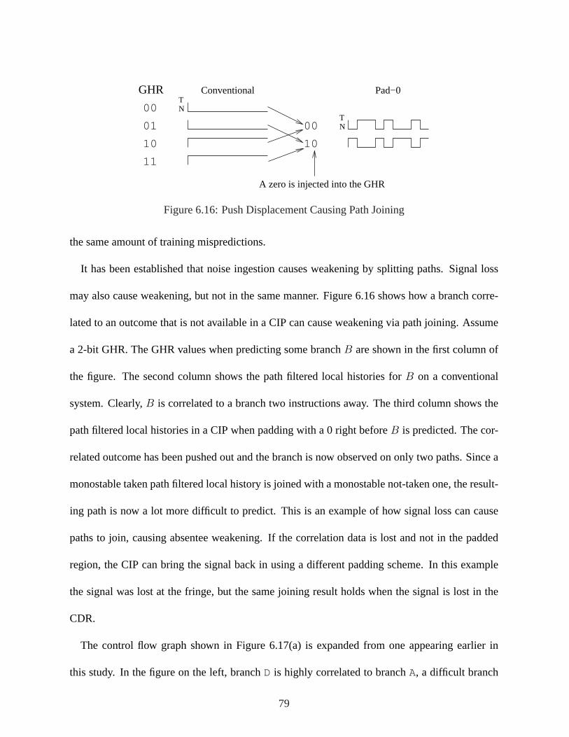
00
01
10
11
TN
00
10
TN
A zero is injected into the GHR
ConventionalGHR Pad−0
Figure 6.16: Push Displacement Causing Path Joining
the same amount of training mispredictions.
It has been established that noise ingestion causes weakening by splitting paths. Signal loss
may also cause weakening, but not in the same manner. Figure 6.16 shows how a branch corre-
lated to an outcome that is not available in a CIP can cause weakening via path joining. Assume
a 2-bit GHR. The GHR values when predicting some branchB are shown in the first column of
the figure. The second column shows the path filtered local histories forB on a conventional
system. Clearly,B is correlated to a branch two instructions away. The third column shows the
path filtered local histories in a CIP when padding with a 0 right beforeB is predicted. The cor-
related outcome has been pushed out and the branch is now observed on only two paths. Since a
monostable taken path filtered local history is joined with a monostable not-taken one, the result-
ing path is now a lot more difficult to predict. This is an example of how signal loss can cause
paths to join, causing absentee weakening. If the correlation data is lost and not in the padded
region, the CIP can bring the signal back in using a different padding scheme. In this example
the signal was lost at the fringe, but the same joining result holds when the signal is lost in the
CDR.
The control flow graph shown in Figure 6.17(a) is expanded from one appearing earlier in
this study. In the figure on the left, branchD is highly correlated to branchA, a difficult branch
79

A
A Resolves
B
D
E
G H
C C’ F
(a) (b)
A
A Resolves
B
C
D
E
F
G H
CD Region
CI Region
CD Region
CI Region
Figure 6.17: Control Flow Example for CDR Juggling
to predict. The branchH, a monostable branch, will be reached from two control paths in a
conventional system, eitherABDEGor ACDFG. As described before, H will be reached from two
additional paths in a CIP that uses CDR outcomes to predict,ACDEGandABDFG. Though there
haven’t been any outcomes pulled in or pushed out of the GHR, the incorrect CDR outcomes can
still cause weakening since each of these paths needs to train in the predictor. This is an example
of how noise ingestion in the CDR can cause internal insulated weakening.
Because different paths through the CDR may vary in the number of branches per path, internal
insulated weakening may occur in tandem with soft absentee weakening or external insulated
weakening. Figure 6.17(b) shows a CFG which adds another branchC’ to one of the paths
through the CDR. In a CIP, the control pathABDEGpath is split intoABDEGandACC’DEG.
Since the latter path contains more outcomes than the true path, fringe signal loss, and hence
soft absentee weakening, becomes possible. This shows that different types of mangled-path
weakening may occur in tandem.
Since path splitting and joining can improve performance, the way in which CIPs mangle paths
can help branch prediction accuracy. It is evident, however, that it usually hurts more than helps
[HR07].
To help bring a general understanding to how a CIP changes true paths, certain path statistics
80

0
5
10
15
20
25
30
gzip swim vpr.p vpr.r gcc art mcf craftyfacerec
parserperl gap bzip2
twolfmesa
Sta
tic P
ath
Rat
e
Benchmark
Static Path Rate for Several Systems
ConventionalSnipper pad-nullSnipper pad-cdr
Figure 6.18: Static Path Rate for Several Systems (petdis.111)
81

are measured and evaluated. The results are gathered using a predictor that analyzes pure 16-bit
paths and is collision-free. Define thestatic path rateas the total number of static paths seen
in this configuration divided by the static instruction count. The division is performed to scale
results better for clarity of Figure 6.18. Shown in the figure is the path rate for a conventional
system, a snipper system that does not use outcome history padding (pad-null), and a snipper
system that pads with predicted CDR outcomes (pad-cdr). Note that these path results are meant
to give a quick look into snipper’s behavior under different padding schemes. It is not intended
to provide any major conclusions, since it does not reveal anything about the manner in which
the static paths are used or branch prediction accuracy for the paths.
The results carry a notion that snipper, whether it’s using pad-null or pad-cdr, tends to split
paths. Extreme increases in the static path rate from the conventional system to snipper pad-null,
like those of crafty, parser, and bzip, gives a clue that noise ingestion may be a factor (remember,
this is static snipper). In almost every case, padding with the predicted CDR outcomes further
increases the total number of static paths. The parser and bzip2 benchmarks actually have fewer
static paths in snipper pad-cdr than snipper pad-null. These benchmarks seem to split paths by
ingestion at the fringe much more than by ingestion in the CDR.
6.4.4 The Effect of Path Splitting and Path Joining
Path splitting and joining from a conventional system to a CIP have the potential of causing
considerable amounts of weakening. To get a notion of how drastic the weakening could be, a
model is developed that demonstrates simple cases of splitting and joining. Equations presented
in this section assume no update lag.
Assume a path filtered local history with a constant number of outcomes per run. Assume the
82

number of outcomes per run is considerably large. Also assume that the initial PHT entry value,
0 or 3, will cause a misprediction, and that there are no collisions. Call the number of runs in
the historyφ. Let L(i) represent thei’th outcome of the path filtered local historyL. Assume
that historyLX is split into two paths,LY1 andLY
2 such that any outcomeLX(i) occurs in the
new pathLYS(i), whereS models the way in which the path is split. SetS to be a random variable
representing a Bernoulli trial. This models a scenario near what the worst case split would be.
The number of mispredictions of the path filtered local historyLX is 2φ, since each run will
have two training mispredictions. The number of mispredictions of each pathLY1 andLY
2 is
also 2φ. The total number of mispredictions for the original pathLX doubled in the system
where it has split. The weakening due to the modeled path splitting is then2φ additional training
mispredictions.
Bistable path split :WX,Ysplit (L) = MX(LX) (6.9)
The model corresponds to some path in a conventional system that suffers from one bit of noise
ingestion, where the noisy branch’s outcome is random. This one unwanted bit in the GHR can
cause a considerable amount of weakening, doubling the amount of training mispredictions for
the original path. Indeed, the amount of mispredictions with respect to the amount of ingested
noisy bits rises exponentially. Thankfully, the large majority of applications do not contain large
amounts of noisy branches.
Assume two highly biased path filtered local historiesLX1 andLX
2 . Two cases are analyzed for
the joining of two paths. For the first one, assume that pathsLX1 andLX
2 are each monostable
unanimous. These paths are joined to form the historyLY such thatLY (i) occurs inLXS(i) for all
outcomesi. Here, the two monostable paths have joined into one monostable path. This causes
83

MLYfewer mispredictions in the systemY .
For the second case, assume thatLX1 andLX
2 are monostable dissonant. Since the signals
oppose each other, the joining of these paths causes a tremendous amount of weakening. Instead
of using the Bernoulli trial to join the two paths, assume the paths will be joined by interdigitation
so thatLY (i) is taken fromLXi%2. Joining the paths in this way will causei/2 mispredictions.
Monostable dissonant path join:WX,Yjoin (LX
1 , LX2 ) = i/2 (6.10)
Though the modeled cases for Equation 6.9 and Equation 6.10 probably do not happen often,
they demonstrate near worst cases on the amount of weakening a path join or split may cause.
6.4.5 Outcome History Padding
Recall that since the padded region in a CIP can not consist of the correct CDR outcomes, the
outcome history padding method becomes important. There are two main issues of CIPs that
cause mangled path weakening. First, the size of the outcome history padding not matching
the size of the conventional padded region. This may cause external insulated weakening and
soft absentee weakening. The second issue deals with the contents of the padded region and
may cause internal insulated weakening and hard absentee weakening. The following padding
schemes are designed to address these issues.
One method mentioned several times in this study ispad-null. When using this method there
is no outcome history used for padding. CDR outcomes and are left out entirely and no false
histories are injected. Using this padding method is favorable if there usually aren’t noisy out-
comes ingested at the fringe. This technique eliminates internal insulated weakening in static
CIPs, though it may increase the amount of external insulated weakening in doing so.
84

Including predicted CDR outcome data is another method mentioned many times earlier in this
study. It is referred to aspad-cdr. This method is the only one we present that may cause internal
insulated weakening due to CDR juggling. However, post-reconvergent branches may attain
higher accuracies when correlating to incorrect predicted CDR outcomes rather than nothing at
all. Additionally, if the different paths through the CDR have a similar amount of branches, the
padding size of this method could effectively prevent fringe effects.
A very simple padding scheme calledpad-0 is the one shown in Figure 6.16. Though it has
a negative context in the figure, it has the potential to reduce weakening in CIPs by pushing
noisy outcomes out of the fringe, which prevents path splitting. Padding similarly with two
zero bits as opposed to one is calledpad-00, and padding with three is calledpad-000. The
pad size can be customized for each static protected branch.pad-0avguses the padding size for
each protected branch as set by a profile. For our purposes, the profile sets the pad size to the
average number of CDR outcomes for an entire reference input run of the branch’s benchmark.
This technique, calledfitted padding, provides insight to how dynamically changing the padding
size could help padding performance. Padding schemes that use it are suffixed with -avg. This
naming convention is used for all the remaining padding methods. For this padding method and
all remaining methods, the maximum static pad size is fixed at 3. This number has been chosen
by examining the average number of branches in the CDRs of snipper-active benchmarks. This
number ranges from 1 to 3.3, with the average being 2. Due to its potential complexity, study
of changing the amount of padding bits for each protected branch beyond fitted padding is not
studied here.
Padding with zeros may reduce mangled path weakening by removing noise from the fringe but
85
may cause unwanted path joining since it causes less variance across all paths. To prevent this, the
pad-cmethod pads with the reconvergent branch’s address bits instead of just zero bits. The bits
are taken starting at the third least significant bit and going in the direction of more significance.
For example, pad-ccc will pad the GHR with the third, fourth, and fifth least significant bits of
the PC. This method allows post-reconvergent instructions to correlate with protected branches
rather than their outcomes. The padding bits have been chosen intuitively to increase the chances
that two nearby protected branches will pad with different values.
The pad-cdrmethod defined earlier differs from methods proposed so far in that it doesn’t
consistently use the same pad size for static protected branches in execution. If the number of
branches in different CDR paths of the same static branch varies greatly,pad-omay be a better
option. This method hashes the CDR outcomes to a constant pad size. Since some correla-
tion data may be lost, some hashing algorithms may be more optimal than others. The hashing
algorithm used for this study is fixed as the following.
s_cdr = number of branches in the CDRs_pad = pad sizecdr[s_cdr] = sequence of CDR outcomes, index 0 is most recentpad[s_pad] = 0for i from 0 to (s_cdr DIV s_pad)
pad = pad XOR cdr[i:i+s_pad]
The : operator in the pseudo code above represents a slice and indexing starts from 0. For
example,cdr[3:5] is a 3-bit number consisting of the fourth, fifth, and sixth bits ofcdr
respectively. The padding size, number of branches in the CDR, and sequence of CDR outcomes
are all given initially. After completion of the algorithm, the variablepad contains the padding.
This algorithm was designed as a very simple approach. The padding is constructed byXORing
consecutive segments of the CDR outcomes until all of them have been operated on. For the last
86

Table 6.2: Padding MethodsName Padding Variations Pad Sizepad-null No padding None Fixedpad-cdr Predicted CDR outcomes None Variablepad-0 0 pad-00, pad-000 Fixedpad-0avg 0 Variablepad-c Reconvergent Branch’s Address pad-cc, pad-ccc Fixedpad-cavg Reconvergent Branch’s Address Variablepad-o Hash of predicted CDR outcomespad-oo, pad-ooo Fixedpad-cavg Hash of predicted CDR outcomes Variable
segment, zeros are used as padding if there are not enough outcomes to fill the entire segment.
Table 6.2 shows a summary of all the different padding types explored in this study.
6.5 Performance of Outcome History Padding Schemes
All of the padding schemes presented above have been simulated and analyzed for each of the
benchmarks. Of all three static padding sizes of those schemes with them, a padding size of 3
yields the best branch prediction ratio on average, followed by a padding size of 2, then 1. The
fitted padding methods perform nearly as well as their 3-bit counterparts. The results for all the
padding schemes of interest are shown in Figure 6.19 for GShare and Figure 6.20 for hybrid.
For clarity, the results are shown as the increase in misprediction rate from the pad-null scheme.
Graphs of collision rates are appended help give insight as to why some padding schemes are
outperforming others.
The GShare predictor is generally more sensitive to the padding schemes than the hybrid pre-
dictor. The best case improvement in misprediction rate with GShare is about 0.7 whereas with
hybrid it’s nearly 0.2. Of all the benchmarks, twolf is the only one that responds negatively to
the developed padding schemes, it performs best with pad-null. On average, the pad-ccc scheme
outperforms the rest, with pad-cavg being a close second. The collision results appended to the
87

-1
-0.5 0
0.5 1
1.5 2
Increased Mispredict RateGShare
-5-4-3-2-1 0 1 2 3 4 5
gzip
swim
vpr.p
vpr.r
gcc
art
mcf
craf
tyfa
cere
cpa
rser
perl
gap
bzip
2tw
olf
mes
a
Increased Collision RateGShare
pad-
cdr
pad-
0pa
d-00
pad-
000
pad-
0avg
pad-
cpa
d-cc
pad-
ccc
pad-
cavg
pad-
opa
d-oo
pad-
ooo
pad-
oavg
Figure 6.19: Misprediction Rate and Collision Impact of Padding Schemes for the GShare Pre-dictor (petdis.137); Results are shown as the increase in misprediction rate from a system usingpad-null.
88

-0.2 0
0.2
0.4
0.6
0.8 1
1.2
Increased Mispredict RateHybrid
-4-3-2-1 0 1 2 3 4 5
gzip
swim
vpr.p
vpr.r
gcc
art
mcf
craf
tyfa
cere
cpa
rser
perl
gap
bzip
2tw
olf
mes
a
Increased Collision RateHybrid
pad-
cdr
pad-
0pa
d-00
pad-
000
pad-
0avg
pad-
cpa
d-cc
pad-
ccc
pad-
cavg
pad-
opa
d-oo
pad-
ooo
pad-
oavg
Figure 6.20: Misprediction Rate and Collision Impact of Padding Schemes for the Hybrid Pre-dictor (petdis.137); Results are shown as the increase in misprediction rate from a system usingpad-null.
89

graph give insight as to why this could be. Collision results for pad-c techniques are typically
less than those of other techniques, especially pad-o which tends to drive the predictor to more
collisions.
90

Chapter 7
Measurement by Weakening Type
The previous chapter formally defined several types of weakening. Here, techniques for measur-
ing interesting subsets of the weakening types will be described. Measurement of weakening is
important since it sheds light on where efforts in reducing weakening should be spent. Moreover,
it helps assess how effective a reduction technique is for its targeted weakening type.
7.1 Approach
Finding the reason that a dynamic branch is weakened in the CIP is difficult, mainly because it’s
hard to isolate the outcomes to which a branch is correlated. A practical approach to classify
weakened branches is to examine the performance of system pairs chosen so that only one or a
few weakening types occur from one chosen system to the other. The estimated breakdown of
weakening by type shown in Figure 6.3 is constructed in this way. For example, a static CIP
using pad-null can be compared to another that uses pad-cdr. It has already been established that
weakening from the former system to the latter is mainly internal insulated weakening, external
insulated weakening, and soft absentee weakening, all of which can be improved by padding
methods.
The first system in themodel system walkwill be a conventional system and the last will be
a snipper system. Intermediate systems will be modeled to isolate desired subsets of weakening
for eachstepin the walk. The weakening from one step to the next will then be a measurement of
some subset of weakening, and the sum of the weakening of every step will be the total weakening
when going from a conventional system to a snipper system. Keep in mind that the intermediate
91

modeled systems may not be useful other than to collect this information.
Though measuring each weakening type is difficult, the systems were able to be modeled such
that important subsets of weakening are measured. The targeted weakening types are as follows.
In the study of mangled-update weakening earlier in the text, it was established that systems
with a bimodal predictor mainly suffered from delayed-update weakening when predictors up-
date at commit. Because it has not been measured for GShare and hybrid predictors, the first
targeted weakening subset is delayed update weakening. To find the amount of weakening that
is unavoidable when performing protected recovery, the second subset is hard absentee weak-
ening. Other types of weakening presented here may be remedied by outcome history padding
schemes, so soft absentee weakening, internal insulated weakening, and external insulated weak-
ening comprise the last targeted subset. A way to measure each of these three types of weakening
individually has not yet been developed.
7.2 Model Systems
Each modeled system of the walk is named with a tuple in which components are separated
by a dot. The first item of the tuple indicates the type of execution, either conventional (c) or
snipper (s), while the second indicates the type of padding. The model systems use a 64ki-entry
hybrid predictor. The other parameters of the model systems’ configuration meet those shown in
Table 5.1.
The first system,c.cdr, is a conventional system.
The second,c.o, sets the padded region to a hash of true outcomes (in the same manner as
pad-o) but there is no protected recovery. Because post-reconvergent branches are squashed
on a protected misprediction, there is no re-execution for post-reconvergent instructions. This
92

eliminates nearly all of the update lag that snipper induces. Upon protecting a branch, this system
pads the GHR with a hash of true CDR outcomes when it reaches the reconvergence point. In
order to provide as much correlation data as possible, the pad size is customized to each static
protected branch using fitted padding. This technique is used so that branches with larger CDRs
are less likely to lose CDR correlation data in the hash. The purpose of the c.o system is to make
CDR outcomes available for the protected branch’s post-reconvergent instructions while padding
with a consistent number of bits. Since there should only be a small amount of hard absentee
weakening (because most CDR outcomes will be available in the pad) and no delayed update
weakening (because there is no speculative execution), the weakeningW c.cdr,c.o is predominantly
due to external insulated weakening and soft absentee weakening.
The systemc.c is similar to c.o except that the GHR is padded with PC bits (like pad-cavg) as
opposed to true CDR outcomes. The pad size for each protected branch matches exactly to that
of the c.o system. This way, there is no insulated weakening or soft absentee weakening between
the two systems. The weakeningW c.o,c.c is therefore due to hard absentee weakening.
The next system,s.c, uses snipper to perform protected recoveries. This means that the post-
reconvergent instructions will be predicted earlier relative to the predicted branch that causes
delayed-update weakening. The padding scheme is exactly the same as that of c.c. Therefore,
W c.c,s.c is due to delayed-update weakening.
The final system,s.null, is a snipper system that uses the pad-null method. Because the system
does not insert outcomes into the padded region,W s.c,s.null is due to fringe noise ingestion.
A summary of the modeled systems are listed as follows along with the behavior of Post-
Reconvergent Branches (PRBs).
93
c.cdr: PRBs use true path and do not execute speculatively.
c.o: PRBs have access to most correct CDR outcomes, do not execute speculatively, andare reached by slightly mangled paths.
c.c: PRBs do not have access to CDR outcomes, do not execute speculatively, and arereached by slightly mangled paths.
s.c: PRBs do not have access to CDR outcomes, execute speculatively, and are reached byslightly mangled paths.
s.null: PRBs do not have access to CDR outcomes, execute speculatively, and are reachedby mangled paths.
This classification is by no means presented as a be-all end-all measurement. On the contrary,
this is only the first measurement of the presented weakening types and there may be plenty of
room for improvement. Weakening measured by some pairs are expected to be more accurate
than others. As mentioned before,W c.cdr,c.o may contain small amounts of hard absentee weak-
ening, as outcomes may be lost in the hash. The hashing algorithm used may not be the best to
prevent outcomes from being lost. Since there may be small amounts of absentee weakening in
W c.cdr,c.o, the measurement of hard absentee weakening,W c.o,c.c, may not cover the actual ab-
sentee weakening of the system. The measurement of delayed-update weakening is expected to
be fairly accurate, since there is only very little protection overhead in the c.c system it behaves
much like a conventional one as far as predictor update timings are concerned.
7.3 Results
The results in Figure 7.1 show the weakening for each step of the model system walk from a
conventional system to a pad-null snipper system. Note that the weakening is negative for some
system pairs. Recall from earlier in the text that many of the behaviors that generally cause
weakening may increase branch prediction accuracy in some cases. As the figure shows, this
phenomenon is rare and is of very little magnitude when it does occur in most cases.
94

-0.5
0
0.5
1
1.5
2
c.cdr, c.oc.o, c.c
c.c, s.cs.c, s.null
Wea
keni
ng R
ate
System Pair
gzipswimvpr.pvpr.rgccart
mcfcrafty
facerecparser
perlgap
bzip2twolf
mesa
Figure 7.1: Weakening Among Model Systems (petdis.109)
95

The classification of Figure 6.3 was generated in the following way. Delayed update weak-
ening isW c.c,s.c, hard absentee weakening isW c.o,c.c, and soft absentee and external insulated
weakening areW c.cdr,c.o + W c.c,s.null. These classes are marked as mangled update, mangled
path, and absentee in the figure. Some of these classes of weakening were measured as negative.
This is expected since, as discussed earlier, the effects that cause weakening can also increase
branch prediction accuracy. In generating the classification, these negative weakening results are
factored out of the final percentage.
96
Chapter 8
CI Aware Branch Predictor
The majority of branch weakening is from CIP side-effects that may be reduced by using special
branch predictor techniques. It has been shown that flexible update schemes can reduce signifi-
cant amounts of delayed-update weakening for a CIP using the bimodal predictor while outcome
history padding can improve branch prediction accuracy in the CIP. Now, the first CI Aware
branch Predictor, or CIAP (pronouncedchap), is presented. It will be implemented based on the
presented weakening alleviation techniques based on their performance and ease of implementa-
tion.
8.1 Implementation
The branch predictor is designed to use the flexible update chooser and pad-ccc outcome history
padding scheme with the hybrid predictor as a core. Since this study does not consider the cost of
predictor size, enabling the flexible update chooser will cause the predictor to more than double
the size of its Hybrid counterpart. In order to compensate for this cost, results are compared
against conventional systems with a hybrid flexible update chooser. Outcome history padding
has a relatively low cost on the design.
The CIAP with a Hybrid core will use two PHTs, two BHTs, and one chooser table, all of
which have 2-bit entries. One hybrid predictorstate, consisting of a PHT, BHT, and chooser, will
update at change while the other will update at commit. A chooser, which is always updated at
commit time, will choose one state just as described in Section 6.3.5. The predictor is configured
to have 64ki entries and use a 16-bit GHR.
97

0.5
1
1.5
2
2.5
Wea
keni
ng R
ate
0.9
1
1.1
1.2
1.3
1.4
gzip swimvpr.p vpr.r gcc art mcf craftyfacerec
parserperl gap bzip2
twolfmesa
Spe
edup
Update ChooserSnipper
CIAPpad-cccCIAPpad-cavg
Figure 8.1: Performance of Hybrid CIAP (petdis.123); Results are shown as the increase inweakening rate and speedup from a conventional system with a hybrid predictor. The snippersystem shown uses pad-null.
8.2 Results
A breakdown of the speedup and weakening rate results of several systems including snipper with
the CIAP are shown in Figure 8.1. Note, all of the results in this particular figure are captured for
dynamic snipper. Weakening results are measured from a conventional system with a regular hy-
brid predictor to the respective system labeled in the figure. The first result shows the weakening
rate and speedup for a conventional system outfitted with an update chooser. The performance is
expected to slightly increase in this case, but not dramatically since conventional systems are less
susceptible to update lag. The second result is for a snipper system. The system is configured
with pad-null for outcome history padding and a regular hybrid predictor that updates at commit
98

time. The third result is for snipper with the CIAP described earlier in the chapter, referred to
as CIAPpad-ccc. A CIAP predictor that uses pad-c with fitted padding called CIAPpad-cavg has
been added as the last result to provide a slightly more complex CIAP for comparison.
The flexible update predictor significantly improves the conventional branch prediction accu-
racy in the conventional case for 5 out of the 15 benchmarks. In only two of these benchmarks
does this value equal the improvement in branch prediction accuracy from a snipper system to the
CIAP system, meaning flexible update has helped eliminate some mangled-update weakening.
The CIAPpad-ccc predictor reduced weakening for 12 of the 15 benchmarks. The CIAP was
able to reduce weakening enough to cause 3 benchmarks originally slowed down by snipper to
exhibit speedup.
Of the 3 benchmarks that benefit greatly from snipper, 2 suffer more weakening using the
CIAPpad-ccc as opposed to using a hybrid predictor with pad-null. Both of these benchmarks,
gzip and twolf, do not react well to any of the weakening reduction techniques presented in this
study. However, in both of these cases CIAPpad-cavg predictor maintains speedup very close to
that of snipper. CIAPpad-cavg outperforms CIAPpad-ccc in 4 of the benchmarks, and performs
nearly as well in most others.
Even with the unfavorable results of gzip and twolf, both CIAP predictors improve speedup
and reduce weakening on average across all of the benchmarks. The CIAPpad-ccc improves
speedup by0.015 and reduces the weakening rate by0.114misp/kI. The CIAPpad-cavg im-
proves speedup by0.019 and reduces the weakening rate by0.022misp/kI.
To find the different types of weakening the CIAP has eliminated, refer to Figure 8.2. This
is the measurement of weakening presented in the previous chapter for snipper outfitted with
99
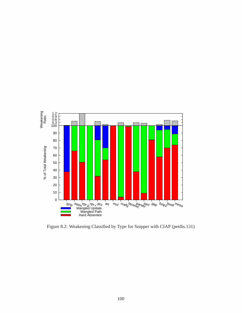
0.3 0.6 0.9 1.2
Wea
keni
ngR
atio
0
10
20
30
40
50
60
70
80
90
100
gzip swimvpr.p vpr.r gcc art mcf craftyfacerec
parserperl gap bzip2
twolfmesa
% o
f Tot
al W
eake
ning
Hard AbsenteeMangled Path
Mangled Update
Figure 8.2: Weakening Classified by Type for Snipper with CIAP (petdis.131)
100

CIAPpad-ccc. Comparing this figure with Figure 6.3, the measurement shows that mangled-
update weakening has been eliminated completely in 4 benchmarks that originally suffered from
it in a snipper system with a hybrid predictor and the pad-null scheme. Mangled-path weakening
has either been eliminated or greatly reduced in three of the benchmarks.
101

Chapter 9
Conclusion and Future Work
Branch weakening has been formalized and defined by its several causes. In doing so, this study
has revealed that some types of weakening may be eliminated while others are inherent to control
independence and cannot be avoided. Study of branch behaviors and branch predictors in both
conventional systems and control independence processors enabled a thorough understanding of
why branches are weakened. Through development of a classification that measures the several
types of weakening, it has been established that the majority of weakening may be remedied by
using special branch prediction techniques that reduce update lag and path mangling. Among
the techniques that work best and are easy to implement, the CIAP has been introduced. This
branch predictor uses fundamental weakening reduction techniques to eliminate weakening and
does so successfully. Of all 15 benchmarks, 12 exhibited less weakening. Three benchmarks that
were originally slowed down by snipper using a hybrid predictor and the pad-null method exhibit
speedup with the CIAP.
The techniques used to reduce weakening that are presented in this study are among the most
fundamental. Though a considerable amount of weakening has been reduced using these tech-
niques, there is opportunity to explore more robust techniques and examine a larger parameter
space.
Internal absentee weakening cannot be avoided when the branch inducing the weakening is
marked for protection. Many current CIPs including snipper dynamically turn protection on and
off in execution, but none of them consider this type of weakening when doing so. Detection of
102

a weakened branch in execution is feasible. A second predictor state that predicts and updates
its GHR and tables at commit time can be used to compare against the system predictor. This
commit-time predictoris not useful for predicting branches (since it predicts them too late), but
can be used to detect weakening since it operates very similarly to a predictor in a conventional
system. If the system predictor mispredicts a branch and the commit-time predictor yields a
correct prediction, the branch instance may be marked as weakened. Though not discussed in
this paper, a commit-time predictor has been used in this research to find examples of weakened
branches for study. Though using this technique is a good way to dynamically detect weakened
branches, finding the protected recovery that caused the weakening is a hard problem and has not
been explored.
The mangled-path weakening reduction techniques offered in this thesis may be greatly im-
proved upon. In many cases the pad-avg techniques show that one padding size certainly does
not fit all. Padding schemes where the padding size dynamically changes in execution is not ex-
plored in great detail here, but is a good problem for future research since the results of the CIAP
show that there is a lot of mangled-path weakening to be dealt with.
Because the base system of study used here updates at commit time, update shuffling and
incorrect update have not been studied in detail. Though employing the CIAP eliminates delayed-
update weakening for most benchmarks, it does so with a very aggressive technique that doubles
predictor size. The vacillation predictor has a large parameter space could be explored much
more rigorously in a more focused study.
Finally, techniques in classification can be developed for each distinctive type of weakening.
Also, dynamic classification techniques may be developed in the future that classify weakened
103

branch mispredictions on the fly as opposed to using the postmortem model system approach.
This could allow for greater performance by employing particular weakening reduction tech-
niques to particular situations.
104

Bibliography
[ARM] Arm8. http://infocenter.arm.com/help/index.jsp.
[AZRRA07] Ahmed S. Al-Zawawi, Vimal K. Reddy, Eric Rotenberg, and Haitham H.Akkary. Transparent control independence (tci).SIGARCH Comput. Archit. News,35(2):448–459, 2007.
[CFS99] Yuan Chou, Jason Fung, and John Paul Shen. Reducing branch mispredictionpenalties via dynamic control independence detection. InICS ’99: Proceedings ofthe 13th international conference on Supercomputing, pages 109–118, New York,NY, USA, 1999. ACM.
[CPT08] Bumyong Choi, Leo Porter, and Dean M. Tullsen. Accurate branch prediction forshort threads. InASPLOS XIII: Proceedings of the 13th international conferenceon Architectural support for programming languages and operating systems, pages125–134, New York, NY, USA, 2008. ACM.
[CTW04] Jamison D. Collins, Dean M. Tullsen, and Hong Wang. Control flow optimizationvia dynamic reconvergence prediction. InMICRO 37: Proceedings of the 37thannual IEEE/ACM International Symposium on Microarchitecture, pages 129–140, Washington, DC, USA, 2004. IEEE Computer Society.
[CV01] Chen-Yong Cher and T. N. Vijaykumar. Skipper: a microarchitecture for exploit-ing control-flow independence. InMICRO 34: Proceedings of the 34th annualACM/IEEE international symposium on Microarchitecture, pages 4–15, Washing-ton, DC, USA, 2001. IEEE Computer Society.
[DR95] Kaivalya Dixit and Jeff Reilly. Spec95 questions and answers.SPEC Newsletter,7(3):7–11, 1995.
[EM98] A. N. Eden and T. Mudge. The yags branch prediction scheme. InMICRO 31:Proceedings of the 31st annual ACM/IEEE international symposium on Microar-chitecture, pages 69–77, Los Alamitos, CA, USA, 1998. IEEE Computer SocietyPress.
[FRB01] Brian Fields, Shai Rubin, and Rastislav Bodk. Focusing processor policies viacritical-path prediction. InIn Proceedings of the 28th Annual International Sym-posium on Computer Architecture, pages 74–85, 2001.
[GF00] Jayanth Gummaraju and Manoj Franklin. Branch prediction in multi-threadedprocessors. Inin Proceedings of the 2000 International Conference on ParallelArchitectures and Compilation Techniques, pages 179–188, 2000.
[GKMP98] Dirk Grunwald, Artur Klauser, Srilatha Manne, and Andrew Pleszkun. Confidenceestimation for speculation control. InIn 25th Annual International Symposium onComputer Architecture, pages 122–131, 1998.
105

[Hen00] John L. Henning. Spec cpu2000: Measuring cpu performance in the new millen-nium. Computer, 33(7):28–35, 2000.
[HP03] John L. Hennessy and David A. Patterson.Computer Architecture, A QuantitativeApproach. Morgan Kaufmann Publishers, San Fransisco, CA, US, 2003.
[HP08] John L. Hennessy and David A. Patterson.Computer Organization and Design.Morgan Kaufmann Publishers, San Fransisco, CA, US, 2008.
[HPRA02] Christopher J. Hughes, Vijay S. Pai, Parthasarathy Ranganathan, and Sarita V.Adve. Rsim: Simulating shared-memory multiprocessors with ilp processors.Computer, 35(2):40–49, 2002.
[HR07] Andrew D. Hilton and Amir Roth. Ginger: control independence using tag rewrit-ing. In ISCA ’07: Proceedings of the 34th annual international symposium onComputer architecture, pages 436–447, New York, NY, USA, 2007. ACM.
[HSF00] Michael Haungs, Phil Sallee, and Matthew Farrens. Branch transition rate: Anew metric for improved branch classification analysis. InIn Proc. HPCA, pages241–250, 2000.
[JKL00] Daniel A. Jimenez, Stephen W. Keckler, and Calvin Lin. The impact of de-lay on the design of branch predictors. InMICRO 33: Proceedings of the 33rdannual ACM/IEEE international symposium on Microarchitecture, pages 67–76,New York, NY, USA, 2000. ACM.
[JL01] Daniel A. Jimenez and Calvin Lin. Dynamic branch prediction with percep-trons. InHPCA ’01: Proceedings of the 7th International Symposium on High-Performance Computer Architecture, page 197, Washington, DC, USA, 2001.IEEE Computer Society.
[JRS96] Erik Jacobsen, Eric Rotenberg, and J. E. Smith. Assigning confidence to con-ditional branch predictions. InMICRO 29: Proceedings of the 29th annualACM/IEEE international symposium on Microarchitecture, pages 142–152, Wash-ington, DC, USA, 1996. IEEE Computer Society.
[JSHP97] Stephan Jourdan, Jared Stark, Tse-Hao Hsing, and Yale N. Patt. Recovery require-ments of branch prediction storage structures in the presence of mispredicted-pathexecution.Int. J. Parallel Program., 25(5):363–383, 1997.
[KG99] Artur Klauser and Dirk Grunwald. Instruction fetch mechanisms for multipathexecution processors. InIn MICRO-32, pages 38–47, 1999.
[Kop02] David M. Koppelman. The benefit of multiple branch prediction on dynamicallyscheduled systems. InWorkshop on Duplicating, Deconstructing, and Debunkingheld in conjunction with the 29th International Symposium on Computer Architec-ture, pages 42–51, 2002.
106
[Kop08] David M. Koppelman. Lsu ece technical report 2008-dmk-1. Department of Elec-trical and Computer Engineering, Louisiana State University, 2008.
[Loh06] G.H. Loh. Revisiting the performance impact of branch predictor latencies.IEEEInternational Symposium on Performance Analysis of Systems and Software, 0:59–69, 2006.
[LW92] Monica S. Lam and Robert P. Wilson. Limits of control flow on parallelism.SIGARCH Comput. Archit. News, 20(2):46–57, 1992.
[McF93] Scott McFarling. Combining branch predictors.WRL TN-36, 1993.
[MS90] Steven S. Muchnick and Richard Schell. Sun’s compiler technology. pages 69–70,1990.
[PSEa] Pse. http://www.ece.lsu.edu/koppel/pse/.
[PSEb] Viewable simulation batch data sets for pse. http://svn.ece.lsu.edu/ds/cjm/.
[PT09] Leo Porter and Dean M. Tullsen. Creating artificial global history to improvebranch prediction accuracy. InICS ’09: Proceedings of the 23rd internationalconference on Supercomputing, pages 266–275, New York, NY, USA, 2009. ACM.
[RJS99] Eric Rotenberg, Quinn Jacobson, and Jim Smith. A study of control independencein superscalar processors. InIn HPCA-5, pages 115–124, 1999.
[RSI] Rsiml. http://www.ece.lsu.edu/koppel/work/proc.html.
[SBV95] Gurindar S. Sohi, Scott E. Breach, and T. N. Vijaykumar. Multiscalar processors.In In Proceedings of the 22nd Annual International Symposium on Computer Ar-chitecture, pages 414–425, 1995.
[SI94] CORPORATE SPARC International, Inc.The SPARC architecture manual (ver-sion 9). Prentice-Hall, Inc., Upper Saddle River, NJ, USA, 1994.
[Sit93] Richard L. Sites. Alpha axp architecture.Commun. ACM, 36(2):33–44, 1993.
[SMC00] Kevin Skadron, Margaret Martonosi, and Douglas W. Clark. A taxonomy ofbranch mispredictions, and alloyed prediction as a robust solution to wrong-historymispredictions. InIn Proceedings of the 2000 International Conference on Paral-lel Architectures and Compilation Techniques, page pages, 2000.
[Smi81] James E. Smith. A study of branch prediction strategies. InISCA ’81: Proceed-ings of the 8th annual symposium on Computer Architecture, pages 135–148, LosAlamitos, CA, USA, 1981. IEEE Computer Society Press.
[SPHC02] Timothy Sherwood, Erez Perelman, Greg Hamerly, and Brad Calder. Automati-cally characterizing large scale program behavior. pages 45–57, 2002.
107

[Sto01] Jon Stokes. The pentium 4 and the g4e: an architectural comparison: Part i.http://arstechnica.com/old/content/2001/05/p4andg4e.ars/4, 2001.
[Sto06] Jon Stokes. Into the core: Intel’s next-generation microarchitecure.http://arstechnica.com/hardware/news/2006/04/core.ars/, 2006.
[TDF+02] J. M. Tendler, J. S. Dodson, J. S. Fields, H. Le, and B. Sinharoy. Power4 systemmicroarchitecture.IBM J. Res. Dev., 46(1):5–25, 2002.
[yCHyYP94] Po yung Chang, Eric Hao, Tse yu Yeh, and Yale Patt. Branch classification: a newmechanism for improving branch predictor performance. InIn Proceedings of the27th International Symposium on Microarchitecture, pages 22–31, 1994.
[YP92] Tse-Yu Yeh and Yale N. Patt. Alternative implementations of two-level adaptivebranch prediction. InIn Proceedings of the 19th Annual International Symposiumon Computer Architecture, pages 124–134, 1992.
[YP93] Tse-Yu Yeh and Yale N. Patt. A comparison of dynamic branch predictors that usetwo levels of branch history. Inin Proceedings of the 20th Annual InternationalSymposium on Computer Architecture, pages 257–266. ACM, 1993.
[YS99] Cliff Young and Michael D. Smith. Static correlated branch prediction.ACMTransactions on Programming Languages and Systems, 21:1028–1075, 1999.
108

Vita
Christopher J. Michael was born in Kuwait in 1980. His father is of Iraqi-Turkish ethnicity and
his mother is of Palestinian-Lebanese ethnicity. He has lived in Baton Rouge, Louisiana since
1982. Among his academic interests are computer architecture, high performance computing,
and application development in performance analysis. In the non-academic domain, he enjoys
playing his oud and cooking various vegetable, mineral, and animal. He will receive his doctorate
in electrical engineering from Louisiana State University in May of 2010. After graduation, he
will be conducting post-doctoral research at the Naval Research Lab, Stennis Space Center.
109