the water footprint of india - universiteit twenteessay.utwente.nl/537/1/scriptie_kampman.pdf ·...
TRANSCRIPT

The water footprint of India
Doeke Kampman
The water footprint of India
A study on water use in relation to the consumption of
agricultural goods in the Indian states
Master thesis
Date: April 2007
Author: D.A. Kampman
Email: [email protected]
Graduation committee: Prof. Dr. Ir. A.Y. Hoekstra (University of Twente)
Dr. Ir. M.S. Krol (University of Twente)


“As I travel around the world, people think the only place where there is potential
conflict over water is the Middle East, but they are completely wrong. We have the
problem all over the world. “
(Koffi Annan)
“When the well is dry, we learn the value of water”
(Benjamin Franklin)

Preface
The completion of this study means the completion of the Master course Civil Engineering &
Management at the University of Twente.
I started with the execution of this study in May 2006. After a good start, I got stuck on the
many decisional crossroads this subject has to offer and I slowly realised that this study might
not shake up the world as much as I had hoped. However, after making some rough
decisions, I began to see the light and things started to fall into place. In the last period of this
study, I have tried hard to write a comprehensible report on the subject, including a relevant
link to the Indian society. And although there is still room for improvements, I am very
satisfied with the current result.
I would like to thank a number of people without whom this result would not have been
possible.
First of all, I would like to thank the members of my graduation committee. I would like to
thank Arjen Hoekstra for his advice, criticism and ideas, for helping me with the overall
direction of the study and for offering me a look in the interesting kitchen of multidisciplinary
water management. I would like to thank Maarten Krol for his profound analysis of my
concept reports, which undoubtedly increased the scientific value of the study. I would like to
thank both Arjen Hoekstra and Maarten Krol for the pleasant collaboration during the
execution of this study.
I also would like to thank Ashok Chapagain for his sharing his knowledge on the subject.
Next, I would like to thank my colleagues at the graduation chamber for their pleasant
company, for the discussions in the coffee corner and for sharing the good times and “de uren
van nood en ontbering” with me.
I also would like to thank my parents for creating a steady base in this life for me, for their
advice and for their ever present support.
Finally, I would like to thank Rianne for her love, faith and encouragement. Although from a
long distance during the weeks, her support has been immensely important to me.
Doeke Kampman
Enschede, April 2007
Acknowledgement This study has been executed at the University of Twente under the department of Water
Engineering & Management between May 2006 and April 2007. I would like to thank the
department of Water Engineering & Management for offering me the necessary facilities
during this period.


Summary
The concept of the water footprint has been developed to create an indicator of water use in
relation to the consumption by people. The water footprint of a country is defined as the
volume of water needed for the production of the goods and services consumed by the
inhabitants of the country. The water footprint is divided into a blue, a green and a gray
component. The blue component refers to the evaporation of groundwater and surface water
during the production of a commodity, the green component to the evaporation of rain water
for crop growth, and the gray component to the water required to dilute the water pollution
that is caused by the production of the commodity to acceptable levels.
In the next fifty years, India is projected to face the challenge of feeding a population of 1.6
billion people with a higher level of welfare than at present. The current view of the Indian
government on food security is to hold on to the goal of food self sufficiency. Knowing that
agriculture is the main consumer of water, the implied increase in food demand will increase
the pressure on the renewable water resources.
In order to reduce the pressure on renewable water resources, the Indian government is
considering the concept of river interlinking as the solution for water scarcity in the drier
regions. This concept means that water abundant regions will provide water to water scarce
regions through the connection of rivers. Whether the interlinking of rivers will provide
enough water to solve the observed and future water deficit and what the side effects of the
project will be is still unclear.
This study indicates why the water scarce regions have a water deficit. In the period 1997-
2001, the water footprint of the inhabitants of the Indian states varied between 451 and 1357
m3/cap/yr with an average of 777 m3/cap/yr. Of this average, 658 m3/cap/yr originated from
local water resources and 119 m3/cap/yr from water resources of other states or other nations.
Furthermore, the blue component of the average water footprint came to 227 m3/cap/yr, the
green component to 459 m3/cap/yr and the gray component to 92 m3/cap/yr.
During the study period, the total virtual water flow as a result of interstate trade in
agricultural commodities in India was 106 billion m3/yr, which was 13% of the total water use
in Indian agriculture. In the same period, the net international export from India was 15
billion m3/yr. Of the total virtual water flow within India, 35% was due to the interstate trade
in milled rice, 17% due the interstate trade in raw sugar and 14% due to the interstate trade in
edible oils. The largest interregional net virtual water flow was 22 billion m3/yr and flowed
from North India to East India. As a result of international and interstate virtual water flows,
the states Haryana, Madhya Pradesh, Punjab and Uttar Pradesh had the largest net export of
virtual water and Bihar, Jharkhand and Kerala had the largest net import of virtual water.
The water scarcity from the perspective of consumption is the highest in the states of
Rajasthan, Punjab, Uttar Pradesh, Tamil Nadu and Haryana. This means that the water
resources of these states are closest to be exhausted in case of food self sufficiency. Because
most of the states are also net exporters of virtual water, the water scarcity from production
perspective is even higher in these states.
The total net global water saving as a result of the interstate trade in agricultural commodities
in India was 41 billion m3/yr. This means the total water use in Indian agriculture was 5%

lower than it would have been without interstate trade. The interstate trade in wheat alone
already caused a global water saving of 23 billion m3/yr.
Looking at the river interlinking project from the perspective of the virtual water flows as
calculated in this study, it can be seen that the proposed water transfer from East to North
India has a direction exactly opposite to the direction of the virtual water flow as a result of
interstate trade. In this study, it is demonstrated that an increase in water productivity in the
water abundant states has a better chance of reducing the national water scarcity than the
proposed water transfer. The river interlinking project mainly reduces local water scarcity,
while water scarcity needs to be reduced significantly at a national level in order to remain
food self sufficient as a nation. The only long term option for reducing the national water
scarcity and remaining food self sufficient is to increase the water productivity in India. The
largest opportunity for this increase lies in East India, where there is an abundance of water
and a large increase in water productivity seems possible.


Table of Contents
1. Introduction .................................................................................................................... 1
1.1 Background of the study .......................................................................................... 1 1.2 The virtual water concept ......................................................................................... 2 1.3 The water footprint concept ..................................................................................... 2 1.4 The water saving concept ......................................................................................... 3 1.5 Objectives .................................................................................................................... 3
2. Methodology .................................................................................................................. 5 2.1 Overview .................................................................................................................... 5 2.2 Calculation of virtual water content ....................................................................... 5
2.2.1 Crop water requirement .................................................................................... 5 2.2.2 Green crop water use ......................................................................................... 6 2.2.3 Blue crop water use ............................................................................................ 8 2.2.4 Dilution water requirement .............................................................................. 9 2.2.5 Virtual water content ....................................................................................... 10 2.2.6 Virtual water content of processed products................................................ 10 2.2.7 Water productivity ........................................................................................... 11 2.2.8 Water use ........................................................................................................... 11
2.3 Calculation of virtual water flows ......................................................................... 11 2.3.1 National and state crop balance ..................................................................... 11 2.3.2 Interstate trade .................................................................................................. 12 2.3.3 Virtual water flows........................................................................................... 14
2.4 Calculation of the water footprints ....................................................................... 15 2.5 Estimation of water resources ................................................................................ 16
2.5.1 Water balance of a state ................................................................................... 16 2.5.2 Internal water resources of a state ................................................................. 17 2.5.3 External water resources of a state ................................................................. 18
2.6 Assessment of water scarcity ................................................................................. 19 2.6.1 Water scarcity from production perspective ................................................ 19 2.6.2 Water scarcity from consumption perspective ............................................. 20
2.7 Calculation of water saving ................................................................................... 20 2.7.1 Global water saving ......................................................................................... 20 2.7.2 Water saving and the theory of comparative advantage ............................ 21 2.7.3 Relative water saving ....................................................................................... 21
3. Study scope and data collection ............................................................................... 23
3.1 Study area ................................................................................................................. 23 3.2 Crop coverage .......................................................................................................... 25 3.3 Data collection .......................................................................................................... 27
3.3.1 Climatic parameters ......................................................................................... 27 3.3.2 Crop parameters ............................................................................................... 28 3.3.3 Irrigated area fraction ...................................................................................... 28 3.3.4 Dilution water requirement ............................................................................ 28 3.3.5 Product and value fractions of crops ............................................................. 29 3.3.6 Population ......................................................................................................... 29 3.3.7 National crop balance ...................................................................................... 29 3.3.8 Crop area, production and yield .................................................................... 30 3.3.9 Crop consumption ............................................................................................ 31 3.3.10 Interstate trade .................................................................................................. 32 3.3.11 Water resources ................................................................................................ 33

4. Virtual water content of crops................................................................................... 35 4.1 Virtual water content of the primary crops ......................................................... 35 4.2 Virtual water content of milled rice ...................................................................... 36 4.3 Comparison with other studies ............................................................................. 37
5. Interstate and interregional virtual water flows.................................................... 39 5.1 Interstate and international product trade ........................................................... 39 5.2 Interstate virtual water flows ................................................................................. 40 5.3 Interregional virtual water flows .......................................................................... 42
6. Water footprints ........................................................................................................... 45
6.1 Water footprints of the Indian states .................................................................... 45 6.2 Water footprint by colour ....................................................................................... 48 6.3 Water footprint by crop .......................................................................................... 49 6.4 Water footprint by region ....................................................................................... 49 6.5 Water scarcity ........................................................................................................... 50 6.6 Global water saving as a result of interstate trade .............................................. 51 6.7 Water saving as a result of comparative advantage in water productivity ..... 54
7. Food security: River interlinking versus increasing water productivity .......... 59 7.1 Strategies for Indian water management ............................................................. 59 7.2 River interlinking project........................................................................................ 60 7.3 Increasing water productivity ............................................................................... 61
7.3.1 Potential yield ................................................................................................... 61 7.3.2 Potential global water saving ......................................................................... 62
7.4 River interlinking versus increasing water productivity ................................... 65 7.4.1 Potential reduction of water scarcity ............................................................. 65
7.5 Water saving by changing crop patterns .............................................................. 68 8. Conclusion and discussion ........................................................................................ 71
8.1 Conclusion ................................................................................................................ 71 8.2 Discussion ................................................................................................................. 72
References .............................................................................................................................. 75
Appendices
I Symbols
II Area and Population of the Indian states
III Crop production India
IV List of weather stations
V Crop parameters
VI Product and value fractions
VII National crop balances
VIII Virtual water contents of crops
IX Comparison of calculated gray water use to nitrate use by state
X Sensitivity analysis of virtual water content of kharif milled rice
XI Production, consumption and surplus of crops
XII Assessment of interstate and international crop trade
XIII Interstate virtual water flows by colour
XIV Water footprints by colour
XV Water footprints compared to consumption volume and climate
XVI Other estimates on the water resources of India
XVII Average annual precipitation
XVIII Water resources of the Indian states
XIX Blue water flows between the Indian states
XX Assessment of water scarcity in a potential situation


1
1. Introduction
1.1 Background of the study
With over one billion people, India currently has the world’s second largest population. The
estimate of the amount of people living in India in the year 2050 is 1.6 billion (United Nations,
2004). This is an increase in population of approximately 50% in the next fifty years. Next to
this population growth the total Gross Domestic Product (GDP) per capita in India is also
growing rapidly (7.1% in 2005 (World Bank, 2006)). Furthermore, there currently is a net
export of agricultural products from India, which has shown an increase in the past decade
(FAO, 2006a), which is likely to persist. These developments will lead to a large growth in the
total food demand in India in the near future.
How can India cope with this scenario? Can the production of food be increased? And if so,
should India increase its food production or should India import more products from other
countries?
Since most of the utilizable water supply in India is used for crop production (Hoekstra &
Chapagain, 2007), an important criterion for the evaluation of a possible food supply strategy
is the pressure on renewable water resources. At the moment there are regions in India that
are determined as water scarce, as the water availability per is capita is less than 1000 m3/yr,
which is either caused by the lack of natural water resources or a result of over exploitation of
groundwater resources for irrigation purposes (CGWB, 1989; Bobba et al., 1997).
The pressure on water resources is also increasing through the increase in water pollution
caused by diffuse agricultural sources in the form of animal manure, fertilizers and pesticides.
While the application of fertilizers and pesticides is currently low compared to developed
countries, the intensification of agriculture is bound to cause an increase of diffuse
agricultural pollution. The monitoring of groundwater and surface water have currently only
resulted in the reporting of high nitrate concentrations in groundwater, which is in most cases
linked directly to diffuse agricultural sources (Agrawal, 1999).
The current point of view of the Indian government on the topic of food security is to hold on
to the goal of national food self sufficiency. The begging bowl image of the sixties is
something that is still carved in the minds of the Indian people and is to be prevented at all
cost (Gupta & Deshpande, 2004; Planning Commission, 2002).
In order to reduce the pressure on the renewable water resources, the Indian government is
considering the concept of river interlinking as the solution for water scarcity in the drier
regions. This concept means that water abundant regions will provide water to water scarce
regions through the connection of rivers (NWDA, 2006). Whether the interlinking of rivers
will provide enough water to solve the water deficit and what the side effects of the project
will be is still unclear (Radhakrishna, 2003).

Water footprint of India Introduction
2
Since the interlinking of rivers is such an enormous project, it is useful to see to what extent
another strategy can reduce the water scarcity in the drier regions.
1.2 The virtual water concept
This other water scarcity reducing strategy can be quantitatively described with the concept
of virtual water. This concept defines the virtual water content of a commodity as the volume
of water that is actually used to produce the commodity, measured at the place where the
commodity is actually produced (Allen, 1993, 1994). The inverse of the virtual water content is
known as the water productivity of a crop.
With the virtual water content, the production and the trade flow of a crop can be translated
into the water use and the virtual water flow of crop. So instead of increasing local water
resources by importing water, the water use in the water deficit regions can be reduced by an
increase in water productivity or a change in the existing trade pattern. The water
productivity of a crop can be increased when a significant gap exists between the current and
potential water productivity. A change in the existing trade pattern is possible if importing
states can increase their crop production and can be become less dependent, self sufficient or
even exporters.
1.3 The water footprint concept
In line with the concept of virtual water, the concept of the water footprint has been
introduced to create a consumption-based indicator of water use (Hoekstra & Hung, 2004;
Hoekstra & Chapagain, 2007). This in contrast to the traditional production-sector-based
indicators of water use, that are useful in water management but do not indicate the water
that is actually needed by the inhabitants of a country in relation to their consumption
pattern. The water footprint is defined as the volume of water needed for the production of
the goods and services consumed by the inhabitants of a country. This concept is developed
in analogy to the concept of the ecological footprint (Wackernagel & Rees, 1996).
The water footprint can be divided into an internal and an external water footprint. The
internal component covers the use of domestic water resources and the external component
covers the use of water resources elsewhere.
Furthermore, an agricultural, an industrial and a domestic component of the water footprint
can be assessed. Here, the agricultural component corresponds with the water use in the
agricultural sector (i.e. in the form of crop evapotranspiration or water pollution), the
industrial component corresponds with the water use in the industrial sector and the
domestic component with the water use in the domestic sector.
Finally, the water footprint can be divided into a blue, a green and a gray water footprint. The
blue component covers the use of groundwater and surface water during the production of a
commodity, the green component covers the use of rain water for crop growth, and the gray
component covers the water required to dilute the water that is polluted during the
production of the commodity. The distinction between green and blue water has been
introduced by Falkenmark & Rockström (1993). The gray component has been introduced by
Chapagain et al. (2006).

Water footprint of India Introduction
3
1.4 The water saving concept
With the current water productivity in India and the food demand scenario for the year 2050,
it seems inevitable for India to become an importer of virtual water (Falkenmark, 1997; Yang
et al., 2003; Falkenmark & Lannerstad, 2005). This is because the average (utilizable) water
availability per capita in India will drop below the minimum amount of water needed to feed
a person in the near future. This means that water scarcity is not only a local problem in India
but also a national problem.
Given that the total water resources are more or less fixed, neglecting possible climatic
changes, the only way to reduce the national water scarcity is to reduce the total water use
with a constant or growing food production. This means that an increase in water
productivity is needed together with water saving on a global scale.
Global water saving is created when a product that is traded has a higher virtual water
content in the importing state than in the exporting state (Chapagain & Hoekstra, 2006). This
means that the water loss in the exporting state is lower than the water saving in the
importing state. If the water loss as a result of trade is larger than the water saving, there is a
global loss.
1.5 Objectives
To get more insight on whether the water scarcity in the Indian states is caused by local
consumption or by the export of agricultural commodities to other states or countries, the
water footprints of the Indian states are assessed in this study.
The first target of this study is to assess the international and interstate virtual water flows
from and to the Indian states and create a net virtual water balance for each state. In order to
assess these virtual water flows, the import, export and virtual water contents of the crops
need to be calculated for each Indian state. Because data on crop trade is not directly available
at the state level, the trade of a crop is estimated based on the production and consumption
volumes per state and the national balance of a crop.
The second target is to assess the water footprints related to the consumption of agricultural
commodities of the Indian states. This is determined by the water use in the states and the
virtual water flows from and to the states.
The third target is to assess the water scarcity in the Indian states. To this end, the water
resources are estimated by state. Water scarcity is assessed from the production perspective
by comparing water availability to the water use in a state, and from the consumption
perspective by comparing water availability to the water footprint of a state.
The fourth target is to assess global water saving as a result of interstate trade in agricultural
commodities. Global water saving is calculated from the difference between the virtual water
content of the crop in the importing and exporting state. Global water saving gives an
indication of the relative water use efficiency of interstate trade in agricultural commodities in
India.
The fifth and last target of this study is to compare the river interlinking project to the
outcome of the previous objectives. This might give an indication to what extent the local and
national water scarcity can be reduced more by water transport through the connection of
Water footprint of India Introduction
4
rivers or by a combination of an increase in water productivity and a change in interstate
trade patterns.
The period of analysis in this study is 1997-2001, because this is the most recent five-year
period for which all necessary data could be obtained. The scope of the study is limited to
agricultural commodities, since they are responsible for the major part of global water use
(Postel et al., 1996). Livestock products are not taken into account, because they are more
difficult to assess and generally contribute a small part to the total trade in virtual water
(Chapagain & Hoekstra, 2003).

5
2. Methodology
2.1 Overview
The starting point in this methodology is the calculation of the green, blue and gray virtual
water content of a crop by season and by state. This calculation is derived from a method
used by Chapagain et al. (2006). The following step is the estimation of the international and
interstate trade of a crop by state. This estimation is based on the method used by Ma et al.
(2006). With the virtual water contents, the crop production of a state is translated into the
water use of a state and the interstate crop trade of a state into the virtual water flow of a
state. The total water use and the gross virtual water flows of a state determine the water
footprint of a state. Next, the water resources of the Indian states are estimated. Together with
the water footprint, the water resources give an indication of the water scarcity in the Indian
states. Finally, the global water saving as a result of interstate trade is calculated.
Throughout this chapter, independent variable c denotes crop, s state, t time steps of 10 days,
p agricultural product, rb river basin and us upstream state. A summary of all used symbols in
this study is presented in Appendix I.
2.2 Calculation of virtual water content
2.2.1 Crop water requirement
The calculation of the virtual water content of a crop starts with the calculation of the volume
of water that is required for the crop growth.
Crop water requirement (CWR, m3/ha) is defined as the volume of water that is required to
compensate the water loss of a crop through evapotranspiration under growth conditions
with no constraint by water shortage (Allen et al., 1998).
The CWR is calculated by accumulating the data on the crop evapotranspiration under
optimal conditions (ETc,opt, mm/day) over the complete growing period.
[ ] [ ]tscETscCWRlp
t
optc ,,10,1
,∑=
∗= (1)
Here, the factor 10 is included to convert mm into m3/ha and the summation is done in time
steps of 10 days over the full growing period lp. It is worth noticing that in this calculation
each month is taken to be equal to 3 time steps of 10 days, which means that all months are
assumed to consist of exactly 30 days.
The ETc, opt is calculated as follows:

Water footprint of India Methodology
6
[ ] [ ] [ ]sETcKscET ocoptc ∗=,, (2)
In this equation, Kc is the crop coefficient (-) and ET0 is the reference evapotranspiration in a
state (mm/day). Because neither ET0 nor Kc is constant over the growing period, ETc,opt is
calculated for every time step of 10 days over the full growing period.
The reference evapotranspiration ET0 is defined as the evapotranspiration rate from a
hypothetical grass reference crop with specific characteristics, which has an abundance of
water. Because of the abundance of water available for evapotranspiration at the reference
surface, soil factors can not form a constraint for the ET0 rate. This means that ET0 only
expresses the evaporating power of the atmosphere at a specific location and time of the year
and does not consider a difference in crop characteristics and soil factors. Therefore ET0 is
computed with climatic data.
The crop coefficient Kc determines how ETc,opt from a certain crop field relates to ET0 from the
reference surface. The major factors that determine Kc are crop variety, climate and crop
growth stage. During the various growth stages of a crop the value of Kc changes, because the
ground cover, the crop height and the leaf area change as the crop develops.
The total growing period is divided into four growth stages: the initial stage, the crop
development stage, the mid-season stage and the late season stage (Allen et al, 1998). The
initial stage is the period from the planting date to approximately 10% ground cover. The crop
development stage is the period from 10% ground cover to effective full cover. The mid-
season stage is the time from effective full cover to the time the crop starts to mature. The late
season is the final stage and is the time from the start of maturity to harvest. The total Kc curve
of a crop is shown in Figure 2.1.
2.2.2 Green crop water use
The green crop water use (CWUgreen) is the volume of the total rainfall that is actually used for
evapotranspiration by the crop field (m3/ha) and is calculated by accumulating the data on
crop evapotranspiration under rain fed conditions (ETc,rw, mm/day) over the complete
growing period.
Crop growing season (days)
Crop development stage Mid-season stage Late season stageInitial stage
Kc ini
Kc mid
Kc end
Figure 2.1: Development of Kc during the crop growing season (Chapagain & Hoekstra, 2004).

Water footprint of India Methodology
7
[ ] [ ]tscETscCWUlp
t
rwcgreen ,,*10,1
,∑=
= (3)
As in the calculation of the CWR, the factor 10 is included to convert mm into m3/ha and the
summation is done over the full growth period lp (day) in time steps of 10 days.
The ETc,rw is determined as follows:
[ ] [ ] [ ]),,(, ,, sPscETMinscET effoptcrwc = (4)
Here, Peff is the effective rainfall (mm/day), which is defined as the amount of the total
precipitation (Ptot, mm/day) that can be used for evapotranspiration by the crop and the soil
surface.
Equation 4 shows that ETc,rw is equal to Peff if Peff is lower than ETc,opt, and that ETc,rw is equal to
ETc,opt if Peff is higher than ETc,opt. This is because a crop uses as much water as possible for
ETc,opt, but never uses more water than it requires for optimal growth. The fact that in some
time steps a part of the Peff is not used for evapotranspiration, and is thus still available as soil
moisture for a following time step, is not taken into account in this study.
The effective rainfall Peff is generated from Ptot by CROPWAT (FAO, 2006b). CROPWAT
calculates with a simplified version of the USDA method. This is a simplification because the
soil type and the net depth of irrigation application are not taken into account in this method
(Dastane, 1978). The simplified method consists of equations 5 and 6. The factor 30 is added to
these equations, because the original equations assume monthly values instead of daily
values. The relation between Peff and Ptot that is created by these equations is presented in
Figure 2.2.
)2.030
125(
125
30
30
250tottotefftot PPPP ∗−∗∗=→≤ (5)
totefftot PPP ∗+=→> 1.030
125
30
250 (6)
0
1
2
3
4
5
6
7
8
9
10
0 1 2 3 4 5 6 7 8 9 10
Total rainfall (mm/day)
250/30 ≈ 8.3Ptot
Peff
Eff
ect
ive
rain
fall
(m
m/d
ay)
Figure 2.2: The relation between effective rainfall and total rainfall
Water footprint of India Methodology
8
2.2.3 Blue crop water use
The blue crop water use (CWUblue, m3/ha) is the volume of irrigation water that is actually
supplied to the crop field and is calculated by accumulating the data on the actual crop
evapotranspiration of irrigation water (ETc,iw, mm/day) over the complete growing period.
[ ] [ ]tscETscCWUlp
t
iwcblue ,,10,1
,∑=
∗= (7)
In equation 7, the factor 10 is again included to convert mm into m3/ha and the summation is
done over the complete length of the growth period lp (day) in time steps of 10 days.
The ETc,iw (mm/day) is calculated as follows:
[ ] [ ] iafscIWRscET iwc ∗= ,,, (8)
Here, IWR is the irrigation water requirement (mm/day) and iaf is the fraction of the total area
of crop c that is irrigated (-).
The IWR is calculated as follows:
[ ] [ ] [ ]scETscETscIWR rwcoptc ,,, ,, −= (9)
Equation 9 shows that IWR represents the volume of irrigation water that is needed to meet
the ETc,opt in case of insufficient ETc,rw. The iaf determines how much of required irrigation
water is actually supplied to the cropping field.
It is worth noticing that in this study only the irrigation water use on the field is taken into
account, which means that the loss of irrigation water is excluded.
The actual crop evapotranspiration (ETc,act, mm/day) during the crop growing period is found
as follows:
[ ] [ ] [ ]scETscETscET iwcrwcactc ,,, ,,, += (10)
The total crop water use (CWUtot, m3/ha) over the complete growing period of a crop is now
calculated as follows:
[ ] [ ]tscETscCWUlp
t
actctot ,,10,1
,∑=
∗= (11)
In equation 11, the factor 10 is again included to convert mm into m3/ha and the summation is
done over the complete length of the growth period lp (day) in time steps of 10 days.
The water deficit (WD, m3/ha) that is created by insufficient irrigation water can be calculated
as follows:
[ ] [ ] [ ]scCWUscCWRscWD tot ,,, −= (12)

Water footprint of India Methodology
9
An example of the assessment of Peff , ETc,rw, ETc,opt, ETc,act, is given for the milled rice in the
state of Kerala in Figure 2.3.
0.0
1.0
2.0
3.0
4.0
5.0
6.0
7.0
Time (day)
(mm
/da
y)
Jun Jul Aug Sep Oct Nov
IWR
ETc,iwPeff = ETc,rw
ETc,opt = ETc,act = ETc,rw
Peff ETc,opt ETc,act
Green water use
Blue water use
WD
Figure 2.3: Assessment of Peff, ETc,rw, ETc,act, ETc,opt, IWR and ETc,iw for milled rice in Kerala.
2.2.4 Dilution water requirement
The dilution water requirement (DWR, m3/ha) is here taken to be the volume that is needed to
dilute the nitrate that has leached to the groundwater to the desired level and is calculated as
follows:
[ ] [ ] dfscNscDWR leached ∗= ,, (13)
Here, Nleached is the amount of nitrate that has leached to the groundwater (ton N/ha) and df is
the dilution factor (m3/ton).
The Nleached is calculated as follows:
[ ] [ ] lfscNscN usedleached ∗= ,, (14)
In this formula, Nused is the total amount of nitrate supplied to the field (ton N/ha) and lf is the
leaching factor, which the fraction of the total supplied amount of nitrate that eventually
leaches to the groundwater (-).
The dilution factor is calculated as follows:
rldf
610= (15)
Here, rl is the recommended level of nitrogen (mg N/l). The factor 106 is added to the formula
to convert l/mg into m3/ton.

Water footprint of India Methodology
10
2.2.5 Virtual water content
The total virtual water content of a crop (VWCtot, m3/ton) is divided into a green component
(VWCgreen, m3/ton), a blue component (VWCblue, m3/ton) and a gray component (VWCgray,
m3/ton).
[ ] [ ] [ ] [ ]scVWCscVWCscVWCscVWC graybluegreentot ,,,, ++= (16)
The VWCgreen, VWCblue and VWCgray are determined as follows:
[ ][ ]
[ ]scY
scCWUscVWC
c
green
green,
,, = (17)
[ ][ ]
[ ]scY
scCWUscVWC
c
blue
blue,
,, = (18)
[ ] [ ][ ]scY
scDWRscVWC
c
gray,
,, = (19)
Here, Yc is the yield of a crop (ton/ha).
It is worth noticing that in contrast to the VWCgreen and the VWCblue, the VWCgray may not refer
to an actual water use, but to a required water use.
2.2.6 Virtual water content of processed products
The VWC of a processed product depends on the product fraction (pf, (-)) and value fraction
(vf, (-)) of the processed product.
The product fraction (pf, (-)) of a processed product is the weight of the processed product
(ton) divided by the weight of the primary crop (ton).
The value fraction of a processed crop is calculated as follows:
[ ][ ] [ ][ ] [ ]( )∑ ∗
∗=
ppfpv
ppfpvpvf (20)
In this equation, v is the market value of the processed crop (US$/ton) and “∑(v*pf)” the
aggregated market value of all the processed crops obtained from the primary crop (US$/ton).
The virtual water content of the processed crop (VWCpc, m3/ton) is now calculated as follows:
[ ][ ] [ ]
[ ]ppf
pvfscVWCscVWC pc
∗=
,, (21)
Here, VWC refers to the virtual water content of the primary crop (m3/ton).
In the calculation of the VWC of processed products, the possible process water requirements
are not taken into account.

Water footprint of India Methodology
11
2.2.7 Water productivity
The water productivity of a crop (WP, ton/m3) is the crop production per unit of water volume
and is calculated as follows:
[ ][ ]scVWC
scWP,
1, = (22)
2.2.8 Water use
The total agricultural water use (AWU, m3/yr) is the total volume of water that is used to
produce crops and is calculated as follows:
[ ] [ ] [ ]( )∑=
∗=cn
c
scPscVWCsAWU1
,, (23)
In this equation, P represents the annual production volume (ton/yr).
The AWU can be divided into a green, a blue and a gray component as follows:
[ ] [ ] [ ]( )∑=
∗=cn
c
greengreen scPscVWCsAWU1
,, (24)
[ ] [ ] [ ]( )∑=
∗=cn
c
blueblue scPscVWCsAWU1
,, (25)
[ ] [ ] [ ]( )∑=
∗=cn
c
graygray scPscVWCsAWU1
,, (26)
Here, AWUgreen is total green agricultural water use (m3/yr) AWUblue is the total blue
agricultural water use (m3/yr) and AWUgray the total gray agricultural water use (m3/yr).
2.3 Calculation of virtual water flows
2.3.1 National and state crop balance
The estimation of the interstate trade flow of a crop starts with the assessment of the national
crop balance for the study period 1997-2001 (FAO, 2006a). In the national crop balance, the
total crop supply (St, ton/yr) is by definition equal to the total crop utilization (Ut, ton/yr).
[ ] [ ]cUcS tt = (27)
The St and Ut are calculated as follows:
[ ] [ ] [ ] [ ] [ ] [ ]cEcSDcSIcIcPcS intttinttt ,, −+−+= (28)
[ ] [ ] [ ] [ ] [ ] [ ] [ ]cCcOucWcMcSdcFdcU ttttttt +++++= (29)
Here, Pt is the total production (ton/yr), It,in is the total international import (ton/yr), SIt is the
total stock increase (ton/yr), SDt is the total stock decrease (ton/yr), Et,in is the total
international export (ton/yr), Fdt is the total animal feed (ton/yr), Sdt is the total seed use

Water footprint of India Methodology
12
(ton/yr), Mt is the total manufacture (ton/yr), Wt is the total waste (ton/yr), Out is the total
other use (ton/yr) and Ct is the total consumption (ton/yr).
In theory, the crop balance of a state is analogue to the national crop balance, in which the
supply (Ss, ton/yr) is again equal to the utilization (Us, ton/yr).
[ ] [ ]scUscS ss ,, = (30)
The relation between the national balance and the state balance is as follows:
[ ] [ ]∑=
=n
s
st scScS1
, (31)
[ ] [ ]∑=
=n
s
st scUcU1
, (32)
The Ss and Us are calculated as follows:
[ ] [ ] [ ] [ ] [ ] [ ] [ ] [ ]scEscEscSDscSIscIscIscPscS issinsssissinsss ,,,,,,,, ,,,, −−+−++= (33)
[ ] [ ] [ ] [ ] [ ] [ ] [ ]scCscOuscWscMscSdscFdscU sssssss ,,,,,,, +++++= (34)
Here, Ps is the production (ton/yr), Is,it is the international import (ton/yr), Is,is is the interstate
import (ton/yr), SIs is the stock increase (ton/yr), SDs is the stock decrease (ton/yr), Es,it is the
international export (ton/yr), Es,is is the interstate export (ton/yr), Fds is animal feed (ton/yr),
Sds is the seed use (ton/yr), Ms is the manufacture (ton/yr), Ws is the waste (ton/yr), Ous is the
other use (ton/yr) and Cs is the consumption (ton/yr).
In the national balance of a crop, the interstate trade (Tt,is, ton/yr) is excluded, because the total
interstate import of a country is by definition equal to the total interstate export.
The Tt,is is calculated as follows:
[ ] [ ] [ ]∑∑==
==n
s
iss
n
s
issist scEscIcT1
,
1
,, ,, (35)
2.3.2 Interstate trade
The interstate trade of a crop is calculated from the state crop balances. In the state crop
balance, the production (Ps) and the consumption (Cs) are directly available. Furthermore, the
crop seed use (Sds) and the crop waste (Ws) are calculated as fixed percentages of Ps.
The Sds and Ws are calculated as follows:
[ ][ ][ ]
[ ]scPcP
cSdscSd s
t
t
s ,, ∗= (36)
[ ][ ][ ]
[ ]scPcP
cWscW s
t
t
s ,, ∗= (37)
The remaining parameters in the state crop balance are calculated with the surplus of a crop
in a state (Sps, ton/yr), which is calculated as follows:

Water footprint of India Methodology
13
[ ] [ ] [ ] [ ]( ) [ ]scCscWscSdscPscSp sssss ,,,,, −−−= (38)
Next the following distinction is made:
0, ≥=+ sss SpifSpSp (39)
00, <=+ ss SpifSp (40)
0, <=− sss SpifSpSp (41)
00, ≥=− ss SpifSp (42)
The following assumptions are made for the calculation of the interstate export Es,is and
interstate import Is,is :
• Only states with a positive crop surplus (Sps,+, ton/yr), use a crop for other purposes than
consumption (Cs), seed (Sds) and waste (Ws) and are therefore the only contributors to SIt,
Et,in, Et,is, Fdt, Mt and Out.
• Only states with a negative crop surplus (Sps,-, ton/yr) receive a part of SDt, It,in and It,is. The
stock increase or the stock decrease does not contribute to interstate trade; in the case of a
stock increase the crop is stored within the state of production, and in the case of a stock
decrease the crop is provided within the state of consumption. This is actually incorrect,
because the stock is either stored at the place of production or at the place of
consumption, which means crop trade either takes place before or after storage.
• The assessed volumes of feed (Fds), manufacture (Ms) and other use (Ous) are all utilized
within the state of production. Here we assume that livestock products that originate
from the animals that consumed the animal feed are consumed in the state of production.
The international export Es,in, the interstate export Es,is, the international import Is,in and the
interstate import Is,is of crop c in state s are now calculated as follows:
[ ] [ ][ ]
[ ]
∗=
∑=+
+
+
scSp
scSpcEscE
m
s
s
s
intins
,
,,
1,
,
,
,, (43)
[ ] [ ] [ ] [ ] [ ]( )[ ]
[ ]
∗+−−=
∑=+
+
+
+
scSp
scSpcRUcSIscEscSpscE
m
s
s
s
ttinssiss
,
,,,,
1,
,
,
,,, (44)
[ ] [ ] [ ] [ ]cOucMcFdcRU tttt ++= (45)
[ ] [ ][ ]
[ ]
∗=
∑−
=−
−
−
scSp
scSpcIscI
mn
s
s
s
intins
,
,,
1,
,
,
,, (46)

Water footprint of India Methodology
14
[ ] [ ] [ ] [ ]( )[ ]
[ ]
∗−−=
∑−
=−
−
−
−
scSp
scSpcSDscIscSpscI
mn
s
s
s
tinssiss
,
,,,,
1,
,
,
,,, (47)
In equations 43 and 46, it can be seen that a state with a large crop surplus contributes more to
the total international crop export than a state with a small crop surplus.
In Figure 2.4, all parameters that determine the interstate and international crop trade are
presented.
Figure 2.4: Framework of parameters that determine the interstate and international crop trade.
Finally, the total interstate export Et,is is distributed over the total interstate import It,is. This
distribution is based on the assumption that crops are traded as much as possible with
neighbouring states. The first distribution step is to assess the flows between adjacent states,
when no other states are directly competitive. A second step can be used for assessing the
short distance trade flows that remain after the first step. In the last step the remaining crop
deficits are filled up by the remaining crop surplus.
2.3.3 Virtual water flows
The virtual water flow of a crop is the trade flow of a crop expressed in the volume of water it
virtually contains.
The virtual water flow as a result of crop trade between two states (VWFs, m3/yr) is calculated
as follows:
[ ] [ ] [ ] [ ] [ ]22112121 ,,,,,,,, scVWCsscIscVWCsscEsscVWF sss ∗−∗= (48)
Here, Es is the interstate export from state 1 to state 2 (tons/yr), Is is the interstate import from
state 2 into state 1 (tons/yr) and VWC is the virtual water content in the exporting state
(m3/ton).
The total virtual water flow as a result of all crop trade between two states (VWFs,tot, m3/yr) is
calculated as follows:
[ ] [ ]21
1
21, ,,, sscVWFssVWFn
c
stots ∑=
= (49)

Water footprint of India Methodology
15
The net virtual water balance of a state is assessed in the form of the net virtual water import
(VWInet, m3/yr), which is calculated as follows:
[ ] [ ]21
1
,1 ,2
ssVWFsVWIn
s
totsnet ∑=
−= (50)
2.4 Calculation of the water footprints
The water footprint of a country (WFP, m3/yr) is defined as the total volume of water used,
directly or indirectly, to produce goods and service consumed by the inhabitants of the
country (Hoekstra & Chapagain, 2007). In this study the total water footprint only represents
the agricultural part of the footprint.
The total WFP is divided into an internal water footprint (WFPi, m3/yr) and an external water
footprint (WFPe, m3/yr) as follows:
[ ] [ ] [ ]sWFPsWFPsWFP eitot += (51)
The WFPi covers the use of internal water resources to produce crops consumed by the
inhabitants of the state and is calculated as follows:
[ ] [ ] [ ]sVWEsAWUsWFP grossi −= (52)
Here, VWEgross is the gross export of virtual water from a state (m3/yr).
The WFPe covers the use of water resources of other states or other countries to produce crops
consumed by the inhabitants of the state concerned.
The WFPe is calculated as follows:
[ ] [ ]sVWIsWFP grosse = (53)
Here, VWIgross is the gross import of virtual water into a state (m3/yr).
Since the water footprint is based on human consumption, it is useful to calculate the water
footprint per capita (WFPcap, m3/cap/yr). This gives a better view of the water use in the states
and makes the water footprints better comparable.
The WFPcap is calculated as follows:
[ ][ ][ ]sPop
sWFPsWFP tot
cap = (54)
Here, Pop is the total population (capita).
The green, blue and gray water footprint can be found by calculating with the green, blue and
gray component of the total virtual water content separately.
Water footprint of India Methodology
16
In the case of the calculation of the water footprint of a region, the import and export between
states with a region are considered as a contribution to the internal water footprint.
2.5 Estimation of water resources
2.5.1 Water balance of a state
The assessment of the water resources in a state is based on hydrological principals. The input
of the water resources in a state is formed by the precipitation within the state area and the
inflow of water from outside the state. The precipitation in a state is either lost through
evaporation from the soil or transpiration from plants. Because evaporation and transpiration
are hard to identify separately, these two processes are combined as ‘evapotranspiration’. The
remaining part of the precipitation volume either percolates to the groundwater or runs off to
the surface water. Groundwater and surface water are interconnected and are therefore
treaded as one water system. Surface water contributes to groundwater through seepage in
the river bed, while groundwater discharges into the surface water and thereby contributes to
the base flow of a river.
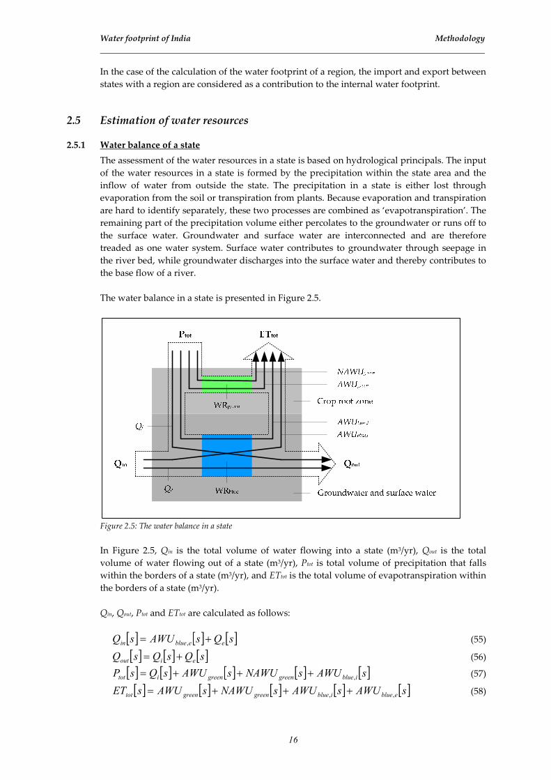
The water balance in a state is presented in Figure 2.5.
Figure 2.5: The water balance in a state
In Figure 2.5, Qin is the total volume of water flowing into a state (m3/yr), Qout is the total
volume of water flowing out of a state (m3/yr), Ptot is total volume of precipitation that falls
within the borders of a state (m3/yr), and ETtot is the total volume of evapotranspiration within
the borders of a state (m3/yr).
Qin, Qout, Ptot and ETtot are calculated as follows:
[ ] [ ] [ ]sQsAWUsQ eebluein += , (55)
[ ] [ ] [ ]sQsQsQ eiout += (56)
[ ] [ ] [ ] [ ] [ ]sAWUsNAWUsAWUsQsP ibluegreengreenitot ,+++= (57)
[ ] [ ] [ ] [ ] [ ]sAWUsAWUsNAWUsAWUsET eblueibluegreengreentot ,, +++= (58)
Water footprint of India Methodology
17
Here, AWUblue,e is the total use of external irrigation water (m3/yr), Qe is the outflow of
external water from the state (m3/yr), Qi is the outflow of internal water from the state (m3/yr),
AWUgreen is the total use of rainwater (m3/yr), NAWUgreen is the total use of rainwater in non
agricultural areas (m3/yr), and AWUblue,i is the total use of internal irrigation water (m3/yr).
As can be seen in Figure 2.5, a distinction is made between green water resources (WRgreen,
m3/yr) and blue water resources (WRblue, m3/yr). The blue water resources can be further
divided into an internal and an external component.
2.5.2 Internal water resources of a state
Green water resources (WRgreen, m3/yr) are by definition internal water resources and are here
defined as the total volume of vapour flows from the surface area in a state under rain fed
conditions.
The WRgreen are calculated as follows:
[ ] [ ] [ ]sNAWUsAWUsWR greengreengreen += (59)
The NAWUgreen are estimated as follows:
[ ] [ ] [ ]( ) [ ]sAsETsPMinsNAWU agricnoneffgreen ∗= 0, (60)
Here, Anonagric is the non agricultural area in a state (ha/yr). It is worth noticing that in this
study, the non agricultural area, from which NAWUgreen is calculated, also represents the
agricultural area that is not taken into account.
The internal blue water resources (WRblue,i, m3/yr) capture the average annual flow in rivers
and the recharge of groundwater generated from endogenous precipitation.
The WRblue,i are calculated as follows:
[ ] [ ] [ ]sWRsPsWR greentotiblue −=, (61)
The total outflow of internal water from a state (Qi, m3/yr) is calculated as follows:
[ ] [ ] [ ]sAWUsWRsQ iblueibluei ,, −= (62)
Here, AWUblue,i is assessed as follows:
[ ] [ ] [ ] [ ]( )sWRsETsWRMinsAWU greentotiblueiblue −= ,,, (63)
In equation 63, the assumption is made that blue water use in a state originates as much as
possible from internal water resources. The calculated AWUblue can now be separated into
AWUblue,i and AWUblue,e. This may lead to an underestimation of Qi and AWUblue,e and to an
overestimation of Qe and AWUblue,i, while Qout remains the same. This also means that AWUblue,e
only becomes larger than zero when Qi becomes zero, which is the case when the Qout is
smaller than Qin.

Water footprint of India Methodology
18
2.5.3 External water resources of a state
The external blue water resources of a state (WRblue,e, m3/yr) are defined as the total average
annual flow in rivers and recharge of groundwater in a state that find their origin in other
states or other countries.
The assumption is made that the volume of groundwater that crosses state borders is
negligible and is therefore omitted in this assessment. Furthermore the assumption is made
that the transport of surface water between across state borders is only in the form of the
larger rivers in India.
The first step in the assessment of interstate river flows is the allocation of the river basin
areas to the involved state areas. The total area of a state in a river basin (As,rb, km2) is
calculated as follows:
[ ] [ ] [ ]sArbArbsA srbrbs I=,, (64)
Here, As is the total area of a state (km2) and Arb is the total area of a river basin (km2).
The part of the outflow of internal water resources of a state that contributes to the discharge
volume of a river basin (Qi,rb, m3/yr) is calculated as follows:
[ ][ ] [ ]
[ ]sA
sQrbsArbsQ
s
irbs
rbi
∗=
,,
,
, (65)
The total outflow of water from a state in a river basin (Qout,rb, m3/yr) is now calculated as
follows:
[ ] [ ] [ ]rbsQrbsQrbsQ rberbirbout ,,, ,,, += (66)
Here, Qe,rb is the part of the outflow of external water resources of a state that contributes to
the discharge volume of river basin rb (m3/yr), which is calculated as follows:
[ ] [ ] [ ]sAWUrbsQrbsQ ebluerbinrbe ,,, ,, −= (67)
In Equation 67, Qin,rb is the inflow of external water resources into a state in a river basin
(m3/yr), which is calculated as follows:
[ ] [ ]∑=
=p
us
rbirbin usrbsQrbsQ1
,, ,,, (68)
Here, us denotes a state upstream of state s, and p is the amount of states upstream of state s in
river basin rb. The states upstream of state s in river basin rb are determined by the flow
direction of the rivers through the states in river basin rb.
The WRblue,e of state s are now calculated as follows:
[ ] [ ]rbsQsWRk
rb
rbineblue ,,, ∑= (69)

Water footprint of India Methodology
19
Here, k is the amount of river basins state s falls in.
The total discharge volume of river basin rb (Qrb, m3/yr) is found as follows:
[ ] [ ]∑=
=n
s
outrb rbsQrbQ1
, (70)
Because of climatic variations within states, this calculation method might lead to an
underestimate or overestimate of the discharge volume of the river basins.
Unlike with the internal blue water resources, the external blue water resources of the states
are interdependent on state scale. This means that the external water use in a state influences
the external water availability downstream. The more states upstream of a state, the less
accurate the calculated volume of external water resources is.
Apart from this, the spatial variations are different for internal and external resources. For the
internal resources the water availability is likely to be more spread over the state area, while
the water availability from the external resources is limited to the area relatively close to the
river flow.
This assessment of water resources differs from other methods of assessing water resources.
First of all, green water resources are taken into account. Second of all, in the assessment of
internal renewable (blue) water resources, the withdrawal of irrigation water is taken into
account.
2.6 Assessment of water scarcity
2.6.1 Water scarcity from production perspective
Traditionally, water scarcity is seen from production perspective (WSprod, (-)) by comparing
water use to the available water resources in a state. This water scarcity is here divided into
green water scarcity (WSprod,green, (-)) and blue water scarcity (WSprod,blue, (-)).
The WSprod, WSprod,green and WSprod,blue are calculated as follows:
[ ][ ] [ ] [ ]
[ ]sWR
sAWUsAWUsAWUsWS
tot
graybluegreen
prod
++= (71)
[ ][ ]
[ ]sWR
sAWUsWS
green
green
greenprod =, (72)
[ ][ ] [ ]
[ ]sWR
sAWUsAWUsWS
blue
grayblue
blueprod
+=, (73)
By definition the water scarcity from production perspective is between 0 and 1. Because of
temporal and spatial dynamics in the water resources, not all water resources can be used and
therefore water scarcity from production perspective will never reach 1. At which volume of

Water footprint of India Methodology
20
water use the water becomes “scarce” is thus determined by the volume of utilizable water
resources in a state.
2.6.2 Water scarcity from consumption perspective
The green and blue water scarcity in a state can also be seen from consumption perspective
(WScons, (-)) by comparing the water footprint to the available water resources in a state. Also
this water scarcity can be divided into green water scarcity (WScons,green, (-)) and blue water
scarcity (WScons,blue, (-)).
The WScons, WScons,green and WScons,blue are calculated as follows:
[ ][ ] [ ] [ ]
[ ]sWR
sWFPsWFPsWFPsWS
tot
graygreenblue
cons
++= (74)
[ ][ ]
[ ]sWR
sWFPsWS
green
green
greencons =, (75)
[ ][ ] [ ]
[ ]sWR
sWFPsWFPsWS
blue
dilutionblue
bluecons
+=, (76)
In contrast to WSprod, the WScons can be more than 1. This is the case when more water is needed
to produce the food for the inhabitants than is available in a state, which is the case in
completely urban states like Delhi.
2.7 Calculation of water saving
2.7.1 Global water saving
Water saving in a state is realised by a net import of a crop. The volume of water it would
have taken to produce the imported amount of crop in the importing state itself is the water
volume that is saved.
The water saving in a state as a result of a net import of a crop (ΔSs, m3/yr) is calculated as
follows:
[ ] [ ] [ ]( ) [ ] [ ]( )( ) [ ]scVWCscEscEscIscIscS insissinsisss ,,,,,, ,,,, ∗+−+=∆ (77)
The global water saving as a result of interstate commodity trade (ΔSg, m3/yr) is calculated as
follows:
[ ] [ ] [ ] [ ]( )eeiiieieg scVWCscVWCsscTsscS ,,,,,, −∗=∆ (78)
It can be seen that global water saving becomes negative (global water loss) when the VWC in
the importing state is lower than the VWC in the exporting state.
The total global water saving as a result of interstate commodity trade is found by summing
up the global water savings of all interstate trade flows of a commodity.

Water footprint of India Methodology
21
The global water saving as a result of interstate trade is divided into a blue, a green and a gray
component. These components are found by calculating with blue, green and gray component
of VWC separately.
2.7.2 Water saving and the theory of comparative advantage
Based on equation 78, water is only globally saved when there is an absolute advantage in
water productivity in the exporting state. This would mean that the export of crops from
states with a natural absolute disadvantage in water productivity will never lead to global
water saving.
However, the economic theory of comparative advantage (Ricardo, 1817) shows how two
states can both gain from crop trade if they specialize in the production of crops for which
they have a comparative advantage and import the crops for which they have a comparative
disadvantage. In the case of water productivity, this means that the absolute water saving that
is realised by focussing on the relative advantage in water productivity is higher than the
absolute water saving that is realised by focussing on the absolute advantage in water
productivity (Wichelns, 2007).
If we consider the states s1 and s2, which both produce the crops c1 and c2, next to the absolute
advantages in water productivity, the relative advantage in water productivity can be
determined.
Equations 79 and 80 present the two possible situations.
[ ][ ]
[ ][ ]22
21
12
11
,
,
,
,
scWP
scWP
scWP
scWP< (79)
[ ][ ]
[ ][ ]22
21
12
11
,
,
,
,
scWP
scWP
scWP
scWP> (80)
In the first situation, state s1 has a comparative advantage in crop c1 and a comparative
disadvantage in crop c2, while state s2 has a comparative advantage in crop c2 and a
comparative disadvantage in crop c1. In the second situation, state s1 has a comparative
advantage in crop c2 and a comparative disadvantage in crop c1, while state s2 has a
comparative advantage in crop c1 and a comparative disadvantage in crop c2.
State s1 should therefore specialize in crop c1 in the first situation and in crop c2 in the second
situation, while state s2 should specialize in crop c2 in the first situation and in crop c1 in the
second situation. These recommended specializations only depend on relative water
productivities.
2.7.3 Relative water saving
Apart from absolute water saving, there is also relative water saving. Relative water saving is
realised by increasing the part of the vapour flow that contributes to the biomass of the crop
(transpiration) at the cost of the non productive part (evaporation), while the total
evapotranspiration remains the same, which means there is no absolute water saving.

Water footprint of India Methodology
22
Figure 2.6 shows that relative water saving can be realised by increasing the agricultural
productivity (Rockström, 2003). This is because with an increase in crop yield, the productive
part of the water productivity of a crop increases.
V
ap
ou
r fl
ow
(m
m)
Figure 2.6: The general relationship between the crop yield and the different components of the vapour flow
(Rockström, 2003)
The productive part of water productivity (WPT, ton/m3) is calculated as follows (Rockström,
2003):
[ ][ ][ ]( )),(1
,,
scbY
ETT
e
scWPscWP
−= (81)
Here, WPET is the total water productivity of a crop (ton/m3) as defined in equation 22, b is an
empirical constant (-), and Y the crop yield (ton/ha). Depending on the climate, b fluctuates
around a value of -0.3 (Rockström, 2003).

23
3. Study scope and data collection
3.1 Study area
India is located in South Asia bordering with Pakistan, China, Nepal, Bhutan, Myanmar and
Bangladesh. In the north, along the border with China, India is situated in the Himalayan
Range. Large rivers like the Indus, the Ganges and the Brahmaputra spring from this
mountainous area. Below the Himalayan Range the Indo-Gangetic Plain is found, which
decreases from the west to the east. In the west, against the border with South Pakistan
(Latitude 25°-28°), the Thar Desert is situated. In the southern peninsular part of India the
Deccan Plateau is found, with coastal hill regions (Western and Eastern Ghats). The southern
part of India is surrounded by the Arabian Sea on the west side and the Bay of Bengal on the
east side. Apart from the Thar Desert these geological features are all visible in the elevation
map of India (Figure 3.1).
Figure 3.1: Elevation map of India (Source: en.wikipedia.org)

Water footprint of India Study scope and data collection
24
On a political scale India is divided into thirty-six administrative divisions; twenty-nine
states, six union territories and the national capital territory Delhi (see Figure 3.2). The six
union territories are Andaman & Nicobar Islands, Chandigarh (also the capital of both Punjab
and Haryana), Dadra & Nagar Haveli, Daman & Diu, Lakshadweep Islands and Pondicherry.
The states and the union territory of Pondicherry have an own local government. The
remaining union territories are directly controlled by the national government, which is
settled in Delhi.
Figure 3.2: Map of the Indian states & Union Territories (CDC, 2007)
Approximately 70 % of the Indian population is currently living in rural areas (FAO, 2006a).
This percentage is decreasing as a result of an increase in urbanisation in the past decades.
In this study the following administrative divisions are excluded; Andaman & Nicobar
Islands, Arunachal Pradesh, Chandigarh, Dadra & Nagar Haveli, Daman & Diu, Goa,
Lakshadweep Islands, Manipur, Meghalaya, Mizoram, Nagaland, Sikkim and Tripura. These
states and union territories are not taken into account, because they either have little area
suitable for agriculture or have a small population (Appendix II). Therefore they are assumed
to have no significant influence on the results of the study. Only in the assessment of the
interstate trade, these areas are included to close the national crop balances. Another reason
for the exclusion of these areas is that the precipitation is not well reported because of the
small amount or even the absence of weather stations.

Water footprint of India Study scope and data collection
25
In November 2000, three states were split into two separate states; Uttaranchal was carved out
of Uttar Pradesh, Jharkhand out of Bihar and Chhattisgarh out of Madhya Pradesh. Since this
happened during the period on which this study is focused, it is worth noticing that data on
the states involved prior November 2000 represent the combined performance of the split up
states, which is separated by their relative individual performance after November 2000.
Finally, the India can also be divided into four larger regions; northern, western, eastern and
southern India. Northern India consists of Jammu & Kashmir, Himachal Pradesh, Punjab,
Haryana, Uttaranchal, Uttar Pradesh and Delhi. Western India consists of Rajasthan, Gujarat,
Madhya Pradesh and Maharashtra. Eastern India consists of Bihar, Jharkhand, West Bengal,
Assam, Orissa and Chhattisgarh. And southern India consists of Karnataka, Andhra Pradesh,
Kerala and Tamil Nadu.
The total area considered in this study is 94% of the total territory of India and covers 98% of
the population (Appendix II).
3.2 Crop coverage
Not all crops that are grown in India can be taken into account in this study. Therefore a
selection of crops is made.
FAO distinguishes 176 primary crops in the FAOSTAT database (FAO, 2006a), of which 80 are
produced in India in the period 1997-2001 (Appendix III). These 80 crops can be summarized
in 12 crop categories. The 12 crop categories and their total water use, production value and
land use are given in Table 3.1.
1 Source: FAO (2006a), 2 Water use = production * Indian average virtual water content (source: Chapagain &
Hoekstra, 2004), 3 Production value = production * producer price (US$ 1997-2001, source: FAO, 2006a).
The water use of a crop is the production volume multiplied with the virtual water content of
the crop (Chapagain & Hoekstra, 2004). The total crop water use in India is 949 billion m3/yr.
Table 3.1. Water use, production value and land use per crop category in the period 1997-2001
Crop categories Production1 Water use2 Production value3 Land use1
106 ton/yr 109 m3/yr % 109 US$/yr % 106 ha/yr %
Cereals 233 581 61 30 39 101 57
Oil crops 37 154 16 10 13 35 20
Pulses 13 58 6 5 6 21 12
Sugar crops 286 46 5 5 7 4 2
Fruits 45 39 4 11 14 4 2
Spices 2 17 2 2 2 3 1
Vegetables 68 16 2 9 11 5 3
Tree nuts 1 10 1 1 1 1 1
Stimulants 1 9 1 1 1 1 0
Starchy roots 30 7 1 3 4 2 1
Vegetable fibres 2 6 1 0 0 1 0
Other 1 6 1 1 1 1 0
Total 719 949 100 77 100 178 100

Water footprint of India Study scope and data collection
26
The value of the annual crop production is captured in the production volume multiplied
with the producer price of a crop (FAO, 2006a). The total production value is 77 billion
US$/yr.
The total net area of arable land in India is approximately 145 million ha (CIA, 2006). The total
gross area harvested (178 million ha/yr) is higher, because arable land can be harvested more
than once in a year.
Since water use is the main focus of this study, a boundary condition is put on the water use
of a crop to determine if a crop may play a significant role in the analysis of this study. The
chosen boundary level on the crop water use is determined at 1% of the total water use. The
assumption that crops may play a significant role when they are above the chosen boundary
level is more or less arbitrary. For this study, the chosen level seemed reasonable and led to a
feasible amount of crops to investigate.
In the crop selection, the production value and land use of a crop are also taken into account.
The excluded crops therefore have a production value that is lower than 5% of the total
production value and a land use that is lower than 2% of the total agricultural area in India.
These parameters are taken into account to avoid the exclusion of crops with a high economic
value or a large land use.
Table 3.2 shows the 16 selected primary crops. This selection represents 80% of the total crop
production, 87% of the total water use, 69% of the total production value and 86% of the total
land use.
Table 3.2. Selected primary crops in the period 1997-2001 ranked by water use
Primary crops in
FAOSTAT
Crop
production1 Water use2 Production value Land use
Name 106 ton/yr 109 m3/yr % 109 US$/yr % 106 ha/yr %
Rice, Paddy 130.9 373.1 39.3 16.5 21.4 44.6 25.0
Wheat 70.6 116.8 12.3 10.4 13.5 26.7 15.0
Seed Cotton 5.7 47.2 5.0 2.9 3.8 8.9 5.0
Sugar Cane 286.0 45.6 4.8 5.1 6.7 4.1 2.3
Millet 10.2 33.2 3.5 1.0 1.3 12.6 7.0
Sorghum 8.0 32.4 3.4 0.9 1.2 10.1 5.7
Soybeans 6.4 26.2 2.8 1.5 1.9 6.3 3.5
Groundnuts in Shell 7.0 23.9 2.5 2.3 3.0 6.8 3.8
Maize 11.8 22.8 2.4 1.3 1.7 6.4 3.6
Beans, Dry 2.6 21.7 2.3 0.8 1.0 6.7 3.8
Coconuts3 9.3 21.1 2.2 0.8 1.1 1.8 1.0
Mangoes3 10.6 16.1 1.7 3.8 4.9 1.4 0.8
Chick-Peas 5.5 14.9 1.6 1.9 2.5 6.8 3.8
Rapeseed 5.4 14.1 1.5 1.7 2.2 6.1 3.4
Pimento, Allspice3 1.0 10.6 1.1 0.8 1.1 0.9 0.5
Pigeon Peas 2.4 9.9 1.0 0.9 1.2 3.5 1.9
Other crops3 145.6 119.2 12.6 24.3 31.5 24.4 13.7
Total 718.9 949.0 100.0 77.0 100.0 178.0 100.0
1 Source: FAO (2006a), 2 Source: Chapagain & Hoekstra (2004) 3 Shaded crops are excluded from study

Water footprint of India Study scope and data collection
27
The primary crop “fresh vegetables not elsewhere specified” is omitted in table 3.2, although
the production value is 5.3% of the national total. The reason for this is that this crop is
already a leftover category within the category vegetables and therefore not suitable for
further investigation, because data on individual crops are necessary to make an equal
comparison between the states possible.
At this point, it can be seen that not all crop categories from table 3.1 are well represented in
the individual crop ranking in table 3.2. Based on these two tables the decision is made that
the selected crops within the crop categories cereals, oil crops, pulses and sugar crops are
further investigated in this study. This means that relatively important crops like mangoes
and pimento are excluded. Furthermore coconut is excluded from this study, because of the
lack of trade data on the processed products of this crop (like coir) and the lack of possible
changes in the location of the crop production. According to this analysis, the selection of
crops now represent 77% of the total crop production, 82% of the total water use, 61% of the
total production value and 84% of the total land use.
Finally, it is worth noticing that although rice is harvested as paddy rice, we only use the
milled rice equivalent, which represents all the processed rice products interpolated to the
equivalent of milled rice. Furthermore, it should be noted that all sugar originates from sugar
cane in India and that the generic name dry beans in this study represents the crops mung
bean, black gram and moth bean.
3.3 Data collection
3.3.1 Climatic parameters
The data on the reference evapotranspiration (ET0) are calculated in CROPWAT (FAO, 2006b).
In this program, the average ET0 is calculated per month with the FAO Penman-Monteith
method for 160 weather stations in India. Climatic data on these weather stations that are
required as the input for this computation are taken from CLIMWAT (FAO, 2006c), which is
the climatic database of CROPWAT. The available weather stations and the accompanying
states are given in Appendix V. The average ET0 in a certain state for a certain month is found
by taking the mean of the ET0 of all the weather stations situated in that state in that month.
The amount of weather stations used per state varies from 1 in Himachal Pradesh and Delhi
to 14 in Uttar Pradesh. In total 9 weather stations are excluded from the calculation of the
average ET0, because they are either situated in non agricultural areas like deserts and
mountains or very clearly cause an uneven distribution of the weather stations over the state
area. The exclusion of these particular stations (Appendix IV) still does not guarantee that the
calculated average ET0 is the “real” average ET0 of the state. In some states there are simple
too few stations to present a reliable value for the entire state.
The Ptot and Peff data for the 160 weather stations are again taken from CLIMWAT (FAO,
2006c) and the average Ptot and Peff per state is again found by taking the mean of the Ptot and
Peff of all the weather stations situated in that state in that month. In the calculation of the
virtual water contents, the same weather stations that are excluded in the calculation of the
average ET0 per month per state are excluded here, because they are either situated in non
agricultural areas like deserts and mountains or very clearly cause an uneven distribution of
the weather stations over the state area. In the calculation of the internal and external blue
water resources this might lead to a small underestimation in the case of the exclusion of
rainy mountainous weather stations and to a small overestimation in the case of the exclusion
of dry desert weather stations.
Water footprint of India Study scope and data collection
28
3.3.2 Crop parameters
Data on the duration of the different growing stages, sowing and harvesting periods and crop
coefficients are taken from Allen et al. (1998), Directorate of Rice Development (2006a) and
Directorate of Pulses Development (2006a).
Because of climatic differences and duration differences of crop varieties, the sowing and
harvesting periods vary per region. To keep this study feasible a maximum of two sets of crop
parameters are created for entire India; one for the wet season (kharif), which is roughly from
June to December, and one for the dry season (rabi), which is roughly from December to
April. For every crop the duration of these seasons is assessed, which is the same for all the
Indian states. The generated parameters of the studied primary crops are presented in
Appendix V.
3.3.3 Irrigated area fraction
The data on the irrigated area fraction (iaf, (-)) are taken from Directorate of Economics and
Statistics (2003, 2004). The primary data are presented as the fraction of the total area of a crop
under irrigation in a state during the agricultural years 1999-2000 and 2000-2001. The average
iaf of these two agricultural years is taken as the total irrigated area fraction (iaftot(-)).
For the crops that are grown in one season, the iaf is equal to iaftot. For the crops that are grown
in two seasons (kharif and rabi), the assumption is made that the iaf during rabi is as high as
possible. The reason for this assumption is that the irrigation water is required the most
during the dry season.
The iaf during rabi and kharif is calculated as follows:
[ ] [ ]( )( )[ ]scA
iafscAscAMiniaf
rabi
tottotrabi
rabi,
,,, ∗= (82)
[ ] [ ][ ]scA
iafscAiafscAiaf
kharif
rabirabitottot
kharif,
,, ∗−∗= (83)
Here, Arabi is the area of crop c in state s during rabi (ha/yr), Akharif is the area of crop c in state s
during kharif (ha/yr) and Atot is the total area of crop c in state s (ha/yr).
In the case of maize in Tamil Nadu, an exception is made for the calculation of the iaf during
kharif and rabi. The reason for this is that in this special case, the irrigation water requirement
as a percentage of the total water requirement is higher during kharif than during rabi.
Therefore the iaf of maize in Tamil Nadu during the wet season is assumed to be as high as
possible.
3.3.4 Dilution water requirement
The data on the use of nitrate in fertilizers are taken from FAO (2005). FAO provides data on
nitrate consumption (kg N/ha) for the most important crops in India in the agricultural year
2003-2004 for irrigated and rain fed areas, in which no distinction is made between the states.
The assumption is made that the values of the year 2003-2004 also apply to the period 1997-
2001.
Since the nitrate use is not given for all studied crops, the following assumptions are made:
• The nitrate use on pearl millet is taken as the nitrate use on finger millet and small millets.
• The nitrate use on pigeon peas is taken as the nitrate use on all pulses and soybean.

Water footprint of India Study scope and data collection
29
The total nitrate use for a crop (Nuse, kg N/ha) is now calculated as follows:
[ ] [ ] [ ] [ ]( ) [ ]scNsciafsciafscNscN rfauseiauseuse ,,1,,, ,, ∗−+∗= (84)
Here, Nuse,ia is the nitrate use on crop c in irrigated areas (kg N/ha), Nuse,rfa is the nitrate use on
crop c in rain fed areas (kg/ha) and iaf is the irrigated area fraction (-).
The total nitrate use by states is taken from Directorate of Economics and Statistics (2003).
These values are used for the comparison of the total gray water use in the different states as
calculated in this study to the total gray water use in the different states as calculated from the
total nitrate use.
The leaching factor of nitrate is in this study determined at 0.10. This value is taken from
Chapagain et al. (2006).
The recommended level of nitrogen (N) in the groundwater is in this study taken to be 10 mg
N/l (EPA, 2006; Chapagain et al., 2006), which corresponds with a nitrate (NO3¯) level of 44
mg/l (Agrawal, 1999).
There are twelve states in India where nitrate levels are measured in the groundwater above
the recommended level (Ministry of Water Resources, 2006a). The highest nitrate levels are
found in Haryana and Punjab (Agrawal, 1999).
3.3.5 Product and value fractions of crops
The product fractions of the crops for India are taken from FAO (2006a, 2006d) and are based
on data from the period 1992-1996. The assumption is made that these values are still accurate
for our study period. The value fractions are taken from Chapagain & Hoekstra (2004). The
product and value fractions of the studied crops used in this study are presented in Appendix
VI.
3.3.6 Population
The urban and rural population of the states are taken from Census of India (2006) and FAO
(2006a). Census of India gives detailed data for the year 2001 for every state and FAO gives
the total urban and rural population for the years 1997-2001. The average population during
the study period is found by combining the total number from FAO with the state distribution
from Census of India. A map of the variation in the population density over the country and
the total rural and urban population per state are presented in Appendix II.
Data on the average income per state in the period 1997-2001 is taken from Chandigarh
Administration (2006).
3.3.7 National crop balance
In the national crop balance, the domestic supply (production, import, export, stock change)
and the domestic utilization (animal feed, seed, manufacturing, waste, uses and food) of a
crop are determined for the study period 1997-2001 (Appendix VII). In this study, the national
balance of a crop is the average of the five annual crop balances, which are taken from the five
annual food balance sheets of India (FAO, 2006a). In the cases when the primary crop is
processed before consumption, the national balance is given for the primary crop and the
processed crop. These annual crop balances are chosen as a base in this study, because no
other balance includes other utilizations than human consumption.

Water footprint of India Study scope and data collection
30
In the national crop balance of sugar cane, the production, seed, feed, manufacture and food
volumes for sugar cane for the years 1998 and 1999 have been adjusted to the production and
utilization volumes of sugar cane as presented by the statistical database of the Indian
Institute of Sugarcane Research (IISR, 2006). This is done because IISR are likely to present
more reliable data.
The national crop balance of the crop category pulses is only given for dry beans, dry peas
and other pulses (FAO, 2006a). Since dry peas is not taken into account in this study and the
utilizations of dry beans and other pulses are of the same percentage, the national balance is
only assessed for pulses as a whole.
Since there is no national balance for cotton lint, the assumption is made that all produced
cotton lint that is not exported (FAO, 2006a), is used for local human consumption or
exported to other states.
3.3.8 Crop area, production and yield
The production data of cereals, oil crops and pulses are taken from Directorate of Economics
and Statistics (2003, 2004), Directorate of Rice Development (2006b), Directorate of Wheat
Development (2006), Directorate of Pulses Development (2006b) and FAORAP (2006). The
production data of sugarcane are taken from the statistical database of the Indian Institute of
Sugarcane Research (IISR, 2006). The production data of oil crops for the year 1997 is not
available on state level and is therefore estimated on the total national production during 1997
and the relative state production volumes during the other years of the study period.
The state production volumes are divided over the two main crop seasons in India:
• kharif (wet monsoon season), which is approximately from June to November
• rabi (dry winter season), which is approximately from November to April
Besides these two main seasons, there are also crops grown during the summer season (also
known as the pre-kharif season), which is approximately from April to September, and thus
overlaps the other two seasons. But since the crop production during this period is very low,
this season is not taken into account in this study. The crop production during this season is
either added to the crop production in the kharif season or to the crop production in the rabi
season.
The primary production data are presented in agricultural years, which are from July to June,
while the data in the crop balances are presented in calendar years, which are from January to
December (see Figure 3.3). Therefore, the production data from 1996-1997 to 2000-2001 are
used for the rabi crops and the production data from 1997-1998 to 2001-2002 are used for the
kharif crops. If a crop is grown in both seasons, the season with the largest crop production
determines if the crop is here considered as a rabi crop or a kharif crop. This means that, for
example, in the case of milled rice, kharif is considered as the main season, which means that
the rabi production of calendar year 2002 is used and the rabi production of calendar year
1997 is excluded. In this step the following crops are considered as rabi crops; wheat, sugar
cane, rapeseed and chickpeas. All other crops are here considered as kharif crops.

Water footprint of India Study scope and data collection
31
Figure 3.3: The overlap of calendar years and agricultural years
3.3.9 Crop consumption
The data on the consumption of crops in the different states are all taken from reports of
NSSO. This organisation carries out socio-economic surveys throughout India on a regular
basis. This means that the consumption of most commodities is estimated at least every five
years. NSSO provides the state consumption per capita in rural and urban areas.
For the crop category cereals, the consumption data for the years 1997-2001 are taken from the
NSSO (1998, 1999, 2001a, 2002, 2003). For the crop categories oil crops and sugar crops, the
consumption data for the year 1999-2000 are taken from NSSO (2001b). For the crop category
pulses, the consumption data for the year 1999-2000 are taken from NSSO (2001a). And for
cotton lint, the consumption data for the year 2000-2001 are taken from NSSO (2002).
In the consumption data of oil crops, sugar crops and pulses some unrealistically high values
are found for three north eastern states (Arunachal Pradesh, Manipur and Mizoram). For
these states, the consumption data for year 1993-1994 are taken from NSSO (1997).
The total computed annual consumption per state (Cs,comp, ton/yr) is generated as follows:
[ ] [ ] [ ] urbanurbancapruralruralcapcomps PopscCPopscCscC ∗+∗= ,,, ,,, (85)
Here, Ccap,rural is consumption of a crop per capita in the rural area of a state (ton/cap/yr), Poprural
is the rural population is a state (cap), Ccap,urban is consumption of a crop per capita in the urban
area of a state (ton/cap/yr) and Popurban is the urban population in a state (cap).
Next, the computed consumption volume of a state is interpolated to the consumption
volume as given in the state crop balance (Cs, ton/yr), which is done to keep the national crop
balance closed.
The Cs is now calculated as follows:
[ ]
[ ][ ]
[ ]∑=
∗
=n
s
comps
t
comps
s
pf
scC
cCpf
scC
scC
1
,
,
,
,
, (86)
Here, Ct is the consumption in the national crop balance (ton/yr) and pf the product fraction of
the edible equivalent of crop c (-).
In general, the total computed crop consumption is a little lower than consumption as given
in the national crop balance. But similarity between these two national crop consumption

Water footprint of India Study scope and data collection
32
volumes can be expected, because FAO regularly uses specific information on consumption
trends from household surveys for benchmarking their estimates for subsequent years.
According to FAO, the difference between the two numbers reflects “waste occurring between
the retail level and the kitchen and losses of edible food and nutrients in the household, e.g.,
during storage, in preparation and cooking (which affect vitamins and minerals to a greater
extent than calories, protein and fat), as plate-waste, or as quantities fed to domestic animals
and pets, or that thrown away”.
Only in the case of chickpeas, non centrifugal and raw sugar, soybean and other edible oils,
the computed consumption is significantly lower than the consumption as given in the
national crop balance. The reason for this can be the exclusion of intermediate crop
consumption in the NSSO method (NSSO, 2005). Intermediate consumption is here
interpreted as the part of the crop that is used up in the process of further production (for
example in factories or restaurants). The fact that there is a considerable volume of
intermediate crop consumption in the case of crops involved is realistic. In the case of
chickpeas, 60% is processed into a flour known as besan (Price et al., 2003), which is often
mixed with flour from cereals. In the case of raw cane sugar, a large amount ends up in
sweets, which are very popular in India, or other products. In the case of soybean and other
edible oils, the soybean cake is processed into flour, which can again be mixed with flour from
cereals, and a large part of the oil ends up in a mix of soybean oil and palm oil, which is
known as vanaspati (Dohlman et al., 2003).
In the special case of pigeon peas, the computed consumption is higher than the consumption
in the national balance. This overestimation seems to indicate an error in the assessment of
either FAO (2006a) or NSSO (2001a).
Finally, it should be noted that the consumption data of cotton lint is presented as the average
monthly expenditure on clothing per capita. Here, the assumption is made that the share of
cotton lint in clothing is equal for all states. Since the consumption values are interpolated to
the total value in the national balance, the unit of the consumption data does not form a
problem.
3.3.10 Interstate trade
For the crops that are processed before consumption, the surplus and interstate trade are
calculated in the edible equivalent. The reason for this is that the processed crop may have a
by-product with a certain value that might be traded differently. An example of this is
soybean which is processed into soybean oil and soybean cake. In these cases, the export,
animal feed and primary crop consumption in the national balance of the primary crop are
first transformed to the processed equivalent by the product fraction and then added to the
crop utilizations in the national balance of the processed crop.
In the case of pulses, the surplus of pulses is only calculated for pulses as a whole and the
assumption is made that the interstate trade consists of chickpeas only. The reason for this is
that, apart from the individual crop balances that are lacking, the computed consumption
values of the individual pulses are too dodgy. The assumption is made that summing up the
individual pulse consumption before the interpolation to the national balance eventually
gives a better indication of total pulse consumption in a state than summing up after
interpolating to the national balance. This assumption is based on the principle that
individual pulses are exchangeable, which means that locally produced pulses are consumed
before imported pulses. The interstate trade of pulses is caused by the interstate export of
pulses from Madhya Pradesh, Maharashtra and Rajasthan. Based on the reported
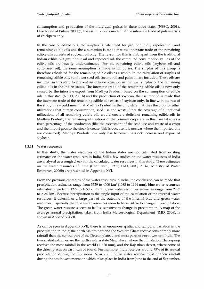
Water footprint of India Study scope and data collection
33
consumption and production of the individual pulses in these three states (NSSO, 2001a,
Directorate of Pulses, 2006b)), the assumption is made that the interstate trade of pulses exists
of chickpeas only.
In the case of edible oils, the surplus is calculated for groundnut oil, rapeseed oil and
remaining edible oils and the assumption is made that the interstate trade of the remaining
edible oils consists of soybean oil only. The reason for this is that, apart from the traditional
Indian edible oils groundnut oil and rapeseed oil, the computed consumption values of the
edible oils are heavily underestimated. For the remaining edible oils (soybean oil and
cottonseed oil), the same assumption is made as for pulses. The surplus of this group is
therefore calculated for the remaining edible oils as a whole. In the calculation of surplus of
remaining edible oils, sunflower seed oil, coconut oil and palm oil are included. These oils are
included in this step, to prevent an oblique situation in the final surplus of the remaining
edible oils in the Indian states. The interstate trade of the remaining edible oils is now only
caused by the interstate export from Madhya Pradesh. Based on the consumption of edible
oils in this state (NSSO, 2001b) and the production of soybean, the assumption is made that
the interstate trade of the remaining edible oils exists of soybean only. In line with the rest of
the study this would mean that Madhya Pradesh is the only state that uses the crop for other
utilizations that human consumption, seed use and waste. Since the coverage of all national
utilizations of all remaining edible oils would create a deficit of remaining edible oils in
Madhya Pradesh, the remaining utilizations of the primary crops are in this case taken as a
fixed percentage of the production (like the assessment of the seed use and waste of a crop)
and the import goes to the stock increase (this is because it is unclear where the imported oils
are consumed). Madhya Pradesh now only has to cover the stock increase and export of
soybean.
3.3.11 Water resources
In this study, the water resources of the Indian states are not calculated from existing
estimates on the water resources in India. Still a few studies on the water resources of India
are analysed as a rough check for the calculated water resources in this study. These estimates
on the water resources of India (Chaturvedi, 1985; FAO, 2003, 2006e; Ministry of Water
Resources, 2006b) are presented in Appendix XVI.
From the previous estimates of the water resources in India, the conclusion can be made that
precipitation estimates range from 3559 to 4000 km3 (1083 to 1194 mm), blue water resources
estimates range from 1272 to 1650 km3 and green water resources estimates range from 2287
to 2350 km3. Because precipitation is the single input of the calculation of the internal water
resources, it determines a large part of the outcome of the internal blue and green water
resources. Especially the blue water resources seem to be sensitive to change in precipitation.
The green water resources seem to be less sensitive to change in precipitation. A map of the
average annual precipitation, taken from India Meteorological Department (IMD, 2006), is
shown in Appendix XVII.
As can be seen in Appendix XVII, there is an enormous spatial and temporal variation in the
precipitation in India; the north eastern part and the Western Ghats receive considerably more
rainfall than the central part of the Deccan plateau and most parts of north western India. The
two spatial extremes are the north eastern state Meghalaya, where the hill station Cherrapunji
receives the most rainfall in the world (11420 mm), and the Rajasthan desert, where some of
the driest places on earth can be found. Furthermore, India receives around 75% of its annual
precipitation during the monsoons. Nearly all Indian states receive most of their rainfall
during the south west monsoon which takes place in India from June to the end of September.

Water footprint of India Study scope and data collection
34
Only Tamil Nadu receives most of its rainfall during the north east monsoon which takes
place in India from October to December.
Since precipitation is of large importance for the outcome of the estimates on water resources,
rainfall data are taken from IITM (2006), which collected rainfall data for India from the year
1871 and onwards. In these data four Himalayan states are excluded; Jammu & Kashmir,
Himachal Pradesh, Uttaranchal and Arunachal Pradesh. These data lead to an average annual
precipitation of 1088 mm.
In the calculation of the external blue water resources, the data on state areas situated in river
basins and the direction of rivers through the Indian states (Appendix XIX) are taken from
Ministry of Water Resources (2006c).
The total annual inflow of water from other countries (China, Nepal and Bhutan) is taken to
be 636 km3 (FAO, 2006e). This estimate is for a large part based on one rough number (347
km3) of the Chinese government, which represents the inflow from China to Jammu &
Kashmir (Indus river basin) and Arunachal Pradesh (Brahmaputra river basin). Based on data
of the weather stations in Jammu & Kashmir, it seems that the eastern part of this state, where
the Indus enters the country, receives very little rainfall. It is worth noticing that the highest
Himalayan Range which is in India situated in the states of Himachal Pradesh and
Uttaranchal seems to act as a precipitation barrier. This conclusion is based on data from
weather stations in the involved states and the annual rainfall map of India. The assumption
is made that the precipitation in the far western part of Tibet, where the Indus springs from, is
of the same magnitude as in the eastern part of Jammu & Kashmir. This assumption lead to
the estimate that 20 km3 of water annually enters India through the Indus river basin (10 km3
in the Indus and 10 km3 in the Satluj tributary). This estimate means that a volume 327 km3 of
water flows from China to India through the Brahmaputra basin. The inflow from Nepal and
Bhutan is estimated at 210 km3 and 90 km3 (FAO, 2006e). The inflow from Nepal enters India
in the states Uttar Pradesh and Bihar and is thereby part of the Ganges river basin. FAO
estimates that the distribution is 80 km3 to Uttar Pradesh and 130 km3 to Bihar. The inflow
from Bhutan contributes entirely to the Brahmaputra basin though the states West Bengal and
Assam. In this study the assumption is made that the distribution is 15 km3 to West Bengal
and 75 km3 to Assam, which is based on the percentage of the total area of Bhutan that
contribute to the two Indian states.

35
4. Virtual water content of crops
4.1 Virtual water content of the primary crops
The blue, green, gray and total virtual water content of the primary crops is tabulated by state
in Appendix VIII. The virtual water content of crops that are grown during kharif (wet
season) as well as rabi (dry season), is presented for kharif, rabi and the total of both seasons,
which is the average of both seasons weighted by the seasonal production in a state.
In general, the virtual water content of the crops is relatively lower in the northern and
southern states and relatively higher in the western and eastern states. This variation in
virtual water contents is largely determined by the difference in crop yield. This difference is
mainly caused by the difference in development of the agricultural areas, which can be
expressed in the form of a high or low fraction of irrigated area and a high or low fertilizer
use. Another reason for a variation in the virtual water content of a crop is the difference in
climate. In general, the influence of climate on the magnitude of the virtual water content is
not very high. On one hand, a higher evapotranspiration rate leads to a higher crop water
requirement and therefore to a higher crop water use, but on the other hand, a higher
evapotranspiration rate leads to a higher biomass of the crop, which leads to a higher yield.
However, with a lower crop yield, the non productive part of the evapotranspiration rate (the
part that does not contribute to the biomass of the crop) is relatively higher and therefore the
influence of the climate on the virtual water content is relatively higher.
The blue, green and gray component of the total water use is given by crop in Figure 4.1.
0
50
100
150
200
250
300
350
Milled
rice
Wheat Coarse
cereals
Sugar
cane
Pulses Oil crops Seed
cotton
Wa
ter
use
(b
illi
on
m3
/yr)
Gray
Green
Blue
Figure 4.1: The blue, green and gray volume of water used in India for crop production in the period 1997-2001.

Water footprint of India Virtual water contents of crops
36
The total volume of water used in India for the production of the studied primary crops is 792
billion m3/yr. The total blue water use is 219 billion m3/yr, the total green water use 479 billion
m3/yr and the total gray water use billion 95 m3/yr.
Figure 4.1 shows that the production of milled rice is responsible for a water use of 348 billion
m3/yr, which is 44% of the total water use, and that the production of wheat uses a water
volume of 100 billion m3/yr, which is 13% of the total water use. Furthermore Figure 4.1
shows that the water use in case of milled rice consists mainly (67%) of green water and that
the water use in case of wheat consists mainly (58%) of blue water.
According to Directorate of Economics and Statistics (2003), the average nitrate use in India
during the study period is 11.2 billion kg N/yr. Applying the leaching factor of 10% and a
recommended level of 10 mg N/l, this translates in a total gray water use of 112 billion m3/yr
for the dilution of the total nitrate consumption in the Indian agriculture. This means that 85%
of the total gray water use is represented in this study. Since this gray water use is based on
the average nitrate use for crops in whole India, the calculated gray water use is compared to
the total nitrate consumption per state (Directorate of Economics and Statistics, 2003). This
comparison shows that the gray water use in Andhra Pradesh, Karnataka and Punjab is
underestimated in this study and that the gray water use is Madhya Pradesh, Chhattisgarh,
Orissa and Rajasthan is overestimated (Appendix IX).
In this study, the crops grown in the dry season (rabi) in non irrigated areas receive too little
water during the growth period, which results in an underestimation of the virtual water
content of a crop (Appendix VIII). The first reason for this underestimation of crop water use
is the fact that a crop might be grown in a part of a state which receives more precipitation
than the state average precipitation, which is used in this study. An example of this is the
growth of soybean in Rajasthan under rain fed conditions, which takes place in the relatively
wet south eastern part of the state. Another reason might be an incorrect assessment of the
growth periods of the crops in the different states, which are in this study taken to be the
same for all states. A third reason can be the fact that there might still be green water available
in the soil after the monsoon, which is not taken into account in this study.
4.2 Virtual water content of milled rice
Because milled rice is the crop with the largest contribution to the water use in India, the
virtual water content of milled rice is described here with more detail.
The virtual water content of milled rice varies from 2914 m3/ton in Punjab to 8142 m3/ton in
Madhya Pradesh, with a national average of 4073 m3/ton. The wide range in the virtual water
content of milled rice in India is mainly caused by differences in crop yield, which has a large
correlation with the fraction of the crop area under irrigation (Appendix X).
The yield of milled rice grown under rain fed conditions is considerably lower than the yield
of milled rice grown under irrigated conditions, which is caused by a higher potential yield of
the variety that is grown under irrigation, which requires a high level of irrigation and a high
fertilizer use (Directorate of Rice Development, 2006c).
The variation of the virtual water content of milled rice over the Indian states is shown in
Figure 4.2.
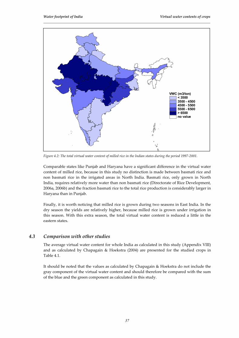
Water footprint of India Virtual water contents of crops
37
VWC (m3/ton)< 35003500 - 45004500 - 55005500 - 6500> 6500 no value
Figure 4.2: The total virtual water content of milled rice in the Indian states during the period 1997-2001.
Comparable states like Punjab and Haryana have a significant difference in the virtual water
content of milled rice, because in this study no distinction is made between basmati rice and
non basmati rice in the irrigated areas in North India. Basmati rice, only grown in North
India, requires relatively more water than non basmati rice (Directorate of Rice Development,
2006a, 2006b) and the fraction basmati rice to the total rice production is considerably larger in
Haryana than in Punjab.
Finally, it is worth noticing that milled rice is grown during two seasons in East India. In the
dry season the yields are relatively higher, because milled rice is grown under irrigation in
this season. With this extra season, the total virtual water content is reduced a little in the
eastern states.
4.3 Comparison with other studies
The average virtual water content for whole India as calculated in this study (Appendix VIII)
and as calculated by Chapagain & Hoekstra (2004) are presented for the studied crops in
Table 4.1.
It should be noted that the values as calculated by Chapagain & Hoekstra do not include the
gray component of the virtual water content and should therefore be compared with the sum
of the blue and the green component as calculated in this study.
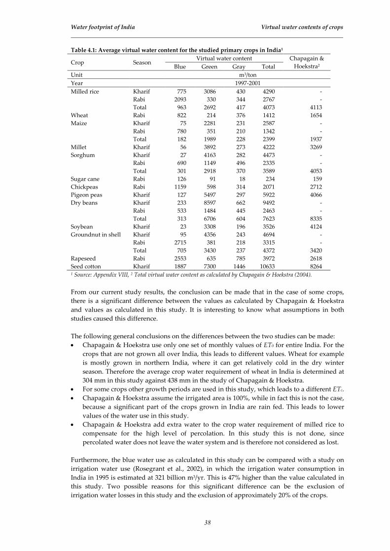
Water footprint of India Virtual water contents of crops
38
Table 4.1: Average virtual water content for the studied primary crops in India1
Crop Season Virtual water content Chapagain &
Hoekstra2 Blue Green Gray Total
Unit m3/ton
Year 1997-2001
Milled rice Kharif 775 3086 430 4290 -
Rabi 2093 330 344 2767 -
Total 963 2692 417 4073 4113
Wheat Rabi 822 214 376 1412 1654
Maize Kharif 75 2281 231 2587 -
Rabi 780 351 210 1342 -
Total 182 1989 228 2399 1937
Millet Kharif 56 3892 273 4222 3269
Sorghum Kharif 27 4163 282 4473 -
Rabi 690 1149 496 2335 -
Total 301 2918 370 3589 4053
Sugar cane Rabi 126 91 18 234 159
Chickpeas Rabi 1159 598 314 2071 2712
Pigeon peas Kharif 127 5497 297 5922 4066
Dry beans Kharif 233 8597 662 9492 -
Rabi 533 1484 445 2463 -
Total 313 6706 604 7623 8335
Soybean Kharif 23 3308 196 3526 4124
Groundnut in shell Kharif 95 4356 243 4694 -
Rabi 2715 381 218 3315 -
Total 705 3430 237 4372 3420
Rapeseed Rabi 2553 635 785 3972 2618
Seed cotton Kharif 1887 7300 1446 10633 8264 1 Source: Appendix VIII, 2 Total virtual water content as calculated by Chapagain & Hoekstra (2004).
From our current study results, the conclusion can be made that in the case of some crops,
there is a significant difference between the values as calculated by Chapagain & Hoekstra
and values as calculated in this study. It is interesting to know what assumptions in both
studies caused this difference.
The following general conclusions on the differences between the two studies can be made:
• Chapagain & Hoekstra use only one set of monthly values of ET0 for entire India. For the
crops that are not grown all over India, this leads to different values. Wheat for example
is mostly grown in northern India, where it can get relatively cold in the dry winter
season. Therefore the average crop water requirement of wheat in India is determined at
304 mm in this study against 438 mm in the study of Chapagain & Hoekstra.
• For some crops other growth periods are used in this study, which leads to a different ETc.
• Chapagain & Hoekstra assume the irrigated area is 100%, while in fact this is not the case,
because a significant part of the crops grown in India are rain fed. This leads to lower
values of the water use in this study.
• Chapagain & Hoekstra add extra water to the crop water requirement of milled rice to
compensate for the high level of percolation. In this study this is not done, since
percolated water does not leave the water system and is therefore not considered as lost.
Furthermore, the blue water use as calculated in this study can be compared with a study on
irrigation water use (Rosegrant et al., 2002), in which the irrigation water consumption in
India in 1995 is estimated at 321 billion m3/yr. This is 47% higher than the value calculated in
this study. Two possible reasons for this significant difference can be the exclusion of
irrigation water losses in this study and the exclusion of approximately 20% of the crops.

39
5. Interstate and interregional virtual water flows
5.1 Interstate and international product trade
The production, consumption and surplus of crops are given for the Indian states in
Appendix XI. Furthermore, the distribution of the international and interstate trade of the
Indian states is described in Appendix XII.
In general, a high production of a crop in a state means a high consumption of that crop in
that state. For example, millets and sorghum grow well in dry areas and it no coincidence that
the production and consumption of millets and sorghum is high in the dry western part of
India. An exception to this rule is the production of rice in the northern states, where the
production is high and the consumption relatively low.
In Table 5.1, the total production, interstate trade and net import of the crops are given. It can
be seen that milled rice, wheat and sugar cause the largest interstate trade in India.
Table 5.1: National production, interstate trade and net national import of the studied crops
Crop National production Interstate trade Net international import
Unit Million ton/yr
Year 1997-2001
Milled rice 87.1 10.5 - 2.6
Wheat 70.6 13.3 0.1
Maize 11.7 0.3 0
Millet 10.1 1.7 0
Sorghum 7.9 0.9 0
- Total coarse cereals - 29.7 2.9 0
Raw sugar 30.1 8.7 0.1
Pulses1 13.4 2.2 0.8
Groundnut oil 1.6 0.3 0
Rapeseed oil 1.7 0.9 0.1
Remaining edible oils2,3 2.0 0.1 3.5
- Total edible oils - 5.3 1.3 3.6
Soybean cake4 5.0 - - 2.5
Cotton lint 1.9 0.3 0.9 1 Interstate trade in pulses consists of chickpeas only. 2 Remaining edible oils are soybean oil, sunflower seed oil,
cottonseed oil and coconut oil. 3 Interstate trade in remaining edible oils consists of soybean oil only. 4 Trade in
soybean cake consists of international trade only.
The crops with largest trade flows are milled rice, wheat and sugar. The main reason behind
the magnitude of these flows is the Public Distribution System that exists for these crops. This
system is controlled by the Indian government, which procures the crops mainly in northern
states Punjab, Haryana, Uttar Pradesh. This is because these states have a developed trade
infrastructure.
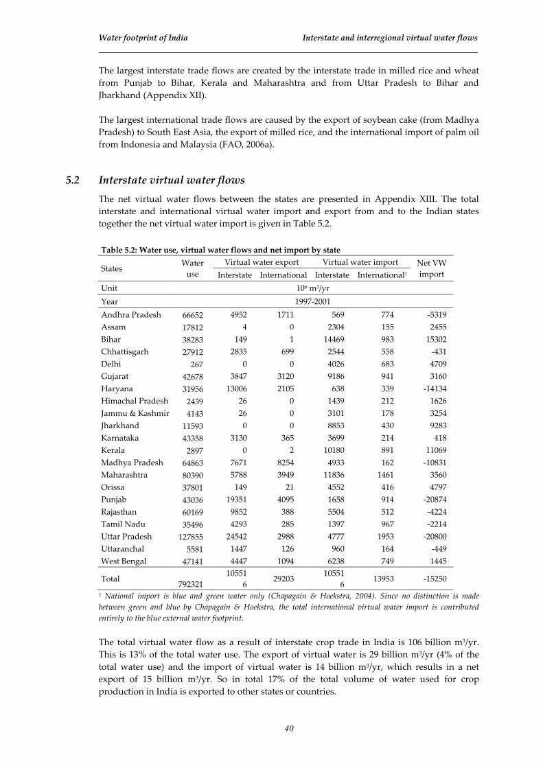
Water footprint of India Interstate and interregional virtual water flows
40
The largest interstate trade flows are created by the interstate trade in milled rice and wheat
from Punjab to Bihar, Kerala and Maharashtra and from Uttar Pradesh to Bihar and
Jharkhand (Appendix XII).
The largest international trade flows are caused by the export of soybean cake (from Madhya
Pradesh) to South East Asia, the export of milled rice, and the international import of palm oil
from Indonesia and Malaysia (FAO, 2006a).
5.2 Interstate virtual water flows
The net virtual water flows between the states are presented in Appendix XIII. The total
interstate and international virtual water import and export from and to the Indian states
together the net virtual water import is given in Table 5.2.
Table 5.2: Water use, virtual water flows and net import by state
States Water
use
Virtual water export Virtual water import Net VW
import Interstate International Interstate International1
Unit 106 m3/yr
Year 1997-2001
Andhra Pradesh 66652 4952 1711 569 774 -5319
Assam 17812 4 0 2304 155 2455
Bihar 38283 149 1 14469 983 15302
Chhattisgarh 27912 2835 699 2544 558 -431
Delhi 267 0 0 4026 683 4709
Gujarat 42678 3847 3120 9186 941 3160
Haryana 31956 13006 2105 638 339 -14134
Himachal Pradesh 2439 26 0 1439 212 1626
Jammu & Kashmir 4143 26 0 3101 178 3254
Jharkhand 11593 0 0 8853 430 9283
Karnataka 43358 3130 365 3699 214 418
Kerala 2897 0 2 10180 891 11069
Madhya Pradesh 64863 7671 8254 4933 162 -10831
Maharashtra 80390 5788 3949 11836 1461 3560
Orissa 37801 149 21 4552 416 4797
Punjab 43036 19351 4095 1658 914 -20874
Rajasthan 60169 9852 388 5504 512 -4224
Tamil Nadu 35496 4293 285 1397 967 -2214
Uttar Pradesh 127855 24542 2988 4777 1953 -20800
Uttaranchal 5581 1447 126 960 164 -449
West Bengal 47141 4447 1094 6238 749 1445
Total 792321
10551
6 29203
10551
6 13953 -15250
1 National import is blue and green water only (Chapagain & Hoekstra, 2004). Since no distinction is made
between green and blue by Chapagain & Hoekstra, the total international virtual water import is contributed
entirely to the blue external water footprint.
The total virtual water flow as a result of interstate crop trade in India is 106 billion m3/yr.
This is 13% of the total water use. The export of virtual water is 29 billion m3/yr (4% of the
total water use) and the import of virtual water is 14 billion m3/yr, which results in a net
export of 15 billion m3/yr. So in total 17% of the total volume of water used for crop
production in India is exported to other states or countries.

Water footprint of India Interstate and interregional virtual water flows
41
In Table 5.2, it can be seen that the northern states Punjab, Haryana and Uttar Pradesh have a
very high virtual water export and that the states Bihar, Jharkhand and Kerala have a very
high virtual water import. The state with the largest net international export of virtual water
is Madhya Pradesh. This is mainly caused by the international export of soybean cake from
this state.
In Figure 5.1, the virtual water balances of the states are presented in the form of the net
virtual water import. Furthermore, the net interstate virtual water flows larger than 2 billion
m3/yr are shown to indicate the largest interstate virtual water flows.
Net VW import
(billion m3/yr)
< - 10
-10 - -5-5 - -1
-1 - 00 - 1
1 - 55 - 10> 10no value
Figure 5.1: The net virtual water import of the Indian states and the largest net interstate virtual water flows (> 2
billion m3/yr) during the period 1997-2001.
In Figure 5.1, it can be seen that the states with the highest net export of virtual water are
directly connected with the states with the highest net import of virtual water by the largest
net interstate virtual water flows between these states. The most striking large virtual water
flows are the long distance flows from Punjab and Haryana to Bihar, Gujarat, Maharashtra
and Kerala. This shows that Punjab and Haryana produce food for states all over India.
Furthermore, it is worth noticing that the states with a net virtual water export as well as the
states with a net virtual water import are more or less grouped together. This may indicate a
natural advantage or disadvantage through the geology, climate, population or consumption
pattern of a region.

Water footprint of India Interstate and interregional virtual water flows
42
The contribution of the crops to the blue, green, gray and total interstate virtual water flow
and net national virtual water import are presented in Table 5.3.
Table 5.3: Interstate virtual water flows and net national virtual water import by crop
Crop Interstate virtual water flows Net national
VW import Blue Green Gray Total
Unit Million m3/yr
Year 1997-2001
Milled rice 12790 20246 3829 36865 -9032
Wheat 6495 2686 3754 12936 670
Coarse cereals 313 10132 801 11245 -104
Raw sugar 9238 6895 1320 17453 100
Pulses1 3109 1217 724 5050 589
Edible oils2 7708 5107 2159 14974 8259
Soybean cake3 - - - - -8164
Cotton lint 1276 4762 953 6992 -7568
Total 40931 51044 13541 105516 -15250 1 Interstate virtual water flow of pulses consists of chickpeas only. 2 Interstate trade of remaining edible oils consists
of soybean oil only. 3 Trade of soybean cake consists of international trade only.
Table 5.3 shows that 35% of the interstate virtual water flow is due to interstate trade of milled
rice, 17% due to interstate trade of raw sugar and 14% due to interstate trade of edible oils.
5.3 Interregional virtual water flows
The virtual water flows between the four large regions are calculated to show the rough
direction of the virtual flows within India (Figure 5.2).
Figure 5.2: The net virtual water flows between the four regions of India in 109 m3/yr during the period 1997-2001.
Water footprint of India Interstate and interregional virtual water flows
43
Figure 5.2 shows that the largest interregional virtual water flow is from North India to East
India. This virtual water flow has a volume of 22 billion m3/yr and consists for 54% of rice, for
21% of raw sugar and for 18% of wheat. Furthermore, this total water volume of 22 billion
m3/yr consists for 38% of blue water, 48% of green water and for 14% of gray water. The
interregional virtual water flow from North to East India originates for 66% from Uttar
Pradesh, 19% from Punjab and 13% from Haryana and is destined for 52% for Bihar, 29% for
Jharkhand and 14% for West Bengal.
Table 5.2 and Figure 5.2 show a total net international export of virtual water of 15 billion
m3/yr. This shows a relatively good resemblance with the study of Chapagain & Hoekstra
(2004), in which the net international export of virtual water is determined at 18 billion m3/yr.

44
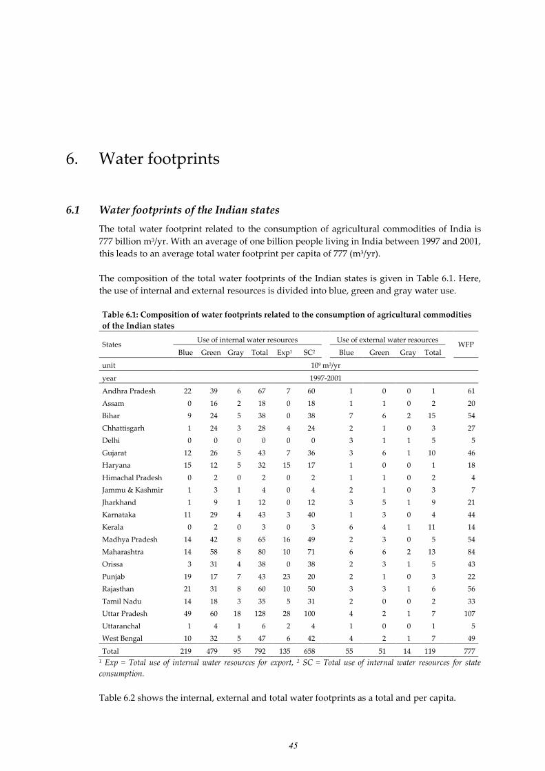
45
6. Water footprints
6.1 Water footprints of the Indian states
The total water footprint related to the consumption of agricultural commodities of India is
777 billion m3/yr. With an average of one billion people living in India between 1997 and 2001,
this leads to an average total water footprint per capita of 777 (m3/yr).
The composition of the total water footprints of the Indian states is given in Table 6.1. Here,
the use of internal and external resources is divided into blue, green and gray water use.
Table 6.1: Composition of water footprints related to the consumption of agricultural commodities
of the Indian states
States Use of internal water resources Use of external water resources
WFP Blue Green Gray Total Exp1 SC2 Blue Green Gray Total
unit 109 m3/yr
year 1997-2001
Andhra Pradesh 22 39 6 67 7 60 1 0 0 1 61
Assam 0 16 2 18 0 18 1 1 0 2 20
Bihar 9 24 5 38 0 38 7 6 2 15 54
Chhattisgarh 1 24 3 28 4 24 2 1 0 3 27
Delhi 0 0 0 0 0 0 3 1 1 5 5
Gujarat 12 26 5 43 7 36 3 6 1 10 46
Haryana 15 12 5 32 15 17 1 0 0 1 18
Himachal Pradesh 0 2 0 2 0 2 1 1 0 2 4
Jammu & Kashmir 1 3 1 4 0 4 2 1 0 3 7
Jharkhand 1 9 1 12 0 12 3 5 1 9 21
Karnataka 11 29 4 43 3 40 1 3 0 4 44
Kerala 0 2 0 3 0 3 6 4 1 11 14
Madhya Pradesh 14 42 8 65 16 49 2 3 0 5 54
Maharashtra 14 58 8 80 10 71 6 6 2 13 84
Orissa 3 31 4 38 0 38 2 3 1 5 43
Punjab 19 17 7 43 23 20 2 1 0 3 22
Rajasthan 21 31 8 60 10 50 3 3 1 6 56
Tamil Nadu 14 18 3 35 5 31 2 0 0 2 33
Uttar Pradesh 49 60 18 128 28 100 4 2 1 7 107
Uttaranchal 1 4 1 6 2 4 1 0 0 1 5
West Bengal 10 32 5 47 6 42 4 2 1 7 49
Total 219 479 95 792 135 658 55 51 14 119 777 1 Exp = Total use of internal water resources for export, 2 SC = Total use of internal water resources for state
consumption.
Table 6.2 shows the internal, external and total water footprints as a total and per capita.
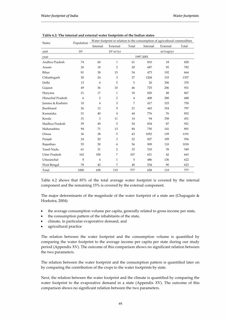
Water footprint of India Water footprints
46
Table 6.2: The internal and external water footprints of the Indian states
States Population Water footprint in relation to the consumption of agricultural commodities
Internal External Total Internal External Total
unit 106 109 m3/yr m3/cap/yr
year 1997-2001
Andhra Pradesh 74 60 1 61 810 18 828
Assam 26 18 2 20 687 95 782
Bihar 81 38 15 54 473 192 664
Chhattisgarh 20 24 3 27 1204 153 1357
Delhi 13 0 5 5 20 350 370
Gujarat 49 36 10 46 725 206 931
Haryana 21 17 1 18 820 48 867
Himachal Pradesh 6 2 2 4 408 280 688
Jammu & Kashmir 10 4 3 7 417 333 750
Jharkhand 26 12 9 21 443 354 797
Karnataka 51 40 4 44 776 76 852
Kerala 31 3 11 14 94 358 451
Madhya Pradesh 59 49 5 54 834 87 921
Maharashtra 94 71 13 84 750 141 891
Orissa 36 38 5 43 1052 139 1191
Punjab 24 20 3 22 827 109 936
Rajasthan 55 50 6 56 909 110 1018
Tamil Nadu 61 31 2 33 510 39 549
Uttar Pradesh 162 100 7 107 621 42 663
Uttaranchal 8 4 1 5 486 136 622
West Bengal 78 42 7 49 534 90 623
Total 1000 658 119 777 658 119 777
Table 6.2 shows that 85% of the total average water footprint is covered by the internal
component and the remaining 15% is covered by the external component.
The major determinants of the magnitude of the water footprint of a state are (Chapagain &
Hoekstra, 2004):
• the average consumption volume per capita, generally related to gross income per state,
• the consumption pattern of the inhabitants of the state,
• climate, in particular evaporative demand, and
• agricultural practice
The relation between the water footprint and the consumption volume is quantified by
comparing the water footprint to the average income per capita per state during our study
period (Appendix XV). The outcome of this comparison shows no significant relation between
the two parameters.
The relation between the water footprint and the consumption pattern is quantified later on
by comparing the contribution of the crops to the water footprints by state.
Next, the relation between the water footprint and the climate is quantified by comparing the
water footprint to the evaporative demand in a state (Appendix XV). The outcome of this
comparison shows no significant relation between the two parameters.

Water footprint of India Water footprints
47
The relation between the water footprint and agricultural practice is already assessed in
Chapter 4, where the reasons for low water productivity in a state are addressed. A low water
productivity leads to a relatively high internal water footprint of a state.
The variation in water footprints per capita between the Indian states is shown in Figure 6.1.
WFP (m3/cap/yr)< 700700 - 800800 - 900900 - 1000> 1000no value
Figure 6.1: Water footprints of the Indian states per capita
The three states with the highest water footprint per capita are Chhattisgarh and Orissa in
eastern India and Rajasthan in Western India. These states have a high water footprint,
because the water productivity is low (Chapter 4) and the virtual water import is low
(Chapter 5). In these states the water productivity is low, because of inefficient agricultural
practice.
The lowest water footprints are found in the southern states Kerala and Tamil Nadu and in
the national territory of Delhi. One reason for the low water footprints of Kerala and Tamil
Nadu is the exclusion of coconut, which is part of the staple food in these states, in this study.
Especially in the case of Kerala, this is main reason for the low internal water footprint. Kerala
produces approximately half of the national coconut production (Directorate of Economics
and Statistics, 2003, 2004). According to Chapagain & Hoekstra (2004) this would mean a
water volume of around 10 billion m3/yr used for the production of coconut in Kerala.
Assuming that most of the coconut is consumed within Kerala, this would mean a significant
increase of the internal water footprint, which is determined at 3 billion m3/yr in this study.
Furthermore, it should be noted that the water footprints of Kerala and Tamil Nadu are also
relatively low as a result other local staple food, like the starchy root cassava, which has a low
virtual water content. The reason for this is that a relatively large part of starchy roots is
edible.
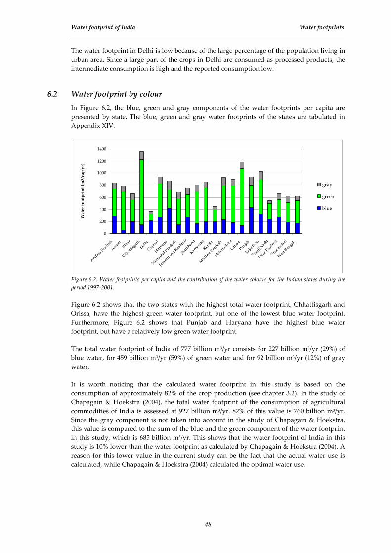
Water footprint of India Water footprints
48
The water footprint in Delhi is low because of the large percentage of the population living in
urban area. Since a large part of the crops in Delhi are consumed as processed products, the
intermediate consumption is high and the reported consumption low.
6.2 Water footprint by colour
In Figure 6.2, the blue, green and gray components of the water footprints per capita are
presented by state. The blue, green and gray water footprints of the states are tabulated in
Appendix XIV.
0
200
400
600
800
1000
1200
1400
Andhra
Pra
desh
Ass
amBih
ar
Chhat
tisgarh
Del
hi
Guja
rat
Hary
ana
Him
achal
Pra
desh
Jam
mu
and K
ashm
ir
Jhark
hand
Kar
nata
ka
Ker
ala
Madhya
Pra
desh
Mahara
shtr
a
Oris
sa
Punjab
Rajast
han
Tamil
Nadu
Utta
r Pra
desh
Utta
ranc
hal
Wes
t Ben
gal
Wat
er f
oo
tpri
nt
(m3/
cap
/yr)
gray
green
blue
Figure 6.2: Water footprints per capita and the contribution of the water colours for the Indian states during the
period 1997-2001.
Figure 6.2 shows that the two states with the highest total water footprint, Chhattisgarh and
Orissa, have the highest green water footprint, but one of the lowest blue water footprint.
Furthermore, Figure 6.2 shows that Punjab and Haryana have the highest blue water
footprint, but have a relatively low green water footprint.
The total water footprint of India of 777 billion m3/yr consists for 227 billion m3/yr (29%) of
blue water, for 459 billion m3/yr (59%) of green water and for 92 billion m3/yr (12%) of gray
water.
It is worth noticing that the calculated water footprint in this study is based on the
consumption of approximately 82% of the crop production (see chapter 3.2). In the study of
Chapagain & Hoekstra (2004), the total water footprint of the consumption of agricultural
commodities of India is assessed at 927 billion m3/yr. 82% of this value is 760 billion m3/yr.
Since the gray component is not taken into account in the study of Chapagain & Hoekstra,
this value is compared to the sum of the blue and the green component of the water footprint
in this study, which is 685 billion m3/yr. This shows that the water footprint of India in this
study is 10% lower than the water footprint as calculated by Chapagain & Hoekstra (2004). A
reason for this lower value in the current study can be the fact that the actual water use is
calculated, while Chapagain & Hoekstra (2004) calculated the optimal water use.

Water footprint of India Water footprints
49
6.3 Water footprint by crop
Besides the distinction between the blue, green and gray water footprint, the total water
footprint can be divided into the water footprint of the individual crops.
The contribution of the studied crops to the water footprints of the Indian states are presented
in Figure 6.3.
0
200
400
600
800
1000
1200
1400
And
hra P
rades
h
Ass
amBih
ar
Chh
attis
garh
Del
hi
Guja
rat
Hary
ana
Him
achal
Pra
desh
Jam
mu a
nd Kash
mir
Jhark
hand
Karn
ataka
Ker
ala
Mad
hya P
rades
h
Mah
arash
tra
Oris
sa
Punja
b
Rajas
than
Tamil
Nadu
Utta
r Pra
desh
Utta
ranch
al
Wes
t Ben
gal
Wa
ter
foo
tpri
nt
(m3
/ca
p/y
r)
cotton lint
edible oils
pulses
sugar
coarse cereals
wheat
rice
Figure 6.3: Water footprints per capita and the contribution of the different crops for the Indian states during the
period 1997-2001.
Figure 6.3 shows that there is a relation between the water footprint and consumption pattern.
The water footprint is significantly influenced by the fact that the staple food in a state
consists of rice or wheat, or the fact that there is a high or low level of oil and sugar
consumption. The magnitude of the water footprint of a state is determined by the average
virtual water content of the crops that are consumed in that state.
6.4 Water footprint by region
The internal, external and total water footprint of the four regions of India is given as a total
and per capita in Table 6.3. In the calculation of the water footprint of a region, the interstate
virtual water flows within a region are considered as part of the internal water footprint.
Table 6.3: Water footprints of the consumption of agricultural commodities of the Indian regions
States Total state region footprint Water footprint per capita
Internal External Total Internal External Total
unit 109 m3/yr m3/cap/yr
year 1997-2001
North 154 15 169 632 62 694
East 175 41 215 655 153 808
West 211 29 240 820 113 933
South 137 16 153 629 75 704
Total 658 119 777 658 119 777

Water footprint of India Water footprints
50
The region with the highest water footprint is West India. This is mainly because of the
combination of a low water productivity, a low development of agricultural practice and a
high evapotranspiration rate in this region.
6.5 Water scarcity
The total water resources of the Indian states are given in Appendix XVIII as a state total and
by capita. The interstate water flows are given by river basin in Appendix XIX.
Figure 6.4 shows the current total water scarcity per capita from consumption perspective,
which is the total water footprint divided by the total water resources.
WFP / WR< 0.100.10 - 0.200.20 - 0.30> 0.30no value
Figure 6.4: Total water scarcity from consumption perspective in the Indian states during the period 1997-2001.
Figure 6.4 shows that the total water scarcity from a consumption perspective is the highest is
Rajasthan and Haryana. Furthermore the water scarcity is relatively high is Punjab, Uttar
Pradesh, Gujarat, Maharashtra and Tamil Nadu. Since the water productivity is relatively
high in most of these areas, these states can be considered as naturally scarce.
The lowest water scarcity from consumption perspective can be found in the mountainous
areas and in Bihar and West Bengal. The utilizable percentage of the water resources is
relatively low in these states. In the mountainous areas this is due to a lack of storage and
agricultural area and in Bihar and West Bengal, most of the water resources consist of external
water in the form of the discharge of Ganges. The discharge in the Ganges is the highest
during the monsoon season, in which often flooding occurs in Bihar and West Bengal and the
additional water is not usable.
The green, blue and total water scarcity from a production and consumption perspective is
given by state in Table 6.4.
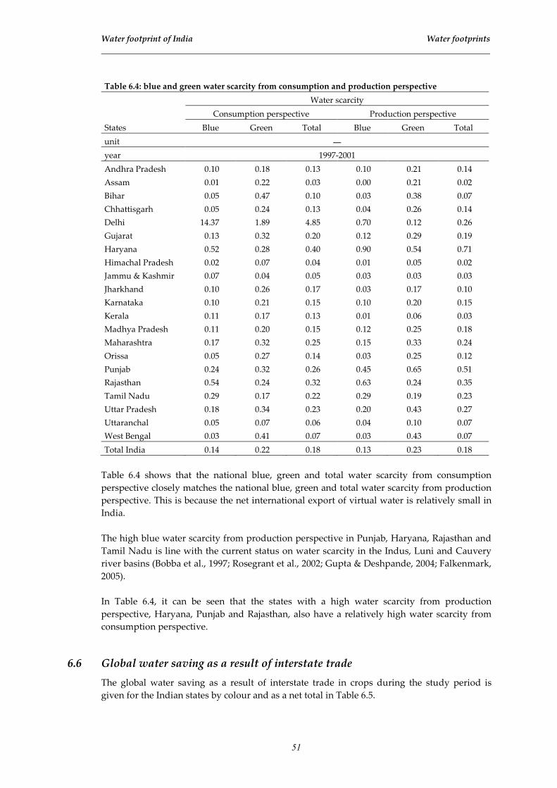
Water footprint of India Water footprints
51
Table 6.4: blue and green water scarcity from consumption and production perspective
States
Water scarcity
Consumption perspective Production perspective
Blue Green Total Blue Green Total
unit ―
year 1997-2001
Andhra Pradesh 0.10 0.18 0.13 0.10 0.21 0.14
Assam 0.01 0.22 0.03 0.00 0.21 0.02
Bihar 0.05 0.47 0.10 0.03 0.38 0.07
Chhattisgarh 0.05 0.24 0.13 0.04 0.26 0.14
Delhi 14.37 1.89 4.85 0.70 0.12 0.26
Gujarat 0.13 0.32 0.20 0.12 0.29 0.19
Haryana 0.52 0.28 0.40 0.90 0.54 0.71
Himachal Pradesh 0.02 0.07 0.04 0.01 0.05 0.02
Jammu & Kashmir 0.07 0.04 0.05 0.03 0.03 0.03
Jharkhand 0.10 0.26 0.17 0.03 0.17 0.10
Karnataka 0.10 0.21 0.15 0.10 0.20 0.15
Kerala 0.11 0.17 0.13 0.01 0.06 0.03
Madhya Pradesh 0.11 0.20 0.15 0.12 0.25 0.18
Maharashtra 0.17 0.32 0.25 0.15 0.33 0.24
Orissa 0.05 0.27 0.14 0.03 0.25 0.12
Punjab 0.24 0.32 0.26 0.45 0.65 0.51
Rajasthan 0.54 0.24 0.32 0.63 0.24 0.35
Tamil Nadu 0.29 0.17 0.22 0.29 0.19 0.23
Uttar Pradesh 0.18 0.34 0.23 0.20 0.43 0.27
Uttaranchal 0.05 0.07 0.06 0.04 0.10 0.07
West Bengal 0.03 0.41 0.07 0.03 0.43 0.07
Total India 0.14 0.22 0.18 0.13 0.23 0.18
Table 6.4 shows that the national blue, green and total water scarcity from consumption
perspective closely matches the national blue, green and total water scarcity from production
perspective. This is because the net international export of virtual water is relatively small in
India.
The high blue water scarcity from production perspective in Punjab, Haryana, Rajasthan and
Tamil Nadu is line with the current status on water scarcity in the Indus, Luni and Cauvery
river basins (Bobba et al., 1997; Rosegrant et al., 2002; Gupta & Deshpande, 2004; Falkenmark,
2005).
In Table 6.4, it can be seen that the states with a high water scarcity from production
perspective, Haryana, Punjab and Rajasthan, also have a relatively high water scarcity from
consumption perspective.
6.6 Global water saving as a result of interstate trade
The global water saving as a result of interstate trade in crops during the study period is
given for the Indian states by colour and as a net total in Table 6.5.
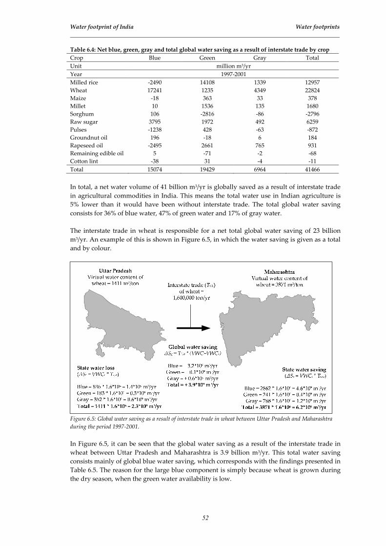
Water footprint of India Water footprints
52
Table 6.4: Net blue, green, gray and total global water saving as a result of interstate trade by crop
Crop Blue Green Gray Total
Unit million m3/yr
Year 1997-2001
Milled rice -2490 14108 1339 12957
Wheat 17241 1235 4349 22824
Maize -18 363 33 378
Millet 10 1536 135 1680
Sorghum 106 -2816 -86 -2796
Raw sugar 3795 1972 492 6259
Pulses -1238 428 -63 -872
Groundnut oil 196 -18 6 184
Rapeseed oil -2495 2661 765 931
Remaining edible oil 5 -71 -2 -68
Cotton lint -38 31 -4 -11
Total 15074 19429 6964 41466
In total, a net water volume of 41 billion m3/yr is globally saved as a result of interstate trade
in agricultural commodities in India. This means the total water use in Indian agriculture is
5% lower than it would have been without interstate trade. The total global water saving
consists for 36% of blue water, 47% of green water and 17% of gray water.
The interstate trade in wheat is responsible for a net total global water saving of 23 billion
m3/yr. An example of this is shown in Figure 6.5, in which the water saving is given as a total
and by colour.
Figure 6.5: Global water saving as a result of interstate trade in wheat between Uttar Pradesh and Maharashtra
during the period 1997-2001.
In Figure 6.5, it can be seen that the global water saving as a result of the interstate trade in
wheat between Uttar Pradesh and Maharashtra is 3.9 billion m3/yr. This total water saving
consists mainly of global blue water saving, which corresponds with the findings presented in
Table 6.5. The reason for the large blue component is simply because wheat is grown during
the dry season, when the green water availability is low.

Water footprint of India Water footprints
53
The interstate trade in milled rice is responsible for a net total global water saving of 13 billion
m3/yr. An example of this is shown in Figure 6.6, in which the global water saving is given as
a total and by colour.
Figure 6.6: Global water saving as a result of interstate trade in milled rice between Uttar Pradesh and Bihar
during the period 1997-2001.
Figure 6.6 shows that the global water saving as a result of the interstate trade in milled rice
from Uttar Pradesh to Bihar is 1.1 billion m3/yr. Figure 6.6 and Table 6.5 show that interstate
trade in milled rice leads to global green and gray water saving, but to global blue water loss.
The interstate trade in raw cane sugar is responsible for a net total global water saving of 6
billion m3/yr. In Figure 6.7 shows an example of water saving by colour and as a total, in
which the interstate trade in raw cane sugar leads to global water loss.
<ttar PradeshVirtual water content of raw
sugar R 2467 m3/ton
West BengalVirtual water content of raw
sugar R 1543 m3/ton
State water loss(ΔSs = VWCe * Tt,is)
Blue R 1286 S 0.7S106 R 0.9S109 m3/yrGreen R 981 S 0.7S106 R 0.7S109 m3/yrGray R 200 S 0.7S106 R 0.1S109 m3/yr
Total = 2467 > 0.7>106 = 1.7>109 m3/yr
State water saving(ΔSs = VWCi * Tt,is)
Blue R 219 S 0.7S106 R 0.2S109 m3/yrGreen R 1171 S 0.7S106 R 0.8S109 m3/yr
Gray R 152 S 0.7S106 R 0.1S109 m3/yrTotal = 1543 > 0.7>106 = 1.1>109 m3/yr
Global water savingΔSg = Tt,is * (VWCi-VWCe)
Blue R - 0.7S109 m3/yrGreen R T 0.1S109 m3/yrGray R - 0.0S109 m3/yrTotal = - 0.6>109 m3/yr
Interstate trade (Tt,is) of raw sugar R700,000 ton/yr
Figure 6.7: Global water saving as a result of interstate trade in raw cane sugar between Uttar Pradesh and West
Bengal during the period 1997-2001.

Water footprint of India Water footprints
54
In Figure 6.7, it can be seen that the interstate trade in raw cane sugar between Uttar Pradesh
and West Bengal leads to a global water loss of 0.6 billion m3/yr. Figure 6.7 and Table 6.4 show
that interstate trade in raw cane sugar leads to global blue water saving, but to a green and
gray global blue water loss.
In the case of sorghum and pulses, the interstate trade leads to considerable net global water
loss. The interstate trade in sorghum is responsible for a net total global water loss of 3 billion
m3/yr. An example of this is shown in Figure 6.8, in which the global water saving is given as
a total and by colour.
Figure 6.8: Global water loss as a result of interstate trade in sorghum between Tamil Nadu and Karnataka during
the period 1997-2001.
Figure 6.8 shows that the interstate trade in sorghum between Tamil Nadu and Karnataka
leads to a global water loss of 0.2 billion m3/yr. Figure 6.8 and Table 6.4 show that interstate
trade in sorghum leads to global green and gray water loss, but to global blue water saving.
6.7 Water saving as a result of comparative advantage in water productivity
The interstate trade in crops that leads to a global water loss can still be justified from a water
management perspective with the theory of comparative advantage.
The state of Rajasthan has an absolute disadvantage in the water productivity of most of its
crops. This is because of a dry hot climate in combination with a low development of
agricultural practice. When only absolute advantages in water productivity are observed, the
conclusion would be that the export of most crops leads to global water loss and that water
will be saved when this export of virtual water from Rajasthan is stopped.
The theory of comparative advantage shows that the elimination of export of virtual water
from Rajasthan does not necessarily lead to water saving. This is because the theory of
comparative advantage focuses on relative advantages in water productivity instead of

Water footprint of India Water footprints
55
absolute advantages in water productivity. The logic behind this theory is that when a state
has an absolute disadvantage in water productivity of all crops, the maximum global benefit
from the state water resources is created when these water resources are used to produce the
crop, of which the water productivity has the least absolute disadvantage.
In the period 1997-2001, Rajasthan exported 0.10 million ton/yr of chickpeas to Punjab and
0.12 million ton/yr of rapeseed oil to Uttar Pradesh and imported 0.40 million ton/yr of wheat
from Punjab and 0.50 million ton/yr of raw sugar from Uttar Pradesh.
The global water saving as a result of interstate trade in chickpeas and wheat between
Rajasthan and Punjab is shown in Figure 6.9.
Figure 6.9: Global water savings as a result of interstate trade in chickpeas and wheat between Rajasthan and
Punjab the period 1997-2001.
Figure 6.9 shows that the interstate trade in wheat from Punjab to Rajasthan leads to global
water saving and that the interstate trade in chickpeas from Rajasthan to Punjab leads to
global water loss.
The global water saving as a result of interstate trade in rapeseed oil and raw sugar between
Rajasthan and Uttar Pradesh is shown in Figure 6.10.

Water footprint of India Water footprints
56
Figure 6.10: Global water savings as a result of interstate trade in rapeseed oil and raw sugar between Rajasthan
and Uttar Pradesh during the period 1997-2001.
Figure 6.10 shows that the interstate trade in raw sugar from Uttar Pradesh to Rajasthan leads
to global water saving and that the interstate trade in rapeseed oil from Rajasthan to Uttar
Pradesh leads to global water loss.
In Table 6.5 the opportunity cost of chickpeas, wheat, rapeseed oil and raw sugar are given for
the states Rajasthan, Punjab and Uttar Pradesh. These opportunity costs are found by
comparing the water productivity of the competitive crops in the states involved. In this case,
all the crops that are involved are grown in the dry season and are therefore considered as
competitive.
Table 6.5: Opportunity costs of chickpeas, wheat, rapeseed oil and raw sugar in the states Rajasthan,
Punjab and <ttar Pradesh during the period 1997-2001
Crops Opportunity costs
Rajasthan Punjab Uttar Pradesh
Unit -
1.00 ton of chickpeas 0.73 ton of wheat 0.42 ton of wheat -
1.00 ton of wheat 1.37 ton of chickpeas 2.36 ton of chickpeas -
1.00 ton of rapeseed oil 0.31 ton of raw sugar - 0.23 ton of raw sugar
1.00 ton of raw sugar 3.25 ton of rapeseed oil - 4.37 ton of rapeseed oil
Table 6.5 shows that the opportunity cost of chickpeas is higher in Rajasthan than in Punjab,
that the opportunity cost of wheat is higher in Punjab than in Rajasthan, that the opportunity
cost of rapeseed oil is higher Rajasthan than in Uttar Pradesh and that the opportunity cost of
raw sugar is higher in Uttar Pradesh than in Rajasthan.
Table 6.6 now shows the change in the production of the crops involved when the virtual
water flows from Rajasthan are eliminated and the total water use in the importing and
exporting states remains equal. In Table 6.6, the assumption is made that Punjab and Uttar
Pradesh will produce the previously imported amount of chickpeas and rapeseed oil
themselves and will reduce the production and export of wheat and raw sugar to keep the
water use equal. Rajasthan will consequently produce the amount of wheat and raw sugar

Water footprint of India Water footprints
57
that is no longer imported from Punjab and Uttar Pradesh and will reduce the production of
chickpeas and rapeseed oil to keep the water use equal.
Table 6.6: The change in crop production with the elimination of the export of chickpeas from
Rajasthan to Punjab and the export of rapeseed oil from Rajasthan to <ttar Pradesh in the period
1997-2001 when the total water use in the states remains equal
Rajasthan Punjab Uttar Pradesh Total
Unit Million ton/yr
Chickpeas - 0.17 T 0.10 - - 0.07
Wheat T 0.24 - 0.24 - 0
Rapeseed oil - 0.16 - T 0.12 - 0.04
Raw sugar T 0.52 - - 0.52 0
Table 6.6 shows that the elimination of export of chickpeas and rapeseed oil from Rajasthan to
Punjab and Uttar Pradesh, leads to a decrease in crop production, while the water use
remains equal. This means that although this export of chickpeas and rapeseed oil leads to
global water loss, the water loss would be even larger when these export flows are eliminated.
Another state that has an absolute disadvantage in the water productivity of most its crops is
Madhya Pradesh. This is mainly because of the low development of agricultural practice. The
theory of comparative advantage again shows that the export of some crops can still be
justified from water management perspective in Madhya Pradesh.
In the period 1997-2001, Madhya Pradesh exported 0.12 million ton/yr of soybean oil and 0.40
million ton/yr of wheat to the rest of India and imported 1.30 million ton/yr of raw sugar and
0.40 million ton/yr of milled rice from the rest of India.
The global water saving as a result of the interstate export of soybean oil and wheat from
Madhya Pradesh and the interstate import of raw sugar and milled rice into Madhya Pradesh
is shown in Figure 6.10.
Figure 6.11: Global water saving as a result of interstate trade in soybean oil, wheat, raw sugar and milled rice
between Madhya Pradesh and the rest of India during the period 1997-2001.

Water footprint of India Water footprints
58
Figure 6.11 shows that the interstate export of soybean oil and wheat from Madhya Pradesh
leads to global water loss and that the interstate import of raw sugar and milled rice into
Madhya Pradesh leads to global water saving.
Table 6.7 shows the opportunity cost of soybean oil, milled rice, wheat and raw sugar for
Madhya Pradesh and for the rest of India. These opportunity costs are found by comparing
the water productivity of the competitive crops in the states involved. In this case, soybean oil
and milled rice are seen as competitive because they are both grown in the wet season and
wheat and raw sugar are seen as competitive because they are both grown in the dry season.
Table 6.7: Opportunity costs of soybean oil, milled rice, wheat and raw sugar in Madhya Pradesh
and whole India during the period 1997-2001
Crops Opportunity costs
Madhya Pradesh India
Unit -
1.00 ton of soybean oil 0.88 ton of milled rice 1.64 ton of milled rice
1.00 ton of milled rice 1.13 ton of soybean oil 0.61 ton of soybean oil
1.00 ton of wheat 0.49 ton of raw sugar 0.63 ton of raw sugar
1.00 ton of raw sugar 2.04 ton of wheat 1.58 ton of wheat
Table 6.7 shows that the opportunity cost of soybean oil and wheat is higher in Madhya
Pradesh than in the rest of India and that the opportunity cost of milled rice and raw sugar is
higher in the rest of India than in Madhya Pradesh.
Table 6.8 now shows the change in production with the elimination of the virtual water flows
from Madhya Pradesh when the total water use in the importing and exporting states remains
equal. In Table 6.8, the assumption is made that the rest of India will produce the previously
imported amount of soybean oil and wheat itself and will reduce the production and export
of milled rice and raw sugar to keep the water use equal. Madhya Pradesh will consequently
produce the amount of milled rice and raw sugar that is no longer imported and will reduce
the production of soybean oil and wheat to keep the water use equal.
Table 6.8: The change in crop production with the elimination of the interstate export of soybean oil
and wheat from Madhya Pradesh in the period 1997-2001 when the total water use in the states
remains equal
Madhya Pradesh India Total
Unit Million ton/yr
Soybean oil - 0.22 T 0.12 - 0.10
Milled rice T 0.20 - 0.20 0
Wheat - 0.52 T 0.40 - 0.12
Raw sugar T 0.25 - 0.25 0
Table 6.8 shows that the elimination of the export of soybean oil and wheat from Madhya
Pradesh to the rest of India, leads to a decrease in crop production, while the water use
remains equal. This means that although this export of soybean oil and wheat leads to global
water loss, the water loss would be even larger when these export flows are eliminated.
59
7. Food security: River interlinking versus increasing
water productivity
7.1 Strategies for Indian water management
The Indian population will be approximately 1.6 billion people in the year 2050 (United
Nations, 2006). Furthermore, the average wealth in India is also growing rapidly. This will
lead to an absolute increase in the food demand.
From the perspective of water resources management, in which food production equals water
use, there are in general three alternative strategies to meet the increasing food demand:
• Water self sufficiency on state level
• Water self sufficiency on national level
• National virtual water import
Here, water self sufficiency means that a state or nation only uses its current internal and
external water resources for food self sufficiency.
The first alternative is a situation where all Indian states are water self sufficient. This would
mean that the consumption pattern should be shifted to those crops that yield the most with
the water resources in the particular state.
The second alternative is the situation where India is nationally water self sufficient and thus
food self sufficient. This is more or less the current situation in which states are importing
virtual water from other states.
The third alternative is a situation in which water self sufficiency is no longer obtained and
virtual water is imported from other countries. Falkenmark (1997, 2005) claims that, in the
case of India, virtual water import will be necessary in the near future and that food self
sufficiency as a goal will have to be given up. However, this alternative is currently not
considered as an option by the Indian government.
If India wants to remain food self sufficient with its rapidly growing population, given that
there is a minimum of water use needed to produce the daily diet of the Indian people, water
scarcity must be reduced.
At the moment, the Indian government is considering the project of the Interlinking of Rivers
(ILR). ILR aims to reduce the water scarcity in water deficit regions by increasing the local
water resources with the import of water through the newly constructed connections of rivers.

Water footprint of India Food security
60
7.2 River interlinking project
The idea of inter basin water transfer have been introduced by Rao (1973), who proposed a
link between Ganges river basin and Cauvery river basin. Currently, the project is on the
verge of being implemented. This shows that water scarcity is considered as a serious issue by
the Indian government at the moment.
The ILR project is divided in a Himalayan and a peninsular component. In total, 174 billion m3
of water is aimed to be transported through the proposed links; 33 billion m3 for the
redistribution of water in the Himalayan component and 141 billion m3 for the redistribution
of water in the peninsular component (Gupta & Deshpande, 2004). The reason for the
relatively low water transport in the Himalayan component is the fact that the Brahmaputra
and Brahmani-Baitani river basins, which have a large water surplus, flow at a lower
elevation than the Ganges river basin. In this study only the Himalayan component of the ILR
project is considered. The reason for this is the fact that the outcome of the interstate and
interregional virtual water flows in Chapter 5 offers a better base for comparing the aimed
water transport to the virtual water flows.
In Figure 7.1, the proposed links for the Himalayan component of the ILR are presented. It
can be seen that all links are meant to transport water from East India to North India. At state
level, the links divert water flows to increase the water resources in Haryana, Rajasthan and
Uttar Pradesh at the cost of the water resources in Bihar, Jharkhand and West Bengal. In total,
33 billion m3/yr of water is meant to be transported through the entire Himalayan component.
The aimed water transport by link is however still unclear.
Figure 7.1: Proposed links of inter basin water transfer in the Himalayan component (NWDA, 2006)
The absence of detailed data on the proposed links contributes to the uncertainty in the
project. Since many negative side effects can be expected, many scientists are sceptic about the
ILR project.
What is striking is the fact that the total water transport through the proposed links in Figure
7.1 has a direction which closely matches the opposite of the direction of the largest
interregional virtual water flow, which is from North India to East India (Chapter 5.3).

Water footprint of India Food security
61
Since the real and virtual flows are opposite to each other, the question rises if it is possible to
eliminate both flows. This is done by taking away the dependency of food import of East
India. Since water is not the limiting factor to the crop production in East India, an increase in
water productivity in that region can lead to an increase in crop production. The question is
whether this increase in water productivity in East India is possible.
7.3 Increasing water productivity
7.3.1 Potential yield
An increase of the water productivity of a crop starts with the increase of the yield of a crop.
This is possible when a significant gap exists between the current and potential yield of crop.
Potential yield is defined here as the maximum yield that can be generated for a certain crop
in a certain state when all needs for an optimal crop growth are supplied. The current yield of
a crop depends on many factors; climate (the occurrence of drought or flooding and the
amount of sun hours), irrigated or rain fed area, amount of fertilizer use, use of high yielding
varieties, water salinity, access to energy (diesel pumps or electricity), tribal or non tribal area
(Phansalkar & Verma, 2005) and soil type. We assume that the potential crop yield only
depends on the climate.
To demonstrate the result of a possible increase in yield, the example of milled rice in Bihar,
Punjab and Uttar Pradesh is used here. This example is used because Bihar is largest importer
of virtual water in East India, Punjab and Uttar Pradesh are the largest exporters of virtual
water in North India, and milled rice is the crop with the largest contribution to the virtual
water flow from North to East India. In this example only milled rice grown during kharif is
taken into account, because this offers a better comparison between the states.
During the study period, the yield of milled rice in Bihar during kharif is 1476 kg/ha. This
results in an annual production of 5.1 million ton of milled rice. This is not enough to meet the
annual consumption in Bihar of 7.1 million ton of milled rice. The deficit is mainly imported
from the northern states Uttar Pradesh and Punjab. The yield of milled rice in Punjab in the
study period is 3403 kg/ha and in Uttar Pradesh 2031 kg/ha.
The difference in yield between the three states is mainly caused by the fraction irrigated area.
In Punjab this fraction is 0.992, while in Uttar Pradesh this is 0.657 and in Bihar 0.393. In the
irrigated areas, a rice variety is grown that requires relatively more fertilizer and a reliable
supply of water (through irrigation), but has a considerable higher yield than the rice variety
grown in the rain fed areas. This rice variety was introduced during the green revolution,
which started in Asia in the late sixties of the previous century.
Based on climatic factors, Uttar Pradesh and Bihar have a slightly lower potential yield than
Punjab. Uttar Pradesh can potentially reach 95% of the maximum rice yield in Punjab and
Bihar 92% (Aggarwal et al., 2000).
Since we are only looking at the relative difference in crop yield, the assumption is made here
that Punjab has already reached its potential yield, which is in this case 3403 kg/ha. This
would mean that the potential yield in Uttar Pradesh is 3241 kg/ha and in Bihar 3144 kg/ha.
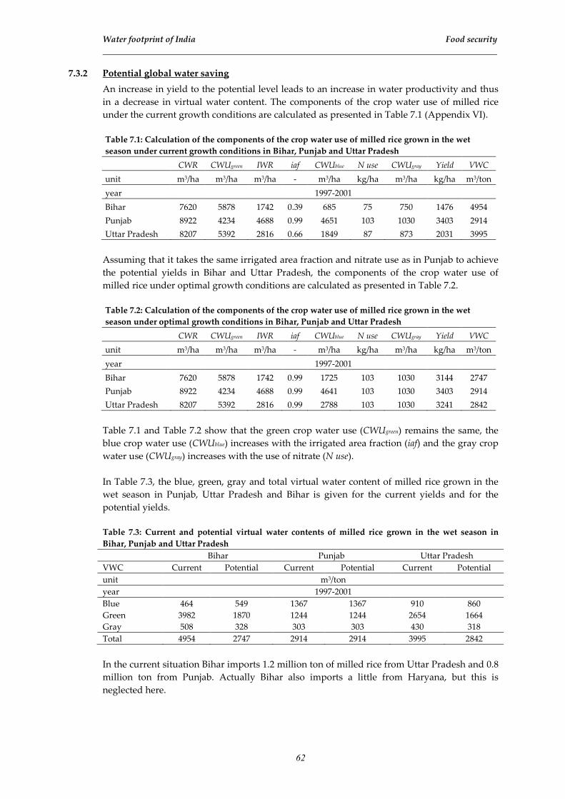
Water footprint of India Food security
62
7.3.2 Potential global water saving
An increase in yield to the potential level leads to an increase in water productivity and thus
in a decrease in virtual water content. The components of the crop water use of milled rice
under the current growth conditions are calculated as presented in Table 7.1 (Appendix VI).
Table 7.1: Calculation of the components of the crop water use of milled rice grown in the wet
season under current growth conditions in Bihar, Punjab and <ttar Pradesh
CWR CWUgreen IWR iaf CWUblue N use CWUgray Yield VWC
unit m3/ha m3/ha m3/ha - m3/ha kg/ha m3/ha kg/ha m3/ton
year 1997-2001
Bihar 7620 5878 1742 0.39 685 75 750 1476 4954
Punjab 8922 4234 4688 0.99 4651 103 1030 3403 2914
Uttar Pradesh 8207 5392 2816 0.66 1849 87 873 2031 3995
Assuming that it takes the same irrigated area fraction and nitrate use as in Punjab to achieve
the potential yields in Bihar and Uttar Pradesh, the components of the crop water use of
milled rice under optimal growth conditions are calculated as presented in Table 7.2.
Table 7.2: Calculation of the components of the crop water use of milled rice grown in the wet
season under optimal growth conditions in Bihar, Punjab and <ttar Pradesh
CWR CWUgreen IWR iaf CWUblue N use CWUgray Yield VWC
unit m3/ha m3/ha m3/ha - m3/ha kg/ha m3/ha kg/ha m3/ton
year 1997-2001
Bihar 7620 5878 1742 0.99 1725 103 1030 3144 2747
Punjab 8922 4234 4688 0.99 4641 103 1030 3403 2914
Uttar Pradesh 8207 5392 2816 0.99 2788 103 1030 3241 2842
Table 7.1 and Table 7.2 show that the green crop water use (CWUgreen) remains the same, the
blue crop water use (CWUblue) increases with the irrigated area fraction (iaf) and the gray crop
water use (CWUgray) increases with the use of nitrate (N use).
In Table 7.3, the blue, green, gray and total virtual water content of milled rice grown in the
wet season in Punjab, Uttar Pradesh and Bihar is given for the current yields and for the
potential yields.
Table 7.3: Current and potential virtual water contents of milled rice grown in the wet season in
Bihar, Punjab and <ttar Pradesh
Bihar Punjab Uttar Pradesh
VWC Current Potential Current Potential Current Potential
unit m3/ton
year 1997-2001
Blue 464 549 1367 1367 910 860
Green 3982 1870 1244 1244 2654 1664
Gray 508 328 303 303 430 318
Total 4954 2747 2914 2914 3995 2842
In the current situation Bihar imports 1.2 million ton of milled rice from Uttar Pradesh and 0.8
million ton from Punjab. Actually Bihar also imports a little from Haryana, but this is
neglected here.

Water footprint of India Food security
63
In Table 7.4, the reduction of the total water use as a result of the current interstate trade is
presented for the current water productivities. Although the situation of food self sufficiency
in Bihar is not possible given the current yield and land availability, this is still assumed in the
calculation to show the reduction of the total water use as a result of interstate trade in the
current situation. In this calculation, the total production and consumption is kept constant.
Table 7.4: Reduction of total water use as a result of current interstate trade with the current water
productivity of milled rice grown in the wet season in Bihar, Punjab and <ttar Pradesh while
keeping the production and consumption constant
States
No interstate trade with current water
productivities
Current interstate trade with current
water productivities reduction
total
water use P1 C2 Water use
P1 C2 Water use
blue green gray total blue green gray total
unit 106 ton/yr 109 m3/yr 106 ton/yr 109 m3/yr %
year 1997-2001
Bihar 7.1 7.1 3.3 28.3 3.6 35.2 5.1 7.1 2.4 20.3 2.6 25.3 T28.1
Punjab 7.7 2.3 10.5 9.6 2.3 22.4 8.5 2.3 11.6 10.6 2.6 24.8 -10.7
UP3 10.7 7.4 9.7 28.4 4.6 42.7 11.9 7.4 10.8 31.6 5.1 47.5 -11.2
Total 25.5 16.8 23.5 66.3 10.5 100.3 25.5 16.8 24.8 62.5 10.3 97.6 T2.7 1 P = production, 2 C = consumption, 3 UP = Uttar Pradesh
Table 7.4 shows that with the current water productivities of milled rice in states involved, the
current interstate trade pattern results in a reduction of the total water use of 2.7%.
In Table 7.5, the reduction of the total water use as a result of the current interstate trade with
the potential water productivities is presented. In this situation, food self sufficiency in Bihar
is realistic given the potential yield and land availability. In this calculation the total
production and consumption is again kept constant.
Table 7.5: Reduction of total water use as a result of current interstate trade with the potential water
productivity of milled rice grown in the wet season in Bihar, Punjab and <ttar Pradesh while
keeping the production and consumption constant
States
No interstate trade with potential water
productivities
Current interstate trade with potential
water productivities reduction
total
water use P1 C2 Water use
P1 C2 Water use
blue green gray total blue green gray total
unit 106 ton/yr 109 m3/yr 106 ton/yr 109 m3/yr %
year 1997-2001
Bihar 7.1 7.1 3.9 13.3 2.3 19.5 5.1 7.1 2.8 9.5 1.7 14.0 T28.2
Punjab 7.7 2.3 10.5 9.6 2.3 22.4 8.5 2.3 11.6 10.6 2.6 24.8 -10.7
UP3 10.7 7.4 9.2 17.8 3.4 30.4 11.9 7.4 10.2 19.8 3.8 33.8 -11.2
Total 25.5 16.8 23.6 40.7 8.0 72.3 25.5 16.8 24.6 39.9 8.1 72.6 -0.4 1 P = production, 2 C = consumption, 3 UP = Uttar Pradesh
Table 7.5 shows that with the potential water productivities of milled rice in states involved,
the current interstate trade results in no reduction of the total water use.
Table 7.6 presents the reduction of the blue, green and gray water use as a result of the
increase in water productivity, in the case of no interstate trade and the current interstate
trade, and as a result of the current interstate trade, for the current and potential water
productivities.

Water footprint of India Food security
64
Table 7.6: Reduction of the blue, green, gray and total water use as a result of current interstate trade
with the current and potential water productivity of milled rice grown in the wet season in Bihar,
Punjab and <ttar Pradesh while keeping the production and consumption constant
Reduction of water use with the
increase in water productivity (%)
Reduction of water use with current
interstate trade of milled rice (%)
No interstate
trade
Current interstate
trade
Current water
productivity
Potential water
productivity
Blue water use -0.4 T0.8 -5.5 -4.2
Green water use T38.6 T36.2 T5.7 T2.0
Gray water use T23.8 T21.4 T1.9 T1.3
Total water use T27.9 T25.6 T2.7 -0.4
Table 7.6 shows that with the increase in water productivity of milled rice grown during the
wet season in Bihar and Uttar Pradesh, a large volume of green and gray water is saved.
Furthermore Table 7.6 shows that the current interstate trade in milled rice from Punjab and
Uttar Pradesh to Bihar results in a green and gray water saving at the cost of a blue water loss.
Table 7.4 and Table 7.5 show that by increasing the water productivities and eliminating the
interstate trade of milled rice between the states involved, a water volume of 25.3 billion m3 is
globally saved. Of this total, 21.8 billion m3 consists of green water saving. The remaining
water saving consists of 1.2 billion m3/yr of blue water and 2.3 billion m3/yr of gray water.
Green water saving may seem useless, as non used green water is lost though evaporation
anyway and therefore has a low opportunity cost. In this example, the area used for milled
rice growth in Bihar is reduced with the new yield and production volume. If the area, which
is not used for milled rice growth anymore, remains unused, the green water saving is
useless. If this area is used for more milled rice production, Rockström (2003) and Rockström
& Gordon (2001, 2002) show that with an increase in yield and a fixed crop area, the total
water productivity remains equal, but the productive part of the water productivity increases.
In this example, this means that a relatively larger fraction of the green water, that is lost
through evapotranspiration, contributes to the biomass of the crop. And by making better use
of green water resources, the crop production can be reduced in places where relatively more
blue water resources are needed for crop growth. In that case relative green water saving
leads to absolute blue water saving.
Apart from resulting in global water saving, the increase in water productivity in combination
with the elimination of the current interstate trade also results in a change in water scarcity in
the states of Bihar, Punjab and Uttar Pradesh. This change in water scarcity from production
and consumption perspective in the states involved is presented in Table 7.7.
Table 7.7: Change in blue, green and total water scarcity from consumption and production
perspective in Bihar, Punjab and <ttar Pradesh with the increase in water productivity combined
with the omission of the current interstate trade in milled rice between the states involved
States
Water scarcity from production perspective1 Water scarcity from consumption perspective1
Current situation2 Potential situation3 Current situation2 Potential situation3
B G T B G T B G T B G T
Bihar 0.03 0.38 0.07 0.03 0.27 0.06 0.05 0.47 0.10 0.04 0.29 0.07
Punjab 0.45 0.65 0.51 0.43 0.61 0.48 0.24 0.32 0.26 0.24 0.32 0.26
UP 0.20 0.43 0.27 0.19 0.34 0.23 0.18 0.34 0.23 0.17 0.29 0.21
1 B = blue water scarcity, G = green water scarcity, T = total water scarcity, 2 Source: Table 6.3, 3 Source: Appendix
XX.
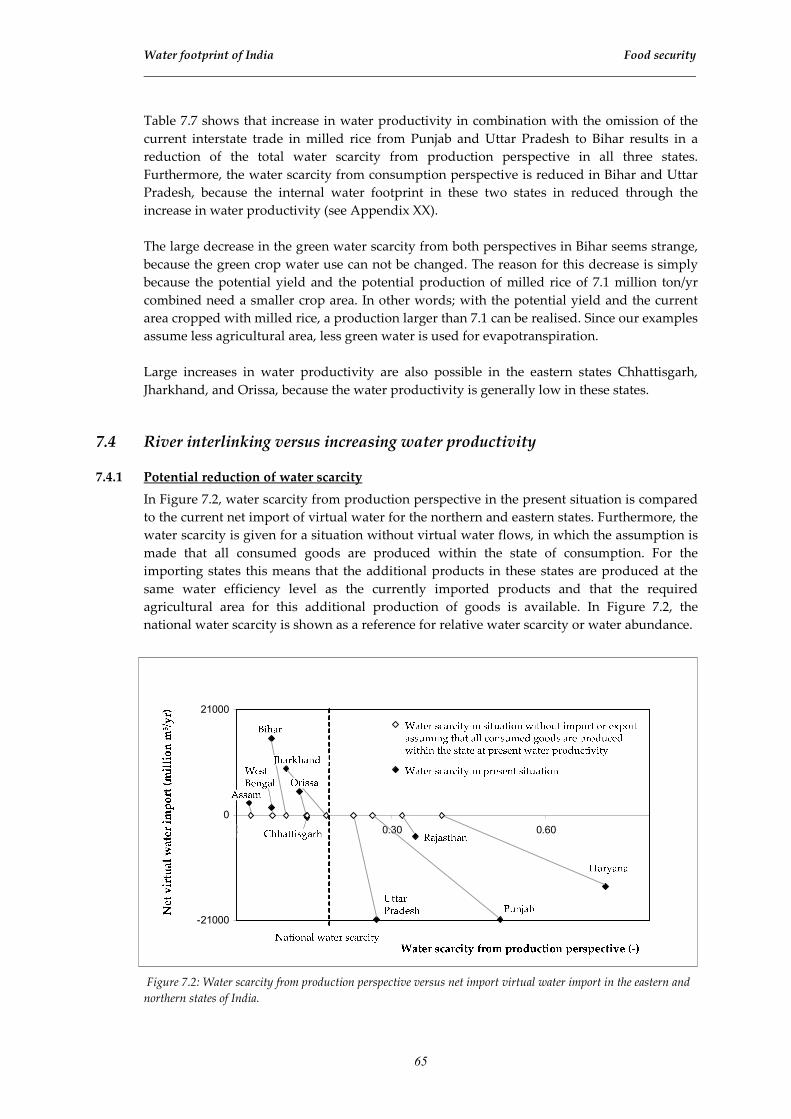
Water footprint of India Food security
65
Table 7.7 shows that increase in water productivity in combination with the omission of the
current interstate trade in milled rice from Punjab and Uttar Pradesh to Bihar results in a
reduction of the total water scarcity from production perspective in all three states.
Furthermore, the water scarcity from consumption perspective is reduced in Bihar and Uttar
Pradesh, because the internal water footprint in these two states in reduced through the
increase in water productivity (see Appendix XX).
The large decrease in the green water scarcity from both perspectives in Bihar seems strange,
because the green crop water use can not be changed. The reason for this decrease is simply
because the potential yield and the potential production of milled rice of 7.1 million ton/yr
combined need a smaller crop area. In other words; with the potential yield and the current
area cropped with milled rice, a production larger than 7.1 can be realised. Since our examples
assume less agricultural area, less green water is used for evapotranspiration.
Large increases in water productivity are also possible in the eastern states Chhattisgarh,
Jharkhand, and Orissa, because the water productivity is generally low in these states.
7.4 River interlinking versus increasing water productivity
7.4.1 Potential reduction of water scarcity
In Figure 7.2, water scarcity from production perspective in the present situation is compared
to the current net import of virtual water for the northern and eastern states. Furthermore, the
water scarcity is given for a situation without virtual water flows, in which the assumption is
made that all consumed goods are produced within the state of consumption. For the
importing states this means that the additional products in these states are produced at the
same water efficiency level as the currently imported products and that the required
agricultural area for this additional production of goods is available. In Figure 7.2, the
national water scarcity is shown as a reference for relative water scarcity or water abundance.
-21000
0
21000
0.00 0.30 0.60
Figure 7.2: Water scarcity from production perspective versus net import virtual water import in the eastern and
northern states of India.

Water footprint of India Food security
66
The gray lines in Figure 7.2 show the development of the water scarcity from production
perspective if the exporting states stop exporting and the importing states start producing all
previously imported goods themselves at the same efficiency as in the current exporting
states. These lines show that the northern states remain relatively water scarce when they stop
exporting virtual water and that the eastern states remain relatively water abundant when
they become food self sufficient, which is line with our findings in Figure 6.4.
Whether real water is transported from east to the north or less virtual water is transported
from the north to the east, both options result in a reduction of water scarcity in the water
scarce northern states at the expense of the water abundant eastern states.
With the execution of the river interlinking project, the national average water scarcity is not
directly changed. This is because the total national water use and total national water
resources are not directly changed. The national water scarcity will only drop if the
production in the areas with high water productivity increases at the cost of the production in
the areas with low water productivity. This can only be realised in case the northern states can
significantly increase their agricultural area. Since it is unclear how much water the northern
states will actually receive through the ILR project, the reduction of the local water scarcity is
hard to estimate. Based on the magnitude of the total water use compared to the magnitude of
the total aimed real water transport, it seems impossible to bring the water scarcity from
consumption perspective in the northern states below the national water scarcity with the ILR
project.
With the increase in water productivity in the water abundant states in combination with the
elimination of the virtual water flows between the north and the east, the national average
water scarcity can be reduced significantly. This is because the increase in water productivity
reduces the total water footprint and therefore reduces the national water scarcity.
In Figure 7.3, the four possible combinations of water scarcity from production perspective
and net import of virtual water in a state are given. Here, a state is water abundant when the
water scarcity in that state is below the national water scarcity and a state is water scarce
when the water scarcity in that state is above the national water scarcity. Figure 7.3 also shows
the consequences of the following strategies; the interlinking of rivers to transport water from
water abundant areas to water scarce areas (A), the reduction of the food export in the water
scarce states and of food import in the water abundant states (B), and the increase in water
productivity (C).

Water footprint of India Food security
67
Water abundant stateswith net importof virtual water
Water abundant stateswith net exportof virtual water
Water scarce states with net importof virtual water
Water scarce stateswith net exportof virtual water
Net virtual water import
Net virtual water export
Water scarce
Water abundant
A,C
B
B
A,C
AC
BBTC
BTC B
A
C
Figure 7.3: The four combinations of water scarcity and net import of virtual water and the consequences of the
following strategies; the interlinking of rivers to transport water from water abundant areas to water scarce areas
(A), the reduction of the food export in the water scarce states and of food import in the water abundant states (B),
and the increase in water productivity (C).
Figure 7.3 shows that strategy A (ILR project) reduces the water scarcity in the water scarce
states at the cost of the water abundant states. However, this is not enough to shift these states
from water scarce to water abundant. Furthermore, Figure 7.3 shows that a combination of
strategy B and strategy C reduces the water scarcity in the water scarce states and keeps the
water scarcity in the water abundant states more or less constant, which means that the
national water scarcity is reduced.
As can be seen in Figure 7.3, the ILR project does not change the illogical situation from a
water management perspective. Since the volume of water that can be transported is limited,
the northern states can not become water abundant states. In order to change the illogical
situation in which a large part of the water abundance in the eastern states is unutilized, the
eastern states have to change from importing virtual water to exporting virtual water. If the
agricultural area cannot be expanded, the only way to achieve this is to increase the water
productivity.
So all in all, the ILR project reduces local water scarcity, but will not significantly reduce the
national water scarcity. Furthermore, in the case of milled rice, a trade flow is currently
maintained that causes a global saving of green and gray water, but a global loss of blue
water.
From the perspective of logical water management, the transport of (blue) water only seems
useful when a virtual water flow is maintained that results in global blue water saving.
Yang (2003) indicates that there is a water resources threshold with respect to the import of
cereals. Below this threshold, cereal import demand will increase exponentially with the
decrease of the water availability per capita. This would mean that the northern states
eventually are bound to reduce their export of virtual water and maybe even start importing
virtual water.

Water footprint of India Food security
68
7.5 Water saving by changing crop patterns
Finally, after presenting the option of reducing or increasing crop production and changing
the direction of trade, the option of changing crop patterns in order to achieve global water
saving is briefly discussed here.
The theory of comparative advantage is used here to evaluate changes in crop patterns in the
Indian states. The three important parameters in this evaluation are the potential yield, the
water requirement and the water productivity of a crop.
In Figure 7.4, the possible relation between the total water availability and the crop yield of
two crops is shown. Here, the potential yield is found when the water availability equals the
crop water requirement. The steepness of the curve represents the water productivity.
Aie
ld
Figure 7.4: The possible relation between the total water availability for evapotranspiration and the crop yield for
two crops in a state
Figure 7.4 shows a situation in which crop 1 generates a higher yield in states with a relatively
low water availability and crop 2 generates a higher yield in states with a relatively high
water availability.
When two crops are compared to each other, the boundary condition is that the crops are
competitive. In the case of green water use, crops are only competitive if they are grown in the
same season under comparable conditions. In the case of blue water use, crops can also be
competitive if they are not grown in the same season, because blue water, especially in the
form of groundwater, is available over a longer time period.
In this study we have seen that in the current situation a large amount of milled rice as well as
wheat is annually exported from Punjab and Uttar Pradesh to Bihar. Based on the theory of
comparative advantage, Bihar must have a relative advantage in water productivity for one of
these two crops. Because milled rice and wheat are not grown in during the same season, we
only compare blue and gray water use.
The opportunity costs of milled rice and wheat in the states Bihar, Punjab and Uttar Pradesh
are presented in Table 7.8.

Water footprint of India Food security
69
Table 7.8: Opportunity costs of milled rice and wheat in the states Bihar, Punjab and <ttar Pradesh
with the exclusion of green water productivity in the present situation during the period 1997-2001
Crops Opportunity costs
Bihar Punjab Uttar Pradesh
Unit -
1.00 ton of milled rice 0.72 ton of wheat 3.00 ton of wheat 1.09 ton of wheat
1.00 ton of wheat 1.39 ton of milled rice 0.33 ton of milled rice 0.92 ton of milled rice
From Table 7.8, the conclusion can be carefully made that Bihar currently has a relative
advantage in blue and gray water productivity of milled rice when compared to Punjab and
Uttar Pradesh. This means that the current trade flows of milled rice from Punjab and Uttar
Pradesh to Bihar do not save water according to the theory of comparative advantage. It is
worth noticing that the relative advantage in water productivity of a crop may change when
the calculation is made for potential crop yields instead of actual crop yields. In this case this
is not likely to happen, as Bihar receives significantly more green water than Punjab and Uttar
Pradesh in the wet season, and therefore requires relatively less blue water for rice growth,
and receives less green water than Punjab and Uttar Pradesh in the dry season, and therefore
requires relatively more blue water for wheat growth.
Of course it is still too early to make such a conclusion. We just want to indicate that a state
like Bihar currently has no significant crop export, while there must be a crop in which Bihar
has the highest relative advantage in water productivity.
When looking at the current trade patterns and the theory of comparative advantage in the
present situation, it might be useful to include the yield response factor of a crop in the
analysis. The yield response factor is a constant that determines the sensitivity of the crop
yield to water deficit (Doorenbos & Kassam, 1979).
The comparison of relative advantages in water productivities of crops might not be sufficient
to determine the optimal policies for maximizing the social benefits from limited water
resources (Wichelns, 2001). This means that the availability of labour, capital and land in a
state should also be taken into account in the calculation of relative advantages in water
productivity of crops. This is because water is not always the limiting factor for the increase in
crop production. In Bihar for example, there is enough water and labour, but the production
is limited by the availability of land and capital.

70
71
8. Conclusion and discussion
8.1 Conclusion
In the period 1997-2001, the total virtual water flow as a result of interstate trade in
agricultural commodities in India was 106 billion m3/yr, which was equal to 13% of the total
water use in Indian agriculture. In the same period, the net international export from India
was 15 billion m3/yr. A comparable study for China showed a total virtual water flow
between Chinese sub-regions of billion 128 m3/yr in the year 1999, which was equal to 10% of
the total agricultural water use in China (Ma et al., 2006). In the period 1997-2001, the global
sum of international virtual water flows related to the trade of agricultural commodities was
987 billion m3/yr (Chapagain and Hoekstra, 2004). Of the total virtual water flow within India,
35% is due to the interstate trade of milled rice, 17% due the interstate trade of raw sugar and
14% due to the interstate trade of edible oils. The largest interregional net virtual water flow is
22 billion m3/yr and flows from the North India to the East India. As a result of international
and interstate virtual water flows, the states Haryana, Madhya Pradesh, Punjab and Uttar
Pradesh relatively have the largest negative virtual water balance and Bihar, Jharkhand and
Kerala relatively have the largest positive virtual water balance.
During our study period, the average water footprint of the consumption of agricultural
commodities in India was 777 m3/cap/yr. In the same period, the average global water
footprint of the consumption of agricultural commodities was 1066 m3/cap/yr, which did not
include gray water use. The internal component is responsible for 658 m3/cap/yr and the
external component for 119 m3/cap/yr. Furthermore, the blue component came to 227
m3/cap/yr, the green component to 459 m3/cap/yr and the gray component to 92 m3/cap/yr. A
significant relation is visible between high water footprints and poor agricultural practice in
the Indian states. The states Chhattisgarh and Orissa have the highest water footprint, which
is mainly because of the low water productivity in the local rice production.
For India as a whole, the water use from consumption perspective (777 billion m3/yr) was
very close to the water use from production perspective (792 billion m3/yr). However, for
individual states, like Bihar and Punjab, the consumption perspective often provides a very
new picture if compared to the traditional production perspective.
From the perspective of consumption, the water scarcity is the highest in the Rajasthan,
Punjab, Uttar Pradesh, Tamil Nadu and Haryana. This means that the water resources of
these states are closest to be exhausted in case of food self sufficiency. Because most of these
states are also net exporters of virtual water, the water scarcity from a production perspective
is even higher in these states.
The total net global water saving as a result of the interstate trade in agricultural commodities
in India was 41 billion m3/yr. This means the total water use in Indian agriculture was 5%

Water footprint of India Conclusion and discussion
72
lower than it would have been without interstate trade. The interstate trade in wheat alone
already caused a global water saving of 23 billion m3/yr.
It must be noted that the above mentioned numbers are somewhat uncertain, as this study is
based on approximately 77% of the total crop production, 61% of the total production value
and 84% of the total agricultural land use in India.
Currently, India is considering implementing the concept of river interlinking. This concept
means that water abundant regions will provide water to water scarce regions through the
connection of rivers. Looking at the interlinking project from the perspective of the virtual
water flows as calculated in this study, it can be seen that the proposed water transfer from
East to North India has a direction exactly opposite to the direction of the virtual water flow
as a result of interstate trade. In this study, it is demonstrated that an increase in water
productivity in the water abundant states has a better chance of reducing the national water
scarcity than the proposed water transfer. The river interlinking project mainly reduces local
water scarcity, while water scarcity needs to be reduced significantly at a national level in
order to remain food self sufficient as a nation. The only long term option for reducing the
national water scarcity and remaining food self sufficient is to increase the water productivity
in India. The largest opportunity for this increase lies in East India, where there is an
abundance of water and a large increase in water productivity seems possible.
8.2 Discussion
The methodology used in this study is largely based on earlier studies, which already
calculated international virtual water flows and water footprints of nations (Hoekstra &
Chapagain, 2007), virtual water flows and water footprints within a nation (Ma et al., 2006),
the water footprint of a product (Chapagain et al., 2006) and global water saving as a result of
international trade (Chapagain & Hoekstra, 2006). In this study, these previous methodologies
are integrated and upgraded where possible. The main upgrades are the incorporation and
assessment of green and blue water resources and the demonstration of how a consumption
perspective on water management can quantitatively dispute water management strategies
that are determined with a production perspective.
The data that is used and generated in this study are rough and in some cases not complete.
The roughness is due to the large scale of the study areas. Since one set of climatic parameters
per state is used and only one set of crop parameters for whole India per season, the
calculated virtual water content of crops do catch the main regional patterns but seem quite
unreliable in the case of rain fed crops grown during the dry season. An incompleteness of
this study is due the exclusion of crops. Important crops like coconuts, mango and pimento
still represent a significant part of the total water use.
Furthermore, the livestock products are excluded from this study. During the study period
livestock products contributed a small part to the total water use in Indian agriculture. But the
production and interstate of especially milk is increasing quickly. For example, Gujarat has an
enormous milk production and where Gujarat in this study is assessed as an importer of
virtual water, the inclusion of milk might well turn Gujarat into a net exporter of virtual
water.
The external water resources are very roughly estimated. The influence of large hill ranges
like the Western Ghats are not taken into account. And in the assessment of the current water

Water footprint of India Conclusion and discussion
73
scarcity, the determination of the utilizable fraction of the total water resources will improve
the reliability of the water scarcity at state level.
This study covers the period 1997-2001 and since patterns of crop production and crop trade
change in time as a result of the average increase in welfare, the data that is used and
generated might become less suitable to describe the present and future situations.
By only looking at virtual water, the social benefits from limited water resources will not be
maximized. So the fact that we are only looking at water resources is a limitation to this study.
The availability of labour, capital and land should therefore be included in the relative
advantage of the water productivity of crops. This might also change the importance of
certain crops, which might not require much water, but may require much labour, land or
capital. However, since the food self sufficiency is projected to become critical in the future,
the present point of view is important for the future of India.
It could be argued that the importance of water is small compared to the importance of land,
labour, energy and capital. For example, irrigation in Bihar is currently executed with diesel
pumps while in Punjab electricity is available, which is much cheaper. Water is a relatively
costless resource, while products with virtual water embodied in it are seen as relatively
costly. In other words; the import of real water feeds the perception of self sufficiency,
whereas the import of virtual water feeds the perception of dependency.
This study also misses a more detailed case study, which would have given a better insight in
the practical implementation possibilities of both the river interlinking project and the
increase in water productivity.
Still we feel that this study gives a good indication of the virtual water flows in India, because
it is indisputable that the direction of the largest virtual water flow is opposite to the direction
of the aimed real water transport and that the water productivity in East India still has a large
gap with the potential water productivity. In general, we can also dispute whether the
exclusion of the alternative of national virtual water import to meet the increasing food
demand is a smart move, because whatever internal solution will be chosen to meet the food
demand in the future in India, the average water availability per capita in India will keep
dropping with the increase in population.

74

75
References
Aggarwal, P.K., Talukdar, K.K., Mall, R.K., 2000. Potential yields of rice-wheat system in the Indo-
Gangetic Plains if India. Consortium Paper Series 10. Rice-wheat consortium for the Indo-Gangetic
Plains, New Delhi.
Agrawal, G.D., 1999. Diffuse agricultural water pollution in India. Water Science and Technology, Vol.
39, p.33-47.
Allan, J.A., 1993. Fortunately there are substitutes for water otherwise our hydro-political futures would
be impossible. In: Priorities for water resources allocation and management, ODA, London, p. 13-26.
Allan, J.A., 1994. Overall perspectives on countries and regions. In: Rogers, P., Lydon, P. (editors). Water
in the Arab World: perspectives and prognoses. Harvard University Press, Cambridge, Massachusetts,
p. 65-100.
Allen, R.G., Pereira, L.S., Raes, D. and Smith, M., 1998. Crop evapotranspiration – Guidelines for
computing crop water requirements. FAO Irrigation and Drainage Papers, Vol. 56, FAO, Rome, Italy.
Bobba, A.G., Singh, V.P., Bengtsson, L., 1997. Sustainable Development of Water Resources in India.
Environmental Management, Vol. 21, p. 367-393.
CDC, 2007. The Centers for Disease Control and Prevention, Atlanta, USA. www.cdc.gov/epiinfo/asia.htm
Census of India, 2006. Census Data online. Registrar General and Census Commissioner, Government of
India, New Delhi. http://www.censusindia.net
CGWD, 1989. Ground water statistics. Central Groundwater Board, Ministry of Irrigation and Power,
Department of Irrigation, Ministry of water resources, Government of India, Faridabad.
Chandigarh Administration, 2006. Statistics. Chandigarh Administration, Chandigarh.
http://sampark.chd.nic.in/images/statistics/SDP2005R6.pdf
Chapagain, A.K., Hoekstra, A.Y., 2003. Virtual water flows between nations in relation to trade in
livestock and livestock products. Value of Water Research Report Series No. 13, UNESCO-IHE Institute
for Water Education, Delft, the Netherlands. http://www.waterfootprint.org/Reports/Report13.pdf
Chapagain, A.K, Hoekstra, A.Y., 2004. Water footprints of nations. Value of Water Research Report
Series No. 16, UNESCO-IHE Institute for Water Education, Delft, the Netherlands.
http://www.waterfootprint.org/Reports/Report16Vol1.pdf
Chapagain, A.K., Hoekstra, A.Y., 2006. Water saving through international trade of agricultural
products. Hydrol. Earth Syst. Sci., 10, p.455-468.
Chapagain, A.K., Hoekstra, A.Y., Savenije, H.H.G., Gautam, R., 2006. The water footprint of cotton
consumption: An assessment of the impact of worldwide consumption of cotton products on the water
resources in the cotton producing countries. Ecological Economics 60, p. 186-203.
Chaturvedi, M.C., 1985. Water resources of India – an overview. Sadhana. Vol. 8, p. 13-38.

Water footprint of India References
76
CIA, 2006. The World Factbook. Central Intelligence Agency, Government of United States of America,
Washington D.C. https://www.cia.gov/cia/publications/factbook/geos/in.html
Dastane, N.G., 1978. Effective rainfall in irrigated agriculture. FAO Irrigation and Drainage Papers. Vol.
25, FAO, Rome, Italy.
Directorate of Economics and Statistics, 2003. Agricultural Statistics at a Glance. Agricultural Statistics
Division, Directorate of Economics and Statistics, Ministry of Agriculture, Government of India, New
Delhi.
Directorate of Economics and Statistics, 2004. Agricultural Statistics at a Glance. Agricultural Statistics
Division, Directorate of Economics and Statistics, Ministry of Agriculture, Government of India, New
Delhi.
Directorate of Rice Development, 2006a. Status Paper on Rice. Ministry of Agriculture, Government of
India, Patna. http://www.dacnet.nic.in/rice
Directorate of Rice Development, 2006b. Statistical Handbook. Ministry of Agriculture, Government of
India, Patna. http://www.dacnet.nic.in/rice
Directorate of Rice Development, 2006c. Productivity Analysis. Ministry of Agriculture, Government of
India, Patna. http://www.dacnet.nic.in/rice
Directorate of Pulses Development, 2006a. Varieties of pulses. Ministry of Agriculture, Government of
India, Bhopal. http://dacnet.nic.in/pulses/APY-website.pdf
Directorate of Pulses Development, 2006b. Statistics. Ministry of Agriculture, Government of India,
Bhopal. http://dacnet.nic.in/pulses/ VARIETIES-Web%20site.pdf
Directorate of Wheat Development, 2006. Statistics. Ministry of Agriculture, Government of India,
Ghaziabad. http://dacnet.nic.in/dwd/wheat_prod1/wheat-annx3.pdf
Dohlman, E., Persaud, S., Landes, R., 2003. India’s Edible Oil Sector: Imports Fill Rising Demand. United
States Department of Agriculture, Washington D.C.
Doorenbos, J., Kassam, A.H., 1979. Yield Response to Water. FAO Irrigation and Drainage Papers. Vol.
33, FAO, Rome, Italy. http://www.fao.org/AG/AGL/aglw/cropwater/part.stm
EPA, 2006. List of drinking water contaminants: groundwater and drinking water. US Environmental
Protection Agency, Washington D.C.
Falkenmark, M., Rockström, J., 1993. Curbing rural exodus from tropical drylands. Ambio 22, p.427-437.
Falkenmark, M., 1997. Meeting water requirements of an expanding world population. Phil. Trans. R.
Soc. Lond. B. 352, p. 929-936.
Falkenmark, M., Lannerstad, M., 2005. Consumptive water use to feed humanity – curing the blind spot.
Hydrology and Earth System Sciences, Vol.9, p. 15-28.
FAO, 2003. Review of the World Water Resources by Country. Water Reports 23. Food and Agricultural
Organization of the United Nations, Rome, Italy.
FAO, 2005. Fertilizer use by crop in India. Food and Agricultural Organization of the United Nations,
Rome, Italy.
FAO, 2006a. ‘FAOSTAT on-line database’, Food and Agriculture Organization of the United Nations,
Rome, Italy

Water footprint of India References
77
FAO, 2006b. CROPWAT model. Food and Agriculture Organization of the United Nations, Rome, Italy.
http://www.fao.org/ag/AGL/aglw/cropwat.stm
FAO, 2006c. CLIMWAT database. Food and Agriculture Organization of the United Nations, Rome,
Italy. http://www.fao.org/ag/AGL/aglw/climwat.stm
FAO, 2006d. Technical Conversion Factors for Agricultural Commodities. Food and Agriculture
Organization of the United Nations, Rome, Italy.
http://www.fao.org/WAICENT/FAOINFO/ECONOMIC/ESS/pdf/tcf.pdf
FAO, 2006e. AQUASTAT database, Food and Agriculture Organization of the United Nations, Rome,
Italy
FAORAP, 2006. Regional Data Exchange System on food and Agricultural Statistics in Asia and the
Pacific Countries. Regional Office for Asia and the Pacific, Food and Agricultural Organization,
Bangkok, Thailand.
Gupta, S.K., Deshpande, R.D., 2004. Water for India in 2050: first-order assessment of available options.
Current Science, Vol.86, No.9.
Hoekstra, A.Y., Chapagain, A.K., 2007. Water footprints of nations: Water use by people as function of
their consumption pattern. Water Resources Management 21, p.35-48.
Hoekstra, A.Y., Hung, P.Q., 2004. Globalisation of water resources: international virtual water flows in
relation to crop trade. Global Environmental Change 15, p.45-56.
IISR, 2006. Statistics. Indian Institute of Sugar Cane Research, Lucknow. http://iisr.nic.in
IITM, 2006. Data. Indian Institute of Tropical Meteorology, Pune. http://www.tropmet.res.in
IMD, 2006. Normal rainfall maps. India Meteorological Department, New Delhi.
http://www.imd.ernet.in/section/climate/annual-rainfall.htm
Ma, J., Hoekstra, A.Y., Wang, H., Chapagain, A.K., Wang, D., 2006. Virtual versus real water transfers
within China. Phil.Trans.R.Soc.B., Vol.361, p.835-842.
Ministry of Water Resources, 2006a. Ground Water pollution. Ministry of Water Resources, Government
of India, New Delhi.
Ministry of Water Resources, 2006b. Water statistics. Ministry of Water Resources, Government of India,
New Delhi.
Ministry of Water Resources, 2006c. River basin maps. Ministry of Water Resources, Government of
India, New Delhi.
NSSO, 1997. Consumption of Some Important Commodities in India 1993-1994. National Sample Survey
Organisation Report 404, Department of Statistics, Ministry of Statistics & Programme Implementation,
Government of India, New Delhi.
NSSO, 1998. Household Consumer Expenditure and Employment Situation in India in 1997. National
Sample Survey Organisation Report 442, Department of Statistics, Ministry of Statistics & Programme
Implementation, Government of India, New Delhi.
NSSO, 1999. Household Consumer Expenditure and Employment Situation in India in 1998. National
Sample Survey Organisation Report 448, Department of Statistics, Ministry of Statistics & Programme
Implementation, Government of India, New Delhi.

Water footprint of India References
78
NSSO, 2001a. Level and Pattern of Consumer Expenditure in India 1999-2000. National Sample Survey
Organisation Report 457, Department of Statistics, Ministry of Statistics & Programme Implementation,
Government of India, New Delhi.
NSSO, 2001b. Consumption of Some Important Commodities in India 1999-2000. National Sample
Survey Organisation Report 461, Department of Statistics, Ministry of Statistics & Programme
Implementation, Government of India, New Delhi.
NSSO, 2002. Household Consumer Expenditure and Employment – Unemployment Situation in India
2000-2001. National Sample Survey Organisation Report 476, Department of Statistics, Ministry of
Statistics & Programme Implementation, Government of India, New Delhi.
NSSO, 2003. Household Consumer Expenditure and Employment – Unemployment Situation in India
2001-2002. National Sample Survey Organisation Report 481, Department of Statistics, Ministry of
Statistics & Programme Implementation, Government of India, New Delhi.
NSSO, 2005. Sarvekshana, Journal of National Sample Survey Organisation, 88th Issue Vol XXV No.4 &
Vol XXVI Vol.1. Department of Statistics, Ministry of Statistics & Programme Implementation,
Government of India, New Delhi.
NWDA, 2006. Inter Basin Water Transfer Proposals. National Water Development Agency. A Society
under Ministry of Water Resources, Government of India, New Delhi.
Phansalkar, S.J., Verma, S., 2005. Mainstreaming the Margins – Water-centric Livelihood Strategies for
Revitalizing Tribal Agriculture in Central India. Angus & Grapher, New Delhi.
Planning Commission, 2002. Tenth Five Year Plan 2002-2007. Planning Commission, Government of
India, New Delhi. http://planningcommission.nic.in/
Postel, S.L., Daily, G.C., Ehrlich, P.R., 1996. Human Appropriation of Renewable Fresh Water. Science,
Vol. 271, p.785-788.
Price, G.K., Landes, R., Govindan, A., 2003. India’s Pulse Sector: Results of Field Research. United States
Department of Agriculture, Washington D.C.
Radhakrishna, B.P., 2003. Linking of major rivers of India – Bane or boon? Current Science, Vol. 84, p.
1390-1394.
Rao, K.L., 1973. India’s Water Wealth. Orient Longman, New Delhi.
Ricardo, D., 1817. On the Principles of Political Economy and Taxation. John Murray, Albemarle-street,
London.
Rockström, J., Gordon, L., 2001. Assessment of Green Water Flows to Sustain Major Biomes of the
World: Implications for Future Ecohydrological Landscape Management. Phys. Chem. Earth (B), Vol.26,
No.11-12, p. 843-851.
Rockström, J., Gordon, L., 2002. The Role of Green Water in Sustaining Ecological Functions – A Global
Assessment. Water and Ecology, GAIA 11, No.4, p.267-272.
Rockström, J., 2003. Water for food and nature in drought-prone tropics: vapour shift in rain-fed
agriculture. Phil. Trans. R. Soc. Lond. B. 358, p. 1997–2009.
Rosegrant, M.V., Cai, X., Cline, S.A., 2002. World Water and Food to 2025. International Food Policy
Research Institute, Washington D.C., USA.

Water footprint of India References
79
United Nations, 2004. World population prospects: The 2004 Revision, Volume III: Analytical Report.
United Nations Department of Economic and Social Affairs, New York, USA.
Wackerhagel, M., Rees, W., 1996. Our ecological footprint: Reducing human impact on the Earth. New
Society Publishers, Gabriola Island, BC, Canada.
Wichelns, D., 2001. The role of ‘virtual water’ in efforts to achieve food security and other national goals,
with an example from Egypt. Agricultural Water Management 49, p.131-151.
Wichelns, D., 2007. Virtual Water: An Economic Perspective. In: Trimble, S.W. (ed.) Encyclopedia of
Water Science, Taylor & Francis, New York. Article in press.
World Bank, 2006. India at a Glance 2005. Data & Statistics, World Bank, Washington D.C., USA.
http://siteresources.worldbank.org/INTSARMACECOGRO/34004333-1148990480174/21048623/India.pdf
Yang, H., Reichert, P., Abbaspour, K.C., Zehnder, A.J.B., 2003. A Water Resources Threshold and Its
Implications for Food Security. Environmental Science & Technology. Vol. 37, p. 3048-3054.

Appendices
Appendix I. Symbols ............................................................................................................. A-1
Appendix II. Area and population of the Indian states .................................................... A-3
Appendix III. Crop production India .................................................................................... A-5
Appendix IV. List of weather stations ................................................................................... A-7
Appendix V. Crop parameters ............................................................................................. A-10
Appendix VI. Product and value fractions ......................................................................... A-11
Appendix VII. National crop balances ................................................................................. A-12
Appendix VIII. Virtual water contents of crops ................................................................... A-13
Appendix IX. Comparison of calculated gray water use to nitrate use by state .......... A-26
Appendix X. Sensitivity analysis of virtual water content of kharif milled rice ....... A-27
Appendix XI. Production, consumption and surplus of crops ....................................... A-28
Appendix XII. Assessment of interstate and international crop trade ........................... A-31
Appendix XIII. Interstate virtual water flows by colour .................................................... A-37
Appendix XIV. Water footprints by colour ........................................................................... A-42
Appendix XV. Water footprints compared to consumption volume and climate ........ A-44
Appendix XVI. Other estimates on the water resources of India...................................... A-45
Appendix XVII. Average annual precipitation ...................................................................... A-46
Appendix XVIII. Water resources of the Indian states .......................................................... A-47
Appendix XIX. Blue water flows between the Indian states ............................................. A-48
Appendix XX. Assessment of water scarcity in a potential situation ............................. A-54


A-1
Appendix I. Symbols
Symbol Unit Description
CWR m3/ha Crop water requirement of crop c per crop period
ETc,opt mm/day Crop evapotranspiration with an abundance of water
Kc - Crop coefficient
ET0 mm/day Reference evapotranspiration
CWUgreen m3/ha Green crop water use
ETc,rw mm/day Crop evapotranspiration under rain fed conditions
Peff mm/day Effective rainfall
Ptot mm/day Total rainfall
CWUblue m3/ha Blue crop water use
ETc,iw mm/day Crop evapotranspiration of irrigation water
IWR mm/day Irrigation water requirement
iaf - Irrigated area fraction
ETc,act mm/day Total actual crop evapotranspiration
CWUtot m3/ha Total actual crop water use
WD - Water deficit during crop growth
DWR m3/ha Dilution water requirement
Nleached ton/ha Amount of nitrate that leaches to groundwater
df m3/ton Dilution factor
Nused ton/ha Amount of nitrate supplied to the field
lf - Leaching factor
rl mg/l Recommended level of nitrogen
VWCtot m3/ton Total virtual water content of a crop
VWCblue m3/ton Blue virtual water content of a crop
VWCgreen m3/ton Green virtual water content of a crop
VWCgray m3/ton Gray virtual water content of a crop
Yc ton/ha Yield of a crop
pf - Product fraction of a processed product
vf - Value fraction of a processed product
VWCpc m3/ton Virtual water content of a processed product
WP ton/m3 Water productivity of a crop
AWU m3/yr Total agricultural water use
P ton/yr Production volume
AWUblue m3/yr Blue agricultural water use
AWUgreen m3/yr Green agricultural water use
AWUgray m3/yr Gray agricultural water use
St ton/yr Total supply volume of a crop
Ut ton/yr Total utilization volume of a crop
Pt ton/yr Total production volume of a crop
It,in ton/yr Total international import volume of a crop
SIt ton/yr Total stock increase volume of a crop
SDt ton/yr Total stock decrease volume of a crop
Et,in ton/yr Total international export volume of a crop
Fdt ton/yr Total animal feed volume of a crop
Sdt ton/yr Total seed volume of a crop
Mt ton/yr Total manufacture volume of a crop
Wt ton/yr Total waste volume of a crop
Out ton/yr Total other use volume of a crop
Ct ton/yr Total consumption volume of a crop
Ss ton/yr State supply volume of a crop
Us ton/yr State utilization volume of a crop
Ps ton/yr State production volume of a crop
Is,in ton/yr State international import volume of a crop
Is,is ton/yr State interstate import volume of a crop

A-2
SIs ton/yr State stock increase volume of a crop
SDs ton/yr State stock decrease volume of a crop
Es,in ton/yr State international export volume of a crop
Es,is ton/yr State interstate export volume of a crop
Fds ton/yr State animal feed volume of a crop
Sds ton/yr State seed volume of a crop
Ms ton/yr State manufacture volume of a crop
Ws ton/yr State waste volume of a crop
Ous ton/yr State other use volume of a crop
Cs ton/yr State consumption volume of a crop
Tt,is ton/yr Total interstate trade of a crop
Sps ton/yr State surplus of a crop
RUt ton/yr Total remaining utilizations of a crop
VWFs m3/yr Virtual water flow as a result of crop trade between two states
VWFs,tot m3/yr Total virtual water flow as a result of interstate trade of a crop
VWInet m3/yr Net virtual water balance of a state
WFPtot m3/yr Total water footprint
WFPi m3/yr Internal water footprint
WFPe m3/yr External water footprint
VWEgross m3/yr Gross export of virtual water
VWIgross m3/yr Gross import of virtual water
WFPcap m3/cap/yr Total water footprint per capita
Pop capita Population
Qin m3/yr Total volume of water flowing into a state
Qout m3/yr Total volume of water flowing out of a state
ETtot m3/yr Total volume of evapotranspiration within a state
Qe m3/yr Total outflow of external water from a state
Qi m3/yr Total inflow of external water in a state
NAWUgreen m3/yr Total use of rain water in non agricultural areas
WRgreen m3/yr Total green water resources
Anon,agric ha/yr Total non agricultural area
WRblue,i m3/yr Internal blue water resources
As,rb ha Area of state in a river basin
Arb ha Area of river basin
As ha Area of state
Qi,rb m3/yr Contribution of internal water resources to river basin discharge
Qout,rb m3/yr Total outflow of water from a state
Qin,rb m3/yr Total inflow of external water into a state in a river basin
WRblue,e m3/yr External blue water resources
WRblue,tot m3/yr Total blue water resources
WRtot m3/yr Total water resources
Qrb m3/yr Total discharge volume of state s
WSprod - Total water scarcity from a production perspective
WSprod,green - Green water scarcity from a production perspective
WSprod,blue - Blue water scarcity from a production perspective
WScons - Total water scarcity from a consumption perspective
WScons,green - Green water scarcity from a consumption perspective
WScons,blue - Blue water scarcity from a consumption perspective
ΔSs m3/yr State water saving as a result of import of a crop
ΔSg m3/yr Global water saving as result of interstate trade of a crop
WPET mm Total water productivity
WPT mm Productive part of water productivity

A-3
Appendix II. Area and population of the Indian
states
Area, population and population density of the Indian states and union territories
State/ Union Territory1 Abbrev.2 Area3 Population4 Population
density5 rural urban total
unit km² 1000 capita cap/km2
year 1997-2001
Andaman & Nicobar ANI 8,249 234 111 346 42
Andhra Pradesh AP 275,068 54,127 19,963 74,083 269
Arunachal Pradesh ARP 83,743 850 219 1,067 13
Assam AS 78,483 22,682 3,299 25,911 330
Bihar BH 94,164 72,608 8,329 80,682 857
Chandigarh CDG 144 90 776 875 6,080
Chhattisgarh CG 135,194 16,265 4,015 20,252 150
Dadra & Nagar Haveli DNH 491 166 48 214 437
Daman & Diu DMD 122 99 55 154 1,261
Delhi DL 1,483 923 12,381 13,464 9,079
Goa GOA 3,702 662 643 1,310 354
Gujarat GJ 196,024 31,011 18,160 49,257 251
Haryana HR 44,212 14,684 5,867 20,554 465
Himachal Pradesh HP 55,673 5,356 571 5,908 106
Jammu & Kashmir JK 222,236 7,452 2,414 9,861 44
Jharkhand JH 79,700 20,470 5,750 26,194 329
Karnataka KT 191,791 34,087 17,231 51,375 268
Kerala KL 38,863 23,032 7,931 30,953 796
Lakshadweep LSW 32 33 26 59 1,842
Madhya Pradesh MP 308,144 43,360 15,318 58,663 190
Maharashtra MH 307,713 54,495 39,429 94,174 306
Manipur MNP 22,327 1,554 553 2,106 94
Meghalaya MGL 22,429 1,822 436 2,254 100
Mizoram MIZ 21,081 437 423 864 41
Nagaland NGL 16,579 1,609 329 1,934 117
Orissa OR 155,707 30,568 5,293 35,777 230
Pondicherry PDC 492 318 622 947 1,925
Punjab PJ 50,362 15,726 7,926 23,679 470
Rajasthan RJ 342,236 42,297 12,677 54,930 161
Sikkim SIK 7,096 470 57 526 74
Tamil Nadu TN 130,058 34,119 26,366 60,664 466
Tripura TRP 10,492 2,592 524 3,110 296
Uttar Pradesh UP 238,566 128,630 33,135 161,558 677
Uttaranchal UA 53,566 6,165 2,090 8,252 154
West Bengal WB 88,752 56,421 21,515 77,938 878
All India 3,284,974 725,415 274,482 999,896 304
Total included in study 3,087,995 714,478 269,660 984,129 319
94% 98% 98% 98%
1 The shaded states and union territories are excluded from this study, 2 Abbrev. = the abbreviations of the states
and union territories used in this study, 3 Source: en.wikipedia.org, 4 Source: Census of India (2006), FAO (2006), 5 Population density = total population divided by state area.
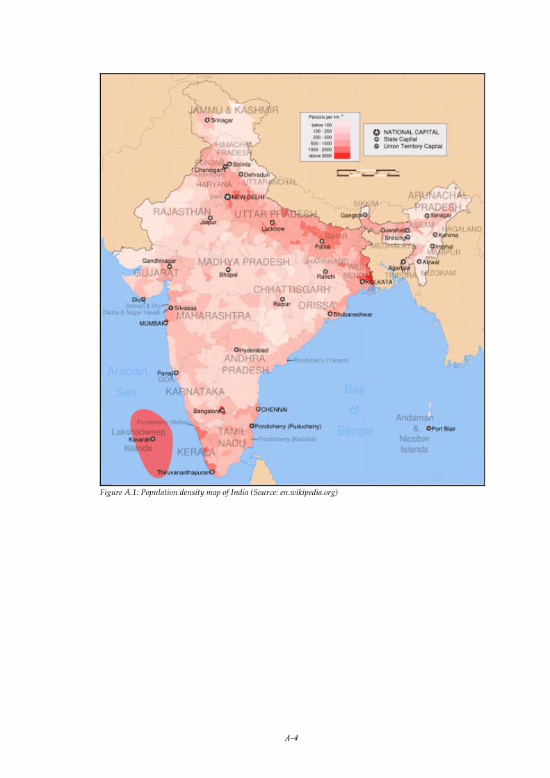
A-4
Figure A.1: Population density map of India (Source: en.wikipedia.org)

A-5
Appendix III. Crop production India
Primary crops CC1 P2 VWC3 WU4 PP5 VP6 LU7
unit 103
ton/yr m3/ton
Gm3/
yr %
US$/
ton
109
US$/yr %
106
ha/yr %
year 1997-2001
Rice, Paddy C 130903 2850 373.1 39.3 126 16.5 21.4 44.6 25.0
Wheat C 70606 1654 116.8 12.3 148 10.4 13.5 26.7 15.0
Seed Cotton OC 5716 8264 47.2 5.0 509 2.9 3.8 8.9 5.0
Sugar Cane SC 286042 159 45.6 4.8 18 5.1 6.7 4.1 2.3
Millet C 10162 3269 33.2 3.5 101 1.0 1.3 12.6 7.0
Sorghum C 7990 4053 32.4 3.4 118 0.9 1.2 10.1 5.7
Soybeans OC 6364 4124 26.2 2.8 232 1.5 1.9 6.3 3.5
Groundnuts in Shell OC 6991 3420 23.9 2.5 327 2.3 3.0 6.8 3.8
Maize C 11764 1937 22.8 2.4 115 1.3 1.7 6.4 3.6
Beans, Dry P 2609 8335 21.7 2.3 292 0.8 1.0 6.7 3.8
Coconuts OC 9345 2255 21.1 2.2 87 0.8 1.1 1.8 1.0
Mangoes F 10582 1525 16.1 1.7 359 3.8 4.9 1.4 0.8
Chick-Peas P 5494 2712 14.9 1.6 352 1.9 2.5 6.8 3.8
Rapeseed OC 5400 2618 14.1 1.5 313 1.7 2.2 6.1 3.4
Pimento, Allspice SP 953 11126 10.6 1.1 850 0.8 1.1 0.9 0.5
Pigeon Peas P 2433 4066 9.9 1.0 380 0.9 1.2 3.5 1.9
Castor Beans OC 794 9807 7.8 0.8 277 0.2 0.3 0.8 0.4
Fruit Fresh nes8 F 6424 1066 6.9 0.7 214 1.4 1.8 0.7 0.4
Cashew Nuts TN 444 15340 6.8 0.7 728 0.3 0.4 0.7 0.4
Bananas F 15574 415 6.5 0.7 140 2.2 2.8 0.5 0.3
Lentils P 940 6652 6.3 0.7 311 0.3 0.4 1.4 0.8
Tea nes8 ST 832 7002 5.8 0.6 186 0.2 0.2 0.5 0.3
Vegetables Fresh nes8 V 25772 207 5.3 0.6 158 4.1 5.3 2.1 1.2
Jute VF 1729 2823 4.9 0.5 200 0.3 0.4 0.8 0.4
Sesame Seed OC 579 8415 4.9 0.5 441 0.3 0.3 1.6 0.9
Potatoes SR 22535 213 4.8 0.5 107 2.4 3.1 1.3 0.7
Natural Rubber R 583 7626 4.4 0.5 701 0.4 0.5 0.4 0.2
Sunflower Seed OC 780 4304 3.4 0.4 372 0.3 0.4 1.4 0.8
Spices nes8 SP 799 4054 3.2 0.3 488 0.4 0.5 1.0 0.6
Areca Nuts (Betel) TN 322 9985 3.2 0.3 1279 0.4 0.5 0.3 0.2
Pulses nes8 P 1043 3078 3.2 0.3 500 0.5 0.7 1.8 1.0
Coffee, Green ST 258 12180 3.1 0.3 1553 0.4 0.5 0.3 0.2
Fruit Trop. Fresh nes7 F 2810 1104 3.1 0.3 214 0.6 0.8 0.3 0.2
Barley C 1511 1966 3.0 0.3 124 0.2 0.2 0.8 0.4
Linseed OC 264 11080 2.9 0.3 343 0.1 0.1 0.7 0.4
Onions, Dry V 4931 538 2.7 0.3 115 0.6 0.7 0.5 0.3
Apples F 1256 1812 2.3 0.2 498 0.6 0.8 0.2 0.1
Tomatoes V 7232 302 2.2 0.2 149 1.1 1.4 0.4 0.2
Peas, Dry P 707 3040 2.1 0.2 234 0.2 0.2 0.6 0.4
Cassava SR 6549 283 1.9 0.2 67 0.4 0.6 0.2 0.1
Safflower Seed OC 251 6864 1.7 0.2 295 0.1 0.1 0.4 0.2
Tobacco Leaves T 602 2627 1.6 0.2 508 0.3 0.4 0.4 0.2
Oilseeds nes8 OC 147 8023 1.2 0.1 327 0.0 0.1 0.5 0.3
Nutmeg, Cardamoms SP 13 90511 1.1 0.1 1762 0.0 0.0 0.1 0.1
Eggplants V 7728 146 1.1 0.1 - - 0.0 0.5 0.3
Jute-Like Fibres VF 199 5295 1.1 0.1 200 0.0 0.1 0.1 0.0
Oranges F 2842 364 1.0 0.1 360 1.0 1.3 0.1 0.1
Cabbages V 5428 180 1.0 0.1 121 0.7 0.8 0.2 0.1
Pumpkins, Gourds V 3400 238 0.8 0.1 - - 0.0 0.4 0.2
Lemons, Limes F 1298 611 0.8 0.1 262 0.3 0.4 0.1 0.1

A-6
Primary crops CC1 P2 VWC3 WU4 PP5 VP6 LU7
unit 103
ton/yr m3/ton
Gm3/
yr %
US$/
ton
109
US$/yr %
106
ha/yr %
year 1997-2001
Anise, Badian, Fennel SP 110 7063 0.8 0.1 513 0.1 0.1 0.3 0.2
Garlic V 514 1268 0.7 0.1 486 0.2 0.3 0.1 0.1
Papayas F 652 922 0.6 0.1 182 0.1 0.2 0.1 0.0
Okra V 3442 168 0.6 0.1 - - 0.0 0.3 0.2
Pepper White/Black SP 61 8333 0.5 0.1 2982 0.2 0.2 0.2 0.1
Peas, Green V 2766 178 0.5 0.1 273 0.8 1.0 0.3 0.2
Cauliflower V 4736 100 0.5 0.0 244 1.2 1.5 0.3 0.1
Ginger SP 263 1556 0.4 0.0 356 0.1 0.1 0.1 0.0
Walnuts TN 28 11721 0.3 0.0 1077 0.0 0.0 0.0 0.0
Pineapples F 1063 305 0.3 0.0 190 0.2 0.3 0.1 0.0
Sweet Potatoes SR 1076 277 0.3 0.0 108 0.1 0.2 0.1 0.1
Grapes F 1039 238 0.2 0.0 341 0.4 0.5 0.0 0.0
Pears F 175 1287 0.2 0.0 199 0.0 0.0 0.0 0.0
Lettuce V 778 258 0.2 0.0 - - 0.0 0.1 0.1
Beans, Green V 412 487 0.2 0.0 158 0.1 0.1 0.1 0.1
Peaches, Nectarines F 117 1564 0.2 0.0 174 0.0 0.0 0.0 0.0
Plums F 73 1907 0.1 0.0 174 0.0 0.0 0.0 0.0
Watermelons F 252 362 0.1 0.0 87 0.0 0.0 0.0 0.0
Cocoa Beans ST 6 13775 0.1 0.0 - - 0.0 0.0 0.0
Cantaloupes, Melons F 642 115 0.1 0.0 525 0.3 0.4 0.0 0.0
Carrots V 344 192 0.1 0.0 319 0.1 0.1 0.0 0.0
Citrus Fruit nes8 F 116 528 0.1 0.0 235 0.0 0.0 0.0 0.0
Grapefruit, Pomelos F 120 411 0.0 0.0 174 0.0 0.0 0.0 0.0
Cucumbers, Gherkins V 118 357 0.0 0.0 - - 0.0 0.0 0.0
Apricots F 9 2424 0.0 0.0 174 0.0 0.0 0.0 0.0
Figs F 10 2147 0.0 0.0 174 0.0 0.0 0.0 0.0
Cherries F 7 2532 0.0 0.0 631 0.0 0.0 0.0 0.0
Chillies/Peppers, Green V 49 285 0.0 0.0 850 0.0 0.1 0.0 0.0
Stone Fruit nes, Fresh8 F 1 1434 0.0 0.0 - - 0.0 0.0 0.0
Berries nes8 F 1 897 0.0 0.0 - - 0.0 0.0 0.0
All crops 718914 949.0 100 77.1 100 178.3 100
1 CC= crop categories; C = cereals, OC = oil crops, SC = sugar crops, P = pulses, F = fruits, SP = spices, TN = tree
nuts, ST = stimulants, V = vegetables, VF = vegetable fibres, SR = starchy roots, R = rubber and T = tobacco. 2 P =
National crop production, source: FAOSTAT (FAO, 2006), 3 VWC = Virtual water content of crop, source:
Chapagain and Hoekstra (2004) 4 WU = Water use, which is the production times virtual water content, 5 PP =
producer price (US$ 1997-2001), source: FAOSTAT (FAO, 2006), for a few crops this value is not given, 6 VP =
Value of production, which is the production times producer price, 7 LU = Land use, source: FAOSTAT (FAO,
2006), 8 Nes = not elsewhere specified.

A-7
Appendix IV. List of weather stations
MEASUREMENT
STATION DISTRICT
STATE / UNION
TERRITORY
ALTITUDE
(m)
LATITUDE
(o,/)
LONGITUDE
(o,/)
AGRA AGRA UTTAR PRADESH 169 27.1 78.02
AHMADABAD AHMADABAD GUJARAT 55 23.04 72.38
AHMADNAGAR AHMADNAGAR MAHARASHTRA 657 19.05 74.48
AJMER AJMER RAJASTHAN 486 26.27 74.37
AKOLA AKOLA MAHARASHTRA 282 20.42 77.02
ALIBAG RAIGARH MAHARASHTRA 7 18.38 72.52
ALIGARH ALIGARH UTTAR PRADESH 187 27.53 78.04
ALLABABAD ALLAHABAD UTTAR PRADESH 98 25.27 81.44
AMBALA AMBALA HARYANA 272 30.23 76.46
AMINI (N/A) LAKSHADWEEP 4 11.07 72.44
AMRAOTI AMRAVATI MAHARASHTRA 370 20.56 77.47
AMRITSAR AMRITSAR PUNJAB 234 31.38 74.52
ANGUL DHENKANAL ORISSA 139 20.5 85.06
ASANSOL BARDDHAMAN WEST BENGAL 126 23.41 86.58
AURANGABAD AURANGABAD MAHARASHTRA 581 19.53 75.2
BAHRAICH BAHRAICH UTTAR PRADESH 124 27.34 81.36
BALASORE BALESHWAR ORISSA 20 21.31 86.56
BALEHONNUR CHIKMAGALUR KARNATAKA 889 13.22 75.27
BANGALORE BANGLORE KARNATAKA 921 12.58 77.35
BAREILLY BAREILLY UTTAR PRADESH 173 28.22 79.24
BARMER BARMER RAJASTHAN 194 25.45 71.23
BARODA VADODARA GUJARAT 34 22.18 73.15
BELGAUM BELGAUM KARNATAKA 753 15.51 74.32
BELLARY BELLARY KARNATAKA 449 15.09 76.51
BERHAMPORE MURSHIDABAD WEST BENGAL 19 24.08 88.16
BHAVNAGAR (AERO) BHAVNAGAR GUJARAT 11 21.45 72.11
BHOPAL (BAIRAGARH) SEHORE MADHYA PRADESH 523 23.17 77.21
BHUJ (RUDRAMATA) KACHCHH GUJARAT 80 23.15 69.4
BIDAR BIDAR KARNATAKA 664 17.55 77.32
BIJAPUR BIJAPUR KARNATAKA 594 16.49 75.43
BIKANER BIKANER RAJASTHAN 224 28 73.18
BOMBAY GREATER BOMBAY MAHARASHTRA 11 18.54 72.49
BURDWAN BARDDHAMAN WEST BENGAL 32 23.14 87.51
CALCUTTA (DUM DUM) 24 PARGANAS WEST BENGAL 6 22.39 88.26
CHAIBASA SINGHBHUM JHARKHAND 226 22.33 85.49
CHANDBALI BALESHWAR ORISSA 6 20.47 86.44
CHANDRAPUR CHANDRAPUR MAHARASHTRA 193 19.58 79.18
CHERRAPUNJI (N/A) MEGHALAYA 1313 25.15 91.44
CHITRADURGA CHITRADURGA KARNATAKA 733 14.14 76.26
COCHIN ERNAKULAM KERALA 3 9.58 76.14
COIMBATORE COIMBATORE TAMIL NADU 409 11 78.58
COONOOR NILGIRI TAMIL NADU 1747 11.21 76.48
CUDDALORE SOUTH ARCOT TAMIL NADU 12 11.46 79.46
CUDDAPAH CUDDAPAH ANDHRA PRADESH 130 14.29 78.5
CUTTACK CUTTACK ORISSA 27 20.28 85.56
DALTONGANJ PALAMU JHARKHAND 221 24.03 84.04
DARBHANGA DARBHANGA BIHAR 49 26.1 85.54
DARJEELING DARJEELING WEST BENGAL 2127 27.03 88.16
DEHRA DUN DEHRADUN UTTARANCHAL 682 30.19 78.02
DHAMBAD DHANBAD JHARKHAND 257 23.47 86.26
DHUBRI (N/A) ASSAM 35 26.01 89.58
DIBRUGARH (N/A) ASSAM 110 27.29 95.01
DOHAD DAHOD GUJARAT 333 22.5 74.16
DUMKA DUMKA JHARKHAND 149 24.16 87.15
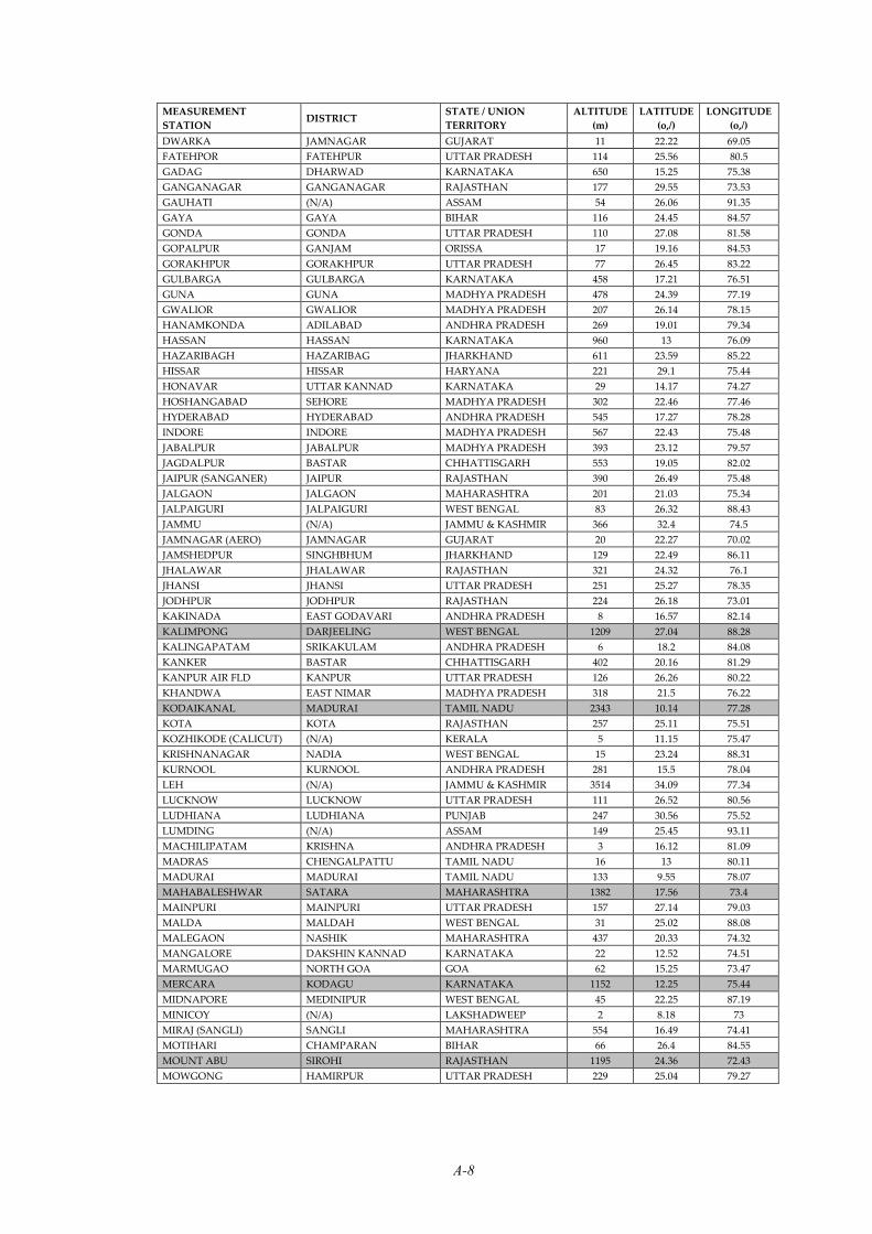
A-8
MEASUREMENT
STATION DISTRICT
STATE / UNION
TERRITORY
ALTITUDE
(m)
LATITUDE
(o,/)
LONGITUDE
(o,/)
DWARKA JAMNAGAR GUJARAT 11 22.22 69.05
FATEHPOR FATEHPUR UTTAR PRADESH 114 25.56 80.5
GADAG DHARWAD KARNATAKA 650 15.25 75.38
GANGANAGAR GANGANAGAR RAJASTHAN 177 29.55 73.53
GAUHATI (N/A) ASSAM 54 26.06 91.35
GAYA GAYA BIHAR 116 24.45 84.57
GONDA GONDA UTTAR PRADESH 110 27.08 81.58
GOPALPUR GANJAM ORISSA 17 19.16 84.53
GORAKHPUR GORAKHPUR UTTAR PRADESH 77 26.45 83.22
GULBARGA GULBARGA KARNATAKA 458 17.21 76.51
GUNA GUNA MADHYA PRADESH 478 24.39 77.19
GWALIOR GWALIOR MADHYA PRADESH 207 26.14 78.15
HANAMKONDA ADILABAD ANDHRA PRADESH 269 19.01 79.34
HASSAN HASSAN KARNATAKA 960 13 76.09
HAZARIBAGH HAZARIBAG JHARKHAND 611 23.59 85.22
HISSAR HISSAR HARYANA 221 29.1 75.44
HONAVAR UTTAR KANNAD KARNATAKA 29 14.17 74.27
HOSHANGABAD SEHORE MADHYA PRADESH 302 22.46 77.46
HYDERABAD HYDERABAD ANDHRA PRADESH 545 17.27 78.28
INDORE INDORE MADHYA PRADESH 567 22.43 75.48
JABALPUR JABALPUR MADHYA PRADESH 393 23.12 79.57
JAGDALPUR BASTAR CHHATTISGARH 553 19.05 82.02
JAIPUR (SANGANER) JAIPUR RAJASTHAN 390 26.49 75.48
JALGAON JALGAON MAHARASHTRA 201 21.03 75.34
JALPAIGURI JALPAIGURI WEST BENGAL 83 26.32 88.43
JAMMU (N/A) JAMMU & KASHMIR 366 32.4 74.5
JAMNAGAR (AERO) JAMNAGAR GUJARAT 20 22.27 70.02
JAMSHEDPUR SINGHBHUM JHARKHAND 129 22.49 86.11
JHALAWAR JHALAWAR RAJASTHAN 321 24.32 76.1
JHANSI JHANSI UTTAR PRADESH 251 25.27 78.35
JODHPUR JODHPUR RAJASTHAN 224 26.18 73.01
KAKINADA EAST GODAVARI ANDHRA PRADESH 8 16.57 82.14
KALIMPONG DARJEELING WEST BENGAL 1209 27.04 88.28
KALINGAPATAM SRIKAKULAM ANDHRA PRADESH 6 18.2 84.08
KANKER BASTAR CHHATTISGARH 402 20.16 81.29
KANPUR AIR FLD KANPUR UTTAR PRADESH 126 26.26 80.22
KHANDWA EAST NIMAR MADHYA PRADESH 318 21.5 76.22
KODAIKANAL MADURAI TAMIL NADU 2343 10.14 77.28
KOTA KOTA RAJASTHAN 257 25.11 75.51
KOZHIKODE (CALICUT) (N/A) KERALA 5 11.15 75.47
KRISHNANAGAR NADIA WEST BENGAL 15 23.24 88.31
KURNOOL KURNOOL ANDHRA PRADESH 281 15.5 78.04
LEH (N/A) JAMMU & KASHMIR 3514 34.09 77.34
LUCKNOW LUCKNOW UTTAR PRADESH 111 26.52 80.56
LUDHIANA LUDHIANA PUNJAB 247 30.56 75.52
LUMDING (N/A) ASSAM 149 25.45 93.11
MACHILIPATAM KRISHNA ANDHRA PRADESH 3 16.12 81.09
MADRAS CHENGALPATTU TAMIL NADU 16 13 80.11
MADURAI MADURAI TAMIL NADU 133 9.55 78.07
MAHABALESHWAR SATARA MAHARASHTRA 1382 17.56 73.4
MAINPURI MAINPURI UTTAR PRADESH 157 27.14 79.03
MALDA MALDAH WEST BENGAL 31 25.02 88.08
MALEGAON NASHIK MAHARASHTRA 437 20.33 74.32
MANGALORE DAKSHIN KANNAD KARNATAKA 22 12.52 74.51
MARMUGAO NORTH GOA GOA 62 15.25 73.47
MERCARA KODAGU KARNATAKA 1152 12.25 75.44
MIDNAPORE MEDINIPUR WEST BENGAL 45 22.25 87.19
MINICOY (N/A) LAKSHADWEEP 2 8.18 73
MIRAJ (SANGLI) SANGLI MAHARASHTRA 554 16.49 74.41
MOTIHARI CHAMPARAN BIHAR 66 26.4 84.55
MOUNT ABU SIROHI RAJASTHAN 1195 24.36 72.43
MOWGONG HAMIRPUR UTTAR PRADESH 229 25.04 79.27
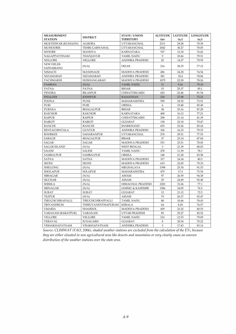
A-9
MEASUREMENT
STATION DISTRICT
STATE / UNION
TERRITORY
ALTITUDE
(m)
LATITUDE
(o,/)
LONGITUDE
(o,/)
MUKTESWAR (KUMAON) ALMORA UTTARANCHAL 2311 29.28 79.39
MUSSOORIE TEHRI GARWAHAL UTTARANCHAL 2042 30.27 78.05
MYSORE MANDYA KARNATAKA 767 12.18 76.42
NAGAPPATTINAM THANJAVUR TAMIL NADU 9 10.46 79.51
NELLORE NELLORE ANDHRA PRADESH 20 14.27 79.59
NEW DELHI-
SAFDARJANG (N/A) DELHI 216 28.35 77.12
NIMACH MANDSAUR MADHYA PRADESH 496 24.28 74.54
NIZAMABAD NIZAMABAD ANDHRA PRADESH 381 18.4 78.06
PACHMARHI HOSHANGABAD MADHYA PRADESH 1075 22.28 78.26
PAMBAN (N/A) TAMIL NADU 11 9.16 79.18
PATNA PATNA BIHAR 53 25.37 85.1
PENDRA BILASPUR CHHATTISGARH 625 22.46 81.54
PHALODI JODHPUR RAJASTHAN 234 27.08 72.22
POONA PUNE MAHARASHTRA 559 18.32 73.51
PURI PURI ORISSA 6 19.48 85.49
PURNEA BHAGALPUR BIHAR 38 25.16 87.28
RAICHOR RAICHOR KARNATAKA 400 16.12 77.21
RAIPUR RAIPUR CHHATTISGARH 298 21.14 81.39
RAJKOT RAJKOT GUJARAT 138 22.18 70.47
RANCHI RANCHI JHARKHAND 655 23.26 85.24
RENTACHINTALA GUNTUR ANDHRA PRADESH 106 16.33 79.33
ROORKEE SAHARANPUR UTTARANCHAL 274 29.51 77.53
SABAUR BHAGALPUR BIHAR 37 25.14 87.04
SAGAR SAGAR MADHYA PRADESH 551 23.51 78.45
SAGAR ISLAND (N/A) WEST BENGAL 3 21.39 88.03
SALEM SALEM TAMIL NADU 278 11.39 78.1
SAMBALPUR SAMBALPUR ORISSA 148 21.28 83.58
SATNA SATNA MADHYA PRADESH 317 24.34 80.5
SEONI SEONI MADHYA PRADESH 619 22.05 79.33
SHILLONG (N/A) MEGHALAYA 1598 25.34 91.53
SHOLAPUR SOLAPUR MAHARASHTRA 479 17.4 75.54
SIBSAGAR (N/A) ASSAM 97 26.59 94.38
SILCHAR (N/A) ASSAM 29 24.49 92.48
SHIMLA (N/A) HIMACHAL PRADESH 2202 31.06 77.1
SRINAGAR (N/A) JAMMU & KASHMIR 1586 34.05 74.5
SURAT SURAT GUJARAT 12 21.12 72.5
TEZPUR (N/A) ASSAM 79 26.37 92.47
TIRUCHCHIRAPALLI TIRUCHCHIRAPPALLI TAMIL NADU 88 10.46 78.43
TRIVANDRUM THIRUVANENTHAPURAM KERALA 64 8.29 76.57
UMARIA SHAHDOL MADHYA PRADESH 459 23.32 80.53
VARANASI (BABATPUR) VARANASI UTTAR PRADESH 85 25.27 82.52
VELLORE VELLORE TAMIL NADU 214 12.55 79.09
VERAVAL JUNAGARH GUJARAT 8 20.54 70.22
VISHAKHAPATNAM VISAKHAPATNAM ANDHRA PRADESH 3 17.43 83.14
Source: CLIMWAT (FAO, 2006), shaded weather stations are excluded from the calculation of the ET0, because
they are either situated in non agricultural area like deserts and mountains or very clearly cause an uneven
distribution of the weather stations over the state area.
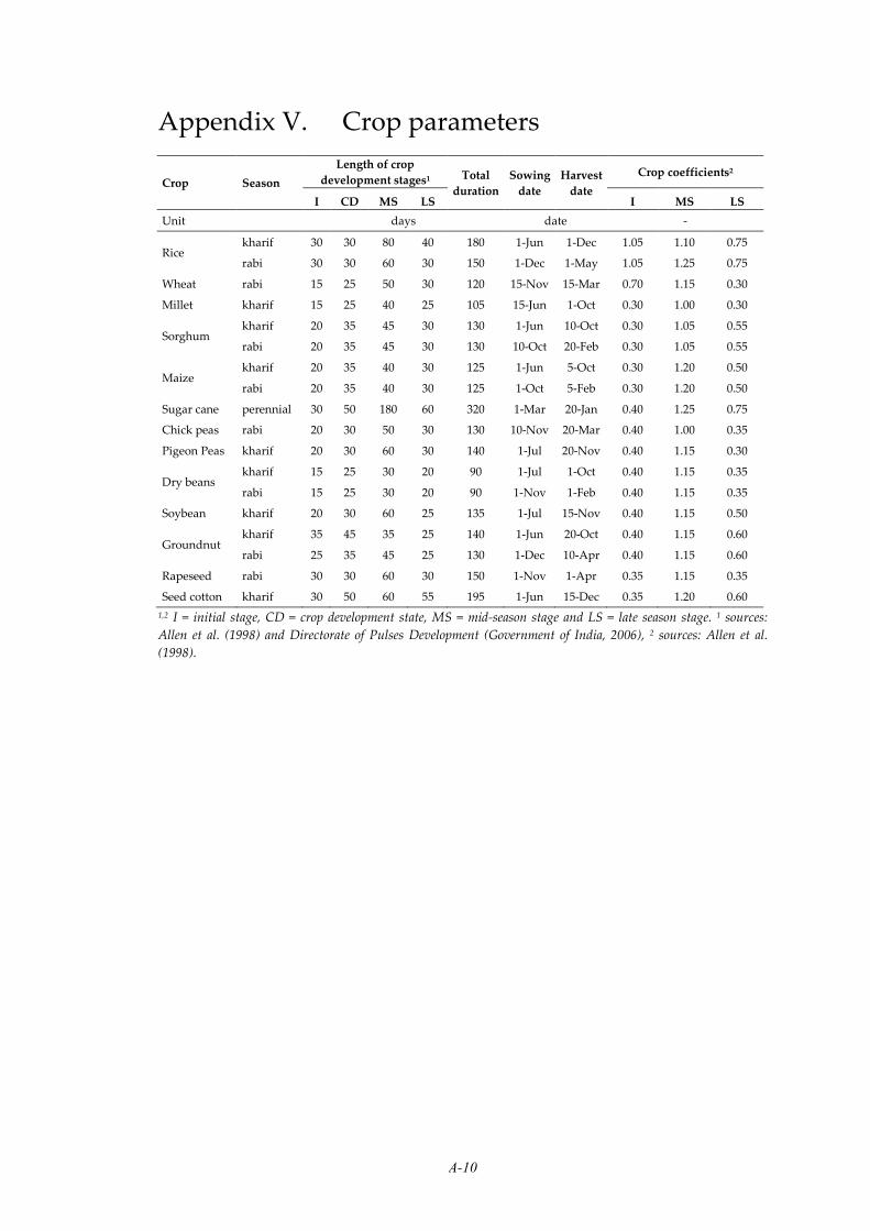
A-10
Appendix V. Crop parameters
Crop Season
Length of crop
development stages1 Total
duration
Sowing
date
Harvest
date
Crop coefficients2
I CD MS LS I MS LS
Unit days date -
Rice kharif 30 30 80 40 180 1-Jun 1-Dec 1.05 1.10 0.75
rabi 30 30 60 30 150 1-Dec 1-May 1.05 1.25 0.75
Wheat rabi 15 25 50 30 120 15-Nov 15-Mar 0.70 1.15 0.30
Millet kharif 15 25 40 25 105 15-Jun 1-Oct 0.30 1.00 0.30
Sorghum kharif 20 35 45 30 130 1-Jun 10-Oct 0.30 1.05 0.55
rabi 20 35 45 30 130 10-Oct 20-Feb 0.30 1.05 0.55
Maize kharif 20 35 40 30 125 1-Jun 5-Oct 0.30 1.20 0.50
rabi 20 35 40 30 125 1-Oct 5-Feb 0.30 1.20 0.50
Sugar cane perennial 30 50 180 60 320 1-Mar 20-Jan 0.40 1.25 0.75
Chick peas rabi 20 30 50 30 130 10-Nov 20-Mar 0.40 1.00 0.35
Pigeon Peas kharif 20 30 60 30 140 1-Jul 20-Nov 0.40 1.15 0.30
Dry beans kharif 15 25 30 20 90 1-Jul 1-Oct 0.40 1.15 0.35
rabi 15 25 30 20 90 1-Nov 1-Feb 0.40 1.15 0.35
Soybean kharif 20 30 60 25 135 1-Jul 15-Nov 0.40 1.15 0.50
Groundnut kharif 35 45 35 25 140 1-Jun 20-Oct 0.40 1.15 0.60
rabi 25 35 45 25 130 1-Dec 10-Apr 0.40 1.15 0.60
Rapeseed rabi 30 30 60 30 150 1-Nov 1-Apr 0.35 1.15 0.35
Seed cotton kharif 30 50 60 55 195 1-Jun 15-Dec 0.35 1.20 0.60
1,2 I = initial stage, CD = crop development state, MS = mid-season stage and LS = late season stage. 1 sources:
Allen et al. (1998) and Directorate of Pulses Development (Government of India, 2006), 2 sources: Allen et al.
(1998).

A-11
Appendix VI. Product and value fractions
Product and value fractions of the processed crops in India
Primary crop Processed product Product fraction1 Value fraction2
Year 1997-2001
Paddy rice Milled rice3 0.66 1.00
Wheat4 - 1.00 1.00
Maize4 - 1.00 1.00
Millet4 - 1.00 1.00
Sorghum4 - 1.00 1.00
Sugar cane Raw sugar5 0.105 1.00
Chickpeas6 - 1.00 1.00
Pigeon peas6 - 1.00 1.00
Dry beans6 - 1.00 1.00
Soybean Soybean oil7 0.18 0.34
Soybean Soybean cake 0.79 0.66
Groundnut in shell Groundnut shelled 0.705 1.00
Groundnut shelled Groundnut oil7 0.415 1.00
Rapeseed Rapeseed oil7 0.344 1.00
Coconut Coconut oil7 0.12 -
Sunflower seed Sunflower seed oil7 0.368 -
Seed cotton Cottonseed 0.67 0.21
Seed cotton Cotton lint 0.33 0.79
Cottonseed Cottonseed oil7 0.14 1.00
1 Source: FAO (2006). 2 Source: Chapagain and Hoekstra (2004). 3 Because of annual changes between the volumes of processed rice products, the product fraction of the milled rice
equivalent might change in time. The product fraction that is used for the milled rice equivalent in India is 0.66. 4 Wheat, maize, millet and sorghum are generally consumed in the form of flour, which has a product fraction
lower than 1 (0.98 for whole grain wheat flour, 0.80 for maize flour, 0.93 for millet flour and 0.95 for sorghum
flour). But in this study the consumption is given in the primary equivalent, which means the product fraction of
these grains are 1.00. 5 The average global fraction of sugar cane that ends up in the form of raw sugar is 0.10. For India this product
fraction of the raw sugar equivalent is the same. 6 In general, pulses are consumed as a whole, which means a product fraction of 1.00. Only in the case of chickpeas,
approximately 50% is consumed in the form of flour known as besan (Price et al., 2003). This flour has a product
fraction of 0.80. In this study, this fact is not taken into account, which means all pulses are assumed to have a
product fraction of 1.00. 7 The product fractions of the edible oils are directly taken from the crop balances. These are found by dividing the
volume of oil produced by the volume of the primary crop that is manufactured.

A-12
Appendix VII. National crop balances
Products1 Domestic supply2 Domestic utilization3 Per
capita
P I ΔS E DS Fd Sd M W Ou C C
Unit 1000 ton/yr kg/yr
Year 1997-2001
Rice, milled equivalent 87317 25 -3858 2606 80878 349 4694 4 872 30 74929 74.9
Wheat 70607 943 -4632 850 66067 847 4816 5 2995 0 57404 57.4
Maize 11735 75 0 40 11770 4780 707 3 1278 46 4956 5.0
Millet 10123 0 0 12 10110 162 361 0 497 0 9091 9.1
Sorghum 7943 0 0 0 7943 95 293 0 543 0 7011 7.0
Sugar cane 288202 0 0 0 288202 2957 19021 253254 0 0 12969 13.0
Sugar, non centrifugal4 9008 0 9008 450 8558 8.6
Sugar, raw equivalent4 17469 524 -1244 422 16327 4 16324 16.3
Pulses5 13349 931 0 175 14105 1202 719 0 457 0 11727 11.7
Soybean6 6385 7 -580 40 5772 0 376 4810 294 0 292 0.3
Soybean oil 867 607 -22 6 1447 0 0 0 0 0 1447 1.4
Groundnut shelled 4941 0 -8 154 4779 20 323 3902 148 0 385 0.4
Groundnut oil 1621 0 -40 0 1581 0 0 0 0 0 1581 1.6
Sunflower seed oil7 281 312 -2 1 589 0 0 0 0 32 557 0.6
Rape and mustard seed 5400 2 0 3 5399 0 41 4819 162 0 377 0.4
Rape and mustard oil 1656 122 -3 2 1772 0 0 0 0 8 1764 1.8
Cottonseed 3696 0 0 0 3696 609 174 2728 185 0 0 0.0
Cottonseed oil 382 27 -7 0 402 0 0 0 0 0 402 0.4
Coconut oil7 422 19 -4 3 433 0 0 0 0 13 420 0.4
Palm oil7 0 2608 -98 25 2485 0 0 0 0 438 2048 2.0 1 The national crop balances are taken from food balance sheets of FAO (2006), since cotton lint is not considered
as food, this crop is excluded. 2 P = domestic crop production, I = crop import , ΔS = crop withdrawn from domestic stocks, E = crop export, DS
= domestic supply (=P+I+ΔS-E). 3 Fd = feed (amount of crop for livestock and poultry feeding), Sd = seed use (amount of crop set aside for
reproduction purposes), M = crop manufacture (amount of crop which is further processed), W = crop waste, Ou =
other crop use, C = human crop consumption. 4 FAO divides sugar from sugar cane in centrifugal sugar (raw equivalent) and non-centrifugal (raw) sugar.
Centrifugal sugar is created when raw sugar is divided in sugar crystals and molasses by the use of a centrifuge. In
India two types of centrifugal sugar are consumed; plantation white sugar and khandsari. Plantation white sugar
is the result of the first refining process in the sugar mills. In developed countries white sugar undergoes one more
refining process to obtain an even purer form of sugar. Khandsari, mainly produced in Uttar Pradesh, is very
similar to plantation white sugar. The difference is that khandsari is produced by small scale country mills. Non-
centrifugal sugar (known as gur) is sugar which still includes the molasses and is mostly consumed in rural areas
as a food item instead of a sweetener. In this study raw sugar refers to the sum of non centrifugal sugar and
centrifugal sugar in the raw equivalent.
5 The export of pulses consists mainly of lentils, that are excluded from this study, therefore this export is also
excluded.
6 Soybean cake is not mentioned in the food balance sheets of FAO (2006), and while the import and export is
known (FAO, 2006), the various domestic utilizations are unknown.
7 The shaded crops are only taken into account in the state crop balances of “remaining edible oils”.

A-13
Appendix VIII. Virtual water contents of crops
Here, an example of the calculation of the crop water requirement of a crop.
Calculation of the crop water requirement for milled rice in Andhra Pradesh during kharif
Column 1 2 3 4 5 6 7
Parameter ET0 Ptot Peff Kc ETc,opt ETc,rw IWR
Unit mm/10days - mm/10days
Source CROPWAT App.IV col.1*col.4 Min (col.3,5) col.5-col.6
Period* crop growing season: 1 june - 30 november (App.IV)
1-Jan 37.95 1.36 1.35
10-Jan 37.95 1.36 1.35
20-Jan 37.95 1.36 1.35
1-Feb 47.36 3.30 3.24
10-Feb 47.36 3.30 3.24
20-Feb 47.36 3.30 3.24
1-Mar 58.84 3.27 3.22
10-Mar 58.84 3.27 3.22
20-Mar 58.84 3.27 3.22
1-Apr 65.11 6.55 6.34
10-Apr 65.11 6.55 6.34
20-Apr 65.11 6.55 6.34
1-May 69.75 13.67 12.72
10-May 69.75 13.67 12.72
20-May 69.75 13.67 12.72
1-Jun 62.55 34.55 28.39 1.05 65.67 28.39 37.28
10-Jun 62.55 34.55 28.39 1.05 65.67 28.39 37.28
20-Jun 62.55 34.55 28.39 1.05 65.67 28.39 37.28
1-Jul 49.00 55.33 38.32 1.06 51.94 38.32 13.62
10-Jul 49.00 55.33 38.32 1.08 52.92 38.32 14.60
20-Jul 49.00 55.33 38.32 1.1 53.90 38.32 15.58
1-Aug 47.74 49.06 36.43 1.1 52.51 36.43 16.08
10-Aug 47.74 49.06 36.43 1.1 52.51 36.43 16.08
20-Aug 47.74 49.06 36.43 1.1 52.51 36.43 16.08
1-Sep 44.88 53.79 39.53 1.1 49.37 39.53 9.84
10-Sep 44.88 53.79 39.53 1.1 49.37 39.53 9.84
20-Sep 44.88 53.79 39.53 1.1 49.37 39.53 9.84
1-Oct 41.93 54.52 36.53 1.1 46.12 36.53 9.59
10-Oct 41.93 54.52 36.53 1.1 46.12 36.53 9.59
20-Oct 41.93 54.52 36.53 1.05 44.02 36.53 7.50
1-Nov 36.59 27.00 20.34 0.96 35.13 20.34 14.78
10-Nov 36.59 27.00 20.34 0.87 31.83 20.34 11.49
20-Nov 36.59 27.00 20.34 0.8 29.27 20.34 8.93
1-Dec 33.87 5.82 5.35
10-Dec 33.87 5.82 5.35
20-Dec 33.87 5.82 5.35
Total 893.92 598.64 295.28
*Shaded area is time outside the growth period of the crop.

A-14
Milled rice in kharif season
State CWR CWU
green IWR iaf
CWU
blue A P Y
VWC
blue green gray total
Unit m3/ha m3/ha m3/ha - m3/ha 103 ha 103 ton kg/ha m3/ton
AP 8939 5986 2953 0.93 2757 2695 6803 2516 1096 2380 397 3873
AS 6503 6110 394 0.00 0 2278 3121 1370 0 4461 413 4874
BH 7620 5878 1742 0.39 685 3463 5112 1476 464 3982 508 4954
CG 7247 5823 1424 0.25 349 3740 3849 1030 339 5653 661 6653
DL 9627 4497 5130 1.00 5120 7 9 1312 3902 3427 807 8137
GJ 9119 4519 4600 0.63 2884 642 911 1406 2051 3213 606 5869
HR 9573 4185 5388 1.00 5377 1032 2597 2526 2128 1656 411 4195
HP 5422 4422 1000 0.63 625 82 124 1514 413 2921 568 3901
JK 7291 3702 3589 0.90 3227 258 473 1824 1769 2029 538 4336
JH 7118 5785 1333 0.40 528 1494 1733 1160 455 4988 648 6091
KT 8198 5824 2374 0.64 1508 1083 2561 2363 638 2465 365 3468
KL 6882 6882 0 0.52 0 297 606 2048 0 3361 397 3757
MP 7759 5327 2433 0.20 482 1725 1368 794 606 6705 831 8142
MH 8375 5803 2571 0.27 681 1468 2334 1590 429 3650 434 4512
OR 7446 6765 681 0.35 241 4223 5131 1215 198 5570 602 6371
PJ 8922 4234 4688 0.99 4651 2500 8506 3403 1367 1244 303 2914
RJ 10066 3525 6541 0.61 3990 169 197 1166 3421 3023 729 7173
TN 9661 5017 4644 0.92 4288 1923 6437 3347 1281 1499 298 3078
UA 6510 4969 1541 0.66 1013 294 601 2047 495 2427 427 3349
UP 8207 5392 2816 0.66 1849 5862 11901 2031 910 2654 430 3995
WB 7087 6470 617 0.23 145 4494 9216 2047 71 3160 330 3561
Total 8638 5714 2925 0.49 1436 39728 73590 1852 775 3086 430 4290
Milled rice in rabi season
State CWR CWU
green IWR iaf
CWU
blue A P Y
VWC
blue green gray total
Unit m3/ha m3/ha m3/ha - m3/ha 103 ha 103 ton kg/ha m3/ton
AP 8312 585 7727 1.00 7727 1285 4172 3233 2390 181 318 2890
AS 4997 2524 2473 0.69 1711 270 550 2015 849 1253 437 2538
BH 6282 627 5655 1.00 5655 125 244 1944 2909 323 532 3764
CG 6997 887 6110 1.00 6110 0 0 0 0 0 0 0
DL 6884 681 6203 1.00 6203 0 0 0 0 0 0 0
GJ 8431 88 8343 1.00 8343 0 0 0 0 0 0 0
HR 5845 1002 4843 1.00 4843 0 0 0 0 0 0 0
HP 3662 2306 1356 1.00 1356 0 0 0 0 0 0 0
JK 3621 2485 1136 1.00 1136 0 0 0 0 0 0 0
JH 6486 883 5602 1.00 5602 0 0 0 0 0 0 0
KT 8663 554 8109 1.00 8109 343 972 2828 2867 196 365 3428
KL 8072 2078 5994 1.00 5994 55 137 2482 2415 837 417 3669
MP 6999 560 6439 1.00 6439 0 0 0 0 0 0 0
MH 8358 304 8055 1.00 8055 33 66 2037 3954 149 510 4613
OR 7263 902 6361 1.00 6361 273 578 2092 3040 431 488 3959
PJ 5051 1094 3957 1.00 3957 0 0 0 0 0 0 0
RJ 6728 279 6449 1.00 6449 0 0 0 0 0 0 0
TN 8328 1737 6591 1.00 6591 245 867 3537 1864 491 292 2647
UA 4795 1879 2916 1.00 2916 0 0 0 0 0 0 0
UP 6157 576 5581 1.00 5581 5 11 2492 2240 231 409 2880
WB 6386 1055 5331 1.00 5331 1446 4654 3218 1656 328 321 2306
Total 7252 987 6265 1.00 6265 4080 12251 2990 2093 330 344 2767

A-15
Milled rice total
State A P Y N use VWC
blue green gray total
Unit 103 ha 103 ton kg/ha kg/ha m3/ton
AP 3980 10975 2758 101 1588 1544 367 3499
AS 2548 3670 1441 60 127 3980 417 4524
BH 3588 5356 1493 76 575 3815 509 4899
CG 3740 3849 1029 68 339 5653 661 6653
DL 7 9 1280 103 3902 3427 807 8137
GJ 642 911 1419 86 2051 3213 606 5869
HR 1032 2597 2516 103 2128 1656 411 4195
HP 82 124 1512 86 413 2921 568 3901
JK 258 473 1834 99 1769 2029 538 4336
JH 1494 1733 1160 75 455 4988 648 6091
KT 1426 3533 2477 90 1252 1841 365 3457
KL 352 743 2113 85 446 2895 400 3741
MP 1725 1368 793 66 606 6705 831 8142
MH 1501 2400 1599 70 526 3553 436 4515
OR 4496 5709 1270 75 486 5049 591 6126
PJ 2500 8506 3402 103 1367 1244 303 2914
RJ 169 197 1168 85 3421 3023 729 7173
TN 2168 7304 3369 100 1350 1379 297 3027
UA 294 601 2046 87 495 2427 427 3349
UP 5866 11913 2031 87 912 2652 430 3993
WB 5941 13870 2335 76 603 2210 327 3139
Total 43808 85841 1959 82 963 2692 417 4073
Wheat total (rabi season only)
State CWR CWU
green IWR iaf
CWU
blue A P Y N use
VWC
blue green gray total
Unit m3/ha m3/ha m3/ha - m3/ha 103 ha 103 ton kg/ha kg/ha m3/ton
AP 4625 652 3973 0.77 3063 13 8 601 94 5100 1085 1561 7747
AS 2622 1058 1564 0.00 0 82 100 1230 56 0 860 454 1314
BH 3004 436 2569 0.90 2307 2051 4508 2194 101 1051 198 457 1707
CG 3635 575 3059 0.59 1814 72 72 1004 85 1806 573 849 3228
DL 3363 559 2805 1.00 2805 30 42 1439 106 1950 388 755 3093
GJ 4630 90 4540 0.86 3900 549 1271 2297 99 1698 39 426 2163
HR 2765 840 1925 0.99 1905 2188 8653 3945 105 483 213 266 962
HP 1737 1510 227 0.19 42 369 530 1431 65 29 1055 452 1537
JK 1727 1524 202 0.26 52 252 352 1421 68 36 1072 490 1599
JH 3271 657 2614 0.90 2347 61 101 1657 101 1417 397 606 2420
KT 5044 386 4657 0.43 2003 259 198 761 77 2632 508 1010 4149
KL 5026 1345 3681 0.00 0 0 0 0 56 0 0 0 0
MP 3559 520 3040 0.71 2170 4256 7326 1707 91 1271 304 531 2106
MH 4603 302 4301 0.84 3591 873 1106 1255 97 2862 241 768 3871
OR 3969 747 3222 1.00 3222 6 8 1320 106 2441 566 785 3792
PJ 2267 858 1409 0.98 1374 3333 14462 4336 104 317 198 240 755
RJ 3296 233 3063 0.98 3011 2576 6528 2534 105 1188 92 413 1694
TN 4903 1600 3303 0.00 0 0 0 0 56 0 0 0 0
UA 2313 1478 835 0.92 770 380 703 1851 102 416 799 550 1764
UP 2922 485 2437 0.92 2246 8921 23739 2655 102 846 183 382 1411
WB 3240 602 2639 0.79 2085 375 867 2307 95 904 261 411 1576
Total 3040 566 2475 0.88 2170 26645 70573 2648 99 822 214 376 1412

A-16
Maize in kharif season
State CWR CWU
green IWR iaf
CWU
blue A P Y
VWC
blue green gray total
Unit m3/ha m3/ha m3/ha - m3/ha 103 ha 103 ton kg/ha m3/ton
AP 5153 4090 1063 0.15 156 359 1032 2892 54 1414 139 1607
AS 3921 3921 0 0.04 0 20 14 697 0 5626 537 6163
BH 4422 4405 17 0.06 1 271 468 1729 1 2547 220 2768
CG 4022 4022 0 0.00 0 91 97 1063 0 3783 345 4129
DL 5599 4252 1347 0.00 0 0 0 0 0 0 0 0
GJ 4939 3956 982 0.11 103 405 581 1416 73 2793 272 3138
HR 5826 3940 1886 0.15 277 18 42 2270 122 1736 177 2034
HP 3126 3103 23 0.08 2 300 688 2293 1 1353 168 1522
JK 4514 3314 1200 0.10 116 320 507 1585 73 2091 245 2410
JH 4026 4026 0 0.00 0 102 133 1283 0 3137 281 3418
KT 4608 3899 709 0.43 304 518 1521 2937 104 1327 158 1589
KL 3851 3824 27 0.00 0 0 0 0 0 0 0 0
MP 4227 4174 52 0.01 1 814 1312 1607 0 2598 229 2827
MH 4562 4183 380 0.00 0 230 343 1512 0 2766 246 3011
OR 4173 4173 0 0.10 0 52 65 1228 0 3398 316 3714
PJ 5464 3963 1501 0.55 820 161 412 2555 321 1551 192 2064
RJ 5927 3405 2522 0.08 199 964 1102 1138 175 2993 336 3504
TN 5811 2837 2974 1.00 2973 23 37 1578 1884 1798 371 4053
UA 3689 3680 8 0.29 2 35 49 1398 2 2633 308 2943
UP 4752 4597 154 0.29 44 927 1297 1403 31 3277 308 3617
WB 4103 4103 0 0.07 0 35 90 2524 0 1625 151 1776
Total 4804 3950 854 0.15 130 5648 9790 1724 75 2281 231 2587
Maize in rabi season
State CWR CWU
green IWR iaf
CWU
blue A P Y
VWC
blue green gray total
Unit m3/ha m3/ha m3/ha - m3/ha 103 ha 103 ton kg/ha m3/ton
AP 3912 1260 2652 1.00 2652 90 414 4574 580 275 130 985
AS 2336 939 1397 0.00 0 0 0 0 0 0 0 0
BH 2623 662 1961 1.00 1961 347 969 2794 702 237 213 1152
CG 3059 742 2317 0.00 0 0 0 0 0 0 0 0
DL 2950 527 2423 0.00 0 0 0 0 0 0 0 0
GJ 4132 321 3811 0.00 0 0 0 0 0 0 0 0
HR 2433 709 1725 0.00 0 0 0 0 0 0 0 0
HP 1599 1032 567 0.00 0 0 0 0 0 0 0 0
JK 1699 1104 594 0.00 0 0 0 0 0 0 0 0
JH 2826 777 2049 0.00 0 0 0 0 0 0 0 0
KT 4310 942 3368 1.00 3368 71 163 2287 1473 412 261 2145
KL 4323 2024 2299 0.00 0 0 0 0 0 0 0 0
MP 3035 807 2228 0.00 0 0 0 0 0 0 0 0
MH 3963 809 3154 0.78 2455 72 107 1485 1653 545 367 2565
OR 3439 1039 2400 0.00 0 0 0 0 0 0 0 0
PJ 2015 710 1306 0.00 0 0 0 0 0 0 0 0
RJ 2891 277 2613 0.00 0 0 0 0 0 0 0 0
TN 4190 2508 1682 0.26 436 58 93 1612 270 1556 266 2092
UA 2108 1100 1008 0.00 0 0 0 0 0 0 0 0
UP 2517 693 1823 0.00 0 0 0 0 0 0 0 0
WB 2813 784 2029 0.00 0 0 0 0 0 0 0 0
Total 3315 962 2353 0.91 2133 639 1746 2735 780 351 210 1342

A-17
Maize total
State A P Y N use VWC
blue green gray total
Unit 103 ha 103 ton kg/ha kg/ha m3/ton
AP 450 1446 3215 44 204 1088 137 1429
AS 20 14 697 37 0 5626 537 6163
BH 618 1437 2325 50 473 990 216 1679
CG 91 97 1063 37 0 3783 345 4129
DL 0 0 0 0 0 0 0 0
GJ 405 581 1436 39 73 2793 272 3138
HR 18 42 2262 40 122 1736 177 2034
HP 300 688 2294 38 1 1353 168 1522
JK 320 507 1585 39 73 2091 245 2410
JH 102 133 1302 37 0 3137 281 3418
KT 589 1684 2858 48 236 1239 168 1643
KL 0 0 0 0 0 0 0 0
MP 814 1312 1611 37 0 2598 229 2827
MH 302 450 1488 41 394 2236 275 2905
OR 52 65 1231 39 0 3398 316 3714
PJ 161 412 2560 49 321 1551 192 2064
RJ 964 1102 1142 38 175 2993 336 3504
TN 81 130 1603 47 731 1625 296 2652
UA 35 49 1400 43 2 2633 308 2943
UP 927 1297 1400 43 31 3277 308 3617
WB 35 90 2535 38 0 1625 151 1776
Total 6287 11536 1835 42 182 1989 228 2399
Millet total (kharif season only)
State CWR CWU
green IWR iaf
CWU
blue A P Y N use
VWC
blue green gray total
Unit m3/ha m3/ha m3/ha - m3/ha 103 ha 103 ton kg/ha kg/ha m3/ton
AP 3709 3242 467 0.20 92 282 261 924 27 99 3508 292 3899
AS 2856 2856 0 0.00 0 10 5 483 18 0 5911 382 6293
BH 3172 3172 0 0.00 0 32 32 972 19 0 3264 189 3453
CG 2859 2859 0 0.09 0 320 70 219 22 0 13066 1018 14084
DL 3989 3608 382 1.00 382 3 2 910 62 419 3967 696 5082
GJ 3502 3217 285 0.21 59 1013 1098 1082 27 55 2972 253 3281
HR 4185 3413 772 0.22 169 600 684 1140 28 148 2994 246 3388
HP 2223 2223 0 0.05 0 15 10 658 21 0 3380 316 3695
JK 3265 2834 431 0.00 2 20 9 467 19 4 6070 398 6472
JH 2878 2878 0 0.00 0 71 42 583 19 0 4937 318 5255
KT 3321 3088 233 0.10 23 1436 1888 1314 23 17 2350 172 2539
KL 2797 2797 0 0.00 0 2 1 767 18 0 3645 239 3884
MP 2972 2972 0 0.00 0 645 307 477 18 0 6235 387 6622
MH 3245 3239 6 0.05 0 1970 1401 710 20 0 4564 287 4851
OR 2996 2996 0 0.00 0 129 69 539 18 0 5558 342 5900
PJ 3923 3393 529 0.79 419 5 5 962 53 435 3529 550 4515
RJ 4224 3047 1177 0.05 58 4516 2273 492 21 117 6198 408 6723
TN 4223 2434 1789 0.13 236 331 495 1492 24 158 1631 162 1952
UA 2616 2616 0 0.05 0 217 268 1238 21 0 2113 168 2281
UP 3380 3380 0 0.05 0 889 1148 1289 21 0 2622 161 2783
WB 2957 2957 0 0.00 0 18 18 1019 18 0 2902 181 3083
Total 3653 3106 547 0.08 45 12524 10086 805 22 56 3892 273 4222

A-18
Sorghum in kharif season
State CWR CWU
green IWR iaf
CWU
blue A P Y
VWC
blue green gray total
Unit m3/ha m3/ha m3/ha - m3/ha 103 ha 103 ton kg/ha m3/ton
AP 4880 4209 672 0.00 0 335 274 823 0 5111 329 5440
AS 3706 3706 0 0.00 0 0 0 0 0 0 0 0
BH 4196 4158 38 0.00 0 5 4 724 0 5747 385 6132
CG 3835 3835 0 0.00 0 0 0 0 0 0 0 0
DL 5299 4243 1056 1.00 1056 9 4 445 2374 9542 1318 13235
GJ 4722 3884 838 0.00 0 150 142 938 0 4141 285 4426
HR 5488 3932 1556 0.61 951 115 23 198 4813 19903 2349 27065
HP 2972 2923 49 0.00 0 0 0 0 0 0 0 0
JK 4251 3330 920 0.00 0 0 0 0 0 0 0 0
JH 3829 3829 0 0.00 0 0 0 0 0 0 0 0
KT 4382 3990 392 0.00 0 391 528 1347 0 2963 199 3162
KL 3675 3675 0 0.00 0 2 1 473 0 7764 549 8313
MP 4040 3931 109 0.00 0 690 568 821 0 4787 327 5114
MH 4355 4203 152 0.00 0 1924 2417 1256 0 3346 214 3560
OR 3972 3972 0 0.00 0 14 8 557 0 7127 484 7611
PJ 5144 3955 1189 0.00 0 0 0 0 0 0 0 0
RJ 5610 3422 2188 0.01 13 606 177 295 44 11598 926 12568
TN 5481 2972 2509 0.00 0 289 216 740 0 4014 361 4375
UA 3507 3488 19 0.00 0 0 0 0 0 0 0 0
UP 4507 4400 107 0.01 1 352 299 852 1 5164 320 5485
WB 3893 3893 0 0.00 0 1 1 474 0 8210 566 8777
Total 3990 3975 15 0.00 26 4884 4660 955 27 4163 282 4473
Sorghum in rabi season
State CWR CWU
green IWR iaf
CWU
blue A P Y
VWC
blue green gray total
Unit m3/ha m3/ha m3/ha - m3/ha 103 ha 103 ton kg/ha m3/ton
AP 3835 1074 2761 0.07 193 379 298 795 242 1351 370 1964
AS 2224 963 1261 0.00 0 0 0 0 0 0 0 0
BH 2503 583 1921 0.00 0 0 0 0 0 0 0 0
CG 2990 688 2302 0.00 0 0 0 0 0 0 0 0
DL 2816 560 2256 0.00 0 0 0 0 0 0 0 0
GJ 3955 258 3698 0.18 677 53 40 734 923 351 434 1708
HR 2313 797 1516 0.00 0 0 0 0 0 0 0 0
HP 1494 1147 347 0.00 0 0 0 0 0 0 0 0
JK 1546 1224 322 0.00 0 0 0 0 0 0 0 0
JH 2721 753 1969 0.00 0 0 0 0 0 0 0 0
KT 4222 781 3441 0.11 364 1503 1039 692 527 1129 438 2094
KL 4245 1648 2597 0.00 0 0 0 0 0 0 0 0
MP 2946 735 2211 0.00 2 7 5 798 3 921 329 1252
MH 3855 644 3211 0.15 477 3214 1795 560 852 1150 566 2568
OR 3329 991 2338 0.00 0 0 0 0 0 0 0 0
PJ 1904 781 1123 0.00 0 0 0 0 0 0 0 0
RJ 2766 272 2495 0.00 0 0 0 0 0 0 0 0
TN 4109 2048 2062 0.69 1418 57 104 1910 742 1072 269 2083
UA 1981 1268 712 0.00 0 0 0 0 0 0 0 0
UP 2415 625 1790 0.00 0 0 0 0 0 0 0 0
WB 2703 737 1967 0.00 0 0 0 0 0 0 0 0
Total 3915 727 3188 0.14 436 5213 3282 630 690 1149 496 2335

A-19
Sorghum total
State A P Y N use VWC
blue green gray total
Unit 103 ha 103 ton kg/ha kg/ha m3/ton
AP 714 572 801 28 126 3154 351 3630
AS 0 0 0 0 0 0 0 0
BH 5 4 699 27 0 5747 385 6132
CG 0 0 0 0 0 0 0 0
DL 9 4 444 0 2374 9542 0 11916
GJ 204 182 895 28 204 3304 318 3826
HR 115 23 197 46 4813 19903 2349 27065
HP 0 0 0 27 0 0 0 0
JK 0 0 0 27 0 0 0 0
JH 0 0 0 27 0 0 0 0
KT 1894 1567 827 30 349 1747 357 2454
KL 2 1 490 0 0 7764 0 7764
MP 696 573 823 27 0 4751 327 5078
MH 5138 4212 820 30 363 2410 364 3137
OR 14 8 555 27 0 7127 484 7611
PJ 0 0 0 27 0 0 0 0
RJ 606 177 293 27 44 11598 926 12568
TN 347 319 921 31 241 3058 331 3631
UA 0 0 0 27 0 0 0 0
UP 352 299 849 27 1 5164 320 5485
WB 1 1 475 27 0 8210 566 8777
Total 10097 7941 786 29 301 2918 370 3589
Sugar cane total (rabi season only)
State CWR CWU
green IWR iaf
CWU
blue A P Y N use
VWC
blue green gray total
Unit m3/ha m3/ha m3/ha - m3/ha 103 ha 103 ton kg/ha kg/ha m3/ton
AP 17124 6856 10269 0.94 9663 211 16337 77394 125 125 89 16 230
AS 11589 9961 1628 0.00 0 31 1229 39768 106 0 250 27 277
BH 14507 7313 7194 0.34 2410 107 4716 44008 113 55 166 26 247
CG 14469 7311 7158 0.00 0 0 0 0 0 0 0 0 0
DL 17677 5121 12556 0.00 0 0 0 0 0 0 0 0 0
GJ 17825 4666 13159 1.00 13159 181 12713 70189 126 187 66 18 272
HR 16655 5003 11653 0.98 11420 142 7852 55357 126 206 90 23 319
HP 9790 6810 2980 0.00 0 0 0 0 0 0 0 0 0
JK 12095 5527 6568 0.00 0 0 0 0 0 0 0 0 0
JH 13875 7402 6473 0.00 0 0 0 0 0 0 0 0 0
KT 16325 7062 9263 1.00 9263 344 33394 96100 126 96 73 13 183
KL 13866 11078 2788 1.00 2788 5 475 88367 126 32 125 14 171
MP 15342 6325 9018 0.99 8900 50 1733 36602 126 243 173 36 452
MH 16801 6282 10519 1.00 10519 538 45972 85277 126 123 74 15 212
OR 14618 8568 6051 1.00 6051 20 1198 58615 126 103 146 22 271
PJ 15452 5197 10255 0.96 9855 126 7772 61395 126 161 85 20 266
RJ 18094 3852 14243 0.95 13573 21 975 45315 125 300 85 27 412
TN 17731 7548 10184 1.00 10184 296 31468 106108 126 96 71 12 179
UA 12188 7086 5102 0.90 4567 120 7350 61250 124 75 116 20 211
UP 15217 6169 9048 0.90 8098 1884 112637 59798 124 135 103 21 259
WB 13553 8891 4662 0.36 1664 25 1773 72013 113 23 123 16 162
Total 15179 6014 9164 0.91 8310 4101 287595 70138 124 126 91 18 234

A-20
Chickpeas total (rabi season only)
State CWR CWU
green IWR iaf
CWU
blue A P Y N use
VWC
blue green gray total
Unit m3/ha m3/ha m3/ha - m3/ha 103 ha 103 ton kg/ha kg/ha m3/ton
AP 4182 655 3527 0.01 32 153 121 773 20 41 848 250 1139
AS 2385 1198 1187 0.00 0 3 1 500 20 0 2397 392 2789
BH 2760 463 2298 0.03 78 106 102 972 20 80 476 210 766
CG 3313 634 2680 0.03 80 148 74 503 20 160 1260 400 1820
DL 3079 583 2496 0.00 0 0 0 0 20 0 0 0 0
GJ 4172 103 4069 0.38 1554 100 74 683 26 2277 151 355 2784
HR 2544 888 1657 0.38 625 256 204 744 26 840 1193 329 2361
HP 1590 1494 96 0.04 4 2 2 1181 20 3 1265 173 1441
JK 1573 1488 86 0.00 0 0 0 0 20 0 0 0 0
JH 2987 714 2273 0.00 0 0 0 0 20 0 0 0 0
KT 4529 466 4063 0.10 418 346 185 533 21 785 874 399 2058
KL 4477 1308 3169 0.00 0 0 0 0 20 0 0 0 0
MP 3248 564 2684 0.38 1012 2462 2211 894 26 1132 631 291 2054
MH 4156 353 3802 0.35 1327 795 460 571 26 2323 618 443 3384
OR 3588 845 2744 0.00 0 30 16 548 20 0 1542 355 1897
PJ 2096 909 1187 0.35 417 11 10 890 26 468 1022 293 1783
RJ 3019 249 2770 0.42 1166 1639 1229 719 27 1622 346 359 2326
TN 4400 1463 2937 0.11 308 7 5 653 21 472 2240 329 3041
UA 2110 1538 572 0.00 0 0 0 0 20 0 0 0 0
UP 2690 510 2180 0.15 323 868 771 888 22 363 574 250 1187
WB 2956 677 2279 0.06 130 32 27 818 21 159 828 246 1233
Total 3435 451 2985 0.30 895 6959 5492 787 25 1159 598 314 2071
Pigeon pea total (kharif season only)
State CWR CWU
green IWR iaf
CWU
blue A P Y N use
VWC
blue green gray total
Unit m3/ha m3/ha m3/ha - m3/ha 103 ha 103 ton kg/ha kg/ha m3/ton
AP 5429 4391 1038 0.01 8 416 158 369 20 23 11913 520 12456
AS 4149 4013 136 0.00 0 7 5 711 20 0 5645 276 5920
BH 4629 3717 911 0.00 2 43 59 1389 20 1 2677 141 2819
CG 4352 3633 719 0.00 0 49 20 419 20 0 8673 473 9146
DL 5533 3177 2356 0.00 0 0 0 0 20 0 0 0 0
GJ 5501 2853 2649 0.12 326 353 245 682 22 477 4180 313 4970
HR 5544 3210 2334 0.78 1830 24 25 945 33 1936 3397 321 5655
HP 3195 2555 640 0.00 0 0 0 0 20 0 0 0 0
JK 4382 2748 1634 0.00 0 0 0 0 20 0 0 0 0
JH 4319 3653 666 0.00 1 22 24 1083 20 1 3372 180 3552
KT 5146 4054 1092 0.02 17 494 204 405 20 43 9999 481 10523
KL 4582 4526 56 0.00 0 0 0 0 20 0 0 0 0
MP 4502 3385 1117 0.01 10 311 255 820 20 12 4130 241 4383
MH 5063 3707 1355 0.02 24 1034 693 670 20 36 5536 297 5869
OR 4619 4459 160 0.01 1 139 81 581 20 2 7677 341 8020
PJ 5138 3046 2092 0.86 1805 9 7 801 35 2254 3804 432 6491
RJ 5811 2731 3080 0.06 191 29 22 735 21 260 3716 278 4254
TN 5996 4031 1966 0.03 63 72 46 642 20 98 6276 313 6686
UA 3789 3074 715 0.00 0 0 0 0 20 0 0 0 0
UP 4768 3550 1218 0.13 156 422 498 1184 22 132 2998 185 3315
WB 4414 4112 302 0.00 0 4 3 703 20 0 5848 281 6129
Total 5154 3195 1959 0.04 84 3428 2345 684 20 127 5497 297 5922

A-21
Dry beans in kharif season
State CWR CWU
green IWR iaf
CWU
blue A P Y
VWC
blue green gray total
Unit m3/ha m3/ha m3/ha - m3/ha 103 ha 103 ton kg/ha m3/ton
AP 3518 2884 634 0.00 0 431 170 398 0 7252 497 7749
AS 2755 2755 0 0.00 0 0 0 0 0 0 0 0
BH 3000 3000 0 0.00 0 41 24 596 0 5036 329 5365
CG 2700 2700 0 0.01 0 116 43 374 0 7210 535 7745
DL 3704 3112 592 0.00 0 0 0 0 0 0 0 0
GJ 3299 2698 601 0.11 67 291 124 414 161 6515 507 7182
HR 3899 3044 855 0.42 356 14 4 282 1260 10781 924 12965
HP 2078 2078 0 0.18 0 11 4 372 0 5580 601 6182
JK 3079 2480 600 0.15 90 18 8 459 196 5406 481 6083
JH 2723 2723 0 0.02 0 33 24 740 0 3680 271 3951
KT 3195 2748 447 0.00 0 458 139 292 0 9424 648 10072
KL 2768 2749 19 0.00 0 0 0 0 0 0 0 0
MP 2760 2760 0 0.21 0 504 161 319 0 8657 727 9384
MH 3068 2880 188 0.16 31 1304 566 435 71 6625 517 7213
OR 2869 2869 0 0.00 0 261 58 220 0 13013 880 13893
PJ 3645 2947 698 0.76 527 41 24 574 917 5130 558 6606
RJ 3914 2679 1234 0.16 193 1721 344 186 1033 14374 1117 16524
TN 4049 2278 1771 0.00 0 114 55 489 0 4659 402 5061
UA 2434 2434 0 0.00 0 0 0 0 0 0 0 0
UP 3146 3091 55 0.00 0 335 127 377 0 8208 518 8727
WB 2825 2825 0 0.00 0 59 33 563 0 5019 348 5367
Total 3102 2567 534 0.14 73 5750 1907 332 233 8597 662 9492
Dry beans in rabi season
State CWR CWU
green IWR iaf
CWU
blue A P Y
VWC
blue green gray total
Unit m3/ha m3/ha m3/ha - m3/ha 103 ha 103 ton kg/ha m3/ton
AP 2686 711 1975 0.02 38 561 320 569 68 1251 349 1668
AS 1525 564 962 0.00 0 48 25 527 0 1071 373 1444
BH 1697 256 1441 0.03 39 176 99 560 70 456 358 884
CG 2055 331 1724 0.00 0 0 0 0 0 0 0 0
DL 1902 321 1581 0.00 0 0 0 0 0 0 0 0
GJ 2790 103 2687 0.00 0 0 0 0 0 0 0 0
HR 1532 455 1077 0.00 0 0 0 0 0 0 0 0
HP 1003 691 312 0.00 0 0 0 0 0 0 0 0
JK 1028 747 281 0.00 0 0 0 0 0 0 0 0
JH 1873 369 1504 0.00 0 0 0 0 0 0 0 0
KT 3017 506 2511 0.68 1712 25 8 309 5539 1637 1024 8200
KL 3090 1172 1918 0.00 0 0 0 0 0 0 0 0
MP 2012 416 1596 1.00 1596 20 5 274 5834 1521 1448 8802
MH 2703 355 2348 1.00 2348 23 10 448 5235 792 825 6852
OR 2337 605 1732 0.24 419 79 19 243 1724 2486 995 5204
PJ 1231 467 764 0.00 0 0 0 0 0 0 0 0
RJ 1852 168 1684 0.00 0 0 0 0 0 0 0 0
TN 2928 1592 1335 0.12 155 271 122 453 343 3513 481 4337
UA 1351 681 670 0.00 0 0 0 0 0 0 0 0
UP 1612 301 1310 0.81 1062 132 65 493 2153 611 682 3446
WB 1866 383 1483 0.00 0 30 19 630 0 608 314 922
Total 1966 463 1503 0.17 257 1364 691 507 533 1484 445 2463

A-22
Dry beans total
State A P Y N use VWC
blue green gray total
Unit 103 ha 103 ton kg/ha kg/ha m3/ton
AP 992 490 494 20 44 3333 401 3778
AS 48 25 525 20 0 1071 373 1444
BH 217 123 567 20 56 1357 353 1766
CG 116 43 370 20 0 7210 535 7745
DL 0 0 0 0 0 0 0 0
GJ 291 124 425 22 161 6515 507 7182
HR 14 4 290 27 1260 10781 924 12965
HP 11 4 377 23 0 5580 601 6182
JK 18 8 462 22 196 5406 481 6083
JH 33 24 738 20 0 3680 271 3951
KT 483 146 303 20 288 9019 668 9974
KL 0 0 0 0 0 0 0 0
MP 524 166 316 24 183 8433 749 9365
MH 1327 576 434 23 162 6522 523 7207
OR 340 77 227 21 421 10443 908 11771
PJ 41 24 585 33 917 5130 558 6606
RJ 1721 344 200 22 1033 14374 1117 16524
TN 384 177 460 21 236 3871 456 4563
UA 0 0 0 0 0 0 0 0
UP 467 192 411 24 730 5631 574 6935
WB 88 52 584 20 0 3429 336 3765
Total 7115 2598 365 22 313 6706 604 7623
Soybean total (kharif season only)
State CWR CWU
green IWR iaf
CWU
blue A P Y N use
VWC
blue green gray total
Unit m3/ha m3/ha m3/ha - m3/ha 103 ha 103 ton kg/ha kg/ha m3/ton
AP 5387 4332 1055 0.00 0 16 16 1001 20 0 4327 196 4523
AS 4121 3975 146 0.00 0 0 0 0 20 0 0 0 0
BH 4598 3707 891 0.00 0 0 0 0 20 0 0 0 0
CG 4318 3610 708 0.00 1 11 8 752 20 2 4801 264 5067
DL 5497 3174 2324 0.00 0 0 0 0 20 0 0 0 0
GJ 5454 2841 2613 0.02 42 6 5 825 20 51 3443 241 3735
HR 5516 3199 2317 0.00 0 0 0 0 20 0 0 0 0
HP 3175 2538 637 0.17 106 1 1 1409 22 75 1801 160 2036
JK 4361 2729 1631 0.00 0 0 0 0 20 0 0 0 0
JH 4286 3630 657 0.00 0 0 0 0 20 0 0 0 0
KT 5100 3988 1112 0.34 381 60 57 946 26 403 4214 269 4886
KL 4538 4482 56 0.00 0 0 0 0 20 0 0 0 0
MP 4469 3359 1110 0.01 11 4430 4144 936 20 12 3589 211 3812
MH 5018 3665 1353 0.01 16 1103 1442 1309 20 12 2800 152 2964
OR 4579 4392 188 0.00 0 1 0 215 20 0 20456 918 21375
PJ 5115 3040 2075 0.00 0 0 0 0 20 0 0 0 0
RJ 5779 2725 3054 0.03 86 614 668 1094 20 78 2490 185 2753
TN 5953 3987 1966 0.00 0 0 0 0 20 0 0 0 0
UA 3763 3064 699 0.02 11 6 5 839 20 13 3653 230 3896
UP 4739 3543 1197 0.02 19 22 11 602 20 32 5885 380 6298
WB 4382 4076 307 0.00 0 1 0 608 20 0 6706 322 7029
Total 4874 3349 1525 0.02 23 6270 6358 1016 20 23 3308 196 3526

A-23
Groundnut in kharif season
State CWR CWU
green IWR iaf
CWU
blue A P Y
VWC
blue green gray total
Unit m3/ha m3/ha m3/ha - m3/ha 103 ha 103 ton kg/ha m3/ton
AP 5306 4535 771 0.01 8 1565 1206 763 11 5945 286 6242
AS 4007 4007 0 0.00 0 0 0 0 0 0 0 0
BH 4578 4362 216 0.00 1 3 3 1242 1 3511 181 3692
CG 4247 4143 104 0.09 9 34 38 1119 8 3701 206 3915
DL 5727 3974 1753 0.00 0 0 0 0 0 0 0 0
GJ 5252 3682 1570 0.05 86 1805 1550 849 102 4337 264 4703
HR 5848 3801 2047 0.65 1324 1 1 875 1513 4342 357 6212
HP 3246 3052 193 0.00 0 0 0 0 0 0 0 0
JK 4530 3233 1297 0.00 0 0 0 0 0 0 0 0
JH 4205 4122 84 0.00 0 0 0 0 0 0 0 0
KT 4824 4220 605 0.05 30 894 709 784 38 5380 284 5702
KL 4099 4054 45 0.00 0 6 4 736 0 5507 300 5807
MP 4487 4122 365 0.08 28 213 226 1059 26 3892 216 4134
MH 4833 4271 562 0.08 45 397 409 1031 44 4143 223 4410
OR 4381 4381 0 0.00 0 36 29 802 0 5465 273 5737
PJ 5477 3715 1762 0.46 816 5 5 969 842 3835 293 4970
RJ 6051 3313 2737 0.39 1059 264 281 1059 1000 3128 254 4382
TN 5896 3399 2497 0.00 0 427 814 2057 0 1653 115 1767
UA 3838 3684 155 0.00 0 0 0 0 0 0 0 0
UP 4900 4432 468 0.01 4 119 94 797 5 5558 277 5841
WB 4254 4254 0 0.00 0 3 2 772 0 5507 292 5799
Total 4339 2809 1530 0.06 85 5768 5370 932 95 4356 243 4694
Groundnut in rabi season
State CWR CWU
green IWR iaf
CWU
blue A P Y
VWC
blue green gray total
Unit m3/ha m3/ha m3/ha - m3/ha 103 ha 103 ton kg/ha m3/ton
AP 5451 458 4992 1.00 4992 293 475 1622 3078 283 218 3578
AS 3211 1630 1581 0.00 0 0 0 0 0 0 0 0
BH 3924 513 3410 0.00 0 0 0 0 0 0 0 0
CG 4499 705 3794 0.00 0 0 0 0 0 0 0 0
DL 4312 635 3677 0.00 0 0 0 0 0 0 0 0
GJ 5423 69 5355 1.00 5355 63 106 1679 3189 41 211 3441
HR 3641 943 2698 0.00 0 0 0 0 0 0 0 0
HP 2250 1815 434 0.00 0 0 0 0 0 0 0 0
JK 2202 1900 302 0.00 0 0 0 0 0 0 0 0
JH 4114 754 3361 0.00 0 0 0 0 0 0 0 0
KT 5724 338 5387 1.00 5387 185 212 1148 4693 294 307 5294
KL 5431 1439 3992 0.00 0 0 0 0 0 0 0 0
MP 4454 516 3938 0.00 0 0 0 0 0 0 0 0
MH 5418 238 5180 1.00 5180 104 144 1386 3738 172 254 4164
OR 4706 734 3973 0.43 1726 39 38 991 1741 740 283 2764
PJ 3083 1012 2070 0.00 0 0 0 0 0 0 0 0
RJ 4225 255 3969 0.00 0 0 0 0 0 0 0 0
TN 5533 1141 4392 0.79 3448 340 606 2032 1697 562 182 2440
UA 2949 1665 1284 0.00 0 0 0 0 0 0 0 0
UP 3849 536 3313 0.00 0 0 0 0 0 0 0 0
WB 4059 758 3301 0.00 0 35 49 1419 0 534 154 688
Total 3849 505 3344 0.88 2938 1058 1632 1581 2715 381 218 3315

A-24
Groundnut total
State A P Y N use VWC
blue green gray total
Unit 103 ha 103 ton kg/ha kg/ha m3/ton
AP 1858 1681 905 24 878 4345 267 5489
AS 0 0 0 0 0 0 0 0
BH 3 3 1215 22 1 3511 181 3692
CG 34 38 1123 23 8 3701 206 3915
DL 0 0 0 0 0 0 0 0
GJ 1868 1656 887 23 300 4062 260 4622
HR 1 1 857 31 1513 4342 357 6212
HP 0 0 0 0 0 0 0 0
JK 0 0 0 0 0 0 0 0
JH 0 0 0 0 0 0 0 0
KT 1078 922 855 25 1111 4208 289 5608
KL 6 4 730 22 0 5507 300 5807
MP 213 226 1061 23 26 3892 216 4134
MH 500 552 1104 26 1005 3110 231 4346
OR 75 67 894 25 995 2765 279 4038
PJ 5 5 960 28 842 3835 293 4970
RJ 264 281 1065 27 1000 3128 254 4382
TN 767 1420 1852 27 724 1187 143 2055
UA 0 0 0 0 0 0 0 0
UP 119 94 794 22 5 5558 277 5841
WB 38 52 1370 22 0 751 160 911
Total 6827 7002 1026 24 705 3430 237 4372
Rapeseed total (rabi season only)
State CWR CWU
green IWR iaf
CWU
blue A P Y N use
VWC
blue green gray total
Unit m3/ha m3/ha m3/ha - m3/ha 103 ha 103 ton kg/ha kg/ha m3/ton
AP 5414 779 4635 0.04 176 4 1 291 47 606 2680 1660 4945
AS 3126 1512 1613 0.01 10 308 142 464 46 21 3261 1002 4285
BH 3664 518 3146 0.35 1085 110 92 841 58 1290 615 696 2602
CG 4334 751 3583 0.03 104 59 31 523 47 199 1434 892 2525
DL 4068 632 3436 0.00 0 4 1 171 46 0 3689 2768 6456
GJ 5403 131 5272 0.95 4992 301 344 1152 80 4333 114 698 5145
HR 3382 983 2399 0.83 1984 483 607 1267 76 1566 775 601 2942
HP 2107 1874 233 0.11 26 12 6 553 50 46 3389 908 4343
JK 2082 1909 173 0.79 137 72 42 591 74 232 3232 1271 4735
JH 3929 828 3101 0.00 0 0 0 0 0 0 0 0 0
KT 5814 625 5189 0.03 150 8 2 263 47 573 2379 1802 4754
KL 5686 1515 4170 0.00 0 0 0 0 0 0 0 0 0
MP 4258 653 3606 0.35 1269 617 514 835 59 1521 782 702 3005
MH 5377 456 4921 0.14 709 11 2 225 51 3151 2030 2302 7483
OR 4659 1007 3653 0.07 259 17 2 142 48 1831 7109 3443 12383
PJ 2800 1012 1788 0.88 1572 66 68 1057 77 1487 957 743 3187
RJ 3979 279 3700 0.76 2812 2485 2147 873 73 3220 320 846 4385
TN 5639 1596 4043 0.00 0 1 0 212 46 0 7544 2150 9694
UA 2784 1716 1068 0.71 754 16 11 734 71 1028 2339 977 4344
UP 3573 560 3013 0.71 2127 1098 1002 921 71 2310 608 780 3698
WB 3887 829 3058 0.75 2284 413 335 811 73 2816 1022 895 4733
Total 3988 485 3503 0.65 2265 6082 5350 887 69 2553 635 785 3972
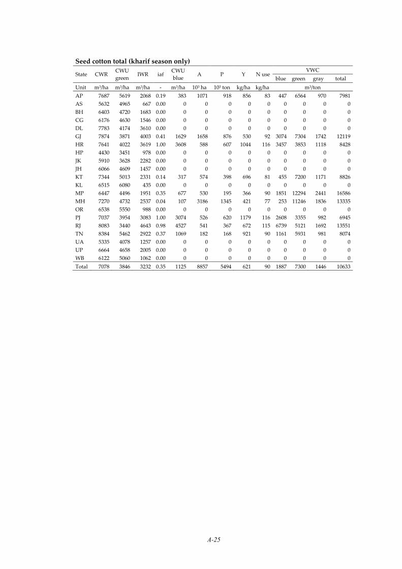
A-25
Seed cotton total (kharif season only)
State CWR CWU
green IWR iaf
CWU
blue A P Y N use
VWC
blue green gray total
Unit m3/ha m3/ha m3/ha - m3/ha 103 ha 103 ton kg/ha kg/ha m3/ton
AP 7687 5619 2068 0.19 383 1071 918 856 83 447 6564 970 7981
AS 5632 4965 667 0.00 0 0 0 0 0 0 0 0 0
BH 6403 4720 1683 0.00 0 0 0 0 0 0 0 0 0
CG 6176 4630 1546 0.00 0 0 0 0 0 0 0 0 0
DL 7783 4174 3610 0.00 0 0 0 0 0 0 0 0 0
GJ 7874 3871 4003 0.41 1629 1658 876 530 92 3074 7304 1742 12119
HR 7641 4022 3619 1.00 3608 588 607 1044 116 3457 3853 1118 8428
HP 4430 3451 978 0.00 0 0 0 0 0 0 0 0 0
JK 5910 3628 2282 0.00 0 0 0 0 0 0 0 0 0
JH 6066 4609 1457 0.00 0 0 0 0 0 0 0 0 0
KT 7344 5013 2331 0.14 317 574 398 696 81 455 7200 1171 8826
KL 6515 6080 435 0.00 0 0 0 0 0 0 0 0 0
MP 6447 4496 1951 0.35 677 530 195 366 90 1851 12294 2441 16586
MH 7270 4732 2537 0.04 107 3186 1345 421 77 253 11246 1836 13335
OR 6538 5550 988 0.00 0 0 0 0 0 0 0 0 0
PJ 7037 3954 3083 1.00 3074 526 620 1179 116 2608 3355 982 6945
RJ 8083 3440 4643 0.98 4527 541 367 672 115 6739 5121 1692 13551
TN 8384 5462 2922 0.37 1069 182 168 921 90 1161 5931 981 8074
UA 5335 4078 1257 0.00 0 0 0 0 0 0 0 0 0
UP 6664 4658 2005 0.00 0 0 0 0 0 0 0 0 0
WB 6122 5060 1062 0.00 0 0 0 0 0 0 0 0 0
Total 7078 3846 3232 0.35 1125 8857 5494 621 90 1887 7300 1446 10633
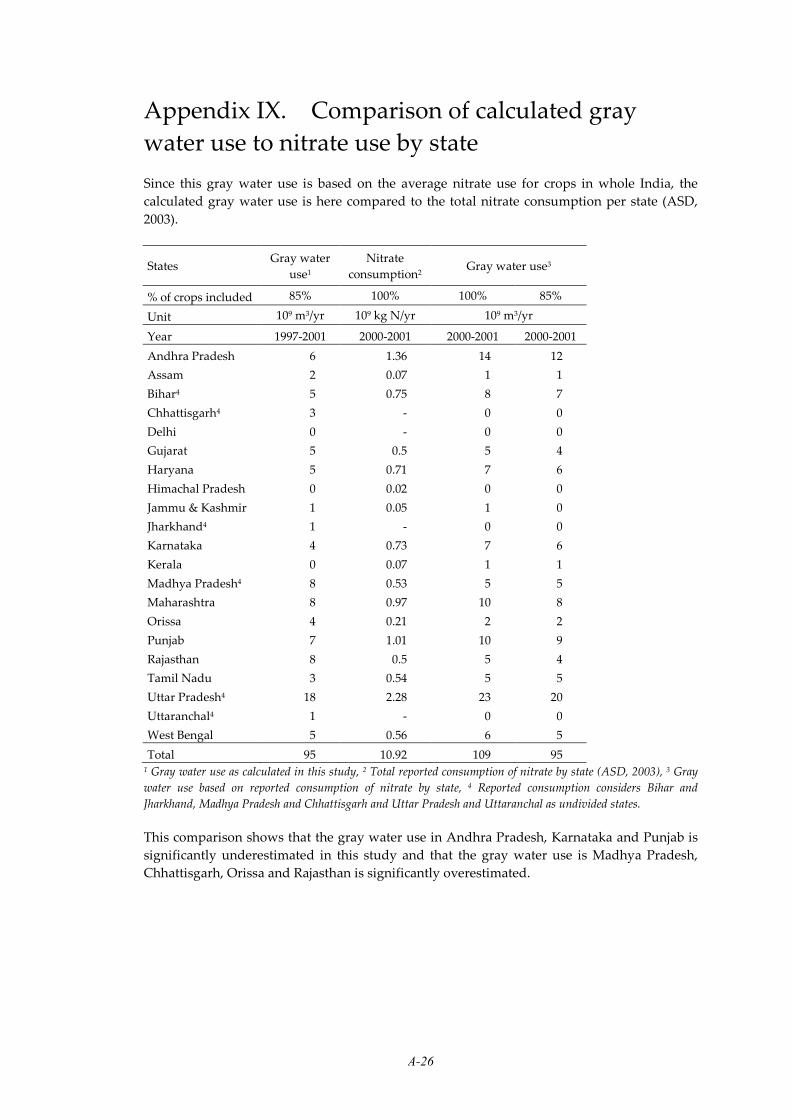
A-26
Appendix IX. Comparison of calculated gray
water use to nitrate use by state
Since this gray water use is based on the average nitrate use for crops in whole India, the
calculated gray water use is here compared to the total nitrate consumption per state (ASD,
2003).
States Gray water
use1
Nitrate
consumption2 Gray water use3
% of crops included 85% 100% 100% 85%
Unit 109 m3/yr 109 kg N/yr 109 m3/yr
Year 1997-2001 2000-2001 2000-2001 2000-2001
Andhra Pradesh 6 1.36 14 12
Assam 2 0.07 1 1
Bihar4 5 0.75 8 7
Chhattisgarh4 3 - 0 0
Delhi 0 - 0 0
Gujarat 5 0.5 5 4
Haryana 5 0.71 7 6
Himachal Pradesh 0 0.02 0 0
Jammu & Kashmir 1 0.05 1 0
Jharkhand4 1 - 0 0
Karnataka 4 0.73 7 6
Kerala 0 0.07 1 1
Madhya Pradesh4 8 0.53 5 5
Maharashtra 8 0.97 10 8
Orissa 4 0.21 2 2
Punjab 7 1.01 10 9
Rajasthan 8 0.5 5 4
Tamil Nadu 3 0.54 5 5
Uttar Pradesh4 18 2.28 23 20
Uttaranchal4 1 - 0 0
West Bengal 5 0.56 6 5
Total 95 10.92 109 95 1 Gray water use as calculated in this study, 2 Total reported consumption of nitrate by state (ASD, 2003), 3 Gray
water use based on reported consumption of nitrate by state, 4 Reported consumption considers Bihar and
Jharkhand, Madhya Pradesh and Chhattisgarh and Uttar Pradesh and Uttaranchal as undivided states.
This comparison shows that the gray water use in Andhra Pradesh, Karnataka and Punjab is
significantly underestimated in this study and that the gray water use is Madhya Pradesh,
Chhattisgarh, Orissa and Rajasthan is significantly overestimated.

A-27
Appendix X. Sensitivity analysis of virtual water
content of kharif milled rice
The divergence in the VWC of the kharif milled rice in the Indian states is in our calculations
quantitatively created by four parameters (see Figure A.1); the crop water requirement of
milled rice in a state, (CWR), the fraction of irrigated area of milled rice in a state (iaf), the
yield of milled rice in a state (Yc) and the use of nitrate in a state (N use). Since the crop
parameters are the same for all Indian states, the CWR is only determined by the average
reference evapotranspiration in a state (ET0). In Figure A.2 the qualitative parameter Crop
variety is added, because normally this parameter has a significant influence on CWR and Yc
and N use.
Figure A.2
Table A.1: Sensitivity analysis VWC kharif milled rice
Parameters R2 Significance
VWC – CWR 0.00175 0.857
VWC – iaf 0.262 0.01757
VWC – Yield* 0.691 0.000003
VWC – N use 0.262 0.01757
Yield – CWR 0.156 0.07679
Yield – iaf* 0.543 0.000140
Yield – N use* 0.543 0.000140
*significant correlation
In Table A.1, it can be seen that there is a significant correlation between the VWC and the
Yield of kharif milled rice. Furthermore there is also a significant correlation between the Yield
and iaf of kharif milled rice. Since the N use is directly based on the iaf, the values of these
parameters are the same.

A-28
Appendix XI. Production, consumption and
surplus of crops
ST/UT Milled rice Wheat Maize Millet
P C Sp P C Sp P C Sp P C Sp
Unit 1000 ton/yr 1000 ton/yr 1000 ton/yr 1000 ton/yr
Year 1997-2001
ANI 29 38 -11 0 7 -7 0 0 0 0 0 0
AP 10935 9818 420 8 330 -324 1446 39 1163 261 312 -73
ARP 129 163 -43 6 15 -10 49 12 29 17 16 -1
AS 3657 3701 -277 100 230 -141 14 0 12 5 0 5
BH 5337 7066 -2070 4508 6396 -2387 1437 758 437 37 0 34
CDG 2 18 -16 0 78 -78 0 1 -1 0 0 0
CG 3835 2891 700 72 271 -207 97 16 64 69 70 -7
DNH 22 17 3 1 5 -5 0 0 0 2 5 -3
DMD 4 13 -9 0 7 -7 0 0 0 0 1 -1
DL 9 295 -287 42 1138 -1100 0 0 0 2 0 2
GOA 155 116 28 0 49 -49 0 0 0 1 0 1
GJ 908 1235 -385 1271 2811 -1680 581 580 -97 1094 1960 -959
HR 2588 194 2229 8653 2523 5173 42 17 18 681 106 517
HP 124 303 -187 530 480 -9 688 265 307 10 10 -1
JK 472 998 -557 352 521 -208 507 224 198 10 8 1
JH 1727 3085 -1469 101 1213 -1124 133 105 5 38 41 -6
KT 3521 3369 -72 198 772 -595 1684 113 1287 1886 1646 80
KL 741 3190 -2497 0 399 -399 0 0 0 3 1 2
LSW 2 7 -5 0 1 -1 0 0 0 0 0 0
MP 1363 1656 -380 7326 5942 573 1312 894 197 312 70 216
MH 2392 3503 -1264 1106 4394 -3411 450 58 315 1391 1483 -210
MNP 372 394 -45 0 4 -4 10 1 8 0 0 0
MGL 167 294 -138 7 7 -1 24 9 11 2 0 2
MIZ 103 124 -27 0 9 -9 15 1 12 0 0 0
NGL 199 315 -129 7 13 -6 46 13 25 8 0 7
OR 5688 5852 -526 8 347 -340 65 7 46 70 190 -126
PDC 58 106 -51 0 7 -7 0 0 0 1 1 0
PJ 8475 235 7700 14462 2694 10168 412 84 259 6 6 -1
RJ 196 174 10 6528 6627 -821 1102 1177 -262 2280 2362 -275
SIK 22 63 -43 12 8 2 53 10 35 5 1 4
TN 7277 6867 -54 0 372 -372 130 3 105 493 379 73
TRP 525 470 22 3 16 -13 2 0 1 0 0 0
UP 11867 7363 3748 23739 17401 3711 1297 545 533 1137 399 641
UA 599 370 191 703 884 -259 49 26 14 270 19 228
WB 13820 10624 2315 867 1433 -662 90 0 75 18 3 13
Total 87317 74929 6823 70609 57404 5393 11735 4956 4793 10123 9091 174
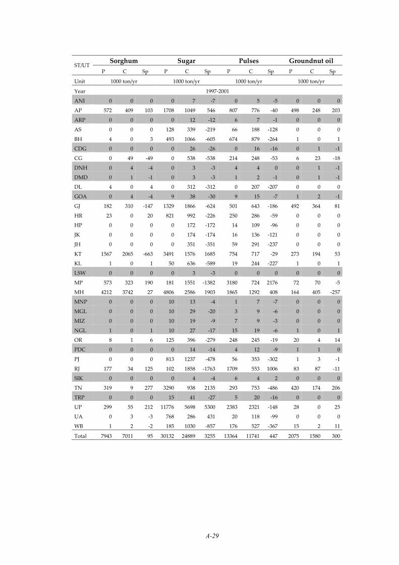
A-29
ST/UT Sorghum Sugar Pulses Groundnut oil
P C Sp P C Sp P C Sp P C Sp
Unit 1000 ton/yr 1000 ton/yr 1000 ton/yr 1000 ton/yr
Year 1997-2001
ANI 0 0 0 0 7 -7 0 5 -5 0 0 0
AP 572 409 103 1708 1049 546 807 776 -40 498 248 203
ARP 0 0 0 0 12 -12 6 7 -1 0 0 0
AS 0 0 0 128 339 -219 66 188 -128 0 0 0
BH 4 0 3 493 1066 -605 674 879 -264 1 0 1
CDG 0 0 0 0 26 -26 0 16 -16 0 1 -1
CG 0 49 -49 0 538 -538 214 248 -53 6 23 -18
DNH 0 4 -4 0 3 -3 4 4 0 0 1 -1
DMD 0 1 -1 0 3 -3 1 2 -1 0 1 -1
DL 4 0 4 0 312 -312 0 207 -207 0 0 0
GOA 0 4 -4 9 38 -30 9 15 -7 1 2 -1
GJ 182 310 -147 1329 1866 -624 501 643 -186 492 364 81
HR 23 0 20 821 992 -226 250 286 -59 0 0 0
HP 0 0 0 0 172 -172 14 109 -96 0 0 0
JK 0 0 0 0 174 -174 16 136 -121 0 0 0
JH 0 0 0 0 351 -351 59 291 -237 0 0 0
KT 1567 2065 -663 3491 1576 1685 754 717 -29 273 194 53
KL 1 0 1 50 636 -589 19 244 -227 1 0 1
LSW 0 0 0 0 3 -3 0 0 0 0 0 0
MP 573 323 190 181 1551 -1382 3180 724 2176 72 70 -5
MH 4212 3742 27 4806 2586 1903 1865 1292 408 164 405 -257
MNP 0 0 0 10 13 -4 1 7 -7 0 0 0
MGL 0 0 0 10 29 -20 3 9 -6 0 0 0
MIZ 0 0 0 10 19 -9 7 9 -3 0 0 0
NGL 1 0 1 10 27 -17 15 19 -6 1 0 1
OR 8 1 6 125 396 -279 248 245 -19 20 4 14
PDC 0 0 0 0 14 -14 4 12 -9 1 1 0
PJ 0 0 0 813 1237 -478 56 353 -302 1 3 -1
RJ 177 34 125 102 1858 -1763 1709 553 1006 83 87 -11
SIK 0 0 0 0 4 -4 6 4 2 0 0 0
TN 319 9 277 3290 938 2135 293 753 -486 420 174 206
TRP 0 0 0 15 41 -27 5 20 -16 0 0 0
UP 299 55 212 11776 5698 5300 2383 2321 -148 28 0 25
UA 0 3 -3 768 286 431 20 118 -99 0 0 0
WB 1 2 -2 185 1030 -857 176 527 -367 15 2 11
Total 7943 7011 95 30132 24889 3255 13364 11741 447 2075 1580 300
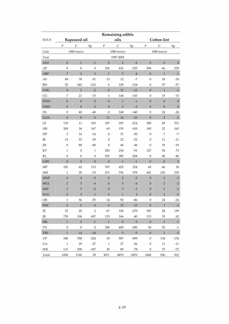
A-30
ST/UT Rapeseed oil
Remaining edible
oils Cotton lint
P C Sp P C Sp P C Sp
Unit 1000 ton/yr 1000 ton/yr 1000 ton/yr
Year 1997-2001
ANI 0 1 -1 0 2 -2 0 0 0
AP 0 0 0 256 416 -255 296 66 229
ARP 7 2 5 1 5 -4 0 1 -1
AS 49 78 -31 13 12 -7 0 18 -18
BH 32 242 -212 6 129 -124 0 57 -57
CDG 0 2 -2 0 12 -12 0 1 -1
CG 7 21 -15 1 144 -143 0 15 -15
DNH 0 0 0 0 1 -1 0 0 0
DMD 0 0 0 0 2 -2 0 0 0
DL 0 40 -40 0 140 -140 0 24 -24
GOA 0 0 0 11 14 -10 0 2 -2
GJ 118 11 103 107 293 -214 380 49 331
HR 209 34 167 65 155 -105 185 22 163
HP 2 16 -14 0 51 -50 0 7 -7
JK 15 53 -39 0 22 -22 0 11 -11
JH 0 80 -80 0 46 -46 0 19 -19
KT 1 0 1 283 218 -51 127 54 73
KL 0 0 0 501 385 -204 0 40 -40
LSW 0 0 0 0 1 -1 0 0 0
MP 181 62 113 767 425 224 65 46 18
MH 1 20 -19 471 756 -378 441 102 339
MNP 0 4 -3 0 2 -2 0 2 -2
MGL 2 5 -4 0 4 -4 0 2 -2
MIZ 1 3 -2 0 3 -3 0 1 -1
NGL 5 3 1 4 1 3 0 2 -2
OR 1 56 -55 14 92 -86 0 24 -24
PDC 0 0 0 0 15 -15 0 1 -1
PJ 23 20 2 67 330 -279 187 28 159
RJ 739 104 607 153 166 -40 115 53 62
SIK 1 2 -1 1 0 0 0 1 -1
TN 0 0 0 308 409 -290 54 55 -1
TRP 1 14 -14 0 5 -5 0 3 -3
UP 348 558 -224 10 507 -499 0 134 -134
UA 1 29 -27 1 27 -26 0 11 -11
WB 115 298 -187 30 89 -78 0 75 -75
Total 1858 1760 29 3071 4879 -2870 1848 926 922
A-31
Appendix XII. Assessment of interstate and
international crop trade
Here, the distribution of the calculated interstate and international crop trade is presented.
The total interstate export Et,is is distributed over the total interstate import It,is. This crop
distribution is based on the assumption that crops are traded as much as possible with
neighbouring states. The first distribution step is to assess the “obvious” trade flows. These
are the flows between adjacent states, when no other states are directly competitive. A second
step can be used for assessing the short distance trade flows that remain after the first step. In
the last step the remaining crop deficits are filled up by the remaining crop surplus.
The international trade of the Indian states is assessed according the part of the national crop
surplus (in the case of international export) or the part of the national crop deficit (in the case
of international import).
Milled rice
The first step is to assess the trade flows between states, when no other states are directly
competitive:
• West Bengal to the North Eastern States (Assam, Arunachal Pradesh, Manipur,
Meghalaya, Mizoram, Nagaland, Sikkim and Tripura). Although West Bengal is not
adjacent to the most of these states, it is still by far the most nearby rice surplus state.
Tripura has a small surplus which goes to Mizoram.
• Uttaranchal to Himachal Pradesh. In this region there are a lot of rice surplus states, so the
surplus goes to the only neighbouring deficit state, which is Himachal Pradesh.
• Chhattisgarh to Madhya Pradesh and Orissa. Because Chhattisgarh was part of Madhya
Pradesh until November 2000, we assume that these trade systems still more or less exist.
The remaining rice surplus of Chhattisgarh goes to Orissa.
• Goa to Karnataka and Rajasthan to Gujarat.
In the second step, the short distance trade flows are assessed that remain after step 1:
• West Bengal to Jharkhand and Orissa. Jharkhand and Orissa receive an equal part of the
remaining rice surplus of West Bengal.
• Andhra Pradesh to Orissa, Karnataka and Tamil Nadu. The small surplus that remains
after filling up these three adjacent states goes to Maharashtra.
• Uttar Pradesh to Bihar and Jharkhand (the latter one was part of Bihar before November
2000). After the first step Uttar Pradesh is only neighbouring state of Bihar and Jharkhand
with a rice surplus. First Jharkhand is filled up, then the remaining surplus goes to Bihar.
• Haryana to Delhi. Because the rice surplus in Uttar Pradesh is all distributed over Bihar
and Jharkhand, the deficit of Delhi is entirely filled up by the rice from Haryana.
In the last step the remaining rice deficits are filled up by the remaining rice surplus in
Haryana and Punjab. These two states are also well known for their function of food grain
supplier to the rest of India. The total of this remaining surplus is 5.72 million ton of rice of
which 1.06 million ton originates from Haryana and 4.66 million ton originates from Punjab.
So all left over deficits are filled with 19% of rice from Haryana and 81% of rice from Punjab.

A-32
Interstate trade of milled rice
ES
IS
Es,
is
Es,
in
AS
BH
DL
GJ
HP
JK
JH
KT
KL
MP
MH
MG
L
NG
L
OR
TN
Unit Million ton/yr
AP 0.1 0.0 0.1 0.1 0.3 0.1
CG 0.4 0.0 0.4 0.1
HR 0.2 0.3 0.1 0.0 0.1 0.5 0.2 1.4 0.3
PJ 0.7 0.3 0.1 0.5 2.0 1.0 4.7 1.2
RJ 0.0 0.0 0.0
UP 1.2 1.1 2.3 0.6
UA 0.1 0.1 0.0
WB 0.3 0.4 0.1 0.1 0.4 1.4 0.3
Is,is 0.3 2.1 0.3 0.4 0.2 0.6 1.5 0.1 2.5 0.4 1.3 0.1 0.1 0.5 0.1 10.5 2.6
Is,in 0.0 0.0 0.0 0.0 0.0 0.0 0.0 0.0 0.0 0.0 0.0 0.0 0.0 0.0 0.0 0.0
Wheat
The first step is to assess the trade flows between states, when no other states are directly
competitive:
• Madhya Pradesh to Chhattisgarh. Because Chhattisgarh was part of Madhya Pradesh
before November 2000, in which we assume that these trade systems still exist. The
remaining part of wheat surplus in Madhya Pradesh goes to Maharashtra.
• Uttar Pradesh to Uttaranchal. Because Uttaranchal was part of Uttar Pradesh before
November 2000, we again assume that these trade systems still exist.
In the second step the remaining wheat deficits are filled up by the remaining wheat surplus
in Haryana, Punjab and Uttar Pradesh. The total of this remaining surplus is 12.65 million ton
of rice of which 3.50 million ton originates from Haryana, 6.88 million ton originates from
Punjab and 2.27 million ton originates from Uttar Pradesh. This means that all the remaining
deficits are filled up with 28% of rice from Haryana, 54% of rice from Punjab and 18% of rice
from Uttar Pradesh.
Interstate trade of wheat
ES IS
Es,
is
Es,
in
AP
AS
BH
CG
DL
GJ
JK
JH
KT
KL
MH
OR
RJ
TN
UA
WB
Unit Million ton/yr
HR 0.1 0.0 0.6 0.3 0.4 0.1 0.3 0.2 0.1 0.8 0.1 0.2 0.1 0.2 3.5 0.2
MP 0.2 0.2 0.4 0.0
PJ 0.2 0.1 1.2 0.6 0.9 0.1 0.6 0.3 0.2 1.6 0.2 0.4 0.2 0.3 6.9 0.4
UP 0.1 0.0 0.4 0.2 0.3 0.0 0.2 0.1 0.1 0.5 0.1 0.1 0.1 0.2 0.1 2.5 0.2
Is,is 0.3 0.1 2.2 0.2 1.0 1.6 0.2 1.0 0.6 0.4 3.2 0.3 0.8 0.3 0.2 0.6 13.3 0.9
Is,in 0.0 0.0 0.2 0.0 0.1 0.1 0.0 0.1 0.0 0.0 0.2 0.0 0.1 0.0 0.0 0.0 0.9

A-33
Maize
The maize deficit in Rajasthan and Gujarat is filled up with maize from Andhra Pradesh and
Karnataka.
Interstate trade of maize
ES IS
Es,
is
Es,
in
GJ
RJ
Unit Million ton./yr
AP 0.1 0.1 0.0
KT 0.1 0.0 0.1 0.0
Is,is 0.1 0.2 0.3 0.1
Is,in 0.0 0.0 0.0
Millet
The first step is to assess the trade flows between states, when no other states are directly
competitive:
• The millet surplus in Tamil Nadu goes to the only neighbouring deficit state Andhra
Pradesh and then the millet surplus of Karnataka goes to the millet deficit Maharashtra.
• The millet deficit in Orissa in filled up by closest millet surplus state Madhya Pradesh.
Then the millet deficit of Maharashtra is filled up by the closest surplus state Madhya
Pradesh, which is not sufficient to fill up the entire millet deficit in Maharashtra.
In the second step the remaining millet deficits are filled up by the remaining millet surplus in
Haryana, Uttar Pradesh and Uttaranchal. The total of this remaining surplus is 1.28 million
ton of millet of which 0.48 million ton originates from Haryana and 0.80 million ton originates
from Uttar Pradesh and Uttaranchal (these two states are linked together because it not clear
whether it comes from Uttar Pradesh or Uttaranchal). This means that all the remaining
deficits are filled up with 38% of millet from Haryana and 62% of millet from Uttar Pradesh
and Uttaranchal.
Interstate trade of millet
IS
Es,
is
ES AP
GJ
MH
OR
RJ
Unit Million ton/yr
HR 0.3 0.0 0.1 0.5
KT 0.0 0.1 0.1
MP 0.1 0.1 0.2
TN 0.1 0.1
UP 0.4 0.0 0.1 0.6
UA 0.2 0.0 0.0 0.2
Is,is 0.1 1.0 0.2 0.1 0.3 1.7

A-34
Sorghum
The first step is to assess the trade flows between states, when no other states are directly
competitive:
• The sorghum surplus of the states Maharashtra, Andhra Pradesh and Tamil Nadu all goes
to the main sorghum deficit state Karnataka.
The remaining deficits in Gujarat and Karnataka are filled up by the remaining surplus, which
is 0.48 million ton (0.15 from Madhya Pradesh, 0.21 from Uttar Pradesh, 0.12 from Rajasthan).
Interstate trade of sorghum
ES
IS
Es,
is
GJ
KT
Unit Million ton/yr
AP 0.1 0.1
MP 0.0 0.1 0.2
RJ 0.1 0.1
TN 0.2 0.2
UP 0.2 0.2
Is,is 0.1 0.7 0.9
Raw sugar
The first step is to assess the trade flows between states, when no other states are directly
competitive:
• Uttar Pradesh and Uttaranchal provide all the Northern states (Punjab, Haryana, Delhi,
Himachal Pradesh, Jammu & Kashmir, Bihar, Jharkhand, West Bengal and all the north
eastern states. Andhra Pradesh, Karnataka, Maharashtra and Tamil Nadu provide
Gujarat, Kerala and Orissa.
The border area in the form of Rajasthan, Madhya Pradesh and Chhattisgarh is filled up with
the remaining surplus of sugar in the exporting states. Most of this comes from the southern
surplus states.
Interstate trade of raw sugar
ES IS
Es,
is
Es,
in
AS
BH
CG
DL
GJ
HR
HP
JK
JH
KL
MP
OR
PJ
RJ
WB
AP 0.1 0.3 0.4 0.0
KT 0.1 1.1 1.2 0.1
MH 0.4 0.6 0.3 1.3 0.1
TN 0.6 0.9 1.5 0.1
UP 0.2 0.5 0.3 0.2 0.1 0.2 0.3 0.4 0.5 0.7 3.7 0.2
UA 0.0 0.0 0.0 0.0 0.0 0.0 0.0 0.0 0.0 0.1 0.3 0.0
Is,is 0.2 0.6 0.5 0.3 0.6 0.2 0.2 0.2 0.3 0.6 1.3 0.3 0.4 1.7 0.8 8.3 0.4
Is,in 0.0 0.0 0.0 0.0 0.0 0.0 0.0 0.0 0.0 0.0 0.1 0.0 0.0 0.1 0.1 0.5
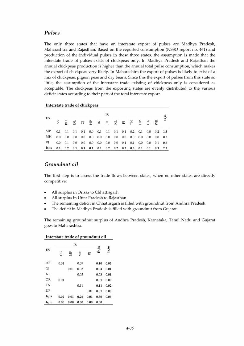
A-35
Pulses
The only three states that have an interstate export of pulses are Madhya Pradesh,
Maharashtra and Rajasthan. Based on the reported consumption (NSSO report no. 461) and
production of the individual pulses in these three states, the assumption is made that the
interstate trade of pulses exists of chickpeas only. In Madhya Pradesh and Rajasthan the
annual chickpeas production is higher than the annual total pulse consumption, which makes
the export of chickpeas very likely. In Maharashtra the export of pulses is likely to exist of a
mix of chickpeas, pigeon peas and dry beans. Since this the export of pulses from this state so
little, the assumption of the interstate trade existing of chickpeas only is considered as
acceptable. The chickpeas from the exporting states are evenly distributed to the various
deficit states according to their part of the total interstate export.
Interstate trade of chickpeas
ES IS
Es,
is
AS
BH
DL
GJ
HP
JK
JH
KL
PJ
TN
UP
UA
WB
MP 0.1 0.1 0.1 0.1 0.0 0.1 0.1 0.1 0.1 0.2 0.1 0.0 0.2 1.3
MH 0.0 0.0 0.0 0.0 0.0 0.0 0.0 0.0 0.0 0.0 0.0 0.0 0.0 0.3
RJ 0.0 0.1 0.0 0.0 0.0 0.0 0.0 0.0 0.1 0.1 0.0 0.0 0.1 0.6
Is,is 0.1 0.2 0.1 0.1 0.1 0.1 0.2 0.2 0.2 0.3 0.1 0.1 0.3 2.2
Groundnut oil
The first step is to assess the trade flows between states, when no other states are directly
competitive:
• All surplus in Orissa to Chhattisgarh
• All surplus in Uttar Pradesh to Rajasthan
• The remaining deficit in Chhattisgarh is filled with groundnut from Andhra Pradesh
• The deficit in Madhya Pradesh is filled with groundnut from Gujarat
The remaining groundnut surplus of Andhra Pradesh, Karnataka, Tamil Nadu and Gujarat
goes to Maharashtra.
Interstate trade of groundnut oil
ES
IS
Es,
is
Es,
in
CG
MP
MH
RJ
AP 0.01 0.09 0.10 0.02
GJ 0.01 0.03 0.04 0.01
KT 0.03 0.03 0.01
OR 0.01 0.01 0.00
TN 0.11 0.11 0.02
UP 0.01 0.01 0.00
Is,is 0.02 0.01 0.26 0.01 0.30 0.06
Is,in 0.00 0.00 0.00 0.00 0.00
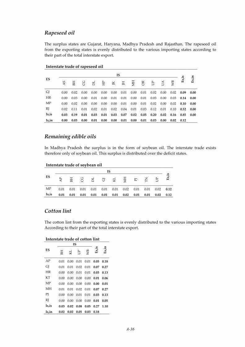
A-36
Rapeseed oil
The surplus states are Gujarat, Haryana, Madhya Pradesh and Rajasthan. The rapeseed oil
from the exporting states is evenly distributed to the various importing states according to
their part of the total interstate export.
Interstate trade of rapeseed oil
ES IS
Es,
is
Es,
in
AS
BH
CG
DL
HP
JK
JH
MH
OR
UP
UA
WB
GJ 0.00 0.02 0.00 0.00 0.00 0.00 0.01 0.00 0.01 0.02 0.00 0.02 0.09 0.00
HR 0.00 0.03 0.00 0.01 0.00 0.01 0.01 0.00 0.01 0.03 0.00 0.03 0.14 0.00
MP 0.00 0.02 0.00 0.00 0.00 0.00 0.01 0.00 0.01 0.02 0.00 0.02 0.10 0.00
RJ 0.02 0.11 0.01 0.02 0.01 0.02 0.04 0.01 0.03 0.12 0.01 0.10 0.52 0.00
Is,is 0.03 0.19 0.01 0.03 0.01 0.03 0.07 0.02 0.05 0.20 0.02 0.16 0.85 0.00
Is,in 0.00 0.03 0.00 0.01 0.00 0.00 0.01 0.00 0.01 0.03 0.00 0.02 0.12
Remaining edible oils
In Madhya Pradesh the surplus is in the form of soybean oil. The interstate trade exists
therefore only of soybean oil. This surplus is distributed over the deficit states.
Interstate trade of soybean oil
ES
IS E
s,is
AP
BH
CG
DL
GJ
KL
MH
PJ
TN
UP
MP 0.01 0.01 0.01 0.01 0.01 0.01 0.02 0.01 0.01 0.02 0.12
Is,is 0.01 0.01 0.01 0.01 0.01 0.01 0.02 0.01 0.01 0.02 0.12
Cotton lint
The cotton lint from the exporting states is evenly distributed to the various importing states
According to their part of the total interstate export.
Interstate trade of cotton lint
ES
IS
Es,
is
Es,
in
BH
KL
UP
WB
AP 0.01 0.00 0.01 0.01 0.05 0.18
GJ 0.01 0.01 0.02 0.01 0.07 0.27
HR 0.00 0.00 0.01 0.01 0.03 0.13
KT 0.00 0.00 0.00 0.00 0.01 0.06
MP 0.00 0.00 0.00 0.00 0.00 0.01
MH 0.01 0.01 0.02 0.01 0.07 0.27
PJ 0.00 0.00 0.01 0.01 0.03 0.13
RJ 0.00 0.00 0.00 0.00 0.01 0.05
Is,is 0.03 0.02 0.08 0.05 0.27 1.10
Is,in 0.02 0.02 0.05 0.03 0.18

A-37
Appendix XIII. Interstate virtual water flows by colour
Gross total virtual water flows
States AP AS BH CG DL GJ HR HP JK JH KT KL MP MH OR PJ RJ TN UP UA WB Export
AP 35 110 481 46 0 0 14 21 36 529 77 0 1814 1051 0 92 190 259 21 144 4952
AS 0 0 0 0 0 0 0 0 0 0 0 0 0 0 0 4 0 0 0 0 4
BH 0 0 1 0 78 0 0 0 0 0 0 0 6 0 0 63 0 0 0 0 149
CG 0 0 0 0 0 0 0 0 0 0 0 2524 0 296 0 15 0 0 0 0 2835
DL 0 0 0 0 0 0 0 0 0 0 0 0 0 0 0 0 0 0 0 0 0
GJ 0 120 530 84 155 0 49 99 188 0 168 87 561 178 0 0 5 874 83 572 3847
HR 80 101 1647 49 1560 2369 86 549 415 148 2098 0 1877 189 0 542 94 478 50 510 13006
HP 0 0 0 0 0 0 0 0 0 0 0 0 0 0 0 26 0 0 0 0 26
JK 0 0 0 0 0 0 0 0 0 0 0 0 0 0 0 26 0 0 0 0 26
JH 0 0 0 0 0 0 0 0 0 0 0 0 0 0 0 0 0 0 0 0 0
KT 19 12 39 10 16 97 0 5 7 13 27 95 663 17 0 1900 1 91 7 51 3130
KL 0 0 0 0 0 0 0 0 0 0 0 0 0 0 0 0 0 0 0 0 0
MP 112 147 470 739 266 312 83 114 150 297 600 273 999 932 348 43 513 518 122 532 7671
MH 11 122 343 873 169 1279 16 60 85 153 85 251 686 121 82 0 137 680 79 455 5788
OR 0 0 0 140 0 0 0 0 0 0 0 0 0 0 0 9 0 0 0 0 149
PJ 124 75 3123 18 450 1542 0 181 1410 453 228 6109 0 4167 159 344 144 156 13 341 19351
RJ 18 289 1620 138 390 1542 27 147 331 674 13 140 0 130 407 138 224 1721 242 1517 9852
TN 128 0 0 0 0 0 0 0 0 0 905 944 1541 738 0 0 15 0 0 0 4293
UP 76 502 6503 9 930 1591 480 371 424 5450 1190 94 0 851 80 1022 2227 88 341 1995 24542
UA 0 31 86 3 44 348 32 411 25 52 0 0 0 27 0 67 182 0 0 121 1447
WB 0 868 0 0 0 28 0 0 0 1122 0 0 0 2 1122 0 15 0 0 0 4447
Import 569 2304 14469 2544 4026 9186 638 1439 3101 8853 3699 10180 4933 11836 4552 1658 5504 1397 4777 960 6238 105516
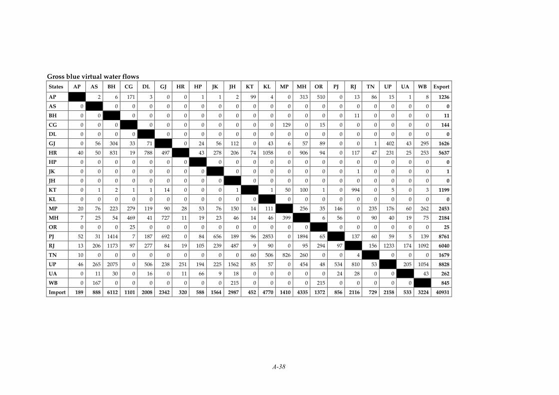
A-38
Gross blue virtual water flows
States AP AS BH CG DL GJ HR HP JK JH KT KL MP MH OR PJ RJ TN UP UA WB Export
AP 2 6 171 3 0 0 1 1 2 99 4 0 313 510 0 13 86 15 1 8 1236
AS 0 0 0 0 0 0 0 0 0 0 0 0 0 0 0 0 0 0 0 0 0
BH 0 0 0 0 0 0 0 0 0 0 0 0 0 0 0 11 0 0 0 0 11
CG 0 0 0 0 0 0 0 0 0 0 0 129 0 15 0 0 0 0 0 0 144
DL 0 0 0 0 0 0 0 0 0 0 0 0 0 0 0 0 0 0 0 0 0
GJ 0 56 304 33 71 0 24 56 112 0 43 6 57 89 0 0 1 402 43 295 1626
HR 40 50 831 19 788 497 43 278 206 74 1058 0 906 94 0 117 47 231 25 253 5637
HP 0 0 0 0 0 0 0 0 0 0 0 0 0 0 0 0 0 0 0 0 0
JK 0 0 0 0 0 0 0 0 0 0 0 0 0 0 0 1 0 0 0 0 1
JH 0 0 0 0 0 0 0 0 0 0 0 0 0 0 0 0 0 0 0 0 0
KT 0 1 2 1 1 14 0 0 0 1 1 50 100 1 0 994 0 5 0 3 1199
KL 0 0 0 0 0 0 0 0 0 0 0 0 0 0 0 0 0 0 0 0 0
MP 20 76 223 279 119 90 28 53 76 150 14 111 256 35 146 0 235 176 60 262 2453
MH 7 25 54 469 41 727 11 19 23 46 14 46 399 6 56 0 90 40 19 75 2184
OR 0 0 0 25 0 0 0 0 0 0 0 0 0 0 0 0 0 0 0 0 25
PJ 52 31 1414 7 187 692 0 84 656 189 96 2853 0 1894 65 137 60 59 5 139 8761
RJ 13 206 1173 97 277 84 19 105 239 487 9 90 0 95 294 97 156 1233 174 1092 6040
TN 10 0 0 0 0 0 0 0 0 0 60 506 826 260 0 0 4 0 0 0 1679
UP 46 265 2075 0 506 238 251 194 225 1562 85 57 0 454 48 534 810 53 205 1054 8828
UA 0 11 30 0 16 0 11 66 9 18 0 0 0 0 0 24 28 0 0 43 262
WB 0 167 0 0 0 0 0 0 0 215 0 0 0 0 215 0 0 0 0 0 845
Import 189 888 6112 1101 2008 2342 320 588 1564 2987 452 4770 1410 4335 1372 856 2116 729 2158 533 3224 40931
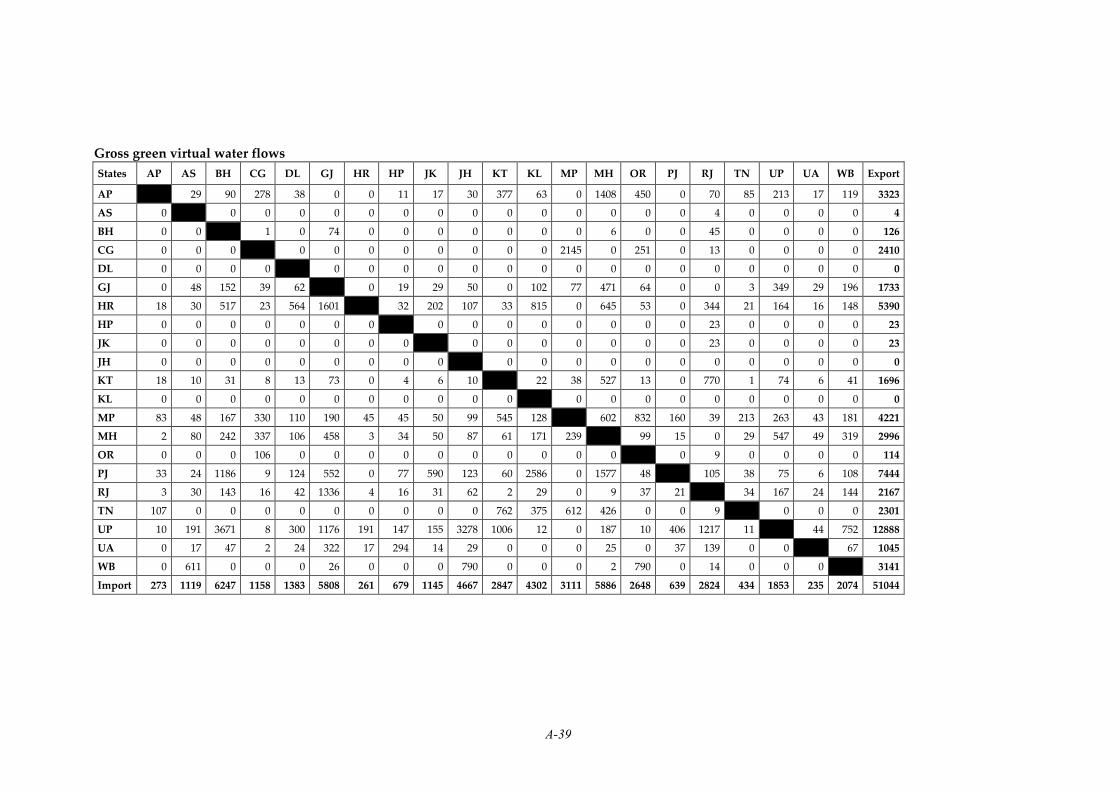
A-39
Gross green virtual water flows
States AP AS BH CG DL GJ HR HP JK JH KT KL MP MH OR PJ RJ TN UP UA WB Export
AP 29 90 278 38 0 0 11 17 30 377 63 0 1408 450 0 70 85 213 17 119 3323
AS 0 0 0 0 0 0 0 0 0 0 0 0 0 0 0 4 0 0 0 0 4
BH 0 0 1 0 74 0 0 0 0 0 0 0 6 0 0 45 0 0 0 0 126
CG 0 0 0 0 0 0 0 0 0 0 0 2145 0 251 0 13 0 0 0 0 2410
DL 0 0 0 0 0 0 0 0 0 0 0 0 0 0 0 0 0 0 0 0 0
GJ 0 48 152 39 62 0 19 29 50 0 102 77 471 64 0 0 3 349 29 196 1733
HR 18 30 517 23 564 1601 32 202 107 33 815 0 645 53 0 344 21 164 16 148 5390
HP 0 0 0 0 0 0 0 0 0 0 0 0 0 0 0 23 0 0 0 0 23
JK 0 0 0 0 0 0 0 0 0 0 0 0 0 0 0 23 0 0 0 0 23
JH 0 0 0 0 0 0 0 0 0 0 0 0 0 0 0 0 0 0 0 0 0
KT 18 10 31 8 13 73 0 4 6 10 22 38 527 13 0 770 1 74 6 41 1696
KL 0 0 0 0 0 0 0 0 0 0 0 0 0 0 0 0 0 0 0 0 0
MP 83 48 167 330 110 190 45 45 50 99 545 128 602 832 160 39 213 263 43 181 4221
MH 2 80 242 337 106 458 3 34 50 87 61 171 239 99 15 0 29 547 49 319 2996
OR 0 0 0 106 0 0 0 0 0 0 0 0 0 0 0 9 0 0 0 0 114
PJ 33 24 1186 9 124 552 0 77 590 123 60 2586 0 1577 48 105 38 75 6 108 7444
RJ 3 30 143 16 42 1336 4 16 31 62 2 29 0 9 37 21 34 167 24 144 2167
TN 107 0 0 0 0 0 0 0 0 0 762 375 612 426 0 0 9 0 0 0 2301
UP 10 191 3671 8 300 1176 191 147 155 3278 1006 12 0 187 10 406 1217 11 44 752 12888
UA 0 17 47 2 24 322 17 294 14 29 0 0 0 25 0 37 139 0 0 67 1045
WB 0 611 0 0 0 26 0 0 0 790 0 0 0 2 790 0 14 0 0 0 3141
Import 273 1119 6247 1158 1383 5808 261 679 1145 4667 2847 4302 3111 5886 2648 639 2824 434 1853 235 2074 51044

A-40
Gross gray virtual water flows
States AP AS BH CG DL GJ HR HP JK JH KT KL MP MH OR PJ RJ TN UP UA WB Export
AP 4 13 31 6 0 0 2 3 4 53 9 0 92 91 0 9 20 32 3 18 393
AS 0 0 0 0 0 0 0 0 0 0 0 0 0 0 0 0 0 0 0 0 0
BH 0 0 0 0 4 0 0 0 0 0 0 0 0 0 0 6 0 0 0 0 11
CG 0 0 0 0 0 0 0 0 0 0 0 251 0 29 0 1 0 0 0 0 282
DL 0 0 0 0 0 0 0 0 0 0 0 0 0 0 0 0 0 0 0 0 0
GJ 0 17 74 12 22 0 7 14 26 0 24 5 34 25 0 0 1 123 12 80 488
HR 22 21 298 7 208 271 11 69 102 41 225 0 326 42 0 81 26 84 9 108 1980
HP 0 0 0 0 0 0 0 0 0 0 0 0 0 0 0 3 0 0 0 0 3
JK 0 0 0 0 0 0 0 0 0 0 0 0 0 0 0 3 0 0 0 0 3
JH 0 0 0 0 0 0 0 0 0 0 0 0 0 0 0 0 0 0 0 0 0
KT 1 2 5 1 2 10 0 1 1 2 4 7 37 2 0 136 0 12 1 7 235
KL 0 0 0 0 0 0 0 0 0 0 0 0 0 0 0 0 0 0 0 0 0
MP 9 23 80 130 37 32 9 16 24 47 40 33 140 65 42 3 65 79 19 88 998
MH 1 17 47 67 23 94 2 8 11 21 10 34 48 17 11 0 18 93 11 62 608
OR 0 0 0 9 0 0 0 0 0 0 0 0 0 0 0 1 0 0 0 0 10
PJ 40 20 523 2 138 299 0 20 164 140 73 670 0 697 46 103 46 22 2 93 3146
RJ 3 52 304 25 70 122 4 26 61 125 2 20 0 25 77 21 35 321 44 282 1645
TN 11 0 0 0 0 0 0 0 0 0 83 63 102 52 0 0 2 0 0 0 313
UP 21 47 757 1 124 177 38 30 43 609 99 26 0 210 22 82 200 24 92 190 2825
UA 0 3 8 0 4 26 3 52 2 5 0 0 0 2 0 6 15 0 0 12 141
WB 0 90 0 0 0 2 0 0 0 117 0 0 0 0 117 0 1 0 0 0 461
Import 108 296 2111 286 635 1035 57 172 392 1198 401 1108 413 1615 532 163 565 234 766 192 939 13541

A-41
Net total virtual water flows
States AP AS BH CG DL GJ HR HP JK JH KT KL MP MH OR PJ RJ TN UP UA WB Export
AP 35 110 481 46 0 -80 14 21 36 510 77 -112 1803 1051 -124 73 62 183 21 144 4383
AS -35 0 0 0 -120 -101 0 0 0 -12 0 -147 -122 0 -75 -285 0 -502 -31 -868 -2300
BH -110 0 1 0 -451 -1647 0 0 0 -39 0 -470 -336 0 -3123 -1557 0 -6503 -86 0 -14321
CG -481 0 -1 0 -84 -49 0 0 0 -10 0 1785 -873 156 -18 -123 0 -9 -3 0 291
DL -46 0 0 0 -155 -1560 0 0 0 -16 0 -266 -169 0 -450 -390 0 -930 -44 0 -4026
GJ 0 120 451 84 155 -2369 49 99 188 -97 168 -225 -717 178 -1542 -1542 5 -717 -264 544 -5339
HR 80 101 1647 49 1560 2369 86 549 415 148 2098 -83 1861 189 0 515 94 -3 19 510 12368
HP -14 0 0 0 0 -49 -86 0 0 -5 0 -114 -60 0 -181 -121 0 -371 -411 0 -1414
JK -21 0 0 0 0 -99 -549 0 0 -7 0 -150 -85 0 -1410 -305 0 -424 -25 0 -3075
JH -36 0 0 0 0 -188 -415 0 0 -13 0 -297 -153 0 -453 -674 0 -5450 -52 -1122 -8853
KT -510 12 39 10 16 97 -148 5 7 13 27 -505 578 17 -228 1887 -904 -1099 7 51 -569
KL -77 0 0 0 0 -168 -2098 0 0 0 -27 -273 -251 0 -6109 -140 -944 -94 0 0 -10180
MP 112 147 470 -1785 266 225 83 114 150 297 505 273 313 932 348 43 -1027 518 122 532 2738
MH -1803 122 336 873 169 717 -1861 60 85 153 -578 251 -313 121 -4086 -130 -601 -171 52 453 -6048
OR -1051 0 0 -156 0 -178 -189 0 0 0 -17 0 -932 -121 -159 -398 0 -80 0 -1122 -4403
PJ 124 75 3123 18 450 1542 0 181 1410 453 228 6109 -348 4086 159 206 144 -866 -55 341 17694
RJ -73 285 1557 123 390 1542 -515 121 305 674 -1887 140 -43 130 398 -206 209 -506 60 1502 4348
TN -62 0 0 0 0 -5 -94 0 0 0 904 944 1027 601 0 -144 -209 -88 0 0 2897
UP -183 502 6503 9 930 717 3 371 424 5450 1099 94 -518 171 80 866 506 88 341 1995 19765
UA -21 31 86 3 44 264 -19 411 25 52 -7 0 -122 -52 0 55 -60 0 -341 121 487
WB -144 868 0 0 0 -544 -510 0 0 1122 -51 0 -532 -453 1122 -341 -1502 0 -1995 -121 -1791
Import -4383 2300 14321 -291 4026 5339 -12368 1414 3075 8853 569 10180 -2738 6048 4403 -17694 -4348 -2897 -19765 -487 1791

A-42
Appendix XIV. Water footprints by colour
Blue water footprints of the consumption of agricultural commodities
State Blue state water footprint Blue water footprint per capita
Internal External Total Internal External Total
Unit 109 m3/yr m3/cap/yr
Year 1997-2001
Andhra Pradesh 20 1 21 273 13 286
Assam 0 1 2 18 40 58
Bihar 9 7 16 110 88 198
Chhattisgarh 1 2 3 63 82 144
Delhi 0 3 3 9 200 209
Gujarat 10 3 13 199 66 266
Haryana 8 1 9 390 32 422
Himachal Pradesh 0 1 1 11 135 147
Jammu & Kashmir 1 2 3 91 177 267
Jharkhand 1 3 4 35 130 166
Karnataka 9 1 10 180 13 193
Kerala 0 6 6 11 183 194
Madhya Pradesh 12 2 13 201 27 228
Maharashtra 12 6 17 123 62 184
Orissa 3 2 5 83 50 133
Punjab 9 2 10 362 76 438
Rajasthan 15 3 18 274 47 321
Tamil Nadu 13 2 14 207 28 235
Uttar Pradesh 39 4 43 243 25 269
Uttaranchal 1 1 2 103 84 188
West Bengal 9 4 13 116 52 168
Total 172 55 227 172 55 227
Green water footprints of the consumption of agricultural commodities
State Green state water footprint Green water footprint per capita
Internal External Total Internal External Total
Unit 109 m3/yr m3/cap/yr
Year 1997-2001
Andhra Pradesh 34 0 34 458 4 462
Assam 16 1 17 601 43 644
Bihar 24 6 30 296 77 374
Chhattisgarh 21 1 22 1020 57 1078
Delhi 0 1 1 7 103 110
Gujarat 22 6 28 453 116 569
Haryana 6 0 6 303 13 316
Himachal Pradesh 2 1 3 320 115 434
Jammu & Kashmir 3 1 4 263 116 379
Jharkhand 9 5 14 360 178 538
Karnataka 27 3 30 519 55 575
Kerala 2 4 7 73 139 212
Madhya Pradesh 30 3 33 516 53 569
Maharashtra 52 6 58 553 62 615
Orissa 31 3 34 869 74 943
Punjab 8 1 9 326 42 368
Rajasthan 29 2 31 528 45 573
Tamil Nadu 15 0 16 255 7 262
Uttar Pradesh 46 2 48 283 11 294
Uttaranchal 2 0 3 297 28 326
West Bengal 28 3 30 358 33 390
Total 407 52 459 407 52 459

A-43
Gray water footprints of the consumption of agricultural commodities
State Gray state water footprint Gray water footprint per capita
Internal External Total Internal External Total
Unit 109 m3/yr m3/cap/yr
Year 1997-2001
Andhra Pradesh 6 0 6 78 1 79
Assam 2 0 2 68 11 80
Bihar 5 2 7 66 26 92
Chhattisgarh 2 0 3 120 14 134
Delhi 0 1 1 3 47 50
Gujarat 4 1 5 74 21 95
Haryana 3 0 3 127 3 130
Himachal Pradesh 0 0 1 73 29 102
Jammu & Kashmir 1 0 1 62 40 101
Jharkhand 1 1 2 47 46 93
Karnataka 4 0 4 74 8 82
Kerala 0 1 1 10 36 46
Madhya Pradesh 7 0 7 116 7 123
Maharashtra 7 2 9 74 17 91
Orissa 4 1 4 99 15 114
Punjab 3 0 3 138 9 146
Rajasthan 6 1 7 111 10 121
Tamil Nadu 3 0 3 48 4 51
Uttar Pradesh 15 1 16 94 5 99
Uttaranchal 1 0 1 85 23 108
West Bengal 5 1 6 60 13 73
Total 78 14 92 78 14 92
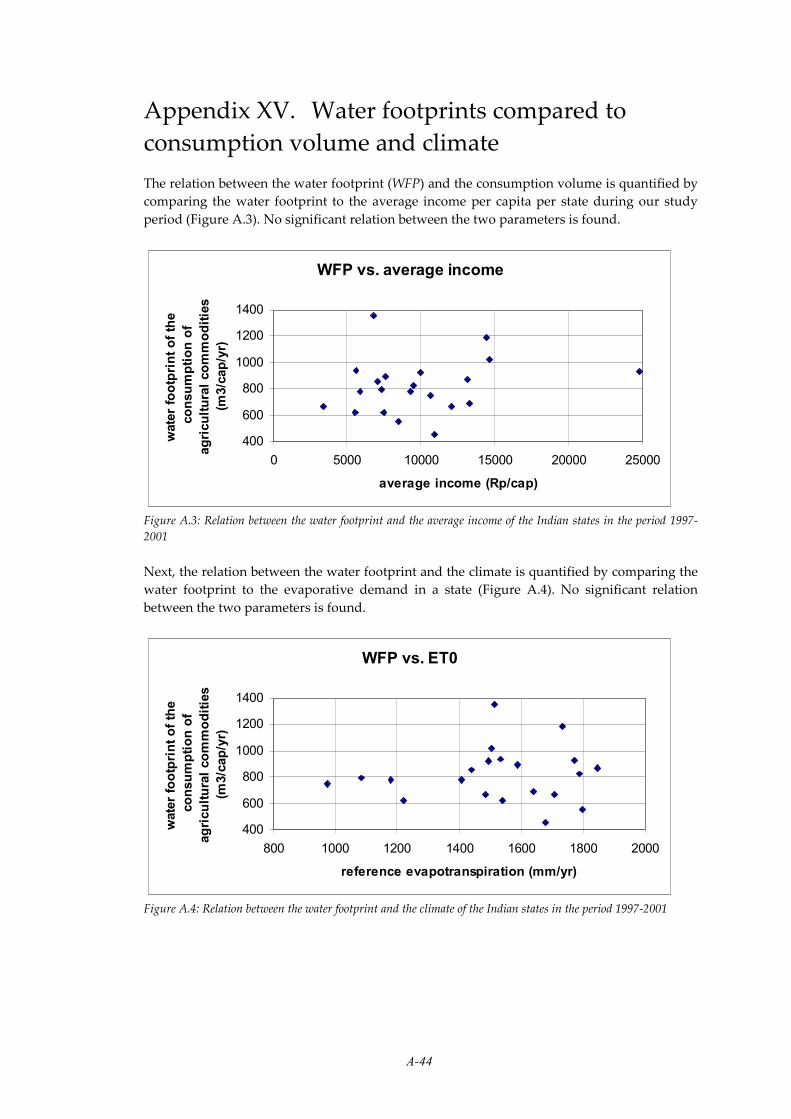
A-44
Appendix XV. Water footprints compared to
consumption volume and climate
The relation between the water footprint (WFP) and the consumption volume is quantified by
comparing the water footprint to the average income per capita per state during our study
period (Figure A.3). No significant relation between the two parameters is found.
WFP vs. average income
400
600
800
1000
1200
1400
0 5000 10000 15000 20000 25000
average income (Rp/cap)
water footprint of the
consumption of
agricultural commodities
(m3/cap/yr)
Figure A.3: Relation between the water footprint and the average income of the Indian states in the period 1997-
2001
Next, the relation between the water footprint and the climate is quantified by comparing the
water footprint to the evaporative demand in a state (Figure A.4). No significant relation
between the two parameters is found.
WFP vs. ET0
400
600
800
1000
1200
1400
800 1000 1200 1400 1600 1800 2000
reference evapotranspiration (mm/yr)
water footprint of the
consumption of
agricultural commodities
(m3/cap/yr)
Figure A.4: Relation between the water footprint and the climate of the Indian states in the period 1997-2001

A-45
Appendix XVI. Other estimates on the water
resources of India
Many studies have been executed to estimate the total water resources of India. The outcome
of three important studies is presented here to create a reference for calculations in this study.
FAO (2006e)
A simplified hydrological concept is used in the computation of the total internal renewable
water resources. The input is the total precipitation, which results either in evapotranspiration
(runoff deficit), infiltration and groundwater recharge (in the aquifers) or direct surface runoff
(in the rivers). In this concept an estimate is made for the overlap between aquifers and rivers.
This overlap represents that part of the water resources that belongs to rivers as well as
aquifers (FAO, 2003). FAO presents the following data on the total water resources of India:
• Precipitation = 1083 mm x 328.726.000 ha = 3559 km3/year
• Internally produced surface water = 1869 (outflow) – 636 (inflow) = 1233 km3/year
• Internally produced groundwater = 419 km3/year
• Overlap of surface and groundwater = 380 km3/year
• Total internal renewable water resources = 1233 + 419 – 380 = 1272 km3/year
• Total renewable water resources = 1272 + 636 = 1908 km3/year
• Runoff deficit (Precipitation - IRWR) = 3559 – 1272 = 2287 km3/year
Ministry of Water Resources (2006a)
In this assessment of (blue) water resources of the various river basins, the vapour flows are
excluded and the inflow of surface water is not separated from internally produced surface
water. Therefore the water balance is not complete. The Ministry of Water Resources presents
the following data on the total water resources of India:
• Precipitation = 4000 km3/year
• Internally and externally produced surface water = 1869 km3/year
• Internally produced groundwater = 432 km3/year
• Overlap of surface water and groundwater = not estimated
Chaturvedi (1985)
In 1974, the National Commission on Agriculture estimated the national water balance of
India for the years 1974, 2000 and 2025 (Chaturvedi, 1985). In this calculation the average
annual rainfall is assessed at 3940 km3 (1194 mm). This is rounded off to 4000 km3 since
snowfall is not yet included. Chaturvedi (1985) presents the following data on the total water
resources of India:
• Precipitation (including snowfall) = 4000 km3/year
• Immediate evapotranspiration from soil = 700 km3/year
• Infiltration to soil moisture = 1650 km3/year
• Percolation to groundwater = 500 km3/year
• Surface runoff to surface water = 1150 km3/year
• Net flow from groundwater to surface water = 350 km3/year
• Runoff deficit = soil moisture + evapotranspiration = 2350 km3/year
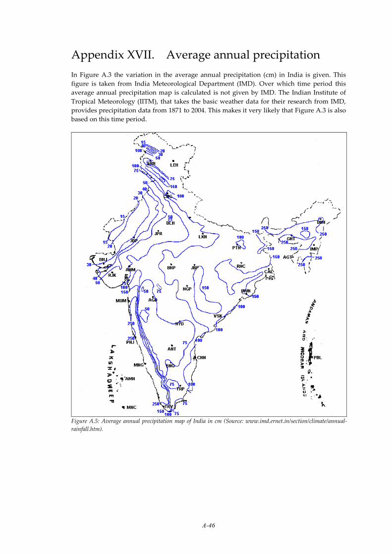
A-46
Appendix XVII. Average annual precipitation
In Figure A.3 the variation in the average annual precipitation (cm) in India is given. This
figure is taken from India Meteorological Department (IMD). Over which time period this
average annual precipitation map is calculated is not given by IMD. The Indian Institute of
Tropical Meteorology (IITM), that takes the basic weather data for their research from IMD,
provides precipitation data from 1871 to 2004. This makes it very likely that Figure A.3 is also
based on this time period.
Figure A.5: Average annual precipitation map of India in cm (Source: www.imd.ernet.in/section/climate/annual-
rainfall.htm).

A-47
Appendix XVIII. Water resources of the Indian
states
States
Total water resources Water resources by capita
Green Blue
Green Blue
Internal External Total Internal External Total
unit billion m3/yr m3/cap/yr
year 1997-2001
Andhra Pradesh 188 66 206 272 2537 896 2774 3670
Assam 75 103 567 670 2912 3965 21879 25844
Bihar 64 51 442 493 789 628 5482 6109
Chhattisgarh 91 105 9 114 4496 5174 452 5626
Delhi 1 0 0 0 58 18 0 18
Gujarat 88 47 92 139 1789 961 1860 2821
Haryana 23 8 14 22 1121 391 663 1055
Himachal Pradesh 39 50 11 62 6553 8496 1934 10430
Jammu & Kashmir 104 37 13 49 10577 3712 1291 5004
Jharkhand 55 52 14 65 2082 1970 528 2498
Karnataka 140 113 31 144 2733 2199 612 2811
Kerala 39 65 0 65 1255 2112 0 2112
Madhya Pradesh 170 193 0 193 2898 3289 0 3289
Maharashtra 179 132 19 151 1896 1404 204 1608
Orissa 123 110 78 188 3446 3079 2185 5264
Punjab 26 5 54 58 1102 193 2260 2452
Rajasthan 128 42 4 46 2334 765 71 835
Tamil Nadu 93 34 25 60 1525 568 417 985
Uttar Pradesh 139 93 240 333 863 575 1485 2059
Uttaranchal 36 50 0 50 4347 6045 0 6045
West Bengal 74 76 537 613 945 978 6885 7864
INDIA Total 2048 1705 636 2341 2053 1709 638 2347
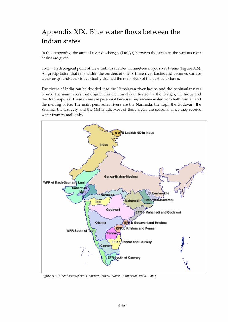
A-48
Appendix XIX. Blue water flows between the
Indian states
In this Appendix, the annual river discharges (km3/yr) between the states in the various river
basins are given.
From a hydrological point of view India is divided in nineteen major river basins (Figure A.6).
All precipitation that falls within the borders of one of these river basins and becomes surface
water or groundwater is eventually drained the main river of the particular basin.
The rivers of India can be divided into the Himalayan river basins and the peninsular river
basins. The main rivers that originate in the Himalayan Range are the Ganges, the Indus and
the Brahmaputra. These rivers are perennial because they receive water from both rainfall and
the melting of ice. The main peninsular rivers are the Narmada, the Tapi, the Godavari, the
Krishna, the Cauvery and the Mahanadi. Most of these rivers are seasonal since they receive
water from rainfall only.
Figure A.6: River basins of India (source: Central Water Commission India, 2006).

A-49
Main channel
Tributary/bifurcation
Indian State
Country
Sea/ocean
Ganges River Basin (557 km3/year)
Uttaranchal(49)
Nepal(210)
Uttar Pradesh(44)
Haryana(-5)
Rajasthan(7)
Madhya Pradesh
(106)
Bihar(42) West
Bengal(55)
Bangladesh / Bay of Bengal
4
13
106
Jharkhand(32)
Himachal Pradesh
(4)
Chhattisgarh(13)
39 80 130
285
486
55729
9
Annual average discharge in km3 / year
Brahmaputra River Basin (677 km3/year) China(327)
Arunachal Pradesh(114)
Assam(92)
Bangladesh
Bhutan(90)
Sikkim(12)
West Bengal(10)
Meghalaya(22)
Nagaland(11)
327
4417512
37 641 22
11
15
Barak River Basin (63 km3/year) Meghalaya(20)
Assam(10)
Manipur(10)
BangladeshTripura
(15)Mizoram
(9)15
20 28
10
9
N
EW
S
16
10
7

A-50
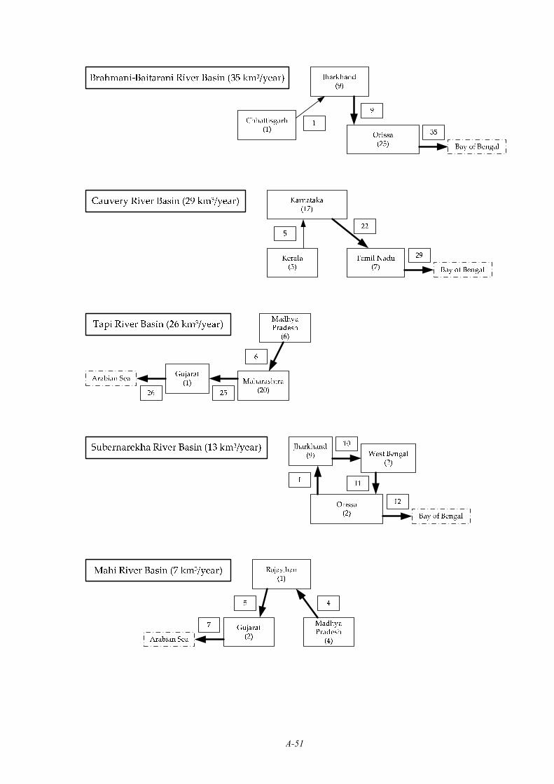
A-51

A-52
Pennar River Basin (11 km3/year)
Karnataka(3)
Andhra Pradesh(8)
Bay of Bengal
311
Sabarmati River Basin (3 km3/year) Rajasthan(0)
Gujarat(3)
Arabian Sea
0
3
Rajasthan(11)
Gujarat(26)
Arabian Sea
11
36
Luni River Basin and the river basins of Saurashtra (36 km3/year)
East flowing river basins between Pennar River and Kanyakumari (18 km3/year)
Karnataka(3)
Tamil Nadu(13)3 16
Bay of Bengal
River basins which do not cross state borders:
- West flowing river basins between Tapi River and Kanyakumari- East flowing river basins between Mahanadi River and Pennar River- North eastern river basins flowing into Myanmar
Andhra Pradesh(2)
2

A-53
Areas of states in
river basins
(km2) R
iver
s
Gan
ges
Bra
hm
ap
utr
a
Bar
ak-
Meg
hn
a
Wes
t T
adri
-
Kan
ya
ku
mar
i
Go
dav
ari
Wes
t T
api-
Tad
ri
Kri
shn
a
Ind
us
Mah
anad
i
Nar
ma
da
No
rth
east
ern
riv
ers
Bra
hm
ani-
Bai
tara
ni
Eas
t
Mah
anad
i-
Pen
nar
Cau
ver
y
Eas
t P
enn
ar-
Kan
ya
ku
mar
i
Ku
tch
-
Sau
rash
tra
Tap
i
Su
ber
nar
ak
ha
Mah
i
Pen
nar
Sab
arm
ati
Raj
asth
an
inla
nd
bas
in
State Area 861452 194413 41723 56177 312812 55940 258948 321289 141589 98796 36302 51822 86600 81155 100139 321851 65145 19296 34842 55213 21674 14000
Andhra Pradesh 275068 0 0 0 0 73201 0 76251 0 0 0 0 0 66669 0 10671 0 0 0 0 48276 0 0
Arunachal Pradesh 83743 0 81616 0 0 0 0 0 0 0 0 0 0 0 0 0 0 0 0 0 0 0 0
Assam 78483 0 70800 7683 0 0 0 0 0 0 0 0 0 0 0 0 0 0 0 0 0 0 0
Bihar 94164 94164 0 0 0 0 0 0 0 0 0 0 0 0 0 0 0 0 0 0 0 0 0
Chhattisgarh 135194 16758 0 0 0 41867 0 0 0 74982 170 0 1316 0 0 0 0 0 0 0 0 0 0
Delhi 1483 1483 0 0 0 0 0 0 0 0 0 0 0 0 0 0 0 0 0 0 0 0 0
Goa 3702 0 0 0 0 0 3702 0 0 0 0 0 0 0 0 0 0 0 0 0 0 0 0
Gujarat 196024 0 0 0 0 0 9000 0 0 0 11399 0 0 0 0 0 142544 3837 0 11694 0 17550 0
Haryana 44212 34341 0 0 0 0 0 0 9939 0 0 0 0 0 0 0 0 0 0 0 0 0 0
Himachal Pradesh 55673 4317 0 0 0 0 0 0 51356 0 0 0 0 0 0 0 0 0 0 0 0 0 0
Jammu & Kashmir 222236 0 0 0 0 0 0 0 193762 0 0 0 0 0 0 0 0 0 0 0 0 0 0
Jharkhand 79700 49797 0 0 0 0 0 0 0 635 0 0 14508 0 0 0 0 0 14093 0 0 0 0
Karnataka 191791 0 0 0 16600 4405 9790 113272 0 0 0 0 0 0 34273 6514 0 0 0 0 6937 0 0
Kerala 38863 0 0 0 35997 0 0 0 0 0 0 0 0 0 2866 0 0 0 0 0 0 0 0
Madhya Pradesh 308144 182204 0 0 0 23388 0 0 0 154 85689 0 0 0 0 0 0 9804 0 6695 0 0 0
Maharashtra 307713 0 0 0 0 152199 32809 69425 0 238 1538 0 0 0 0 0 0 51504 0 0 0 0 0
Manipur 22327 0 0 7442 0 0 0 0 0 0 0 14885 0 0 0 0 0 0 0 0 0 0 0
Meghalaya 22429 0 11888 10541 0 0 0 0 0 0 0 0 0 0 0 0 0 0 0 0 0 0 0
Mizoram 21081 0 0 5270 0 0 0 0 0 0 0 15811 0 0 0 0 0 0 0 0 0 0 0
Nagaland 16579 0 10855 0 0 0 0 0 0 0 0 5724 0 0 0 0 0 0 0 0 0 0 0
Orissa 155707 0 0 0 0 17752 0 0 0 65580 0 0 35998 33398 0 0 0 0 2983 0 0 0 0
Punjab 50362 0 0 0 0 0 0 0 50304 0 0 0 0 0 0 0 0 0 0 0 0 0 0
Rajasthan 342236 112490 0 0 0 0 0 0 15814 0 0 0 0 0 0 0 179307 0 0 16453 0 4124 14000
Sikkim 7096 0 7096 0 0 0 0 0 0 0 0 0 0 0 0 0 0 0 0 0 0 0 0
Tamil Nadu 130058 0 0 0 3580 0 0 0 0 0 0 0 0 0 43868 82610 0 0 0 0 0 0 0
Tripura 10492 0 0 10492 0 0 0 0 0 0 0 0 0 0 0 0 0 0 0 0 0 0 0
Uttar Pradesh 238566 238566 0 0 0 0 0 0 0 0 0 0 0 0 0 0 0 0 0 0 0 0 0
Uttaranchal 53566 53566 0 0 0 0 0 0 0 0 0 0 0 0 0 0 0 0 0 0 0 0 0
West Bengal 88752 73766 12758 0 0 0 0 0 0 0 0 0 0 0 0 0 0 2220 0 0 0 0

A-54
Appendix XX. Assessment of water scarcity in a
potential situation
Here the calculation of the water scarcity from production and consumption perspective is
presented for the potential situation of increased water productivity combined with the
omission of the interstate trade in milled rice from Punjab and Uttar Pradesh to Bihar (see
Table 7.7 in Chapter 7.3.2).
Water scarcity in the potential situation from a production perspective
From Table 7.4 and Table 7.5, the water saving as a result of the shift from the current
situation to the potential situation can be calculated by colour and by state. The total water
use is presented by colour and by state in Table 6.1. In Table A.2, the total agricultural water
use is presented for the current and potential situation.
Table A.2: Agricultural water use in the current and potential situation in Bihar, Punjab and Uttar
Pradesh in the period 1997-2001
States Total agricultural water use in current
situation
Total agricultural water use in potential
situation
Blue + Gray Green Total Blue + Gray Green Total
Unit 109 m3/yr
Bihar 14 24 38 15 17 32
Punjab 26 17 43 25 16 41
Uttar Pradesh 67 60 128 64 47 111
The water use in the potential situation are now divided by the water resources in as
presented in Appendix XVII to find the water scarcity from a production perspective in the
potential situation as presented in Table 7.7 in Chapter 7.3.2.
Water scarcity in the potential situation from a consumption perspective
From Table 7.4 and Table 7.5, the water saving as a result of the shift from the current
situation to the potential situation can be calculated by colour and by state. The current water
footprints are presented by colour and by state in Table 6.1 and Appendix XIII. In the
following table, the water footprints are presented for the current and potential situation.
Table A.3: Water footprint in the current and potential situation in Bihar, Punjab and Uttar Pradesh
in the period 1997-2001
States Total water footprint in current
situation
Total water footprint in potential situation
Blue + Gray Green Total Blue + Gray Green Total
Unit 109 m3/yr
Bihar 23 30 54 211 192 40
Punjab 13 9 22 13 9 22
Uttar Pradesh 59 48 107 583 414 99 1 The internal blue water footprint of Bihar increases with 1.5 billion m3/yr, the external blue water footprint
decreases with 2.2 billion m3/yr, the internal gray water footprint decreases with 0.3 billion m3/yr and the external
gray water footprint decreases with 0.8 billion m3/yr; this leads to a total reduction of the blue and gray water
footprint of 1.8 billion m3/yr. 2 The internal green water footprint of Bihar decreases with 7.0 billion m3/yr and the
external green water footprint decreases with 4.2 billion m3/yr, this leads to a total reduction of the green water
footprint of 11.2 billion m3/yr. 3 The internal blue water footprint of Uttar Pradesh decreases with 0.3 billion m3/yr.
In the case of no interstate trade, the total blue water saving is 0.5 billion m3/yr and 69% of the production is
consumed within the state (7.4 million ton/yr out of 10.7 million ton/yr), so the internal blue water footprint
decreases with 0.5 * 69% = 0.3 billion m3/yr, The internal gray water footprint decreases with 0.8 billion m3/yr. In

A-55
the case of no interstate trade, the total gray water saving is 1.2 billion m3/yr and 69% of the production is
consumed within the state, so the internal gray water footprint decreases with 1.2 * 69% = 0.8 billion m3/yr. So in
total, the blue and gray water footprint of Uttar Pradesh decreases with 1.1 billion m3/yr. 4 The internal green
water footprint of Uttar Pradesh decreases with 7.3 billion m3/yr. In the case of no interstate trade, the total green
water saving is 10.6 billion m3/yr and 69% of the production is consumed within the state, so the internal green
water footprint decreases with 10.6 * 69% = 7.3 billion m3/yr.
The water footprints in the potential situation are now divided by the water resources
(Appendix XVII) to find the water scarcity from a consumption perspective in the potential
situation as presented in Table 7.7 in Chapter 7.3.2.