the value of life and the rise in health spending

The Value of Life andthe Rise in Health Spending

Robert E. Hall

Hoover Institution and Department of Economics, Stanford University and NBERE-mail: [email protected]

http://stanford.edu/˜rehall

and

Charles I. Jones*

Department of Economics, U.C. Berkeley and NBERE-mail: [email protected]

http://elsa.berkeley.edu/˜chad

October 18, 2005 — Version 3.0

Health care extends life. Over the past half century, Americans spent a risingshare of total economic resources on health and enjoyed substantially longer livesas a result. Debate on health policy often focuses on limiting the growth of healthspending. We investigate an issue central to this debate: Is the growth of healthspending the rational response to changing economic conditions—notably thegrowth of income per person? We develop a model based on standard economicassumptions and argue that this is indeed the case. Standard preferences—of thekind used widely in economics to study consumption, asset pricing, and laborsupply—imply that health spending is a superior good with an income elasticitywell above one. As people get richer and consumption rises, the marginal utility ofconsumption falls rapidly. Spending on health to extend life allows individuals topurchase additional periods of utility. The marginal utility of life extension doesnot decline. As a result, the optimal composition of total spending shifts towardhealth, and the health share grows along with income. This effect exists despitesharp diminishing returns in the technology of life extension. In projections basedon the quantitative analysis of our model, the optimal health share of spendingseems likely to exceed 30 percent by the middle of the century.

* We are grateful to David Cutler, Amy Finkelstein, Victor Fuchs, Alan Garber, MichaelGrossman, Emmett Keeler, Ron Lee, Tomas Philipson, David Romer, and participants at

1

2 HALL AND JONES

1. INTRODUCTION

The United States devotes a rising share of its total resources to health care.

The share was 5.2 percent in 1950, 9.4 percent in 1975, and 15.4 percent in

2000. Over the same period, health has improved. The life expectancy of an

American born in 1950 was 68.2 years, of one born in 1975, 72.6 years, and

of one born in 2000, 76.9 years.

Why has this health share been rising, and what is the likely time path of the

health share for the rest of the century? We present a framework for answering

these questions. In the model, the key decision is the division of total resources

between health care and non-health consumption. Utility depends on quantity

of life—life expectancy—and quality of life—consumption. People value

health spending because it allows them to live longer and to enjoy better

lives. In our analysis, the rise in the health share occurs because health is

a superior good with an income elasticity well above one. Income growth

leads consumption and health spending to rise, and the marginal utilities of

both consumption and health spending to fall. But saturation occurs faster in

consumption than in health spending. As people grow richer, consumption

rises but they devote an increasing share of resources to health care.

In our approach, standard preferences—of the kind economists use to study

issues ranging from consumption to asset pricing to labor supply—are able

to explain the rising share of health spending. As consumption increases,

the marginal utility of consumption falls quickly. In contrast, extending life

does not run into the same kind of diminishing returns. Living an additional

year allows a person to enjoy the same new flow of utility as from previous

extensions of lifetime.

Many of the important questions related to health involve the institutional

arrangements that govern its financing—especially Medicare and employer-

numerous seminars and NBER meetings for helpful comments. Jones thanks the Center forEconomic Demography and Aging at Berkeley for financial support.

THE VALUE OF LIFE AND HEALTH SPENDING 3

provided health insurance. One approach would be to introduce these insti-

tutions into our model and to examine the allocation of resources that results.

We take an alternative approach. We examine the allocation of resources

that maximizes social welfare in our model. We abstract from the compli-

cated institutions that shape spending in the United States and ask a more

basic question: from a social welfare standpoint, how much should the nation

spend on health care, and what is the time path of optimal health spending?

We look at these issues from two points of view, first under the hypothesis that

historical levels of health care were optimal and second under the hypothesis

that they were not. In the second case, we make progress by drawing on the

results of a large body of existing research on the value of a statistical life.

The recent health literature has emphasized the importance of technolog-

ical change as an explanation for the rising health share—for example, see

Newhouse (1992). According to this explanation, the invention of new and

expensive medical technologies causes health spending to rise over time. Al-

though the development of new technologies unquestionably plays a role in

the rise of health spending, the technological explanation is incomplete for at

least two reasons.

First, expensive health technologies do not need to be used just because

they are invented. Although distortions in health insurance in the United

States might result in over-use of expensive new technologies, health shares

of GDP have risen in virtually every advanced country in the world, despite

wide variation in systems for allocating health care (Jones 2003). We inves-

tigate whether the social payoff associated with the use of new technologies

is in line with the cost. Second, the invention of the new technologies is itself

endogenous: Why is the U.S. investing so much in order to invent these ex-

pensive technologies? By focusing explicitly on the social value of extending

life and how this value changes over time, we shed light on these questions.

4 HALL AND JONES

We begin by documenting the facts about aggregate health spending and

life expectancy, the two key variables in our model. We then present a simple

stylized model that makes some strong assumptions but that delivers our basic

results. From this foundation, we consider a richer and more realistic frame-

work and develop a full dynamic model of health spending. The remainder

of the paper estimates the parameters of the model and discusses a number of

projections of future health spending derived from the model.

Our approach is closest in spirit to the theoretical papers of Grossman (1972)

and Ehrlich and Chuma (1990), who consider the optimal choice of consump-

tion and health spending in the presence of a quality-quantity tradeoff. Our

work is also related to a large literature on the value of life and the willingness

of people to pay to reduce mortality risk. Classic references include Schelling

(1968) and Usher (1973). Arthur (1981), Shepard and Zeckhauser (1984),

Murphy and Topel (2003), and Ehrlich and Yin (2004) are more recent exam-

ples that include simulations of the willingness to pay to reduce mortality risk

and calculations of the value of life. Nordhaus (2003) and Becker, Philipson

and Soares (2005) conclude that increases in longevity have been roughly

as important to welfare as increases in non-health consumption, both for the

United States and for the world as a whole.

We build on this literature in two ways. First and foremost, the focus of

our paper is on understanding the determinants of the aggregate health share.

The existing literature focuses on individual-level spending and willingness

to pay to reduce mortality. Second, we consider a broader class of preferences

for longevity and consumption. Many earlier papers specialize for their nu-

merical results to constant relative risk aversion utility, with an elasticity of

marginal utility that is between zero and one. In part, this restriction occurs

because these papers do not consider a constant term in flow utility. As we

show below, careful attention to the constant is crucial to understanding the

rising health share. In particular, when a constant is included, standard utility


functions that exhibit a rapidly declining marginal utility of consumption are

admissible. This is the key to the rising health share in the model.

2. BASIC FACTS

We will be concerned with the allocation of total resources to health and

other uses. We believe that the most appropriate measure of total resources

is consumption plus government purchases of goods and services. That is,

we treat investment and net imports as intermediate products. Similarly, we

measure spending on health as the delivery of health services to the public and

do not include investment in medical facilities. Thus we differ conceptually

(but hardly at all quantitatively) from other measures that include investment

in both the numerator and denominator. When we speak of consumption of

goods and services, we include government purchases of non-health goods

and services.

Figure 1 shows the fraction of total spending devoted to health care, ac-

cording to the U.S. National Income and Product Accounts. The numerator

is consumption of health services plus government purchases of health ser-

vices and the denominator is consumption plus total government purchases

of goods and services. The fraction has a sharp upward trend, but growth is

irregular. In particular, the fraction grew rapidly in the early 1990s, flattened

in the late 1990s, and resumed growth after 2000.

Figure 2 shows life expectancy at birth for the United States. Following

the tradition in demography, this life expectancy measure is not expected

remaining years of life (which depends on unknown future mortality rates),

but is life expectancy for a hypothetical individual who faces the cross-section

of mortality rates from a given year. Life expectancy has grown about 1.7

years per decade. It shows no sign of slowing over the 50 years reported in

the figure. In the first half of the 20th century, however, life expectancy grew

at about twice this rate, so a longer times series would show some curvature.

6 HALL AND JONES

FIGURE 1. The Health Share in the United States

1950 1960 1970 1980 1990 20000.04

0.06

0.08

0.1

0.12

0.14

0.16

Year

Health Share

Note: The numerator of the health share is consumption of health services plus governmentpurchases of health services and the denominator is consumption plus total governmentpurchases of goods and services. For further information on sources, see Section 5.

3. BASIC MODEL

We begin with a model based on the simple but unrealistic assumption that

mortality is the same in all age groups. We also assume that preferences are

unchanging over time, and income and productivity are constant. This model

sets the stage for our full model where we incorporate age-specific mortality

and productivity growth. As we will show in Section 4, the stark assumptions

we make in this section lead the full dynamic model to collapse to the simple

static problem considered here.

The economy consists of a collection of people of different ages who are

otherwise identical, allowing us to focus on a representative person. Let x

denote the person’s state of health, which we will call health status. The mor-

tality rate of an individual is the inverse of her health status, 1/x. Since people


FIGURE 2. Life Expectancy in the United States

1950 1960 1970 1980 1990 200068

70

72

74

76

78

Year

Life Expectancy

Note: Life expectancy at birth data are from Table 12 of National Vital Statistics ReportVolume 51, Number 3 “United States Life Tables, 2000", December 19, 2002. Center forDisease Control.

8 HALL AND JONES

of all ages face this same mortality rate, x is also equal to life expectancy.

For simplicity at this stage, we assume zero time preference.

Expected lifetime utility for the representative individual is

U(c, x) =

∫ ∞

0e−(1/x)tu(c)dt = xu(c). (1)

That is, lifetime utility is the present value of her per-period utility u(c) dis-

counted for mortality at rate 1/x. In this stationary environment, consumption

is constant so that expected utility is the number of years an individual ex-

pects to live multiplied by per-period utility. We assume for now that period

utility depends only on consumption; in the next section, we will introduce

a quality-of-life term associated with health. Here and throughout the paper,

we normalize utility after death at zero.

Rosen (1988) pointed out the following important implication of a specifi-

cation of utility involving life expectancy: When lifetime utility is per-period

utility, u, multiplied by life expectancy, the level of u matters a great deal. In

many other settings, adding a constant to u has no effect on consumer choice.

Here, adding a constant raises the value the consumer places on longevity

relative to consumption of goods. Negative utility also creates an anomaly—

indifference curves have the wrong curvature and the first-order conditions do

not maximize utility. As long as u is positive, preferences are well behaved.1

The representative individual receives a constant flow of resources y that

can be spent on consumption or health:

c + h = y. (2)

1Rosen also discussed the following issue: If the elasticity of utility rises above one forlow values of consumption—as it can for the preferences we estimate in this paper—mortalitybecomes a good rather than a bad. A consumer would achieve a higher expected utility byaccepting higher mortality and the correspondingly higher level of later consumption. Thusone cannot take expected utility for a given mortality rate as an indicator of the welfare of anindividual who can choose a lower rate. This issue does not arise in our work, because weconsider explicit optimization over the mortality rate. An opportunity for improvement of thetype Rosen identified would mean that we had not maximized expected utility.


The economy has no physical capital or foreign trade that permits shifting

resources from one period to another.

Finally, a health production function governs the individual’s state of health:

x = f(h). (3)

The social planner chooses consumption and health spending to maximize

the utility of the individual in (1) subject to the resource constraint (2) and

the production function for health status (3). That is, the optimal allocation

solves

maxc,h

f(h)u(c) s.t. c + h = y. (4)

The optimal allocation equates the ratio of health spending to consumption

to the ratio of the elasticities of the health production function and the flow

utility function. With s ≡ h/y, the optimum is

s∗

1 − s∗=

h∗

c∗=

ηh

ηc, (5)

where ηh ≡ f ′(h)hx , and ηc ≡ u′(c) c

u .

Now suppose we ignore the fact that income and life expectancy are taken

as constant in this static model and instead consider what happens if income

grows. The short-cut of using a static model to answer a dynamic question

anticipates the findings of our full dynamic model quite well.

The response of the health share to rising income depends on the movements

of the two elasticities in equation (5). The crux of our argument is that the

consumption elasticity falls relative to the health elasticity as income rises,

causing the health share to rise. Health is a superior good because satiation

occurs more rapidly in non-health consumption.

Why is ηc decreasing in consumption? In most branches of applied eco-

nomics, only marginal utility matters. For questions of life and death, how-

ever, this is not the case. We have normalized the utility associated with death

10 HALL AND JONES

at zero in our framework, and how much a person will pay to live an extra

year hinges on the level of utility associated with life. In our application,

adding a constant to the flow of utility u(c) has a material effect—it permits

the elasticity of utility to vary with consumption.

Thus our approach is to take the standard constant-elastic specification for

marginal utility but to add a constant to the level of utility. In this way, we

stay close to the approach of many branches of applied economics that make

good use of a utility function with constant elasticity for marginal utility. In

finance, it has constant relative risk aversion. In dynamic macroeconomics, it

has constant elasticity of intertemporal substitution. In the economics of the

household, it has constant elasticity of substitution between pairs of goods.

What matters for the choice of health spending, however, is not just the

elasticity of marginal utility, but also the elasticity of the flow utility func-

tion itself. With the constant term added to a utility function with constant-

elastic marginal utility, the utility elasticity declines with consumption for

conventional parameter values. The resulting specification is then capable of

explaining the rising share of health spending.

We specify flow utility as:

u(c) = b +c1−γ

1 − γ. (6)

Based on evidence discussed later in the paper, we consider γ > 1 to be

likely. In this case, the base level of utility, b, needs to be positive and large

enough to ensure that flow utility is always positive. The flow of utility u(c) is

then bounded because the exponent on consumption is negative. This means

the elasticity ηc is decreasing in consumption. More generally, any bounded

utility function u(c) will deliver a declining elasticity, at least eventually, as

will the unbounded u(c) = α+β log c. Thus the key to our explanation of the

rising health share — a marginal utility of consumption that falls sufficiently


quickly — is obtained by adding a constant to a standard class of utility

functions.

An alternative interpretation of the first-order condition is also informative.

Let L(c, x) ≡ U(c, x)/u′(c) denote the value of a life in units of output.

Then, the optimal allocation of resources can also be characterized as

s∗ = ηh ·

L(c∗, x∗)/x∗

y. (7)

The optimal health share is proportional to the value of a year of life L/x

divided by per-capita income. If the flow of utility is given as in equation (6),

it is straightforward to show that the value of a year of life satisfies

L(c, x)

x= bcγ

−

c

γ − 1. (8)

For γ > 1, the growth rate of the value of a life year approaches γ times

the growth rate of consumption from above. Therefore, the value of a year

of life will grow faster than consumption (and income) if γ is larger than 1.

According to equation (7), this is one of the key ingredients needed for the

model to generate a rising health share.

A rapidly-declining marginal utility of consumption leads to a rising health

share provided the health production elasticity ηh does not itself fall too

rapidly. For example, if the marginal product of health spending in extending

life were to fall to zero — say it was technologically impossible to live beyond

the age of 100 — then health spending would cease to rise at that point. As we

discuss later, for the kind of health production functions that match the data,

the production elasticity declines very gradually, and the declining marginal

utility of consumption does indeed dominate, producing a rising health share.

Finally, we can also generalize the utility function to U(c, x) in place of

xu(c), so that lifetime satisfaction is not necessarily proportional to the length

of the lifetime. The solution for this case is s∗/(1 − s∗) = ηhηx/ηc, where

ηx ≡ Uxx/U is the elasticity of utility with respect to life expectancy. Our

12 HALL AND JONES

result, then, is that the health share rises when the consumption elasticity falls

faster than the product of the production and life expectancy elasticities. As

just one example U(c, x) = xαu(c) delivers a constant ηx even with sharply

diminishing returns to life expectancy (that is, α close to zero), so our main

results are unchanged in this case.

The simple model develops intuition, but it falls short on a number of

dimensions. Most importantly, the model assumes constant total resources

and constant health productivity. This means it is inappropriate to use this

model to study how a growing income leads to a rising health share, the

comparative static results not withstanding. Still, the basic intuition for a

rising health share emerges clearly. The health share rises over time as income

grows if the joy associated with living an extra year does not diminish as

quickly as the marginal utility of consumption.

4. THE FULL DYNAMIC MODEL

We turn now to the full dynamic model, allowing age-specific mortality

and the associated heterogeneity, as well as growth in total resources and

productivity growth in the health sector. This model also incorporates a

quality-of-life component associated with health spending.

An individual of age a in period t has an age-specific state of health, xa,t.

As in the basic model, the mortality rate for an individual is the inverse of her

health status. Therefore, 1 − 1/xa,t is the per-period survival probability of

an individual with health xa,t.

An individual’s state of health is produced by spending on health ha,t:

xa,t = f(ha,t; a, t). (9)

In this production function, health status depends on both age and time. Forces

outside the model that vary with age and time may also influence health status;

examples include technological change and education.


The starting point for our specification of preferences is the flow utility of

the individual, ua,t(ca,t, xa,t). In addition to depending on consumption, flow

utility depends on health status, xa,t. Spending on health therefore affects

utility in two ways, by increasing the quantity of life through a mortality

reduction and by increasing the quality of life.

For reasons that will become clear in the empirical section, we also allow

flow utility to depend on both time and age. For simplicity, we assume the

time and age effects are additive, so that

ua,t(ca,t, xa,t) = ba,t + u(ca,t, xa,t) (10)

Here ba,t is the base value of flow utility for a person of age a and u(ca,t, xa,t)

is the part that varies with the current consumption and health status. Further-

more, we assume the invariant part of the utility function takes the following

form:

u(ca,t, xa,t) =c1−γa,t

1 − γ+ α

x1−σa,t

1 − σ, (11)

where γ, α, and σ are all positive. The first part of this function is the standard

constant-elastic specification for consumption. We assume further that health

status and consumption are additively separable in utility and that quality of

life is a constant-elasticity function of health status.

In this environment, we consider the allocation of resources that would be

chosen by a social planner who places equal weights on each person alive at

a point in time and who discounts future flows of utility at rate β. Let Na,t

denote the number of people of age a alive at time t. Then social welfare is

∞∑

t=0

∞∑

a=0

Na,tβtua,t(ca,t, xa,t). (12)

The optimal allocation of resources is a choice of consumption and health

spending at each age that maximizes social welfare subject to the production

14 HALL AND JONES

function for health in (9) and subject to a resource constraint we will specify

momentarily.

It is convenient to express this problem in the form of a Bellman equation.

Let Vt(Nt) denote the social planner’s value function when the age distribu-

tion of the population is the vector Nt ≡ (N1,t, N2,t, ..., Na,t, ...). Then the

Bellman equation for the planner’s problem is

Vt(Nt) = max{ha,t,ca,t}

∞∑

a=0

Na,t ua,t(ca,t, xa,t) + βVt+1(Nt+1) (13)

subject to

∞∑

a=0

Na,t(yt − ca,t − ha,t) = 0, (14)

Na+1,t+1 =

(

1 −

1

xa,t

)

Na,t, (15)

N0,t = N0, (16)

xa,t = f(ha,t; a, t). (17)

yt+1 = egyyt, (18)

The first constraint is the economy-wide resource constraint. Note that we

assume that people of all ages contribute the same flow of resources, yt. The

second is the law of motion for the population. We assume a large enough

population so that the number of people aged a + 1 next period can be taken

equal to the number aged a today multiplied by the survival probability. The

third constraint specifies that births are exogenous and constant at N0. The

final two constraints are the production function for health and the law of

motion for resources, which grow exogenously at rate gy.

Let λt denote the Lagrange multiplier on the resource constraint. The

optimal allocation satisfies the following first order conditions for all a:

uc(ca,t, xa,t) = λt, (19)


β∂Vt+1

∂Na+1,t+1·

f ′(ha,t)

x2a,t

+ ux(ca,t, xa,t)f′(ha,t) = λt, (20)

where we use f ′(ha,t) to represent ∂f(ha,t; a, t)/∂ha,t. That is, the marginal

utility of consumption and the marginal utility of health spending are equated

across people and to each other at all times. This condition together with

the additive separability of flow utility implies that people of all ages have

the same consumption ct at each point in time, but they have different health

expenditures ha,t depending on age.

Let va,t ≡∂Vt

∂Na,tdenote the change in social welfare associated with having

an additional person of age a alive. That is, va,t is the social value of life at

age a in units of utility. Combining the two first-order conditions, we get:

βva+1,t+1

uc+

uxx2a,t

uc=

x2a,t

f ′(ha,t), (21)

The optimal allocation sets health spending at each age to equate the marginal

benefit of saving a life to its marginal cost. The marginal benefit is the sum

of two terms. The first is the social value of life βva+1,t+1/uc. The second

is the additional quality of life enjoyed by people as a result of the increase

in health status.

The marginal cost of saving a life is dh/dm, where dh is the increase in

resources devoted to health care and dm is the reduction in the mortality rate.

For example, if reducing the mortality rate by .001 costs $2000, then saving

a statistical life requires 1/.001 = 1000 people to undertake this change, at a

total cost of $2 million. Our model contains health status x as an intermediate

variable, so it is useful to write the marginal cost as dhdm = dh/dx

dm/dx . Since health

status is defined as inverse mortality, m = 1/x so that dm = dx/x2. In the

previous example, we required 1/dm people to reduce their mortality rate

by dm to save a life. Equivalently, setting dx = 1, we require x2 people to

increase their health status by one unit in order to save a statistical life. Since

16 HALL AND JONES

the cost of increasing x is dh/dx = 1/f ′(h), the marginal cost of saving a

life is therefore x2/f ′(h).

By taking the derivative of the value function, we find that the social value

of life satisfies the recursive equation:

va,t = ua,t(ct, xa,t) + β

(

1 −

1

xa,t

)

va+1,t+1 + λt(yt − ct − ha,t).(22)

The additional social welfare associated with having an extra person alive at

age a is the sum of three terms. The first is the level of flow utility enjoyed by

that person. The second is the expected social welfare associated with having

a person of age a + 1 alive next period, where the expectation employs the

survival probability 1−1/xa,t. Finally, the last term is the net social resource

contribution from a person of age a, her production less her consumption and

health spending.

The literature on competing risks of mortality suggests that a decline in

mortality from one cause may increase the optimal level of spending on other

causes, as discussed by Dow, Philipson and Sala-i-Martin (1999). This prop-

erty holds in our model as well. Declines in future mortality will increase the

value of life, va,t, raising the marginal benefit of health spending at age a.

4.1. Relation to the Static Model

It is worth pausing for a moment to relate this full dynamic model to the

simple static framework. With constant income y, a time- and age-invariant

health production function f(h), β = 1, and a flow utility function that

depends only on consumption, the Bellman equation for a representative agent

can be written as

V (y) = maxc,h

u(c) + (1 − 1/f(h))V (y) s.t. c + h = y. (23)


Given the stationarity of this environment, it is straightforward to see that the

value function is

V (y) = maxc,h

f(h)u(c) s.t. c + h = y, (24)

the static model we developed earlier, restated in discrete time.

5. QUANTITATIVE ANALYSIS

In the remainder of the paper, we estimate the parameters of our model

and provide a quantitative analysis of its predictions. We are conscious of

uncertainty in the literature regarding the values of many of the parameters

in our model. The calculations that follow should be viewed as illustrative

and suggestive, and we have done our best to indicate the range of outcomes

one would obtain with other plausible values of the parameters. We begin by

describing the data we use, then proceed to estimating the parameter values,

and finally conclude with solving the model.

We assume a period in the model is five years in the data. We organize the

data into 20 five-year age groups, starting at 0–4 and ending at 95–99. We

consider 11 time periods in the historical period, running from 1950 through

2000.

We obtained data on age-specific mortality rates from Table 35 of National

Vital Statistics Report Volume 51, Number 3 United States Life Tables, 2000,

December 19, 2002, Center for Disease Control. This source reports mortality

rates every 10 years, with age breakdowns generally in 10-year intervals. We

interpolated by time and age groups to produce estimates for 5-year time

intervals and age categories. We also obtained data on age-specific mortality

rates due to accidents and homicides from Health, United States 2004 and

from various issues of Vital Statistics of the United States.

Data on age-specific health spending is taken from Meara, White and Cutler

(2004). These data are for 1963, 1970, 1977, 1987, 1996, and 2000. Using

18 HALL AND JONES

the age breakdowns for these years, we distributed national totals for health

spending across age categories, interpolated to our 5-year time intervals.

National totals for health spending are from Table 2.5.5 of the revised

National Income and Product Accounts of the Bureau of Economic Analysis,

accessed at bea.gov on February 13, 2004 (for private spending) and Table

3.15 of the previous NIPAs, accessed December 2, 2003 (for government

spending). Data on government purchases of health services are no longer

reported in the accounts. The empirical counterpart for our measure, y, of

total resources is total private consumption plus total government purchases

of goods and services, from the sources described above.

6. ESTIMATING THE HEALTH PRODUCTION FUNCTION

We begin by assuming a functional form for the production function for

health status. Our main approach treats mortality from accidents and homi-

cides as exogenous and assumes health inputs affect non-accident mortal-

ity. The distinction between the two categories is especially important for

older children and young adults, where health-related mortality is so low that

declines in accidents account for a substantial part of the overall trend in

mortality. We assume that the inverse of the non-accident mortality rate —

x̃a,t ≡ 1/mnona,t — is a Cobb-Douglas function of health inputs:

x̃a,t = Aa (ztha,twa,t)θa . (25)

In this production function, Aa and θa are parameters that are allowed to

depend on age. zt is the efficiency of a unit of output devoted to health

care, taken as an exogenous trend; it is the additional improvement in the

productivity of health care on top of the general trend in the productivity of

goods production. The unobserved variable wa,t captures the effect of all

other determinants of mortality, including education and pollution.


The production function for overall health is therefore:

xa,t = fa,t(ha,t) =1

macca,t + mnon

a,t

=1

macca,t + 1/x̃a,t

, (26)

where macc is the exogenous mortality rate from accidents and homicides.

6.1. Identification

To explain our approach to identifying the parameters of this production

function— Aa and θa — we introduce a new variable, sa,t ≡ ha,t/yt, the

ratio of age-specific health spending to income per capita. We rewrite our

health production function as

x̃a,t = Aa(ztyt · sa,t · wa,t)θa . (27)

The overall trend decline in age-specific mortality between 1950 and 2000

can then be decomposed into the three terms in parentheses. First is a trend

due to technological change, ztyt. In our benchmark scenario, we assume

technical change in the health sector occurs at the same rate as in the rest of

the economy, so that zt = 1 is constant. Because yt rises in our data at 2.31

percent per year, this is the rate of technical change assumed to apply in the

health sector. In a robustness check, we assume technical change is faster in

the health sector, allowing zt to grow at one percent per year so that technical

change in the health sector is 3.31 percent.

The second cause of a trend decline in age-specific mortality is resource

allocation: as the economy allocates an increasing share of per capita income

to health spending at age a, mortality declines. This effect is captured by sa,t.

Third, unobserved movements of wa,t cause age-specific mortality to de-

cline. We have already removed accidents and homicides from our mortality

measure, but increases in the education of the population, declines in pollu-

tion, and declines in smoking may all contribute to declines in mortality.

The key assumption that allows us to identify θa econometrically is that our

observed trends — technological change and resource allocation — account

20 HALL AND JONES

for a known fraction µ of the trend decline in age-specific mortality. For

example, in our benchmark case, we assume that technical change and the

increased allocation of resources to health together account for µ = 2/3 of the

decline in non-accident mortality, leaving 1/3 to be explained by other factors.

As a robustness check, we also consider the case where these percentages are

50-50, so that µ = 1/2. We first discuss why this is a plausible identifying

assumption and then explain exactly how it allows us to estimate θa.

A large body of research seeks to understand the causes of declines in mor-

tality. Newhouse and Friedlander (1980) is one of the early cross-sectional

studies documenting a low correlation between medical resources and health

outcomes. Subsequent work designed to solve the difficult identification

problem (more resources are needed where people are sicker) have gener-

ally supported this finding (Newhouse 1993, McClellan, McNeil and New-

house 1994, Skinner, Fisher and Wennberg 2001, Card, Dobkin and Maestas

2004, Finkelstein and McKnight 2005). This work often refers to “flat of

the curve” medicine and emphasizes the low marginal benefit of additional

spending. On the other hand, even this literature emphasizes that certain kinds

of spending — for example the “effective care” category of Wennberg, Fisher

and Skinner (2002) that includes flu vaccines, screening for breast and colon

cancer, and drug treatments for heart attack victims — can have important ef-

fects on health. Goldman and Cook (1984) attribute 40 percent of the decline

in mortality from heart disease between 1968 and 1976 to specific medical

treatments; Heidenreich and McClellan (2001) take this one step further and

conclude that the main reason for the decline in early mortality from heart

attacks during the last 20 years is the increased use of medical treatments. Of

course, a substantial part of “medical treatments” may include improvements

in technology (Cutler, McClellan, Newhouse and Remler 1998). Skinner et

al. (2001) emphasize that technological advances have been responsible for

“large average health benefits” in the U.S. population. Nevertheless, other


factors including behavioral changes, increased education, and declines in

pollution have certainly contributed to the decline in mortality (Chay and

Greenstone 2003, Grossman 2005).

While it would be a stretch to say there is a consensus, this literature is gen-

erally consistent with the identifying assumption made here. In particular, our

identifying assumption leads to the following decomposition of the sources

of age-specific mortality decline. Averaged across our age groups, 35 percent

is due to technological change, 32 percent to increased resource allocation

to health, and 33 percent (by assumption) to other factors. In our robustness

check that assigns 50 percent to other factors, the split is 26 percent to tech-

nological change and 24 percent to increased resource allocation. When we

allow technical change to be a percentage point faster in the health sector,

40 percent of the mortality decline is due to technical change, 27 percent to

resource allocation, and 33 percent (by assumption) to unobserved factors.

Our assumption about the fraction µ implies that there is a trend in the

unobservable wa,t that accounts for a fraction 1 − µ of the improvement in

mortality in age group a. The ratio of the trend in the unobserved component

to the trend in the observed component based on technical change and rising

resources is 1−µµ . The remaining part of wa,t lacks any trend. We call it εa,t.

Thus

log wa,t =1 − µ

µ(log ztyt + log sa,t) + εa,t, (28)

We also normalize εa,t to have a zero mean. Movements in εa,t may be

correlated with technical change and resource allocation, an issue we address

below.

Using this equation to remove the unobserved wa,t from the production

function, we have

log x̃a,t = log Aa +θa

µ(log ztyt + log sa,t) + ε̃a,t, (29)

22 HALL AND JONES

where ε̃a,t ≡ θaεa,t is a mean-zero, trendless disturbance term in the produc-

tion function.

The absence of a trend in ε̃a,t allows us to estimate θa. We use a linear time

trend as an instrument in equation (29) to estimate the coefficient on the second

term, θa

µ . We recover the true elasticity θa from this coefficient by multiplying

by the known proportion µ. This adjustment removes the omitted-variable

bias that would otherwise cause us to overstate the elasticity.

Following this discussion, we use GMM to estimate Aa and θa in equa-

tion (29). Our two orthogonality conditions are that ε̃a,t has zero mean and

that is has zero covariance with a linear time trend. Because ha,t is strongly

trending, the trend instrument is strong and the resulting estimator has small

standard errors.

Figure 3 shows the GMM estimates of θa, the elasticity of adjusted health

status, x̃, with respect to health inputs, by age category. The groups with the

largest improvements in health status over the 50-year period, the very young

and the middle-aged, have the highest elasticities, ranging from 0.25 to 0.40.

The fact that the estimates of θa generally decline with age, particularly at the

older ages, constitutes an additional source of diminishing returns to health

spending as life expectancy rises. For the oldest age groups, the elasticity of

health status with respect to health inputs is only 0.042.

Figure 4 shows the actual and fitted values for two representative age groups.

Because the health technology has two parameters for each age—intercept

and slope—the equations are successful in matching the level and trend of

health status. The same is true in the other age categories.

From these estimates, we can calculate the marginal cost of saving a life

at each age. Before turning to these calculations, we provide a summary of

the empirical literature on the value of a statistical life (VSL), an alternative

measure of the same concept, from the benefit side.


FIGURE 3. Estimates of the elasticity of health status with respect to healthinputs

0 20 40 60 80 1000

0.1

0.2

0.3

0.4

0.5

Age

Note: The height of each bar reports our estimate of θa, the elasticity of adjusted healthstatus with respect to health inputs. The ranges at the top of the bars indicate ± twostandard errors.

6.2. Evidence on the Value of a Statistical Life

In evaluating our results, three dimensions of the VSL literature are relevant.

We are interested in (i) the level of the VSL, (ii) the rate at which the VSL

changes over time, and (iii) how the VSL varies with age.

Most estimates of the level of the value of a statistical life are obtained by

measuring the compensating differential that workers receive in more dan-

gerous jobs. Viscusi and Aldy (2003) provide the most recent survey of this

evidence and find estimates of the value of a statistical life that range from

$4 million to $9 million, in year 2000 prices.

24 HALL AND JONES

FIGURE 4. Estimation of the parameters of the health technology

50

60

70

80

90

100

110

Hea

lth st

atus

, 35

− 39

0 0.05 0.1 0.15 0.2 0.25 0.3 0.35 0.40

2

4

6

8

10

12

Health input

Hea

lth st

atus

, 65

− 69

Age 35 − 39, left scale

Age 65 − 69, right scale

Note: The solid lines show actual health inputs h on the horizontal axis and healthstatus, x, on the vertical axis, for two age groups, 35-39 and 65-69, for the period1950 through 2000. The dashed lines show the fitted values from the estimatedproduction function for health.


Ashenfelter and Greenstone (2004) provide an alternative approach to es-

timating the VSL. Their research design exploits the fact that states took

differential advantage of the relaxation of federal mandatory speed limits that

occurred in 1987. They find that a much lower number of $1.5 million (in

1997 prices) represents an upper bound on the VSL, suggesting that various

problems including omitted variable bias and selection problems account for

the higher estimates in the labor market literature.

How does the value of life change over time? Recall that a rising value of life

is crucial in this model to understanding the rising health share. Unfortunately,

there is relatively little empirical evidence on changes in the value of life over

time.

Costa and Kahn (2003) appear to provide the first estimates from a consis-

tent set of data on changes in the value of life in the United States. They use

decennial census data from 1940 to 1980 and estimate the value of a statistical

life in 1980 of $5.5 million (in 1990 dollars). Moreover, they find that this

value has been rising over time at a rate equal to between 1.5 and 1.7 times the

growth rate of per capita GDP. Hammitt, Liu and Liu (2000) made a similar

study for Taiwan, combining a time series of cross-sections, and they estimate

an elasticity of the value of a statistical life with respect to per capita GDP of

between 2 and 3. Because life expectancy itself grows relatively slowly, these

studies therefore support the key requirement in this paper that the value of a

year of life as a ratio to per capita income is rising over time, and provide an

estimate of how rapidly the rise occurs.

A different approach to estimating changes in the value of life finds the

opposite result, however. In addition to surveying the existing literature that

estimates the value of life at a point in time, Viscusi and Aldy (2003) also

conduct a “meta-analysis” to estimate the elasticity of this value with respect

to income. Looking across some 60 studies from 10 countries, they regress

the average value of life estimates from each study on a measure of average

26 HALL AND JONES

income from each study and obtain an estimate of the elasticity of the dollar

value of life with respect to income of about 0.5 or 0.6, with a 95 percent

confidence interval that is typically about 0.2 to 0.8. This finding appears to

be consistent with several other estimates from different meta-analysis studies

that are also summarized by Viscusi and Aldy.

Some additional insight on this issue comes from looking back at our model.

Recall that equation (8) in the simple model suggests that the value of life

as a ratio to life expectancy is roughly proportional to consumption raised to

the power γ. That is, in units of output, the value of a year of life grows with

cγ . One way of thinking about γ is that it is the inverse of the intertemporal

elasticity of substitution, which recent empirical work estimates to be less than

one. This suggests that γ > 1, and in fact the values that Costa and Kahn

(about 1.6) and Hammitt, Liu, and Liu (about 2 or 3) find accord well with

this interpretation. Kaplow (2003) puzzles over the low income elasticity

estimates from the meta-analysis literature for a similar reason; the recent

empirical work by Costa and Kahn and Hammitt, Liu, and Liu helps to resolve

this puzzle, we think.

Finally, we turn to evidence on variation in the value of a statistical life

by age. Aldy and Viscusi (2003) summarize the existing empirical literature,

which primarily consists of contingent valuation studies. They go on to

provide their own age-specific estimates using the hedonic wage regression

approach. Qualitatively, they support the contingent valuation literature in

finding an inverted-U shape for VSL by age. Quantitatively, their main finding

is that the value of life for a 30 to 40-year old is about $5.5 million while

the value of life for a 60-year old is about $2.5 to $3.0 million, a gradient of

about 1/2 across these age groups.

To summarize, we take the following stylized facts from the VSL literature.

First, there is substantial uncertainty regarding the level of the VSL: it could

be as low as 1.25 million in the late 1980s, but could range much higher to


numbers like 5 million or more. These numbers are plausibly interpreted

as the value of life at some average age, which we will take to be the 35 to

39-year olds. Second, recent estimates suggest that the VSL grows over time,

at a rate something like 1.6 or 2 times the growth rate of income. Finally, it

appears that the VSL varies with age in an inverted-U pattern, with a relatively

gentle slope, falling by about 1/2 between the ages of 35 and 60.

6.3. The Marginal Cost of Saving a Life

Our estimates of the health production function allow us to calculate the

marginal cost of saving a life, given the observed allocation of resources.

Recall, from the discussion surrounding equation (21), that this marginal cost

is x2/f ′(h). With our functional form for the health technology, the marginal

cost of saving a life is hx̃/θ. This expression has a nice interpretation: x̃

is the inverse of the non-accident mortality rate, so it can be thought of as

the number of living people per non-accident death. h is health spending per

person, so hx̃ is the total amount of health spending per death. The division

by θ adjusts for the fact that we are interested in the marginal cost of saving

a life, not the average. Importantly, this calculation only involves the health

production function. For this part of the paper, the preference side of the

model is irrelevant.

Table 1 shows this marginal cost of saving a life for various age groups.

We can interpret these results in terms of the three findings from the empirical

VSL literature. First, the marginal cost of saving the life of a 40-year old in

the year 2000 was about $1.9 million. In our robustness checks, this marginal

cost reached as high as $2.5 million (in the case where θa is identified with

the assumption that only 1/2 rather than 2/3 of declines in mortality are due to

technical change and resource allocation). These numbers are at the lower end

of the level estimates of the VSL from the literature. If one believes the lower

numbers, this suggests that health spending was at approximately the right

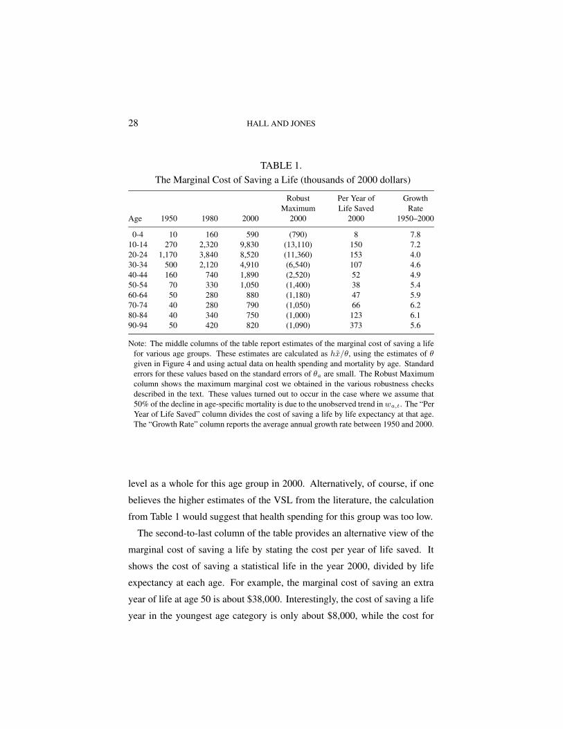
28 HALL AND JONES

TABLE 1.The Marginal Cost of Saving a Life (thousands of 2000 dollars)

Robust Per Year of GrowthMaximum Life Saved Rate

Age 1950 1980 2000 2000 2000 1950–2000

0-4 10 160 590 (790) 8 7.810-14 270 2,320 9,830 (13,110) 150 7.220-24 1,170 3,840 8,520 (11,360) 153 4.030-34 500 2,120 4,910 (6,540) 107 4.640-44 160 740 1,890 (2,520) 52 4.950-54 70 330 1,050 (1,400) 38 5.460-64 50 280 880 (1,180) 47 5.970-74 40 280 790 (1,050) 66 6.280-84 40 340 750 (1,000) 123 6.190-94 50 420 820 (1,090) 373 5.6

Note: The middle columns of the table report estimates of the marginal cost of saving a lifefor various age groups. These estimates are calculated as hx̃/θ, using the estimates of θgiven in Figure 4 and using actual data on health spending and mortality by age. Standarderrors for these values based on the standard errors of θa are small. The Robust Maximumcolumn shows the maximum marginal cost we obtained in the various robustness checksdescribed in the text. These values turned out to occur in the case where we assume that50% of the decline in age-specific mortality is due to the unobserved trend in wa,t. The “PerYear of Life Saved” column divides the cost of saving a life by life expectancy at that age.The “Growth Rate” column reports the average annual growth rate between 1950 and 2000.

level as a whole for this age group in 2000. Alternatively, of course, if one

believes the higher estimates of the VSL from the literature, the calculation

from Table 1 would suggest that health spending for this group was too low.

The second-to-last column of the table provides an alternative view of the

marginal cost of saving a life by stating the cost per year of life saved. It

shows the cost of saving a statistical life in the year 2000, divided by life

expectancy at each age. For example, the marginal cost of saving an extra

year of life at age 50 is about $38,000. Interestingly, the cost of saving a life

year in the youngest age category is only about $8,000, while the cost for


saving a life year for the oldest ages rises to well above $100,000. We discuss

the implications of this finding in a later section.

Finally, the last column of the table shows the growth rate for the marginal

cost of saving a life. Since the marginal cost is hx̃/θ and θ is constant over

time, these growth rates do not depend at all on the estimates of θ. The growth

rates are very high, on the order of 5 percent per year. By comparison, the em-

pirical VSL literature finds significantly lower growth rates. Taking income

growth to be about 2 percent per year, for example, the income elasticity from

Costa and Kahn (2003) of about 1.6 suggests that the VSL grows at a rate of

2 × 1.6 = 3.2 percent per year. This implies that the value of life in 1950 or

1960 would have been much higher than the marginal cost of saving a life.

Therefore, the U.S. may have been spending too little on health prior to the

most recent decade, even taking the level of the VSL from the lower end of

the estimates.

7. ESTIMATING THE PREFERENCE PARAMETERS

We present results for two approaches. The first treats the observed levels

of health spending as optimal and estimates the preference parameters. The

second estimates preference parameters from the evidence in the empirical

VSL literature; it implies that health spending was inefficiently low until the

end of the 20th century.

7.1. Treating Observed Health Spending as Optimal

Our model contains the following preference parameters: the discount fac-

tor β, the base levels of flow utility ba,t, the consumption parameter γ, the

quality-of-life parameter σ, and the weighting parameter α. For the moment,

we consider the case where health status does not affect flow utility so that

α = 0. We will reintroduce quality-of-life shortly.

30 HALL AND JONES

We have explored a variety of parametric restrictions on the base utility,

ba,t. These include making it a constant for all ages and years, making it

vary by age, and giving it a trend over time. The evidence in favor of age

effects is strong. There is evidence of trends in base utility, but not at the

same rate for different age groups. We have not found a useful parametric

restriction—candidates such as a set of age effects and a set of time effects re-

sult in sufficiently large residuals that the other parameters take on improbable

values.

Accordingly, we treat the values of ba,t as parameters themselves, without

imposing any restriction. Because there is one of these parameters for each

data point, estimation is a matter of solving for the values, not minimizing

a GMM norm or other criterion. Further, this means there are not enough

equations to estimate the other two parameters, β and γ. We use outside

evidence on these parameters before solving for the values of ba,t.

For the curvature parameter of the utility function, γ, we look to other

circumstances where curvature affects choice. Large literatures on intertem-

poral choice (Hall 1988), asset pricing (Lucas 1994), and labor supply (Chetty

2005) each suggest that γ = 2 is a reasonable value. Recall that higher values

of γ lead to faster growth in the value of life and therefore would deliver even

more rapid growth in the health share than what follows. With respect to the

discount factor, β, we choose a value that is consistent with this choice of γ

and with a 5 percent real return to saving. Taking consumption growth from

the data of 2.08 percent per year, a standard Euler equation gives an annual

discount factor of 0.992, or, for the 5-year intervals in our model, 0.963.

Given the data and the values of θa, β, and γ, we first calculate the implied

value of life from equation (21) and then recover the base levels of utility

from a rearranged version of equation (22). Figure 5 shows the results of the

calculations. Each line portrays the base level of utility for every age group in

a particular year, for the 11 years at 5-year intervals from 1950 though 2000.


FIGURE 5. Estimates of base flow utility, ba,t

0 20 40 60 80 100

−400

−200

0

200

400

600

Solved

Age

Note: Each line shows the cross section of base levels of utility in a given year. The periodscover 5 years each from 1950 through 2000. The heavy dashed line labeled “Solved” reportsthe set of base values inferred from the value of life in 2000 according to the model.

The lines share a common pattern—negative flow utility in the youngest group

and usually in the second-youngest group, and also negative flow utility for

teenagers. Negativity of flow utility does not contradict any principles of the

model. The motivation for continuing to live is to capture next period’s value

of life. Negative flow utility marks a difficult period of life that people choose

to live through so that they can enjoy later periods with positive utility. For

older people, flow utility stabilizes at a common, lower positive level over all

periods. Flow utility rises somewhat for the very elderly.

Alternatively, we can interpret the solved values for ba,t as the residuals from

the first-order condition in a model with a constant b. Economically, they arise

because the marginal cost of saving a life—the right side of equation (21),

32 HALL AND JONES

with values shown in Table 1—varies considerably more across ages than

the value of life on the preference side would in the absence of variation in

b. That is, with a constant b across ages, the value of life on the preference

side—the left side of equation (21)—turns out to be relatively flat across ages.

For example, consider the marginal cost of saving a life reported in Table 1.

The way the model interprets the fact that we spend so little on health care

for children from 0 to 4 and so much on those between 5 and 9, relative to

the marginal mortality reductions from spending, is by having a substantially

lower b for the younger group.

In the alternative interpretation of the estimates of ba,t as residuals, they

could be seen as measures, at different times, of the misallocation of health

care. The institutions that govern the delivery of health care may systemat-

ically fail to take advantage of opportunities to reduce infant mortality, for

example. This interpretation helps explain our finding that the ba,t do vary

over time, contrary to the hypothesis that they are unchanging parameters of

preferences.

These calculations provide estimates of the base level of utility during the

historical period. For our projections for the next 50 years, we need future

values of the base utility parameters. For this purpose, we make use of

additional information, namely the level of the value of life in utility units

from equation (21) in the last historical year, 2000. This level information

is not used in the calculation of the historical values of ba,t from equation

(22), which is in difference form. To make use of the level information, we

hypothesize that ba,t will not change over the future from its values in 2000.

This hypothesis makes sense, because there is no systematic trend in the

historical values in Figure 5. Then we proceed in the following way: When

we solve the model for the years 2000 through 2095, we treat ba as a set of

unknowns to solve and then require that the model solution match the value

of life in 2000. The heavy dashed line in Figure 5 shows these solved values.


Except for the more erratic values for the younger groups, the match is quite

good.

7.2. Matching the Earlier Value of Life Estimates

As an alternative approach to estimating the preference parameters, we

drop the assumption that the observed data are generated by maximizing

social welfare given our estimated health technology. Instead, we take the

age-specific spending data and the consumption data as given and compute

the value of life at each age, βva+1,t+1/uc, from these data. For future values

of health spending by age, we project the existing data forward at a constant

growth rate. Until the year 2020, this growth rate is the average across the

age-specific spending growth rates. After 2020 we assume spending grows

at the rate of income growth. The rate must slow at some point; otherwise

the health share rises above one. Our results are similar if we delay the date

of the slowdown to 2050.

We then estimate a constant and common value ba,t = b and the curvature

parameter γ to match some estimates from the VSL literature. Our baseline

scenario features a value of life for 35–39 year olds of $2 million in 1987.

We project this back to 1950 and forward to 2000, using a growth rate of

1.6 × 2.31 = 3.70 percent per year, based on the Costa and Kahn income

elasticity. By matching the value of life for this age group in 1950 and 2000,

we obtain b = 21.637 and γ = 1.624 for the case where health status does

not affect flow utility (i.e. α = 0). Finally, we recalibrate the time discount

factor β to an interest rate of 5 percent based on this new value of γ.

7.3. The Quality-of-Life Parameters

To calibrate the quality-of-life parameters σ and α, we draw upon the exten-

sive literature on quality-adjusted life years (QALYs), elicited by surveying

sick and healthy people, medical experts, and others—see Fryback et al.

34 HALL AND JONES

(1993) and Cutler and Richardson (1997). This work focuses on the QALY

weight, the flow utility level of a person with a particular disease as a fraction

of the flow utility level of a similar person in perfect health. Surveys ask

people what probability p of perfect health with probability 1 − p of certain

death would make them indifferent to their current health or what fraction of

a year of future perfect health would make them indifferent to a year in their

current health status. Both of these measures correspond to the relative flow

utility in our framework.

Cutler and Richardson (1997) estimate QALY weights by age. With new-

borns normalized to have a weight of unity, they find QALY weights of 0.94,

0.73, and 0.62 for people of ages 20, 65, and 85, in the year 1990. We use

these figures to estimate α and σ. For the case where ba,t is constant across

age and time, we use the two equations,

u(ct, x20,t)

.94=

u(ct, x65,t)

.73=

u(ct, x85,t)

.62,

for t = 1990 to solve for α and σ. Because the value of life itself depends on

these parameters, we estimate the utility parameters b and γ at the same time.

The resulting values are α = 1.922, σ = 1.051, b = 54.17, and γ = 1.593.

With four equations and four unknowns, estimation is a matter of solving for

the values, so there are no standard errors.

In addition to the QALY interpretation, these numbers can be judged in

another way. They imply that a 65 year-old would give up 88 percent of her

consumption, and an 85 year-old would give up 93 percent of her consumption

to have the health status of a 20 year-old. The intuition behind these large

numbers is the sharp diminishing returns to consumption measured by γ. To

explain what may seem to be a small difference in relative utilities of .94

versus .73 requires large differences in consumption. Health is extremely

valuable.


8. SOLVING THE MODEL

We now solve the model over the sample period 1950 through 2000 and

also project the economy out to the year 2050. We solve the model using

both of our approaches to calibrating the preferences parameters (the ba,t and

γ) and using two approaches to the quality of life (α = 0 and α > 0). For

the historical period, we take resources per person, y, at its actual value. For

the projections, we use the historical growth rate for the sample period, 2.31

percent per year. The details for the numerical solution of the model are

available from either author’s website.

Figure 6 shows the calculated share of health spending over the period

1950 through 2050. A rising health share is a robust feature of the optimal

allocation of resources in the health model. The key force at work in the

model behind this result is that the marginal utility of consumption in a given

period falls rapidly. As the U.S. gets richer and richer, the most valuable thing

people can purchase is more time to live.

The figure shows a substantial difference between projected health shares

for the two approaches. Our first approach matches the actual health share

between 1950 and 2000 exactly. The projection based on that approach im-

plies a rapidly growing health share in the future, reaching 33 percent in 2050.

The second approach, based on the VSL estimates in the literature, produces

a much flatter health share. Fundamentally, this slower rate of increase is

driven by the lower value of γ (1.6 versus 2.0) used in our second approach;

recall that γ governs the growth rate of the value of life and therefore de-

termines the growth rate of the health share. This second approach suggests

underspending on health for the last 50 years and generates a health share that

reaches 29 percent in 2050.

We conduct a number of robustness checks to illustrate how our benchmark

results change when key parameter values are varied in plausible ways. For

example, Figure 6 also shows what happens when health quality affects utility.

36 HALL AND JONES

FIGURE 6. Simulation Results: The Health Share of Spending

1950 2000 20500

0.05

0.1

0.15

0.2

0.25

0.3

0.35

0.4

Matching the value of life

(α=0)

(α>0)

Treating observed health spending as optimal

Actual

Year

Health Share, s

Circles “o” show actual data for the health share. The steeply-sloping line for the period2005-2050 show the projected health share assuming γ = 2, where the ba preferenceparameters are inferred from treating the historical data as if it were generated by the model.The gently sloping lines for the period 1950-2050 show the hypothetical historical andprojected share for preferences inferred from the VSL literature (e.g. γ = 1.62). Withinthese two approaches, the upper line corresponds to the case that includes a quality-of-lifeterm (α > 0), while the lower line does not (α = 0).

Our calibration of α and σ for this case implies a high willingness to pay for

health quality. As a result, overall health spending is higher in this scenario.

While our benchmark case leads to an optimal health share of just under 20

percent in 2000, allowing for quality of life in utility raises the share to 28

percent. The overall trend in the health share is quite similar.

Figure 7 shows several other robustness checks. Allowing for technical

change in the health sector to be one percentage point faster than in the

rest of the economy or reducing the share of mortality decline explained by

technical change and resource allocation from 2/3 to 1/2 deliver relatively


FIGURE 7. Robustness Checks: The Health Share of Spending

1950 2000 20500

0.05

0.1

0.15

0.2

0.25

0.3

0.35

0.4

Actual

Matching VSL: Faster Tech. Matching VSL:

50% health

Matching VSL: $3 million

Optimal:50% and Tech.

Year

Health Share, s

Circles “o” show actual data for the health share. This graph shows five alternativesimulations. For two of these alternatives, “Faster Tech.” and “50% health,” we considerboth the approach that treats observed spending as optimal and the approach that matchesa value of life in 1987 of $2 million. “Faster Tech.” assumes that technical change in thehealth sector is 1 percentage point faster than in the rest of the economy. “50% health”assumes that 1/2 of the decline in age-specific mortality (rather than our baseline valueof 2/3) is due to technological change and increased resource allocation. Finally, the fifthcase matches a value of life in 1987 for the 35–39 year olds of $3 million.

similar results. In both of these cases, less of the decline in age-specific

mortality is due to health spending, so the estimates of θa in the production

function are smaller. Since health spending runs into sharper diminishing

returns, the overall health share of spending is lower. These simulations

suggest that the observed share in the year 2000 was roughly optimal.

Alternatively, another robustness check in the figure assumes the value of a

stastical life is $3 million dollars in 1987 rather than $2 million. This means

the marginal benefit of health spending is higher, so the simulation delivers

38 HALL AND JONES

FIGURE 8. Health Spending by Age

0 20 40 60 80 100

400

1000

3000

8000

20000

60000

1950

2000

2050

Age

Constant 2000 dollars

Note: Circles denote actual data and solid lines show simulation results for the baselinesscenario in which b and γ are chosen to match estimates from the VSL literature.

a substantially higher health share. In 2000, for example, the optimal health

share is 26 percent, and it rises to 36 percent by 2050.

Figure 8 examines the micro data underlying the health share. This figure

shows actual and simulated health spending by age, for 1950, 2000, and 2050

for our second approach in the baseline scenario (in the first approach, actual

and simulated spending are equated by construction). A comparison of the

results for the year 2000 shows that actual and optimal spending are fairly

similar for most ages, with two exceptions. Optimal health spending on the

youngest age group is substantially higher than actual spending: given the

high mortality rate in this group, the marginal benefit of health spending is

very high, as was shown earlier. Similarly, while optimal health spending

generally rises until age 80, it declines after that point. It is worth noting in


FIGURE 9. Simulation Results: Life Expectancy at Birth

1950 2000 205068

70

72

74

76

78

80

82

Matching the value of life

Treating observed health spending as optimal

Actual

Year

Life Expectancy

See notes to Figures 6 and 7. Life expectancy is calculated using the cross-section distri-bution of mortality rates at each point in time.

this respect that the underlying micro data we use for health spending groups

all ages above 75 together, so we do not know what the actual pattern of

spending looks like above the age of 75.

Figure 9 shows the actual and projected levels of life expectancy at birth

for all eight of our simulation runs. The first thing to note in the figure

is the overall similarity of the life expectancy numbers. Because there are

such sharp diminishing returns to health spending in our health production

function, relatively large differences in health spending lead to relatively small

differences in life expectancy. A second thing to note is that the projected

path does not grow quite as fast as historical life expectancy. The reason is

again related to the relatively sharp diminishing returns to health spending

that we estimate.

40 HALL AND JONES

9. CONCLUDING REMARKS

A model based on standard economic assumptions yields a strong predic-

tion for the health share. Provided the marginal utility of consumption falls

sufficiently rapidly—as it does for an intertemporal elasticity of substitution

well under one—the optimal health share rises over time. The rising health

share occurs as consumption continues to rise, but consumption grows more

slowly than income. The intuition for this result is that in any given period,

people become saturated in non-health consumption, driving its marginal util-

ity to low levels. As people get richer, the most valuable channel for spending

is to purchase additional years of life.

This fundamental mechanism in the model is supported empirically in a

number of different ways. First, as discussed earlier, it is consistent with

conventional estimates of the intertemporal elasticity of substitution. Second,

the mechanism predicts that the value of a statistical life should rise faster

than income over time; Costa and Kahn (2003) and Hammitt et al. (2000) find

this to be the case. Cross-country evidence also suggests that health spending

rises more than one-for-one with income; this evidence is summarized by

Gerdtham and Jonsson (2000).

One source of evidence that runs counter to our prediction is the micro

evidence on health spending and income. At the individual level within the

United States, for example, income elasticities appear to be substantially less

than one, as discussed by Newhouse (1992). A serious problem with this

existing evidence, however, is that health insurance limits the choices facing

individuals, potentially explaining the absence of income effects. Our model

makes a strong prediction that if one looks hard enough and carefully enough,

one ought to be able to see income effects in the micro data. Future empirical

work will be needed to judge this prediction. A suggestive informal piece

of evidence is that exercise seems to be a luxury good: among people with


sedentary jobs, high wage people seem to spend more time exercising than

low wage people, despite the higher opportunity cost of their time.

As mentioned in the introduction, the recent health literature has empha-

sized the importance of technological change as an explanation for the rising

health share. In our view, this is a proximate rather than a fundamental ex-

planation. The development of new and expensive medical technologies is

surely part of the process of rising health spending, as the literature suggests;

Jones (2003) provides a model along these lines with exogenous technical

change. However, a more fundamental analysis looks at the reasons that new

technologies are developed. Distortions associated with health insurance in

the United States are probably part of the answer, as suggested by Weisbrod

(1991). But the fact that the health share is rising in virtually every advanced

country in the world—despite wide variation in systems for allocating health

care—suggests that deeper forces are at work. A fully-worked out techno-

logical story will need an analysis on the preference side to explain why it

is useful to invent and use new and expensive medical technologies. The

most obvious explanation is the model we propose in this paper: new and

expensive technologies are valued because of the rising value of life.

Viewed from every angle, our results support the proposition that both

historical and future increases in the health spending share are desirable.

The magnitude of the future increase depends on parameters whose values

are known with relatively low precision, including the value of life, how

rapidly that value has grown over time, and the fraction of the decline in age-

specific mortality that is due to technical change and the increased allocation

of resources to health care. Nevertheless, we believe it likely that maximizing

social welfare in the United States will require the development of institutions

that are consistent with spending 30 percent or more of GDP on health by the

middle of the century.

42 HALL AND JONES

REFERENCESAldy, Joseph E. and W. Kip Viscusi, “Age Variations in Workers’ Value of Statistical

Life,” December 2003. NBER Working Paper 10199.

Arthur, W. B., “The Economics of Risk to Life,” American Economic Review, March1981, 71 (1), 54–64.

Ashenfelter, Orley and Michael Greenstone, “Using Mandated Speed Limits to Mea-sure the Value of a Statistical Life,” Journal of Political Economy, February 2004,112 (1), S226–S267. Part 2.

Becker, Gary S., Tomas J. Philipson, and Rodrigo R. Soares, “The Quantity andQuality of Life and the Evolution of World Inequality,” American EconomicReview, March 2005, 95 (1), 277–291.

Card, David, Carlos Dobkin, and Nicole Maestas, “The Impact of Nearly Univer-sal Insurance coverage on Health Care Utilization and Health: Evidence fromMedicare,” 2004. NBER Working Paper No. 10365.

Chay, Kenneth Y. and Michael Greenstone, “The Impact of Air Pollution on InfantMortality: Evidence from Geographic Variation in Pollution Shocks Induced by aRecession,” Quarterly Journal of Economics, August 2003, 118 (3), 1121–1167.

Chetty, Raj, “Labor Supply and Risk Aversion: A Calibration Theorem,” 2005. U.C.Berkeley mimeo.

Costa, Dora and Matthew Kahn, “Changes in the Value of Life, 1940–1980,” May2003. MIT mimeo.

Cutler, David M. and Elizabeth Richardson, “Measuring the Health of the U.S. Popula-tion,” Brookings Papers on Economic Activity, 1997, Microeconomics, 217–282.

, Mark B. McClellan, Joseph P. Newhouse, and Dahlia Remler, “Are MedicalPrices Declining? Evidence from Heart Attack Treatments,” Quarterly Journalof Economics, November 1998, 113 (4), 991–1024.

Dow, William H., Tomas J. Philipson, and Xavier Sala-i-Martin, “Longevity Com-plementarities Under Competing Risks,” American Economic Review, December1999, 89 (5), 1358–1371.

Ehrlich, Isaac and Hiroyuki Chuma, “A Model of the Demand for Longevity and theValue of Life Extension,” Journal of Political Economy, August 1990, 98 (4),761–782.

and Yong Yin, “Explaining Diversities in Age-Specific Life Expectancies andValues of Life Saving: A Numerical Analysis,” September 2004. NBER WorkingPaper 10759.

Finkelstein, Amy and Robin McKnight, “What Did Medicare Do (And Was It WorthIt)?,” May 2005. NBER mimeo.


Fryback, Dennis G. et al., “The Beaver Dam Health Outcomes Study: Initial Catalogof Health-State Quality Factors,” Medical Decision Making, 1993, 13, 89–102.

Gerdtham, Ulf-G. and Bengt Jonsson, “International Comparisons of Health Ex-penditure: Theory, Data and Econometric Analysis,” in Anthony J. Culyer andJoseph P. Newhouse, eds., Handbook of Health Economics, North Holland, 2000.

Goldman, L. and E.F. Cook, “The decline in ischemic heart disease mortality rates:An analysis of the comparative effects of medical interventions and changes inlifestyle,” Annals of Internal Medicine, December 1984, 101 (6), 825–836.

Grossman, Michael, “On the Concept of Health Capital and the Demand for Health,”Journal of Political Economy, March/April 1972, 80 (2), 223–255.

, “Education and Nonmarket Outcomes,” in Eric Hanushek and Finis Welch, eds.,Handbook on the Economics of Education, Amsterdam: North-Holland, 2005.forthcoming.

Hall, Robert E., “Intertemporal Substitution in Consumption,” Journal of PoliticalEconomy, April 1988, 96 (2), 339–357.

Hammitt, James K., Jin-Tan Liu, and Jin-Long Liu, “Survival is a Luxury Good: TheIncreasing Value of a Statistical Life,” July 2000. Harvard University mimeo.

Heidenreich, Paul A. and Mark McClellan, “Trends in Treatment and Outcomesfor Acute Myocardial Infarction: 1975-1995,” American Journal of Medicine,February 15 2001, 110 (3), 165–174.

Jones, Charles I., “Why Have Health Expenditures as a Share of GDP Risen SoMuch?,” July 2003. U.C. Berkeley mimeo.

Kaplow, Louis, “The Value of a Statistical Life and the Coefficient of Relative RiskAversion,” July 2003. NBER Working Paper 9852.

Lucas, Deborah, “Asset Pricing with Undiversifiable Risk and Short Sales Constraints:Deepening the Equity Premium Puzzle,” Journal of Monetary Economics, 1994,34 (3), 325–342.

McClellan, Mark, Barbara J. McNeil, and Joseph P. Newhouse, “Does more intensivetreatment of acute myocardial infarction in the elderly reduce mortality? Analy-sis using instrumental variables,” Journal of the American Medical Association,September 1994, 272 (11), 859–866.

Meara, Ellen, Chapin White, and David M. Cutler, “Trends in Medical Spending byAge, 1963–2000,” Health Affairs, July/August 2004, 23 (4), 176–183.

Murphy, Kevin M. and Robert Topel, “The Economic Value of Medical Research.” InMeasuring the Gains from Medical Research: An Economic Approach (Murphyand Topel, eds 2003).

44 HALL AND JONES

and , eds, Measuring the Gains from Medical Research: An Economic Ap-proach, Chicago: University of Chicago Press, 2003.

Newhouse, Joseph P., “Medical Care Costs: How Much Welfare Loss?,” Journal ofEconomic Perspectives, Summer 1992, 6 (3), 3–21.

, Free for All? Lessons from the RAND Health Insurance Experiment, Cambridge,M.A.: Harvard University Press, 1993.

and Lindy J. Friedlander, “The Relationship between Medical Resources andMeasures of Health: Some Additional Evidence,” Journal of Human Resources,Spring 1980, 15 (2), 200–218.

Nordhaus, William D., “The Health of Nations: The Contribution of Improved Healthto Living Standards.” In Murphy and Topel, eds (2003).

Rosen, Sherwin, “The Value of Changes in Life Expectancy,” Journal of Risk andUncertainty, 1988, 1, 285–304.

Schelling, Thomas C., “The Life You Save May Be Your Own,” in Jr. Samuel B. Chase,ed., Problems in Public Expenditure Analysis, Washington D.C.: Brookings In-stitution, 1968, pp. 127–161.

Shepard, Donald S. and Richard J. Zeckhauser, “Survival versus Consumption,”Management Science, 1984, 30, 423–439.

Skinner, Jonathan, Elliott Fisher, and John E. Wennberg, “The Efficiency of Medi-care,” July 2001. NBER Working Paper 8395.

Usher, Daniel, “An Imputation to the Measure of Economic Growth for Changes inLife Expectancy,” in M. Moss, ed., The Measurement of Economic and SocialPerformance, New York: National Bureau of Economic Research, 1973.

Viscusi, W. Kip and Joseph E. Aldy, “The Value of a Statistical Life: A Critical Reviewof Market Estimates throughout the World,” Journal of Risk and Uncertainty,2003, 27, 5–76.

Weisbrod, Burton A., “The Health Care Quadrilemma: An Essay on TechnologicalChange, Insurance, Quality of Care, and Cost Containment,” Journal of EconomicLiterature, June 1991, 29, 523–552.

Wennberg, John E., Elliott S. Fisher, and Jonathan S. Skinner, “Geography and theDebate over Medicare Reform,” Health Affairs, February 13 2002, pp. W96–W114.

the value of life and the rise in health spending

Documents