the value of certainty in intellectual property rights

The Value of Certainty in Intellectual Property Rights:

Stock Market Reactions to Patent Litigation

Alan C. Marco

Department of Economics

Vassar College

Poughkeepsie, NY 12604-0708

845-437-7669

[email protected]

November 15, 2005

Vassar College Economics Working Paper # 82

Abstract

Using a sample of patents litigated between 1977 and 1997, I estimate stock market reactions to

patent litigation decisions and to patent grants. I find that the resolution of uncertainty over validity

and infringement is worth as much to the firm as the initial patent right. Each is worth about 1 to

1.5% excess returns. Additionally, I find that there are significant differences pre and post-1982 with

the establishment of the Court of Appeals for the Federal Circuit. I also find that there are significant

differences in reactions for plaintiff patent-holders and defendant patent-holders. Interestingly, there

is no similar effect for appellate court decisions relative to the district court. To my knowledge, this

is the first study that measures the stock market reactions to legal outcomes of patent cases.

Keywords: patents, uncertainty, litigation, innovation, event study

JEL codes: L19, L29, O32, O34, K41

1 Introduction

Legal uncertainty is inevitable in a patent rights system. And since patents are fundamentally prop-

erty rights, the legal environment can potentially significantly affect the value of patent protection

(Lanjouw 1994, Lemley and Shapiro 2005). Uncertainty over whether a “title” to property can be

enforced will undermine its market value: the title is only as good as the ability to enforce it.1 Legal

uncertainty is especially pervasive in emerging technology areas (or emerging patenting areas, like

business methods and software patents). Where uncertainty is prevalent, the effects on appropriation

and firm behavior can be dramatic.2 Since the purpose of a patent system is to provide incentives

for research, innovation, and diffusion by creating rewards, an inability to appropriate those rewards

diminishes the very incentives for which the system was designed.

Intellectual property managers face decisions about whether to patent innovations (Lerner 1995,

Grindley and Teece 1997, Hall and Ziedonis 2001), and how to manage market transactions in

intellectual property. Different legal or institutional environments may affect the incentives for firms

to license and do R&D (Reinganum 1989), to enter (Choi 1998), and to litigate (Meurer 1989). If

property rights are well-defined, firms may organize transactions through arms length negotiations.

In uncertain legal environments, we expect to see more integrated transactions ranging from cross-

1 Illustrative examples of the importance of property rights enforcement can be found in television portrayals of

the “Old West.” In 1859, a title to land in Virginia was more valuable than one in Nevada, in part because of the

“underlying value of the land,”–closer to transportation and markets, more fertile, etc. However, Virginia land was

also more valuable because better enforcement mechanisms were in place there. On the TV series Bonanza, the value

of the Ponderosa ranch was due in part to the quality of the land for grazing cattle, and in part to the ability of

the Cartwrights to enforce their title–whether through formal institutions (the local constabulary) or self-help (the

number of able-bodied Cartwrights available during the episode). See Ellickson (1991) for an excellent discussion of

formal versus informal dispute resolution.2The value of property rights is also affected by other institutional and technological factors, including standard-

setting and the availability of alternative mechanisms such as lead time, marketing, and trade secret. Uncertainty in

any of these areas will have impacts on appropriability.

1

licensing to strategic alliances to consolidation. To the extent that uncertainty affects or drives these

decisions, it is of great strategic importance to firms. And, to the extent that policy makers have some

control over the amount of legal uncertainty, or legal “quality” as coined by Merges (1999), it is an

important and understudied policy instrument. Simulation estimates (Lanjouw 1994, Lanjouw 1998)

find that changes in patent law or the legal environment can significantly change the value of patent

protection, not just for litigated patents, but for all patents even if none are ever litigated.3

Uncertainty is introduced into a patent system by both the administrative agency (the Patent

and Trademark Office (PTO) in the US) and the legal institutions. Because of the importance of

enforcement on the value of intellectual property, many researchers in the US have pointed to the

establishment of the Court of Appeals for the Federal Circuit (CAFC) in 1982 as a watershed in the

rights of patent holders. The CAFC established–among other things–a single court that would

hear the appeals of patent cases from all federal district courts (state courts do not hear patent cases).

It is claimed that the CAFC strengthened the rights of patent holders–that the court is more “pro-

patent” than its district peers (Lerner 1994, Lanjouw 1994, Lanjouw and Shankerman 1997, Kortum

and Lerner 1999, Henry and Turner 2006 (forthcoming)), so that we can expect a shift in the legal

standard in the early 1980s, perhaps increasing beliefs that a patent will be held valid and infringed.

The changes in the institutions governing patents can increase or decrease the uncertainty over

the scope and validity of patents, and we must recognize that this uncertainty will have effects on

firms’ incentives to litigate, license, do R&D, and to patent in certain areas. Lerner (1994) finds that

the “shadow” of litigation may change the patenting behavior of firms; in particular, high-litigation-

cost firms may target “less crowded” technology areas in order to avoid disputes. These effects may

be large, and may be an important part of the patent system. For this reason, it is important to

have an understanding of the quantitative impact of uncertainty on the value of patent rights.

The current political attention on tort reform in the US is evidence that policy-makers recognize

3For example, Lanjouw estimates that if the underlying probability of success for a plaintiff fell from 75% to 50%,and legal fees doubled, then the average patent value would be halved in her simulation, even if no cases were litigated.

2

the policy dimension of legal uncertainty on a broad scale. Since it is expensive for the administrative

agency to authenticate every patent, it may want to depend on individual firms to enforce their own

patents: it need not investigate each patent in depth. It may be more cost effective to introduce

some degree of uncertainty into the system as to the validity and scope of patents. In this way,

expenditure on each granted patent will be reduced, and only those which are in dispute will be

investigated (in court) at further cost. One can therefore expect the socially optimal amount of

uncertainty to be positive.

This paper presents an empirical investigation into the degree of uncertainty in granted US

patents. I make use of stock market reactions to court decisions and to patent grants in order

to estimate the magnitude of changes in beliefs about patent validity. It is from litigating that

market participants “learn” about the validity of patents from the court, and update their beliefs

accordingly. To my knowledge, this is the only study that measures stock market reactions to legal

outcomes of patent cases.

In this paper, I use an event study analysis for several reasons. First, litigation events are well

identified and there is little (if any) leakage about what the actual decision will be. Second, litigation

events can be directly associated with changes over a patent’s uncertainty. If a patent is ruled to

be valid, nothing about this decision affects the value of the underlying technology, so the change in

value reflects changes in beliefs about the uncertainty over property rights.

The primary result is that I find that market response to patent litigation tends to on par with

the market response to the patent grant itself. That is, the resolution of uncertainty about validity

or infringement is worth as much as the initial patent right on average, indicating the presence of

significant legal uncertainty. Secondly, I find there to be significant differences in market reactions

based on when the patent was adjudicated (before or after the establishment of the Court of Appeals

for the Federal Circuit in 1982) and whether the patent was owned by the plaintiff or defendant in

the suit. The intuition for the first result comes from option pricing theory. The fundamental value

3

of a patent right is the right to exclude others from using the technology. Since enforcement is

imperfect and costly (Lemley and Shapiro 2005), the right to exclude becomes the right to sue with

some probability of success (Marco 2005 forthcoming). Thus, in the property rights context, the

patent is an option to bring a lawsuit against an alleged infringer. Just like financial options, the

option to sue need not be exercised in order for it to have value, and the exercise of an option can

very well be worth more than the initial option value. Interestingly, I find no significant difference

between appeals and district court decisions.

Section 2 lays out the econometric specification, and Section 3 describes the patent data, litigation

data, and the event study results. In Section 4 I estimate several models that explain the size of

the market reactions, and that compare the effects of infringement suits (where the patent holder

brings the suit) to defensive suits (where the patent holder is the defendent). Section 5 concludes.

2 Empirical Model

Patent litigation is an especially useful area of law in which to examine market responses. First, the

question of validity is primarily a binary decision.4 The issue of infringement is not as straightfor-

ward, but the court’s decision still generally fits into a binary classification. Second, there is little

or no leakage prior to the announcement of the decision. Third, all the new information about the

patent pertains to changes in beliefs about the property right as opposed to the patented technology.

For patent i born at time 0, I assume that the value at time t can be approximated by

vit = pVit · pIit · zit

where V is the value of the patent, pV is the probability of winning on validity, pI is the probability

of winning on infringement, and z is some underlying private value of the technology were it to be

perfectly enforceable.4There are a handful of decisions where a patent is found valid in part and not valid in part. Those cases are

excluded from my sample.

4

If the patent is litigated at time τ , the change in patent value is given by

∆viτ = ∆pViτ · pIiτ · ziτ +∆pIiτ · pViτ · ziτ +∆pViτ ·∆pIiτ · ziτ (1)

where ∆ represents the change in the variable as a result of the court’s decision. Note that it

may be that ∆pViτ = 0 or ∆pIiτ = 0 if there is no decision on validity or infringement, respectively.

Importantly, I assume that the actual technological value, z, does not change as the result of the

court’s decision. Put another way, the court makes decisions only about the property right, and not

about the technology.

The econometric specification becomes

∆viτ = β0 +XViτβ1 +XI

iτβ2 +XV Iiτ β3 + εiτ (2)

where XViτ is a vector of variables that affect the market response to validity or invalidity decisions,

XIiτ is a vector of variables that affect the market response to infringement or non-infringement

decisions, and XV Iiτ is a vector of interaction terms between XV

iτ and XIiτ . In a simple specification,

I define XViτ =

£DViτ DNV

iτ

¤and XI

iτ =£DIiτ DNI

iτ

¤where the Ds are indicator variables for different

kinds of decisions: valid, not valid, infringed, not infringed. Note that I keep all the indicator

variables in the equation because DViτ +DNV

iτ may be equal to zero if there is no decision on validity

at date τ ; similarly with infringement. XV Iiτ then becomes

XV Iiτ =

£DViτ ·DI

iτ , DViτ ·DNI

iτ , DNViτ ·DI

iτ , DNViτ ·DNI

iτ

¤.

Note that the third term in equation 1, ∆pViτ ·∆pIiτ · ziτ , has only a second order effect. If thiseffect is negligible, the estimation equation becomes

∆viτ = β0 +XViτβ1 +XI

iτβ2 +XV Iiτ β3 + εiτ . (3)

It is clear from equation 1 that the change in the value of the patent will be a function of both

the marginal change in the expected probability of winning on validity and infringement and the

5

private value of the underlying technology. In a companion paper, I estimate a structural model

that attempts to disentangle these effects. For the current paper, I aim only to characterize the

distributions of stock market reactions to litigation decisions and to patent grants in order to infer

something about the value of resolution of legal uncertainty relative to the initial property right.

2.1 Multiple Patents-in-Suit

Before discussing the data and the calculation of excess returns and the probability of validity, one

econometric problem must be dealt with. I am not able to observe changes in patent value, but

rather changes in the value of a firm. So, if there are multiple “patents-in-suit” I observe only the

aggregate market reaction. Table 2 shows that of 295 adjudications, 209 involved a single patent.

the remaining 76 adjudications account for decisions on 266 patents. If there are N patents-in-suit

that are adjudicated simultaneously,

∆fiτ = ∆viτ1 +∆viτ2 + ...+∆viτN (4)

where ∆viτn represents the change in the value of patent n of firm i at time τ . So, while we observe

∆fiτ , what we seek is the expectation of ∆viτn given ∆fiτ , or E(∆viτn|∆fiτ ). In cases where N = 1

there is no difficulty in the estimation. Removing cases where N > 1 leaves information from

multiple patents-in-suit unexploited (and possibly biases the results). Instead, I use an application

of the Expectation-Maximization (EM) Algorithm to make use of the data when there are “missing”

∆viτn’s.5 The EMAlgorithm in this application is described in detail in Appendix A. The intuition is

that I estimate Equation (2) to predict values of ∆viτn for multiple patents-in-suit. These predicted

values are used in a new iteration of the estimation, and the process is repeated until the parameter

estimates converge.

5For a good overview of the EM Algorithm with applications to economics, see Ruud (1991); McLachlan and

Krishnan (1997) provide an extensive treatment of the subject.

6

3 Data

My data begin with a database compiled by researchers at the National Bureau of Economic Research

(NBER) and Case Western Reserve University (CWRU) (Hall, Jaffe and Trajtenberg 2000).6 The

sample consists of over 417,000 patents owned by publicly traded US manufacturing firms. The

patents are assigned Cusip identifiers using the 1989 ownership structure of the patent holder.

Litigation data were hand-collected from the United States Patents Quarterly (USPQ) 1977-

1997.7 The USPQ publishes annual indices containing patents on which adjudications were made

in that year. USPQ contains only “published” adjudications, which is a subset of all adjudications.

However, the advantage of the USPQ is that it contains clear information on the disposition of the

case with regard to validity and infringement. The USPQ data were merged with the NBER/CWRU

data to obtain a list of litigated patents owned by publicly traded firms.

The merged data contain 701 case citations involving 670 patents. I entered the disposition

data for each adjudication containing decisions relevant to validity or infringement.8 Adjudications

involving preliminary motions about discovery, jurisdiction, etc. were discarded. Also, PTO in-

terference proceedings and examination proceedings were not used. When a USPQ citation made

explicit reference to an earlier related decision, I incorporated that case into the database.

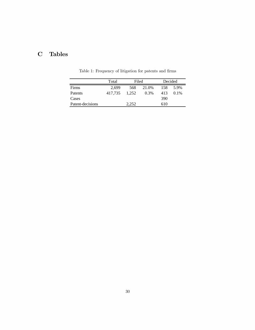
The final adjudication data consist of 390 decisions involving 413 patents owned by 158 publicly

traded firms. An observation in my data is a “patent-decision.” For example, a single case may

involve four patents. When a decision is made, I record four patent-decisions. In total, I have 610

patent-decisions. About half of the cases involve only one patent-decision. The implied litigation

rates are given in table 1, where case filing data was calculated using data obtained from LitAlert.9

In order to be able to analyze the adjudications using my methodology, I obtained CRSP data

6My thanks to Bronwyn Hall for permitting access to the data.7 See Allison and Lemley (1998) and Henry and Turner (2006 (forthcoming)).8The opinions themselves were obtained electronically from Lexis, to whom I am grateful for access to the USPQ

file.9 It is likely that both filing data and adjudication data are under-reported.

7

on daily stock returns from the Wharton Research Data Service (WRDS). Of the 390 adjudications,

ownership and returns data were available for 295. These 295 adjudications represent 325 patents

and 475 patent-decisions. Of those 325 patents, returns data were available for 287 patent application

dates and 309 issuance dates; for 283 patents, I have returns data for both dates.

Table 2 shows the break down of the 475 decisions into various subsamples. The first important

subsample is whether the case was decided in a lower court or a an appellate court. In my sample,

277 individual decisions were at the district court level. Note that my sample is subject to both

right-hand and left-hand truncation. That is, for a 1977 appellate decision, I would not have in my

sample the original lower court decision; for a 1997 lower court decision, I would not have in my

sample the subsequent appeal. In any case, one might expect appellate decisions to be weighted

differently by the market than district court decisions.

The next subsample shows that 125 cases occurred prior to 1982, when the Court of Appeals for

the Federal Circuit (CAFC) was established. This distinction is important for two reasons. First,

the CAFC is a centralized appellate court for patent cases. So, all appeals heard after that time

were heard in the same court. Second, the centralization may have led to a harmonization among

circuits in terms of precedent. Either of these may cause stock market reactions to differ pre- and

post-CAFC.

In most cases, the plaintiff is the patent holder. Only 48 decisions involve a defendant patent

holder. Market reactions between these two subsamples are likely to differ because of different

selection effects. Plaintiff patent holders engage in the typical patent infringement case. A patent

holder becomes a defendant in one of two instances: either it has been preemptively sued for a

declaratory judgment that the patent is invalid, or it has been sued for patent infringement, and it

counter-sues for infringement. In either case, defendent patent holders may have different incentives

to settle than plaintiff patent holders (Priest and Klein 1984, Waldfogel 1995). These different

selection effects may lead to different market responses.

8

As stated above, 209 observations obtain from single-patent adjudications, whereas 266 arise

from multiple-patent adjudications. Again, this problem leads to the use of the EM Algorithm to

disentangle the effects of contrasting decisions on the same date.

The last two rows of table 2 shows the breakdown by type of adjudication. 326 out of 475

patent decisions involved validity, and 298 involved infringement. Two important things should

be noted here. First, not every adjudication involves both infringement and validity. In many

trials, the issue of validity is determined separately from that of infringement. Frequently the trial is

bifurcated (or trifurcated): validity is determined first, and then infringement (and finally damages).

Settlement may occur at any phase of the trial. In my sample that case would show up as first a

validity adjudication, and some time later another adjudication on infringement. One trial, two

adjudications, unless settlement occurs. Further, in some trials, validity may not be questioned as

a defense. So, the court rules only on infringement. Thus, in my regression analysis, I code four

dummy variables to represent a ruling of validity (V ), invalidity (NV ), infringement (I), and non-

infringement (NI).10 Since any given adjudication can rule a patent valid, invalid, or can refrain

from ruling on validity (and similarly for infringement), I include all four dummy variables and a

constant in the estimation equation.

Another important piece of information is the relative frequency of validity rulings (326) relative

to infringement rulings (298). While the vast majority of suits are brought by the patent holder,

there are more validity rulings than infringement rulings. Clearly the validity of a patent is a

common defense. And, a patent holder should expect to face a decision on validity when it brings an

infringement suit. Among validity rulings, the win rate for the patent holder is 59%; for infringement

it is 64%. Additionally, the correlation coefficient between positive validity rulings and positive

10Technically, since validity is presumed, the court will rule that the patent is either invalid or not invalid. I refer

to valid and invalid patents for the sake of parsimony.

9

infringement rulings is 0.63. Defining the following variables as good news:

gV = V −NV

gI = I −NI,

I find that the correlation between gV and gI is 0.50.11

3.1 Event studies

As an estimate of the value to a patent holder of news about a patent, I rely on the event study

methodology. In particular I investigate two pieces of news: (1) news about the patent grant (at

the time of application and the time of issuance); and, (2) news about a court’s decision about the

validity or infringement of a patent. Event studies measure the change in the value of the firm using

cumulative abnormal returns, or excess returns. The methodology is the accepted way to tie stock

market valuations to particular events, but there are two caveats that should be mentioned.

First, if information about the event leaks into the market prior to the event date, then the

excess returns will measure only a portion of the total reaction. This problem is likely to be more

important for patent grants than for patent adjudications. The announcement effect of a patent

application or patent grant cannot be readily interpreted as representing the full value of the patent

because announcement effects only reflect changes in value with respect to news about the patent.

It is more likely that news about noteworthy patents may be known ahead of time. However, news

about a court’s decision is likely to be unknown prior to the decision.

Second, excess returns are notoriously noisy, since multiple factors can influence a stock price

on any given day. So long as those other factors are not systematically correlated with news about

patents, then they will add noise but will not bias the results.

11The correlation coefficients are based on individual patent decisions. Thus, they do not account for earlier decisions

by the same court on that patent.

10

Previous work on patent litigation and value has not explicitly made use of the information con-

tained in market responses to patent litigation decisions, or on the outcomes of court decisions. Some

renewal models use the incidence of litigation as well as renewal rates to estimate the parameters

of the model (Lanjouw 1998). But these papers do not look at legal outcomes. Allison and Lemley

(1998) investigate patent cases published in the US Patents Quarterly.12 The authors do investigate

the dispositions of these cases, but their focus is on the legal character of the cases more than the

economic implications.13

I use cumulative abnormal returns as measured by event studies to measure the stock market

reactions to patent decisions. Event studies are appropriate for several reasons. First, changes in

value are precisely what event studies are designed to measure. Second, while event studies have

been used by researchers to investigate the effects of other types of litigation (Bhagat, Brickley and

Coles 1994), no study has concentrated on patent litigation.14 Market reactions provide information

that has not been previously incorporated into the analysis of patent value. Third, litigation events

are well identified: court records for published decisions identify the date of the decision. Last,

litigation events can be directly associated with changes over beliefs about the legal patent right. If

a patent is ruled to be valid, nothing about the decision affects the value of the underlying technology,

so the change in value reflects changes in beliefs about the uncertainty over property rights.

In order to estimate equation 2, I need to calculate a measure for the market reaction to the

litigation event. The market model is the model most frequently used in event studies (Campbell,

Lo and MacKinlay 1997). The estimation equation is

Rit = αi + βiRmt + εit

12 I am grateful to Mark Lemley for alerting me to this source.13For instance, the incidence of certain legal defenses to infringement.14Austin (1993) uses event studies to examine market reactions to patent issuance.

11

where

Rit = proportionate return on the stock of firm i from time t− 1 to time t.

Rmt = proportionate return on the overall market from time t− 1 to time t.

Abnormal returns are calculated by estimating the parameters of the market model in some pre-

event equilibrium. Essentially, the abnormal return is the forecast error. The cumulative abnormal

returns are given by

CARit =

τ2Xt=−τ1

uit

That is, cumulative abnormal returns are the summation of abnormal returns over the event window

−τ1 to τ2, where the event occurs on day 0. For the analysis below the pre-event equilibrium is [-300,-20], measured in trading days. For the adjudication events, the abnormal returns are calculated

for symmetric event windows of 1, 3, 5, 7, 9, and 11 trading days around the event date, and an

asymmetric window of two days (day 0 and day +1). For patent grants, I drop the one day window.

The Equal Weighted Market Return is used for Rm, as defined by CRSP.

4 Analysis

4.1 Excess returns

Tables 3 and 4 summarize the results of the event studies. The first column lists the event window

used to calculate the excess returns, 2 to 11. Additionally, I calculate a bootstrap sample. For a

single bootstrap replication, a sample of patents (with replacement) is drawn from my sample. For

each patent a single event window is randomly chosen. The distribution given in the table represents

the distribution of 500 bootstrap replications. The random event window is admittedly arbitrary.

However, it is less arbitrary than choosing a single event window for all application and issuance

12

dates.15

It is evident from table 3 that the application date produces a significant positive reaction from

the market, in constrast to both the issuance date and the sum of the returns at the application and

issuance dates. This may seem strange in light of US patent laws: applications are not made public,

whereas patents themselves are. However leakage is important in this context, because important

patents may have more information leaked near the application date than near the issuance date.

Austin (1993) performs event studies on a sample of biotechnology patents and determines that the

patent grant date is more appropriate.

For all windows greater than two days, the 90% confidence interval shows positive excess returns

around the patent application date. For nine- and 11-day windows, the sum of the application

and issuance date returns is also significantly positive. The 11-day returns show a response of

1.4% to 2% for the application date, and 1.2% to 3.3% for the sum of application and issuance

returns. The bootstrap estimates show a smaller confidence interval of 0.14% to 1.0% at the date

of application. Finally, bootstrap estimates show a dollar value (calculated from excess returns and

market capitalization) of $28.1 million at the mean, and a 90% confidence interval of $0.7 million to

$55.4 million.

To put this in context, compare these reactions to the excess returns estimates of patent issuance

done by Austin (1993). He finds that excess returns range from a mean of about $500,000 for the full

sample, to a mean of $33 million for those patents mentioned in the Wall Street Journal. If litigated

patents comprise a sample of the most valuable patents (Allison, Lemley, Moore and Trunkey 2003),

the comparison to “Wall Street Journal” patents is apt.

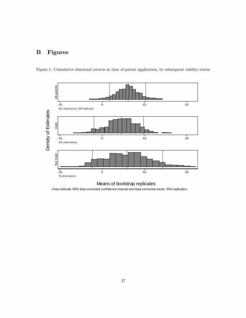
Table 4 and figures 1 and 2 present excess returns at application date by the patent’s later

15 It is unlikely that a single event window would represent all firms equally well. In the absence of a prior as to

which window would work better for different types of firms or patents, I rely on the more robust bootstrapping

estimator of the mean.

13

infringement or validity status,16 as determined by the court. Do patents that are later found to be

valid or infringed show higher excess returns at the time of birth? The short answer is no. In fact,

the histograms in figures 1 and 2 show that excess returns at the date of application are likely to be

slightly higher for invalidated or not infringed patents than for valid or infringed patents, although

the difference is not statistically significant. Patents that are later found valid have mean excess

returns of 0.46% compared to 0.59% for patents that are later found invalid. Similarly, infringed

patents have mean excess returns at the date of application of 0.53% compared to 0.99% for non-

infringed patents. Only the non-infringed result is significantly different from zero at the 10% level.

The lower returns for subsequently valid and infringed patents is not completely surprising and is

almost certainly due to a selection effect. There may be some uncertainty over the strength of the

original property right for patents that are later litigated. If a patent holder has private information

about a patent’s validity (Meurer 1989), it will be more likely to pursue litigation if the market’s

perception of the patent is particularly low relative to the patent holder. Thus, the low returns to

later validated patents may be a signal of the market’s perception of value, rather than the patent

holders.

Table 4 and figure 3 present the excess returns by type of disposition at the time of adjudication.

The results of the response at adjudication is meaningless in the aggregate because they contain

information for both good news and bad news events, as well as “mixed” events (e.g., a valid but

not infringed patent). We expect the market returns to be somewhat noisy despite the precision of

the event date. First, firms differ in size, so reactions to good or bad news about patents will vary

not only according to revision in beliefs, but also according to the firm’s market capitalization. Large

firms will have smaller responses, ceteris paribus. Additionally, there will be individual heterogeneity

at the patent level because of the heterogeneity in the underlying technological value. I control for

this heterogeneity by using the log of the dollar returns as the dependent variable, and by using a

random effects model.16For the current tables and figures, and those that follow, the bootstrap estimates of the distribution are presented.

14

It is evident that the mean reaction to infringement is positive and the mean reaction to non-

infringement is negative. Validity leads to a positive response, but invalidity leads to an even higher

positive response. In fact, of the four types of dispositions, only invalidity is significantly different

from zero (at the 10% level). The market reactions to adjudications are confounded by two factors.

First, multiple-patent decisions mistate the market reaction to any individual patent that is a part

of the decision. If two patents are adjudicated simultaneously, and the decision is that one patent is

valid and infringed, and one patent is not valid, then the market reaction will be a combination of

the response to each patent.17 Secondly, the decision on an individual patent may be a mix of good

news and bad news, e.g., valid and not infringed or invalid and infringed.18

Because of the confounding influences affecting market reactions to adjudication, it is appropriate

to turn to regression analysis to disentangle the effects of multiple patens and mixed decisions.

4.2 Regression results

Table 5 presents the results of estimating a variation of equation 3

CARit = β0 + Vitβ1 +NVitβ2 + Iitβ3 +NIitβ + εit. (5)

where CAR indicates the cumulative abnormal return at the time of adjudication from the event

studies. All estimations use the EM Algorithm described in appendix A, and all standard errors

are bootstrapped (1000 replications). Since the bias in the estimates relative to the bootstrap

replications tended to be large (usually greater than 0.25 of the standard error), bias corrected

17Cases in the sample contain as many as 12 patents.18Oddly enough, the latter decision is not unheard of. Six observations in my data are valid and not infringed.

District courts began the practice in recognition that their decision on validity might be overturned on appeal. This

is the consequence of anticipated appeals on the part of district courts. If an invalidity decision is overturned by the

Court of Appeals for the Federal Circuit, then it can expedite proceedings to decide both issues at the time of the

original trial, rather than have a separate trial on remand. In that instance, the court would save time to rule on

both matters simultaneously. See, for example, Datascope Corp. v. SMEC, Inc. (224 USPQ 694 [1984]) N.J.

15

coefficients are reported and significance levels are determined from the bias-corrected confidence

intervals rather than from the bootstrapped standard errors (Efron and Tibshirani 1993, Briggs,

Wonderling and Mooney 1997).

The first model uses the two-day excess returns as the independent variable. The second model

uses another application of the bootstrap, similar to that used in examining the means of the

excess returns in section 4.1. Each replication consists of a sample of 475 observations drawn from

the sample (with replacement). The event window is then chosen randomly for each observation

from the set {1, 2, 3, 5, 7, 9, 11} as above. The rationale is the same as with the means: there is nojustification for choosing any particular event window since the appropriate window is likely to differ

on the basis of the individual patent, company, and decision. Thus, I choose a random window for

each observation. The bootstrapping procedure yields consistent estimates.

The third model in table 5 estimates a random effects version of equation 5

CARit = β0 + Vitβ1 +NVitβ2 + Iitβ3 +NIitβ + ui + εit, (6)

where ui is a patent specific disturbance term and εit is the standard disturbance term. In addition

to the ordinary parameter estimates, the random effects model estimates parameters σu and ρ, the

proportion of the overall variance associated with σu as opposed to σε. Lastly, the fourth model

estimates a random effects model with the log of the dollar value of the excess returns as the

dependent variable. The remaining regressions all use the bootstrapped random effects model with

the EM Algorithm.

Model 1 (using the two-day window) shows a significant value for NV (not valid) decisions

only. The estimated market reaction is −1.25%. Model 2 yields no significant results. However therandom effects model estimates the parameters with much more precision. Again, from equation

1, the market response will depend on the value of z (the underlying technological value). The

heterogeneity embedded in z is approximated by the random effects model.

The coefficients show a 1.6% excess return due to validity, −1.4% return from invalidity, a

16

−1.8% response to a non-infringement ruling, and a 0.8% response in the constant term; reaction

to infringement is not measured precisely. Note that the constant term reflects a positive market

reaction to the conclusion of a case. This is not unexpected since the resolution of uncertainty

tends to be favored by the market. Additionally, providing certainty about validity, invalidity or

infringement is worth about 1.5% to the firm. That is, more certain property rights are worth as

much to the firm as the estimates of patent value at the time the patent is born (around 1%).

The estimate of ρ is quite high, indicating that much of the unobserved heterogeneity is patent

specific (as opposed to observation specific), which is consistent with the idea that the random

effects model captures the heterogeneity embedded in zi. The log dollars equation confirms only the

negative coefficient on invalidity. It is interesting that the dollars equation does not more accurately

measure the coefficients, since some of the noise in excess returns arises from differences in firm size.

However, it is standard in the event study literature to use excess returns rather than dollar values,

and in this instance it does not appear to harm the precision of the estimates (as long as the random

effects model is used).

Table 6 compares the simple random effects model (model 3 of table 5) to an estimation that

includes the interaction terms according to equation 2. The interaction terms are mostly insignificant,

and most of the coefficients on the primary disposition variables also become insignificant (including

the constant term). The exceptions are the validity coefficient of 3.4% (significant at the 99% level)

and the valid and not infringed interaction term of −4.9% (significant at the 95% level). These

coefficients are much larger than without the interaction terms. Several of the other coefficients

are large in magnitude but imprecisely measured, probably due to the presence of multicolinearity

among the regressors. For the remaining regressions, I rely on the non-interacted model for the

sake of simplifying the interpretation. That restriction does affect the results on the subsample

regressions below.

In table 2, I described several different subsamples that might affect the size of market reactions

17

to patent adjudications and the resolution of uncertainty in patents. The next section investigates

those subsamples in more detail.

4.3 Subsamples

Table 2 listed three ways to divide the sample:

1. appeals versus district court decisions,

2. pre- and post-1982 decisions, and

3. plaintiff patent holders and defendant patent holders.

For each pair of complementary subsamples, I use a Chow test to determine whether the coeffi-

cients of each subsample are different from one another (using the random effects model on excess

returns in table 5). Based on non-bias-corrected coefficients, none of the subsamples have a signifi-

cant effect; the largest Chi-squared statistic (five degrees of freedom) is 8.1, with a p-value of only

0.15.

Two of the three Chow tests using the bias-corrected coefficients were significant. Comparing the

pre- and post-1982 decisions led to a statistic of 16.7 (p-value < 0.01). Reactions to plaintiff patent

holders were significantly different from defendant patent holders, with a statistic of 13.0 (p-value <

0.05). It is very interesting that the appellate decisions did not lead to larger market responses than

lower court decisions, on average (chi-squared statistic of 3.2, p-value = 0.67). One would think that

the higher courts would have final say on validity and infringement (since very few patent cases go

to the Supreme Court), and that markets would respect this greater power. While this may be true,

the effect is not large enough to show in the data. However, the pre- and post-CAFC era does seem

to make a difference, whether at the appellate level or the district level.

Tables 7 and 8 compare the results of estimating equation 5 for the pre- and post-CAFC era, and

for plaintiff and defendant patent holders, respectively. Interestingly, the post-CAFC era is charac-

18

terized by smaller excess returns in response to validity and larger (negative) responses to invalidity.

Pre-CAFC reactions to infringement decisions were much larger than post-CAFC responses (and

both infringement and non-infringement led to negative responses). Taken together, a valid and

infringed patent had a neglible market reaction prior to the establishment of CAFC, and the loss on

infringement was a significant negative. This indicates that only very strong patents (patents that

were believed to be likely to win) were being litigated because the response to the upside was small,

and the response to the downside was large.

There is an intriguing results with regard to plaintiff and defendant patent-holders. Market re-

actions tend to be larger with validity decisions for plaintiffs and for infringement decisions with

defendants. On the surface this may seem strange, since plaintiff cases are usually straight infringe-

ment cases, and defendant cases usually deal with validity (decaratory judgments for invalidity).

However, this result has to do with selection, expectations, and uncertainty. Since plaintiff cases

are brought with regard to infringement, it may be that the markets well predict the infringement

outcome relative to the validity outcome. Similarly, since defendant cases are usually brought with

respect to validity, the markets may well predict the validity outcome in comparison to the infringe-

ment outcome. Additionally, the constant term is significant (1.8%) for defendant cases. Because

defendant cases are–in a sense–involuntary on the part of the defendant, there existence signals

greater risk to the company than a lawsuit deemed necessary for the protection of the firm’s property.

Thus, the conclusion of such a case is likely to be more valuable to defendant patent-holders.

Separating the subsamples leads to one surprising result: that appellate courts do not generate

more significant market responses than lower courts. Additionally, the comparision of pre- and post-

1982 and plaintiff and defendant patent-holders highlights the impacts of selection on the returns to

litigation.

19

5 Conclusion

By investigating the size of the market reactions–and how they differ systematically among cases–I

am able to make some inferences about the value of certainty in patent rights. This paper is the first

to estimate market reactions to patent litigation events, and to compare them to market reactions

at patent birth. The primary result is that the resolution of uncertainty is as valuable to the firm as

the initial patent grant (which is subject to uncertainty). If the sample is at all representative, then

this result is an indication that there may be a significant amount of legal uncertainty created by

the patent system. For some models, merely the conclusion of a case is worth a 1% return, similar

in magnitude to the original patent grant.

Additionally, I find that firms can expect validity rulings whether the patent is owned by the

plaintiff or defendant. This result is important because patent validity is one source of asymmetry

of stakes, which is very important in the selection literature (Priest and Klein 1984, Waldfogel 1995,

Marco 2004). If a patent-holder expects to face a decision on validity, then the opportunity cost

of an invalid patent (that affects negotiations with all potential licensees) becomes a significant

litigation cost (near −1.5% return in my estimates). On the other hand, a win on validity has a

similarly asymmetric upside. However, since returns to validity decisions are similar to returns on

infringement decisions, it may be that a ruling on infringement can lead to similar asymmetry.

One very important caveat should be mentioned about the results. They are conditional on

litigation. This is, of course, obvious because the sample consists entirely of litigated patents.

However, because selection effects are well-known this sample does not represent in any way a

random sample of patents.

On the other hand, to the extent that litigated patents represent a sample of valuable patents

(Allison et al. 2003), then the results are important. If valuable patents are subject to uncertainty

about validity and infringement, then resolving that uncertainty is important to patent holders.

Leaving the uncertainty unresolved reduces patent value and the rewards to innovation (Lemley

20

and Shapiro 2005). Perhaps this is warranted: it may be that the patenting authorities wish to

accomodate some uncertainty in the system (Cockburn, Kortum, and Stern, 2002). However, to the

extent that uncertainty in the patent system is unintentional, then the reduction in patent value is

certain to be suboptimal.

Legal uncertainty in patent policy may actually be an unexploited policy tool (Marco 2005

forthcoming). Uncertainty is likely to be high in emerging technology (or emerging patenting areas,

such as business method patents). This may be exactly those areas where policy makers wish

uncertainty to be high (or rather, for rewards to be low). As cases are litigated, and precedent

becomes clearer, the uncertainty is reduced and rewards are increased (or decreased) appropriately.

Treating uncertainty as a policy tool is predicated on the recognition that the current patent system

creates uncertainty. This paper takes a step towards measuring the degree to which that uncertainty

is economically meaningful.

21

References

Allison, John R. and Mark A. Lemley, “Empirical evidence on the validity of litigated patents,”

AIPLA Quarterly Journal, Summer 1998, 26 (3).

, , Kimberley A. Moore, and R. Derek Trunkey, “Valuable Patents,” Public Law

and Legal Theory Research Paper No. 133 (U.C. Berkeley School of Law), 2003.

Austin, David H., “An event-study approach to measuring innovative output: The case of biotech-

nology,” AEA Papers and Proceedings, May 1993, 83 (2), 253—258.

Bhagat, Sanjai, James A. Brickley, and Jeffrey L. Coles, “The costs of inefficient bargaining

and financial distress,” Journal of Financial Economics, 1994, 35, 221—247.

Briggs, Andrew H., David E. Wonderling, and Christopher Z. Mooney, “Pulling Cost-

Effectiveness Analysis Up by Its Bootstraps: A Non-Parametric Approach to Confidence Inter-

val Estimation,” Health Economics, 1997, 6, 327—340.

Campbell, John Y., Andrew W. Lo, and A. Craig MacKinlay, The Econometrics of Finan-

cial Markets, Princeton University Press, 1997.

Choi, Jay Pil, “Patent litigation as an informational-transmission mechanism,” American Eco-

nomic Review, December 1998, 88 (5), 1249—1263.

Efron, B. and R. Tibshirani, An Introduction to the Bootstrap, New York: Chapman and Hall,

1993.

Ellickson, Robert C., Order without law: How neighbors settle disputes, Cambridge: Harvard

University Press, 1991.

Grindley, Peter C. and David J. Teece, “Managing intellectual capital: Licensing and cross-

licensing in semiconductors and electronics,” California Management Review, Winter 1997, 39

(2), 1—34.

22

Hall, Bronwyn H., Adam Jaffe, andManuel Trajtenberg, “Market value and patent citations:

A first look,” NBER Working Paper 7741 June 2000.

and Rosemarie Ham Ziedonis, “The Patent Paradox Revisited: An Empirical Study

of Patenting in the U.S. Semiconductor Industry, 1979-1995,” RAND Journal of Economics,

Spring 2001, 32 (1), 101—128.

Henry, Matthew D. and John L. Turner, “The Court of Appeals for the Federal Circuit’s

Impact on Patent Litigation,” Journal of Legal Studies, January 2006 (forthcoming), 35.

Kortum, Samuel and Joshua Lerner, “What is Behind the Recent Surge in Patenting?,” Re-

search Policy, January 1999, 28 (1), 1—22.

Lanjouw, Jean O., “Economic consequences of a changing litigation environment: The case of

patents,” NBER Working Paper 4835 August 1994.

, “Patent protection in the shadow of infringement: Simulation estimations of patent value,”

Review of Economic Studies, 1998, 65, 671—710.

and Mark Shankerman, “Stylized facts of patent litigation: Value, scope and ownership,”

NBER Working Paper 6297 December 1997.

Lemley, Mark A. and Carl Shapiro, “Probabilistic Patents,” Journal of Economic Perspectives,

Spring 2005, 19 (2), 75—98.

Lerner, Joshua, “The importance of patent scope: An empirical analysis,” Rand Journal of Eco-

nomics, Summer 1994, 25 (2), 319—333.

, “Patenting in the shadow of competitors,” Journal of Law and Economics, October 1995,

pp. 463—495.

Marco, Alan C., “The Selection Effects (and Lack Thereof) in Patent Litigation: Evidence from

Trials,” Topics in Economics Analysis and Policy, 2004, 4 (1).

23

, “The Option Value of Patent Litigation: Theory and Evidence,” Review of Financial Eco-

nomics, 2005 forthcoming.

McLachlan, Geoffrey J. and Thriyambakam Krishnan, The EM algorithm and extensions,

John Wiley & Sons, 1997.

Merges, Robert P., “As many as six impossible patents before breakfast: Property rights for

business concepts and patent system reform,” Berkeley Technology Law Journal, 1999, 14, 577—

615.

Meurer, Michael J., “The settlement of patent litigation,” Rand Journal of Economics, Spring

1989, 20 (1), 77—91.

Priest, George L. and Benjamin Klein, “The selection of disputes for litigation,” Journal of

Legal Studies, January 1984, 13, 1—55.

Reinganum, Jennifer F., “The timing of innovation: Research, development, and diffusion,” in

R. Schmalansee and R. D. Willig, eds., Handbook of Industrial Organization, Volume I, Elsevier

Science Publishers B.V., 1989, chapter 14, pp. 850—908.

Ruud, Paul A., “Extensions of estimation methods using the EM algorithm,” Journal of Econo-

metrics, 1991, 49, 305—341.

Waldfogel, Joel, “The selection hypothesis and the relationship between trial and plaintiff victory,”

Journal of Political Economy, 1995, 103 (2), 229—260.

24

A EM Algorithm

The EM Algorithm enables me to estimate the change in the value of a particular patent given that

I know the change in the value of the firm, and the disposition of the patent in question and other

simultaneously adjudicated patents. That is, the EM Algorithm enables me to estimate values for

∆v conditional on ∆f for the special case where the ∆v’s are missing. Since multiple patents may

be adjudicated simultaneously, the excess returns for the firm’s stock price must be apportioned

across the ∆v’s. To do so, we require E(∆viτn|∆fiτ ,Xiτn) where Xiτn is a vector of characteristics

of the disposition of the case. Let

∆viτn = Xiτnβ + εiτn

where

εiτn ∼ N¡0,σ2

¢so that the error term is normal and the εiτn’s are independently and identically distributed. The

assumption of independence is convenient but not innocuous. We can imagine that patents that

are litigated together may not be independent, but instead be part of a larger system. The validity

of any component may rise and fall by the validity of the system. The potential dependence of

component patents warrants investigation; however, for simplicity I will assume independence in

this paper.

Since I assume that ∆fiτ =P

N ∆viτn, I can write

∆fiτ ∼ N

ÃXN

Xiτn,Nσ2

!

and

V ar(∆viτn) = σ2

V ar(∆fiτ ) = Nσ2

Cov(∆viτn,∆fiτ ) = σ2.

25

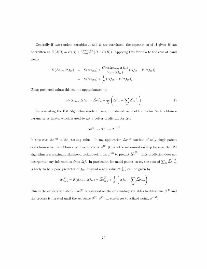
Generally if two random variables A and B are correlated, the expectation of A given B can

be written as E (A|B) = E (A) + Cov(A,B)V ar(B) (B −E (B)). Applying this formula to the case at hand

yields

E (∆viτn|∆fiτ ) = E(∆viτn) +Cov(∆viτn,∆fiτ )

V ar(∆fiτ )(∆fiτ −E(∆fiτ ))

= E(∆viτn) +1

N(∆fiτ −E(∆fiτ )) .

Using predicted values this can be approximated by

E (∆viτn|∆fiτ ) = d∆viτn + 1

N

Ã∆fiτ −

XN

d∆viτn! (7)

Implementing the EM Algorithm involves using a predicted value of the vector ∆v to obtain a

parameter estimate, which is used to get a better prediction for ∆v:

∆v(0) → β(0) → c∆v(1)In this case ∆v(0) is the starting value. In my application ∆v(0) consists of only single-patent

cases from which we obtain a parameter vector β(0) (this is the maximization step because the EM

algorithm is a maximum likelihood technique). I use β(0) to predict c∆v(1). This prediction does notincorporate any information from ∆f . In particular, for multi-patent cases, the sum of

PNc∆v(1)iτn

is likely to be a poor predictor of fiτ . Instead a new value ∆v(1)iτn can be given by

∆v(1)iτn = E(∆viτn|∆fiτ ) = c∆v(1)iτn +

1

N

Ã∆fiτ −

XN

c∆viτn!

(this is the expectation step). ∆v(1) is regressed on the explanatory variables to determine β(1) and

the process is iterated until the sequence β(0), β(1), ... converges to a fixed point, βEM .

26

B Figures

Figure 1: Cumulative abnormal returns at time of patent application, by subsequent validity status

All

pa

tent

s

- .01 0 .01 .02282 observat ions , 500 replicates

Va

lid

- .01 0 .01 .02105 observat ions .

Not

Va

lid

- .01 0 .01 .0276 observations.

Den

sity

of E

stim

ates

Means of bootstrap replicatesLines indicate 90% bias-corrected confidence interval and bias-corrected mean. 500 replicates.

27

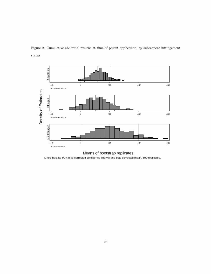
Figure 2: Cumulative abnormal returns at time of patent application, by subsequent infringement

status

All

pa

tent

s

- .01 0 .01 .02 .03282 observat ions .

Infr

ing

ed

- .01 0 .01 .02 .03109 observat ions .

Not

In

frin

ge

d

- .01 0 .01 .02 .0378 observations.

Den

sity

of E

stim

ates


28

Figure 3: Cumulative abnormal returns at time of adjudication, by dispositionV

alid

- .02 -.01 0 .01 .02 .03193 observat ions .

Not

Va

lid

- .02 -.01 0 .01 .02 .03133 observat ions .

Infr

ing

ed

- .02 -.01 0 .01 .02 .03190 observat ions .

Not

In

frin

ge

d

- .02 -.01 0 .01 .02 .03108 observat ions .

Den

sity

of E

stim

ates


29

C Tables

Table 1: Frequency of litigation for patents and firms

Total

Firms 2,699 568 21.0% 158 5.9%Patents 417,735 1,252 0.3% 413 0.1%Cases 390 Patent-decisions 2,252 610

Filed Decided

30

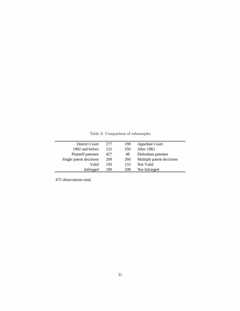
Table 2: Comparison of subsamples

District Court 277 198 Appellate Court1982 and before 125 350 After 1982

Plaintiff patentee 427 48 Defendant patenteeSingle patent decisions 209 266 Multiple patent decisions

Valid 193 133 Not ValidInfringed 190 108 Not Infringed

475 observations total.

31

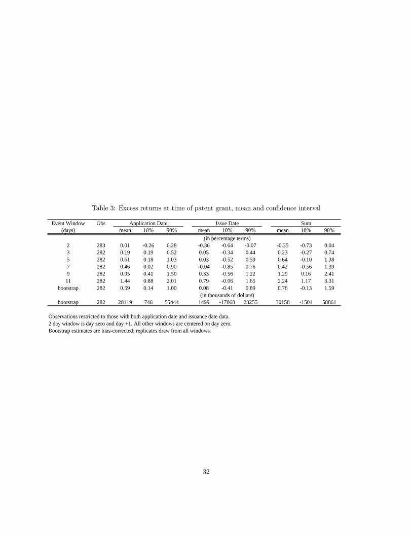
Table 3: Excess returns at time of patent grant, mean and confidence interval

Event Window Obs(days) mean 10% 90% mean 10% 90% mean 10% 90%

2 283 0.01 -0.26 0.28 -0.36 -0.64 -0.07 -0.35 -0.73 0.043 282 0.19 0.19 0.52 0.05 -0.34 0.44 0.23 -0.27 0.745 282 0.61 0.18 1.03 0.03 -0.52 0.59 0.64 -0.10 1.387 282 0.46 0.02 0.90 -0.04 -0.85 0.76 0.42 -0.56 1.399 282 0.95 0.41 1.50 0.33 -0.56 1.22 1.29 0.16 2.4111 282 1.44 0.88 2.01 0.79 -0.06 1.65 2.24 1.17 3.31

bootstrap 282 0.59 0.14 1.00 0.08 -0.41 0.89 0.76 -0.13 1.59

bootstrap 282 28119 746 55444 1499 -17068 23255 30158 -1501 58861

Observations restricted to those with both application date and issuance date data.2 day window is day zero and day +1. All other windows are centered on day zero.Bootstrap estimates are bias-corrected; replicates draw from all windows.

(in percentage terms)

(in thousands of dollars)

Application Date SumIssue Date

32

Table 4: Excess returns at time of patent grant, mean and confidence interval, by disposition

Sampleobs mean 10% 90% obs mean 10% 90%

All 282 0.62 0.19 1.08 -- -- -- --Valid 105 0.46 -0.17 1.06 193 0.44 -0.21 1.23

Not Valid 76 0.59 -0.10 1.56 133 0.95 0.11 1.98Infringed 109 0.53 0.11 0.91 190 0.28 -0.54 1.05

Not Infringed 78 0.99 -0.01 1.96 108 -0.28 -0.99 0.55

Bootstrap estimates are bias-corrected; replicates draw from all windows.

(in percentage terms)

Application Date Adjudication Date

33

Table 5: Effects of case disposition on firm value

Variable Coef. Coef. Coef. Coef.

Valid 0.63 -0.08 1.54 0.44 -0.40 1.33 1.59 ** 0.28 3.06 1.28 -0.91 3.77(0.49) (0.53) (0.80) (1.39)

Not Valid 0.59 * -1.25 -0.08 -0.52 -1.29 0.23 -1.43 ** -2.99 -0.40 -3.29 *** -5.72 -1.20(0.35) (0.46) (0.68) (1.28)

Infringed 0.53 -1.54 0.10 -0.31 -1.23 0.52 -0.78 -1.97 0.37 0.01 -2.24 2.47(0.50) (0.53) (0.73) (1.39)

Not Infringed 0.15 -0.76 0.40 0.09 -0.67 0.90 -1.79 *** -2.60 -0.78 -0.92 -3.34 1.30(0.36) (0.48) (0.62) (1.42)

Constant 0.27 -0.29 0.83 0.23 -0.45 0.90 0.83 * 0.01 1.83 0.80 -0.86 2.60(0.34) (0.42) (0.52) (1.05)

Sigma e -- -- 1.35 2.78Sigma u -- -- 2.83 4.75Rho -- -- 0.82 0.74Chi2 -- -- 280 133F 2.21 9.69 -- --R2 overall 0.010 0.010 0.012 0.019Observations 475 475 475 475Replications 1000 1000 1000 1000

Bootstrapped SE in paranthesis. Bias-corrected confidence intervals used to calculate significance level.* indicates p < 0.1, ** indicates p < 0.05, *** indicates p < 0.01.All coefficients and confidence intervals are bias-corrected.

[3]CAR

EM/RE/bootstrap

[4]ln(dollars)

EM/RE/bootstrap

[1]CAR2

EM

[2]CAR

EM/bootstrap90% conf. int. 90% conf. int. 90% conf. int. 90% conf. int.

34

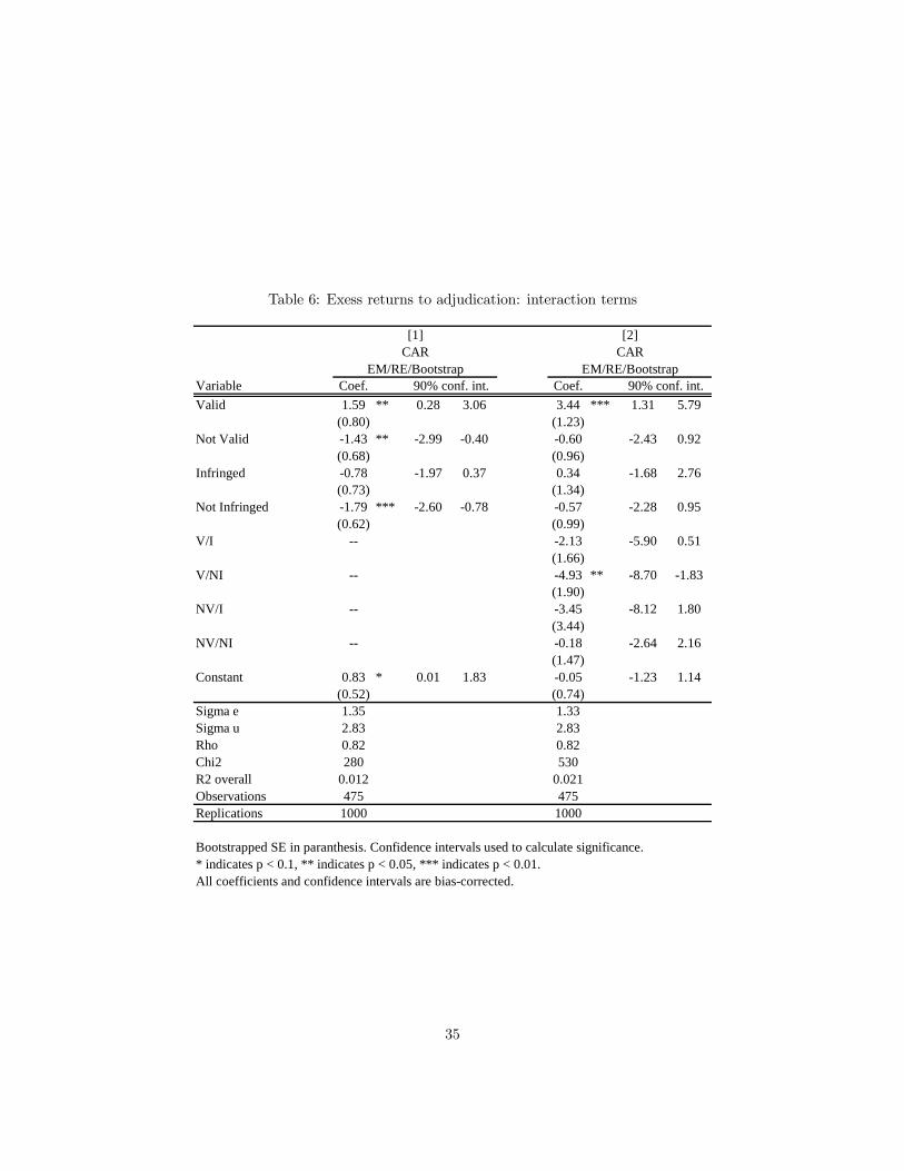
Table 6: Exess returns to adjudication: interaction terms

Variable Coef. Coef.

Valid 1.59 ** 0.28 3.06 3.44 *** 1.31 5.79(0.80) (1.23)

Not Valid -1.43 ** -2.99 -0.40 -0.60 -2.43 0.92(0.68) (0.96)

Infringed -0.78 -1.97 0.37 0.34 -1.68 2.76(0.73) (1.34)

Not Infringed -1.79 *** -2.60 -0.78 -0.57 -2.28 0.95(0.62) (0.99)

V/I -- -2.13 -5.90 0.51(1.66)

V/NI -- -4.93 ** -8.70 -1.83(1.90)

NV/I -- -3.45 -8.12 1.80(3.44)

NV/NI -- -0.18 -2.64 2.16(1.47)

Constant 0.83 * 0.01 1.83 -0.05 -1.23 1.14(0.52) (0.74)

Sigma e 1.35 1.33Sigma u 2.83 2.83Rho 0.82 0.82Chi2 280 530R2 overall 0.012 0.021Observations 475 475Replications 1000 1000

Bootstrapped SE in paranthesis. Confidence intervals used to calculate significance.* indicates p < 0.1, ** indicates p < 0.05, *** indicates p < 0.01.All coefficients and confidence intervals are bias-corrected.

[1] [2]CAR

EM/RE/Bootstrap90% conf. int. 90% conf. int.

EM/RE/BootstrapCAR

35

Table 7: Adjudications pre- and post-1982


Valid 3.31 * 0.01 6.51 2.21 *** 0.90 3.90(2.01) (0.85)

Not Valid -0.93 -4.22 2.45 -1.32 * -3.89 -0.12(2.01) (0.88)

Infringed -4.09 ** -6.95 -1.54 -0.60 -2.04 0.80(1.57) (0.88)

Not Infringed -5.40 *** -7.96 -3.40 -1.18 * -2.96 -0.02(1.27) (0.79)

Constant 1.50 -1.99 4.32 0.41 -0.52 1.55(1.88) (0.61)



90% conf. int. 90% conf. int.

[1] [2]Pre-1982 Post-1982

36

Table 8: Defendant and plaintiff patentees


Valid 1.67 ** 0.32 3.85 -0.34 -2.23 1.45(0.92) (1.14)

Not Valid -1.47 * -3.84 -0.16 -2.67 -5.37 0.12(0.81) (1.65)

Infringed -0.93 -2.72 0.47 1.22 * 0.15 2.31(0.94) (0.67)

Not Infringed -1.31 * -3.32 -0.15 -1.70 ** -3.81 -0.29(0.78) (1.02)

Constant 0.72 -0.37 2.29 1.77 ** 0.35 3.45(0.68) (0.94)



90% conf. int.

[1] [2]Plaintiff patentee Defendant patentee

90% conf. int.

37

the value of certainty in intellectual property rights

Documents