the validation and improvement of route-based road weather forecasts · 2012-12-14 · the...
TRANSCRIPT

THE VALIDATION AND IMPROVEMENT OF
ROUTE-BASED ROAD WEATHER FORECASTS
by
DAVID STUART HAMMOND
A thesis submitted to
The University of Birmingham
for the degree of
DOCTOR OF PHILOSOPHY
School of Geography, Earth & Environmental Sciences
The University of Birmingham
January 2011

University of Birmingham Research Archive
e-theses repository This unpublished thesis/dissertation is copyright of the author and/or third parties. The intellectual property rights of the author or third parties in respect of this work are as defined by The Copyright Designs and Patents Act 1988 or as modified by any successor legislation. Any use made of information contained in this thesis/dissertation must be in accordance with that legislation and must be properly acknowledged. Further distribution or reproduction in any format is prohibited without the permission of the copyright holder.

ABSTRACT
This thesis aims to develop the foundations for a new validation strategy for route-based road
weather forecasts that will enable validation of route-based models at a vastly improved
spatial and temporal resolution, and in doing so provide a tool for rapid appraisal of new
model parameterisations. A validation strategy that uses clustering techniques to create
clusters of forecast points with similar geographical and infrastructure characteristics is
presented, as well as two methodologies for de-parameterising key geographical and
infrastructure parameters in the ENTICE route-based model that are currently not measured at
the spatial scale demanded by a route-based forecast. The proposed validation strategy
facilitates the analysis of forecast statistics at the cluster level, which is shown to provide a
more representative measure of the model’s spatial forecasting ability. The majority of
thermal variations around the study route are well represented by the clustering solutions,
presenting the opportunity for new sampling strategies with the potential to validate forecasts
at a vastly improved spatial and temporal resolution. De-parameterisation of the road
construction and surface roughness parameters within the ENTICE model using Ground
Penetrating Radar and airborne LIDAR data has been shown to significantly improve the
spatial forecasting ability of ENTICE, with the model changes leading to refinement of the
clustering solution which enables it to better capture the physical relationship between road
surface temperature and the geographical and infrastructure parameters around the study
route. Suggestions for future research are provided along with a blueprint for the future of
route-based road weather forecasts.

ACKNOWLEDGMENTS
Firstly, I must acknowledge the financial support of Weather Services International and the
University of Birmingham for funding this project. This thesis is in many ways a continuation
of the work started by Dr Lee Chapman over a decade ago, whose supervision, advice and
friendship over the past 3 years has been greatly appreciated. A big thank you must also go to
Professor John E. Thornes for his supervision over the past 6 years including the KTP project
with Campbell Scientific. I’ve now been associated with the University of Birmingham for 7
years, firstly as an MSc student, then as a KTP research associate, and finally as a doctoral
researcher, and over this time I’ve made many new friends. A big thank you to all the friends
I’ve had the pleasure of knowing during my years at Birmingham.
A few people at Birmingham who deserve a special mention include Richard Johnson for his
expert workmanship in designing a mobile infrared sensor mount out of a bike rack, Jill
Crossman for assisting with GPR data collection (at very short notice!) and Kevin Burkhill for
his continual assistance with drawings. Thank you also to the editors and anonymous referees
involved in the peer review of papers submitted from this thesis, whose comments and
suggestions for improvement have helped to refine this final work.
During the writing of this thesis many hours were spent working at home, and special thanks
have to go to Max for the many afternoon walks which came as a welcome distraction.
Finally, thank you to my wife, Laura, whose constant support over the past 3 years has not
gone unnoticed.
10 January 2011

CONTENTS PAGE
CHAPTER 1: INTRODUCTION
1.1 Winter Road Maintenance…………………………………………………………………. 1
1.2 The History of Road Weather Information Systems………………………………………. 4
1.2.1 Road danger warnings……………………………………………………………….. 5
1.2.2 Ice detection…………………………………………………………………………. 6
1.2.3 Ice prediction……………………………………………………………………….. 11
1.2.4 Route-based forecasting……………………………………………………………. 20
1.3 Aims and Objectives……………………………………………………………………... 23
1.3.1 Aims………………………………………………………………………………... 23
1.3.2 Objectives…………………………………………………………………………... 23
Chapter One Summary……………………………………………………………………….. 25
CHAPTER 2: A NEW VALIDATION STRATEGY FOR ROUTE-BASED ROAD
WEATHER FORECASTS
2.1 Existing Validation Techniques………………………………………………………….. 26
2.1.1 Road outstations……………………………………………………………………. 26
2.1.2 Remote infrared temperature sensors………………………………………………. 27
2.1.3 Thermal mapping…………………………………………………………………... 30
2.2 Data Reduction…………………………………………………………………………… 34
2.2.1 Techniques for data reduction……………………………………………………… 35
2.2.2 Data reduction in the ENTICE route-based forecast model………………………... 38
2.2.2.1 Building the ENTICE GPD…………………………………………………. 38
2.2.2.2 Birmingham study route……………………………………………………..40
2.2.2.3 Modifications to the ENTICE GPD………………………………………….42
2.3 Hierarchical and K-means Clustering of the ENTICE GPD……………………………... 45
2.4 Consistency of the Clustering Techniques……………………………………………… 56
2.5 Comparison of Hierarchical and K-means Clustering…………………………………… 58
2.6 Implementing a Cluster Based Validation Strategy…………………………………….. 59
Chapter Two Summary……………………………………………………………………….. 61

CHAPTER 3: SPATIAL RE-PARAMETERISATION OF THE ENTICE MODEL:
PART 1 - ROAD CONSTRUCTION
3.1 Road Construction Modelling in Route-Based Forecasts………………………………... 62
3.2 Ground Penetrating Radar………………………………………………………………... 65
3.2.1 Calculating layer depth……………………………………………………………...66
3.2.2 GPR traces and radargrams………………………………………………………… 67
3.3 Application of GPR Data within the ENTICE Model……………………………………. 68
3.3.1 Data collection………………………………………………………………………68
3.3.2 Identification of bridge decks from radargrams……………………………………. 70
3.3.3 Subsurface layer depths…………………………………………………………......73
3.3.4 Surface heat flux…………………………………………………………………… 82
3.4 Statistical Analysis of New Subsurface Parameterisation…………………………...…... 84
Chapter Three Summary……………………………………………………………………... 90
CHAPTER 4: SPATIAL RE-PARAMETERISATION OF THE ENTICE MODEL:
PART 2 – SURFACE ROUGHNESS
4.1 Surface Roughness……………………………………………………………………….. 91
4.2 Existing Z0 Parameterisation in ENTICE………………………………………………… 93
4.3 New Methodology for Z0 Estimation in ENTICE………………………………………... 96
4.3.1 Roughness length estimation………………………………………………………..96
4.3.2 Height based rule of thumb………………………………………………………… 98
4.3.3 Local Z0 estimation from LIDAR data……………………………………………... 99
4.3.4 Calculating effective Z0……………………………………………………………100
4.4 Changes to ENTICE to Enable Inclusion of Z0eff
……………………………………….. 112
4.4.1 Z0eff
values………………………………………………………………………… 112
4.4.2 Wind direction…………………………………………………………………….. 112
4.5 Statistical Analysis of New Z0eff
Values……....…………………………………………114
Chapter Four Summary……………………………………………………………………...118
CHAPTER 5: SPATIAL VALIDATION OF THE ENTICE ROUTE-BASED
FORECAST MODEL
5.1 Summary of Overall Model Performance………………………………………………. 119
5.2 K-means Clustering of the New ENTICE GPD………………………………………… 123
5.3 Consistency of the New K-means Clustering Solution………………………………... 129
Chapter Five Summary………………………………………………………………………131

CHAPTER 6: CRITIQUE AND SUGGESTED IMPROVEMENTS
6.1 Critique of Techniques………………………………………………………………….. 132
6.1.1 GPR road construction data………………………………………………………..132
6.1.2 LIDAR based Z0eff
values…………………………………………………………. 134
6.2 Traffic Parameterisation………………………………………………………………… 136
6.2.1 Impacts of traffic on RST…………………………………………………………. 136
6.2.2 Existing traffic parameterisation in the ENTICE model…………………………...137
6.2.3 Potential alternative modelling techniques………………………………………...138
6.2.4 Pilot study – traffic counting with infrared RST sensor…………………………...141
6.2.5 Other potential sources of traffic density data……………………………………..146
6.3 A Blueprint for the Next Generation of Route-Based Forecasts………………………...151
Chapter Six Summary……………………………………………………………………….. 156
CHAPTER 7: CONCLUSIONS 157
REFERENCES 162
APPENDICES
1. MATLAB HIERARCHICAL CLUSTER PROGRAM
2. GPR TRACE INFLEXION POINT FLOW CHART
3. IRIS DATALOGGER PROGRAM
4. TRAFFIC DATA
5. MODIFIED ENTICE MODEL
6. PEER REVIEWED PUBLICATIONS

LIST OF FIGURES
1.1 Average annual weather related fatalities in the US, based on data from the
National Center for Atmospheric Research, Boulder, Colorado 1
1.2 Skid resistance as a function of temperature 2
1.3 Significant events in the history of UK road weather forecasting 5
1.4 Possible sources of error in the forecast and treatment of icy roads using road
danger warnings 6
1.5 A Vaisala Road Surface Analyser (ROSA) outstation monitoring road surface
and atmospheric conditions 7
1.6 Thermal fingerprints showing the variation in residual (average) road surface
temperature for the same route at different levels of atmospheric stability 9
1.7 Thermally mapped data plotted in a GIS environment (Leicestershire,
10/02/08) 10
1.8 Example RST forecast curve 14
1.9 Schematic of the National Ice Prediction Network 16
2.1 An IRIS remote infrared temperature sensor monitoring road surface
temperatures at the Eurotunnel freight terminal in Folkestone, UK.
Photograph courtesy of Campbell Scientific Ltd 28
2.2 Example Pareto chart for showing the variance explained by each principal
component 36
2.3 Map displaying the mixed urban and rural study route in Birmingham, UK,
which was used as the test bed for the research in this thesis 41
2.4 Geographical and infrastructure parameters from the ENTICE GPD plotted as
layers in a GIS, showing variations in geographical and infrastructure
parameters around the Birmingham study route for (a) altitude; (b) land use;
(c) road type; (d) ψs 42
2.5 Top section of a dendrogram showing the hierarchical clustering solution for
the Birmingham study route GPD generated using the Euclidean metric and
group average clustering algorithms. The horizontal line across the
dendrogram intersects 12 links on the cluster tree, demonstrating the
partitioning of the dataset into 12 clusters 48
2.6 (a) A map of the hierarchical clustering solution for the Birmingham study
route, together with a summary GPD showing the mean values within each
hierarchical cluster 51
(b) A map of the K-means clustering solution for the Birmingham study
route, together with a summary GPD showing the mean values within each
K-means cluster 52
3.1 The influence of road construction on RST modelling at different levels of
atmospheric stability, using actual RST data from 20 thermal mapping runs
for comparison of model performance. The standard deviation of each
thermal mapping run is used as a proxy to stability 63
3.2 A sample GPR trace, showing the varying amplitude of the electromagnetic
pulse as it penetrates the subsurface 67
3.3 (a) Radargram collected on a motorway showing a deep and uniform road
construction
(b) Radargram collected on a minor c-road showing a less uniform, shallower
construction 68
3.4 Equipment setup showing the Malå RoadCart in action 69
3.5 Location, radargrams and typical magnitude of the known thermal
singularities (under stable conditions) of four bridge decks on the study route 71
3.6 Aerial photograph of the motorway bridge identified in Figure 3.5 (c),
showing the location of traffic lights on the bridge which often leads to
standing traffic causing the warm thermal singularity of +0.3°C observed at
this location 72
3.7 Calculated depths of subsurface interfaces at each forecast point along the
study route, assuming a five zone flexible pavement with material
composition matching that of the existing ENTICE road construction
parameterisation shown in Table 3.1 75
3.8 Comparison of ENTICE model accuracy in predicting RST to within ± 1°C of
actual values. X-axis values relate to model runs using the original ENTICE
road construction parameterisation, and y-axis values relate to model runs
using the new variable subsurface measurements derived from GPR data 88
3.9 R2 values for ENTICE predicted RST vs. actual RST collected from thermal
mapping runs. X-axis values relate to model runs using the original ENTICE
road construction parameterisation, and y-axis values relate to model runs
using the new variable subsurface measurements derived from GPR data 88
3.10 Sample METRo model code displaying the existing road layer
parameterisation, into which the new subsurface layers depths derived from
GPR data could easily be added 90
4.1 Eight landuse classes around the study route as defined by the OWEN
landuse classification 103
4.2 Illustration of effective roughness length (Z0eff
) calculation for each 2 m
LIDAR grid cell over distances of upwind fetch ranging from 100 m up to
500 m, assuming a westerly prevailing wind 104
4.3 Variation in maximum Z0eff
values around the study route with approaching
wind direction 109
4.4 (a) Standard deviation of Z0eff
values at each forecast point around the study
route over the eight wind directions shown in Error! Reference source not
found.
(b) Enlarged view of a rural section of the study route, revealing a forested
area acting as a natural screen to approaching northerly to westerly winds 111
4.5 Excerpt from the ENTICE GPD database file, showing the new LIDAR based
Z0eff
values appended to the end of the database. 112
4.6 Excerpt from an ENTICE comma separated raw meteorological input data
file, showing the wind direction appended to the end of each row. 113
4.7 Comparison of ENTICE model accuracy in predicting RST to within ± 1°C of
actual values. X-axis values relate to model runs using the original ENTICE
ordinal based Z0 values, and y-axis values relate to model runs using the new
LIDAR based Z0eff
values 117
4.8 R2 values for ENTICE predicted road surface temperature vs. actual road
surface temperature collected from thermal mapping runs. X-axis values
relate to model runs using the original ENTICE ordinal based Z0 values, and
y-axis values relate to model runs using the new LIDAR based Z0eff
values 117
5.1 Average RMSE values for ENTICE predicted RST over the Birmingham
study route (20 nights). X-axis values relate to model runs before any changes
were made to the ENTICE model, and y-axis values relate to model runs

which incorporate the de-parameterised surface roughness and road
construction measurements 121
5.2 Comparison of ENTICE model accuracy in predicting RST to within ± 1°C of
actual values. X-axis values relate to model runs before any changes were
made to the ENTICE model, and y-axis values relate to model runs which
incorporate the de-parameterised surface roughness and road construction
measurements 122
5.3 R2 values for ENTICE predicted RST vs. actual RST collected from thermal
mapping runs. X-axis values relate to model runs before any changes were
made to the ENTICE model, and y-axis values relate to model runs which
incorporate the de-parameterised surface roughness and road construction
measurements 123
5.4 A map of the new K-means clustering solution for the Birmingham study
route, together with a summary GPD showing the mean values within each
cluster 125
6.1 (a) Differential drying on the E4 highway north of Gävle, Sweden
(approximately 60.5°N), showing how heat fluxes from traffic dry the road
surface on the heavily trafficked inside lane
(b) Thermal image of the southbound M5 carriageway where frictional heat
dissipation from tyre tracks is clearly evident 137
6.2 Hierarchical semantic clustering flowchart for the two spatial characteristics
of region and density 140
6.3 IRIS sensor monitoring traffic flow at the site of an active loop detector as
part of a pilot study into traffic parameterisation in route-based forecast
models 141
6.4 Hourly vehicle count data over 7 days (Mon 28/06/10 – Sun 04/07/10) from
an IRIS infrared RST sensor (blue line) compared against data collected from
a loop detector at the same location (red line) 142
6.5 System architecture for the ESA Road Traffic Monitoring by Satellite
(RTMS) trial 148
6.6 Sample METRo model code for imposing a minimum wind speed at
difference times of the day to account for increased turbulence caused by
vehicles 150
6.7 UK Met Office route-based forecasting graphical user interface 152
6.8 Schematic of the proposed next generation route-based forecasting system 154

LIST OF TABLES
2.1 Potential sources of error in thermal mapping 31
2.2 Meteorological, geographical and road infrastructure parameters used to drive
the ENTICE road weather prediction model 39
2.3 (a) Correlation matrix for the Birmingham GPD, showing the strength of
correlations between the various geographical and infrastructure parameters
(b) p-values matrix for the Birmingham GPD indicating the significance of
the correlations 44
2.4 (a) Route-based forecast validation statistics for the study route calculated for
individual hierarchical clusters
(b) The same as (a), but for K-means clustering 55
2.5 Minimum, maximum, mean and SD of RST (°C) and category of thermal
mapping (TM) fingerprint 57
2.6 Clustering similarity coefficients (CSC) for independent pairs of thermal
mapping runs in the same weather category, calculated using hierarchical
clustered forecast points (a) and K-means clustered forecast points (b) 58
2.7 SPSS output statistics for an Independent samples t test comparing clustered
GPD values for the hierarchical and K-means clustering solutions 59
3.1 The materials and thermal properties of the ordinal road construction profiles
used in ENTICE 62
3.2 Average depths for each layer of the de-parameterised five zone flexible
pavement in the ENTICE model, based on analysis of the digitised
electromagnetic waveform data from a GPR survey using an algorithm
(Appendix 2) designed to identify subsurface interfaces from significant
inflexions in the waveform of individual GPR traces 76
3.3 Forecast statistics from a statistical analysis on average thermal conductivity
profiles in ENTICE, where all geographical variables in the model were held
constant with the exception of road type 80
3.4 Forecast statistics from a statistical analysis on road construction
parameterisation in the ENTICE model. Statistics in Analysis 1 relate to
modelled vs. actual RST using the original ENTICE road construction
parameterisation, and statistics in Analysis 2 relate to modelled vs. actual
RST using the new de-parameterised subsurface road construction
measurements derived from GPR data 86
4.1 Updated Davenport classification of terrain roughness 92
4.2 Z0 values (cm) currently used in the ENTICE model in relation to the ordinal
landuse and road type classification 95
4.3 Minimum recommended upwind fetch distances (m) for various types of
surface cover. 101
4.4 Kruskal-Wallis results for Z0eff
comparisons between OWEN landuse classes 106
4.5 Wilcoxon P-values matrices comparing Z0eff
values between each OWEN
landuse class over five distances of upwind fetch 107
4.6 Forecast statistics from a statistical analysis on surface roughness in ENTICE,
where all geographical variables in the model were held constant with the
exception of surface roughness 115

5.1 ENTICE route-based forecast validation statistics for the Birmingham study
route calculated for individual K-means clusters 127
5.2 Clustering similarity coefficients (CSC) for independent pairs of thermal
mapping runs in the same weather category, calculated using the new K-
means clustered forecast points 130
6.1 Traffic similarity coefficients (TSC) for pairs of traffic count data in the same
6-hourly time period, calculated using traffic count data from a loop detector
and estimates of traffic count from an IRIS sensor postioned at the same
location as the loop detector 145

LIST OF ABBREVIATIONS AND SYMBOLS
AADT Annual Average Daily Traffic
ANOVA Analysis of Variance
BADC British Atmospheric Data Centre
CSC Clustering Similarity Coefficients
DEM Digital Elevation Model
DSM Digital Surface Model
DTM Digital Terrain Model
ESA European Space Agency
EWMA Exponentially Weighted Moving Average
FHWA Federal Highway Administration
FSL Forecast Systems Laboratory
GIS Geographical Information System
GPD Geographical Parameter Database
GPR Ground Penetrating Radar
GPRS General Packet Radio Service
GPS Global Positioning System
GSM Global System for Mobile Communications
IP Internet Protocol
LIDAR Light Detection and Ranging
MDSS Maintenance Decision Support System
METRo Model of the Environment and Temperature of the Roads
MIDAS Motorway Incident Detection and Automatic Signalling
MORST Met Office Road Surface Temperature Model
NWP Numerical Weather Prediction
PCA Principal Components Analysis
RCTM Road Condition and Treatment Module
RMSE Root Mean Square Error
RST Road Surface Temperature
RWFS Road Weather Forecast System
RWIS Road Weather Information System
SD Standard Deviation
TM Thermal Mapping
TSC Traffic Similarity Coefficients
UK United Kingdom

US United States
USB Universal Serial Bus
VDT Vehicle Data Translator
VFM View Factor Mapping
VII Vehicle Integrated Infrastructure
XML Extensible Markup Language
ϐ Bias
σϐ Standard deviation of bias
ε Surface emissivity
εsky Effective emissivity of the sky
ρ Air density
Γ Dry adiabatic lapse rate
α Albedo
a Adiabatic exchange coefficient
σ Stefan Boltzmann constant
ψs Sky view factor
c Speed of light in free space (m s-1
)
C Heat capacity of air
cal cm-1
sec-1
°C Calorie (IT) per centimetre per second per degree Celsius
d Thermal diffusivity
d’ Bulk adiabatic diffusivity
di Thickness of ith layer
εr,i Dielectric constant of ith layer
E Surface energy flux
H Sensible heat flux to air
Inet Net rate of loss of energy
k von Kármán constant
Ks Thermal conductivity of soil
LE Latent heat flux
L Latent heat of evaporation
MHz Megahertz
ns Nanosecond
Pm Percentage of modelled values within ±1°C of actual values
Prm Percentage of residual modelled values within ±1°C of residual actual
values
QFV Waste heat from vehicles
Q Beam radiation

q Diffuse radiation
q2 Absolute humidity at Z2
q0 Surface wetness
R2 Coefficient of determination
Ri Richardson number
Rn Net Radiation
S Heat flux to soil
Tsky Sky Temperature
T0 Surface Temperature
Tsky Radiation temperature of sky hemisphere
ti Two-way travel time
μm Micrometre
U Wind speed (m s-1
)
Friction velocity (m s-1
)
Z0 Roughness Length
Z0eff
Effective Roughness Length
Z2 Height of air thermal damping depth
Zs Thermal damping depth of soil

MATHEMATICAL DESCRIPTION OF ENTICE
ROUTE-BASED FORECAST STATISTICS
ENTICE Route-based forecast Bias is calculated as follows:
∑
where Tmi is the modelled temperature at the ith forecast point, Tai the actual surface
temperature at the ith forecast point obtained from thermal mapping data, and n is the total
number of forecast points along the study route (2261) or within a cluster (variable)
dependent on whether entire route or cluster statistic.
ENTICE Route-based forecast standard deviation of Bias is calculated as follows:
√
∑(
∑
)
where Tmi is the modelled temperature at the ith forecast point, Tai the actual surface
temperature at the ith forecast point obtained from thermal mapping data, and n is the total
number of forecast points along the study route (2261) or within a cluster (variable)
dependent on whether entire route or cluster statistic.
ENTICE root mean square error (RMSE) is calculated as follows:
√
∑
where Tmi is the modelled temperature at the ith forecast point, Tai the actual surface
temperature at the ith forecast point obtained from thermal mapping data, and n is the total
number of forecast points along the study route (2261) or within a cluster (variable)
dependent on whether entire route or cluster statistic.

Percentage of ENTICE modelled values within ± 1°C of actual values (Pm) is calculated as
follows:
For i = 1:n
If
| |
Then
Else
End If
∑
where Tmi is the modelled temperature at the ith forecast point, Tai the actual temperature at
the ith forecast point obtained from thermal mapping data, and n is the total number of
forecast points around the study route (2261) or within a cluster (variable) dependent on
whether entire route or cluster statistic.
Percentage of ENTICE residual modelled values within ± 1°C of residual actual values (Prm)
is calculated as follows:
For i = 1:n
(
∑
) (
∑
)
If
| |
Then
Else
End If

∑
where Trmi is the residual modelled temperature at the ith forecast point, Tmi the modelled
temperature at the ith forecast point, Trai the residual actual temperature at the ith forecast
point, Tai the actual temperature at the ith forecast point obtained from thermal mapping data,
and n is the total number of forecast points around the study route (2261) or within a cluster
(variable) dependent on whether entire route or cluster statistic.

INPUTS TO THE ENTICE MODEL
Temporal
Data
Meteorological
Data*
Geographical
Data
Pre-coded
constants
Angle of declination RST at noon Latitude Thermal conductivity of asphalt
Radius vector Air temperature1 Altitude Thermal conductivity of concrete
Date Dew-point1 CAPI Thermal Conductivity of soil
Wind-Speed1 Sky-view factor Thermal diffusivity of asphalt
Rainfall1 Screening matrix Thermal diffusivity of concrete
Cloud cover2 Road type
3 Thermal diffusivity of soil
Cloud type2 Landuse
4 Road damping depth
*Meteorological inputs remain the same as those used by Thornes (1984) and Chapman
(2002).
1Nine values at 12:00, 15:00, 18:00, 21:00, 00:00, 03:00, 06:00, 09:00, 12:00.
2Eight values averaged over the periods 12:00-15:00, 15:00-18:00, 18:00-21:00, 21:00-00:00,
00:00-03:00, 03:00-06:00, 06:00-09:00, 09:00-12:00.
3Road type (used to estimate road construction in original ENTICE model) is replaced by road
construction measurements calculated from GPR data (Chapter 3).
4Landuse (used to estimate Z0 in original ENTICE model) is replaced by Z0
eff estimates
calculated from airborne LIDAR data (Chapter 4).

Page | 1
1. INTRODUCTION
1.1 Winter Road Maintenance
Adverse winter weather conditions have a major impact on the safety and operation of a
nation’s road network, affecting driver behaviour, vehicle performance, surface friction and
the roadway infrastructure. To alleviate this impact, winter road maintenance is common
practice for many countries around the world that experience winter climates. In the United
States (US) for example, adverse weather and the associated poor roadway conditions are
responsible for approximately 1.5 million vehicle crashes per year leading to 7,400 fatalities
(Figure 1.1) and 554 million vehicle-hours of delay, with associated economic costs reaching
into the billions of dollars (Drobot et al. 2010).
Figure 1.1 Average annual weather related fatalities in the US, based on data from the
National Center for Atmospheric Research, Boulder, Colorado (Drobot et al. 2010).
21 24 44 49 55 57 84 235 569
7400
0
1000
2000
3000
4000
5000
6000
7000
8000
Hurricane Cold WinterStorm
Lightning Wind Tornado Flood Heat Total NWSTracked
AdverseRoad
Weather
No
. of F
atal
itie
s
Weather Related Cause of Fatality

Page | 2
In marginal winter environments, the largest potential savings to be made in winter
maintenance focus upon the prediction of ice formation, and 0°C is an important threshold in
this respect. As well as determining the possibility of frost or ice formation on the road
surface, the air temperature determines whether or not precipitation is likely to fall as snow.
Ice is also at it most slippery at 0°C (Figure 1.2), so marginal winter environments such as the
United Kingdom (UK) where the road surface temperature (RST) commonly fluctuates
around 0°C often present a greater problem to the highway engineer than roads with
temperatures well below zero (Thornes 1991).
Figure 1.2 Skid resistance as a function of temperature (Moore 1975).
Temperature (°C)
0.6
0.4
0.2
0
-40 -20 0 10
0.8
μ

Page | 3
In the mid-1990’s the costs of winter road maintenance in the UK were estimated to exceed
£140 million each year (Cornford & Thornes 1996), although the total costs were more likely
in excess of £200 million with the additional damage caused to vehicles and infrastructure
through salt corrosion (Thornes 1996). The high costs of salting, particularly when using
newer molasses doped salts such as Safecote (http://www.safecote.com/) that require larger
upfront expenditure (albeit with greater long term savings), mean that winter maintenance
engineers often face a difficult decision of whether or not to salt, and the wrong decision can
be a costly mistake since four times more salt is required to melt snow and ice than to prevent
its initial formation. Conversely, if salt is spread too soon then traffic and precipitation may
disperse the salt before it has had time to take effect (Thornes, 1991), leading to dangerous
driving conditions. Nowadays, winter maintenance engineers use information from road
weather forecasts to aid such winter maintenance decisions, with modern route-based
forecasts (Chapman & Thornes 2006) and decision support systems (Petty & Mahoney 2008)
providing the winter maintenance engineer with the tools required to make informed
treatment decisions that ensure the safety of the travelling public with the most efficient use of
resources.
In 2001 it was estimated that more than £2 million of the UK’s annual winter maintenance
budget is spent on road weather forecasts (Thornes & Stephenson 2001), but the subsequent
decade has since seen significant reductions to winter maintenance budgets in the UK, forcing
highway engineers to re-evaluate their winter maintenance operations in an effort to reduce
costs in line with budgetary demands. Furthermore, with the new UK coalition government
focused on reducing the national deficit over the coming years, the strain on local government
finances will be tighter than ever, and winter maintenance engineers will be looking to get
better value for money and increased efficiency from their winter maintenance services. Even
with the severe UK winters of 2008/09 and 2009/10, social research carried out by the Local
Government Association in the UK in mid-January 2010 revealed a general understanding

Page | 4
amongst the British public that the occurrence of particularly severe winters is believed to be
sufficiently rare that it might be uneconomic for local authorities to make excessive
preparations for such occurrences (Quarmby et al. 2010). Furthermore, the climate research
team at the Met Office Hadley Centre are predicting that the general effect of climate change
will be to gradually but steadily reduce the probability of severe winters in the UK, which
currently stands at a probability of 1 in 20. Consequently, the Winter Resilience Review
commissioned by the UK Department for Transport suggests that in the future there will be a
higher risk that local authorities and the public will be less experienced and capable of coping
with extreme winter events when they do occur (Quarmby et al. 2010). Hence, given the
almost inevitable budgetary constraints and the likelihood of increased complacency within
the winter maintenance industry (and the wider pubic), the need for more cost effective,
efficient and accurate road weather forecasts has perhaps never been greater than it is at
present.
1.2 The History of Road Weather Information Systems
Road weather forecasting has experienced significant changes over the past 30 years. From
the early days of road danger warnings through to the current first generation of route-based
forecasting techniques, the main aim has always been to reduce costs without compromising
safety, and this will continue to be the case as local authorities are increasingly under pressure
to reduce their winter maintenance costs. Figure 1.3 outlines the significant changes that have
occurred in road weather forecasting in the UK over the past 30 years:

Page | 5
Ice Detection & Central P.A. Weather Route-based
Thermal Mapping Data Bureau Centre Established Forecasting
Road Danger Ice MORST & ICEBREAK GIS & Internet
Warnings Prediction model developments Developments
Figure 1.3 Significant events in the history of UK road weather forecasting.
1.2.1 Road danger warnings
Prior to the development of Road Weather Information Systems (RWIS) in the mid-1980’s,
road weather forecasting in the UK consisted of simple road danger warnings issued by the
Met Office to advise motorists of potentially dangerous driving conditions. A typical road
danger warning would read:
“Road surface temperatures are expected to fall below zero around midnight leading to icy
patches on roads.” (Thornes 1985)
The production and use of these warnings was subject to a number of errors (Figure 1.4),
including meteorological errors in the forecast, geographical errors across the local road
network, and judgement errors by the maintenance engineer (Thornes 1985). These errors,
coupled with the extremely vague advice for treating roads given in the Department of
Transports code of practice for the winter maintenance of motorways and trunk roads
(Department of Transport 1984), often left winter maintenance engineers having to make
awkward decisions regarding road treatments with a minimal amount of information to aid
their decisions.
Early 1980’s 2001 onwards Early – mid-1990’s 1997 Late 1990’s 1988 1986 1984
Page | 6
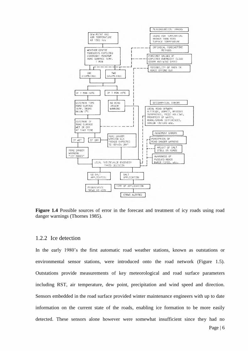
Figure 1.4 Possible sources of error in the forecast and treatment of icy roads using road
danger warnings (Thornes 1985).
1.2.2 Ice detection
In the early 1980’s the first automatic road weather stations, known as outstations or
environmental sensor stations, were introduced onto the road network (Figure 1.5).
Outstations provide measurements of key meteorological and road surface parameters
including RST, air temperature, dew point, precipitation and wind speed and direction.
Sensors embedded in the road surface provided winter maintenance engineers with up to date
information on the current state of the roads, enabling ice formation to be more easily
detected. These sensors alone however were somewhat insufficient since they had no

Page | 7
forecasting ability and were extremely localised in their measurements, to the extent that a
poorly located outstation could lead to over salting of large areas of the road network if
located in a cold spot or, more dangerously, too little salt being spread if located in a warm
spot.
Figure 1.5 A Vaisala Road Surface Analyser (ROSA) outstation monitoring road surface and
atmospheric conditions.
To resolve some of these issues a technique known as thermal mapping was developed by the
University of Birmingham and commercialised through a spin-out company Thermal
Mapping International (Thornes 1985). Thermal mapping is the process of measuring the
spatial variation of nocturnal RST along a road network (Thornes 1991). The technique is
performed using a vehicle mounted infrared thermometer which measures RST at a fixed
spatial resolution. The infrared thermometer measures the energy flux density (E) emitted by
the road surface which, according to the Stefan Boltzmann law, is proportional to the fourth
power of its absolute temperature (Liou 2002). Given the energy flux density from the
surface, RST is calculated through simple manipulation of the Stefan Boltzmann equation:

Page | 8
(1.1)
where T0 is the RST, σ is the Stefan Boltzmann constant (5.67E
-8) and ε is the emissivity of
the road surface.
As well as thermal interpolation, thermal mapping quickly became the standard method for
identifying the optimum locations for installing outstations, and for deciding the number of
outstations required to give adequate coverage of the road network. Outstations started to be
strategically located to enable the climatic variability in a particular ‘climate zone’ to be
measured. Climate zones are simply a classification of a geographical area into a series of
locations that experience a similar regional climate, such as urban centres, upland rural
regions and coastal districts (Chapman & Thornes 2006).
Originally, thermal mapping data was displayed as a thermal fingerprint (Figure 1.6) showing
RST as a pattern of temperature variations along the route (Shao et al. 1996). The amplitude
of the thermal fingerprint displays the departure of RST from an averaged value against
distance for each route (Shao et al. 1997). The extent of RST variation along a route, and thus
the amplitude of the thermal fingerprint, is controlled by atmospheric stability, with the
greatest variations being observed during stable conditions associated with anticyclonic
weather patterns (Thornes 1991). To account for these variations, thermal mapping surveys
are usually performed under a variety of synoptic weather conditions to ensure all different
levels of atmospheric stability are covered. Shao et al (1996) have shown that under a certain
weather condition the spatial variation of RST along a route appears in a consistent pattern.
This consistency enables thermal mapping surveys to be conducted under a few selected
weather conditions. In the UK, the terms extreme, intermediate and damped have been widely
used for the stability classification of thermal fingerprints, which are quantified through
analysis of the average wind speed and cloud cover during the 12-hour period preceding the
survey.

Page | 9
Figure 1.6 Thermal fingerprints showing the variation in residual (average) road surface
temperature for the same route at different levels of atmospheric stability.
Once a sample of thermal fingerprints has been collected for a particular road network,
thermal maps for each stability class are drawn up which represent the average spatial
variations of minimum RST under different weather conditions. Initially the production of
thermal maps from a combination of fingerprints was a time consuming exercise, but
nowadays with the advancements in computer processing and software, thermal maps can
-6.0
-4.0
-2.0
0.0
2.0
4.0
6.0
Re
sid
ual
RST
(°C
)
Increasing Distance
Extreme night (stable) - SD of RST = 1.35
-6.0
-4.0
-2.0
0.0
2.0
4.0
6.0
Re
sid
ual
RST
(°C
)
Increasing Distance
Intermediate night (neutral) - SD of RST = 0.80
-6.0
-4.0
-2.0
0.0
2.0
4.0
6.0
Re
sid
ual
RST
(°C
)
Increasing Distance
Damped night (unstable) - SD of RST = 0.57

Page | 10
easily be plotted in a GIS (Geographical Information System) (Figure 1.7). Based on both
thermal maps and a numerical model forecast at reference sites, the likelihood of ice or frost
forming on different parts of a road network can then be determined.
Figure 1.7 Thermally mapped data plotted in a GIS environment (Leicestershire, 10/02/08).
With the value that thermal mapping clearly added to a road weather forecast, it quickly
became the standard methodology used in most countries for thermal interpolation between
forecast sites. However, the technique is subject to a number of random and systematic errors
that are widely discussed in the road weather literature (Thornes 1991; Shao & Lister 1995;
Shao et al. 1996; Chapman & Thornes 2006) and relate largely to the repeatability of thermal
mapping surveys. Changing surface emissivity, atmospheric absorption, poor equipment

Page | 11
calibration and poor measurement of distance are just some of the sources of error that can
occur during a thermal mapping survey. A more detailed analysis of these and other errors
associated with thermal mapping can be found in Chapter 2.
1.2.3 Ice prediction
Numerical road weather prediction models were first developed during the late 1970s, but it
wasn’t until the mid-1980s that they began to be used operationally for road weather
forecasting. To provide a predictive dimension to the sensor information obtained from
outstations, a road weather prediction model based upon the zero-dimensional energy balance
approach was developed and integrated into an ice prediction strategy (Thornes 1984). The
model simulated the surface temperature and energy regime of a selected site based upon
equilibrium temperature theory, which states that if a given set of astronomical-temporal,
atmospheric and surface boundary conditions exist, there is only one surface temperature
which will balance the energy conservation equation across the surface of the earth (Outcalt
1972). The original temporal component of the model developed by Myrup (1969) was later
modified by Outcalt (1971) to produce numerical stability, convergence with available field
data and increased flexibility by increasing the number of environmental variables considered
in the model. The model was based on the energy conservation law (Equation 1.2), where the
sum of net radiation flux (Rn), latent heat flux (LE), sensible heat flux (H) and heat flux to soil
(S) is zero, i.e.,
(1.2)
At any point in time this equation must balance, and as each term is a function of surface
temperature, there is one, and only one, surface temperature that balances the equation, known
as the equilibrium surface temperature. Outcalt (1972) expanded the terms in Equation (1.2)
to further define Rn, H, LE and S as follows:

Page | 12
( )( )
(1.3)
where is the surface albedo, is beam solar radiation, is diffuse solar radiation, is
the effective emissivity of the sky (assumed to be unity), is the Stefan Boltzman constant,
is the sky temperature, is the surface temperature, and is the emissivity of the
surface.
, - (1.4)
where R is a stability correction factor (see section 4.2), C is the heat capacity of air, K is the
adiabatic estimate of the turbulent transfer coefficient whereby K = (k2U2ρ)/[ln Z2/Z0]
2 (Myrup
1969), k is von Karmen’s constant, U2 is the wind speed at air thermal damping depth of Z2, ρ
is air density, Z0 is roughness length, Z2 is the height of air thermal damping depth, T2 is the
temperature at Z2, is the dry adiabatic lapse rate, and T0 is the surface temperature.
, - (1.5)
where L is the latent heat of evaporation, q2 is the absolute humidity at Z2, and q0 is surface
wetness.
. /, - (1.6)
where Ks is the thermal conductivity of soil, Zs is the thermal damping depth of soil, and Tn is
the temperature at depth Z/2 calculated via a finite-difference solution of the Fickian diffusion
equation, whereby:

Page | 13
( ) ( ) * , ( ) ( )- ( ) + (1.7)
where I is Δt (the time increment considered), d is the thermal diffusivity and Ts is the
temperature at depth Zs.
Despite the practical difficulties in observing and interpreting the energy balance of an urban
area, numerous observational campaigns have been undertaken actively during the past three
decades, focussing mainly on the energy balance of temperate western cities (Nunez & Oke
1977; Cleugh & Oke 1986; Grimmond 1992; Grimmond & Oke 1995; Grimmond & Oke
1999a) and to a lesser extent in tropical areas, e.g. Mexico (Oke et al. 1999) and Asia
(Yoshida et al. 1991). A number of studies have shown that the geometry of urban street
canyons reduces the reflected radiant energy leaving a canyon due to multiple reflections that
occur within the canyon (Aida, 1982, cited in Offerle et al. 2007; Kondo et al. 2001; Harman
et al. 2004). Recently, research has shown that while sensible heat fluxes from roof tops
dominate daytime surface atmosphere heat exchanges, stored heat released from the urban
fabric of street canyons can help maintain neutral to unstable conditions over dense urban
areas during the nocturnal period (Christen & Vogt 2004; Grimmond et al. 2004; Salmond et
al. 2005; Offerle et al. 2006). Indeed, the representation of urban surface fluxes in energy
balance models has received great attention over the past decade in an attempt to improve
numerical weather prediction and air pollution dispersion models (Masson 2000; Best 2005;
Brown et al. 2008b). Numerical modelling and wind tunnel experiments have shown that the
differential heating of surfaces within a street canyon can influence the flow pattern, with
thermal impacts on the flow regime greatest when wind speeds are weak (Offerle et al. 2007).
Numerous simulated small-scale flows within the canopy layer (Sini et al. 1996; Baik & Kim
1999) have revealed a flow structure consisting of two counter-rotating cells caused by
heating of the windward or leeward wall, and where surface heating is introduced multiple

Page | 14
vortex development is found (Kim & Baik 2001). Hence, the overall complexity of urban
surfaces means that the energy balance shown in Equation (1.2) cannot be resolved for every
point on the urban surface, but instead requires approximation.
Thornes (1984) modified Outcalt’s model to predict RST iteratively over a 24 hour period,
based solely on the input of meteorological data. Using the twelve noon measured values of
RST and wetness along with air temperature, humidity, wind speed and cloud cover, the
model forecasted the RST and wetness for the next 24 hours, using forecast values for the
meteorological parameters at 1500, 1800, 0000, 0600 and 1200 hours. The forecast model was
run twice to produce an optimistic and pessimistic forecast, with the difference between them
giving the winter maintenance engineer a better idea of the confidence in the model (Thornes
1985). The forecast was issued in the form of a RST forecast curve (Figure 1.8), from which
early decisions could be made by the engineers regarding the treatment of the road network,
with thermal maps used to extrapolate the forecast data between outstations.
Figure 1.8 Example RST forecast curve.
-4
-2
0
2
4
6
8
10
12
14
12
:00
13
:00
14
:00
15
:00
16
:00
17
:00
18
:00
19
:00
20
:00
21
:00
22
:00
23
:00
00
:00
01
:00
02
:00
03
:00
04
:00
05
:00
06
:00
07
:00
08
:00
09
:00
10
:00
11
:00
12
:00
RST
(°C
)
Time (Hours)

Page | 15
In 1986 the Department of Transport specified the National Ice Prediction network based
around RWIS. RWIS comprise of several components which are used to predict the variation
in RST around a road network. In the original network architecture (Figure 1.9), a local
authority instation would interrogate each of the outstations along their road network via the
public switched telephone network and collect and store the measured data. This data was
then forwarded to the Met Office where it was inserted with other forecast data into their own
numerical road weather prediction model (Rayer 1987). The resulting ice prediction forecast
was sent back to the local authority instation where it was made available to the winter
maintenance engineer to aid them in their decision making.

Page | 16
Figure 1.9 Schematic of the National Ice Prediction Network (Rayer 1987).
In 1988 the architecture of the UK National Ice Prediction network changed somewhat with
the development of a central bureau service for data collection and archiving. With the bureau
service, local authorities were no longer responsible for interrogating their outstations, as this
was all controlled centrally from within the bureau. Once collected, data was validated before
being sent to a forecast provider to be inserted into a road weather prediction model. The
resulting forecast was then sent to the bureau where it was disseminated to the relevant local
authority winter maintenance engineer. This bureau structure is still in use today, although
Numerical model
Model output
Model input
Met Office weather
centre Local authority
highways maintenance
Sends ice
prediction
Road Sensor Roadside
Equipment
Local authority
‘outstation’
Road Sensor Roadside
Equipment
Local authority
‘outstation’
Local authority
‘instation’
Requests sensor
readings Requests sensor readings and ice
prediction
Interrogates outstations and stores
sensor readings, and ice prediction

Page | 17
technological advancements have helped to improve efficiency and reduce costs. For
example, mobile GSM and GPRS communications are increasingly being utilised to transfer
outstation data to a central bureau, and with advancements in solar power technology the
outstations themselves can now be located in more remote locations where mains power is
unavailable, thus increasing coverage around the road network. Perhaps the most noticeable
advancement however is the increasing efficiency with which forecasts are now disseminated
to the winter maintenance engineer. With the use of web servers for hosting forecast and
sensor data, dissemination of this data has become an automated process and winter
maintenance engineers now have access to forecast and actual sensor data 24 hours and day
during the winter season via the internet.
Numerical prediction of ice and frost has been accepted by both winter maintenance engineers
and meteorologists as an appropriate and valuable technique for winter road maintenance.
Road weather models provide winter maintenance engineers with advance knowledge of
where and when ice or frost is likely to occur, enabling them to better plan salting strategies.
The technique enables highway authorities to maintain or improve already established road
safety standards, whilst also reducing the huge costs associated with salt usage, labour and
equipment, and the damage caused to the environment (Shao & Lister 1996). A survey in the
mid-1990’s commissioned by the UK Met Office found that approximately £170 million and
up to 50 lives have been saved each year in the UK since the introduction of a road ice
prediction system (Thornes, 1994).
The last decade of the twentieth century saw a great deal of research focused towards
improving the accuracy of road weather prediction models, much of which was prompted by
the rapid increase in the processing capabilities of computers. In the early 1990’s there were
two road weather models in commercial use in the UK: the Met Office Road Surface
Temperature model (MORST) (Rayer 1987; Thompson 1988), and Vaisala’s ICEBREAK
model (Shao 1990), both of which have undergone continuous developments as the

Page | 18
processing capabilities of computers has increased. Data input into the MORST model was
streamlined with the inclusion of a mesoscale model, which provided the benefit of being less
pessimistic than the numerical equivalent, thus reducing model bias (Astbury 1996). The
coarse scale of the model however caused problems since interpolation of the data for forcing
the RST model could lead to errors in representivity (Maisey et al. 2000). For example,
smaller topographical variables were sometimes disregarded, and grid-points of the mesoscale
model did not always coincide with the outstation sites used by the original model (Thornes &
Shao 1992). To overcome this, Thornes & Shao (1992) recommended linearly combining
grid-points to provide a better data input set together with an averaging template of several
days to correct for systematic error. With the obvious inadequacies of the mesoscale model in
driving the MORST model, in the mid to late 1990’s the Met Office developed a high
resolution Site Specific Forecast Model which uses high resolution (25 metre horizontal) land
use data to estimate localised surface fluxes, the incorporation of which has shown significant
improvements over the mesoscale model for site specific forecasting and helped to improve
road weather forecasts internationally (Maisey et al. 2000).
The ICEBREAK model has also been continuously developed to the point where it is now
fully automated and can be used for three hourly nowcasting, with no external meteorological
input data required other than automatically collected sensor measurements of RST, air
temperature, dew point and wind speed from the forecast site (Shao & Lister 1996). The
application of a three-layer neural network trained by an error-back propagation algorithm has
further increased the accuracy of nowcasts by reducing the root mean square error (RMSE) of
temperature forecasts and increasing the accuracy of frost-ice prediction, particularly at
problematic sites where complex environmental conditions and underlying nonlinear
mechanisms are unresovlable by operational numerical models (Shao 1998).
In 1997 PA Weather Centre (now MeteoGroup UK), a joint venture between the Press
Association and Dutch weather forecasting company Meteo Consult, was established and

Page | 19
started supplying forecasts to a wide range of clients including some in the road industry. The
Press Association road forecast model has since been developed to produce site forecast
graphs using a statistical approach in combination with traditional energy balance equations
(http://www.meteogroup.co.uk/).
A number of other models remain in development around the world, most notably the RWFS
(Road Weather Forecast System) in the US which was developed as part of a five year
Federal Highway Administration (FHWA) program, initiated in 1999, to explore the
applicability of technologies developed at national research laboratories to the problem of
winter road maintenance (Schultz 2005). The first specific goal was to develop an automated
decision support system to generate snow ploughing and roadway chemical application
guidance for use by state departments of transport, which led to the development of the
Maintenance Decision Support System (MDSS) (Mahoney et al. 2005). In the MDSS
prototype architecture, the gridded outputs from an ensemble of mesoscale model forecasts
generated by the National Oceanic and Atmospheric Administration’s Forecast Systems
Laboratory (FSL) are transmitted in real time to the Research Applications Laboratory at the
National Centre for Atmospheric Research. Here, the FSL models are ingested along with a
large scale lateral boundary model into the RWFS, where they are combined with a Road
Condition and Treatment Model (RCTM) which is the central component of the MDSS. The
function of the RCTM is to produce road condition forecasts and treatment recommendations
(Petty & Mahoney 2008), using the Model of the Environment and Temperature of the Roads
(METRo) (Crevier & Delage 2001; Linden & Drobot 2010) to generate predictions of
pavement conditions, with treatment recommendations constructed using current and
forecasted atmospheric and road condition information (Petty & Mahoney 2008).
A restriction of all the road weather models discussed thus far is that they only produce RST
forecasts for the outstations from which meteorological data are obtained, with thermal
mapping required to extrapolate this forecast data around a road network. Alternative methods

Page | 20
to thermal mapping have been proposed, most notably the use of empirical local
climatological and statistical models to predict spatial variations of RST in a road network
(Bogren et al. 1992; Gustavsson & Bogren 1993). Such models are in commercial use in
Sweden and have helped to demonstrate the influence of geographical factors (Bogren &
Gustavsson 1991; Bogren et al. 2000a) and meteorological parameters (Gustavsson et al.
1998; Bogren et al. 2000b) on RST. However, local statistical models require a large number
of observations to obtain reliable statistical relationships, and any such model derived in one
area will usually require major modification before it can be applied to another area (Shao et
al. 1997). With such doubts on the accuracy and general applicability of statistics-based
climatological models, thermal mapping has until recently remained the standard
methodology used in most countries for describing and displaying variations in RST between
forecast sites.
This first generation of RWIS described thus far relies largely on methods and tools
developed in the 1980s, but as technology has progressed and the processing capabilities of
computers has increased, it is now being superseded by a new generation of RWIS capable of
forecasting for individual salting routes, rather than traditional site specific forecasts which
rely on interpolation by thermal mapping.
1.2.4 Route-based forecasting
Within a climate zone there usually exists at least one outstation, and the weather recorded at
this outstation is assumed to be representative of the climate zone as a whole. Chapman &
Thornes (2001a; 2001b) use this assumption to hypothesise that if the regional climate is
constant, any variation in climate and RST across the climate zone is controlled by the
variation in geographical parameters. They further suggest that by measuring local variations
in geography and modelling the impact of these variations on RST, accurate ‘virtual’ forecasts
can be created away from the road weather outstation, thus enabling route-based forecasts to

Page | 21
be produced. Such an approach enables the thermal projection of RST across the road network
entirely by model predictions without the need for thermal maps.
Chapman et al. (2001b) developed an improved road weather prediction model (ENTICE)
based around the Thornes (1984) model, with an added high resolution, site-specific spatial
component to predict local variations in RST over both time and space. The spatial
component of ENTICE is driven by a Geographical Parameter Database (GPD) consisting of
several geographical parameters that have been widely proven to influence RST. In a pilot
study in the West Midlands, UK, ENTICE was shown to be able to explain up to 72% of the
variation in RST purely by thermally projecting surface temperature using geographical
variables (Chapman et al. 2001b). A later study by Chapman & Thornes (2006), again in the
West Midlands, found that ENTICE could explain up to 74% of the variation in RST in urban
areas and up to 58% in rural areas.
The ability to thermally project RST across a road network entirely by model predictions
raises the question of whether thermal mapping is still a required component of RWIS. The
requirement of thermal mapping as a forecasting tool has diminished as the predictive ability
of numerical models has improved, and this is likely to continue as more local authorities start
to use route-based forecasting solutions within their winter maintenance strategies. However,
the development of route-based forecasting has brought with it a new challenge relating to the
validation of the forecasts – How can a route-based forecast be validated? Whilst traditional
site specific forecasts can be validated against sensor data from outstations located at the
forecast sites, no such data exists for verifying the thermal projections of RST between
outstation locations in a route-based forecast. Chapman et al. (2001b) and Chapman &
Thornes (2006) used data acquired from thermal mapping surveys as a means of testing the
predictive ability of the ENTICE route-based forecasting model, which suggests that the
future role of thermal mapping within the framework of route-based forecasting could be that
of a validation tool. However, whilst the results obtained using thermal mapping data to

Page | 22
validate the ENTICE model were generally good (up to 74% of thermal variations around the
route explained by the model), these results were based on average statistics for an entire
study route and provide no indication of the variation in model performance around the route.
Hence, the current methodology of using ‘entire route’ statistics obtained from the averaging
of thermal mapping data is clearly too simplistic and needs to be changed. The increased
resolution of route-based RST forecasts requires validation at a whole new spatial scale that
up until now has never been required for road weather forecasts. Clearly route-based
forecasting is a significant step forward, but it is still a relatively new concept to some local
authorities, many of whom do not yet have the confidence to be able to selectively salt their
road network based solely on model predictions. In order to build this confidence, more
attention needs to be focused towards improving the validation strategy for route-based
forecasts, which possibly represents one of the biggest challenges currently facing the road
weather research community.

Page | 23
1.3 Aims and Objectives
1.3.1 Aims
This thesis has two main aims. The first of these is to develop the foundations for a new
validation strategy for route-based road weather forecasts that will potentially enable
validation at the full spatial and temporal resolution of the model. Such a technique must be
capable of identifying variations in spatial model performance to enable weaknesses in the
forecast model to be more easily identified and resolved. Moreover, it is intended that the new
validation strategy be used as a consistent methodology for identifying whether new model
parameterisations (whenever proposed) improve the overall spatial forecasting performance
compared to existing parameterisations. Since ENTICE assumes that the local geography and
road infrastructure are the main influence on thermal variations within a climate zone, it is
imperative that we also get better control over the geographical and infrastructure parameters
that are currently inadequately parameterised in the model. Hence, the second aim of the
thesis is to improve the accuracy of the ENTICE route-based forecast model by de-
parameterising key geographical and infrastructure parameters within the model that are
currently not measured at the spatial scale demanded by a route-based forecast.
1.3.2 Objectives
These aims will be achieved through the following objectives:
1. To critically review existing road weather validation techniques as tools for verifying
route-based road weather forecasts.
2. From the outcome of (1), devise a new methodology to facilitate validation of the
ENTICE model at a spatial scale previously unseen with route-based forecasts.
3. Investigate new techniques to remove geographical and infrastructure parameterisations
in the ENTICE model, namely:

Page | 24
i. Road construction re-parameterisation through the use of Ground Penetrating
Radar technology.
ii. Surface roughness (land use) re-parameterisation using airborne LIDAR data.
4. To use the validation strategy devised in (2) as a new methodology for testing whether
the changes to geographical and infrastructure parameterisation improve the overall
spatial forecasting performance of the ENTICE model.
5. Make recommendations for the future of route-based forecasting
The road weather market in the UK is currently in a transition phase with an increasing
number of local authorities changing to a route-based forecasting system, and it is hoped that
the results of this thesis will have a positive impact on a number of different fronts. Increased
model performance will help to increase overall confidence in route-based forecasting, which
is crucial if local authorities are ever to adopt selective salting strategies that require the
confidence to simply treat one section of road and risk leaving another warmer section
untreated. Economically, the realisation of selective salting should bring huge financial
savings to local authorities as the efficiency of winter maintenance operations improves, and
with increased confidence in the model local authorities should also be more receptive to the
idea of optimising their salting routes (Handa et al. 2007), a strategy which offers the potential
for even greater financial savings. Furthermore, increased forecast accuracy should lead to
better treatment decisions which will ultimately help to reduce the number of weather-related
road traffic accidents that occur each year. From an environmental perspective, improvements
to route-based forecast accuracy will ultimately result in smaller quantities of de-icing
material being required to treat road networks, reducing the levels of salt and associated
additives entering water courses via road runoff. Finally, from a modelling perspective,
although this research is being conducted using the ENTICE route-based forecast model, the

Page | 25
validation strategy and any newly proposed model parameterisations will be relevant to any
spatial road weather model.
CHAPTER ONE SUMMARY
The development of route-based road weather models was the first real innovation in road
weather forecasting in over a decade and was long overdue. The technique of route-based
forecasting enables the thermal projection of RST around a road network at a high spatial
resolution entirely by model predictions. However, the increased resolution of route-based
forecasts requires validation at a whole new spatial scale that up until now has never been
required for road weather forecasts. The improved spatial scale of route-based forecasts also
places an increasing demand on measurement requirements in order to fully account for the
variations in geographical and infrastructure parameters which influence thermal variations
around a route, some of which are not currently measured at the spatial scale demanded by a
route-based forecast. This thesis aims to address these issues, starting with the development a
new validation strategy in the following chapter.

Page | 26
2. A NEW VALIDATION STRATEGY FOR ROUTE-
BASED ROAD WEATHER FORECASTS
The road weather industry is becoming an increasingly commercial environment, and users of
road weather forecasts are continually having to prove that they are getting value for money
from their winter maintenance expenditure (Thornes & Stephenson 2001). The quality and/or
value of weather forecasts has received much attention in the literature (Mylne 1999; Thornes
1995; Thornes & Proctor 1999; Stephenson 2000), and as route-based forecasting techniques
have led to significant increases in the spatial resolution of road weather forecasts, model
validation along the entire length of a route is now a real necessity. Validation loosely refers
to the process of assessing whether a design, procedure or process is correct and satisfies
specified requirements (Edwards et al. 2002). The traditional methods of validation for road
weather forecasting, which are discussed in the following section, no longer satisfy the
increased spatial demands of route based forecasts, and as will become apparent through the
remainder of this chapter, the aim of this part of the research is to develop a streamlined
methodology for calculating route-based model performance at a much greater spatial
resolution than is currently feasible, hence improving route-based forecast model validation.
2.1 Existing Validation Techniques
2.1.1 Road outstations
Since the development of ice prediction strategies in the mid-1980s, road weather outstations
have provided the main source of validation data for site specific forecasts produced by road
weather prediction models. However, with the emergence of route-based forecasting as the
standard methodology for delivering winter maintenance services in the UK, the limitations of
road outstation data are becoming increasingly apparent. Even with careful design and

Page | 27
installation and assuming good sensor calibration, embedded road sensors only provide a spot
measurement of RST and are therefore unable to provide information on the spatial variation
of RST around a road network. This severely limits their use as a validation tool for route-
based forecasts, although instances occur where spot measurements of RST could provide
useful information. In the UK, road outstations are strategically located to enable climatic
variability to be measured, but some countries take a more pessimistic approach and
specifically locate outstations at the coldest locations around a road network to give a ‘worst
case’ scenario. Cold spots or thermal singularities such as frost hollows and bridge decks are
some of the most difficult locations for road weather models to resolve (Shao 1998), and
outstations located at these problematic sites could provide useful spot measurements for
validation in a route-based forecast model. However, in countries such as the UK outstations
are rarely located at such problematic sites, and to do so now would require large amounts of
investment that few highway authorities can afford given the large costs of installing new
road outstations and the continual pressures winter maintenance managers face to reduce
expenditure. A more realistic alternative could involve the installation of low cost remote
infrared temperature sensors for monitoring RST at problematic forecast sites that are
recognised thermal singularities.
2.1.2 Remote infrared temperature sensors
Recently developed remote infrared surface temperature sensors from established instrument
manufacturers such as Vaisala (Cyclo) and Campbell Scientific (IRIS; Figure 2.1) provide
low cost alternatives to traditional road outstations and have a number of advantages over
their predecessors that facilitates their use as a validation tool. Such sensors utilise modern
solar power technology and remote GSM/GPRS communications which significantly reduces
installation costs as no fixed power and communication lines are required. Whilst many
traditional outstations are now equipped with mobile communications, their locations are
generally restricted to sites with mains power due to the high power consumption of

Page | 28
embedded surface sensors and an increasing demand for outstation cameras capable of live
video streaming over IP networks. This gives low power remote infrared sensors a distinct
advantage for route-based forecast validation since a much greater network coverage is
possible, making it feasible to install one or more sensors on every forecast route at a
reasonably low cost. These sensors also have the added advantage of measuring RST over a
larger surface area compared to the spot measurements of embedded surface sensors, making
them less susceptible to erroneous measurements and providing a more realistic indication of
the average RST at a particular site.
Figure 2.1 An IRIS remote infrared temperature sensor monitoring road surface temperatures
at the Eurotunnel freight terminal in Folkestone, UK. Photograph courtesy of Campbell
Scientific Ltd.

Page | 29
Remote infrared sensors can be susceptible to measurement errors due to traffic, however, and
whilst sensors have traffic filtering algorithms programmed into the systems, the effectiveness
of these algorithms under heavy traffic conditions is somewhat unknown and requires further
study. Furthermore, these sensors contain algorithms to account for the increased effects of
atmospheric radiation on RST under clear sky conditions when other infrared sensors are
often inaccurate, but these algorithms contain certain assumptions that can sometimes lead to
measurement errors since neither sensor directly measures the actual sky temperature for
inclusion into its algorithms. Surface emissivity is another potential source of error for remote
infrared sensors. Emissivity is defined as ‘the ratio of the total radiant energy emitted per unit
time per unit area of a surface at a specified wavelength and temperature to that of a
blackbody under the same conditions’ (Oke 1992). Tabulated values give an emissivity for
concrete of 0.92-0.94 and 0.967 for asphalt, but the apparent emissivity of a road surface will
vary according to surface state and the view angle of the sensor (Gustavsson 1999). Remote
infrared sensors are usually pre-calibrated for specific surface types based on tabulated
emissivity values, but any changes to the apparent emissivity are not accounted for and will
affect the accuracy of temperature readings.
Despite these potential errors, an increasing number of highway authorities around the world
are using remote infrared sensors as a low cost alternative to increase coverage of their road
network between existing road outstation locations, mainly attracted by the lower purchase
and installation costs and the greater network coverage that these sensors offer. However, as
with traditional road outstations, remote infrared sensors are unable to provide information on
the spatial variation of RST around a road network, and although their low cost provides an
opportunity to instrument the network at a greater resolution, this will still be significantly
coarser than the forecast points used in a route-based forecasting service. Ultimately, this
would require thousands of infrared sensors to be installed around the road network which is
clearly impractical. As a validation tool for problematic forecast sites around salting routes

Page | 30
however, remote infrared sensors have several benefits over traditional outstations, and could
potentially be used for verifying specific forecast points around a route.
2.1.3 Thermal mapping
Whilst road outstations and remote infrared sensors are unable to verify the spatial variation
of RST around a road network, one existing technique does fulfil this requirement. The
technique of thermal mapping has been used in applied road climatological studies since the
mid-1970s, but it wasn’t until the mid-1980s that the use of thermal mapping became
common practice in winter road maintenance. The technique played a key role in the
progression from basic ice detection systems to ice prediction, and more than 20 years on the
same technique could have an equally important role to play in the progression from climatic
domain to route-based forecasts. Thermally mapping the road network with a vehicle mounted
infrared temperature sensor provides a data set describing the spatial variation of RST around
the road network (Shao et al. 1997), precisely what is required for verifying a route-based
forecast. It is well documented that the technique of thermal mapping is subject to a number
of random and systematic errors (Table 2.1), but under strict quality control many of the
errors can be minimised or eliminated altogether. For example, distance errors due to
differences in tyre pressures, cornering at different angles and variations in speedometer
accuracy between vehicles have now been eradicated by fixing the exact location of each
reading with GPS (Chapman et al. 2001a). Other errors, however, are less easy to resolve, and
Table 2.1 provides a summary of the main errors currently associated with thermal mapping.
These are divided into two types of error. The first of these is random errors that are caused
by unknown and unpredictable changes in the measurement, which are changes that may
occur in the measuring equipment or in the environmental conditions. The second type of
error is systematic errors caused by the measuring equipment, which usually result in some
form of bias in the sensor measurements rather than a random fluctuation.

Page | 31
Table 2.1 Potential sources of error in thermal mapping (adapted from Thornes (1991) and
Chapman et al. (2005).
Random errors due to unknown and
unpredictable changes
Systematic errors from the measuring
equipment
Varying road surface emissivity Temperature range of instrument exceeded
Atmospheric absorption & attenuation Contaminated optics
Signal noise Sensor angle
Narrow sensor waveband Variations between sensors due to tolerance
Lane changes due to slow moving vehicles
Unstable sensor body temperature
The greatest source of random error during a thermal mapping survey is the emissivity of the
road surface, which will vary according to the road surface material and, to a lesser extent,
road surface state. Despite these variations, for the purposes of thermal mapping surface
emissivity is typically held constant at 0.95 (Sugrue 1983). Road surface temperatures
calculated from the surface energy flux density (E) using the Stefan-Boltzmann law are
extremely sensitive to even the smallest change in emissivity. Gustavsson (1999) estimates
that a 10% change in emissivity from 0.95 to 0.85 will cause an infrared detector to under
read surface temperature by approximately 8°C when E = 300 Wm-2
. Thornes (1991) puts this
temperature difference at a more conservative 5°C, which given the variation in emissivity
between concrete and asphalt surfaces of up to 4% can lead to a potential error around a
survey route of approximately ±2°C. Another important parameter affecting surface
emissivity is road surface state. Measurements using an infrared sensor have shown that
calculated RST on an asphalt surface can vary by approximately 0.8°C depending on whether
the surface is dry or moist (Gustavsson 1999), which restricts the periods over which thermal
mapping surveys can be conducted to situations with constant surface status, otherwise it can

Page | 32
be difficult to interpret the temperature recordings collected. Atmospheric absorption is
another potential source of random error in thermal mapping (Thornes 1991), preventing all
of the radiation from the surface reaching the sensor. However, well designed infrared sensors
are sensitive to a specific waveband between 8 and 14 µm known as the atmospheric window
(Liou 2002), where radiation from the Earth is almost completely reflected with little
atmospheric attenuation, so errors due to absorption should be minimal with a well-designed
sensor and can be further avoided by positioning the sensor close to the road surface.
Alongside this, good calibration is required to compensate for the narrow waveband of most
infrared sensors which only transmit part of the infrared spectrum, and even more desirable is
individual sensor calibration, which will also eradicate random errors between sensors due to
component tolerances.
A further source of random error in thermal mapping, and one which can easily be
overlooked, is that caused by an unstable sensor body temperature. Modern infrared sensors
utilise a thermopile detector which detects the presence of thermal radiation, consisting of a
number of thermocouples connected in series. One set of thermocouple junctions is exposed
to the radiation source (i.e. the road surface in the case of thermal mapping) and is heated by
it, whilst the other set is shielded from the radiation. A highly polished metal cone
concentrates the radiation onto the exposed junctions, which are coated with lamp-black to
enhance the efficiency with which the radiation is absorbed. The output from the thermopile
detector is a voltage proportional to the thermal energy balance between itself and the surface
it is detecting. Taking Equation 2.1, the rate at which a unit surface area of a road surface
receives radiation from surrounding objects at temperature T0 is σT04, and the net rate of loss
of energy by the road surface is given by Inet, as shown in Equation 2.1:
4
0
4 TTI net (2.1)

Page | 33
where T is the surface temperature observed by the detector and T0 the temperature of the
detector usually measured by an internal thermistor (Liou 2002).
The voltage output by the infrared sensor is proportional to this thermal energy balance, so the
maintenance of a stable body temperature is essential for accurate measurements to be made.
In addition, infrared sensors are calibrated in such a way that increased accuracy is achieved
with smaller temperature differences between the sensor and the target surface. As such, the
positioning of an infrared sensor on a vehicle should be carefully considered to minimise
random errors relating to the thermal energy balance, and systematic errors such as signal
noise from vehicle emitted radiation or contaminated sensor optics due to dirt and
condensation. The angle at which the sensor is mounted on the vehicle is also important since
it will influence how much radiation received by the sensor originates from the road surface
and how much comes from surrounding objects and the atmosphere (Gustavsson 1999). To
minimise the influence of surrounding objects and the atmosphere, the infrared sensor should
be mounted in a nadir position. In addition, apparent emissivity has been shown to change
with view angle (Scott 1986; Lagourade et al. 1995), with detailed studies over an asphalt
surface showing an 8% decrease in apparent emissivity with a view angle of 45° (Bergendahl
1998 cited in Gustavsson 1999). However, this variation is much greater than those found in
other studies, and Gustavsson (1999) suggests further work is required in this area to
understand fully the effects of varying view angle on RST.
The use of thermal mapping as a validation tool for route-based forecasts is by no means a
new idea. The technique was first used for such purposes by Chapman et al. (2001a; 2001b),
and Weather Services International have successfully used the technique to verify their
OpenRoute™ route-based forecasting service, driven by the ENTICE model, during the
2006/07 and 2007/08 winter seasons (White 2007). In its current form however, thermal
mapping is a time consuming and costly exercise. The large extent of some highway authority
road networks means that a single complete survey covering all salting routes can often take

Page | 34
several nights to complete given the time restrictions imposed on surveys by daylight and
traffic loads. Research has shown that traffic is a major source of potential error in thermal
mapping surveys (Prusa et al. 2002; Chapman & Thornes 2005), with heat fluxes from
vehicles having the effect of increasing RST which consequently impacts on the timing of
thermal mapping runs. Chapman & Thornes (2005) suggest limiting thermal mapping surveys
to the few hours before sunrise on weekends to avoid ‘snapshot’ data collected at any other
time which they argue will not be representative of minimum temperatures. Whilst this may
be a somewhat histrionic approach, it emphasises the fact that thermal mapping surveys are
restricted to a small time window, during which it is impossible to survey the full spatial and
temporal resolution of a route-based forecast. This somewhat limits the usefulness of thermal
mapping as a suitable long term validation technique for route-based forecasts. Given the time
constraints associated with thermal mapping surveys and the growing demand for validation
data as increasing numbers of highway authorities use route-based forecasting services, the
time appears to have come for a new validation technique to be developed. Any new
technique will need to be both robust and reliable, whilst at the same time offering a rapid and
cost effective solution for the forecast provider, but unless a new technique allowing
validation at the full spatial and temporal resolution can be found, compromises will have to
be made.
2.2 Data Reduction
From the review of existing validation techniques, it is clear that no one technique provides
the answer to verifying a route-based forecast. Clearly validation cannot be achieved using
regression analysis on thermal mapping data since the aim is to verify rather than predict
RST, with the latter undertaken using heat balance models. The main problem is the vast
number of points that need to be validated, and a sensible approach is somehow to reduce the
number of points needing to be validated to provide a more manageable dataset. An obvious

Page | 35
solution would be simply to reduce the resolution of the route-based forecast, say from 50
metres to 100 metres. This would immediately halve the number of forecast points needing to
be validated, but would bring no operational benefit to the forecast provider since it would
still require the same mileage of road network to be driven for thermal mapping validation.
Additionally, any reduction in the resolution of the route-based forecast can be seen as a
reduction in the quality of the forecast since it reduces the ability to be able to identify and
model small scale thermal singularities around the road network such as bridges and areas
prone to katabatic drainage. In an environment of increasing litigation there is an argument to
be made that even a resolution of 50 m is insufficient since RST has been shown to vary by
over 1.5°C at the sub-metre scale (Chapman & Thornes 2008). Clearly an alternative
methodology is required in order to reduce the number of points needing to be validated
without compromising on the quality of the route-based forecast being delivered.
2.2.1 Techniques for data reduction
Numerous statistical techniques are available for the purposes of data reduction, and many of
these can be categorised under the general headings of Factor Analysis or Clustering. The
most common form of Factor Analysis for achieving data reduction uses principal
components extraction and is commonly referred to as Principal Components Analysis (PCA).
The central idea of PCA is to describe a dataset consisting of a large number of variables by
means of only a few variables, while retaining as much of the variability present in the
original dataset as possible (Preisendorfer 1988). PCA is commonly used in the field of
geographical sciences where an abundance of instrumentation often enables numerous system
variables to be measured and large sample sizes to be collected. When more than two or three
variables are being measured, it can often become difficult to visualise their relationships.
However, in data sets with many variables, groups of variables are often associated and co-
vary together, since more than one variable might be measuring the same driving principle

Page | 36
1 2 3 4 5 6 70
10
20
30
40
50
60
70
80
90
100
Principal Component
Variance E
xpla
ined (
%)
0%
10%
20%
30%
40%
50%
60%
70%
80%
90%
100%
governing the behaviour of the system. In many systems there are only a few such driving
forces, even though an abundance of instrumentation enables you to measure many system
variables. PCA is a quantitatively rigorous method of simplifying a dataset by replacing a
group of variables with a new set of variables (axes) called principal components, each treated
as a single axis in space. Each principal component is a linear combination of the original
variables, but all the components are orthogonal to each other so are uncorrelated. The full set
of principal components explains all of the variance in the original set of variables.
Figure 2.2 Example Pareto chart for showing the variance explained by each principal
component.
The percentage of variance explained by each principal component is best viewed using a
Pareto chart (Figure 2.2) where the principal components are arranged and plotted in
descending order, with an accompanying line graph showing the accumulative variance. The
first principal component accounts for as much of the total variance in the dataset as possible,
with the second principal component accounting for as much of the remaining variance as

Page | 37
possible whilst being uncorrelated with the first component, continuing in this way until there
are as many components as original variables. It is commonplace for the sum of the variances
of the first few principal components to explain the majority of the total variance of the
original data, with the remaining components accounting for only a small part of the total
variance and thus being unimportant. By examining plots of the main principal components of
a dataset it is possible to identify the dominant patterns of spatial variability in the data to
develop a deeper understanding of the driving forces that generated the original data.
Clustering can most easily be defined as the grouping of similar objects using data from the
objects (Seber 2004). It is a general term which encompasses a number of different algorithms
and methods for organising datasets into groups in such a way that the degree of association
between two objects is greatest if they belong to the same group and minimal otherwise. The
goals of cluster analysis are varied and include widely different activities such as hypothesis
generation, identification of ‘natural’ groups of like objects to form the first stage of a
stratified sampling strategy, and the development of classification schemes such as the
classification of plants and animals (taxonomy) or diseases (Seber 2004). Clustering
techniques have been applied to a wide variety of research problems in numerous subject
areas including archaeology, anthropology, agriculture, economics, education, geography,
geology, linguistics, market research, genetics, medicine, psychology, psychiatry and
sociology, and Hartigan (1975) provides an extensive summary of numerous published
studies reporting the results of cluster analyses.
Seber (2004) identifies three main types of clustering: Hierarchical clustering, Partitioning
and Overlapping clusters. In hierarchical clustering the clusters are themselves grouped into
other clusters, with the process being repeated at different levels to form a tree of clusters
often referred to as a dendrogram. The cluster tree can be constructed using either a bottom-
up agglomerative approach involving a series of successive fusions of n objects into clusters,
or from the top down using a divisive method which partitions the total set of n objects into

Page | 38
increasingly smaller clusters (Seber 2004). Within partitioning methods of clustering, objects
are partitioned into non-overlapping clusters, the number of which is usually determined in
advance. Although there are numerous partitioning methods of clustering, K-means is perhaps
the most commonly used. The K-means analysis procedure assigns objects to clusters based
on distance from pre-assigned cluster centres, the locations of which are updated based on the
mean values of the objects in each cluster. Overlapping clusters, sometimes referred to as
Clumping, are rarely used and intended for situations where it is more meaningful to allow a
certain degree of overlap between clusters (Seber 2004). Such an example would be in
linguistics, where words can have several meanings and may belong to several groups.
Overlapping methods of clustering, however, are generally more computationally complex
and the results more difficult to interpret (Sneath & Sokal 1973), leaving hierarchical and
partitioning methods of clustering as the preferred options for multivariate analysis.
2.2.2 Data reduction in the ENTICE route-based forecast model
2.2.2.1 Building the ENTICE GPD
The spatial modelling approach used in the ENTICE route-based forecast model is driven by a
GPD consisting of several geographical and infrastructure parameters listed in Table 2.2.
Construction of the ENTICE GPD firstly requires View Factor Mapping (VFM) surveys to be
undertaken, where sky view factor (ψs) data are collected in real-time using a patented method
first developed by Chapman & Thornes (2004). This technique uses a feed-forward back-
propagation artificial neural network to calculate ψs by proxy by measuring the number of
tracked and visible satellites in the Global Positioning System (GPS) network and the quality
of incoming signal to noise ratios from the satellites. The equipment used in a VFM survey
consists of a Navman GPS development unit with a roof mounted antenna connected to a
laptop computer via USB connection, both powered from a 12V DC in-car cigarette lighter
via a 12V DC to 230V AC 150W power invertor. Bespoke logging software is used to initiate

Page | 39
the logging of GPS positional and proxy ψs data which is automatically appended to a
database file every second. With the positional and ψs data being logged, a survey route is
driven and to ensure optimum GPS positional fix throughout the survey, driving speed along
the route is restricted to a maximum of 50 mph.
Table 2.2 Meteorological, geographical and road infrastructure parameters used to drive the
ENTICE road weather prediction model (Chapman et al. 2001a).
Meteorological Parameters Geographical Parameters Road Parameters
Solar radiation Latitude Depth of construction
Terrestrial radiation Altitude Thermal conductivity
Air temperature Topography Thermal diffusivity
Cloud cover and type Screening Emissivity
Wind speed Sky View Factor (ψs) Albedo
Humidity / dew-point Landuse Traffic
Precipitation Topographic exposure
Altitude, slope and aspect data for each forecast point are obtained from a high resolution
digital elevation model (DEM) using GIS software, and road type data are derived from
Ordnance Survey®
Meridian™
data. A proxy classification of land use density is obtained via
a spatial density analysis of vector road data using the method described by Chapman &
Thornes (2006) to locate dense areas of the road network, with the assumption that more
heavily urbanised areas have a denser road network than suburban and rural areas. Traffic
density is parameterised through use of a general traffic algorithm (Chapter 6) described by
Chapman (2002) that introduces a slight temperature bias dependent on land use and road
type classifications and a shadowing coefficient to account for reduced outgoing long-wave
radiation from the road surface caused by vehicles. The treatment of traffic in this way is
simplistic and could be greatly improved by consideration of daily traffic densities from
sources such as Motorway Incident Detection and Automatic Signalling (MIDAS) loops, but

Page | 40
such data is not freely available in the UK, thus hindering the development of an accurate
traffic coefficient. An alternative methodology could potentially involve the use of raw data
from remote infrared temperature sensors which use traffic filtering algorithms to remove
most of the noise associated with passing vehicles, and this would enable greater network
coverage than MIDAS loops that are typically only installed on motorways and the most
heavily congested A-roads.
2.2.2.2 Birmingham study route
Figure 2.3 displays a mixed urban and rural study route in Birmingham, UK, which was
selected as a test bed for this research. The study route, which traverses through Birmingham
city centre before passing through the south-west Birmingham suburbs and north
Worcestershire countryside, was chosen for this study due to the large variation in geography
around the route and also due to the large amount of thermal mapping data that exists for the
route. Figure 2.4 (a) to (d) display elements of the ENTICE GPD for this study route plotted
as a series of layers in a GIS to show the variation of geographical and road infrastructure
parameters around the route. Altitude around the study route varies from between 120 m in
the suburbs of Birmingham up to 250 m in the rural Clent Hills to the south-west of the route
(Figure 2.4 (a)). Variations in land use and road type are clearly identifiable in Figure 2.4 (b)
and (c), ranging from A-roads in the heavily urbanised city centre to more minor roads in the
rural and semi-rural areas of the route. The variation in ψs around the route (Figure 2.4 (d)) is
as expected, with ψs values generally lower in the city centre and higher in rural areas,
although exceptions to this rule include some rural tree lined roads and locations underneath
bridges and underpasses which have very low ψs values.

Page | 41
Figure 2.3 Map displaying the mixed urban and rural study route in Birmingham, UK, which
was used as the test bed for the research in this thesis.

Page | 42
Figure 2.4 Geographical and infrastructure parameters from the ENTICE GPD plotted as
layers in a GIS, showing variations in geographical and infrastructure parameters around the
Birmingham study route for (a) altitude; (b) land use; (c) road type; (d) ψs.
2.2.2.3 Modifications to the ENTICE GPD
Modifications were required to some of the data within the GPD before data reduction could
occur. For example, the ordinal nature of land use and road type data creates problems for
clustering algorithms since the distance between two objects in an ordinal dataset may bear no
relation to the similarity or dissimilarity between the objects, and could have a negative effect

Page | 43
on the clustering solution. To overcome this issue, average thermal conductivity values for the
road surface at each forecast point were calculated based on the assumption of a five zone
flexible pavement identical to that used by Chapman (2002), with variations in the materials
and hence thermal properties of each zone according to the road type classification (see
Chapter 3 for further details). Similarly, ordinal land use data was replaced with roughness
length (Z0) values similar to those used by Chapman (2002) which vary with respect to both
the land use and road type classifications and are based on Z0 values assimilated from
scientific literature. Whilst these new variables still contain categorical data which it is
recognised can reduce the objectivity of distance measures in clustering algorithms, numerous
studies have shown that both land use and road construction can have a significant influence
on RST (Shao et al. 1997; Gustavsson 1999; Chapman et al. 2001a a; Chapman 2002;
Chapman & Thornes 2006), so the inclusion of these parameters in any data reduction
exercise should be seen as a prerequisite. Finally, the sine and cosine trigonometric functions
of the aspect data were calculated and used in place of the original aspect data since the
feature space distance between 0° and 360° in a cluster analysis would be incorrectly large
when in reality it should be zero since the values are exactly the same.
Table 2.3 (a) displays a correlation matrix and Table 2.3 (b) the resulting p-values matrix for
the modified GPD. The correlation coefficients reveal relatively weak correlations (-0.4 < r <
0.4) between the various geographical and road infrastructure parameters. The only
correlations of any note are ψs and Z0 which are negatively correlated (-0.41) as can be
expected due to the influence of urban street canyons on ψs values, which is well documented
in the literature (Grimmond et al. 2001; Chapman & Thornes 2004; Chapman et al. 2007).
The correlation between Z0 and Sine Aspect (0.42) can partially be attributed to the fact that
Birmingham city centre is located at the far eastern side of the study route and the most rural
areas are located on the western side of the route. Likewise, the negative correlation between
altitude and Z0 (-0.38) is largely due to the topography of the route since the highest altitude

Page | 44
points are located on the more rural western side of the study route and some of the lowest
lying points are found in the city centre. Almost all of the correlations between the parameters
are statistically significant at the 5% level with the exception of those underlined in the p-
values matrix in Table 2.3 (b).
Table 2.3 (a) Correlation matrix for the Birmingham GPD, showing the strength of
correlations between the various geographical and infrastructure parameters, (b) p-values
matrix for the Birmingham GPD indicating the significance of the correlations.
(a) SVF Altitude Slope Sin Aspect Cos Aspect Z0 Conductivity
SVF 1.0000 0.3229 0.1539 -0.2088 0.0447 -0.4127 0.0799
Altitude 0.3229 1.0000 0.2820 -0.2199 -0.0366 -0.3808 -0.0268
Slope 0.1539 0.2820 1.0000 -0.2155 -0.0930 -0.2411 0.0451
Sin Aspect -0.2088 -0.2199 -0.2155 1.0000 -0.0813 0.4236 0.0427
Cos Aspect 0.0447 -0.0366 -0.0930 -0.0813 1.0000 0.1173 -0.0469
Z -0.4127 -0.3808 -0.2411 0.4236 0.1173 1.0000 0.0787
Conductivity 0.0799 -0.0268 0.0451 0.0427 -0.0469 0.0787 1.0000
(b) SVF Altitude Slope Sin Aspect Cos Aspect Z0 Conductivity
SVF 1.0000 0.0000 0.0000 0.0000 0.0336 0.0000 0.0001
Altitude 0.0000 1.0000 0.0000 0.0000 0.0820 0.0000 0.2026
Slope 0.0000 0.0000 1.0000 0.0000 0.0000 0.0000 0.0320
Sin Aspect 0.0000 0.0000 0.0000 1.0000 0.0001 0.0000 0.0422
Cos Aspect 0.0336 0.0820 0.0000 0.0001 1.0000 0.0000 0.0257
Z 0.0000 0.0000 0.0000 0.0000 0.0000 1.0000 0.0002
Conductivity 0.0001 0.2026 0.0320 0.0422 0.0257 0.0002 1.0000

Page | 45
These weak correlations between the parameters help to justify the use of clustering
techniques as a means of reducing a route-based forecast dataset rather than other common
data reduction techniques such as PCA. For PCA to be of real benefit, a reasonable number of
the variables in a dataset should be inter-correlated, otherwise it is likely that large
proportions of the variance in the original dataset will be unaccounted for in the first few
principal components. All of the variables within the ENTICE GPD have been shown to
influence RST, so any variance in the GPD effectively represents thermal variations around
the road network, a high proportion of which must be accounted for to be able to verify the
forecast accurately. A large proportion of this thermal variance could be lost via PCA, but
clustering techniques maintain the original data structure and simply organise a dataset into
groups containing objects with a high degree of association and similarity. Hence, clustering
maintains 100% of the variance within a dataset whilst providing a means for data reduction
via the classification of objects into clusters. Any loss of variance resulting from the
subsequent reduction of a clustered dataset can then be viewed as a function of the chosen
sampling strategy.
2.3 Hierarchical and K-means Clustering of the ENTICE GPD
Data from the modified ENTICE GPD for all 2,261 forecast points along the study route was
clustered using both hierarchical and K-means cluster analyses, the two most commonly used
methods of clustering. To account for the range of measurement scales in the dataset which
can distort proximity calculations in cluster analyses, all the values in the dataset were
normalised to the same proportional z-score scale using the mean and standard deviation of
the variables. Hierarchical clustering was performed in Matlab®
using a bespoke cluster
program (Appendix 1) designed to rapidly analyse geographical and infrastructure data from
the ENTICE GPD. The process of hierarchical clustering firstly involved analysing the data to
find the similarities between every pair of objects in the data set. Using the Euclidean metric

Page | 46
algorithm (Equation 2.2) a distance matrix was created where element i,j in the matrix
corresponded to the distance between object i and object j in the original data set. Once the
proximity between all objects in the data set was computed, the group average clustering
algorithm (Equation 2.3) was used to link pairs of objects close together into binary clusters
(clusters made up of two objects), and to link these newly formed clusters to each other and to
other objects to create larger clusters until all the objects in the original data set were linked
together in a hierarchical cluster tree.
For the Euclidean metric algorithm, given an m-by-n data matrix X, which is treated as m (1-
by-n) row vectors x1, x2, …, xm, the distance between the vector xr and xs is defined as:
{∑ | |
}
(2.2)
If nr is the number of objects in cluster r and ns is the number of objects in cluster s, and xri is
the ith object in cluster r, the group average clustering algorithm uses the average distance
between all pairs of objects in cluster r and cluster s, i.e.
( )
∑ ∑
( )
(2.3)
Figure 2.5 shows the resulting dendrogram created by hierarchical clustering of the study
route GPD using the Euclidean metric and group average clustering algorithms, which gave a
cophenetic correlation coefficient of 0.74 indicating a good clustering solution for the data set.
Partitioning of the data set into a set number of clusters was then required, but a major
problem in any cluster analysis is the choice of k, the number of clusters. Given the
exploratory nature of clustering it is virtually impossible to determine the ‘optimum’ number
of clusters until analyses are run and the results examined. Examination of an expansive and
often contradictory body of literature on cluster analysis reveals that there are no hard and fast

Page | 47
rules for defining the number of clusters, but simply a myriad of suggested methods and
formulas, some of which receive greater support in the literature than others. It is generally
recognised however that the number of clusters necessary to portray a dataset adequately is
closely related to the number of objects within the dataset. An often quoted rule that
determines the approximate number of clusters required (k) based on the number of objects
(N) in the dataset uses the formula (Clark & Hosking 1986):
( ) (2.4)
where log10 N is the logarithm to the base 10 of the total number of objects. For the
Birmingham study route containing at total of 2261 forecast points, this gave a k value of
12.07 resulting in a horizontal slice across the dendrogram at a point where it intersects 12
links on the tree, thus dividing the data set into 12 clusters. Parsing the dendrogram in this
way is less subjective, and the same method could potentially be used to determine the
number of clusters for many different salting routes, hence adding an element of consistency
to the clustering procedure. Visual analysis of the dendrogram in Figure 2.5 shows 12 clusters
to be a reasonable solution for the study route since it parses a number of inconsistent links on
the cluster tree which indicate the border of natural divisions in the data set. The top link on
the dendrogram in Figure 2.5 indicates that approximately 10% of the data differs
significantly from the remaining 90%, which would indicate possible outlying values at this
point in the dataset rather than a true natural division, and further justifies the parsing of the
dendrogram at a lower level.

Page | 48
Figure 2.5 Top section of a dendrogram showing the hierarchical clustering solution for the Birmingham study route GPD generated using the
Euclidean metric and group average clustering algorithms. The horizontal line across the dendrogram intersects 12 links on the cluster tree,
demonstrating the partitioning of the dataset into 12 clusters.
8 9 2 13 3 5 20 11 4 19 7 17 21 6 15 24 22 1 10 28 30 25 27 26 29 12 14 16 18 23
2.5
3
3.5
4
4.5
5
5.5
6
6.5
Cluster
Clu
ste
r lin
k h
eig
ht

Page | 49
K-means clustering was undertaken using the standard K-means clustering algorithm
available within SPSS 16.0 for Windows®, with the dataset again partitioned into 12 clusters.
Following the construction of initial cluster centres, all the objects in the dataset were
assigned to clusters based on the squared Euclidean distance from the cluster centres. Objects
were then individually reassigned to another cluster if doing so reduced the sum of distances
from the cluster centre, with the cluster centres recalculated after each addition to the cluster
based on the mean values of objects in the cluster. A benefit of the K-means procedure is it
allows for a user-defined number of iterations, with a single iteration consisting of one pass
through all the objects within the dataset. This enables K-means to converge to an optimum
solution in which the reassignment of any single point to a different cluster would increase the
total sum of distances. The K-Means algorithm updated the cluster centres iteratively and an
optimum solution for 12 clusters was achieved after 16 iterations.
Figure 2.6 (a) and (b) display maps of the hierarchical and K-means clustering solutions
respectively, together with summary GPDs showing the mean values within each cluster, and
Table 2.4 (a) and (b) display the standard set of route-based forecast validation statistics
calculated for each cluster based on data from 20 thermal assessments of the study route.
Initial visual analysis of the maps and GPDs in Figure 2.6 (a) and (b) reveals that both the
hierarchical and K-means solutions partition the dataset into reasonably distinct areas of road
network with clear geographical and/or road infrastructure boundaries between the clusters.
For example, the forecast points within cluster 8 of the hierarchical solution (Figure 2.6 (a))
are characterised by high altitude, high ψs and high road thermal conductivity values
indicating forecast points located at a high altitude motorway section of the study route. In
comparison, cluster 7 of the hierarchical solution represents forecast points at locations with a
shallower road construction in a lower altitude, higher gradient rural area of the route,
indicated by the lower average road thermal conductivity, altitude and Z0 values and the
higher average slope value. Despite this clear link between the clustering solution and the

Page | 50
physical geography and road infrastructure around the route, Figure 2.6 (a) and (b) reveal
differences between the two clustering solutions. With the hierarchical solution it is evident
that certain clusters are more dominant since they contain a greater number of forecast points
than other clusters, with Table 2.4 (a) revealing that over 50% of the points along the study
route were assigned to one cluster. In contrast, Figure 2.6 (b) reveals a lack of any single
dominant cluster with the K-means clustering solution, possibly a result of the iterative nature
of the clustering procedure which enables K-means to converge to an optimum solution.

Page | 51
Cluster ψs Altitude Slope Sin
Aspect
Cos
Aspect
Z0
Conductivity
1 0.96 163 1.84 -0.32 0.16 31.02 0.0036
2 0.94 199 4.40 -0.64 0.06 55.75 0.0038
3 0.65 185 1.87 -0.54 0.84 50.00 0.0039
4 0.63 133 1.27 0.82 -0.27 99.80 0.0030
5 0.90 159 1.97 0.59 -0.01 78.49 0.0033
6 0.91 222 2.46 0.40 0.44 49.00 0.0022
7 0.93 193 3.06 -0.47 -0.73 32.16 0.0022
8 0.97 236 1.86 0.82 -0.13 50.00 0.0039
9 0.82 134 1.57 -0.33 0.67 86.44 0.0022
10 0.17 192 2.18 -0.77 0.48 50.00 0.0039
11 0.13 148 1.96 0.77 -0.48 100.00 0.0035
12 0.51 228 5.88 -0.87 -0.49 50.00 0.0039
(a)
Figure 2.6 (a) A map of the hierarchical
clustering solution for the Birmingham study
route, together with a summary GPD showing the
mean values within each hierarchical cluster.
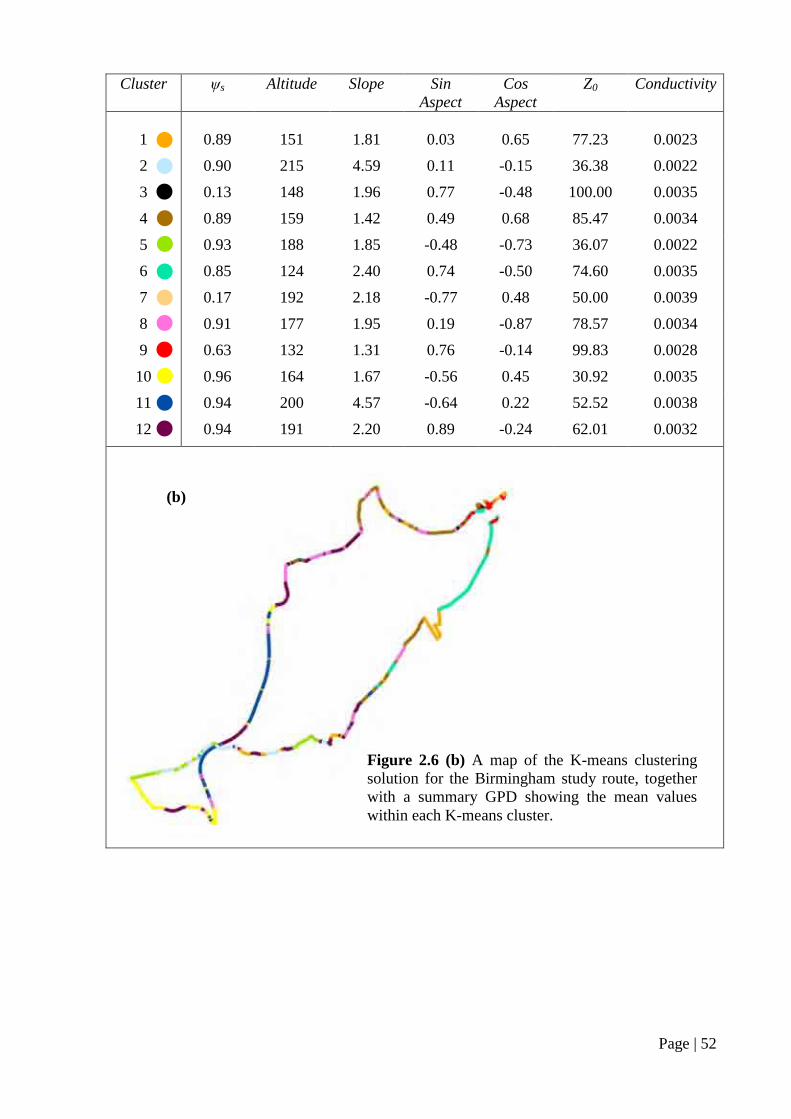
Page | 52
Cluster ψs Altitude Slope Sin
Aspect
Cos
Aspect
Z0
Conductivity
1 0.89 151 1.81 0.03 0.65 77.23 0.0023
2 0.90 215 4.59 0.11 -0.15 36.38 0.0022
3 0.13 148 1.96 0.77 -0.48 100.00 0.0035
4 0.89 159 1.42 0.49 0.68 85.47 0.0034
5 0.93 188 1.85 -0.48 -0.73 36.07 0.0022
6 0.85 124 2.40 0.74 -0.50 74.60 0.0035
7 0.17 192 2.18 -0.77 0.48 50.00 0.0039
8 0.91 177 1.95 0.19 -0.87 78.57 0.0034
9 0.63 132 1.31 0.76 -0.14 99.83 0.0028
10 0.96 164 1.67 -0.56 0.45 30.92 0.0035
11 0.94 200 4.57 -0.64 0.22 52.52 0.0038
12 0.94 191 2.20 0.89 -0.24 62.01 0.0032
(b)
Figure 2.6 (b) A map of the K-means clustering
solution for the Birmingham study route, together
with a summary GPD showing the mean values
within each K-means cluster.

Page | 53
The statistics in Table 2.4 (a) and (b) reveal how the performance of the forecast model can be
better assessed by analysing the statistics at a cluster level. The statistics presented in this
table are the standard forecast validation statistics used within the road weather industry for
assessing road weather model performance. These statistical terms, which are defined in the
mathematical description of ENTICE route-based forecast statistics at the start of the thesis,
include the model bias ( ), standard deviation of bias ( ), root mean square error (RMSE) of
the forecast, and the percentage of modelled (Pm) and residual modelled (Prm) forecast points
within ± 1°C of the actual and residual actual values. Where entire route statistics are given,
these are the average values based on all forecast points around the study route, and where
cluster level statistics are given, these are average values based on all forecast points within
that cluster. Unless otherwise stated, all the forecast validation statistics presented in this
thesis are an average of 20 thermal mapping runs of the study route.
The model statistics shown in Table 2.4 (a) and (b) were obtained with the ENTICE model
run in ‘quasi-operational’ mode, with all the parameters within the model set to their best
values. A low is an indicator of similar thermal characteristics between forecast points, so
a good clustering solution should aim to reduce the within as many clusters as possible to a
value below that for the entire route, hence making the clusters more distinct. Of the twelve
clusters shown in Table 2.4 (a) and (b), only three clusters in Table 2.4 (a) (clusters 1, 10 and
11) and two clusters in Table 2.4 (b) (clusters 7 and 10) have values greater than the
overall route statistic, indicating that thermal variations around the road network are well
represented by both clustering solutions. The significantly higher values in clusters 10 and
11 in Table 2.4 (a) and cluster 7 in Table 2.4 (b) can be explained by the fact that all of these
clusters contain forecast points located under bridges or underpasses, locations which the
model is known to be less accurate in forecasting for due to the lack of any advective
component in the zero-dimensional heat balance model. The marginally higher values in

Page | 54
cluster 1 in Table 2.4 (a) and cluster 10 in Table 2.4 (b) are likely to be the result of varying
ψs values within these clusters due to increased vegetation in rural locations where accuracy
of the proxy method of ψs data collection is known to be more variable (Chapman & Thornes
2006). The accuracy of statistics regarding actual temperatures can sometimes be misleading
since they are heavily dependent on the accuracy of the meteorological input data, so an
analysis of the percentage of correct residuals (Prm) is useful for assessing a model’s spatial
forecasting performance (Chapman et al. 2001b). The residuals in Table 2.4 (a) for the
hierarchical clustering solution reveal that in some clusters the model was 100% residually
correct to within ±1°C, and in 9 of the 12 clusters which together account for 89% of the
entire study route, the residual statistics are significantly better than the overall route statistic
would otherwise indicate. Similarly, Table 2.4 (b) reveals that the residual statistics in 9 of the
12 clusters for the K-means solution are also significantly better that the overall route statistic
would otherwise indicate, with these clusters accounting for 91% of the entire study route.

Page | 55
Table 2.4 (a) Route-based forecast validation statistics for the study route calculated for
individual hierarchical clusters. Entire route statistics represent the validation statistics
obtained using the existing methodology. (b) The same as (a), but for K-means clustering.
RMSE Pm Prm No. Forecast
Points
Entire Route -1.06 0.86 1.48 46.94 79.56 2261
(a)
Cluster 1 -0.77 0.87 1.32 46.97 78.45 216
Cluster 2 -0.29 0.55 0.83 77.30 94.38 200
Cluster 3 -0.78 0.00 0.99 55.00 100.00 1
Cluster 4 -2.32 0.73 2.45 9.53 85.00 128
Cluster 5 -1.12 0.70 1.45 44.80 87.01 1196
Cluster 6 -0.55 0.54 0.98 67.68 91.92 125
Cluster 7 -0.97 0.52 1.23 50.73 93.80 192
Cluster 8 -0.32 0.20 0.70 76.71 100.00 35
Cluster 9 -1.46 0.71 1.71 30.11 83.24 142
Cluster 10 -2.89 1.35 3.10 12.50 60.00 2
Cluster 11 -2.30 1.17 2.66 16.52 57.17 23
Cluster 12 -0.12 0.00 0.54 95.00 100.00 1
(b)
Cluster 1 -0.89 0.66 1.48 41.80 87.43 269
Cluster 2 -0.76 0.58 1.12 58.92 91.01 134
Cluster 3 -2.30 0.00 2.66 16.52 57.17 23
Cluster 4 -1.17 0.69 1.47 45.28 87.20 394
Cluster 5 -1.02 0.51 1.25 49.85 94.35 131
Cluster 6 -1.62 0.66 1.85 20.64 86.58 250
Cluster 7 -2.89 1.35 3.10 12.50 60.00 2
Cluster 8 -0.88 0.64 1.21 56.85 90.16 252
Cluster 9 -2.29 0.70 2.41 9.41 85.62 145
Cluster 10 -0.73 0.92 1.33 47.37 75.44 169
Cluster 11 -0.30 0.58 0.85 76.40 93.06 186
Cluster 12 -0.75 0.00 1.09 58.86 93.14 306

Page | 56
2.4 Consistency of the Clustering Techniques
To quantify the consistency of the clustering techniques, Clustering Similarity Coefficients
(CSC) were calculated for pairs of thermal mapping runs in the same weather category in
order to measure the similarity of the spatial distribution of RST variation identified by the
clustering solutions. CSC are calculated in a similar manner to Section Similarity Coefficients
used in thermal mapping (Shao et al. 1996), but use clusters determined by the geography and
road infrastructure around a route rather than sections determined by temperature variations
around a route. For two independent thermal mapping runs in the same weather category, the
mean temperature of a cluster is compared to the series mean and is assigned a positive sign if
the cluster mean is greater than or equal to the series mean, or a negative sign if the cluster
mean is less than the series mean. If the signs of the first clusters of both series are the same, a
= 1. If the signs of the next clusters in both series are the same, a = a+1, otherwise b = b+1 if
the signs are different. Once the values of a and b are calculated for each pair of series, CSC
are calculated as follows:
(2.5)
The higher the value of CSC between two series, the greater the similarity of spatial
temperature distribution between the series and the better the clustering solution is at
capturing the physical relation between measured RST and the geographical and road
infrastructure parameters used in the clustering solution. To assess the ability of both
clustering techniques at capturing this physical relation, a CSC analysis was performed on
pairs of thermal mapping runs for the study route. A total of 9 thermal mapping runs collected
under various weather conditions (3 damped, 3 intermediate and 3 extreme) were analysed
(Table 2.5). Results of the CSC analysis for both the hierarchical and K-means clustering
solutions are shown in Table 2.6. It is seen from the table that the CSC vary from 0.75 to 1.00

Page | 57
with a mean of 0.87 over all weather categories for the hierarchical clustered data set, and
from 0.67 to 1.00 with a mean of 0.91 for the K-means clustered data set. For individual
weather categories, mean values ranged from 0.83 (Damped & Intermediate) to 0.95
(Extreme) for the hierarchical clustered data set, and from 0.78 (Damped) to 1.00
(Intermediate) for the K-means data set. This means that the clustering solutions successfully
capture the physical relation between measured RST around the study route and the
geographical and road infrastructure parameters used to cluster the data sets, with the spatial
distribution of temperature around the study route repeatable for all three weather categories.
Table 2.5 Minimum, maximum, mean and of RST (°C) and category of thermal mapping
(TM) fingerprint.
TM run Date Min Max Mean Category
Damped (1) 13/01/00 -0.07 5.92 1.94 0.84 Damped
Damped (2) 29/02/00 2.68 7.01 4.21 0.57 Damped
Damped (3) 06/03/00 4.87 8.49 6.42 0.51 Damped
Intermediate (1) 10/12/99 3.04 9.36 5.16 1.00 Intermediate
Intermediate (2) 13/12/99 -0.95 7.14 1.69 1.12 Intermediate
Intermediate (3) 15/12/99 -2.47 4.32 -0.31 0.99 Intermediate
Extreme (1) 20/12/99 -7.01 3.63 -3.26 1.65 Extreme
Extreme (2) 14/02/00 -3.53 6.54 -0.29 1.42 Extreme
Extreme (3) 22/02/00 -4.01 4.81 -0.58 1.42 Extreme

Page | 58
Table 2.6 Clustering similarity coefficients (CSC) for independent pairs of thermal mapping
runs in the same weather category, calculated using hierarchical clustered forecast points (a)
and K-means clustered forecast points (b).
TM pairs No. of records No. of clusters CSC (a) CSC (b)
Damped (1,2) 2261 12 0.75 0.67
Damped (1,3) 2261 12 0.83 0.92
Damped (2,3) 2261 12 0.92 0.75
Intermediate (1,2) 2261 12 0.75 1.00
Intermediate (1,3) 2261 12 0.83 1.00
Intermediate (2,3) 2261 12 0.92 1.00
Extreme (1,2) 2261 12 0.92 0.92
Extreme (1,3) 2261 12 1.00 1.00
Extreme (2,3) 2261 12 0.92 0.92
2.5 Comparison of Hierarchical and K-means Clustering
To test the significance of any differences between the means of the hierarchical and K-means
clustered datasets, an Independent Samples Students t-test was performed on the clustered
GPD values in Figure 2.6 (a) and (b). Table 2.7 displays the results of the Independent
Samples t-test, with group 1 representing hierarchical clustering and group 2 K-means
clustering. The group statistics show that the two clustering techniques produced similar
means over the 12 cluster solution (t = 0.123, p = 0.902), with the hierarchical values varying
a little more around their mean than the K-means values. With a Levene significance value
greater than 0.10 it can be assumed that the two clustering solutions have equal variances, and
since the significance value of the t-test is greater than 0.05 it is safe to conclude (95%
confidence level) that the clustering solutions obtained using the two techniques are extremely
similar, and the differences which do exist are highly marginal and probably due to chance (P
= 90.2%).

Page | 59
Table 2.7 SPSS output statistics for an Independent samples t test comparing clustered GPD
values for the hierarchical and K-means clustering solutions.
2.6 Implementing a Cluster Based Validation Strategy
The clustering of forecast points and the subsequent validation of a route-based forecast at the
cluster level presents the opportunity for new sampling strategies that have the potential to
reduce the number of points needing to be validated in order to verify a route-based forecast
accurately. The current methodology requires every forecast point along a route to be
thermally mapped in order to obtain a single set of validation statistics for the entire route.
Validation using clustering techniques, however, has been shown here to provide a more
representative measure of a model’s spatial forecasting ability. By calculating clustering
similarity coefficients the clustering techniques tested have been shown to repeatedly capture
the spatial distribution of temperature around a salting route and hence the physical relation
between measured RST and the geographical and road infrastructure parameters controlling
the clustering. Since the majority of thermal variations around the route are identified within
the clustering, and since the variance within most clusters is significantly lower than the entire
route average, validation of the full spatial extent of a route-based forecast can potentially be
achieved with fewer forecast points. Using the current methodology of thermal mapping, a
route-based forecast dataset could potentially be reduced by randomly sampling a smaller
Group Statistics
84 35.285231 65.9492132 7.1956491
84 34.074735 61.6993518 6.7319512
Group
1.00
2.00
Test
N Mean Std. Deviation
Std. Error
Mean
Independent Samples Test
Equal variances assumed
.082 .775 .123 166 .902 1.2104964 9.8537573 -18.2443 20.66534Test
F Sig.
Levene's Test for
Equali ty of Variances
t df Sig. (2-tai led)
Mean
Difference
Std. Error
Difference Lower Upper
95% Confidence
Interval of the
Difference
t-test for Equali ty of Means

Page | 60
number of forecast points from within each cluster. It is likely, however, that such a
methodology would still require large sections of a route to be driven in order to reach the
required points, and whilst driving routes can be dynamically optimised (Handa et al. 2007) to
reduce some of the associated wastage this would entail, such a methodology does not allow
for validation at the full temporal resolution of the forecast.
A more robust sampling strategy could involve the installation of low cost remote infrared
RST sensors at numerous forecast points covering all the clusters within a route. This research
has shown that such a sampling strategy would capture the spatial distribution of temperature
around the route whilst providing continuous data throughout the day and night to enable
validation of the route-based forecast at the full temporal resolution. Whilst this scale of data
reduction could be viewed with scepticism, it must not be forgotten that over the last two
decades traditional road outstations have been strategically located based on a limited number
of climatic zones within a region. The clustering of forecast points around a route is in effect
combining the old paradigm with the new to create high resolution climatic zones where
geographical and road infrastructure parameters have a greater influence on variations in RST
than the meteorological parameters. Hence, it is perhaps more appropriate to refer to these
high resolution climate zones as ‘geo-clusters’. Reducing validation to only a small number of
points, however, potentially reduces the ability to identify and model small scale thermal
singularities around the road network such as shallow bridge decks and katabatic frost
hollows. On the other hand, recent research by the UK Met Office (Brown et al. 2008)
suggests that thermal features such as these could soon be identified using downscaling
techniques on high resolution numerical weather prediction (NWP) models. This would
enable a cluster style validation strategy using remote infrared RST sensors to be
implemented without fear of safety compromises, knowing that any areas identified as ‘cold
spots’ through downscaling techniques would be well monitored and accounted for in the
route-based forecast.

Page | 61
CHAPTER TWO SUMMARY
A new methodology for verifying route-based forecasts is described that uses clustering
techniques to create clusters of forecast points with similar geographical and infrastructure
characteristics. This facilitates the analysis of forecast statistics at the cluster level, which is
found to improve statistical assessment of model performance since validation can be
achieved at a much higher resolution than the current methodology allows. Furthermore,
validation of the full spatial extent of a route-based forecast can be achieved with fewer
forecast points since the majority of thermal variations around the road network are well
represented by the clustering solutions. A new sampling strategy using remote infrared RST
sensors is proposed that potentially enables validation at a vastly improved spatial and
temporal resolution.
It is envisaged that the proposed validation technique could be used as a rapid integrity test
for future measurement techniques designed to improve upon existing parameterisations
within route-based forecast models. This will be put to the test in chapter 5 of this thesis by
verifying the integrity of the new re-parameterised road construction and surface roughness
measurements that are proposed in the following two chapters. Currently, both road
construction and surface roughness are not measured at the spatial scale demanded by a
route-based forecast. The following two chapters attempt to address this issue, starting with
road construction.

Page | 62
3. SPATIAL RE-PARAMETERISATION OF THE
ENTICE MODEL: PART 1 - ROAD CONSTRUCTION
3.1 Road Construction Modelling in Route-Based Forecasts
Variations in the thermal properties of materials used in road construction are a contributing
factor to subtle variations in RST around a road network (Chapman et al. 2001b), with the
thermal damping depth of a road dependent upon the materials of which it is composed.
Thornes (1984) modelled the road heat flux beneath the surface based on a five zone flexible
pavement that simulated the road construction at a motorway study site. However, to add a
spatial component to the model, there was a need to develop similar profiles for other classes
of road found in the UK. Chapman et al (2001b) proposed a modified simulation for non-
motorway roads by making subtle changes to the materials and thermal properties of the
model profile to represent the different road types accounted for in the ENTICE model (Table
3.1).
Table 3.1 The materials and thermal properties of the ordinal road construction profiles used
in ENTICE. Note: thermal diffusivity of asphalt, concrete and soil is assumed to be 0.7x10-
2cm
2sec
-1, 1.2x10
-2cm
2sec
-1, and 0.1x10
-2cm
2sec
-1 respectively (Chapman et al. 2001b).
Depth (cm) Motorway (1) A-Road (2) B-Road (3) C-Road (4)
Materials
0 - 4.5 Asphalt Asphalt Asphalt Asphalt
4.5 – 9 Asphalt Asphalt Asphalt Concrete
9 – 18 Asphalt Asphalt Concrete Concrete
18 – 36 Concrete Concrete Concrete Concrete
36 – 72 Concrete 80% Concrete
20% Subgrade/soil
50% Concrete
50% Subgrade/soil
Subgrade/soil
Over 72 Subgrade/soil Subgrade/soil Subgrade/soil Subgrade/soil
Average thermal conductivity
3.9x10⁻³
cal cm-1
sec-1
˚C
3.5x10⁻³
cal cm-1
sec-1
˚C
2.9x10⁻³
cal cm-1
sec-1
˚C
2.1x10⁻³
cal cm-1
sec-1
˚C
ENTICE assumes a flexible pavement with a constant damping depth of 72 cm split into five
calculation zones. Variations in the construction of this 72 cm profile with respect to materials
and thermal properties are parameterised in the model according to the ordinal road type

Page | 63
classification in the ENTICE GPD. These parameterisations are based on the assumption that
a higher road classification (e.g. motorway) will have a profile with a greater proportion of
asphalt and concrete at the expense of a soil sub-base (Table 3.1). In a sensitivity analysis on
the ENTICE model, Chapman et al. (2001b) showed that variations in road construction were
a significant factor controlling RST. By holding all geographical and infrastructure
parameters within the model constant with the exception of road construction, Chapman et al.
(2001b) found that ENTICE model predictions could explain up to 68% of the variation in
RST around a study route (Figure 3.1). Furthermore, the impact of road construction on the
prediction of RST was found to be most dominant at higher levels of atmospheric stability
(Figure 3.1), during which road surfaces are more vulnerable to freezing in the winter months.
Figure 3.1 The influence of road construction on RST modelling at different levels of
atmospheric stability, using actual RST data from 20 thermal mapping runs for comparison of
model performance. The standard deviation of each thermal mapping run is used as a proxy to
stability (Chapman et al. 2001b).
In general, however, approximations of road construction for different classes of road are
difficult as no universal design procedure exists, and validation of profile parameterisations
would require multiple road core samples. Not only are the costs associated with obtaining
road cores for model validation too prohibitive, but the site specific nature of road coring
makes it unsuitable for use over large areas as would be needed for route-based model
Standard deviation of thermal mapping run (increasing stability)
Co
rrel
atio
n o
f m
od
elle
d R
ST
and
act
ual
RS
T p
er s
urv
ey

Page | 64
validation. The successful delivery of a route-based forecasting service relies on the accurate
measurement of road construction at every forecast point around a route. The ENTICE model
falls short in this respect since the parameterisation of road construction is based on an ordinal
classification of road type which lacks the sophistication exhibited by other components of
the model and fails to account for subtle variations in road construction around a route.
Bridge decks add further complexity to the issue, since the sudden change in construction
from a standard road surface to a bridge deck of shallower construction can often result in a
thermal singularity where the RST may be significantly lower. As a result, highway
authorities often commission high resolution thermal mapping surveys of such areas to inform
them of ice risk on bridges. The current methodology for parameterising road construction in
ENTICE, however, fails to take into account the significant impact of bridge decks on RST.
The original methodology used for locating bridges relies on manual identification from
1:50000 maps, and whilst there is some potential to use automated algorithms in GIS
packages for this task, these are not widely implemented. Specific construction data is rarely
available for all bridges, and hence, often the road type classification is simply lowered by a
category to account for the shallower construction encountered on bridge decks. Whilst such a
process may be a cost effective solution, it is clearly too simplistic since it fails to account for
any variations in bridge construction. Furthermore, it fails to account for smaller bridges that
may not appear on maps, are missed by human error, or conflict automatic GIS detection
techniques.

Page | 65
3.2 Ground Penetrating Radar
Ground Penetrating Radar (GPR) is a non-invasive geophysical technique that can be used to
detect electrical discontinuities in the shallow subsurface (< 50m) by generation,
transmission, propagation, reflection and reception of discrete pulses of electromagnetic
energy in the megahertz (MHz) frequency range (Neal 2004). The origins of GPR date back
to the early 20th
century when scientists were attempting to patent techniques to investigate
the nature of various buried features (Reynolds, 1997), and following these initial
developments GPR was primarily used in studies of glaciology (Plewes & Hubbard, 2001;
cited in Neal, 2004) until the 1970s when civil engineering, archaeological and geological
applications for GPR became more frequent (Reynolds, 1997; Conyers & Goodman, 1997).
The advent of digital data collection in the 1980s led to the first commercially available GPR
systems, and since the mid-1990s the technique has increasingly been used by the geology
and sedimentology research communities as a cost effective method of investigating the
shallow subsurface for purposes such as the reconstruction of past depositional environments
or for groundwater reservoir characterisation (Neal 2004).
Beyond the geological applications of GPR, the technology is widely used in a variety of
other fields including the highway industry where it is regularly used to assess the
performance and structure of roadways (Al-Qadi & Lahouar 2005). GPR technology was first
used on roads in the mid-1970s when tests were performed by the US FHWA on the
feasibility of using radars in tunnel applications (Morey 1998). In 1985 the first vehicle
mounted GPR system for highways was developed under a FHWA contract, and this led to a
rapid expansion in the use of GPR technology for evaluating subsurface conditions for
transportation facilities. From the mid-1990s onwards GPR has primarily been used for road
layer thickness estimation and the identification of moisture accumulation within road layers.
Accurate predictions of road layer thicknesses provide important data for roadway
management systems since they are needed for overlay design, quality control and for

Page | 66
structural capacity estimation of existing roads to predict their remaining serviceable life (Al-
Qadi & Lahouar 2005).
3.2.1 Calculating layer depth
In road applications, the GPR technique is based on the principle of sending a short
electromagnetic pulse through an antenna to the road surface and then recording the reflected
pulses from the surface and any subsurface layer interfaces bearing discontinuities in
electrical properties. The time difference measured between the reflected pulses, known as the
two-way travel time, can be used together with the dielectric properties of the surveyed layer
to determine layer thickness using Equation 3.1 (Wimsatt et al. 1998):
√ (3.1)
where di is the thickness of the ith layer, ti is the electromagnetic pulse two-way travel time
through the ith layer, c is the speed of light in free space (c = 3 x 10⁸ m/s) and εr,i is the
dielectric constant of the ith layer.
The main difficulty in interpreting GPR data for measuring the thickness of road layers is
illustrated by Equation 3.1. Specifically, if it is assumed that the two-way travel time ti can be
accurately measured from the GPR signal, the dielectric constant of the material within the
layer being measured remains unknown. Road layers are typically composed of various
construction materials such as asphalt binder, aggregate, air-voids and water, all of which
combine to make physically inhomogeneous layers. Since the bulk dielectric properties of an
inhomogeneous material are typically a combination of the dielectric properties and volume
proportions of the individual components, the dielectric properties of road layers will vary
both between layers and within layers depending on the mixtures used. Furthermore, the
dielectric properties of road layers are greatly affected by rain and the resulting moisture
accumulation within road layers, and consequently their values are usually unknown and are

Page | 67
difficult to predict. This problem has resulted in a wealth of research over the past decade
focused towards the development of data analysis algorithms for better estimation of the
dielectric constant of different road layers (Al-Qadi & Lahouar 2005; Lahouar & Al-Qadi
2008). Such algorithms however are only necessary in applications requiring high levels of
accuracy, such as structural capacity estimation, and are beyond the scope of a pilot study
such as this.
3.2.2 GPR traces and radargrams
Data collected during a GPR survey is typically displayed as a trace (Figure 3.2), showing the
travel time of the electromagnetic pulse at a set location. Each inflexion in the trace represents
a discontinuity where there is potentially a change in the subsurface construction and hence a
change in thermal properties. Over the course of a survey, traces are obtained at a fixed spatial
resolution allowing a radargram to gradually be built up (Figure 3.3). These show cross-
sectional views of the subsurface, where the magnitude of reflected pulses from the surface
and any subsurface layer interfaces are plotted against their two-way travel time to reveal a
cross-sectional view of discontinuities / layers in the subsurface.
Figure 3.2 A sample GPR trace, showing the varying amplitude of the electromagnetic pulse
as it penetrates the subsurface.

Page | 68
Figure 3.3 (a) Radargram collected on a motorway showing a deep and uniform road
construction and (b) radargram collected on a minor c-road showing a less uniform, shallower
construction.
3.3 Application of GPR Data within the ENTICE Model
3.3.1 Data collection
To investigate the potential use of GPR data for modelling road construction in the ENTICE
route-based forecast model, a GPR survey of the Birmingham study route (Figure 2.3) was
undertaken using a Malå RoadCart GPR unit (Figure 3.4). The equipment setup included a
shielded 500 MHz low frequency antenna, designed for high speed GPR measurements on
roads, attached to a custom made trailer which also housed a differential GPS receiver capable
of sub-metre accuracy. Data from the GPR antenna was fed into a Malå CUII GPR control
unit with high frequency module and stored on a data logger. The RoadCart trailer was
attached by towbar to a Land Rover Freelander vehicle which was used to drive the study
route, and during the survey the GPR data could be viewed as a real-time radargram (Figure
3.3) on a Malå XV11 monitor positioned in the vehicle.
Surface reflection
Surface reflection
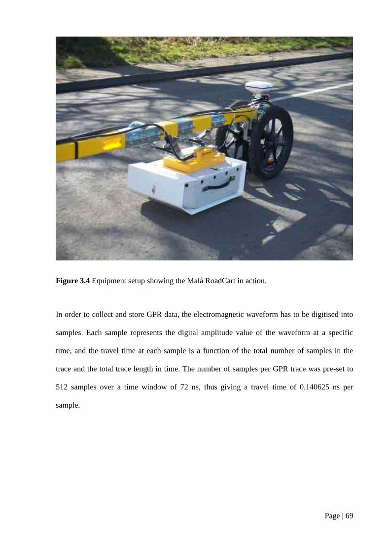
Page | 69
Figure 3.4 Equipment setup showing the Malå RoadCart in action.
In order to collect and store GPR data, the electromagnetic waveform has to be digitised into
samples. Each sample represents the digital amplitude value of the waveform at a specific
time, and the travel time at each sample is a function of the total number of samples in the
trace and the total trace length in time. The number of samples per GPR trace was pre-set to
512 samples over a time window of 72 ns, thus giving a travel time of 0.140625 ns per
sample.

Page | 70
3.3.2 Identification of bridge decks from radargrams
As a bridge deck represents (in most cases) a dramatic change in construction, the first goal
was to investigate if GPR had the capability to detect the three known bridge decks on the
study route. The radargrams associated with these bridges are shown in Figure 3.5. Figure 3.5
(a) shows a relatively small bridge deck located on the M5 motorway. Thermal mapping data
has previously shown that this bridge typically produces a thermal singularity under stable
conditions of about -0.3°C when compared to the adjoining carriageway. Changes in the
reflected GPR signal are clearly visible over the bridge section (Figure 3.5 (a)). The signal
received is a consequence of the air void under bridges which causes multiple direct air waves
to be returned rather than the normal reflections from subsurface discontinuities. Similar GPR
signals can be identified in Figure 3.5 (b) and (c) which show larger bridges crossing the M5
motorway. Of particular interest in Figure 3.5 (c) is the clear visibility of the pillars (P1 – P4)
at both sides of (and in-between) the two carriageways of the motorway. Instead of having a
lower RST common to most bridges, thermal mapping data has shown that the thermal
singularity on this bridge is typically +0.3°C warmer than the adjoining road sections under
stable atmospheric conditions. This can easily be explained, however, by the presence of
frequent standing traffic on the bridge caused by traffic lights at the motorway exit (Figure
3.6).
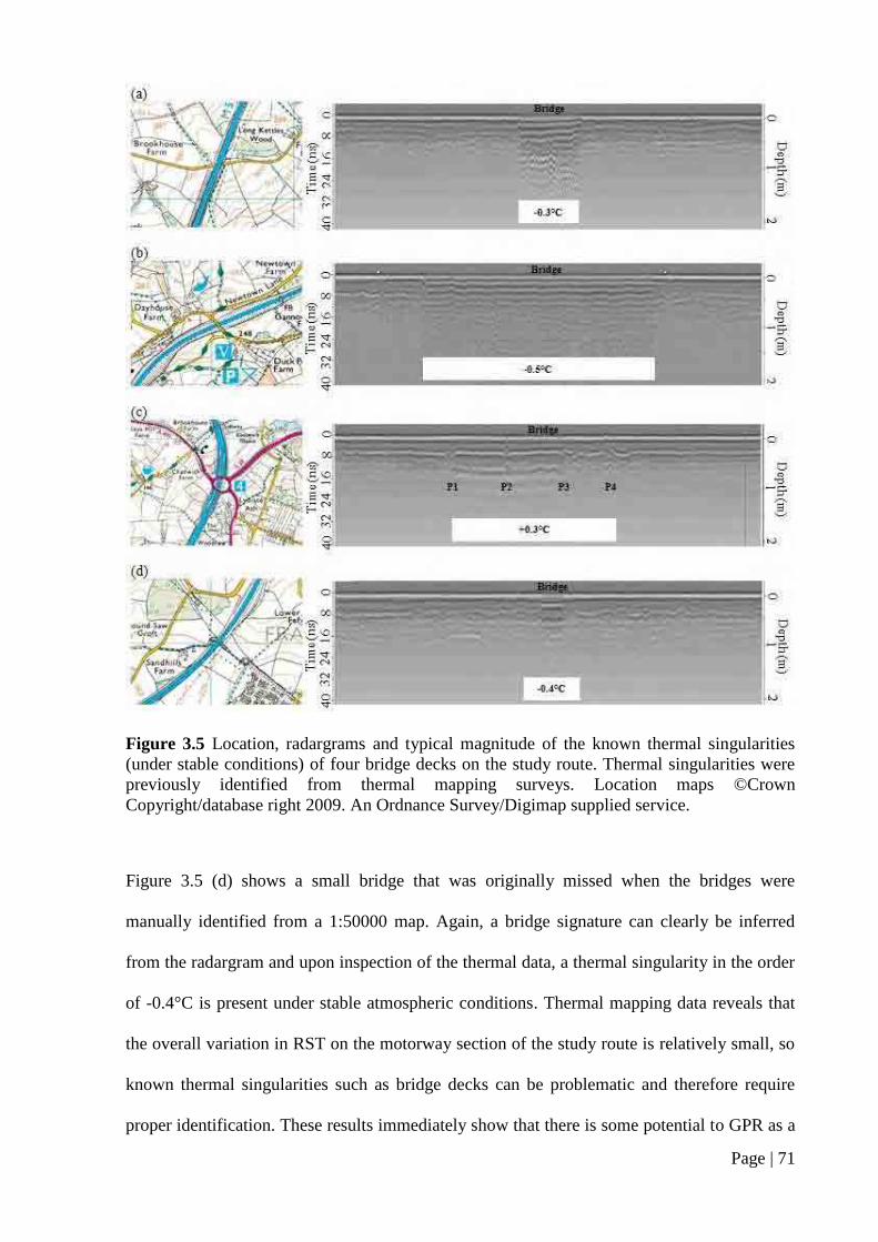
Page | 71
Figure 3.5 Location, radargrams and typical magnitude of the known thermal singularities
(under stable conditions) of four bridge decks on the study route. Thermal singularities were
previously identified from thermal mapping surveys. Location maps ©Crown
Copyright/database right 2009. An Ordnance Survey/Digimap supplied service.
Figure 3.5 (d) shows a small bridge that was originally missed when the bridges were
manually identified from a 1:50000 map. Again, a bridge signature can clearly be inferred
from the radargram and upon inspection of the thermal data, a thermal singularity in the order
of -0.4°C is present under stable atmospheric conditions. Thermal mapping data reveals that
the overall variation in RST on the motorway section of the study route is relatively small, so
known thermal singularities such as bridge decks can be problematic and therefore require
proper identification. These results immediately show that there is some potential to GPR as a

Page | 72
tool for locating even the smallest of bridges along routes from the analysis of radargrams. It
is clear that with minimal processing, bridge decks can be identified in a more objective
manner than manual identification from a map.
Figure 3.6 Aerial photograph of the motorway bridge identified in Figure 3.5(c), showing the
location of traffic lights on the bridge which often leads to standing traffic causing the warm
thermal singularity of +0.3°C observed at this location.
Traffic Lights

Page | 73
3.3.3 Subsurface layer depths
Based on the original ordinal road type classification and the associated road profiles (Table
3.1) initiated by Chapman et al. (2001b), we would expect to see variations in road
construction profiles around the study route as the road type varies. The two radargrams
shown in Figure 3.3 were collected from a motorway (Figure 3.3 (a)) and a minor C-road
(Figure 3.3 (b)) along the study route, and reveal differences in the road construction profile
between the two road types. The main differences are in the uniformity of the profiles, with
the motorway section appearing to have a deeper and more uniform construction than the
minor C-road. However, despite the more uniform nature of the motorway profile, subtle
fluctuations in the subsurface horizons are still evident, and the ordinal road profiles currently
used in the ENTICE model (Table 3.1) are too simplistic to enable such fluctuations to be
quantified and accounted for in the parameterisation of subsurface temperatures.
In an attempt to re-parameterise the road construction profile in the ENTICE model for each
forecast point along the study route, an inflexion point detection algorithm (Appendix 2)
capable of analysing the digitised electromagnetic waveform of each GPR trace for evidence
of subsurface horizons/discontinuities was developed. Firstly, an Exponentially Weighted
Moving Average (EWMA) was applied to the raw GPR data over an average of 5 GPR traces,
corresponding to 5 metres of road length. Applying an EWMA to a dataset helps to reduce
noise in the dataset whilst keeping the lag associated with moving averages to a minimum.
Typical noise for GPR data from roads could include erroneous measurements from objects
such as drainage covers or underground utility pipes which distort the GPR signal. Next, the
EWMA modified GPR dataset was spatially joined to the ENTICE GPD for the study route
using the spatial join feature available in ESRI ArcMap. The modified GPD, which now
included the digitised electromagnetic waveform of the GPR trace for each forecast point, was
then loaded into Matlab ready to be analysed by the inflexion point detection algorithm
(Appendix 2).

Page | 74
The inflexion algorithm maintains the existing ENTICE parameterisation of a five zone
flexible pavement whose layer materials vary according to road type (Table 3.1). Hence, the
algorithm attempts to identify 5 subsurface layer interfaces/discontinuities by searching for
significant inflexions in the electromagnetic waveforms forming the GPR traces measured at
each point along the study route. Once an inflexion is identified, the travel time associated
with this inflexion is calculated and assigned to this point in the GPR trace, and the algorithm
then continues to search for further inflexions within the same GPR trace. Once no more
inflexions can be found within a trace, the algorithm moves onto the next trace (next point
along the route) and the same process is repeated until the GPR trace at every point along the
study route has been examined for subsurface layer interfaces.
The algorithm then calculates the depths of all identified layers in each trace using Equation
3.1, assigning dielectric constant values to each layer based on the materials assigned to each
layer in the existing ENTICE road type parameterisation (Table 3.1). Hence, for a point
located on a motorway, the top three layers in the road profile are assigned a dielectric value
of 6 in Equation 3.1 to represent asphalt, whilst the bottom two layers are assigned a dielectric
value of 10 corresponding to concrete. In contrast, where points are located on a minor C-road
only the top layer is assigned a dielectric value of 6 (asphalt), with the middle three layers
assigned a dielectric value of 10 (concrete) and the bottom layer a value of 25 to represent a
soil layer. The dielectric constants used are approximate values taken from the Malå
GroundVision software manual and represent typical values for these materials based on an
unsaturated media. In reality, for the reasons highlighted in section 3.2.1 the differences in the
dielectric values between layers will vary considerably along the study route, but without road
core data to verify the subsurface materials at each point, such approximations are necessary
for modelling purposes.

Page | 75
0 500 1000 1500 2000
-1.2
-1
-0.8
-0.6
-0.4
-0.2
0
Forecast points along study route
De
pth
be
low
su
rfa
ce
(m
etr
es)
Interface 1
Interface 2
Interface 3
Interface 4
Interface 5
Figure 3.7 Calculated depths of subsurface interfaces at each forecast point along the study
route, assuming a five zone flexible pavement with material composition matching that of the
existing ENTICE road construction parameterisation shown in Table 3.1.
Initial analysis of the calculated depths from the inflexion algorithm revealed difficulties in
identifying the lower two subsurface interfaces over the majority of the study route, most
likely due to poorer than expected penetration depth with the 500 MHz antenna. Whilst it was
expected that a 500 MHz antenna would provide a good balance between resolution and
signal penetration depth, in hindsight a lower frequency antenna, perhaps 250 MHz, would
have given a better balance and provided greater depth penetration. To overcome this problem
and enable the modelling of a five zone flexible pavement to continue, the depths (thickness)
of the fourth and fifth layer interfaces were pre-set to the existing ENTICE values of 18 cm
and 36 cm respectively, with the total depth of these layers from the surface dependent on the
thickness of the upper three layers which varied based on the GPR measurements. Figure 3.7
reveals the depths of the five subsurface interfaces at each forecast point calculated by the

Page | 76
inflexion algorithm, and Table 3.2 summarises the average depths of each layer and the total
average profile depth for each of the road type classifications in the ENTICE model.
Table 3.2 Average depths for each layer of the re-parameterised five zone flexible pavement
in the ENTICE model, based on analysis of the digitised electromagnetic waveform data from
a GPR survey using an algorithm (Appendix 2) designed to identify subsurface interfaces
from significant inflexions in the waveform of individual GPR traces.
Motorway (1) A-Road (2) B-Road (3) C-Road (4)
Layer 1
Av. Depth (cm)
Asphalt
6.5
Asphalt
6.8
Asphalt
6.8
Asphalt
7.1
Layer 2
Av. Depth (cm)
Asphalt
8.8
Asphalt
7.9
Asphalt
7.7
Concrete
5.1
Layer 3
Av. Depth (cm)
Asphalt
14.4
Asphalt
14.2
Concrete
14.1
Concrete
9.1
Layer 4
Av. Depth (cm)
Concrete
18
Concrete
18
Concrete
18
Concrete
18
Layer 5
Av. Depth (cm)
Concrete
36
80% Concrete
20% Subgrade/soil
36
50% Concrete
50% Subgrade/soil
36
Subgrade/soil
36
Total Depth (cm)
83.7
83
82.5
75.3
Average thermal conductivity
4.09x10⁻³
cal
cm-1
sec-1
˚C
3.86x10⁻³
cal cm-1
sec-1
˚C
4.07x10⁻³
cal cm-1
sec-1
˚C
3.59x10⁻³
cal cm-1
sec-1
˚C
In the original ENTICE road type parameterisation (Table 3.1) the depth of each layer in the
five zone flexible pavement is assumed to be constant with no variation between road type.
The new parameterisation (Table 3.2) derived from GPR measurements attempts to improve
upon this by identifying real changes in the depth of the upper three layers of the five zone
profile at each forecast point. With the incorporation of GPR measurements, the total average
depth of the five zone profile varies between the different road types in the ENTICE model,
with motorways on average having a slightly deeper construction than A and B roads, and C-
roads displaying the shallowest construction as we would expect for minor lower trafficked
roads (Table 3.2). The GPR measurements reveal that the average depth of the uppermost
asphalt layer is greatest on the minor C-roads (7.1 cm) and most shallow on the motorway
sections of the study route (6.5 cm), possibly the result of greater wear on the motorway

Page | 77
surface due to the higher volume of traffic on these roads. However, the increased strength
and stability of the motorway roads compared to the minor C-roads is evident in the second
and third subsurface layers, whose combined average depth is some 9 cm greater at motorway
locations due to the more stringent design procedures for motorways that are designed to
withstand much higher traffic loads.
Average thermal conductivity values calculated for the four road profiles in Table 3.2 are
derived from thermal conductivity values for asphalt, concrete and soil that have been altered
from the original ENTICE values due to numerous inconsistencies in the literature. In the
original Thornes (1984) model, thermal conductivity values of 0.0048 and 0.0031 cal cm-1
sec-1 °C were used for concrete and asphalt respectively, and the thermal conductivity of soil
was assumed to be the same as that of concrete. Chapman et al. (2001b) used these values to
calculate an average thermal conductivity for each road type in the ENTICE model based on
the materials and depths of each zone of the five zone flexible pavement (Table 3.1).
However, the thermal conductivity of asphalt and concrete varies considerably depending
upon the exact composition of the materials used to produce the end product, and likewise the
ability of different soils to conduct heat will vary based on factors such as the density and
chemical composition of the soil. To bring an element of consistency to road weather models,
it was decided that ENTICE would use the same thermal conductivity values that are
implemented in the METRo model, which is probably the most widely used heat balance
model in road weather forecasting as a result of the MDSS project in the US (Chapter 1).
Hence, thermal conductivity values for concrete, asphalt and soil in the ENTICE model were
altered to 0.0053, 0.0019 and 0.0024 cal cm-1
sec-1 °C respectively (Crevier & Delage 2001),
giving average values for the original ENTICE 72 cm pavement parameterisation of 0.00438,
0.00410, 0.00409 and 0.00359 cal cm-1
sec-1 °C for motorways, A-roads, B-roads and minor
C-roads respectively:

Page | 78
for all forecast points do
set depth of road construction to 72 cm
if road type = 3000 (motorway)
set thermal conductivity to 0.00438 cal cm-1
sec-1 °C
else if road type = 3001 (A-road)
set thermal conductivity to 0.00410 cal cm-1
sec-1 °C
else if road type = 3002 (B-road)
set thermal conductivity to 0.00409 cal cm-1
sec-1 °C
else if road type = 3004 (C-road)
set thermal conductivity to 0.00359 cal cm-1
sec-1 °C
else
set thermal conductivity to default value (motorway)
end if
end for
To assess the impact of these altered thermal conductivity values on the spatial forecasting
performance of ENTICE, statistical analysis was conducted on 20 nights thermal mapping
data for the study route. During these tests all of the geographical parameters in the model,
with the exception of road type, were fixed spatially to default values, rather than running the
model in ‘quasi-operational’ mode. By fixing all other geographical parameters spatially, it
ensures any changes identified in the model forecast are solely due to the change in thermal
conductivity. If the model were run in ‘quasi-operational’ mode in this instance, then changes
to road type in the model would also lead to changes in Z0 since Z0 varies in the model with
respect to the ordinal land use and road type classification (Chapter 4), making it impossible
to quantify the effect of road type changes alone on model performance. By fixing all other
geographical parameters spatially, the resultant forecast statistics are not providing a true
measure of model performance, but instead are a reflection of model bias caused by the
spatial fixing of the geographical parameters. However, by running the model twice, first
using the original thermal conductivity (road type) values (Table 3.1) and again using the
newly calculated averages based on the thermal conductivity values used in the METRo
model, changes in the model results between the two model runs enables us to quantify the

Page | 79
impact of thermal conductivity changes on model performance. Forecast statistics for both
model runs are summarised in Table 3.3.

Page | 80
Table 3.3 Forecast statistics from a statistical analysis on average thermal conductivity profiles in ENTICE, where all geographical variables in the
model were held constant with the exception of road type.
Analysis 1 – Using original ENTICE thermal conductivity
values
Analysis 2 – Using METRo based thermal conductivity
values
Night RMSE Pm Prm R2 RMSE Pm Prm R
2
1 -0.58 0.96 1.12 69.79 72.98 0.23 -0.48 0.98 1.09 70.32 72.00 0.24
2 0.09 1.10 1.10 67.76 69.48 0.08 0.22 1.11 1.13 64.35 69.70 0.08
3 -1.44 1.30 1.94 40.78 59.71 0.14 -1.26 1.32 1.83 43.61 58.43 0.14
4 -0.6 0.96 1.13 67.01 71.61 0.18 -0.52 0.97 1.10 67.45 70.15 0.19
5 -1.45 1.43 2.04 48.70 55.11 0.10 -1.21 1.46 1.89 54.18 55.51 0.10
6 -1.13 1.44 1.83 55.86 52.28 0.05 -0.89 1.45 1.70 60.11 52.19 0.05
7 -1.51 1.57 2.18 36.22 52.10 0.13 -1.24 1.60 2.02 41.13 51.53 0.13
8 -0.10 0.77 0.77 83.37 82.57 0.19 0.16 0.79 0.81 78.77 80.19 0.19
9 -2.19 0.90 2.37 6.10 77.00 0.11 -1.98 0.92 2.19 12.43 74.88 0.07
10 -0.71 1.11 1.31 66.74 74.13 0.06 -0.28 1.10 1.14 72.89 71.07 0.07
11 -0.76 0.77 1.08 67.58 84.52 0.13 -0.65 0.78 1.01 71.21 83.19 0.14
12 0.54 1.38 1.48 46.57 65.72 0.06 0.98 1.38 1.69 32.77 64.31 0.08
13 -0.22 0.89 0.92 79.39 81.16 0.08 0.08 0.90 0.90 76.82 78.55 0.10
14 0.28 0.71 0.76 79.30 87.93 0.19 0.34 0.72 0.79 75.54 86.73 0.20
15 0.15 1.33 1.34 58.43 61.88 0.12 0.70 1.34 1.51 43.92 61.34 0.14
16 -0.01 0.56 0.56 93.68 93.72 0.05 0.04 0.57 0.57 93.41 93.59 0.05
17 -0.50 1.16 1.26 67.71 66.34 0.10 -0.13 1.16 1.17 65.68 65.28 0.12
18 -1.40 0.96 1.70 37.51 78.24 0.17 -0.94 0.97 1.35 59.22 75.90 0.18
19 -1.08 0.48 1.18 50.60 95.40 0.15 -0.83 0.47 0.95 70.28 96.28 0.16
20 -1.62 0.90 1.85 25.48 78.51 0.10 -1.30 0.90 1.59 36.36 77.27 0.11
Average -0.71 1.03 1.40 57.43 73.02 0.12 -0.46 1.04 1.32 59.52 71.90 0.13

Page | 81
The statistics in Table 3.3 reveal an improvement in the RMSE of the route-based forecast,
indicating that the magnitude of any errors in the forecasts has been reduced by using the new
thermal conductivity values, which is reflected by a reduction in the negative bias of the
forecast of 0.25°C, with only a marginal increase in . The overall percentage of modelled
forecast values within ±1°C of the actual values (Pm) has increased by 2.09%, whilst the
percentage of residual modelled forecast values within ±1°C of the residual actual values
(Prm) decreases by a smaller margin (1.12%). Whilst such statistics are a good indicator of
the spatial forecasting ability of a model, they are nonetheless limited to a resolution of ±1°C,
and can potentially ignore finer scale improvements to a model. Analysis of the coefficient of
determination (R2) for modelled versus actual RST is a further method of analysing the spatial
forecasting performance of ENTICE which, unlike the Pm and Prm values, is not limited by
temperature resolution. Analysis of the R2 values for modelled versus actual RST reveals a
small increase (1%) in the variability of RST accounted for by ENTICE with the new thermal
conductivity values. Hence, using the new average thermal conductivity profiles with the
original ENTICE five zone fixed depth pavement parameterisation, a small improvement is
observed in the overall spatial forecasting performance of the ENTICE model when run in a
non ‘quasi-operational’ mode.
Despite the observed improvement in forecasting performance with the new thermal
conductivity profiles, these are still based on the existing road type parameterisation in
ENTICE (Table 3.1) which is clearly too simplistic since it fails to account for the clear
differences in subsurface layer depths between road types identified in the GPR
measurements. Such variations in road profiles are important and should be included in the
forecast model since they have a direct effect on the surface heat flux controlling the thermal
memory of the road surface.

Page | 82
3.3.4 Surface heat flux
Thermal memory is a term used to describe the length of time which a surface stores heat
from daytime solar radiation (Thornes 1991). The thermal damping depth in a road obviously
depends upon the materials of which it is composed, and the changes in construction depth
along the study route identified from the GPR survey (Figure 3.7 & Table 3.2) will have an
impact on the thermal damping depth around the study route. Outcalt (1972) assumed that the
temperature at the damping depth of the ground equalled the temperature at the damping
depth in the atmosphere, with no attempts made to measure temperatures at depth in the
ground. Thornes (1984) used temperature measurements at 36 cm and 18 cm below the
surface, with the temperature at 36 cm taken to be the temperature half way between the
surface and a damping depth of 72 cm. A damping depth of 72 cm was seen by Thornes
(1984) as being reasonable since it lies between the damping depths for asphalt and concrete.
Thermal memory is accounted for in ENTICE through calculation of the surface heat flux at
each forecast point. Assuming a constant damping depth of 72 cm, ENTICE calculates the soil
temperature change at each layer of the five zone flexible pavement, starting with the soil
temperature change midway between the surface and the damping depth, i.e. 36 cm, and then
halving the distance to the surface at each computation level. The soil heat flux is then
calculated between the surface and a depth one-sixteenth the depth of thermal damping
(Outcalt 1972), which currently equates to a constant depth of 4.5 cm at every forecast point
in the model. The heat flow in ENTICE is described by a one-dimensional conduction
equation described by Thornes (1984) such that at depth ZU:
( ( )
) (3.2)
where RD is the thermal diffusivity and TX the temperature at depth (2 x ZU). The heat flux is
calculated as follows:

Page | 83
( )( ) (3.3)
where RK is the thermal conductivity, ZU is the depth 4.5 cm, and TU is the temperature at
depth ZU.
To incorporate the changes in layer depth identified through the GPR measurements (Figure
3.7), the ENTICE model code was modified to include the newly calculated depths for the
upper three subsurface layers within the calculation of average thermal conductivity profiles
at each forecast point. Firstly, the total depth ($ZG[$M]) at each forecast point was calculated
by summing the thicknesses of the upper three layers calculated via the GPR inflexion point
algorithm (Appendix 2), and adding these to the depth of the bottom two layers which was
pre-set to the existing ENTICE value of 54 cm as described in section 3.3.3. Next, an average
thermal conductivity value ($RKA[$M]) was calculated at each forecast point by calculating
the total depth of asphalt, concrete and soil within the profile and multiplying each of these by
their respective thermal conductivity values, and then summing these values and diving by the
total depth of the profile. The material assigned to each of the five layers was dependent on
the road type classification at each forecast point (Table 3.2).
for all forecast points do
calculate the total depth of road construction by adding the depths of the top three layers
together (calculated from GPR data), and adding an additional 54cm (to account for pre-set
depth of bottom two layers)
if road type = 3000 (motorway)
calculate average thermal conductivity by multiplying the depth of each subsurface
material (asphalt, concrete & soil) by the conductivity value for that material, then
summing these values and dividing by the total depth of road construction
repeat for all road types
end if
end for

Page | 84
In the ENTICE model, the total depth ($ZG[$M]) at each forecast point was used as the new
damping depth for each subsurface profile, and the soil temperature change was then
calculated at each layer starting with the temperature change at the interface of the fourth and
fifth subsurface layers ($ZT), followed by each of the other subsurface layer interfaces in turn
($ZZ, $ZX and $ZU) (see Appendix 5). As with the original ENTICE model, the soil heat
flux ($S[$I]) is then calculated between the surface and the first subsurface layer interface
($ZU), but unlike the original model the depth of this layer interface now varies at each
forecast point based on the calculated depths from the GPR measurements, rather than
remaining a constant 4.5 cm along the entire route.
3.4 Statistical Analysis of New Subsurface Parameterisation
To test whether the re-parameterised subsurface profiles at each forecast point improve the
spatial forecasting performance of ENTICE, further statistical analyses were conducted on the
same 20 nights thermal mapping data used throughout this study. Again, during this analysis
the geographical parameters in the model, with the exception of road type and traffic, were
fixed spatially to default values, instead of running the model in ‘quasi-operational’ mode, to
enable just the impact of thermal conductivity changes to be quantified. Traffic is also
included in the analysis to give an indication of the influence that the general traffic algorithm
used in ENTICE (Chapter 6) has on model performance. Again, the analysis was run twice,
first using the original ENTICE road construction parameterisation containing fixed layer
depths (Table 3.1), and again using the re-coded model which included the new average
thermal conductivity values and variable layer depths at each forecast point calculated from
the GPR measurements. The inclusion of traffic is acceptable since its impact remains the
same over both analyses, thus enabling us to quantify the impact of thermal conductivity

Page | 85
changes alone on model performance. Forecast statistics for both analyses are summarised in
Table 3.4.

Page | 86
Table 3.4 Forecast statistics from a statistical analysis on road construction parameterisation in the ENTICE model. Statistics in Analysis 1 relate to
modelled vs. actual RST using the original ENTICE road construction parameterisation proposed by Chapman et al. (2001b), and statistics in Analysis
2 relate to modelled vs. actual RST using the new re-parameterised subsurface road construction measurements derived from GPR data.
Analysis 1 – Using METRo based thermal conductivity
values, with traffic on
Analysis 2 – Using new thermal conductivity values
calculated from new depth profiles
Night RMSE Pm Prm R2 RMSE Pm Prm R
2
1 -1.60 0.86 1.82 22.60 84.03 0.26 -1.48 0.87 1.72 31.93 83.72 0.26
2 -0.88 1.06 1.38 63.78 71.83 0.14 -0.78 1.05 1.31 66.74 71.65 0.14
3 -2.38 1.19 2.66 5.44 68.20 0.23 -2.20 1.19 2.50 9.20 68.24 0.23
4 -1.59 0.89 1.82 25.65 75.94 0.22 -1.46 0.89 1.71 34.14 76.07 0.22
5 -2.38 1.43 2.78 13.45 58.65 0.10 -2.18 1.44 2.61 16.14 57.94 0.09
6 -2.08 1.49 2.55 19.55 58.03 0.06 -1.83 1.50 2.37 25.21 57.81 0.05
7 -2.38 1.49 2.80 13.93 49.49 0.18 -2.09 1.49 2.57 26.05 48.92 0.18
8 -1.12 0.79 1.37 46.70 82.18 0.26 -0.90 0.77 1.19 58.91 83.10 0.25
9 -3.12 0.95 3.26 0.93 74.35 0.16 -2.68 0.99 2.85 5.04 74.04 0.17
10 -1.60 1.21 2.01 30.87 65.72 0.10 -1.21 1.20 1.70 42.72 65.33 0.09
11 -1.74 0.76 1.90 14.55 83.28 0.21 -1.64 0.75 1.80 17.43 84.17 0.21
12 -0.27 1.37 1.39 70.10 65.02 0.15 0.29 1.39 1.42 54.22 62.80 0.14
13 -1.15 1.01 1.53 44.54 72.40 0.12 -0.82 1.01 1.30 58.03 72.93 0.10
14 -0.78 0.69 1.04 65.33 84.87 0.20 -0.63 0.71 0.94 70.28 84.12 0.21
15 -0.63 1.33 1.47 62.72 60.50 0.20 0.02 1.33 1.33 60.68 61.48 0.21
16 -1.07 0.71 1.28 38.92 84.56 0.05 -0.87 0.77 1.16 50.60 81.20 0.05
17 -1.39 1.17 1.82 41.00 66.92 0.16 -0.93 1.19 1.51 55.29 66.96 0.16
18 -2.29 1.00 2.50 4.95 75.06 0.26 -1.66 1.02 1.95 24.81 75.45 0.25
19 -2.07 0.74 2.20 11.37 80.76 0.14 -1.50 0.84 1.72 21.49 77.62 0.15
20 -2.51 0.97 2.69 6.02 74.35 0.15 -2.16 0.99 2.37 11.59 74.35 0.15
Average -1.65 1.06 2.01 30.12 71.81 0.17 -1.34 1.07 1.80 37.03 71.40 0.17

Page | 87
Comparing the statistics in Table 3.4 with those in Table 3.3 which do not take into account
the ENTICE traffic algorithm, it can be seen that the inclusion of traffic has increased the
negative bias of the forecast and the magnitude of any errors (Table 3.4), but the overall
variability of RST which is accounted for by the model has increased by 5% as shown by the
overall increase in the R2 value. From Table 3.4 it is clear that the magnitude of any errors in
the forecast is significantly reduced when the original fixed-depth subsurface parameterisation
is replaced by the new variable subsurface road profiles calculated from GPR measurements,
with the negative bias of the route-based forecast falling by 0.31°C and the RMSE by 0.21°C.
Another indicator of improved forecasting ability with the new variable subsurface
measurements is an increase of almost 7% in the overall Pm values (Table 3.4 & Figure 3.8),
with negligible change (-0.41%) in the Prm values. Analysis of the coefficient of
determination for modelled versus actual RST (Table 3.4 & Figure 3.9) reveals little change
in the overall variability of RST which is accounted for by the model.
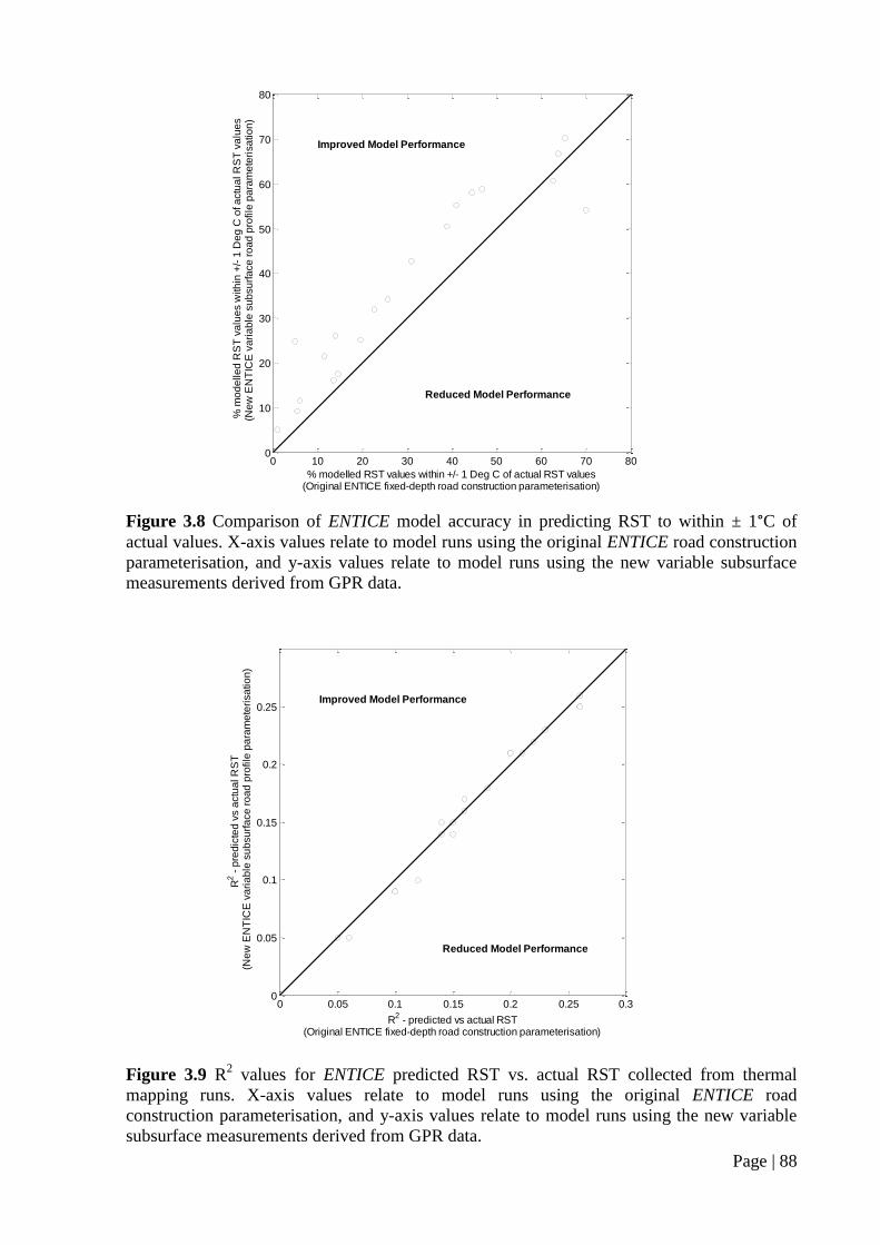
Page | 88
0 10 20 30 40 50 60 70 800
10
20
30
40
50
60
70
80
% modelled RST values within +/- 1 Deg C of actual RST values(Original ENTICE fixed-depth road construction parameterisation)
% m
od
elle
d R
ST
va
lue
s w
ith
in +
/- 1
De
g C
of a
ctu
al R
ST
va
lue
s(N
ew
EN
TIC
E v
ari
ab
le s
ub
su
rfa
ce
ro
ad
pro
file
pa
ram
ete
risa
tio
n)
Improved Model Performance
Reduced Model Performance
Figure 3.8 Comparison of ENTICE model accuracy in predicting RST to within ± 1°C of
actual values. X-axis values relate to model runs using the original ENTICE road construction
parameterisation, and y-axis values relate to model runs using the new variable subsurface
measurements derived from GPR data.
Figure 3.9 R2 values for ENTICE predicted RST vs. actual RST collected from thermal
mapping runs. X-axis values relate to model runs using the original ENTICE road
construction parameterisation, and y-axis values relate to model runs using the new variable
subsurface measurements derived from GPR data.
0 0.05 0.1 0.15 0.2 0.25 0.30
0.05
0.1
0.15
0.2
0.25
R2 - predicted vs actual RST
(Original ENTICE fixed-depth road construction parameterisation)
R2 -
pre
dic
ted
vs a
ctu
al R
ST
(Ne
w E
NT
ICE
va
ria
ble
su
bsu
rfa
ce
ro
ad
pro
file
pa
ram
ete
risa
tio
n)
Reduced Model Performance
Improved Model Performance

Page | 89
Hence, with the new variable subsurface measurements the overall accuracy of the ENTICE
model has improved significantly (Figure 3.8) with the Pm values increasing on 90% of the
study nights, and by up to 20% on individual nights. This suggests that the variable depth
profiles calculated from GPR measurements provide a more realistic representation of the
subsurface road construction around the study route than was attainable with the original
parameterisation proposed by Chapman et al. (2001b), enabling ENTICE to more accurately
model the thermal memory of the road surface at each forecast point. The new subsurface
measurements alone, however, appear to provide insufficient spatial data to increase the
overall amount of RST variability which is accounted for by the model.
Whilst the focus of this study is on the ENTICE model, it is important to emphasise that the
methodologies used in parameterising subsurface layer depths from GPR measurements
would be compatible with other surface energy balance models, and it is envisaged that such a
methodology could be used to integrate a spatial component into the existing heat conduction
module of the METRo model (Crevier & Delage 2001). In its current format METRo uses
standard XML code for all data input (Figure 3.10), enabling the subsurface layer depths
calculated from the inflexion point algorithm to easily be integrated into the model.

Page | 90
Figure 3.10 Sample METRo model code displaying the existing road layer parameterisation,
into which the new subsurface layers depths derived from GPR data could easily be added.
Source – METRo repository http://gna.org/projects/metro/
CHAPTER THREE SUMMARY
A study route was surveyed using GPR in an attempt to ascertain high resolution subsurface
road profile measurements to improve road construction parameterisation in the ENTICE
model. GPR has been shown to have considerable skill in objectively locating both major and
minor bridge decks around a route, all of which produce thermal singularities that have
implications for winter maintenance. The depths of subsurface layer interfaces around the
study route have been estimated via an inflexion point algorithm designed to identify
significant inflexions in the electromagnetic waveform of raw GPR trace data. Calculated
depths are then used to estimate subsurface temperatures and the subsurface heat flux at each
forecast point. A statistical analysis on road construction parameterisation has revealed an
increase of almost 7% in the overall percentage of modelled forecast values within ± 1°C of
the actual values, indicating a significant improvement in the spatial forecasting ability of the
ENTICE model as a result of the new re-parameterised road construction measurements.

Page | 91
4. SPATIAL RE-PARAMETERISATION OF THE
ENTICE MODEL: PART 2 – SURFACE ROUGHNESS
4.1 Surface Roughness
The roughness length parameter Z0 is a theoretical measure of the aerodynamic roughness of a
surface affecting the height at which the neutral wind profile near to the ground extrapolates
to zero (Oke 1992). Z0 is not a real, tangible quantity that can be measured, but is an artefact
of an equation structure. In practice, Z0 is determined from the least-square fitting of the
logarithmic velocity profile law (Equation 4.1) using wind profile data, or by graphically
plotting z versus U and extrapolating down to the level where U = 0, with its intercept on the
ordinate axis being ln Z0 (Arya 1988).
(
) (
) (4.1)
Estimation of Z0 at site specific locations within regions of inhomogeneity can be difficult. At
any site specific location, Z0 is related to the height of the surface elements and is a function
of the shape and density of the elements at that location and within the upwind “effective
fetch” or source area. However, the detailed resolution of individual patches comprising an
inhomogeneous surface (e.g., buildings, trees, agricultural patchwork, etc.) means that the
spatial resolution of turbulent exchanges of heat, mass and momentum is generally not known
at all or only vaguely guessed at (Schmid 1994). As a result, practical estimation of Z0 at a
specific locality is often based on published values for roughness of similar terrain elsewhere
(Wieringa et al. 2001). These values, which are usually ordered according to terrain type,
typically vary over five orders of magnitude from 10-5
m for smooth water surfaces to several
meters for forests and urban areas. A detailed review of roughness data derived from
boundary layer experiments conducted in the 1970s and 1980s was undertaken by Wieringa

Page | 92
(1993), who found that the Davenport (1960) classification of effective terrain roughness most
reliably described the effective roughness of realistic landscape types. This original
classification has since been updated at both ends of the roughness scale (Wieringa 1992;
Wieringa et al. 2001), providing one of the most thorough field-validated roughness
classifications to date (Table 4.1).
Table 4.1 Updated Davenport classification of terrain roughness (Wieringa et al. 2001)
Z0 (m) Landscape Description
1. 0.0002
“Sea”
Open sea or lake (irrespective of wave size), tidal flat, snow-covered flat
plain, featureless desert, tarmac and concrete, with a free fetch of several
kilometres.
2. 0.005
“Smooth”
Featureless land surface without any noticeable obstacles and with
negligible vegetation; e.g. beaches, pack ice without large ridges, marsh
and snow-covered or fallow open country.
3. 0.03
“Open”
Level country with low vegetation (e.g. grass) and isolated obstacles with
separations of at least 50 obstacle heights; e.g. grazing land without wind
breaks, heather, moor and tundra, runway area of airports. Ice with ridges
across-wind.
4. 0.10
“Roughly Open”
Cultivated or natural area with low crops or plant covers, or moderately
open country with occasional obstacles (e.g. low hedges, isolated low
buildings or trees) at relative horizontal distances of at least 20 obstacle
heights.
5. 0.25
“Rough”
Cultivated or natural area with high crops or crops of varying height, and
scattered obstacles at relative distances of 12 to 15 obstacle heights for
porous objects (e.g. shelterbelts) or 8 to 12 obstacle heights for low solid
objects (e.g. buildings).
6. 0.5
“Very Rough”
Intensively cultivated landscape with many rather large obstacle groups
(large farms, clumps of forest) separated by open spaces of about 8
obstacle heights. Low densely-planted major vegetation like bushland,
orchards, young forest. Also, area moderately covered by low buildings
with interspaces of 3 to 7 building heights and no high trees.
7. 1.0
“Skimming”
Landscape regularly covered with similar-size large obstacles, with open
spaces of the same order of magnitude as obstacle heights; e.g. mature
regular forests, densely built-up area without much building height
variation.
8. ≥ 2.0
“Chaotic”
City centres with mixture of low-rise and high-rise buildings, or large
forests of irregular height with many clearings.

Page | 93
4.2 Existing Z0 Parameterisation in ENTICE
It has been observed empirically that the wind speed over a surface increases logarithmically
with height under neutral stability. Some air molecules close the surface collide and stick to
the surface, whilst others bounce off in the direction from which they came and collide with
other air molecules moving in the direction of the wind, causing what is commonly known as
turbulent shear. The layer in which this turbulent shear has an effect is referred to as the
boundary layer, and the height of this layer depends upon the wind speed and Z0. In the
ENTICE model, Z0 is used both to influence the height of the boundary layer through the
calculation of an atmospheric damping depth, and also to calculate the exchange of heat
between the surface and the air (i.e. sensible heat flux (H)) through the use of a stability
correction factor that relies on a logarithmic form of the Richardson number.
In view of the fact that the height at the top of the boundary layer is likely to vary day by day,
Outcalt (1972) introduced the idea of an atmospheric damping depth (Z2) that corresponds to
the height at which the thermal diffusivity (Equation 4.2), which increases with height,
becomes greater than the bulk adiabatic diffusivity (Equation 4.3) which decreases with
height. The solution occurs at the depth where the declining bulk diffusivity is smaller than
the thermal diffusivity and is estimated through an iterative solution where the damping depth
is increased in 1 cm increments starting at Z0, i.e.
(4.2)
(4.3)
Solution at:
where Z2 is the atmospheric damping depth (i.e. height at which d > d’), k is von Karman‟s
constant, Uz is the wind speed at height Z, t is a time increment (a step function for the

Page | 94
estimation of the penetration depth of a 12-hour thermal disturbance) and Z0 is the roughness
length.
The exchange of heat between the surface and the air (H), as given in Equation (1.4), can be
expanded to give the following expression for H which includes a stability correction factor
R:
( )
(4.4)
where k is von Karman‟s constant, Uz is the wind speed at the boundary layer top (Z2), ρ is air
density, Z0 is the roughness length, Cp is the specific heat of air at constant pressure, T2 is the
air temperature at Z2, is the dry adiabatic lapse rate, T0 is the surface temperature, and R is a
stability correction factor (1 – Ri)1/2
, where Ri is Richardson‟s number and is the adiabatic
exchange coefficient for atmospheric stability.
In the ENTICE model, Z0 influences the sensible heat flux to air (H) by altering a logarithmic
form of the Richardson number (Equation 4.5) given by Outcalt (1972) which is used to
adjust the adiabatic exchange coefficient ( ) for atmospheric stability. The exchange
coefficient used at each iteration of ENTICE is the product of the adiabatic coefficient and the
stability correction factor R, i.e.
correction factor R = | |
[ ]
[ ]
(4.5)
where g is acceleration due to gravity, Uz is the wind speed at height Z, T bar is the mean
temperature gradient between the surface and the upper measurement level (Z2), Tz is the
temperature at height Z, T0 is the surface temperature and Z0 is the roughness length.
The ENTICE model uses the stability correction factor R such that if Ri is negative (i.e.
unstable conditions), the correction factor R is greater than unity and H is increased.

Page | 95
Conversely, if Ri is positive (i.e. stable conditions), R is less than unity and H is reduced.
From the equation structure of H, the greater the value of Z0 used in the ENTICE model, the
greater the value of H calculated.
Z0 is varied in ENTICE with respect to the ordinal land use and road type classifications in the
model. In the original site specific forecast model, Thornes (1984) made the estimate that Z0
would be approximately 15 cm due to the effect of moving traffic. Previous estimates of Z0
for roads were smaller than this and ranged from 0.5 cm (Nysten, 1980; cited in Thornes
(1984)) to 6 cm (Greene, 1980; cited in Thornes (1984)), but these estimates were based on
the assumption of no traffic. Indeed, if the wind is blowing parallel with a traffic free road
then Z0 values less than 1 cm could be feasible. However, with a continuous presence of
traffic assumed, Thornes (1984) suggested a Z0 value more appropriate to an urban
environment should be used, and selected a value of 15 cm which lies towards the lower end
of the urban roughness scale. This estimate related to a single site specific location (rural
motorway), unlike ENTICE which requires estimates of Z0 at any location. To overcome this
problem, Chapman (2002) created a look-up table of Z0 values assimilated from the scientific
literature (Table 4.2), providing typical estimates of how Z0 varies with respect to the ordinal
land use and road type classifications.
Table 4.2 Z0 values (cm) currently used in the ENTICE model in relation to the ordinal land
use and road type classification (modified from Chapman (2002) to account for an additional
„semi-rural‟ land use class).
Motorway A-Road B-Road C-Road
City Centre 200 200 200 200
Urban 100 100 100 100
Suburban 75 75 75 75
Semi-rural 50 50 50 50
Rural 50 25 25 25

Page | 96
The use of an ordinal Z0 dataset based on land use and road type classifications is a major
oversimplification. Such values fail to account for variations in static surface elements
(buildings, trees, etc.) within land use classes, and they take no account of wind direction and
the associated surface elements within the upwind fetch of a specific forecast point. Hence,
the existing method of Z0 parameterisation in ENTICE requires further improvement.
4.3 New Methodology for Z0 Estimation in ENTICE
4.3.1 Roughness length estimation
The roughest surfaces are typically found in urban areas, creating complex flow patterns that
characterise the atmospheric surface layer. The roughness of a surface has major implications
for surface drag, aerodynamic conductance for momentum transport, the depths of the
roughness layer and Ekman layer, wind speed and the shape of the wind profile, and the flow
type found in the urban canopy layer (Grimmond & Oke 1999). Knowledge of the
aerodynamic characteristics in urban areas is essential for describing, modelling and
forecasting the behaviour or urban flow patterns, but detailed field observations are seldom
available, thus requiring model simulations that in the majority of cases are not based directly
on observed measurements at the locality of interest (Tieleman 2003).
The roughness length parameter Z0, used as a theoretical measure of the aerodynamic
roughness of a surface, is commonly estimated using one of two approaches defined by
Grimmond & Oke (1999). The first of these is morphometric methods that utilise algorithms
relating aerodynamic parameters to measures of surface morphometry, whilst the second is
micrometeorological methods that use field observations of wind or turbulence to solve for
aerodynamic parameters included in theoretical relations derived from the logarithmic wind
profile (Grimmond & Oke 1999). Aside from the expense and difficulty involved in obtaining
and operating a field site, a major disadvantage of micrometeorological methods is that even

Page | 97
with the best available instrumentation, appropriate wind conditions for all directions are
rarely found during a field experiment and the natural heterogeneity of urban sites combined
with the sensitivity of analyses to small errors can result in unreliable measurements (Schaudt
1998). Morphometric methods on the other hand have the advantage that estimates of surface
roughness can be obtained without the need for expensive on-site instrumentation, but most
morphometric methods are based on empirical relations derived from wind tunnel work where
the simulation of flow rarely mimics the true conditions found in real world situations, where
wind direction is ever changing and the shape and density of roughness elements are not
regular.
As a prerequisite any method of Z0 estimation for use in road weather modelling should be
practically simple and cost effective to implement given the budgetary constraints that the
road weather industry is rapidly becoming accustomed with. Given the extensive geographical
areas over which road weather forecasting is required, the use of micrometeorological
methods requiring expensive on-site instrumentation can be ruled out in favour of a
morphometric method. Grimmond & Oke (1999) provide a detailed critical review of several
morphometric methods which the authors split into three main categories, a simple height
based approach, methods that use height and plan areal fraction, and methods that consider
height and frontal area index. Estimates of Z0 using these methods were compared with values
obtained from analysis of wind and turbulence observations based on a survey of
approximately 60 field studies and 14 laboratory studies of real and scale model cities. Over
the range of morphometric conditions found, the results provided no objective bias for
selecting one morphometric method over another, but when considering factors such as ease
of implementation, applicability across the full range of typical urban morphometries, and
conformity with suggested curves and envelopes of reasonableness, morphometric methods
that consider height and frontal area index were most favoured by the authors (Grimmond &
Oke 1999). In particular, the height and frontal area index model presented by Bottema (1997)

Page | 98
was found to generate estimates of Z0 that best conformed to observed measurements, but this
method required the most demanding set of input requirements of all the morphometric
methods. On the other hand, the simple height based approach is very simple to implement
within a GIS environment and was found to work well in the mean, but because its
formulation includes no recognition of density it fails to respond to the effects of packing and
increasingly overestimates roughness at very high and low densities (Grimmond & Oke
1999).
Hence, there are clearly benefits and drawbacks to each method, and given the lack of any
objective bias for selecting one morphometric method over another, one can argue that this
choice should relate to the specific requirements of the application, which is this instance is
road weather forecasting. As described in section 4.2, current estimation of Z0 in road weather
models is based on a fixed ordinal dataset of roughness values which has a number of
limitations already discussed. The main objective for re-parameterising Z0 in the ENTICE
model is to remove the reliance of the model on this ordinal classification in favour of a
continuous dataset of roughness values derived from some form of ground observation. As a
proof of concept, the use of a simple height based morphometric approach which will be
simple to implement within even the most basic of GIS environments provides a suitable
starting point.
4.3.2 Height based rule of thumb
Chapman (2002) attempted to approximate Z0 at hundreds of site specific locations around a
route from fish-eye images using the assumption that Z0 can be approximated by the ratio
1/10 of the height of the surface elements (Oke 1992). However, this direct calculation
method was eventually abandoned due to difficulties in measuring the horizontal distance
from lens to object required in order to calculate the height of intrusion from the object (e.g.
buildings, trees, etc.) angle. The 1/10 ratio is based on a well-known simple rule of thumb for

Page | 99
estimating Z0 (Equation 4.6) whereby, to a first order, Z0 is related to the height of the surface
elements (ZH) by the empirical coefficient f0 derived from observation, i.e.
(4.6)
Both Garratt (1992) and Hanna & Chang (1992) estimate the value of f0 to be ~ 0.1, which is a
commonly quoted value for surfaces in general, and across the range of roughness values it
has been shown to yield reasonable values of Z0 (Grimmond & Oke 1999). Hence, this height-
based rule of thumb is used as the basis for testing a new Z0 estimation in ENTICE designed
to eliminate the current dependence of the model on the aforementioned ordinal based Z0
values and their associated limitations.
4.3.3 Local Z0 estimation from LIDAR data
The height-based rule of thumb (Equation 4.6) was applied to a Light Detection And Ranging
(LIDAR) height dataset of the West Midlands, UK, to provide local estimations of Z0 around
the Birmingham study route described in Chapter 2. The LIDAR dataset, obtained via the
Landmap Service (http://www.landmap.ac.uk/), included a 2 m horizontal resolution Digital
Terrain Model (DTM), providing elevation measurements of the natural terrain features, and a
2 m horizontal resolution Digital Surface Model (DSM), which together with the natural
terrain features included additional features such as buildings, vegetation and roads. Hence,
subtracting the DTM from the DSM produced a dataset containing height measurements at 2
m horizontal resolution of all surface objects, from which local Z0 estimations for each 2 m
grid cell were calculated by applying the simple height-based rule of thumb (Equation 4.6).

Page | 100
4.3.4 Calculating effective Z0
To account for the effect of upstream surface elements on the local Z0 values at each point
along the route, and the influence of the prevailing wind direction on the magnitude of this
effect, an effective roughness length (Z0eff
) similar to that used by Vihma & Savijärvi (1991)
was calculated for each 2 m grid cell from the areal average (denoted ⟨ ⟩) of all local Z0
estimations within set geometric areas spanning away from each grid cell to a specified
distance of upwind fetch, i.e.
⟨ ⟩ (4.7)
The distance of upwind fetch used to calculate surface roughness at a point source will relate
to the source area or „footprint‟ within which the shape and density of the surface elements
has an influence on the localised flow at the point source where surface roughness is to be
estimated. In a study by Heilman et al (1989), several Bowen-ratio systems deployed at a
range of fetch to height ratios downwind of a change in surface roughness found that under
small Bowen ratio measurements (e.g. night-time), ratios of fetch to measurement height as
small as 20:1 can provide acceptable accuracy. This is considerably lower than the commonly
recommended ratio of 100:1 (Gash 1986; cited in Horst 1999), or even 250:1 as suggested by
Bottema (1997), and serves to show the uncertainty that exists in accurately determining an
„optimum‟ distance of upwind fetch to include in surface roughness estimation. Horst & Weil
(1994) used model estimates of the flux footprint to examine the fetch requirements for
accurate micrometeorological measurement of surface fluxes of passive, conservative scalars
within the surface flux layer, and found fetch to be a strong function of atmospheric stability.
Stable conditions were found to require a much greater fetch than unstable conditions, and the
fetch required even under moderately stable conditions was found in many cases to be
considerably greater than the commonly used rule of thumb of an upwind fetch equal to 100
times the measurement height (Businger 1986).

Page | 101
Table 4.3 shows values for minimum fetch computed using Equation 4.8 (ASCE, 1996),
which is derived from the early work of Brutsaert (1982) in providing theoretical
considerations of boundary layer development for use in estimating minimum fetch
requirements as a function of surface roughness. Equation 4.8 estimates xf for near neutral
conditions, requiring the exponent (0.14) to be increased for situations of increasing stability
and decreased for situations of increasing instability (ASCE, 1996).
(
)
(4.8)
where xf is the minimum fetch distance required for complete boundary layer development
(m), z is the maximum sensor height above the ground (m), d is the zero plane displacement
(m), and Z0m is the momentum roughness height of the surface (m).
Table 4.3 Minimum recommended upwind fetch distances (m) for various types of surface
cover, derived from Equation 4.8 (ASCE, 1996).
Height and type of surface cover z = 1 z = 2 z = 3 z = 12
0-0.0001m Water 180 400 630 3000
0.12m Grass 80 190 300 1500
0.5m Alfalfa 45 130 220 1200
1.5m Cattails n/a 60 140 950
10m Dense Trees n/a n/a n/a 320
The values for minimum fetch shown in Table 4.3 indicate that Equation 4.8 follows the
100:1 rule for a relatively wide range of vegetation and heights. However, since stable
conditions are shown in the literature to require much greater fetch than unstable conditions,
and since stable conditions are the most important conditions from a road weather modelling
perspective in relation to the potential for ice formation, an upwind fetch in the order of

Page | 102
1:250, which Bottema (1997) suggests is required for reasonable roughness estimates, is used
in the following analysis.
Based on the local Z0 values calculated for each forecast point along the Birmingham study
route using Equation 4.6, an upwind fetch ratio of 1:250 would require a fetch of 500 m to
ensure inclusion of the upper fetch threshold within the analysis. To determine whether a 500
m fetch would provide representative Z0eff
values, Kruskal-Wallis rank order tests (Dytham
1999) and Wilcoxon rank-sum tests were used to compare five LIDAR based Z0eff
datasets,
calculated for five distances of upwind fetch (100, 150, 200, 250 and 500 m), against an urban
land use classification (OWEN) derived by Owen et al (2006) for the UK West Midlands
metropolitan area (Figure 4.1). Each of the five roughness datasets were calculated assuming
a prevailing westerly wind direction (247.5 - 292.5°) typical of the study locality (Figure 4.2).
The OWEN land use dataset consists of eight land use classes at 1 km2 resolution
(villages/farms, suburban, light suburban, dense suburban, urban/transport, urban, light
urban/open water and woodland/open land) derived from dimensionality reduction of 25
spatial land-cover attributes using principal components analysis. Using the assumption that
surface roughness will vary significantly between each of the OWEN land use classes, the
most representative Z0eff
values for the study route will be those that vary the most, and hence
show the most significant differences, between land use classes.

Page | 103
Figure 4.1 Eight land use classes around the study route as defined by the OWEN land use
classification (Owen et al. 2006).

Page | 104
Figure 4.2 Illustration of effective roughness length (Z0eff
) calculation for each 2 m LIDAR
grid cell over distances of upwind fetch ranging from 100 m up to 500 m, assuming a westerly
prevailing wind.
Kruskal-Wallis is the non-parametric equivalent of a one-way analysis of variance (ANOVA)
and is used when a dataset violates the ANOVA assumptions about normality and
homogeneity of variance. Levene‟s test for homogeneity of variance produced highly
significant values (p-value < 0.001) for all five roughness datasets, indicating that significant
differences exist in the variances of the Z0eff
values between the land use groups. Thus,
Levene‟s null hypothesis of equal group variances was rejected and the Kruskal-Wallis test,
which makes no assumptions about homogeneity of variance or normal distributions, was
selected for analysis. The Kruskal-Wallis test is employed with rank-order data whereby the
raw data is converted to a rank in the overall dataset (Sheskin 2007), with the lowest value
obtaining a rank of 1. Hence, for each of the five roughness datasets the lowest Z0eff
value is

Page | 105
assigned a rank of 1, the next lowest value a rank of 2, and so on until every value in the
dataset is assigned a rank. The ranked samples are then returned to their original land use
groupings and a mean rank calculated for each group. If the result of the Kruskal-Wallis test is
significant, it indicates there is a significant difference between at least two of the land use
group mean ranks, and hence a significant difference in the Z0eff
values between these land use
classes.
The results from the Kruskal-Wallis analyses were highly significant (p < 0.001) over all five
distances of fetch (Table 4.4). This indicates that significant differences exist in the Z0eff
values between at least two of the land use classes for all five distances of fetch, but Kruskal-
Wallis tests do not reveal where these differences occur. Hence, for all five roughness datasets
post-hoc Wilcoxon rank-sum tests (Table 4.5) were performed on the Z0eff
values within each
independent land use class, comparing each class against each other to reveal where the
significant differences occur.

Page | 106
Table 4.4 Kruskal-Wallis results for Z0eff
comparisons between OWEN land use classes
N Mean Rank N Mean Rank N Mean Rank N Mean Rank N Mean Rank
OWEN 1. Villages/farms 463 668.32 461 645.84 460 606.58 458 586.3 447 580.73
Land use 2. Suburban 534 1035.19 534 1088.43 534 1107.03 534 1125.84 534 1102.76
3. Light suburban 125 1079.15 125 995.38 125 1010.3 125 1018.55 125 1103.52
4. Dense suburban 123 848.68 123 775.21 123 775.56 123 779.85 123 644.34
5. Urban/transport 341 1755.18 341 1808.78 341 1837.63 341 1851.92 341 1851.89
6. Urban 489 1008.56 489 949.89 489 934.92 489 915.41 489 927.37
7. Light urban/open water 42 1351.67 42 1567.95 42 1643.5 42 1637.5 42 1614.83
8. Woodland/open land 5 504.8 5 479 5 288.8 5 204.4 5 43
Total 2122 2120 2119
Chi-Square (Z0)
df (Z0)
Sig. (Z0)
Fetch (m) 100 150 200 250 500
660.867 799.676 900.591 954.626 988.674
7 7 7 7 7
0.000 0.000 0.000 0.000 0.000

Page | 107
Table 4.5 Wilcoxon P-values matrices comparing Z0eff
values between each OWEN land use class over five distances of upwind fetch
Land Use 1 2 3 4 5 6 7 8 1 2 3 4 5 6 7 8 1 2 3 4 5 6 7 8
1 0.000 0.000 0.000 0.000 0.000 0.000 0.751 0.000 0.000 0.000 0.000 0.000 0.000 0.468 0.000 0.000 0.000 0.000 0.000 0.000 0.730
2 0.000 0.212 0.000 0.000 0.261 0.000 0.019 0.000 0.102 0.000 0.000 0.000 0.000 0.008 0.000 0.052 0.000 0.000 0.000 0.000 0.001
3 0.000 0.212 0.001 0.000 0.048 0.032 0.049 0.000 0.102 0.000 0.000 0.162 0.000 0.023 0.000 0.052 0.000 0.000 0.017 0.000 0.005
4 0.000 0.000 0.001 0.000 0.000 0.000 0.017 0.000 0.000 0.000 0.000 0.000 0.000 0.027 0.000 0.000 0.000 0.000 0.000 0.000 0.001
5 0.000 0.000 0.000 0.000 0.000 0.000 0.000 0.000 0.000 0.000 0.000 0.000 0.000 0.000 0.000 0.000 0.000 0.000 0.000 0.000 0.000
6 0.000 0.261 0.048 0.000 0.000 0.000 0.008 0.000 0.000 0.162 0.000 0.000 0.000 0.004 0.000 0.000 0.017 0.000 0.000 0.000 0.001
7 0.000 0.000 0.032 0.000 0.000 0.000 0.002 0.000 0.000 0.000 0.000 0.000 0.000 0.000 0.000 0.000 0.000 0.000 0.000 0.000 0.000
8 0.751 0.019 0.049 0.017 0.000 0.008 0.002 0.468 0.008 0.023 0.027 0.000 0.004 0.000 0.730 0.001 0.005 0.001 0.000 0.001 0.000
Land Use 1 2 3 4 5 6 7 8 1 2 3 4 5 6 7 8 Land Use Classification
1 0.000 0.000 0.000 0.000 0.000 0.000 0.290 0.000 0.000 0.000 0.000 0.000 0.000 0.002 1: villages/farms
2 0.000 0.016 0.000 0.000 0.000 0.000 0.000 0.000 0.902 0.000 0.000 0.000 0.000 0.000 2: suburban
3 0.000 0.016 0.000 0.000 0.002 0.000 0.001 0.000 0.902 0.000 0.000 0.000 0.000 0.000 3: light suburban
4 0.000 0.000 0.000 0.000 0.000 0.000 0.000 0.000 0.000 0.000 0.000 0.000 0.000 0.000 4: dense suburban
5 0.000 0.000 0.000 0.000 0.000 0.000 0.000 0.000 0.000 0.000 0.000 0.000 0.000 0.000 5: urban/transport
6 0.000 0.000 0.002 0.000 0.000 0.000 0.000 0.000 0.000 0.000 0.000 0.000 0.000 0.000 6: urban
7 0.000 0.000 0.000 0.000 0.000 0.000 0.000 0.000 0.000 0.000 0.000 0.000 0.000 0.000 7: light urban/open water
8 0.290 0.000 0.001 0.000 0.000 0.000 0.000 0.002 0.000 0.000 0.000 0.000 0.000 0.000 8: woodland/open land
OWEN 100m Fetch OWEN 150m Fetch OWEN 200m Fetch
OWEN 250m Fetch OWEN 500m Fetch

Page | 108
To account for the problem of inflated error rates when conducting multiple Wilcoxon tests,
the Bonferroni Correction factor was applied to the standard 95% significance level, giving a
new independent test level of 99.8% (0.002). Without this correction factor, the probability of
rejecting the null hypothesis when it is actually true (Type 1 error) for at least one comparison
increases from 5% to 76% (based on a total of 28 comparisons) when comparing all the land
use classes. The Wilcoxon p-values (Table 4.5) reveal that with a fetch of just 100 m, only
68% of the roughness comparisons between all the land use classes are statistically
significant, increasing to 75%, 86% and 93% for distances of 150, 200 and 250 m
respectively. With a fetch of 500 m, however, 96% of the roughness comparisons between the
land use groups are statistically significant. Hence, using the assumption that surface
roughness is significantly different between each of the land use classes, then an upwind fetch
of 500 m produces Z0eff
values that most accurately reflect these conditions.
It is accepted that the use of a pre-defined distance is a major oversimplification, since most
recommendations in the literature suggest the fetch requirement to be a function of obstacle
height. However, whilst a variable approach is feasible for ENTICE, a pre-defined distance
enabled the use of inbuilt neighbourhood functions within ArcMap and allowed a buffer equal
to the fetch distance to be created and used as an analysis mask around each forecast point,
significantly reducing the processing requirements on the LIDAR dataset. Therefore, using a
pre-defined fetch of 500 m, Z0eff
values at each forecast point were calculated for eight
prevailing wind directions categorised into 45° approach angles (Figure 4.3) using a focal
mean wedge neighbourhood function in ArcMap. The resulting Z0eff
dataset contained eight
possible Z0eff
values for each forecast point along the study route (1 for each wind direction),
the maximum values of which for each wind category are shown in Figure 4.3. The selection
of 45° approach angles corresponding to the eight wind directions shown in Figure 4.3 was
made partly to simplify analysis for a proof of concept study such as this, but largely because
reliable wind direction data for the entire study route was not available, with the data used

Page | 109
taken from an automatic weather station located some distance from the study route (see
section 4.4.2). It is acknowledged however that in a real forecasting situation much smaller
approach angles should ideally be used, together with higher resolution reliable wind direction
data which was not available for this study.
Figure 4.3 Variation in maximum Z0eff
values (cm) around the study route with approaching
wind direction.
The minimum range of the Z0eff
values in each wind category was manually forced to 15 cm.
Whilst some of the calculated Z0eff
values were significantly below this threshold, the
proposed technique fails to account for the increased turbulence and mixing caused by
moving traffic which would imply a boundary layer deeper than for an untrafficked road.
Hence, a lower threshold of 15 cm was set for the Z0eff
values in each wind category to
account for moving traffic, the same value used by Thornes (1984) to simulate the effect of
moving traffic on a rural motorway. The Z0eff
values obtained for the study route using this

Page | 110
new methodology are typical of the range of values we could expect from a look-up table of
roughness values such as the Davenport classification of terrain roughness (Table 4.1) given
the land use classes that the study route encompasses (Figure 4.1).
The of Z0eff
values around the route for the eight directions of upwind fetch (Figure 4.4 (a))
reveals large variations with wind direction in the urbanised city centre (> 40 SD) as one
might expect given the variety in the shape and density of surface elements in city centres.
Similar variations in surface roughness are also evident in the largely rural south-westerly
section of the route (Figure 4.4 (b)), where a forested area adjacent to the route appears to act
as a natural screen against any approaching winds from a predominantly northerly to westerly
direction. In contrast, other sections of the route show little variation in surface roughness
with wind direction, including some suburban and urban areas where the surface elements are
less dense and more uniform in height than in the city centre. Hence, the need to account for
various directions of upwind fetch in the estimation of surface roughness at each forecast
point for ENTICE has been demonstrated. To implement this in ENTICE, changes are
required to the Geographical Parameter Database used to drive the model, along with changes
to the meteorological input files and the coding of the model in order to provide a variable
roughness parameter for each forecast point based on the forecast wind direction at each time-
step in the model.

Page | 111
Figure 4.4(a) Standard deviation of Z0eff
values at each forecast point around the study route
over the eight wind directions shown in Figure 4.3 and (b) enlarged view of a rural section of
the study route, revealing a forested area acting as a natural screen to approaching northerly to
westerly winds. LIDAR data courtesy of the Landmap Service.
SD of Z0eff
(Jenks Natural Breaks
Classification)
(a)
Forested area
(b)
Larger variation in
Z0eff
values with
wind direction due
to screening effects
of forest

Page | 112
4.4 Changes to ENTICE to Enable Inclusion of Z0eff
4.4.1 Z0eff
values
The new LIDAR based Z0eff
values were appended to the existing ENTICE GPD for the study
route, consisting of a database file containing the geographical and road infrastructure data for
every forecast point around the study route (Figure 4.5). Eight columns of Z0eff
values were
appended to the GPD file, corresponding to the eight different upwind approach angles from
which the Z0eff
values at each forecast point were calculated. The GPD file was then fed into
the ENTICE model (Appendix 5) as a GPD array via a spatial iterative loop, with all eight sets
of Z0eff
values assigned to individual variables within the GPD array ready for automatic
selection based on the wind direction:
Figure 4.5 Excerpt from the ENTICE GPD database file, showing the new LIDAR based Z0eff
values appended to the end of the database.
4.4.2 Wind direction
The existing ENTICE model does not include wind direction within its meteorological input
parameters. Hourly wind direction data for the appropriate nights was obtained from the
Coleshill automatic weather station run by the UK Meteorological Office and accessed
through the BADC website (http://badc.nerc.ac.uk/home/index.html). The raw meteorological
input files for ENTICE are simple comma separated files, to which the hourly wind direction
data was added as an extra comma separated value at the end of each line:
EASTING NORTHING LATITUDE SVF ALTITUDE SLOPE ASPECT LANDUSE FC ZONORTH ZONEAST ZOEAST ZOSEAST ZOSOUTH ZOSWEST ZOWEST ZONWEST
398915.27 283025.83 52.45 0.89 186 3.20 259.70 2 3000 0.17 0.28 0.20 0.22 0.28 0.10 0.28 0.07
398916.34 281939.08 52.44 0.89 190 4.70 289.54 2 3000 0.16 0.15 0.20 0.22 0.10 0.10 0.12 0.14
398917.59 281521.96 52.43 0.96 195 3.14 300.07 2 3000 0.08 0.22 0.22 0.14 0.17 0.06 0.03 0.12
398917.70 281916.84 52.44 0.94 190 4.70 289.54 2 3000 0.15 0.15 0.19 0.22 0.11 0.09 0.11 0.14
398918.37 281893.48 52.44 0.97 189 4.74 264.81 2 3000 0.14 0.15 0.19 0.23 0.11 0.08 0.11 0.12
398919.04 281847.87 52.43 0.96 188 4.97 251.57 2 3000 0.12 0.16 0.19 0.23 0.12 0.08 0.13 0.08
398919.64 281546.43 52.43 0.97 195 3.14 300.07 2 3000 0.08 0.23 0.21 0.15 0.17 0.06 0.03 0.12
398920.04 283046.96 52.45 0.89 186 3.20 259.70 2 3000 0.17 0.27 0.19 0.23 0.28 0.10 0.26 0.08
398921.01 281569.79 52.43 0.96 193 3.34 329.04 2 3000 0.07 0.22 0.21 0.16 0.15 0.05 0.03 0.12

Page | 113
LOCATION,DATE,TIME,T,Td,WIND,Wx,CLOUD-COVER(OCTAS),CLOUD-BASE(FT),WDIR
BHAM1,'09/12/1999, 12:00:00',7,6.8,6.4,NONE,3,2500,200
BHAM1,'09/12/1999, 13:00:00',6.5,6,6,NONE,4,2500,210
BHAM1,'09/12/1999, 14:00:00',6,5.7,5.6,NONE,5,2500,210
BHAM1,'09/12/1999, 15:00:00',5.6,5.4,5.3,RA,6,2500,220
BHAM1,'09/12/1999, 16:00:00',5.6,5.3,5,RA,6,2500,220
BHAM1,'09/12/1999, 17:00:00',5.6,5.1,4,RA,7,2500,220
Figure 4.6 Excerpt from an ENTICE comma separated raw meteorological input data file,
showing the wind direction appended to the end of each row.
Wind direction data was then fed into the model along with the other meteorological
parameters as an additional array and the values were averaged linearly for the 20 minute
intervals between actual input values. With each iteration of the spatial loop, a temporal
iterative loop was run to enable the correct column of Z0eff
values to be selected based on the
wind direction at each iteration. Each iteration of the temporal loop corresponded to the next
20 minute wind direction data, whilst each iteration of the spatial loop corresponded to the
next forecast point along the route.
for all forecast points do
for each 20 minute interval do
if wind direction >= 337.5 or < 22.5
select the northerly Z0eff
database
else if wind direction >= 22.5 and < 67.5
select the north-easterly Z0eff
database
else if wind direction >= 67.5 and < 112.5
select the easterly Z0eff
database
else if wind direction >= 112.5 and < 157.5
select the south-easterly Z0eff
database
else if wind direction >= 157.5 and < 202.5
select the southerly Z0eff
database
else if wind direction >= 202.5 and < 247.5
select the south-westerly Z0eff
database
else if wind direction >= 247.5 and < 292.5

Page | 114
select the westerly Z0eff
database
else if wind direction >= 292.5 and < 337.5
select the north-westerly Z0eff
database
else select the westerly Z0eff
database
end if
end for
end for
4.5 Statistical Analysis of New Z0eff
Values
To test whether the newly calculated Z0eff
values improve the spatial forecasting performance
of ENTICE, a statistical analysis was conducted on 20 nights thermal mapping data for the
study route. During the analysis, all of the geographical parameters in the model, with the
exception of roughness length, were fixed spatially to default values, rather than running the
model in „quasi-operational‟ mode. As with the analyses undertaken in Chapter 3, fixing all
other geographical parameters spatially ensures any changes identified in the model forecast
are solely due to the change in surface roughness, allowing us to quantify the effect of surface
roughness changes alone on model performance. Again, the resultant forecast statistics (Table
4.6) are not providing a true measure of model performance but a reflection of model bias
caused by the spatial fixing of the geographical parameters. However, like with the road
construction analyses in Chapter 3, by running the model twice, first using the original ordinal
Z0 values (Table 4.2) and then using the re-coded model with the new Z0eff
values calculated
from the LIDAR data, changes in the model results between the two model runs can be
identified, enabling us to quantify the impact of surface roughness changes on model
performance. Forecast statistics for both model runs are summarised in Table 4.6.

Page | 115
Table 4.6 Forecast statistics from a statistical analysis on surface roughness in ENTICE, where all geographical variables in the model were held
constant with the exception of surface roughness
Analysis 1 – Existing ordinal Z0 values Analysis 2 – New Z0eff
values
Night RMSE Pm Prm R2 RMSE Pm Prm R
2
1 -0.24 0.98 1.01 71.92 72.89 0.14 -0.39 0.96 1.03 70.99 71.34 0.27
2 0.61 1.06 1.22 54.22 69.75 0.32 0.38 1.03 1.09 65.19 71.65 0.50
3 -0.79 1.28 1.50 52.94 57.54 0.29 -1.08 1.26 1.66 45.47 58.20 0.30
4 -0.11 0.92 0.93 74.48 72.36 0.28 -0.36 0.92 0.98 69.17 73.86 0.29
5 -0.97 1.45 1.74 58.20 56.66 0.31 -1.10 1.44 1.81 53.6 56.57 0.38
6 -0.73 1.45 1.63 60.77 54.22 0.31 -0.81 1.44 1.66 58.65 54.49 0.40
7 -0.75 1.57 1.74 49.45 51.84 0.30 -1.03 1.54 1.85 40.91 53.34 0.37
8 -0.06 0.87 0.88 76.25 75.90 0.18 0.09 0.89 0.90 74.97 76.12 0.24
9 -1.88 0.90 2.09 15.52 74.57 0.34 -1.92 0.93 2.14 15.52 72.93 0.17
10 -0.23 1.13 1.15 68.69 67.76 0.23 -0.24 1.13 1.16 68.60 67.58 0.42
11 -0.28 0.76 0.81 82.57 85.01 0.23 -0.48 0.74 0.88 78.06 85.23 0.30
12 1.14 1.39 1.8 30.74 59.40 0.23 1.04 1.39 1.73 32.95 59.40 0.37
13 -0.09 0.96 0.96 72.18 70.54 0.19 0.02 0.98 0.98 70.01 70.41 0.35
14 0.42 0.72 0.83 71.47 86.60 0.14 0.36 0.72 0.80 74.83 86.33 0.24
15 0.69 1.41 1.57 44.80 57.76 0.28 0.71 1.43 1.59 44.94 57.59 0.04
16 0.09 0.56 0.57 93.98 94.47 0.16 0.05 0.56 0.57 94.60 94.12 0.16
17 -0.21 1.22 1.24 61.26 59.93 0.08 -0.15 1.25 1.25 60.19 58.60 0.27
18 -1.22 1.09 1.63 40.78 67.58 0.18 -1.04 1.12 1.53 51.44 67.32 0.28
19 -1.19 0.55 1.31 33.92 91.91 0.17 -0.96 0.61 1.14 57.23 90.40 0.29
20 -1.13 0.91 1.45 44.67 75.19 0.35 -1.23 0.91 1.53 38.57 74.26 0.35
Average -0.35 1.06 1.30 57.94 70.09 0.24 -0.41 1.06 1.31 58.29 69.99 0.30

Page | 116
These statistics reveal that replacing the original ordinal Z0 values with the new Z0eff
values
has little impact on the overall RMSE of the route-based forecast. Hence, the magnitude of
any errors in the forecasts remains similar, even though the new Z0eff
values increase the
overall negative bias in the forecast. In terms of model accuracy, the overall Pm value
increases slightly (+ 0.35%) using the new Z0eff
values (Table 4.6 & Figure 4.7) with a range
over the 20 nights of -8.5% to +23%. Negligible change is observed (-0.1%) in the Prm
values.
Whilst such statistics are a good indicator of the spatial forecasting ability of a model, they are
nonetheless limited to a resolution of ±1°C, and can potentially ignore finer scale
improvements to a model. In the previous chapter an analysis of R2 values for modelled
versus predicted RST, which unlike the Prm values is not limited by temperature resolution,
revealed no overall change in the variability of RST accounted for by ENTICE when the new
re-parameterised GPR based subsurface road construction measurements were incorporated
into the model. The same analysis here based on changes made to the surface roughness
estimation in the model reveals a 6% increase in the variability of RST accounted for by
ENTICE with the new Z0eff
values (Table 4.6 & Figure 4.8). Hence, with the new LIDAR
based Z0eff
values the overall spatial forecasting performance of the ENTICE model is
improved, suggesting that the new Z0eff
values used in ENTICE provide a more realistic
representation of the turbulent heat transfer in the boundary layer close to the road surface
than was possible with the original ordinal Z0 values. Accordingly, with the new Z0eff
values
ENTICE is able to better predict thermal temperature variations around a route.

Page | 117
Figure 4.7 Comparison of ENTICE model accuracy in predicting RST to within ± 1°C of
actual values. X-axis values relate to model runs using the original ENTICE ordinal based Z0
values, and y-axis values relate to model runs using the new LIDAR based Z0eff
values.
Figure 4.8 R2 values for ENTICE predicted road surface temperature vs. actual road surface
temperature collected from thermal mapping runs. X-axis values relate to model runs using
the original ENTICE ordinal based Z0 values, and y-axis values relate to model runs using the
new LIDAR based Z0eff
values.
0 0.1 0.2 0.3 0.4 0.5 0.60
0.1
0.2
0.3
0.4
0.5
R2 - predicted vs actual RST
(Original ENTICE ordinal based roughness values)
R2 -
pre
dic
ted
vs a
ctu
al R
ST
(Ne
w E
NT
ICE
LID
AR
ba
se
d r
ou
gh
ne
ss v
alu
es)
Improved Model Performance
Reduced Model Performance
0 10 20 30 40 50 60 70 80 90 1000
10
20
30
40
50
60
70
80
90
100
% modelled RST values within +/- 1 Deg C of actual RST values(Original ENTICE ordinal based roughness values)
% m
od
elle
d R
ST
va
lue
s w
ith
in +
/- 1
De
g C
of a
ctu
al R
ST
va
lue
s(N
ew
EN
TIC
E L
IDA
R b
ase
d r
ou
gh
ne
ss v
alu
es)
Reduced Model Performance
Improved Model Performance

Page | 118
CHAPTER FOUR SUMMARY
A new method for de-parameterising surface roughness in route-based forecast models using
high resolution LIDAR data coupled with spatial processing techniques has been described.
The technique calculates an effective roughness length at each forecast point from the areal
average of all height based local Z0 estimations within defined areas spanning away from
each forecast point. The roughness values obtained have been implemented in the ENTICE
model, and a statistical analysis on surface roughness has revealed a 6% increase in the
variability of RST accounted for by ENTICE with the new re-parameterised surface
roughness measurements, despite there being negligible change in the overall Pm values
using this new technique. In the following chapter the integrity of the new re-parameterised
surface roughness and road construction measurements proposed in this thesis will be fully
tested through spatial validation of the ENTICE route-based forecast model using the new
cluster based validation strategy proposed in Chapter 2.

Page | 119
5. SPATIAL VALIDATION OF THE ENTICE ROUTE-
BASED FORECAST MODEL
When developing the validation technique outlined in Chapter 2 of this thesis, it was
envisaged that the technique could be used as a rapid integrity test for any future measurement
techniques that are designed to improve upon existing parameterisations within route-based
forecast models. This chapter aims to test this by verifying the integrity of the re-
parameterisations to surface roughness and road construction proposed in Chapters 3 and 4
using the new cluster based validation strategy proposed in Chapter 2. The new LIDAR based
Z0eff
values and subsurface road construction profiles provide the opportunity to replace the
existing categorical land use and road type parameterisations used in the original clustering
solutions with a much higher resolution continuous dataset derived from LIDAR and GPR
measurements.
5.1 Summary of Overall Model Performance
Prior to undertaking the cluster based validation strategy, an analysis of the entire route
statistics is required in order to prove the benefits of a cluster level analysis. With the ENTICE
model returned to a ‘quasi-operational’ (hence, true model performance) mode with all the
parameters within the model set to their best values, the model was re-run for all 20 nights
taking into account the new surface roughness and road construction parameterisations
identified in Chapters 3 and 4. These results were then compared to the original model runs
(Table 2.4) before any changes had been made to the model. Figure 5.1 displays the average
RMSE values for the modelled RST over the 20 nights, and shows a clear reduction in the
magnitude of any model errors when the re-parameterised surface roughness and road
construction measurements are introduced into the model. On 85% of the study nights the
RMSE of the forecast is reduced when model changes are introduced, with the overall average

Page | 120
for the 20 nights falling by 0.28°C from 1.48°C to 1.20°C. The overall spatial forecasting
ability of the model, as represented by the Pm values, has also improved significantly (Figure
5.2), increasing on 85% of the study nights when the model changes are introduced, with the
overall average for the 20 nights increasing from 46.94% (Table 2.4) to 60.93%. The three
nights where the spatial forecasting performance of the model appears to decrease were all
damped nights where thermal mapping is generally more susceptible to errors due to factors
such as increasing variability in surface emissivity. Emissivity in the ENTICE model is held at
a constant 0.95 which can introduce considerable error during a survey (Gustavsson 1999),
and such errors are often greatest on damped nights where road surface conditions are more
changeable. To overcome such errors, continued research is required into improving the
accuracy of the thermal mapping technique. The overall variability of RST accounted for by
ENTICE increases on 60% of the study nights when model changes are introduced (Figure
5.3), with an overall increase of 3% over the 20 nights. Those nights where the largest
decreases were found in the variability of RST accounted for by ENTICE were again damped
nights.
Analysis of model performance using entire route statistics has therefore shown that the
overall spatial forecasting ability of the ENTICE model has improved as a result of the re-
parameterisation of surface roughness and road construction within the model. As shown in
Chapter 2, however, the performance of a route-based forecast model can be better assessed
by analysing model statistics at a cluster level, since an entire route analysis can often mask
deficiencies (and improvements) in the spatial forecasting ability of the model. Cluster level
analyses also enable the consistency of new clustering solutions, and hence new measurement
techniques, to be tested via the calculation of clustering similarity coefficients. Such analyses
indicate the ability of clusters in capturing the physical relation between RST around a route
and the geographical and road infrastructure parameters used to create the cluster, and thus

Page | 121
provide a good integrity test for any new measurement techniques which alter a clustering
solution.
Figure 5.1 Average RMSE values for ENTICE predicted RST over the Birmingham study
route (20 nights). X-axis values relate to model runs before any changes were made to the
ENTICE model, and y-axis values relate to model runs which incorporate the re-parameterised
surface roughness and road construction measurements.
0 0.5 1 1.5 2 2.5 30
0.5
1
1.5
2
2.5
3
RMSE of ENTICE route based forecast model(Original ENTICE model forecast before any changes)
RM
SE
of E
NT
ICE
ro
ute
ba
se
d fo
reca
st m
od
el
(Ne
w E
NT
ICE
mo
de
l fo
reca
st a
fte
r a
ll m
od
el ch
an
ge
s)
Improved Model Performance
Reduced Model Performance

Page | 122
Figure 5.2 Comparison of ENTICE model accuracy in predicting RST to within ± 1°C of
actual values. X-axis values relate to model runs before any changes were made to the
ENTICE model, and y-axis values relate to model runs which incorporate the re-parameterised
surface roughness and road construction measurements.
0 10 20 30 40 50 60 70 80 90 1000
10
20
30
40
50
60
70
80
90
100
% modelled RST values within +/- 1 Deg C of actual RST values(Original ENTICE model forecast before any changes)
% m
od
elle
d R
ST
va
lue
s w
ith
in +
/- 1
De
g C
of a
ctu
al R
ST
va
lue
s(N
ew
EN
TIC
E m
od
el fo
reca
st a
fte
r a
ll m
od
el ch
an
ge
s)
Reduced Model Performance
Improved Model Performance
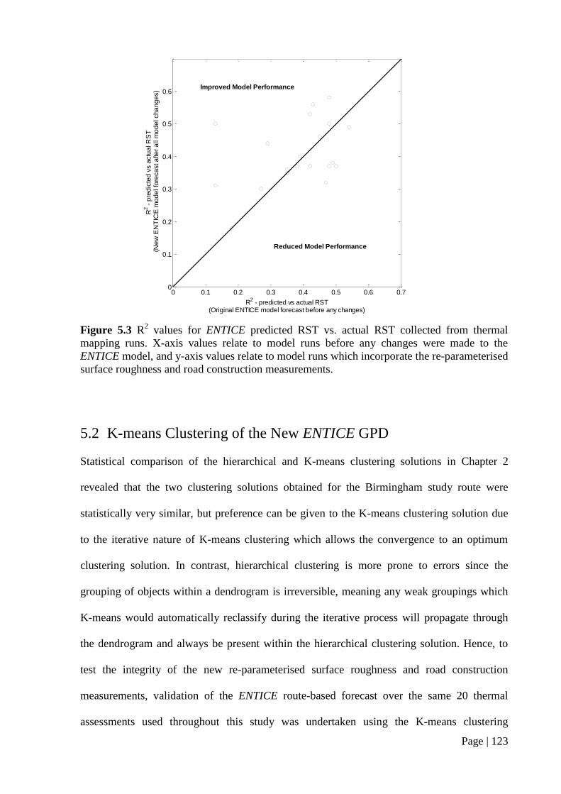
Page | 123
Figure 5.3 R2 values for ENTICE predicted RST vs. actual RST collected from thermal
mapping runs. X-axis values relate to model runs before any changes were made to the
ENTICE model, and y-axis values relate to model runs which incorporate the re-parameterised
surface roughness and road construction measurements.
5.2 K-means Clustering of the New ENTICE GPD
Statistical comparison of the hierarchical and K-means clustering solutions in Chapter 2
revealed that the two clustering solutions obtained for the Birmingham study route were
statistically very similar, but preference can be given to the K-means clustering solution due
to the iterative nature of K-means clustering which allows the convergence to an optimum
clustering solution. In contrast, hierarchical clustering is more prone to errors since the
grouping of objects within a dendrogram is irreversible, meaning any weak groupings which
K-means would automatically reclassify during the iterative process will propagate through
the dendrogram and always be present within the hierarchical clustering solution. Hence, to
test the integrity of the new re-parameterised surface roughness and road construction
measurements, validation of the ENTICE route-based forecast over the same 20 thermal
assessments used throughout this study was undertaken using the K-means clustering
0 0.1 0.2 0.3 0.4 0.5 0.6 0.70
0.1
0.2
0.3
0.4
0.5
0.6
R2 - predicted vs actual RST
(Original ENTICE model forecast before any changes)
R2 -
pre
dic
ted
vs a
ctu
al R
ST
(Ne
w E
NT
ICE
mo
de
l fo
reca
st a
fte
r a
ll m
od
el ch
an
ge
s)
Reduced Model Performance
Improved Model Performance

Page | 124
technique described in Chapter 2. As with the original analysis in Chapter 2, the ENTICE
model was run in ‘quasi-operational’ mode with all the parameters within the model set to
their best values, and the standard K-means clustering algorithm available within SPSS 16.0
for Windows® was used with the dataset again partitioned into 12 clusters based on Equation
2.4. Given that the Z0eff
values at each forecast point vary temporally based on the forecast
wind direction, the Z0eff
values associated with a westerly wind direction, which was the most
dominant wind direction over the 20 nights, were used in the clustering analysis to enable
comparison with the original K-means clustering solution.
Figure 5.4 displays a map of the new K-means clustering solution for the Birmingham study
route, together with a summary GPD showing the mean values of the geographical and road
infrastructure parameters within each cluster. Comparison of this new clustering solution with
the original K-means solution in Chapter 2 (Figure 2.6 (b)) reveals similarities within some of
the clusters. For example, clusters 5 and 6 in the new clustering solution (Figure 5.4) are
representative of forecast points located under bridges or underpasses, as indicated by the low
ψs values within these clusters, and they account for exactly the same forecast points as
clusters 3 and 7 in the original K-means clustering solution (Figure 2.6 (b)). Within these
clusters ψs is the most dominant parameter, so we would expect to see similarities in these
clusters given that the ψs measurement is the same in both clustering solutions. As with the
original K-means clustering solution (Figure 2.4 (b)) there is a lack of any single dominant
cluster, but the re-parameterisation of surface roughness and road construction within the
ENTICE model appears to have created subtle differences between the original and the new
K-means clustering solutions.

Page | 125
Cluster ψs Altitude Slope Sin
Aspect
Cos
Aspect
Z0eff
Conductivity
1 0.92 155 1.69 -0.23 0.72 21.79 0.00362
2 0.68 130 1.65 0.53 -0.13 87.49 0.00365
3 0.91 211 4.81 0.12 -0.08 20.38 0.00355
4 0.51 228 5.88 -0.87 -0.49 80.00 0.00400
5 0.13 148 1.96 0.77 -0.48 63.48 0.00380
6 0.17 192 2.18 -0.77 0.48 17.50 0.00349
7 0.87 129 1.81 0.81 -0.30 36.77 0.00378
8 0.94 192 2.14 0.86 -0.25 22.92 0.00374
9 0.94 192 4.45 -0.57 0.22 20.31 0.00402
10 0.90 164 1.48 0.34 0.76 25.57 0.00394
11 0.92 177 1.97 -0.19 -0.85 20.16 0.00376
12 0.93 217 3.03 -0.84 -0.28 88.00 0.00375
Figure 5.4 A map of the new K-means clustering solution for the Birmingham study route,
together with a summary GPD showing the mean values within each cluster.

Page | 126
A comparison of cluster 3 in the new K-means solution (Figure 5.4) with cluster 2 in the
original K-means clustering (Figure 2.6 (b)) reveals how both of these clusters represent
forecast points located at higher altitude, higher gradient rural parts of the study route where
the road construction appears to be shallower. This is indicated by the lower average road
thermal conductivity and Z0eff
values and the higher altitude and slope values within these
clusters. In both cases these clusters account for only a small proportion of the overall study
route. However, a reduction from 6% in the original clustering solution to 5.3% in the new K-
means solution provides an indication of the fine-tuning of clusters, which is evidenced by a
substantial increase in optimisation iterations during clustering, increasing from 16 iterations
in the original K-means clustering to 26 iterations in the new clustering solution in order to
reach the optimum solution. Hence, having replaced the existing ordinal road type and land
use data in ENTICE with new higher resolution continuous datasets derived from LIDAR and
GPR data, clusters of forecast points have been refined to account for greater variations in
surface roughness and road construction which are now accounted for in the ENTICE GPD.
Table 5.1 displays the standard set of route-based forecast validation statistics calculated for
each of the new K-means clusters, based on the same 20 thermal assessments of the study
route used throughout this study. Analysis of the overall entire route statistics has already
revealed a significant improvement in the overall forecasting ability of the ENTICE model as
a result of the new re-parameterised surface roughness and road construction measurements
within the model (Figure 5.1 to Figure 5.3). However, analysing the statistics in Table 5.1 at
the cluster level reveals further information regarding model performance.

Page | 127
Table 5.1 ENTICE route-based forecast validation statistics for the Birmingham study
route calculated for individual K-means clusters.
RMSE Pm Prm Forecast
Points
Entire Route
Original
-0.49
-1.06
0.89
0.86
1.20
1.48
60.93
46.94
79.35
79.56
2261
2261
Cluster 1 -0.34 0.57 0.93 70.18 92.52 305
Cluster 2 -1.63 0.77 1.84 27.54 84.03 211
Cluster 3 -0.53 0.85 1.19 61.46 87.54 120
Cluster 4 -0.11 0.00 0.57 95.00 100.00 1
Cluster 5 -0.95 1.60 1.99 33.70 48.48 23
Cluster 6 -2.70 1.42 2.96 20.00 55.00 2
Cluster 7 -0.86 0.69 1.30 52.00 86.61 310
Cluster 8 -0.31 0.62 0.95 68.51 92.19 404
Cluster 9 0.31 0.56 0.88 72.81 91.86 196
Cluster 10 -0.29 0.94 1.19 61.96 77.79 332
Cluster 11 -0.37 0.65 0.97 66.32 87.82 307
Cluster 12 -0.55 0.56 0.99 65.30 92.60 50
In 75% of the clusters in Table 5.1, the SD values are lower than the overall route statistic,
indicating that thermal variations are well represented by the new clustering solution. Eight
clusters in the new K-means clustering solution have RMSE values lower than the overall
route statistic, which together account for 75.9% of the entire study route. This compares to
seven clusters and 69.5% of the study route in the original K-means clustering solution,
indicating that the overall magnitude of errors around the study route has decreased as a result
of the new re-parameterised surface roughness and road construction measurements in the
ENTICE model. The clusters also reveal a large improvement in the overall spatial forecasting
ability of the model, with 75.9% of the entire study route (8 clusters) having a higher Pm
value than the overall route statistic of 60.93%. This represents an increase of 23.8% from the

Page | 128
original K-means clustering solution where a little over half of the study route (52.1%)
showed better spatial forecasting performance than the overall route statistic would otherwise
indicate. Analysis of the overall Prm values reveals little change from the original K-means
clustering solution, with the residual statistics in 9 out of the 12 clusters, which accounts for
84.2% of entire study route, significantly better than the entire route statistic of 79.35%.
The statistics in Table 5.1 also reveal areas where model performance needs to be improved.
The poorest performing clusters are clusters 2, 5 and 6. As previously mentioned, clusters 5
and 6 are representative of forecast points located under bridges or underpasses, locations
which the ENTICE model is known to be less accurate in forecasting for due to the lack of
any advective component in the zero-dimensional heat balance model which ENTICE uses.
From Figure 5.4 it can be seen that cluster 2 is representative of forecast points located mainly
in the city centre where ψs values are much lower, mainly due to the presence of tall buildings
in the city centre, and Z0eff
values are higher due to the increased drag imposed on the airflow
by the rough terrain in the city centre. This is comparable to cluster 9 in the original K-means
clustering solution (Table 2.4 (b) & Figure 2.6 (b)), where on average less than 10% of
modelled RST values were within ± 1°C of the actual values. With the new clustering solution
this has improved to over 27%, but it is still well below the entire route average. The large
negative bias of -1.63°C within this cluster suggests that the ENTICE model is failing to fully
account for the typical ‘urban heat island’ effect which is common to city centres. Canyon
geometry in city centres typically results in increased shading from solar radiation during the
day but increased heat retention throughout the night by blocking the escape of long wave
radiation from the surface and storing heat within the fabric of buildings. Also, levels of
traffic are generally higher in city centres and provide a major source of anthropogenic heat
(Smith et al. 2009) which further adds to this retention of heat in city centres. Whilst the
ENTICE model attempts to account for such factors the cluster statistics in Table 5.1 reveal
that further work is required with this aspect of model. Hence, validation of the ENTICE

Page | 129
route-based forecast model using clustering techniques has again been shown to provide a
much more representative measure of the model’s spatial forecasting ability. Without
validation at the cluster level, a simple analysis of the entire route statistics would have failed
to reveal these deficiencies in the model. Accordingly, validation at the cluster level should be
seen as the new minimum standard with which to verify route-based forecast models.
5.3 Consistency of the New K-means Clustering Solution
To further test the integrity of the new re-parameterised surface roughness and road
construction measurements in ENTICE, calculation of a new CSC dataset can be undertaken
using the new forecast data obtained from the re-runs of the ENTICE model which
incorporated the new Z0eff
values and subsurface thermal profiles. An improvement in the
CSC dataset for the same pairs of thermal mapping runs would indicate that the re-
parameterised surface roughness and road construction measurements help the clusters to
better capture the physical relation between measured RST around the study route and the
geographical and road infrastructure parameters used to cluster the data. The CSC analysis
was performed on the same pairs of thermal mapping runs as used in the original CSC
analysis in Chapter 2 (Table 2.5), giving a total of 9 comparisons (3 damped, 3 intermediate
and 3 extreme), the results of which are shown in Table 5.2.

Page | 130
Table 5.2 Clustering similarity coefficients (CSC) for independent pairs of thermal
mapping runs in the same weather category, calculated using the new K-means clustered
forecast points.
TM pairs No. of records No. of clusters CSC
Damped (1,2) 2261 12 0.58
Damped (1,3) 2261 12 0.83
Damped (2,3) 2261 12 0.75
Intermediate (1,2) 2261 12 1.00
Intermediate (1,3) 2261 12 1.00
Intermediate (2,3) 2261 12 1.00
Extreme (1,2) 2261 12 1.00
Extreme (1,3) 2261 12 1.00
Extreme (2,3) 2261 12 1.00
Results of the new CSC analysis reveal that the coefficients vary from 0.58 to 1.00 with a
mean over all weather categories of 0.91, which is the same as the mean coefficient value in
the previous CSC analysis (Table 2.6 (b)). For individual weather categories, a decrease in the
coefficient values under damped conditions occurs with the new clustering solution, but under
highly stable atmospheric conditions (extreme) when the accuracy of road weather forecasts is
most crucial, the coefficient values increase to a mean of 1.00 for the new K-means clustering
solution compared to an original mean of 0.95 for the extreme comparisons with the original
K-means clustering solution (Table 2.6 (b)). Hence, whilst the overall ability of the clusters in
capturing the physical relation between RST around the study route and the geographical and
road infrastructure parameters used to cluster the data has remained the same, on the extreme
nights when road weather forecasts need to be most accurate and factors such as road
construction and surface roughness have a greater influence on RST (Chapman et al. 2001b),
the refined clusters have been shown to better capture this relationship.

Page | 131
CHAPTER FIVE SUMMARY
Spatial validation of the ENTICE model has been undertaken using the new cluster based
validation technique proposed in Chapter 2. Statistical analysis of model performance using
entire route statistics has revealed an overall reduction in model error and a significant
increase in the overall spatial forecasting ability of the model. Integration of the new re-
parameterised road construction and surface roughness measurements into the ENTICE
model has led to subtle changes in the clustering solution for the study route and an increase
in optimisation iterations for the K-means clustering solution, which is symptomatic of cluster
refinement. On extreme nights when the accuracy of road weather forecasts is most crucial,
the refined clustering solution is shown to better capture the physical relation between RST
and the geographical and infrastructure parameters around the study route.
The new re-parameterised road construction and surface roughness measurements proposed
in this thesis have therefore passed the integrity test, but the cluster level statistics presented
in this chapter reveal further scope for improvement with the ENTICE model, particularly in
city centre locations where anthropogenic heat emissions are most prevalent. Vehicle
emissions provide a major source of anthropogenic heat in urban areas, but the ability to
parameterise the effects of traffic on the spatial variation of RST has continually proven to be
problematic in route-based forecasts. This will be considered in the following chapter where
a critique of the analysis techniques used in this thesis is provided along with suggestions for
future research within this field.

Page | 132
6. CRITIQUE AND SUGGESTED IMPROVEMENTS
This thesis has started to address some of the issues relating to the validation and
parameterisation of route-based forecast models, using the ENTICE route-based forecast
model as a case study. The spatial component of route-based forecast models such as ENTICE
has significantly increased the resolution of RST forecasts to the microclimatic level, but such
fine scale modelling of some of the geographical and road infrastructure parameters used to
drive the ENTICE model (Table 2.2) can be challenging. The work presented in Chapters 3
and 4 of this thesis has shown that progress is being made on this front, with basic ordinal
land use and road type parameterisations in the ENTICE GPD being replaced by much higher
resolution surface roughness and road construction measurements derived from LIDAR and
GPR data respectively. Whilst the validation statistics presented in this thesis have shown
significant improvements in model performance with the new re-parameterised surface
roughness and road construction measurements, they have also revealed that the ENTICE
model is by no means perfect, and that further improvements can be made. At each stage of
the research problems have been highlighted, and this chapter presents a summary of how this
project could be improved and makes recommendations for future research within this field.
6.1 Critique of Techniques
6.1.1 GPR road construction data
The integrity of the new re-parameterised road construction measurements presented in this
thesis ultimately depends upon the quality of the GPR data. In hindsight the use of a 250 MHz
antenna would have provided greater depth penetration than was achieved with a 500 MHz
antenna, and may have prevented the need to manually parameterise the bottom two layers of
the subsurface profile. The true quality of GPR data can only be fully assessed through road
core samples, but such an exercise is impractical at this scale so an alternative methodology is

Page | 133
required. As a starting point, a comparison of the same route using several radars from
different manufacturers would provide a good indication of data quality, but a shortage of
financial resources proved to be the main obstacle preventing such an analysis from being
undertaken. Indeed, the costs associated with obtaining GPR surveys are still relatively high,
but it is envisaged that these costs will come down over time and GPR data will become more
widely available.
Whilst the integration of GPR data into route-based forecasts provides an opportunity to
revolutionise the modelling of road construction in surface energy balance models, the whole
methodology of having to drive a route in order to obtain a subsurface GPR dataset could be
seen as a backwards step for route-based forecasting. Current advancements in shading and
sky view estimation using a fully GIS-based approach (Gal et al. 2007; Gal et al. 2009; Brown
et al. 2008a) suggest that route-based forecasting is rapidly moving towards a complete
desktop surveying solution, where forecast providers would no longer have to rely on mobile
surveying techniques to obtain the geographical and infrastructure data required for the spatial
component of a route-based model. An ideal scenario would see local authorities become
responsible by law for maintaining an up to date GPR database for their road network, with
this data made freely accessible to forecasting agencies as and when needed for
parameterising road construction in route-based forecast models. Indeed, some local
authorities (e.g. Neath Port Talbot) already hold GPR datasets for parts of their road network
(B Williams 2009, pers. comm., 3 Feb), which suggests that local authorities would be more
able to absorb the costs associated with this than a forecasting agency, and the data provided
would be useful for other applications beyond road weather forecasting such as structural
capacity estimation of roads and bridges to identify the remaining serviceable life of these
structures. Many roads nowadays can go for up to 10 years between resurfacing cycles, so it is
envisaged that a 5 year maximum update cycle for GPR surveys would be sufficient to ensure

Page | 134
most changes are documented within a reasonable time frame. Of course, the more frequent
this update cycle, the more accurate a GPR database will ultimately be.
The inflexion point algorithm used in this thesis (Appendix 2) to detect subsurface layer
interfaces in the electromagnetic waveform of the raw GPR traces relies on the basic
assumption that any inflexion in the waveform above a predefined amplitude is a subsurface
layer interface. Whilst for the majority of GPR traces this is the case, the algorithm fails to
account for potential anomalies in the electromagnetic waveform which can be caused by
objects such as utility pipes or drainage covers. By calculating an EWMA for the GPR
dataset, the effects of any such anomalies are minimised to some extent, but further research
aimed at improving the existing algorithm (or developing an new algorithm) to enable such
anomalies to be rapidly identified would be a valuable addition to this research.
6.1.2 LIDAR based Z0eff
values
The calculation of Z0eff
values using the methodology outlined in Chapter 4 has been shown to
increase the overall variability of RST accounted for in the ENTICE model by 6%, but the
methodology presented has a number of limitations. Whilst the inclusion of wind direction in
the estimation of Z0eff
values is a major step forward for the ENTICE model, the technique
fails to take into account wind speed. Ultimately this is a result of the real-time nature of the
forecast, which relies on the model having a pre-defined look-up table of Z0eff
values for each
forecast point. A potential improvement could involve the weighting of all LIDAR grid cells
for each forecast point, based on the distance of the cell from a given forecast point and the
forecast wind speed. Indeed, this highlights a further limitation of the proposed height based
technique, since in its current guise the technique assumes that every LIDAR grid cell within
the upwind fetch of a forecast point is an equal contributor to the surface roughness at the
forecast point. Equally, the technique only accounts for a constant direction of flow which is
normal to the face of the forecast point, whereas in reality wind direction (and speed) is ever

Page | 135
changing and, even if a street pattern is relatively regular, the size and shape of individual
roughness elements such as buildings and trees are not regular (Grimmond & Oke 1999).
Ultimately it is envisaged that the proposed technique could be further developed to allow for
a variable distance of upwind fetch at every forecast point, based not only on obstacle height
and wind speed but also on the active surface area presented to the oncoming flow such as the
frontal area index (Grimmond & Oke 1999) of the surface elements within the upwind fetch,
which could be approximated from LIDAR data.
The cost of LIDAR data has fallen recently to the extent that high resolution height data is
available to the academic community for as little as £1 per square kilometre through
commercial enterprises such as Bluesky International Limited (http://www.bluesky-
world.com/), although the costs to commercial companies are usually considerably higher.
Whether this proves to be an obstacle to the widespread use of LIDAR data in road weather
modelling remains to be seen, but recent work undertaken in Denmark to estimate shadowing
effects on RST using a high resolution LIDAR dataset known as the Danish Height Model
(Pedersen et al. 2010) is encouraging.

Page | 136
6.2 Traffic Parameterisation
Whilst this thesis has so far concentrated on improving the parameterisation of surface
roughness and road construction in the ENTICE model, traffic is a further parameter which is
currently not fully accounted for in the model. The re-parameterisation of road construction
and surface roughness in the ENTICE model means that the original road type and land use
parameterisations are no longer a requirement, and since the existing ENTICE traffic
parameterisation relies on these ordinal classifications (see section 6.2.2 for further details), a
new methodology for parameterising traffic is required. Modelling the effects of traffic on the
spatial variation of RST, however, has proven to be problematic in route-based forecasts,
largely due to the lack of detailed information regarding the spatial variation of traffic density
with time. Traffic information has traditionally been collected using inductive-loop detectors
embedded in the road or with video cameras. These fixed installations fail to provide any
traffic information beyond their installed locations, and their coverage is usually confined to
congestion-sensitive motorways and a limited number of tunnels, bridges and intersections
(Kristiansen et al. 2003).
6.2.1 Impacts of traffic on RST
Various studies have been undertaken over the past 25 years to assess the impact of traffic on
RST, and this impact is now reasonably well quantified and understood. Prusa et al. (2002)
identified several ways in which vehicles can modify RST, and these can be generally
grouped into three main categories; Heating, Shading and Motion. Heat can be added to the
road surface from the engine and exhaust via sensible heat and moisture fluxes (Figure 6.1
(a)) as well as frictional heat dissipation from the tyres (Figure 6.1 (b)) and braking. Vehicles
also have a dominant shading effect, blocking long-wave radiation exchange and preventing
incoming short-wave radiation from reaching the road surface during the daytime. The motion
of vehicles also generates eddies that cause mixing of the air above the road surface, leading

Page | 137
to increased turbulent flow above the surface instead of the normal ambient airflow. As
previous studies have shown (Parmenter & Thornes 1986; Shao 1990; Gustavsson et al. 2001;
Chapman & Thornes 2005; Chapman & Thornes 2008), the general cumulative effect of these
impacts is to promote increased RST in the order of 1-2°C in more heavily trafficked areas.
Figure 6.1 (a) Differential drying on the E4 highway north of Gävle, Sweden (approximately
60.5°N), showing how heat fluxes from traffic dry the road surface on the heavily trafficked
inside lane, and (b) thermal image of the southbound M5 carriageway where frictional heat
dissipation from tyre tracks is clearly evident (Chapman & Thornes 2008).
6.2.2 Existing traffic parameterisation in the ENTICE model
Whilst the impact of traffic on RST is well quantified, the ability to model this impact in a
route-based forecast model remains problematic. Traffic parameterisation in the ENTICE
model currently consists of a basic traffic algorithm that considers atmospheric stability along
with the road type and land use classifications. The algorithm operates in an ordinal fashion
whereby the effects of traffic on RST are replicated at every forecast point which satisfies a
particular set of ordinal criteria, much like the original ENTICE land use and road type
parameterisations. Specifically, to account for differential heating of the road surface caused
by the input of anthropogenic heat emissions from vehicles, ENTICE applies a slight bias to
the forecast RST which is dependent on the ordinal land use and road type classifications in
the model. This bias assumes that city centres and motorways are the most heavily trafficked
sections of road, after which there is an exponential decrease in bias through urban, suburban

Page | 138
and rural areas. To further account for the shadowing effect of vehicles which reduces long-
wave radiation loss from a road surface, ENTICE incorporates a shadow coefficient for
outgoing radiation into the model radiation budget which is dependent on the land use
classification. Finally, ENTICE attempts to account for the increased turbulence caused by
vehicles by simply increasing wind speed in the energy balance by 2 ms-1
.
6.2.3 Potential alternative modelling techniques
Whilst the existing ENTICE traffic parameterisation makes a basic attempt to model the
effects of traffic on the spatial variation of RST, it ultimately lacks the sophistication shown
by other aspects of the model. Traffic parameterisation could potentially be improved by
disaggregating Annual Average Daily Traffic (AADT) count data to assign traffic flows for a
range of vehicle classes to individual roads, and then calculating vehicular heat emissions
using the method proposed by Smith et al. (2009) to calculate the quantity of waste heat from
vehicles (QFV):
∑( ( ) )
( ) (6.1)
where nmri is equal to the number of vehicles of type m on road r in area i, t is the hour of day,
Lri is the length of road r in area i, EFmr is a speed-dependent fuel consumption emission
factor and Ai is the source area. To determine the temporal and spatial patterns of
anthropogenic heat fluxes in UK urban areas, Smith et al. (2009) modelled the major sources
of waste heat in the urban environment, namely buildings, vehicular and human metabolic
heat emissions, and found that road traffic accounted for around 32% of the total
anthropogenic heat emissions across a city. The study also found that the diurnal patterns of
anthropogenic heat flux matched the movement of people, with heat emissions highest in
residential areas during the early morning, then becoming more concentrated in the city centre
by midday and more homogenous during the evening as people return to residential areas.

Page | 139
Such an analysis could potentially enable more accurate location specific bias weightings to
be applied to forecast surface temperatures in ENTICE to better quantify the differential
heating of the road surface caused by vehicular emissions. As Equation 6.1 reveals, however,
a range of data are required in order to calculate heat emissions from traffic using this
methodology, some of which are not freely available outside of the academic community.
Equally, the availability of some of this data for certain areas will be limited, such as traffic
flow data for minor roads which Smith et al. (2009) were required to estimate.
Clearly one of the biggest issues concerning traffic parameterisation in route-based forecasts
is the availability of traffic density data over an entire route. Traffic count data at the full
spatial resolution of the ENTICE model simply does not exist, and whilst data could be
extrapolated from the sparse network of inductive-loop detectors, acquiring this data is often a
complex and prohibitively expensive task. An alternative approach could be to create a
spatiotemporal network model of traffic flow in ENTICE from the spatial characteristics and
the topology of the road network, using a similar method to that proposed by Demiryurek et
al. (2009). In a recent study in Los Angeles, California, Demiryurek et al. (2009) introduced a
framework for realistic and accurate modelling of traffic flows around a road network based
on the grouping of similar traffic flows into respective spatial characteristics. Firstly, a time-
dependent travel time is computed for each road network segment using historical time-series
sensor data, after which semantic information is attached to the road network by labelling
regions of the network based on its geographical and topological characteristics. Finally, a
hierarchical clustering algorithm (Figure 6.2) is used to group similar types of traffic flow into
respective spatial characteristics, the idea being to find the most representative traffic flows in
and between the network regions based on their spatial characteristics (Demiryurek et al.
2009).

Page | 140
Figure 6.2 Hierarchical semantic clustering flowchart for the two spatial characteristics of
region and density (Demiryurek et al. 2009).
Figure 6.2 depicts an example of the hierarchical clustering method for the two spatial
characteristics of region and density, although other spatial characteristics, such as segment
length, could easily be added to the system. The clustering method guides the clusters in
multiple levels by considering a single type of characteristic at each level. Firstly, regional
information is used to compute the initial traffic flow clusters, then density information is
used to further define the traffic clusters, creating a traffic flow output corresponding to each
spatial characteristic. Assuming that the traffic pattern obtained from the study site is typical
and generic, such a framework can then be used to generate traffic flow information for any
given road network that has no temporal traffic data but has similar spatial characteristics
(Demiryurek et al. 2009). It is envisaged that this type of traffic flow modelling could be
incorporated into a route-based forecast model such as ENTICE, using the existing
geographical parameters stored for each forecast point in order to spatially characterise traffic
flow data around the route. However, such a methodology requires some initial traffic data
from various locations around a route in order to determine the time-dependent travel-time
along different segments of the route. Loop detectors provide a possible source of data, but as

Page | 141
previously mentioned the coverage of such devices is usually confined to motorways or major
A-roads, with little if any coverage of more minor roads.
6.2.4 Pilot study – traffic counting with infrared RST sensor
Whilst it is clear that traffic count data at the same spatial resolution as the ENTICE model is
both unfeasible and unnecessary, greater information on the spatial variation of traffic density
around a route is still a necessity in order to improve traffic parameterisations in route-based
forecast models. One potential source of additional traffic count data is low cost infrared RST
sensors that are increasingly being installed around the road network to fill in the gaps
between existing road outstations. Remote infrared RST sensors such as the IRIS sensor
(Figure 2.1) manufactured by Campbell Scientific contain traffic filtering algorithms designed
to smooth data and remove erroneous measurements from passing vehicles, but their use as a
traffic counting device has yet to be studied. Hence, a small pilot study has been undertaken
to investigate the effectiveness of IRIS sensors as a source of traffic count data.
Figure 6.3 IRIS sensor monitoring traffic flow at the site of an active loop detector as part of
a pilot study into traffic parameterisation in route-based forecast models.

Page | 142
The pilot study involved installing an IRIS unit at the same location as an active loop detector
(Figure 6.3), leaving both sensors running for a period of 2 months, and then collecting and
statistically analysing the data from both sensors to determine the correlation between
measurements. The site selected for the study was the A4067 near Pontardawe in South
Wales, a typical single lane A-road for which free access to loop detector data was available
through Network Management at Neath Port Talbot County Borough Council. The IRIS
system was programmed to automatically send data to Campbell Scientific’s central data
bureau at 20 minute intervals using remote GPRS communications. The standard IRIS
datalogger program was modified in LoggerNet using CRBasic, with additional lines of code
added to create incremental traffic count variables which recorded 10 minute traffic count
values based on the number of times the thermal infrared signal exceeded pre-defined
threshold values (Appendix 3).
Figure 6.4 Hourly vehicle count data over 7 days (Mon 28/06/10 – Sun 04/07/10) from an
IRIS infrared RST sensor (blue line) compared against data collected from a loop detector at
the same location (red line).
0
200
400
600
800
1000
1200
Ho
url
y V
eh
icle
Co
un
t
IRIS
Loop Detector

Page | 143
Vehicle count data for the 2 month period can be found in Appendix 4, and Figure 6.4
displays a plot of the data for the first week of the trial. 10 minute traffic count values from
the IRIS system were totalled into hourly values to match the loop detector data, and the
Pearson product-moment correlation coefficient between the two data sets was calculated,
giving an overall R-value of 0.73 over the entire 2 month dataset. Visual analysis of the
hourly vehicle counts reveals that the IRIS unit has a general tendency to over-estimate the
vehicle count during periods of heavier traffic, most likely due to the sensor also seeing some
influence from traffic in the opposite lane. Occasions where the IRIS unit considerably under-
estimated the vehicle count, such as the fourth and seventh days in Figure 6.4, cannot be
explained at present, but the data from this trail has been forwarded to Campbell Scientific
where further analysis, modification and trials of the traffic counting algorithm are being
undertaken.
To assess the consistency of the IRIS unit in estimating traffic flow during a 24 hour period, a
basic traffic flow classification scale was devised whereby a vehicle count of 0-100
vehicles/hour represented a very low traffic flow, 101-250 represented low traffic flow, 251-
500 vehicles represented moderate traffic flow, and anything above 501 vehicles represented
heavy traffic flow. It is acknowledged that such a classification of traffic flow is very
subjective, but for the purposes of this small pilot study such a classification will suffice. Five
days traffic data was then selected at random and the traffic count value estimated by the IRIS
unit for each hourly period was compared against the equivalent hourly value in the loop
detector data, and a score of 1 was assigned to each hourly period where both values fell
within the same traffic flow classification band (i.e. very low, low, moderate or heavy),
otherwise a score of 0 was assigned. This methodology was repeated for all hourly values
over the 5 days, and each day was then split into four 6-hourly periods (00:00-05:00, 06:00-
11:00, 12:00-17:00, 18:00-23:00). The hourly scores within each 6 hour period were then
compared against the equivalent hourly scores of the other days in pairs, and where the hourly

Page | 144
scores between two days matched, a = 1. If the next hourly scores in the 6 hour period also
matched, a = a + 1, otherwise b = b + 1 if the hourly scores were different. Once the values of
a and b were calculated for each 6-hourly period for every pair of days, traffic similarity
coefficients (TSC) were calculated as follows:
(6.2)
The higher the value of TSC for a 6-hourly period between two days, the more consistent the
IRIS unit is at estimating traffic flow (based on the traffic flow classification scale) during
that 6 hour time period. Results of the TSC analysis for each of the 6-hourly periods are
shown in Table 6.1. It can be seen from the table that during the early hours of the day (00:00-
05:00) when the volume of traffic is generally very low, traffic count data from the IRIS
sensor consistently falls within the same traffic flow classification scale as the data from the
loop detector, with TSC values of 1.00 over all pairs during this 6 hour time period (Table
6.1). However, over the next 12 hour period (06:00-11:00 and 12:00-17:00) large variability is
evident between the IRIS and the loop detector traffic flow classification, with TSC values
over this period ranging from 0 (no similarity at all) to 0.67, with mean TSC over both 6-
hourly periods of 0.47. Such values were not unexpected given the data in Figure 6.4, and are
largely a result of the IRIS sensor over-estimating traffic flow during periods of heavier
traffic. During the last 6 hours of the day (18:00-23:00) the IRIS sensor shows mixed
performance, with TSC values ranging from 0.33 to 0.83 with an overall average of 0.60.

Page | 145
Table 6.1 Traffic similarity coefficients (TSC) for pairs of traffic count data in the same 6-
hourly time period, calculated using traffic count data from a loop detector and estimates of
traffic count from an IRIS sensor postioned at the same location as the loop detector.
Day pairs 00:00-05:00 06:00-11:00 12:00-17:00 18:00-23:00
(1,2) 1.00 0.67 0.67 0.50
(1,3) 1.00 0.67 0.67 0.83
(1,4) 1.00 0.83 0.67 0.50
(1,5) 1.00 0.17 0.33 0.83
(2,3) 1.00 0.33 0.67 0.67
(2,4) 1.00 0.50 0.33 0.67
(2,5) 1.00 0.17 0.33 0.33
(3,4) 1.00 0.50 0.33 0.67
(3,5) 1.00 0.50 0 0.67
(4,5) 1.00 0.33 0.67 0.33
This small pilot study has therefore revealed mixed performance for the IRIS sensor as a
traffic counting device. The sensor is clearly not accurate enough to be used as a replacement
for loop detectors to provide precise traffic count data, but the sensor was never designed for
such a purpose. Data from the TSC analysis, however, has revealed that with further
development and testing, there may be potential for such a device to provide a basic traffic
flow classification parameter at various locations around a route.

Page | 146
6.2.5 Other potential sources of traffic density data
The transportation community is quickly moving toward the development of wireless vehicle
capabilities whereby vehicles are able to communicate with other vehicles and the road
infrastructure to improve safety and mobility (Drobot et al. 2010). The US Department of
Transportation’s IntelliDriveSM
program is a pioneering Vehicle Integrated Infrastructure
(VII) initiative focussed on advancing connectivity among vehicles and roadway
infrastructure in order to significantly improve the safety and mobility of the US
transportation system. As part of the VII initiative, transportation agencies will have access to
data needed to better manage traffic operations, support planning, and more efficiently
manage maintenance services. The system architecture will allow real-time traffic information
for the entire network, which could provide useful real-time traffic data for road weather
forecast models, but whether such a system will ever be fully realised will depend on
numerous technical issues being overcome. A major issue is the costs associated with
installing the technology in vehicles and providing the necessary infrastructure at every road
intersection. Furthermore, such a system would undoubtedly require updates and
maintenance, and location data from the vehicles would need to the uploaded to weather
forecasting agencies running the road weather models, the logistics of which still need to be
overcome.
Recent IntelliDriveSM
funded research carried out by the National Centre for Atmospheric
Research developed a prototype Vehicle Data Translator (VDT) for extracting, filtering,
quality checking and then combining vehicle probed data into derived observations that are
valid for a given length of roadway over a given time period (Drobot et al. 2010). The final
function of the VDT is to disseminate the quality-checked and statistically processed data to
organisations that collect, process and generate weather and transportation products. It is
feasible that such a system could provide a means of disseminating real-time traffic density
data to forecast providers alongside other vehicle probe data for ingesting into route-based

Page | 147
road weather models, where the spatial resolution of the data would be determined by the
number of data polling stations along a route. In an ideal world these would be installed at
every road intersection to provide true high resolution real-time traffic density data. All of the
probed weather data from vehicles, however, would need to undergo complex and
computationally intensive quality checking procedures, which along with the standard sensor
and climatological range tests would require some form of model surface analysis to compare
observed vehicular values to a range of grid values along a road segment or against a
predetermined threshold of the grid value closest to the vehicle location (Drobot et al. 2010).
Since the current resolution of atmospheric numerical models is in the region of several
kilometres at best, the installation of data polling stations at a resolution any greater than this
would be unnecessary from a quality control perspective. Hence, VII initiatives such as the
IntelliDriveSM
program have the potential to provide accurate traffic density data to weather
forecast organisations, but the resolution is unlikely to be any greater than what could be
achieved with low cost thermal infrared sensors.
Satellite-based systems offer a potential alternative to terrestrial means for obtaining high
resolution traffic density data for use in route-based road weather models. As well as
providing coverage over large areas, including locations not covered by mobile
communications (e.g. GMS, GPRS) which terrestrial systems are reliant upon, the use of a
satellite-based system could be more economical provided the system design is optimised for
the specific nature of the vehicular data (Kristiansen et al. 2003). To date satellite-based
studies for road traffic monitoring have focused on a ‘floating-car’ system design, whereby a
small percentage of the vehicle population generates real-time traffic information which is
communicated to a central server for processing. Such a system was tested by the European
Space Agency (ESA) in 2002 (Kristiansen et al. 2003) where in-car systems installed in the
‘floater’ vehicles read the vehicle’s position every second using the GPS network. A map
matching algorithm then uses the position data together with a digital road map to determine

Page | 148
the vehicle’s speed and identify its road location, and based on knowledge of the expected
speed on that road under non-congested conditions, any traffic congestion is automatically
detected for each road segment and a message sent to the central server. On the server side, an
application called the ‘Communication Manager’ interfaces with the satellite system and is
able to remotely configure the in-car units, broadcast requests for tracer vehicles and receive
traffic data from the vehicle fleet (Kristiansen et al. 2003). The system architecture used in the
ESA trial is shown in Figure 6.5.
Figure 6.5 System architecture for the ESA Road Traffic Monitoring by Satellite (RTMS)
trial (Kristiansen et al. 2003).

Page | 149
Such systems allow for the collection of traffic data across the wider road network, including
both urban and rural roads, but true real-time traffic density data would require every vehicle
on the road to act as a ‘floating-car’. With the rapid increase in on-board satellite navigation
units over the past few years, it is conceivable that the system architecture shown in Figure
6.5 could be modified to accept GPS data from these navigation units so that the in-car system
is effectively removed altogether, with the GPS antenna and receiver built into the existing
on-board navigation unit and all data processing undertaken on the server side. Further
research would be required to investigate the feasibility of such a system. However, with
every vehicle (or the vast majority at least) in the next decade likely to have some form of
onboard GPS technology, either for satellite navigation, road pricing (Department for
Transport 2004), or potentially to satisfy legislation related to initiatives such as the European
Commissions in-vehicle emergency call (eCall) project (McClure & Graham 2006; Ostafe
2009), a satellite-based system perhaps offers greater potential than terrestrial means for
providing true high resolution real-time traffic density data to help to parameterise the spatial
variation in traffic for use in route-based road weather models.
The realisation of a satellite-based traffic monitoring system would undoubtedly provide
useful data for any surface energy balance model used in road weather forecasting, not just
ENTICE. The METRo model, for example, contains a mechanism to compensate for the
increased turbulence caused by vehicles by setting a minimum value for the wind speed at
different times of the day (Figure 6.6), but a lack of reliable traffic data often results in the
minimum wind value being set to zero (Crevier & Delage 2001). However, the availability of
high resolution traffic density data from a satellite-based monitoring system would enable the
effects of anthropogenic contributions from vehicles on the spatial variation of RST to be
modelled in much greater detail.

Page | 150
* Subroutine VENMIN: Impose the minimum winds specified by the WW
* variable. WW(1) is minimum wind for the day
* WW(2) is minimum wind for the night.
* FT is Forecast Time
* VA is wind speed (Vitesse Air)
* Default is currently 0.
*
* Auteur / Author: Louis-Philippe Crevier
* Date: Decembre 1999 / December 1999
***
SUBROUTINE VENMIN ( WW, FT, VA )
IMPLICIT NONE
*** ***
* DEFINITIONS *
*** ***
***
* Input
* -------
* WW : Minimum winds for the day and the night (m/s)
* FT : Forecast time
* VA : Wind speed (m/s)
***
DOUBLE PRECISION WW(2), FT
***
* Input/Output
* ---------------
***
DOUBLE PRECISION VA
***
*
* Procedure
* =========
* Specification of a minimum wind based on the time of the day
* WARNING: UTC time. Based on East timezone
* -----------------------------------------------------
if ( FT .gt. 12.5 .and. FT .lt. 25.5 .or.
* FT .gt. 36.5 .and. FT .lt. 50.0 ) then
VA = max( WW(1), VA )
else if ( FT .ge. 11.5 .and. FT .le. 12.5 ) then
VA = max( WW(2)+(FT-11.5)*(WW(1)-WW(2)), VA )
else if ( FT .ge. 25.5 .and. FT .le. 26.5 ) then
VA = max( WW(1)+(FT-25.5)*(WW(2)-WW(1)), VA )
else if ( FT .ge. 35.5 .and. FT .le. 36.5 ) then
VA = max( WW(2)+(FT-35.5)*(WW(1)-WW(2)), VA )
else
VA = max( WW(2), VA )
end if
return
end
Figure 6.6 Sample METRo model code for imposing a minimum wind speed at difference
times of the day to account for increased turbulence caused by vehicles. Source – METRo
repository http://gna.org/projects/metro/

Page | 151
6.3 A Blueprint for the Next Generation of Route-Based Forecasts
The origins of route-based forecasting can be traced back to a blueprint for 21st century road
ice prediction proposed by Chapman (2002). This blueprint envisaged the synergy of GIS and
GPS technologies accompanied by ψs analyses in developing a fully automated ice prediction
system that would bring to an end the projection of RST by thermal maps. When the first
generation of route-based road weather forecasts such as ENTICE were first introduced, they
were the first real change in ice prediction systems in more than a decade and were long
overdue. Slowly but surely over the past decade, local authorities have started to integrate
route-based forecasting into their winter maintenance strategies, and as we enter the second
decade of the 21st century route-based forecasting appears to have replaced traditional site
specific forecasting as the norm for road weather forecasting in the UK. During this gradual
period of acceptance for route-based forecasting, however, research within the road weather
community had already shifted towards the next generation of route-based forecasts, and this
thesis sits firmly within this wider body of research.
Whist the ENTICE route-based forecast model revolutionised the road weather industry by
significantly increasing the spatial resolution of road weather forecasts to approximately 50
m, other forecast providers such as the UK Met Office have adopted a different approach
where essentially forecasts are provided for a greater number of smaller routes, typically a
kilometre or so in length (Figure 6.7), in what is commonly referred to as a stretch-wise route-
based forecast (Brown et al. 2008a). These smaller routes could potentially be optimised and
grouped with other routes according to different weather situations and geographical
parameters around the road network, enabling validation of a stretch-wise route-based
forecast along the lines of the cluster level validation proposed in this thesis for the ENTICE
model.
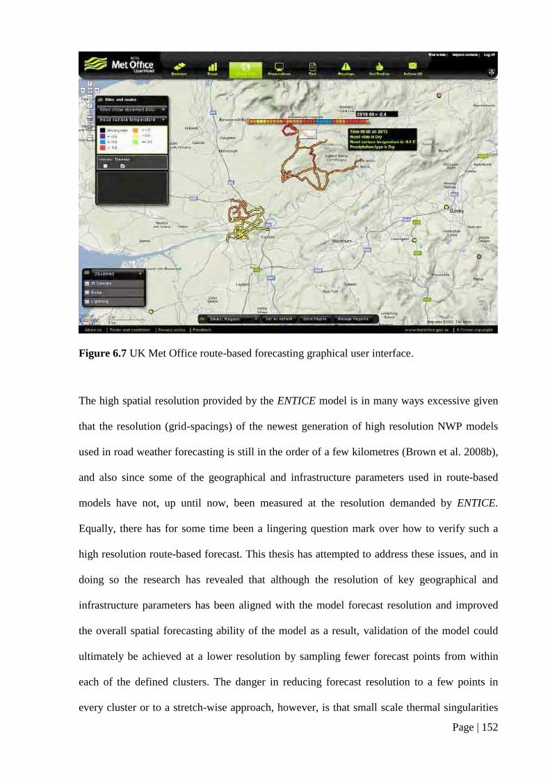
Page | 152
Figure 6.7 UK Met Office route-based forecasting graphical user interface.
The high spatial resolution provided by the ENTICE model is in many ways excessive given
that the resolution (grid-spacings) of the newest generation of high resolution NWP models
used in road weather forecasting is still in the order of a few kilometres (Brown et al. 2008b),
and also since some of the geographical and infrastructure parameters used in route-based
models have not, up until now, been measured at the resolution demanded by ENTICE.
Equally, there has for some time been a lingering question mark over how to verify such a
high resolution route-based forecast. This thesis has attempted to address these issues, and in
doing so the research has revealed that although the resolution of key geographical and
infrastructure parameters has been aligned with the model forecast resolution and improved
the overall spatial forecasting ability of the model as a result, validation of the model could
ultimately be achieved at a lower resolution by sampling fewer forecast points from within
each of the defined clusters. The danger in reducing forecast resolution to a few points in
every cluster or to a stretch-wise approach, however, is that small scale thermal singularities

Page | 153
such as katabatic frost hollows and minor bridge decks could potentially be omitted from
forecasts. Since the highway engineer has a duty of care to protect the motorist, it is essential
that these small scale variations are accounted for in road weather models, leading some to
suggest that ‘worst case scenario’ pessimistic forecasts may be a sensible approach for future
route-based forecasts (Chapman & Thornes 2008). However, the integration of thermal
mapping with a stretch-wise forecasting approach should help to identify such ‘cold spots’
around a road network, which could then be treated separately within the model. In the future
it is anticipated that many of these thermal features will be identified using downscaling
techniques on high resolution NWP models to obtain high resolution meteorological data
along small stretches of a route (Brown et al. 2008a; Brown et al. 2008b). Combine this with a
mobile infrared sensor such as IRIS positioned within each stretch-wise segment (or a cluster
of road stretches should they be further optimised), and full spatial validation of the route-
based forecast would be achievable without any need for thermal mapping surveys.
With the current advancements in shading and sky view estimation using a fully GIS-based
approach (Gal et al. 2007; Brown et al. 2008a), route-based forecasting is rapidly moving
towards a complete desktop surveying solution. However, local authorities are often not the
most flexible of organisations, and the safety of the public must always remain the top priority
even during the present challenging economic climate, so until these new desktop surveying
technologies have been thoroughly tested and proven to bring financial savings without
compromising safety, mobile surveying techniques will continue to be used in route-based
forecasting.

Page | 154
Figure 6.8 Schematic of the proposed next generation route-based forecasting system.
Figure 6.8 shows the synergy of the individual components discussed in this thesis in
providing the next generation of route-based road weather forecasts. Forecast providers are
likely to use high resolution NWP models with grid spacings of a few kilometres or less
which will be downscaled using a variety of new modelling techniques such as high
resolution valley parameterisation and lapse rate height based corrections (Brown et al.
2008a). These will allow more accurate prediction of topographic effects such as cold air
pooling and fog formation in valleys and enable better prediction of showers and convective
storms, and increased vertical resolution will improve the prediction of thin stratocumulus
clouds which in turn should lead to better near-surface temperature predictions (Brown et al.
2008b). Hence, downscaling techniques will create a high resolution meteorological dataset
for each individual stretch-wise segment of a route (typically 1 km in length), which will be
used to drive a surface energy balance model to predict RST and road state using a stretch-

Page | 155
wise approach. The spatial aspect of the route-based forecast is likely to be fully derived from
GIS-based desktop surveying techniques, with the addition of GPR subsurface data obtained
from local authority managed GPR databases. Satellite tracking of vehicle locations could
provide real-time traffic density data which forecast providers would be able to call upon in
order to more accurately parameterise the effects of traffic on the spatial variation of RST
around routes. Finally, strategic placing of a number of remote infrared RST sensors based on
the grouping of similar stretch-wise segments of roads using clustering techniques would
enable validation of the route-based forecast at a vastly improved spatial and temporal
resolution, eliminating the need for thermal mapping surveys.
Whilst numerous energy balance models are in existence, there has been a recent trend
towards the use of the METRo model which is now used throughout North America and is
becoming increasingly prevalent around Europe. The embedding of a route-based METRo
model into the MDSS framework (Chapter 1) would in many ways be the ideal solution in the
wider research context, given the popularity and widespread use of the METRo model which
has resulted in an abundance of knowledge and resources available to further test and develop
the model. Indeed, it is hoped that the findings of this research will provide the foundations
from which to start the development of a high resolution spatial component for the METRo
model.
In summary, the entire methodology of route-based forecasting is gradually changing as new
technologies emerge, and the transition towards a complete desktop surveying solution has
begun. Whilst the ENTICE model has been used as a case study, this model is no longer in
wide-scale commercial use, and the findings of this research will be of most benefit to the
development of a spatial component in the METRo model, which it is envisaged will become
the standard surface energy balance model for road weather forecasting over the next 10
years. The synergy of the various components shown in Figure 6.8 would need to be fully
tested before being phased in, as safety is of paramount importance in road weather

Page | 156
forecasting. Hence, the days of mobile surveying are not over just yet, but with further time
and effort the next generation of route-based road weather forecasts should soon emerge.
CHAPTER SIX SUMMARY
A number of refinements to the new re-parameterised road construction and surface
roughness measurement techniques have been discussed which it is suggested could further
improve the overall spatial forecasting ability of the ENTICE route-based forecast model. An
evaluation of the current technology available for parameterising traffic in route-based
forecast models has indicated that a satellite-based system perhaps offers the greatest
potential for providing high resolution traffic density data, but further work is required before
such a system can be realised. Particular attention has been drawn to the spatial resolution of
route-based forecasts given the current limitations of NWP models at resolutions higher than
4 km. However, advancements in model downscaling techniques suggest that a resolution in
the order of 1 km, which equates to a stretch-wise forecasting approach, will provide an
appropriate balance between the spatial accuracy demands of winter maintenance operations
and the capabilities of NWP models in providing high resolution meteorological data for
individual stretches of road. The synergy of all these components is presented as a blueprint
for the future of route-based road weather forecasts.

Page | 157
7. CONCLUSIONS
When route-based forecasting was first introduced nearly a decade ago, it was in some ways
ahead of its time since some of the geographical and infrastructure parameters used to drive
the spatial component of a route-based model had never been measured at the spatial scale
demanded by a route-based forecast. Similarly, the increased spatial resolution provided by
route-based forecasts has resulted in validation techniques which for many years served as a
benchmark for road weather models suddenly becoming wholly inadequate tools for model
validation. This thesis has aimed to address these issues by developing the foundations for a
new validation strategy for route-based forecasts that enables validation at a much higher
spatial and temporal resolution than is currently possible, and by de-parameterising key
geographical and infrastructure parameters within the ENTICE model to the spatial scale
demanded by a route-based forecast. This has been achieved by fulfilling the following
objectives outlined in Chapter 1.
1. To critically review existing road weather validation techniques as tools for verifying
route-based road weather forecasts.
The increased resolution of route-based road weather forecasts requires validation at a whole
new spatial scale in order to fully account for the variations in geographical and road
infrastructure parameters which influence thermal variations around a route. A review of
existing validation techniques has shown that, due to the vast number of forecast points that
need to be validated, no single technique was capable of achieving validation at anywhere
near the full spatial and temporal resolution of a route-based forecast. Hence, this highlighted
the need for a new validation methodology which could be used to provide a rapid appraisal
of model performance. Due to the large quantity of data involved data reduction techniques
provided a suitable starting point.

Page | 158
2. From the outcome of (1), devise a new methodology to facilitate validation of the ENTICE
model at a spatial scale previously unseen with route-based forecasts.
This objective was the key milestone of this research. It was essential to develop a technique
that allowed validation at a much higher spatial and temporal resolution than current
methodologies allow. The proposed clustering technique has been shown to provide a more
representative measure of the model’s spatial forecasting ability by segregating the validation
of routes into what are essentially high resolution climate zones, within which the
geographical and road infrastructure parameters have a greater influence on RST than the
meteorological parameters. The technique has been proven to repeatedly capture the spatial
distribution of temperature around a salting route, and hence the physical relation between
measured RST and the geographical and road infrastructure parameters controlling the
clustering. The methodology proposed could equally be used to optimise and verify stretch-
wise route-based forecasts, and has the potential to vastly improve the spatial and temporal
validation of route-based forecasts when used in conjunction with low cost infrared RST
sensors or similar measurement systems. Indeed, it is recommended that a low cost infrared
sensor be installed within each defined ‘geo-cluster’ as a starting point for improving the
spatial and temporal validation of route-based forecasts.
3. Investigate new techniques to remove geographical and infrastructure parameterisations in
the ENTICE model, namely:
i. Road construction re-parameterisation through the use of Ground Penetrating Radar
technology.
By surveying the subsurface road construction around a route using GPR technology, variable
depth profiles have been created in the ENTICE model that have been shown to provide a
more realistic representation of the true subsurface road construction around a route than was
attainable with the original parameterisation proposed by Chapman et al. (2001b). The depths
of subsurface layer interfaces have been estimated from GPR trace data via an inflexion point

Page | 159
algorithm designed to identify significant inflexions in the electromagnetic waveform of a
GPR trace. Calculated depths are then used to estimate subsurface temperatures and the
surface heat flux at each forecast point around the route. An increase of almost 7% in the
overall Pm values was observed in a statistical analysis on ENTICE road construction
parameterisation, indicating a significant improvement in the spatial forecasting ability of the
ENTICE model as a result of the new re-parameterised road construction measurements. The
methodologies used in parameterising subsurface layer depths from GPR measurements could
be used for subsurface layer depth parameterisation in other surface energy balance models,
particularly the METRo model where it is hoped the findings of this research will encourage
the development of a spatial component within the existing METRo heat conduction module.
ii. Surface roughness (land use) re-parameterisation using airborne LIDAR data.
Turbulent heat transfer in the boundary layer close to the road surface is represented in
ENTICE using a theoretical roughness length parameter. Existing parameterisation of Z0 fails
to account for the effect of upstream surface elements on local Z0 values at each forecast point
and the influence of the prevailing wind direction on local turbulence. A methodology has
been proposed that uses high resolution LIDAR data coupled with spatial processing
techniques to calculate an effective roughness length at each forecast point in a route-based
forecast from the distribution of local Z0 estimations within the upwind fetch of each forecast
point. A statistical analysis comparing RST forecast values obtained using the existing Z0
parameterisation with values obtained using the new Z0eff
measurements has revealed a 6%
increase in the variability of RST accounted for by ENTICE with the new re-parameterised
Z0eff
measurements. The methodologies proposed compliment other current research relating
to geographical parameterisations in route-based models, most notably the on-going Danish
Height Model research to estimate shadowing effects on RST using high resolution LIDAR
data (Pedersen et al. 2010).

Page | 160
4. To use the validation strategy devised in (2) as a new methodology for testing whether the
changes to geographical and infrastructure parameterisation improve the overall spatial
forecasting performance of the ENTICE model.
Changes to road construction and surface roughness parameterisation in the ENTICE model
have led to refinement of the clustering solution for the study route, and the spatial forecasting
ability of the model has been proven to increase through an analysis of forecast statistics at
the cluster level. On extreme nights during winter when atmospheric conditions are most
stable and RST is most likely to fall below zero, the refined clustering solution has been
shown, via CSC analysis, to better capture the physical relationship between RST and the
geographical and infrastructure parameters around the study route. Cluster level statistics
reveal poor model performance in city centre locations, believed to be linked to the
inadequate parameterisation of traffic in the ENTICE model, for which recommendations are
made in Chapter 6.
5. Make recommendations for the future of route-based forecasting.
The entire methodology of route-based forecasting is starting to change as new technologies
emerge, and with further time and effort these technologies will be utilised to their full
capabilities, enabling the next generation of route-based forecasts proposed in the blueprint in
Figure 6.8 to be realised. The spatial resolution of route-based forecasts is likely to be dictated
by the capabilities of high resolution NWP models over the coming years, and there is
sufficient evidence to suggest that geographical surveying techniques, whether mobile or
desktop based, will at some point in the future become surplus to requirements, with NWP
models themselves providing the geographical parameterisations required to drive the spatial
component of route-based forecast models. However, public safety must always remain the
top priority, so until these new technologies have been thoroughly tested and proven, mobile
and desktop surveying techniques will continue to be used in route-based forecasting.

Page | 161
To conclude, the specific aims and objectives of this thesis have been fulfilled. The findings
of this research should give winter maintenance engineers further confidence in route-based
forecasting, with a validation technique now in place which not only provides a better
representation of a models spatial forecasting ability, but also enables identification of those
areas within a route where model performance is not as accurate and where extra caution
should be exercised when making treatment decisions. Such locations are ideal sites for the
new generation of low cost infrared sensors now readily available, and such information will
be vital in helping local authorities progress towards selective salting strategies, where the
greatest financial savings in road weather forecasting will ultimately be found.

Page | 162
REFERENCES
Al-Qadi, I. & Lahouar, S., 2005. Measuring layer thickness with GPR - Theory to practice.
Construction and Building Materials, 19, 763-772.
American Society of Civil Engineers (ASCE)., 1996. Hydrology Handbook Second Edition.
ASCE Manuals and Reports on Engineering Practice No. 28, Washington, USA.
Astbury, A., 1996. Use of a high resolution mesoscale model to prepare site specific road
temperature. In Proceedings of the 8th International Road Weather Conference.
SIRWEC. Birmingham, pp. 122-128.
Arya, S., 1988. Introduction to micrometeorology, London: Academic Press.
Baik, J. & Kim, J., 1999. A numerical study of flow and pollutant dispersion characteristics in
urban street canyons. Journal of Applied Meteorology, 38, 1576-1589.
Bergendahl, S., 1998. A study of surface temperature variations with the use of IR-technique.
In Earth Sciences Centre: B143. Univeristy of Göteborg.
Best, M., 2005. Representing urban areas within operational numerical weather prediction
models. Boundary-Layer Meteorology, 114, 91-109.
Bogren, J. & Gustavsson, T., 1991. Nocturnal air and road surface temperature variations in
complex terrain. International Journal of Climatology, 11, 443-455.
Bogren, J., Gustavsson, T., Karlsson, M. & Postgård, U., 2000. The impact of screening on
road surface temperature. Meteorological Applications, 7, 97-104.
Bogren, J., Gustavsson, T. & Lindqvist, S., 1992. A description of a local climatological
model used to predict temperature variations along stretches of road. Meteorological
Magazine, 121, 157-164.
Bogren, J., Gustavsson, T. & Postgård, U., 2000. Temperature differences in relation to
weather parameters. International Journal of Climatology, 20, 151-170.
Page | 163
Bottema, M., 1997. Urban roughness modelling in relation to pollutant dispersion.
Atmospheric Environment, 31, 3059-3075.
Brown, A., Jackson, S., Murkin, P., Sheridan, P., Skea, A., Smith, S., Veal, A. & Vosper, S.,
2008a. New techniques for route-based forecasting. In Proceedings of the 14th
Standing International Road Weather Conference. SIRWEC. Prague, Czech Republic,
ID17.
Brown, A., Jackson, S., Murkin, P., Skea, A., Smith, S. & Veal, A., 2008b. Weather
prediction for the road industry. In Proceedings of the 14th Standing International
Road Weather Conference. SIRWEC. Prague, Czech Republic, ID16.
Businger, J.A., 1986. Evaluation of the accuracy with which dry deposition can be measured
with current micrometeorological techniques. Journal of Climate and Applied
Meteorology, 25, 1100-1124.
Chapman, L., 2002. A Blueprint for 21st Century Road Ice Prediction. Birmingham:
University of Birmingham.
Chapman, L. & Thornes, J.E., 2004. Real-time sky-view factor calculation and
approximation. Journal of Atmospheric and Oceanic Technology, 21, 730-741.
Chapman, L. & Thornes, J.E., 2005. The influence of traffic on road surface temperatures:
implications for thermal mapping studies. Meteorological Applications, 12, 371-380.
Chapman, L. & Thornes, J.E., 2006. A geomatics-based road surface temperature prediction
model. Science of the Total Environment, 360, 68-80.
Chapman, L. & Thornes, J.E., 2008. Small-scale road surface temperature and condition
variations across a road profile. In Proceedings of the 14th Standing International
Road Weather Conference. SIRWEC. Prague, Czech Republic.
Chapman, L., Thornes, J.E. & Bradley, A., 2001a. Modelling of road surface temperature
from a geographical parameter database. Part 1: Statistical. Meteorological
Applications, 8, 409-419.

Page | 164
Chapman, L., Thornes, J.E. & Bradley, A., 2001b. Modelling of road surface temperature
from a geographical parameter database. Part 2: Numerical. Meteorological
Applications, 8, 421-436.
Chapman, L., Thornes, J.E., Muller, J.P. & McMuldroch, S., 2007. Potential applications of
thermal fisheye imagery in urban environments. IEEE Geoscience and Remote
Sensing Letters, 4(1), 56-59.
Christen, A. & Vogt, R., 2004. Energy and radiation balance of a central European city.
International Journal of Climatology, 24, 1394-1421.
Clark, W. & Hosking, P., 1986. Statistical methods for geographers, Chichester: Wiley.
Cleugh, H. & Oke, T., 1986. Suburban-rural energy balance comparisons in summer for
Vancouver, B.C. Boundary-Layer Meteorology, 36(4), 351-369.
Cornford, D. & Thornes, J., 1996. A comparison between spatial winter indices and
expenditure on winter road maintenance in Scotland. International Journal of
Climatology, 16, 339-357.
Crevier, L. & Delage, Y., 2001. METRo: A new model for road-condition forecasting in
Canada. Journal of Applied Meteorology, 40, 2026-2037.
Davenport, A.G., 1960. Rationale for determining design wind velocities. Journal of
Structural Division, American Society of Civil Engineers, 86, 39-68.
Demiryurek, U., Pan, B., Banaei-Kashani, F. & Shahabi, C., 2009. Towards the modelling of
traffic data on road networks. In 2nd International Workshop on Computational
Transportation Science. IWCTS 2009 Workshop Report. Seattle, Washington.
Department of Transport, 1984. Winter maintenance of motorways and trunk roads: statement
of service and code of practice.
Department for Transport, 2004. Feasibility study of road pricing in the UK - A report to the
Secretary of State, Department for Transport.

Page | 165
Drobot, S., Chapman, M., Schuler, E., Wiener, G., Mahoney, W.P., Pisano, P.A. &
McKeever, B., 2010. Overview of the vehicle data translator. In Proceedings of the
15th Standing International Road Weather Conference. SIRWEC. Québec City,
Canada.
Dytham, C., 1999. Choosing and using statistics: A biologist's guide, Malden, MA: Blackwell
Science.
Edwards, S., Lavagno, L., Lee, E.A. & Sangiovanni-Vincentelli, A., 2002. Design of
Embedded Systems: Formal Models, Validation and Synthesis. In De Micheli, G.,
Ernst, R. & Wolf, W., (eds). Readings in hardware/software co-design. San Francisco,
Academic Press.
Gal, T., Rzepa, M., Gromek, B. & Unger, J., 2007. Comparison between sky view factor
values computed by two different methods in an urban environment. Acta
Climatologica et Chorologica, (40-41), 17-26.
Gal, T., Lindberg, F. & Unger, J., 2009. Computing continuous sky view factors using 3D
urban raster and vector databases: comparison and application to urban climate.
Theoretical and Applied Climatology, 95, 111-123.
Garratt, J., 1992. The atmospheric boundary layer, Cambridge: Cambridge University Press.
Grimmond, C.S.B., 1992. Suburban energy balance, Vancouver. International Journal of
Climatology, 12(5), 481-497.
Grimmond, C.S.B. & Oke, T.R., 1995. Comparison of heat fluxes from summertime
observations in the suburbs of four North American cities. Journal of Applied
Meteorology, 34, 873-889.
Grimmond, C.S.B. & Oke, T.R., 1999a. Heat storage in urban areas: local-scale observations
and evaluation of a simple model. Journal of Applied Meteorology, 38, 922-940.
Grimmond, C.S.B. & Oke, T.R., 1999b. Aerodynamic properties of urban areas derived from
analysis of surface form. Journal of Applied Meteorology, 38, 1262-1292.

Page | 166
Grimmond, C.S.B., Salmond, J.A., Oke, T.R., Offerle, B. & Lemonsu, A., 2004. Flux and
turbulence measurements at a dense urban site in Marseille: heat, mass (water, carbon
dioxide) and momentum. Journal of Geophysical Research, Atmospheres, 109, 1-19.
Grimmond, C.S.B., Potter, S.K., Zutter, H.N. & Souch, C., 2001. Rapid methods to estimate
sky-view factors applied to urban areas. International Journal of Climatology, 21,
903-913.
Gustavsson, T., 1999. Thermal mapping - a technique for road climatological studies.
Meteorological Applications, 6, 385-394.
Gustavsson, T. & Bogren, J., 1993. Evaluation of a local climatological model - test carried
out in the county of Halland, Sweden. Meteorological Magazine, 122, 257-266.
Gustavsson, T., Bogren, J. & Green, C., 2001. Road climate in cities: A study of the
Stockholm area, south-east Sweden. Meteorological Applications, 8, 481-489.
Gustavsson, T., Karlsson, M., Bogren, J. & Lindqvist, S., 1998. Development of temperature
patterns during clear nights. Journal of Applied Meteorology, 559-571.
Handa, H., Chapman, L. & Yao, X., 2007. Robust salting route optimization using
evolutionary algorithms. Studies in Computational Intelligence, 51, 497-517.
Hanna, S. & Chang, J., 1992. Boundary layer parameterisations for applied dispersion
modelling over urban areas. Boundary Layer Meteorology, 58, 229-259.
Harman, I., Best, M. & Belcher, S., 2004. Radiative exchange in an urban street canyon.
Boundary-Layer Meteorology, 110, 301-316.
Hartigan, J., 1975. Clustering Algorithms, New York: Wiley.
Heilman, J.L., Brittin, C.L. & Neale, C.M.U., 1989. Fetch requirements for bowen ratio
measurements of latent and sensible heat fluxes. Agricultural and Forest Meteorology,
44, 262-273.
Horst, T.W., 1999. The footprint for estimation of atmosphere-surface exchange fluxes by
profile techniques. Boundary-Layer Meteorology, 90, 171-188.

Page | 167
Horst, T.W. & Weil, J.C., 1994. How far is far enough? The fetch requirements for
micrometeorological measurement of surface fluxes. Journal of Atmospheric and
Oceanic Technology, 11, 1018-1025.
Kim, J. & Baik, J., 2001. Urban street-canyon flows with bottom heating. Atmospheric
Environment, 35, 3395-3404.
Kondo, A., Ueno, M., Kaga, A. & Yamaguchi, K., 2001. The influence of urban canopy
configuration on urban albedo. Boundary-Layer Meteorology, 100, 225-242.
Kristiansen, K., Loisy, C. & Bosch, W., 2003. Road traffic monitoring by satellite. ESA
Bulletin, 52-57.
Lagourade, J., Kerr, Y. & Brunet, Y., 1995. An experimental study of angular effects on
surface temperature for various plant canopies and bare soils. Agricultural and Forest
Meteorology, 77, 167-190.
Lahouar, S. & Al-Qadi, I., 2008. Automatic detection of multiple pavement layers from GPR
data. NDT & E International, 41(2), 69-81.
Linden, S. & Drobot, S., 2010. The evolution of METRo in a roadway DSS. In Proceedings
of the 15th International Road Weather Conference. SIRWEC. Québec City, Canada.
Liou, K., 2002. An Introduction to Atmospheric Radiation Second Edition., London:
Academic Press.
Mahoney, W., Bernstein, B., Wolff, J., Linden, S., Myres, W.L., Hallowell, R.G., Cowie, J.,
Stern, A.D., Koenig, G., Phetteplace, G., Schultz, P., Pisano, P.A. & Burkheimer, D.,
2005. FHWA's Maintenance Decision Support System Project: Results and
Recommendations. Transportation Research Board: Journal of the Transportation
Research Board, 1911, 133-142.
Maisey, P., Hopwood, W. & Pearman, I., 2000. Impact of high resolution site specific
modelling on road surface temperature forecasts. In Proceedings of the 10th
International Road Weather Conference. SIRWEC. Davos, Switzerland, pp. 41-45.

Page | 168
Masson, V., 2000. A physically-based scheme for the urban energy balance in atmospheric
models. Boundary-Layer Meteorology, 94, 357-397.
McClure, D. & Graham, A., 2006. eCall - The Case for Deployment in the UK, Department
for Transport.
Moore, D., 1975. The friction of pneumatic tyres, Oxford: Elsevier Scientific.
Morey, R., 1998. Ground Penetrating Radar for evaluating subsurface conditions for
transportation facilities. National Cooperative Highway Research Program Synthesis
255.
Mylne, K.R., 1999. The use of forecast value calculations for optimising decision making
using probability forecasts. In Proceedings of the 17th Conference on Weather
Analysis and Forecasting. Denver, Colorado, USA.
Myrup, L., 1969. A numerical model of the urban heat island. Journal of Applied
Meteorology, 8, 908-919.
Neal, A., 2004. Ground-penetrating radar and its use in sedimentology: principles, problems
and progress. Earth-Science Reviews, 66, 261-330.
Nunez, M. & Oke, T., 1977. The energy balance of an urban canopy. Journal of Applied
Meteorology, 16, 11-19.
Offerle, B., Grimmond, C.S.B., Fortuniak, K., Klysik, K. & Oke, T.R., 2006. Temporal
variations in heat fluxes over a central European city centre. Theoretical and Applied
Climatology, 84, 103-116.
Offerle, B., Eliasson, I., Grimmond, C.S.B. & Holmer, B., 2007. Surface heating in relation to
air temperature, wind and turbulence in an urban street canyon. Boundary-Layer
Meteorology, 122, 273-292.
Oke, T.R., 1992. Boundary Layer Climates Second Edition., London: Routledge.

Page | 169
Oke, T.R., Sproken-Smith, R.A., Jáuregui, E. & Grimmond, C.S.B., 1999. The energy balance
of central Mexico City during the dry season. Atmospheric Environment, 33, 3919-
3930.
Ostafe, M., 2009. eCall Toolbox. eSafetySupport.org. Available at: http://www.esafety
support.org/en/ecall_toolbox/ [Accessed April 13, 2010].
Outcalt, S., 1971. A numerical surface climate simulator. Geographical Analysis, 3, 379-393.
Outcalt, S., 1972. The development and application of a simple digital surface-climate
simulator. Journal of Applied Meteorology, 11, 629-636.
Owen, S.M., MacKenzie, A.R., Bunce, R.G.H., Stewart, H.E., Donovan, R.G., Stark, G. &
Hewitt, C.N., 2006. Urban land classification and its uncertainties using principal
component and cluster analyses: A case study for the UK West Midlands. Landscape
and Urban Planning, 78, 311-321.
Parmenter, B. & Thornes, J., 1986. The use of a computer model to predict the formation of
ice on road surfaces. Transport and Road Research Laboratory Research Report, 71,
1-19.
Pedersen, T.S., Petersen, C., Sattler, K. & Mahura, A., 2010. Physiographic data for road
stretch forecasting. In Proceedings of the 15th Standing International Road Weather
Conference. SIRWEC. Québec City, Canada.
Petty, K. & Mahoney, W., 2008. The U.S. Federal Highway Administration Winter Road
Maintenance Decision Support System (MDSS): Recent Enhancements and
Refinements. In Proceedings of the 14th Standing International Road Weather
Conference. Prague, Czech Republic.
Preisendorfer, R., 1988. Principal components analysis in meteorology and oceanography.,
New York: Elsevier.

Page | 170
Prusa, J.M., Segal, M., Temeyer, B.R., Gallus, W.A. & Takle, E.S., 2002. Conceptual and
scaling evaluation of vehicle traffic thermal effects on snow/ice covered roads.
Journal of Applied Meteorology, 41, 1225-1240.
Quarmby, D., Smith, B. & Green, C., 2010. The resilience of England's transport system in
winter. An independent review - interim report, London: Department for Transport.
Rayer, P., 1987. The Meteorological Office forecast road surface temperature model.
Meteorological Magazine, 116, 180-191.
Salmond, J.A., Oke, T.R., Grimmond, C.S.B., Roberts, S. & Offerle, B., 2005. Venting of
heat and carbon dioxide from urban canyons at night. Journal of Applied Meteorology,
44, 1180-1194.
Schaudt, K.J., 1998. A new method for estimating roughness parameters and evaluating the
quality of observations. Journal of Applied Meteorology, 37, 470-476.
Schmid, H., 1994. Source areas for scalars and scalar fluxes. Boundary-Layer Meteorology,
67, 293-318.
Schultz, P., 2005. An ensemble of WRF and MM5 configurations for winter weather
forecasting. In Joint WRF/MM5 Users Workshop. Boulder, Colorado, p. 4.
Scott, J., 1986. Incorporation of angular emissivity effects in long wave infrared image
models. SPIE, 687, 44-53.
Seber, G., 2004. Multivariate observations., Chichester: Wiley.
Shao, J., 1990. A winter road surface temperature model with comparison to others.
Unpublished PhD thesis. UK: University of Birmingham.
Shao, J., 1998. Improving nowcasts of road surface temperature by a backpropagation neural
network. Weather and Forecasting, 13, 164-171.
Shao, J. & Lister, P., 1995. The prediction of road surface state and simulation of the shading
effect. Boundary-Layer Meteorology, 73(4), 411-419.

Page | 171
Shao, J. & Lister, P., 1996. An automated nowcasting model of road surface temperature and
State for winter road maintenance. Journal of Applied Meteorology, 35, 1352-1361.
Shao, J., Lister, P.J., Hart, G.D. & Pearson, H.B., 1996. Thermal mapping: reliability and
repeatability. In Proceedings of the 8th International Road Weather Conference.
SIRWEC. Birmingham, pp. 235-242.
Shao, J., Swanson, J.C., Patterson, R., Lister, P.J. & McDonald, A.N., 1997. Variation of
winter road surface temperature due to topography and application of thermal
mapping. Meteorological Applications, 4(2), 131-137.
Sheskin, D., 2007. Handbook of Parametric and Nonparametric Statistical Procedures Fourth
Edition., London: Chapman & Hall//CRC.
Sini, J., Anquetin, S. & Mestayer, P., 1996. Pollutant dispersion and thermal effects in urban
street canyons. Atmospheric Environment, 30, 2659-2677.
Smith, C., Lindley, S. & Levermore, G., 2009. Estimating spatial and temporal patterns of
urban anthropogenic heat fluxes for UK cities: the case of Manchester. Theoretical
and Applied Climatology, 98, 19-35.
Sneath, P. & Sokal, R., 1973. Numerical taxonomy - the principles and practice of numerical
classification., San Francisco: W.H.Freeman.
Stephenson, D.B., 2000. Use of the 'odds ratio' for diagnosing forecast skill. Weather and
Forecasting, 15, 221-232.
Sugrue, G., 1983. Infrared thermometry - advantages and disadvantages. In Atmosphere-Road
Surface Interaction Group Working Paper 7.
Tieleman, H.W., 2003. Roughness estimation for wind-load simulation experiments. Journal
of Wind Engineering and Industrial Aerodynamics, 91, 1163-1173.
Thompson, N., 1988. The Meteorological Office road surface temperature prediction model.
In Proceedings of the 4th International Road Weather Conference. Florence, Italy.

Page | 172
Thornes, J.E., 1984. The prediction of ice formation on motorways in Britain. London:
University of London.
Thornes, J.E., 1985. The prediction of ice formation on roads. Journal of the Institution of
Highways and Transportation, 32, 3-12.
Thornes, J.E., 1991. Thermal mapping and road-weather information systems for highway
engineers. In Highway Meteorology. London: E & FN Spon, pp. 39-67.
Thornes, J.E., 1994. Salt of the Earth. The Surveyor. 8 December, 16-18.
Thornes, J.E., 1995. A comparative real-time trial between the Met Office and Oceanroutes to
predict road surface temperatures. Meteorological Applications, 2, 113-119.
Thornes, J.E., 1996. The cost benefit of winter road maintenance in the United Kingdom. In
Proceedings of the 8th International Road Weather Commission. SIRWEC.
Birmingham, pp. 1-10.
Thornes, J.E. & Shao, J., 1992. Objective method for improving the operational performance
of a road ice prediction model using interpolated mesoscale output and a template for
correcting systematic error. Meteorological Magazine, 121, 197-204.
Thornes, J.E. & Proctor, E.A.J., 1999. Persisting with persistence: the verification of Radio 4
weather forecasts. Weather, 54, 311-321.
Thornes, J.E. & Stephenson, D.B., 2001. How to judge the quality and value of weather
forecast products. Meteorological Applications, 8, 307-314.
Vihma, T. & Savijärvi, H., 1991. On the effective roughness length for heterogeneous terrain.
Quarterly Journal of the Royal Meteorological Society, 117, 399-407.
White, S., 2007. The route treatment. Surveyor Magazine, 12-14.
Wieringa, J., 1992. Updating the Davenport roughness classification. Journal of Wind
Engineering and Industrial Aerodynamics, 41, 357-368.
Wieringa, J., 1993. Representative roughness parameters for homogeneous terrain. Boundary
Layer Meteorology, 63, 323-363.

Page | 173
Wieringa, J., Davenport, A.G., Grimmond, C.S.B. & Oke, T.R., 2001. New revision of
Davenport roughness classification. In Proceedings of the 3rd European & African
Conference on Wind Engineering. Eindoven, Netherlands, p. 8.
Wimsatt, A. et al., 1998. Use of ground penetrating radar data in pavement rehabilitation
strategy selection and pavement condition assessment. In Proceedings of SPIE Volume
3400. Structural Materials Technology III: An NDT Conference. San Antonio, TX,
USA, pp. 372-383.
Yoshida, A., Tominaga, K. & Watatani, S., 1991. Field measurements on energy balance of
an urban canyon in the summer season. Energy and Buildings, 15, 417-423.
WEBSITE ADDRESSES CITED IN TEXT
http://www.safecote.com/
http://meteogroup.co.uk/
http://landmap.ac.uk/
http://badc.nerc.ac.uk/home/index.html/
http://www.bluesky-world.com/
http://gna.org/projects/metro/

APPENDIX 1
MATLAB HIERARCHICAL CLUSTER PROGRAM
%RWIS Cluster Program Optional Settings % % Optional distance algorithms: % % 'euclidean' - Euclidean distance % 'seuclidean' - Standardized Euclidean distance. Each coordinate in the
sum of squares is inverse weighted by the sample variance of that %coordinate % 'cityblock' - City Block metric % 'minkowski' - Minkowski metric % 'cosine' - One minus the cosine of the included angle between points
(treated as vectors) % 'correlation' - One minus the sample correlation between points (treated
as sequences of values). % 'spearman' - One minus the sample Spearman's rank correlation between
observations, % treated as sequences of values % % Optional linkage algorthims: % % 'single' - Shortest distance % 'complete' - Furthest distance % 'average' - Unweighted average distance (UPGMA) (also known as group
average) % 'weighted' - Weighted average distance (WPGMA) % 'centroid' - Centroid distance (UPGMC) % 'median' - Weighted center of mass distance (WPGMC) % 'ward' - Inner squared distance (minimum variance algorithm)
clc; input ('RWIS Cluster Program. Press Enter to start: '); filename = input ('Enter survey filename within single quotes, e.g.
''Test'': '); file_name = input ('Enter output filename within single quotes, e.g.
''Cluster_PhDleices'': '); %rst_data = input ('Enter filename containing RST data, e.g.
''Test_20080217.xls'': '); disp('Importing Excel survey file') [data, headings, raw] = xlsread(filename,'A:P'); D = data(:,6:12); %select data columns required for analysis X = zscore(D); %normalize the data Y1 = pdist(X,'euclidean'); %calculate distance between all object pairs -
various methods of distance methods can be specified - euclidean is default Z1 = linkage(Y1,'average'); %use linkage function to determine how objects
in the data set should be grouped into clusters linkage method can be
specified - single is default dendrogram(Z1); %plot hierarchical binary cluster tree information as a
graph hold on; xlabel('Cluster'); ylabel('Cluster link height'); c1 = cophenet(Z1,Y1); %calculate cophenetic correlation coefficient -
closer to 1 this value is, the more accurately the clustering solution
reflects data %rst = xlsread(rst_data,'Join_Output','CM2:CN2146');

title = {'ICOEFF' 'CLUSTER' 'CLUSTER_STD' '' 'FORECAST_RST' 'ACTUAL_RST'
'ACTUAL_RST_STD' 'ERROR' 'MOD_ERROR' 'MOD_LOGIC' 'SQ_ERROR' 'BIAS'
'SD_of_BIAS' 'RMSE' '%FORECAST_WITHIN_1DEG_ACTUAL' 'RESID_FORECAST'
'RESID_ACTUAL' 'RESID_ERROR' 'MOD_RESID_ERROR' 'MOD_RESID_LOGIC'
'%RESID_FORECAST_WITHIN_1DEG_RESID_ACTUAL' 'STDEV_STABILITY'}; code1 = {'=standardize(V3,average(V$3:V$2263),stdev(V$3:V$2263))' '=U3-V3'
'=if(X3<0,X3*-1,X3)' '=if(Y3<=1,1,0)' '=X3^2'}; code2 = {'=average(X3:X2263)' '=stdev(X3:X2263)' '=average(AA3:AA2263)^0.5'
'=sum(Z3:Z2263)/2263*100'}; code3 = {'=U3-average(U$3:U$2263)' '=V3-average(V$3:V$2263)' '=AF3-AG3'
'=if(AH3<0,AH3*-1,AH3)' '=if(AI3<=1,1,0)'}; code4 = {'=sum(AJ3:AJ2263)/2263*100' '=stdev(V3:V2263)'};
for i = 10:2:12; str = num2str(i); str2 = ['Analysing data and organising into ' str ' clusters']; disp(' ') disp(str2) warning off MATLAB:xlswrite:AddSheet clust = cluster(Z1,'maxclust',i); clust_std = zscore(clust); xlswrite(file_name,headings,str,'A1'); xlswrite(file_name,title,str,'Q1'); xlswrite(file_name,clust,str,'R3'); xlswrite(file_name,clust_std,str,'S3'); %xlswrite(file_name,rst,str,'P3'); xlswrite(file_name,data,str,'A3'); xlswrite(file_name,c1,str,'Q3'); xlswrite(file_name,code1,str,'W3:AA2263'); xlswrite(file_name,code2,str,'AB3:AE3'); xlswrite(file_name,code3,str,'AF3:AJ2263'); xlswrite(file_name,code4,str,'AK3:AL3'); str3 = ['Clustering complete for ' str ' clusters']; disp(str3) end;
disp('Hierarchical Clustering Complete!)
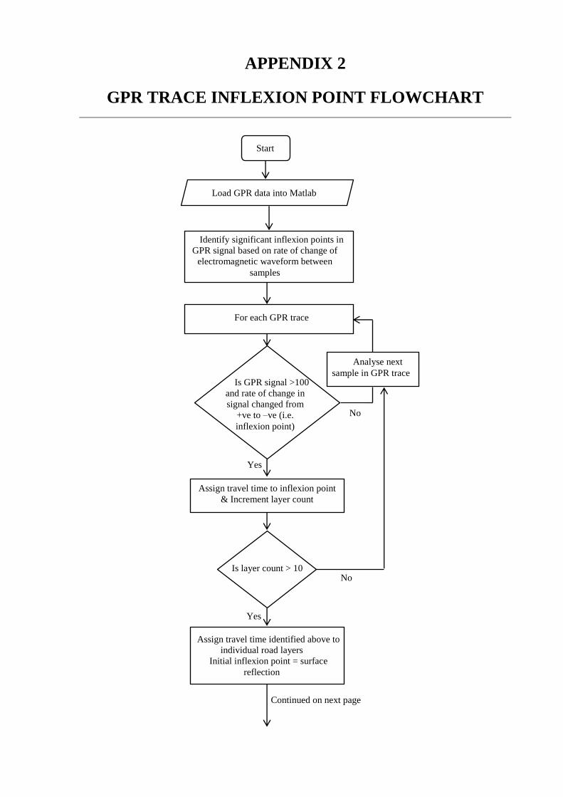
APPENDIX 2
GPR TRACE INFLEXION POINT FLOWCHART
Start
No
Analyse next
sample in GPR trace
Continued on next page
Load GPR data into Matlab
Identify significant inflexion points in
GPR signal based on rate of change of
electromagnetic waveform between
samples
Assign travel time to inflexion point
& Increment layer count
No
Yes
Is GPR signal >100
and rate of change in
signal changed from
+ve to –ve (i.e.
inflexion point)
Yes
Is layer count > 10
For each GPR trace
Assign travel time identified above to
individual road layers
Initial inflexion point = surface
reflection

Continued from previous page
Assign dielectric constant values to 5
road layers
Asphalt = 6, Concrete = 10, Soil = 25
For each forecast point
Yes Yes Yes Yes
No No No Is road type
= C road
Is road type
= B road
Is road type
= A road Is road type
= motorway
If road layer
< = 3
material = asphalt
Else
If road layer = 5
material = concrete
* 0.8 + soil * 0.2
Else
material = concrete
If road layer
< = 3 or = 5
material = asphalt
Else
Material = concrete
If road layer
< = 3
material = asphalt
Else
If road layer = 5
material = concrete
* 0.5 + soil * 0.5
Else
material = concrete
If road layer = 1
material = asphalt
Else
If road layer < 5
material = concrete
Else
If road layer = 5
material = soil
For each forecast point calculate
the depth of all 5 layers based on
Eq 3.1
Depth = ((travel time * 3E8) /
2*material^(1/2))
End

APPENDIX 3
IRIS DATALOGGER PROGRAM
''--------------------------------------------------------------------------------------------
----------------------------
'' Program......................: IRIS Road Weather Station
''--------------------------------------------------------------------------------------------
----------------------------
'' Copyright....................: Copyright (C) 2006-2008 Campbell Scientific Ltd. All Rights
Reserved.
''--------------------------------------------------------------------------------------------
----------------------------
'' Author(s)....................: David Hammond, Simon Massey, Andrew Sandford
'' Company......................: Campbell Scientific Ltd
''--------------------------------------------------------------------------------------------
----------------------------
'' Version......................: 1.10.15 RELEASE
'' Last Revised.................: 06/05/2010
''--------------------------------------------------------------------------------------------
----------------------------
'' Notes........................: v1.10.15 originally modified by David Hammond, further
modified to utilise the full
'' .............................: 10 minute median due to timing changes.
'' .............................: - also includes updated modem configuration routine (SRM)
'' .............................:
''--------------------------------------------------------------------------------------------
----------------------------
'' Required Operating System(s).: CR800.Std.06.07 (BETA - Contains the 15 second connection
timeout fix from this version)
''--------------------------------------------------------------------------------------------
----------------------------
SequentialMode
PreserveVariables
AngleDegrees
'Debug Mode Control.
Const DebugMode = True 'When true enables all debug information within the IRIS program
(Default is False).
'Event Logging Control.
Const EventLogging = True 'When true enables event logging capability (Default is True).
'These defaults are used when no settings exist and should reflect the
'coefficients produced for the IR100 Sensor
Const DefaultIR100SerialNumber = ""
Const Default_Coeff_A = 9.434170E-04
Const Default_Coeff_B = 2.198455E-04
Const Default_Coeff_C = 1.388907E-07
Const Default_Coeff_X = 1.503168E-05
Const Default_Coeff_Y = 3.421465E-01
Const Default_Coeff_Z = -1.638007E-01
'This is the default Sky View Factor.
Const Default_SVF = 0.9
'Version Information
#If DebugMode Then
Const IRISProgVer = "IRIS.CR800.1.10.15.DIAG"
#Else
Const IRISProgVer = "IRIS.CR800.1.10.15"
#EndIf
'The name of the file that contains the IRIS settings.
Const IRISSettingsFilename = "USR:IRISCONFIG.INI"
'Comms Settings
Const ModemPort = ComME
Const CR = CHR(13)
'O2 Specific Configruation
Const PPPUsername="bypass"
Const PPPPassword="password"
'Modem set to numeric at 9600 baud (CSL default)
Const PPPdialresponse="21"

Const ModemNetwork = "mobile.O2.co.uk"
Const ModemConfig1 = CR & "AT+CGDCONT=1,""IP"",""" & ModemNetwork & """" & CR
Const ModemConfig2 = "AT+WIND=255" & CR
Const ModemConfig3 = "AT&W" & CR
Const DefaultTCPPort = 5794
Const DefaultPrimaryIPAddress = "81.110.79.59"
Const DefaultBackupIPAddress = "82.70.75.213"
Const MinimumBatteryThresholdForComms = 11 'Specified in Volts.
Const PPPTimeOut = 300 '60 'Maximum Time to Wait for a PPP connection in Seconds (back to 60)
Const PPPBlank = "0.0.0.0"
Const IPPortBlank = 0
Const IPTimeOut = 15 '120 'Maximum Time to Wait for an IP connection in Seconds.
Const COMMSTimeOut = 300 'The maximum time in seconds that the data connection will stay live.
Const ExtendedOnlineStartTime = 480 'Time in Minutes that extended online time starts. 480 =
8am.
Const ExtendedOnlineEndTime = 1080 'Time in Minutes that extended online time ends. 1080 =
6pm.
Const OneDayInMinutes = 1440 '24 Hours specified in minutes.
'Settings.
Const MaxNumberOfSettings = 8 'Maximum Number of Numeric Settings
Const MaxNumberOfStringSettings = 4 'Maximum Number of String Settings
Const STRINGSETTING_PrimaryIPAddress = 1
Const STRINGSETTING_BackupIPAddress = 2
Const STRINGSETTING_TCPPort = 3
Const STRINGSETTING_IR100SerialNumber = 4
Const SETTING_Emissivity = 1
Const SETTING_SVF = 2
Const SETTING_Coeff_A = 3
Const SETTING_Coeff_B = 4
Const SETTING_Coeff_C = 5
Const SETTING_Coeff_X = 6
Const SETTING_Coeff_Y = 7
Const SETTING_Coeff_Z = 8
'Film
Const Film = 0.79
'Surface Types
Const Asphalt = 0.956
Const Concrete = 0.966
Const Brick = 0.88
Const Ice = 0.97
Const Snow = 0.99
Const Ocean = 0.98
'On / Off
Const On = True
Const Off = False
'Traffic
Public Previous_TSurface
Public Traffic_Count1, Traffic_Count2, Traffic_Count3, Traffic_Count4
Public Traffic_Count11, Traffic_Count22, Traffic_Count33, Traffic_Count44
Public Difference_TSurface
'Controls Event Logging Capability.
#If EventLogging Then
'IRIS Event Logging Constants.
Const IRISEventLogMaximumSize = 20
Const IRISEventDescriptionMaximumLength = 32
Const IRISEventLogSize = 50 'The maximum size the event log can grow to.
Const IRISEventCode_Undefined = 0 'Indicates an event where no specific error code exists.
Const IRISEventCode_ProgramStarted = 1 'Indicates program started.
Const IRISEventCode_ProgramStopped = 2 'Indicates program stopped.
Const IRISEventCode_SettingsLoaded = 3 'Indicates IRIS settings file has been loaded from the
USR Drive
Const IRISEventCode_SettingsSaved = 4 'Indicates IRIS settings file has been saved to the USR
Drive
Const IRISEventCode_SettingsDefaulted = 5 'Indicates that default settings were stored.
Const IRISEventCode_CS215Error = 6 'Indicates an error with the CS215.
Const IRISEventCode_CommsStarting = 7 'Used to indicate that comms are beginning (DEBUG)
Const IRISEventCode_PPPStartFailed = 8 'Indicates PPP startup has failed.
Const IRISEventCode_PPPCloseFailed = 9 'Indicates PPP closing has failed.
Const IRISEventCode_IPConnectFailed = 10 'Indicates IP open with primary and backup has
failed.
Const IRISEventCode_ModemStartFailed = 11 'Indicates that the modem has failed to initialise.
Const IRISEventCode_BatteryTooLowForComms = 12 'Indicates that the battery has too little
power for comms to run.
'IRIS Event Logging Variables.
Dim IRISEventCode As Long 'Stores the event code to be sampled.
Dim IRISEventDescription As String * IRISEventDescriptionMaximumLength 'Stores an event
description to be sampled.
Dim IRISEventLog(IRISEventLogMaximumSize,2) As String * IRISEventDescriptionMaximumLength

Dim IRISEventLogCurrentPosition As Long
Dim SavingEventLog As Boolean
#EndIf
'Debuggable Variable Declarations (note dependent on debug mode)
#If DebugMode Then
Public IRISProgramVersion As String * 50 'Holds the current version of the program for
sampling
'Menu and Settings Control.
Public MENUStringSettings(MaxNumberOfStringSettings) As String * 20
Public StringSettings(MaxNumberOfStringSettings) As String * 20
Public MENUSettings(MaxNumberOfSettings) 'Stores the settings as modified through the menu.
Public Settings(MaxNumberOfSettings) 'Stores the settings currently being used by the program.
Public SettingsChanged As Boolean 'This flag will be set if the settings are changed in the
menus.
Public SettingsLoading As Boolean 'This flag is set if the settings are currently being
reloaded.
Public ReloadSettings As Boolean 'If this flag is set to true then the settings will be
reloaded at the top of the next minute.
'Working Variables.
Public PTemp, Batt_Volt, FirstRun As Boolean
Public CS215(2)
Public CosBeta_A, CosBeta_B, CosBeta_C, CosBeta_D
Public SVF, SVP, VP
Public Dew_Point, SkyTemp
Public Cal_Can, IRSensor_Resis, IRSensorCan_Temp, IRSensor_Volt, IRSensor_E, IRSensor_T4,
IRSensor_T, IRTemp, IRSensor_Volt_TC
Public TSurface, TFilm
Public IRSpreadIndex
'Communications Variables
Public OpenPPP As String * 30
Public ConnectDelay As Boolean
Public COMMSTimer 'Uses Timer 0
Public PPPAddress As String * 20
Public ModemStarted As Boolean 'This flag is set to true if the modem is started successfully.
Public IPPort As Long, CommsTCPPort As Long, SendResult, Scratch
Public ModemConfigured As Boolean
#Else
Dim IRISProgramVersion As String * 50 'Holds the current version of the program for sampling
'Menu and Settings Control.
Dim MENUStringSettings(MaxNumberOfStringSettings) As String * 20
Dim StringSettings(MaxNumberOfStringSettings) As String * 20
Dim MENUSettings(MaxNumberOfSettings) 'Stores the settings as modified through the menu.
Dim Settings(MaxNumberOfSettings) 'Stores the settings currently being used by the program.
Dim SettingsChanged As Boolean 'This flag will be set if the settings are changed in the
menus.
Dim SettingsLoading As Boolean 'This flag is set if the settings are currently being reloaded.
Public ReloadSettings As Boolean 'If this flag is set to true then the settings will be
reloaded at the top of the next minute.
'Working Variables.
Dim PTemp, Batt_Volt, FirstRun As Boolean
Dim CS215(2)
Dim CosBeta_A, CosBeta_B, CosBeta_C, CosBeta_D
Dim SVF, SVP, VP
Dim Dew_Point, SkyTemp
Dim Cal_Can, IRSensor_Resis, IRSensorCan_Temp, IRSensor_Volt, IRSensor_E, IRSensor_T4,
IRSensor_T, IRTemp, IRSensor_Volt_TC
Dim TSurface, TFilm
Dim IRSpreadIndex
'Communications Variables
Dim OpenPPP As String * 30
Dim ConnectDelay As Boolean
Dim COMMSTimer 'Uses Timer 0
Dim PPPAddress As String * 20
Dim ModemStarted As Boolean 'This flag is set to true if the modem is started successfully.
Dim IPPort As Long, CommsTCPPort As Long, SendResult, Scratch
Dim ModemConfigured As Boolean
#EndIf
'These public variables are used purely to provide live data during setup.
Public Live_RoadTemp, Live_AirTemp, Live_RH, Live_DewPoint, Live_PanelTemp, Live_Battery,
Live_BodyTemp
Public Live_SerialNumber As String * 10
'When true indicates that coefficients are available.
Public CoeffsAvailable As Boolean
'This variable is always public and ocntains a running status for GPRS comms.
Public CommsStep As String * 32
'When this flag is set the logger tmeperature will be used as a substitute for

'AirTemp and Dew_Point. This option is available to allow for data to be
'generated even if the CS215 should be unavailable.
Public UseLoggerTemperature As Boolean '(Default is False)
Alias CS215(1) = AirTemp
Alias CS215(2) = RH
'*****************************************************************************
'Table Name ..: IrisData
'Frequency....: 10 Minutes
'History......: Automatic
'Purpose......: The main data source for the IRIS Bureau
'*****************************************************************************
DataTable(IrisData,True,-1)
DataInterval(0,10,Min,10)
'Logger Stats.
Minimum(1,Batt_Volt,FP2,0,False) : FieldNames("Battery_Voltage")
Sample(1,PTemp,FP2) : FieldNames("Panel_Temp")
'IRIS Return Values.
Median(1,TSurface,120,FP2,False) : FieldNames("IRTemp")
Average(1,AirTemp,FP2,False) : FieldNames("Air_Temp")
Average(1,RH,FP2,False) : FieldNames("RH")
Average(1,Dew_Point,FP2,False) : FieldNames("Dew_Point")
'Status Flags
Sample(1,UseLoggerTemperature,Boolean) : FieldNames("UsingLoggerTemperature")
EndTable
'*****************************************************************************
'Table Name ..: Traffic
'Frequency....: 10 Minutes
'History......: Automatic
'Purpose......: Stores total traffic count information
'*****************************************************************************
DataTable(Traffic,True,-1)
DataInterval(0,10,Min,10)
Totalize(1,Traffic_Count1,FP2,False)
Totalize(1,Traffic_Count2,FP2,False)
Totalize(1,Traffic_Count3,FP2,False)
Totalize(1,Traffic_Count4,FP2,False)
Totalize(1,Traffic_Count11,FP2,False)
Totalize(1,Traffic_Count22,FP2,False)
Totalize(1,Traffic_Count33,FP2,False)
Totalize(1,Traffic_Count44,FP2,False)
EndTable
#If EventLogging Then
'*****************************************************************************
'Table Name ..: IRISEventLog
'Frequency....: as required, no fixed interval
'History......: as defined by IRISEventLogSize constant
'Purpose......: Stores IRIS Events for logging purposes,
'.............: records are added by calling the LogEvent procedure.
'*****************************************************************************
DataTable(IRISEventLog,True,IRISEventLogSize)
Sample(1,IRISEventCode,Long) : FieldNames("EventCode")
Sample(1,IRISEventDescription,String) : FieldNames("EventDescription")
EndTable
'This procedure takes an event code and and event description and stores them to the IRIS
Event Log.
Sub LogEvent(LogEvent_EventCode As Long, LogEvent_EventDescription As String *
IRISEventDescriptionMaximumLength)
'Transfer the event details ready for sampling later
If NOT SavingEventLog Then
If IRISEventLogCurrentPosition <= IRISEventLogMaximumSize Then
IRISEventLog(IRISEventLogCurrentPosition,1) = LogEvent_EventCode
IRISEventLog(IRISEventLogCurrentPosition,2) = LogEvent_EventDescription
IRISEventLogCurrentPosition = IRISEventLogCurrentPosition + 1
EndIf
EndIf
EndSub
'This procedure copies all the currently stored events to the table.
Dim SaveEventLogIndex As Long
Sub SaveEventLog
SavingEventLog = True
If IRISEventLogCurrentPosition > 1 Then
For SaveEventLogIndex = 1 To (IRISEventLogCurrentPosition - 1)
IRISEventCode = IRISEventLog(SaveEventLogIndex,1)
IRISEventDescription = IRISEventLog(SaveEventLogIndex,2)

'Store the event in the event log.
CallTable IRISEventLog
Next SaveEventLogIndex
EndIf
IRISEventLogCurrentPosition = 1
SavingEventLog = False
EndSub
#EndIf
Dim ConfigureModemSucceeded As Boolean
Sub ConfigureModem(ConfigureModemSuccess As Boolean)
ConfigureModemSucceeded = True
SW12(On)
Delay(1,10,Sec)
SerialOpen(ModemPort,9600,0,20000,1000)
If SerialOut(ModemPort,"ATV0" & CHR(13),"0",1,150) = 0 Then ConfigureModemSucceeded = False
If SerialOut(ModemPort,"ATE1" & CHR(13),"0",1,150) = 0 Then ConfigureModemSucceeded = False
If SerialOut(ModemPort,ModemConfig1,"0",1,150) = 0 Then ConfigureModemSucceeded = False
If SerialOut(ModemPort,ModemConfig2,"0",1,150) = 0 Then ConfigureModemSucceeded = False
If SerialOut(ModemPort,ModemConfig3,"0",1,150) = 0 Then ConfigureModemSucceeded = False
SerialClose(ModemPort)
SW12(Off)
ConfigureModemSuccess = ConfigureModemSucceeded
EndSub
'This procedure generates menus for changing settings.
Sub GenerateSettingsMenu
DisplayMenu("IRIS Main Menu",-1)
SubMenu("Live Values")
DisplayValue("Road Temp",Live_RoadTemp)
DisplayValue("Air Temp",Live_AirTemp)
DisplayValue("RH",Live_RH)
DisplayValue("Dew Point",Live_DewPoint)
DisplayValue("Panel Temp",Live_PanelTemp)
DisplayValue("Battery",Live_Battery)
EndSubMenu
SubMenu("Communications")
MenuItem("TCP Port",MENUStringSettings(STRINGSETTING_TCPPort))
MenuItem("IP Address",MENUStringSettings(STRINGSETTING_PrimaryIPAddress))
MenuItem("Backup IP",MENUStringSettings(STRINGSETTING_BackupIPAddress))
EndSubMenu
SubMenu("IR100 Settings")
MenuItem("Serial #",MENUStringSettings(STRINGSETTING_IR100SerialNumber))
MenuItem("Coeff A",MENUSettings(SETTING_Coeff_A))
MenuItem("Coeff B",MENUSettings(SETTING_Coeff_B))
MenuItem("Coeff C",MENUSettings(SETTING_Coeff_C))
MenuItem("Coeff X",MENUSettings(SETTING_Coeff_X))
MenuItem("Coeff Y",MENUSettings(SETTING_Coeff_Y))
MenuItem("Coeff Z",MENUSettings(SETTING_Coeff_Z))
EndSubMenu
SubMenu("Emissivity")
MenuItem("Surface",MENUSettings(SETTING_Emissivity))
MenuPick(Asphalt,Concrete,Brick,Ice,Snow,Ocean)'Pick list for Emissivity
EndSubMenu
SubMenu("Sky View Factor")
MenuItem("SVF Value",MENUSettings(SETTING_SVF))
EndSubMenu
EndMenu
EndSub
'This procedure saves the current menu settings to file and transfers them into actual
locations.
Dim SaveSettings_FileHandle As Long
Dim SaveSettings_OutputString As String * 400
Dim SaveSettings_Index As Long
Sub SaveSettings
SettingsChanged = False
SaveSettings_FileHandle = FileOpen(IRISSettingsFilename,"w",0)
If SaveSettings_FileHandle <> 0 Then
'Generate an output string from the current menu settings.
SaveSettings_OutputString = ""
'Numeric
For SaveSettings_Index = 1 To MaxNumberOfSettings
SaveSettings_OutputString = SaveSettings_OutputString & MENUSettings(SaveSettings_Index)
& ","
Next SaveSettings_Index
'Strings
For SaveSettings_Index = 1 To MaxNumberOfStringSettings

SaveSettings_OutputString = SaveSettings_OutputString &
MENUStringSettings(SaveSettings_Index) & ","
Next SaveSettings_Index
'Save new settings to file.
FileWrite(SaveSettings_FileHandle,SaveSettings_OutputString,0)
'Transfer new settings to actual locations.
'Numeric
For SaveSettings_Index = 1 To MaxNumberOfSettings
Settings(SaveSettings_Index) = MENUSettings(SaveSettings_Index)
Next SaveSettings_Index
'Strings
For SaveSettings_Index = 1 To MaxNumberOfStringSettings
StringSettings(SaveSettings_Index) = MENUStringSettings(SaveSettings_Index)
Next LoadSettings_Index
'Copy Values where necessary.
SVF = Settings(SETTING_SVF)
Live_SerialNumber = StringSettings(STRINGSETTING_IR100SerialNumber)
EndIf
FileClose(SaveSettings_FileHandle)
#If EventLogging Then
'Log a startup event and include version.
LogEvent(IRISEventCode_SettingsSaved,IRISSettingsFilename)
#EndIf
EndSub
'This procedure loads the settings from the settings file,
'if no file exists then it loads defaults and create a new settings file.
Dim LoadSettings_FileHandle As Long
Dim SettingsFileLine As String * 400
Dim SettingsStringResult(MaxNumberOfSettings + MaxNumberOfStringSettings) As String
Dim LoadSettings_Index As Long
Sub LoadSettings
SettingsLoading = True
ReloadSettings = False
LoadSettings_FileHandle = FileOpen(IRISSettingsFilename,"r",0)
If LoadSettings_FileHandle = 0 Then
'Unable to find or open the file, so default all values.
'Strings
MENUStringSettings(STRINGSETTING_PrimaryIPAddress) = DefaultPrimaryIPAddress
MENUStringSettings(STRINGSETTING_BackupIPAddress) = DefaultBackupIPAddress
MENUStringSettings(STRINGSETTING_TCPPort) = DefaultTCPPort
MENUStringSettings(STRINGSETTING_IR100SerialNumber) = DefaultIR100SerialNumber
'Numeric
MENUSettings(SETTING_Emissivity) = Asphalt
MENUSettings(SETTING_SVF) = Default_SVF
MENUSettings(SETTING_Coeff_A) = Default_Coeff_A
MENUSettings(SETTING_Coeff_B) = Default_Coeff_B
MENUSettings(SETTING_Coeff_C) = Default_Coeff_C
MENUSettings(SETTING_Coeff_X) = Default_Coeff_X
MENUSettings(SETTING_Coeff_Y) = Default_Coeff_Y
MENUSettings(SETTING_Coeff_Z) = Default_Coeff_Z
#If EventLogging Then
'Log a startup event and include version.
LogEvent(IRISEventCode_SettingsDefaulted,IRISSettingsFilename)
#EndIf
'Now store the values as they didn't exist.
SaveSettings
Else
'Load the settings from the file.
FileReadLine(LoadSettings_FileHandle,SettingsFileLine,200)
'Split the values up.
SplitStr(SettingsStringResult(),SettingsFileLine,",",MaxNumberOfSettings +
MaxNumberOfStringSettings,5)
'Transfer the values into respective locations.
'Strings
MENUStringSettings(STRINGSETTING_PrimaryIPAddress) = SettingsStringResult(9)
MENUStringSettings(STRINGSETTING_BackupIPAddress) = SettingsStringResult(10)
MENUStringSettings(STRINGSETTING_TCPPort) = SettingsStringResult(11)
MENUStringSettings(STRINGSETTING_IR100SerialNumber) = SettingsStringResult(12)
'Numeric
MENUSettings(SETTING_Emissivity) = SettingsStringResult(1)
MENUSettings(SETTING_SVF) = SettingsStringResult(2)
MENUSettings(SETTING_Coeff_A) = SettingsStringResult(3)
MENUSettings(SETTING_Coeff_B) = SettingsStringResult(4)
MENUSettings(SETTING_Coeff_C) = SettingsStringResult(5)
MENUSettings(SETTING_Coeff_X) = SettingsStringResult(6)
MENUSettings(SETTING_Coeff_Y) = SettingsStringResult(7)
MENUSettings(SETTING_Coeff_Z) = SettingsStringResult(8)
EndIf
'Copy into actual locations.

'Numeric
For LoadSettings_Index = 1 To MaxNumberOfSettings
Settings(LoadSettings_Index) = MENUSettings(LoadSettings_Index)
Next LoadSettings_Index
'Strings
For LoadSettings_Index = 1 To MaxNumberOfStringSettings
StringSettings(LoadSettings_Index) = MENUStringSettings(LoadSettings_Index)
Next LoadSettings_Index
'Close the file.
FileClose(LoadSettings_FileHandle)
'Copy Values where necessary.
SVF = Settings(SETTING_SVF)
Live_SerialNumber = StringSettings(STRINGSETTING_IR100SerialNumber)
'Finished Loading.
SettingsLoading = False
#If EventLogging Then
'Log a startup event and include version.
LogEvent(IRISEventCode_SettingsLoaded,IRISSettingsFilename)
#EndIf
EndSub
'This procedure checks to see if any changes have been made to the settings through the menu.
Sub CheckForChanges
SettingsChanged = False
'Numeric
If MENUSettings(SETTING_Emissivity) <> Settings(SETTING_Emissivity) Then SettingsChanged =
True
If MENUSettings(SETTING_Coeff_A) <> Settings(SETTING_Coeff_A) Then SettingsChanged = True
If MENUSettings(SETTING_Coeff_B) <> Settings(SETTING_Coeff_B) Then SettingsChanged = True
If MENUSettings(SETTING_Coeff_C) <> Settings(SETTING_Coeff_C) Then SettingsChanged = True
If MENUSettings(SETTING_Coeff_X) <> Settings(SETTING_Coeff_X) Then SettingsChanged = True
If MENUSettings(SETTING_Coeff_Y) <> Settings(SETTING_Coeff_Y) Then SettingsChanged = True
If MENUSettings(SETTING_Coeff_Z) <> Settings(SETTING_Coeff_Z) Then SettingsChanged = True
If MENUSettings(SETTING_SVF) <> Settings(SETTING_SVF) Then SettingsChanged = True
'Strings
If MENUStringSettings(STRINGSETTING_PrimaryIPAddress) <>
StringSettings(STRINGSETTING_PrimaryIPAddress) Then SettingsChanged = True
If MENUStringSettings(STRINGSETTING_BackupIPAddress) <>
StringSettings(STRINGSETTING_BackupIPAddress) Then SettingsChanged = True
If MENUStringSettings(STRINGSETTING_TCPPort) <> StringSettings(STRINGSETTING_TCPPort) Then
SettingsChanged = True
If MENUStringSettings(STRINGSETTING_IR100SerialNumber) <>
StringSettings(STRINGSETTING_IR100SerialNumber) Then SettingsChanged = True
If SettingsChanged Then SaveSettings
EndSub
'This procedure updates live values which can be used during setup or for quick reference.
Sub UpdateLiveValues
Live_RoadTemp = TSurface
Live_AirTemp = AirTemp
Live_RH = RH
Live_DewPoint = Dew_Point
Live_PanelTemp = PTemp
Live_Battery = Batt_Volt
Live_BodyTemp = IRSensorCan_Temp
EndSub
'Main Porgram
BeginProg
'Version Control - Transfer from conditional constant.
IRISProgramVersion = IRISProgVer
#If EventLogging Then
SavingEventLog = False
IRISEventLogCurrentPosition = 1
'Log a startup event and include version.
LogEvent(IRISEventCode_ProgramStarted,IRISProgramVersion)
#EndIf
'Configure the logger.
SetStatus("USRDriveSize",8192) 'Create a USR drive for the site parameters file.
'Initialise.
CoeffsAvailable = False
UseLoggerTemperature = False 'Default the use of the logger temperature in calcs to off.
FirstRun = True 'Indicates that this is the first run and allows some initialisation.
SettingsChanged = False
SettingsLoading = False
ReloadSettings = False
ConnectDelay = True 'Default the connection delay to On.
Live_RoadTemp = NaN
Live_AirTemp = NaN
Live_RH = NaN

Live_DewPoint = NaN
Live_PanelTemp = NaN
Live_Battery = NaN
'Load the settings from file on startup if it exists, if it is not there it will be created
with defaults.
LoadSettings
'Generate the menu structure.
GenerateSettingsMenu
'Ensure the modem is configured correctly.
PPPClose
CommsStep = "Configuring Modem for GPRS..."
ModemConfigured = False
ConfigureModem(ModemConfigured)
If ModemConfigured Then
CommsStep = "Modem Configured."
Else
CommsStep = "Unable to Configure Modem."
EndIf
'Setup the PPP settings in the logger to match the correct provider configuration
SetStatus("pppinterface",ModemPort)
SetStatus("pppUsername",PPPUsername)
SetStatus("ppppassword",PPPPassword)
SetStatus("pppDial","*99***1#") 'Fixed
SetStatus("pppDialresponse",PPPdialresponse) 'Fixed if modem set to numeric response
PPPClose 'Again as setting the above may retrigger autoconnection
'************************************************************************************
'Scan Type....: Main Scan
'Frequency....: 500 mSeconds
'Purpose......: Use IR signal to calculate traffic count
'************************************************************************************
Scan (500,mSec,0,0)
'*** IR100 Measurements and Calculations - Start
'IR100 Body Temperature Measurement
BrHalf(Cal_Can,1,mV2500,3,Vx1,1,-2500,False,20000,_50Hz,1,0)
IRSensor_Resis = 77020 * (Cal_Can / (1 - Cal_Can))
IRSensorCan_Temp = 1 / (Settings(SETTING_Coeff_A) + Settings(SETTING_Coeff_B) *
LN(IRSensor_Resis) + Settings(SETTING_Coeff_C) * (LN(IRSensor_Resis))^3) - 273.15
'IR100 Infrared Temperature Measurement - Temperature Compensated
ExciteV(Vx1,2500,0)
Delay(0,75,mSec)
BrFull(IRSensor_Volt,1,mV2500,1,Vx1,1,2500,False,False,0,_50Hz,2.5,0)
IRSensor_Volt_TC = IRSensor_Volt * 1.0004 ^(IRSensorCan_Temp - 25) 'Temperature
compensated
IRSensor_E = Settings(SETTING_Coeff_X) * IRSensor_Volt_TC^2 + Settings(SETTING_Coeff_Y) *
IRSensor_Volt_TC + Settings(SETTING_Coeff_Z)
IRSensor_T4 = (IRSensor_E / 5.67E-8) + ((IRSensorCan_Temp + 273.15)^4)
Previous_TSurface = TSurface
IRSensor_T = (IRSensor_T4^0.25) - 273.15
'Define the source for Sky Temperature.
SkyTemp = Dew_Point
'Correction for IRIS high infrared transmission film
TFilm = ((IRSensor_T4 - ((AirTemp + 273.15)^4 * (1 - Film))) / Film)
'Correction for Emissivity and Sky View Factor
TSurface = ((TFilm - (((SkyTemp + 273.15)^4 * SVF + ((AirTemp + 273.15)^4 * (1 - SVF))) *
(1 - Settings(SETTING_Emissivity)))) / Settings(SETTING_Emissivity))^0.25 - 273.15
'*** IR100 Measurements and Calculations - End
'Additional Traffic Routine - Added 06/05/2010
If TimeIntoInterval(0,10,Min) Then
CallTable Traffic
Traffic_Count1 = 0
Traffic_Count2 = 0
Traffic_Count3 = 0
Traffic_Count4 = 0
Traffic_Count11 = 0
Traffic_Count22 = 0
Traffic_Count33 = 0
Traffic_Count44 = 0
EndIf
'Calculate change in signal
Difference_TSurface = TSurface - Previous_TSurface
'Calculate traffic count based only on +ve change in IR signal
If Difference_TSurface >= 0.25 Then
Traffic_Count1 = Traffic_Count1 + 1
EndIf
If Difference_TSurface >= 0.5 Then
Traffic_Count2 = Traffic_Count2 + 1
EndIf

If Difference_TSurface >= 0.75 Then
Traffic_Count3 = Traffic_Count3 + 1
EndIf
If Difference_TSurface >= 1 Then
Traffic_Count4 = Traffic_Count4 + 1
EndIf
'Calculate traffic count based on +ve and -ve changes in IR signal
If Difference_TSurface >= 0.25 OR Difference_TSurface <= -0.25 Then
Traffic_Count11 = Traffic_Count11 + 1
EndIf
If Difference_TSurface >= 0.5 OR Difference_TSurface <= -0.5 Then
Traffic_Count22 = Traffic_Count22 + 1
EndIf
If Difference_TSurface >= 0.75 OR Difference_TSurface <= -0.75 Then
Traffic_Count33 = Traffic_Count33 + 1
EndIf
If Difference_TSurface >= 1 OR Difference_TSurface <= -1 Then
Traffic_Count44 = Traffic_Count44 + 1
EndIf
NextScan
'************************************************************************************
'Scan Type....: Slow Sequence - One
'Frequency....: 5 Seconds
'Purpose......: CS215 Measurement
'************************************************************************************
SlowSequence
Scan (5,Sec,10,0)
'Store the Panel Temperature and Battery Voltage
PanelTemp(PTemp,250)
Battery(Batt_Volt)
'Compile Coefficients Flag
CoeffsAvailable = (Settings(SETTING_Coeff_A) <> NaN) AND (Settings(SETTING_Coeff_B) <>
NaN) AND (Settings(SETTING_Coeff_C) <> NaN) AND (Settings(SETTING_Coeff_X) <> NaN) AND
(Settings(SETTING_Coeff_Y) <> NaN) AND (Settings(SETTING_Coeff_Z) <> NaN)
'Every 2 Minutes measure the Air Temperature and RH and calculate a Dew Point.
If TimeIntoInterval(0,2,Min) OR FirstRun Then
'If the UseLoggerTemperature flag is set then substitue the logger temperature for the
CS215.
If UseLoggerTemperature Then
AirTemp = PTemp
Dew_Point = AirTemp
Else
'Use the CS215
SDI12Recorder(CS215(),1,0,"M!",1,0) 'CS215 Air Temp & RH measurement
#If EventLogging Then
If (AirTemp = NaN) AND (RH = NaN) Then
LogEvent(IRISEventCode_CS215Error,"CS215 No Air Temp or RH")
ElseIf (AirTemp = NaN) Then
LogEvent(IRISEventCode_CS215Error,"CS215 No Air Temp")
ElseIf (RH = NaN) Then
LogEvent(IRISEventCode_CS215Error,"CS215 No RH")
EndIf
#EndIf
'Calculate Dew Point using Teten's equation.
SatVP(SVP,AirTemp)
VP = RH*(SVP/100)
Dew_Point = (241.88 * LN(VP/0.61078)) / (17.558 - LN(VP/0.61078))
EndIf
EndIf
'Store Data.
CallTable IrisData
'Update the live values.
UpdateLiveValues
'Turn off first run.
If FirstRun Then FirstRun = False
NextScan
SlowSequence
'************************************************************************************
'Scan Type....: Slow Sequence - Two
'Frequency....: 1 Minute
'Purpose......: Monitoring of setting changes and reloading of settings
'************************************************************************************
Scan (1,Min,0,0)
'Check for changes to the settings or for a forced reload.
If NOT SettingsLoading Then CheckForChanges
If ReloadSettings Then LoadSettings
#If EventLogging Then
SaveEventLog

#EndIf
NextScan
SlowSequence
'************************************************************************************
'Scan Type....: Slow Sequence - Three
'Frequency....: 20 Minutes
'Purpose......: Callback communications for the IRIS Bureau Service.
'************************************************************************************
Scan (20,Min,0,0)
CommsStep = "Comms Initialising..."
'***** COMMS START *****
If Batt_Volt > MinimumBatteryThresholdForComms Then
#If DebugMode AND EventLogging Then
'Log a stop event and include version.
LogEvent(IRISEventCode_CommsStarting,"Callback Comms Starting")
#EndIf
'Power on and start the modem.
CommsStep = "Powering Modem"
SW12(On) 'Power on the Modem.
CommsStep = "Checking Modem"
SerialOpen(ModemPort,9600,0,20000,1000) 'Open a serial connection to the modem.
ModemStarted = (SerialOut(ModemPort,CR,"+WIND: 4",1,5000) <> 0)
If NOT ModemStarted Then ModemStarted = (SerialOut(ModemPort,"AT+CFUN=1" & CR,"+WIND:
4",1,5000) <> 0) 'Try again after resetting the modem
SerialClose(ModemPort) 'Release the serial port connection.
'Open ports.
If NOT ModemStarted Then
'Modem failed to start suitably so flag an error.
#If EventLogging Then
'Log a failure event and include version.
LogEvent(IRISEventCode_ModemStartFailed,"Modem Failed to Start")
#EndIf
EndIf
'The program will attempt to create a PPP connection regardless of the modem startup,
'this allows for testing or configurations with a permanently powered modem, an event
will
'already have been logged anyway.
CommsStep = "Opening PPP Connection"
'Modem started so attempt to open a PPP Connection.
PPPAddress = PPPBlank 'Set the PPPAddress to a known blank value.
Timer(0,uSec,2)
Do
PPPAddress = PPPOpen
COMMSTimer = Timer(0,uSec,4)/1000000
Loop Until (PPPAddress <> PPPBlank) OR (COMMSTimer >= PPPTimeOut)
Timer(0,uSec,1)
If PPPAddress <> PPPBlank Then
'PPP Connection successful so attempt to open an IP Port using the primary IP address.
CommsStep = "Opening Primary IP - " & StringSettings(STRINGSETTING_PrimaryIPAddress) &
" - " & StringSettings(STRINGSETTING_TCPPort)
IPPort = IPPortBlank 'Set to Default IP Port
Timer(0,uSec,2)
Do
CommsTCPPort = StringSettings(STRINGSETTING_TCPPort)
IPPort = TCPOpen(StringSettings(STRINGSETTING_PrimaryIPAddress),CommsTCPPort,0)
COMMSTimer = Timer(0,uSec,4)/1000000
Loop Until (IPPort <> IPPortBlank) OR (COMMSTimer >= IPTimeOut)
Timer(0,uSec,1)
'Try opening an IP Port using the alternative IP address if the primary address has
failed.
If IPPort = IPPortBlank Then
CommsStep = "Opening Backup IP - " & StringSettings(STRINGSETTING_BackupIPAddress) &
" - " & StringSettings(STRINGSETTING_TCPPort)
Timer(0,uSec,2)
Do
CommsTCPPort = StringSettings(STRINGSETTING_TCPPort)
IPPort = TCPOpen(StringSettings(STRINGSETTING_BackupIPAddress),CommsTCPPort,0)
COMMSTimer = Timer(0,uSec,4)/1000000
Loop Until (IPPort <> IPPortBlank) OR (COMMSTimer >= IPTimeOut)
Timer(0,uSec,1)
EndIf
'Check IP success.
If IPPort <> IPPortBlank Then
CommsStep = "Initiating Callback"
'We have an open IP port so continue and initiate callback to LoggerNet
SendVariables(SendResult,IPPort,4091,4091,0,1000,"Public","Callback",Scratch,1)
'Check if we need to stay online longer at the moment, this allows us to grab the
connection should it be necessary.

If TimeIntoInterval(ExtendedOnlineStartTime,OneDayInMinutes,Min) Then ConnectDelay =
True 'At 8am enable connection delaying.
If TimeIntoInterval(ExtendedOnlineEndTime,OneDayInMinutes,Min) Then ConnectDelay =
False 'At 6pm disable connection delaying.
If ConnectDelay Then Delay(1,5,Sec)
'Time the remainder to limit time online.
Timer(0,uSec,2)
Do
COMMSTimer = Timer(0,uSec,4)/1000000
Loop Until (ComPortIsActive(IPPort) = 0) OR (COMMSTimer >= COMMSTimeOut)
Timer(0,uSec,1)
'Close the PPP Connection.
If NOT PPPClose Then
'Failed to close PPP port properly so flag error.
#If EventLogging Then
'Log a stop event and include version.
LogEvent(IRISEventCode_PPPCloseFailed,"PPP Connection Close Failed")
#EndIf
EndIf
Else
'We failed to open an IP port on either the primary or secondary port so flag an
error.
#If EventLogging Then
'Log a stop event and include version.
LogEvent(IRISEventCode_IPConnectFailed,"IP Connection Open Failed")
#EndIf
EndIf
Else
'PPP Connection Failed.
PPPClose
#If EventLogging Then
'Log a stop event and include version.
LogEvent(IRISEventCode_PPPStartFailed,"PPP Connection Open Failed")
#EndIf
EndIf
'Force PPP close.
PPPClose
'Shut down the modem
CommsStep = "Powering Off Modem"
SerialOpen(ModemPort,9600,0,20000,1000) 'Open a serial connection to the modem.
Delay(1,1,sec) 'Delay needed for the Wavecom to let it respond to further commands
SerialOut(ModemPort,"AT+CFUN=0" & CR,"+WIND: 8",1,1000)
SerialClose(ModemPort) 'Release the serial port connection.
SW12(Off) 'Power on the Modem.
Else
'Battery too low for comms.
#If EventLogging Then
'Log a stop event and include version.
LogEvent(IRISEventCode_BatteryTooLowForComms,"Battery Voltage = " & Batt_Volt)
#EndIf
EndIf
'***** COMMS END *****
CommsStep = "Comms Idle"
NextScan
EndProg

APPENDIX 4
TRAFFIC DATA
DATE & TIME IRIS TR Loop D SB
28/06/2010 01:00 29 9
28/06/2010 02:00 17 14
28/06/2010 03:00 17 7
28/06/2010 04:00 17 8
28/06/2010 05:00 25 43
28/06/2010 06:00 117 84
28/06/2010 07:00 312 202
28/06/2010 08:00 485 404
28/06/2010 09:00 1059 290
28/06/2010 10:00 760 317
28/06/2010 11:00 422 327
28/06/2010 12:00 518 384
28/06/2010 13:00 694 365
28/06/2010 14:00 778 464
28/06/2010 15:00 877 549
28/06/2010 16:00 852 619
28/06/2010 17:00 597 653
28/06/2010 18:00 616 418
28/06/2010 19:00 429 277
28/06/2010 20:00 283 234
28/06/2010 21:00 189 174
28/06/2010 22:00 106 107
28/06/2010 23:00 69 46
29/06/2010 00:00 57 17
29/06/2010 01:00 17 10
29/06/2010 02:00 13 10
29/06/2010 03:00 8 3
29/06/2010 04:00 12 12
29/06/2010 05:00 6 36
29/06/2010 06:00 42 101
29/06/2010 07:00 66 204
29/06/2010 08:00 112 405
29/06/2010 09:00 150 285
29/06/2010 10:00 144 285
29/06/2010 11:00 298 355
29/06/2010 12:00 429 406
29/06/2010 13:00 423 369
29/06/2010 14:00 618 487
29/06/2010 15:00 833 510
29/06/2010 16:00 875 638
29/06/2010 17:00 793 682
29/06/2010 18:00 684 433
29/06/2010 19:00 478 353
29/06/2010 20:00 336 266
29/06/2010 21:00 249 159
29/06/2010 22:00 144 134
29/06/2010 23:00 86 70
30/06/2010 00:00 42 30
30/06/2010 01:00 12 17
30/06/2010 02:00 10 8
30/06/2010 03:00 9 7
30/06/2010 04:00 8 9
30/06/2010 05:00 26 32
30/06/2010 06:00 131 98
30/06/2010 07:00 293 240
30/06/2010 08:00 505 401
30/06/2010 09:00 371 299
30/06/2010 10:00 344 341
30/06/2010 11:00 468 385
30/06/2010 12:00 597 380
30/06/2010 13:00 704 391
30/06/2010 14:00 687 449
30/06/2010 15:00 694 553
30/06/2010 16:00 908 663
30/06/2010 17:00 813 648
30/06/2010 18:00 784 546
30/06/2010 19:00 576 329
30/06/2010 20:00 291 285
30/06/2010 21:00 214 174
30/06/2010 22:00 162 169
30/06/2010 23:00 130 81
01/07/2010 00:00 69 38
01/07/2010 01:00 24 15
01/07/2010 02:00 18 13
01/07/2010 03:00 10 11
01/07/2010 04:00 5 10
01/07/2010 05:00 13 40
01/07/2010 06:00 90 111
01/07/2010 07:00 192 216
01/07/2010 08:00 280 387
01/07/2010 09:00 269 300
01/07/2010 10:00 286 336
01/07/2010 11:00 285 314
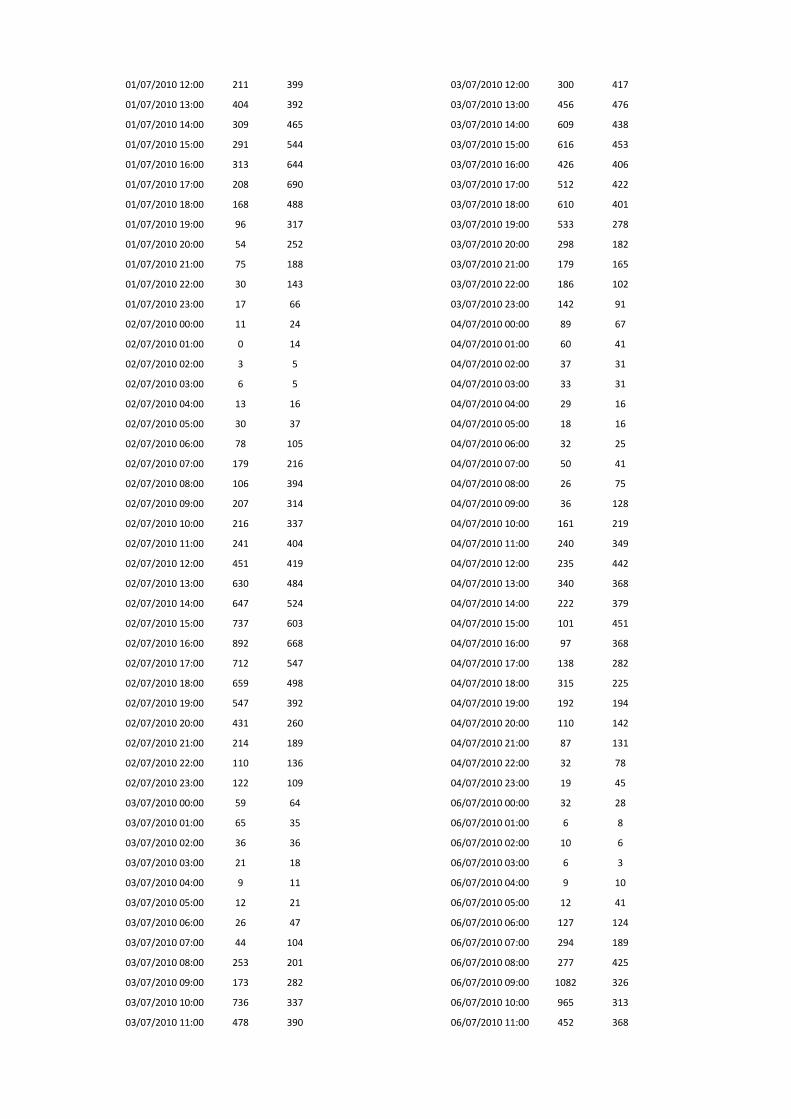
01/07/2010 12:00 211 399
01/07/2010 13:00 404 392
01/07/2010 14:00 309 465
01/07/2010 15:00 291 544
01/07/2010 16:00 313 644
01/07/2010 17:00 208 690
01/07/2010 18:00 168 488
01/07/2010 19:00 96 317
01/07/2010 20:00 54 252
01/07/2010 21:00 75 188
01/07/2010 22:00 30 143
01/07/2010 23:00 17 66
02/07/2010 00:00 11 24
02/07/2010 01:00 0 14
02/07/2010 02:00 3 5
02/07/2010 03:00 6 5
02/07/2010 04:00 13 16
02/07/2010 05:00 30 37
02/07/2010 06:00 78 105
02/07/2010 07:00 179 216
02/07/2010 08:00 106 394
02/07/2010 09:00 207 314
02/07/2010 10:00 216 337
02/07/2010 11:00 241 404
02/07/2010 12:00 451 419
02/07/2010 13:00 630 484
02/07/2010 14:00 647 524
02/07/2010 15:00 737 603
02/07/2010 16:00 892 668
02/07/2010 17:00 712 547
02/07/2010 18:00 659 498
02/07/2010 19:00 547 392
02/07/2010 20:00 431 260
02/07/2010 21:00 214 189
02/07/2010 22:00 110 136
02/07/2010 23:00 122 109
03/07/2010 00:00 59 64
03/07/2010 01:00 65 35
03/07/2010 02:00 36 36
03/07/2010 03:00 21 18
03/07/2010 04:00 9 11
03/07/2010 05:00 12 21
03/07/2010 06:00 26 47
03/07/2010 07:00 44 104
03/07/2010 08:00 253 201
03/07/2010 09:00 173 282
03/07/2010 10:00 736 337
03/07/2010 11:00 478 390
03/07/2010 12:00 300 417
03/07/2010 13:00 456 476
03/07/2010 14:00 609 438
03/07/2010 15:00 616 453
03/07/2010 16:00 426 406
03/07/2010 17:00 512 422
03/07/2010 18:00 610 401
03/07/2010 19:00 533 278
03/07/2010 20:00 298 182
03/07/2010 21:00 179 165
03/07/2010 22:00 186 102
03/07/2010 23:00 142 91
04/07/2010 00:00 89 67
04/07/2010 01:00 60 41
04/07/2010 02:00 37 31
04/07/2010 03:00 33 31
04/07/2010 04:00 29 16
04/07/2010 05:00 18 16
04/07/2010 06:00 32 25
04/07/2010 07:00 50 41
04/07/2010 08:00 26 75
04/07/2010 09:00 36 128
04/07/2010 10:00 161 219
04/07/2010 11:00 240 349
04/07/2010 12:00 235 442
04/07/2010 13:00 340 368
04/07/2010 14:00 222 379
04/07/2010 15:00 101 451
04/07/2010 16:00 97 368
04/07/2010 17:00 138 282
04/07/2010 18:00 315 225
04/07/2010 19:00 192 194
04/07/2010 20:00 110 142
04/07/2010 21:00 87 131
04/07/2010 22:00 32 78
04/07/2010 23:00 19 45
06/07/2010 00:00 32 28
06/07/2010 01:00 6 8
06/07/2010 02:00 10 6
06/07/2010 03:00 6 3
06/07/2010 04:00 9 10
06/07/2010 05:00 12 41
06/07/2010 06:00 127 124
06/07/2010 07:00 294 189
06/07/2010 08:00 277 425
06/07/2010 09:00 1082 326
06/07/2010 10:00 965 313
06/07/2010 11:00 452 368
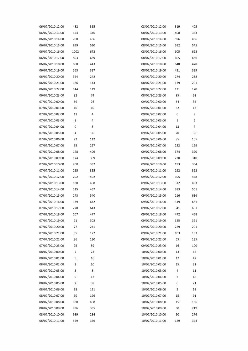
06/07/2010 12:00 482 365
06/07/2010 13:00 524 346
06/07/2010 14:00 708 466
06/07/2010 15:00 899 530
06/07/2010 16:00 1002 672
06/07/2010 17:00 803 669
06/07/2010 18:00 608 443
06/07/2010 19:00 563 337
06/07/2010 20:00 354 242
06/07/2010 21:00 186 143
06/07/2010 22:00 144 119
06/07/2010 23:00 82 74
07/07/2010 00:00 59 26
07/07/2010 01:00 16 10
07/07/2010 02:00 11 4
07/07/2010 03:00 8 4
07/07/2010 04:00 0 8
07/07/2010 05:00 4 30
07/07/2010 06:00 22 112
07/07/2010 07:00 55 227
07/07/2010 08:00 178 409
07/07/2010 09:00 174 309
07/07/2010 10:00 200 332
07/07/2010 11:00 265 355
07/07/2010 12:00 202 402
07/07/2010 13:00 180 408
07/07/2010 14:00 115 467
07/07/2010 15:00 273 540
07/07/2010 16:00 139 642
07/07/2010 17:00 228 643
07/07/2010 18:00 107 477
07/07/2010 19:00 71 302
07/07/2010 20:00 77 241
07/07/2010 21:00 55 172
07/07/2010 22:00 36 130
07/07/2010 23:00 25 59
08/07/2010 00:00 7 23
08/07/2010 01:00 5 16
08/07/2010 02:00 2 10
08/07/2010 03:00 3 8
08/07/2010 04:00 9 12
08/07/2010 05:00 2 38
08/07/2010 06:00 38 121
08/07/2010 07:00 60 196
08/07/2010 08:00 188 408
08/07/2010 09:00 936 335
08/07/2010 10:00 989 284
08/07/2010 11:00 559 356
08/07/2010 12:00 319 405
08/07/2010 13:00 408 383
08/07/2010 14:00 596 456
08/07/2010 15:00 612 545
08/07/2010 16:00 605 623
08/07/2010 17:00 605 666
08/07/2010 18:00 648 478
08/07/2010 19:00 431 339
08/07/2010 20:00 274 288
08/07/2010 21:00 179 201
08/07/2010 22:00 121 170
08/07/2010 23:00 95 62
09/07/2010 00:00 54 35
09/07/2010 01:00 32 13
09/07/2010 02:00 6 9
09/07/2010 03:00 1 5
09/07/2010 04:00 13 7
09/07/2010 05:00 20 35
09/07/2010 06:00 85 105
09/07/2010 07:00 232 199
09/07/2010 08:00 374 390
09/07/2010 09:00 220 310
09/07/2010 10:00 193 354
09/07/2010 11:00 292 322
09/07/2010 12:00 305 448
09/07/2010 13:00 312 493
09/07/2010 14:00 383 501
09/07/2010 15:00 216 616
09/07/2010 16:00 349 631
09/07/2010 17:00 341 601
09/07/2010 18:00 472 458
09/07/2010 19:00 325 321
09/07/2010 20:00 229 291
09/07/2010 21:00 103 193
09/07/2010 22:00 55 135
09/07/2010 23:00 16 100
10/07/2010 00:00 13 62
10/07/2010 01:00 17 47
10/07/2010 02:00 15 21
10/07/2010 03:00 4 11
10/07/2010 04:00 3 18
10/07/2010 05:00 6 21
10/07/2010 06:00 5 58
10/07/2010 07:00 15 91
10/07/2010 08:00 15 166
10/07/2010 09:00 30 219
10/07/2010 10:00 50 276
10/07/2010 11:00 129 394
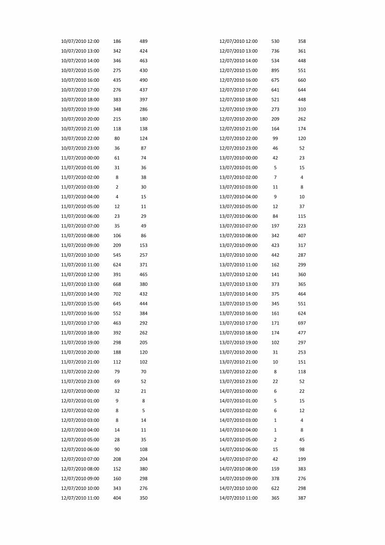
10/07/2010 12:00 186 489
10/07/2010 13:00 342 424
10/07/2010 14:00 346 463
10/07/2010 15:00 275 430
10/07/2010 16:00 435 490
10/07/2010 17:00 276 437
10/07/2010 18:00 383 397
10/07/2010 19:00 348 286
10/07/2010 20:00 215 180
10/07/2010 21:00 118 138
10/07/2010 22:00 80 124
10/07/2010 23:00 36 87
11/07/2010 00:00 61 74
11/07/2010 01:00 31 36
11/07/2010 02:00 8 38
11/07/2010 03:00 2 30
11/07/2010 04:00 4 15
11/07/2010 05:00 12 11
11/07/2010 06:00 23 29
11/07/2010 07:00 35 49
11/07/2010 08:00 106 86
11/07/2010 09:00 209 153
11/07/2010 10:00 545 257
11/07/2010 11:00 624 371
11/07/2010 12:00 391 465
11/07/2010 13:00 668 380
11/07/2010 14:00 702 432
11/07/2010 15:00 645 444
11/07/2010 16:00 552 384
11/07/2010 17:00 463 292
11/07/2010 18:00 392 262
11/07/2010 19:00 298 205
11/07/2010 20:00 188 120
11/07/2010 21:00 112 102
11/07/2010 22:00 79 70
11/07/2010 23:00 69 52
12/07/2010 00:00 32 21
12/07/2010 01:00 9 8
12/07/2010 02:00 8 5
12/07/2010 03:00 8 14
12/07/2010 04:00 14 11
12/07/2010 05:00 28 35
12/07/2010 06:00 90 108
12/07/2010 07:00 208 204
12/07/2010 08:00 152 380
12/07/2010 09:00 160 298
12/07/2010 10:00 343 276
12/07/2010 11:00 404 350
12/07/2010 12:00 530 358
12/07/2010 13:00 736 361
12/07/2010 14:00 534 448
12/07/2010 15:00 895 551
12/07/2010 16:00 675 660
12/07/2010 17:00 641 644
12/07/2010 18:00 521 448
12/07/2010 19:00 273 310
12/07/2010 20:00 209 262
12/07/2010 21:00 164 174
12/07/2010 22:00 99 120
12/07/2010 23:00 46 52
13/07/2010 00:00 42 23
13/07/2010 01:00 5 15
13/07/2010 02:00 7 4
13/07/2010 03:00 11 8
13/07/2010 04:00 9 10
13/07/2010 05:00 12 37
13/07/2010 06:00 84 115
13/07/2010 07:00 197 223
13/07/2010 08:00 342 407
13/07/2010 09:00 423 317
13/07/2010 10:00 442 287
13/07/2010 11:00 162 299
13/07/2010 12:00 141 360
13/07/2010 13:00 373 365
13/07/2010 14:00 375 464
13/07/2010 15:00 345 551
13/07/2010 16:00 161 624
13/07/2010 17:00 171 697
13/07/2010 18:00 174 477
13/07/2010 19:00 102 297
13/07/2010 20:00 31 253
13/07/2010 21:00 10 151
13/07/2010 22:00 8 118
13/07/2010 23:00 22 52
14/07/2010 00:00 6 22
14/07/2010 01:00 5 15
14/07/2010 02:00 6 12
14/07/2010 03:00 1 4
14/07/2010 04:00 1 8
14/07/2010 05:00 2 45
14/07/2010 06:00 15 98
14/07/2010 07:00 42 199
14/07/2010 08:00 159 383
14/07/2010 09:00 378 276
14/07/2010 10:00 622 298
14/07/2010 11:00 365 387

14/07/2010 12:00 265 386
14/07/2010 13:00 340 387
14/07/2010 14:00 285 455
14/07/2010 15:00 402 543
14/07/2010 16:00 501 654
14/07/2010 17:00 490 659
14/07/2010 18:00 510 484
14/07/2010 19:00 232 298
14/07/2010 20:00 133 256
14/07/2010 21:00 95 187
14/07/2010 22:00 51 145
14/07/2010 23:00 9 81
15/07/2010 00:00 6 30
15/07/2010 01:00 1 19
15/07/2010 02:00 2 5
15/07/2010 03:00 0 14
15/07/2010 04:00 3 11
15/07/2010 05:00 2 39
15/07/2010 06:00 19 104
15/07/2010 07:00 32 200
15/07/2010 08:00 88 376
15/07/2010 09:00 134 336
15/07/2010 10:00 205 308
15/07/2010 11:00 223 397
15/07/2010 12:00 197 417
15/07/2010 13:00 269 382
15/07/2010 14:00 301 459
15/07/2010 15:00 326 564
15/07/2010 16:00 191 663
15/07/2010 17:00 473 641
15/07/2010 18:00 391 478
15/07/2010 19:00 186 314
15/07/2010 20:00 43 253
15/07/2010 21:00 12 184
15/07/2010 22:00 8 131
15/07/2010 23:00 1 62
16/07/2010 00:00 3 35
16/07/2010 01:00 4 22
16/07/2010 02:00 8 11
16/07/2010 03:00 2 7
16/07/2010 04:00 4 7
16/07/2010 05:00 0 38
16/07/2010 06:00 25 116
16/07/2010 07:00 29 179
16/07/2010 08:00 62 420
16/07/2010 09:00 96 281
16/07/2010 10:00 107 335
16/07/2010 11:00 221 404
16/07/2010 12:00 169 428
16/07/2010 13:00 300 434
16/07/2010 14:00 314 486
16/07/2010 15:00 377 586
16/07/2010 16:00 683 657
16/07/2010 17:00 656 640
16/07/2010 18:00 697 439
16/07/2010 19:00 482 390
16/07/2010 20:00 256 266
27/07/2010 00:00 15 27
27/07/2010 01:00 5 14
27/07/2010 02:00 9 3
27/07/2010 03:00 6 9
27/07/2010 04:00 6 9
27/07/2010 05:00 6 39
27/07/2010 06:00 79 83
27/07/2010 07:00 95 166
27/07/2010 08:00 188 265
27/07/2010 09:00 257 261
27/07/2010 10:00 171 312
27/07/2010 11:00 342 371
27/07/2010 12:00 459 389
27/07/2010 13:00 610 413
27/07/2010 14:00 581 444
27/07/2010 15:00 626 575
27/07/2010 16:00 630 614
27/07/2010 17:00 604 670
27/07/2010 18:00 536 451
27/07/2010 19:00 440 332
27/07/2010 20:00 334 252
27/07/2010 21:00 198 175
27/07/2010 22:00 90 119
27/07/2010 23:00 76 55
28/07/2010 00:00 40 36
28/07/2010 01:00 23 24
28/07/2010 02:00 10 6
28/07/2010 03:00 7 9
28/07/2010 04:00 18 7
28/07/2010 05:00 23 40
28/07/2010 06:00 73 85
28/07/2010 07:00 168 184
28/07/2010 08:00 669 275
28/07/2010 09:00 917 256
28/07/2010 10:00 490 320
28/07/2010 11:00 248 393
28/07/2010 12:00 403 388
28/07/2010 13:00 290 375
28/07/2010 14:00 541 433

28/07/2010 15:00 515 505
28/07/2010 16:00 414 570
28/07/2010 17:00 580 633
28/07/2010 18:00 514 489
28/07/2010 19:00 312 343
28/07/2010 20:00 231 286
28/07/2010 21:00 153 190
28/07/2010 22:00 125 138
28/07/2010 23:00 102 76
29/07/2010 00:00 31 34
29/07/2010 01:00 16 22
29/07/2010 02:00 11 10
29/07/2010 03:00 8 9
29/07/2010 04:00 17 13
29/07/2010 05:00 9 33
29/07/2010 06:00 40 83
29/07/2010 07:00 106 153
29/07/2010 08:00 211 292
29/07/2010 09:00 180 299
29/07/2010 10:00 195 320
29/07/2010 11:00 345 348
29/07/2010 12:00 426 408
29/07/2010 13:00 431 413
29/07/2010 14:00 620 458
29/07/2010 15:00 610 539
29/07/2010 16:00 633 666
29/07/2010 17:00 730 647
29/07/2010 18:00 614 473
29/07/2010 19:00 450 341
29/07/2010 20:00 293 301
29/07/2010 21:00 216 211
29/07/2010 22:00 159 130
29/07/2010 23:00 78 67
30/07/2010 00:00 54 36
30/07/2010 01:00 29 21
30/07/2010 02:00 12 10
30/07/2010 03:00 14 8
30/07/2010 04:00 14 7
30/07/2010 05:00 10 40
30/07/2010 06:00 93 90
30/07/2010 07:00 177 175
30/07/2010 08:00 215 265
30/07/2010 09:00 184 287
30/07/2010 10:00 195 323
30/07/2010 11:00 333 396
30/07/2010 12:00 576 452
30/07/2010 13:00 472 460
30/07/2010 14:00 436 519
30/07/2010 15:00 386 565
30/07/2010 16:00 177 644
30/07/2010 17:00 80 586
30/07/2010 18:00 116 443
30/07/2010 19:00 62 341
30/07/2010 20:00 43 269
30/07/2010 21:00 9 200
30/07/2010 22:00 4 131
30/07/2010 23:00 4 97
31/07/2010 00:00 2 56
31/07/2010 01:00 3 26
31/07/2010 02:00 0 16
31/07/2010 03:00 2 15
31/07/2010 04:00 2 15
31/07/2010 05:00 8 15
31/07/2010 06:00 25 42
31/07/2010 07:00 46 96
31/07/2010 08:00 46 139
31/07/2010 09:00 63 199
31/07/2010 10:00 101 362
31/07/2010 11:00 174 421
31/07/2010 12:00 262 458
31/07/2010 13:00 392 483
31/07/2010 14:00 457 454
31/07/2010 15:00 465 490
31/07/2010 16:00 484 460
31/07/2010 17:00 522 435
31/07/2010 18:00 455 393
31/07/2010 19:00 382 295
31/07/2010 20:00 251 193
31/07/2010 21:00 125 178
31/07/2010 22:00 54 115
31/07/2010 23:00 34 79
01/08/2010 00:00 18 65
01/08/2010 01:00 21 50
01/08/2010 02:00 13 36
01/08/2010 03:00 19 29
01/08/2010 04:00 10 18
01/08/2010 05:00 9 19
01/08/2010 06:00 23 32
01/08/2010 07:00 21 61
01/08/2010 08:00 20 72
01/08/2010 09:00 22 115
01/08/2010 10:00 34 247
01/08/2010 11:00 108 336
01/08/2010 12:00 265 406
01/08/2010 13:00 438 420
01/08/2010 14:00 475 409

01/08/2010 15:00 423 433
01/08/2010 16:00 475 383
01/08/2010 17:00 393 247
01/08/2010 18:00 387 209
01/08/2010 19:00 307 178
01/08/2010 20:00 144 185
01/08/2010 21:00 141 109
01/08/2010 22:00 139 100
01/08/2010 23:00 70 48
02/08/2010 00:00 33 38
02/08/2010 01:00 19 8
02/08/2010 02:00 7 9
02/08/2010 03:00 14 7
02/08/2010 04:00 14 13
02/08/2010 05:00 31 28
02/08/2010 06:00 80 85
02/08/2010 07:00 144 144
02/08/2010 08:00 381 263
02/08/2010 09:00 662 273
02/08/2010 10:00 465 321
02/08/2010 11:00 663 342
02/08/2010 12:00 565 336
02/08/2010 14:00 836 441
02/08/2010 15:00 899 481
02/08/2010 16:00 810 609
02/08/2010 17:00 701 625
02/08/2010 18:00 566 443
02/08/2010 19:00 362 292
02/08/2010 20:00 226 244
02/08/2010 21:00 170 171
02/08/2010 22:00 160 135
02/08/2010 23:00 89 40
03/08/2010 00:00 31 20
03/08/2010 01:00 14 15
03/08/2010 02:00 6 9
03/08/2010 03:00 21 6
03/08/2010 04:00 5 4
03/08/2010 05:00 14 29
03/08/2010 06:00 95 99
03/08/2010 07:00 168 145
03/08/2010 08:00 143 259
03/08/2010 09:00 243 268
03/08/2010 10:00 198 275
03/08/2010 11:00 255 401
03/08/2010 12:00 267 395
03/08/2010 13:00 274 408
03/08/2010 14:00 414 429
03/08/2010 15:00 506 476
03/08/2010 16:00 515 614
03/08/2010 17:00 552 655
03/08/2010 18:00 620 496
03/08/2010 19:00 364 296
03/08/2010 20:00 278 242
03/08/2010 21:00 140 168
03/08/2010 22:00 108 103
03/08/2010 23:00 62 62
04/08/2010 00:00 33 19
04/08/2010 01:00 6 10
04/08/2010 02:00 3 6
04/08/2010 03:00 1 8
04/08/2010 04:00 8 10
04/08/2010 05:00 18 32
04/08/2010 06:00 83 84
04/08/2010 07:00 144 156
04/08/2010 08:00 149 295
04/08/2010 09:00 86 261
04/08/2010 10:00 291 349
04/08/2010 11:00 498 411
04/08/2010 12:00 418 398
04/08/2010 13:00 419 423
04/08/2010 14:00 474 452
04/08/2010 15:00 590 498
04/08/2010 16:00 762 628
04/08/2010 17:00 748 728
04/08/2010 18:00 584 463
04/08/2010 19:00 382 336
04/08/2010 20:00 265 244
04/08/2010 21:00 205 205
04/08/2010 22:00 205 124
04/08/2010 23:00 103 79
05/08/2010 00:00 52 33
05/08/2010 01:00 23 13
05/08/2010 02:00 17 16
05/08/2010 03:00 14 11
05/08/2010 04:00 13 12
05/08/2010 05:00 19 31
05/08/2010 06:00 52 80
05/08/2010 07:00 113 156
05/08/2010 08:00 486 269
05/08/2010 09:00 441 295
05/08/2010 10:00 344 340
05/08/2010 11:00 429 394
05/08/2010 12:00 398 397
05/08/2010 13:00 541 434
05/08/2010 14:00 820 471
05/08/2010 15:00 957 544

05/08/2010 16:00 854 601
05/08/2010 17:00 667 627
05/08/2010 18:00 587 502
05/08/2010 19:00 477 311
05/08/2010 20:00 316 298
05/08/2010 21:00 190 181
05/08/2010 22:00 151 159
05/08/2010 23:00 100 52
06/08/2010 00:00 43 34
06/08/2010 01:00 13 10
06/08/2010 02:00 4 10
06/08/2010 03:00 12 9
06/08/2010 04:00 11 7
06/08/2010 05:00 12 33
06/08/2010 06:00 72 82
06/08/2010 07:00 165 156
06/08/2010 08:00 180 286
06/08/2010 09:00 111 272
06/08/2010 10:00 84 321
06/08/2010 11:00 78 429
06/08/2010 12:00 147 447
06/08/2010 13:00 357 462
06/08/2010 14:00 186 528
06/08/2010 15:00 216 551
06/08/2010 16:00 187 609
06/08/2010 17:00 314 610
06/08/2010 18:00 167 478
06/08/2010 19:00 122 338
06/08/2010 20:00 70 261
06/08/2010 21:00 21 201
06/08/2010 22:00 23 140
06/08/2010 23:00 35 100
07/08/2010 00:00 8 76
07/08/2010 01:00 18 25
07/08/2010 02:00 7 20
07/08/2010 03:00 4 12
07/08/2010 04:00 2 12
07/08/2010 05:00 2 25
07/08/2010 06:00 15 47
07/08/2010 07:00 29 85
07/08/2010 08:00 31 135
07/08/2010 09:00 50 184
07/08/2010 10:00 61 326
07/08/2010 11:00 337 440
07/08/2010 12:00 411 430
07/08/2010 13:00 439 470
07/08/2010 14:00 491 425
07/08/2010 15:00 505 445
07/08/2010 16:00 713 454
07/08/2010 17:00 542 443
07/08/2010 18:00 463 372
07/08/2010 19:00 348 308
07/08/2010 20:00 265 210
07/08/2010 21:00 179 150
07/08/2010 22:00 81 117
07/08/2010 23:00 84 88
08/08/2010 00:00 49 62
08/08/2010 01:00 34 49
08/08/2010 02:00 42 41
08/08/2010 03:00 25 31
08/08/2010 04:00 16 19
08/08/2010 05:00 16 16
08/08/2010 06:00 28 20
08/08/2010 07:00 35 44
08/08/2010 08:00 46 77
08/08/2010 09:00 183 150
08/08/2010 10:00 349 276
08/08/2010 11:00 206 380
08/08/2010 12:00 271 429
08/08/2010 13:00 491 425
08/08/2010 14:00 486 415
08/08/2010 15:00 490 409
08/08/2010 16:00 442 356
08/08/2010 17:00 453 296
08/08/2010 18:00 426 236
08/08/2010 19:00 291 183
08/08/2010 20:00 208 185
08/08/2010 21:00 160 144
08/08/2010 22:00 123 67
08/08/2010 23:00 83 47
09/08/2010 00:00 39 17
09/08/2010 01:00 21 18
09/08/2010 02:00 9 9
09/08/2010 03:00 13 7
09/08/2010 04:00 10 12
09/08/2010 05:00 21 36
09/08/2010 06:00 78 80
09/08/2010 07:00 177 159
09/08/2010 08:00 274 282
09/08/2010 09:00 177 283
09/08/2010 10:00 129 276
09/08/2010 11:00 254 345
09/08/2010 12:00 228 403
09/08/2010 13:00 141 435
09/08/2010 14:00 130 416
09/08/2010 15:00 79 572

09/08/2010 16:00 242 713
09/08/2010 17:00 249 739
09/08/2010 18:00 157 465
09/08/2010 19:00 99 303
09/08/2010 20:00 21 210
09/08/2010 21:00 4 150
09/08/2010 22:00 9 113
09/08/2010 23:00 1 41
10/08/2010 00:00 0 28
10/08/2010 01:00 14 9
10/08/2010 02:00 3 7
10/08/2010 03:00 6 4
10/08/2010 04:00 4 7
10/08/2010 05:00 4 28
10/08/2010 06:00 24 87
10/08/2010 07:00 51 164
10/08/2010 08:00 173 302
10/08/2010 09:00 231 292
10/08/2010 10:00 305 244
10/08/2010 11:00 361 383
10/08/2010 12:00 411 362
10/08/2010 13:00 339 359
10/08/2010 14:00 288 488
10/08/2010 15:00 194 499
10/08/2010 16:00 397 603
10/08/2010 17:00 558 672
10/08/2010 18:00 538 459
10/08/2010 19:00 683 298
10/08/2010 20:00 386 271
10/08/2010 21:00 262 182
10/08/2010 22:00 105 187
10/08/2010 23:00 85 54
11/08/2010 00:00 25 30
11/08/2010 01:00 14 15
11/08/2010 02:00 10 3
11/08/2010 03:00 15 5
11/08/2010 04:00 10 8
11/08/2010 05:00 7 35
11/08/2010 06:00 56 75
11/08/2010 07:00 147 162
11/08/2010 08:00 258 280
11/08/2010 09:00 252 295
11/08/2010 10:00 679 372
11/08/2010 11:00 1008 397
11/08/2010 12:00 709 402
11/08/2010 13:00 352 375
11/08/2010 14:00 442 444
11/08/2010 15:00 532 517
11/08/2010 16:00 643 645
11/08/2010 17:00 665 696
11/08/2010 18:00 530 456
11/08/2010 19:00 446 347
11/08/2010 20:00 277 264
11/08/2010 21:00 152 207
11/08/2010 22:00 122 146
11/08/2010 23:00 101 80
12/08/2010 00:00 31 36
12/08/2010 01:00 17 15
12/08/2010 02:00 7 10
12/08/2010 03:00 9 6
12/08/2010 04:00 7 9
12/08/2010 05:00 22 40
12/08/2010 06:00 65 98
12/08/2010 07:00 143 178
12/08/2010 08:00 708 286
12/08/2010 09:00 656 285
12/08/2010 10:00 440 345
12/08/2010 11:00 450 385
12/08/2010 12:00 212 396
12/08/2010 13:00 284 432
12/08/2010 14:00 559 469
12/08/2010 15:00 460 555
12/08/2010 16:00 436 609
12/08/2010 17:00 471 663
12/08/2010 18:00 356 501
12/08/2010 19:00 343 329
12/08/2010 20:00 226 286
12/08/2010 21:00 130 207
12/08/2010 22:00 98 151
12/08/2010 23:00 88 73
13/08/2010 00:00 33 30
13/08/2010 01:00 22 13
13/08/2010 02:00 10 15
13/08/2010 03:00 11 4
13/08/2010 04:00 4 6
13/08/2010 05:00 20 40
13/08/2010 06:00 116 95
13/08/2010 07:00 193 172
13/08/2010 08:00 444 261
13/08/2010 09:00 772 254
13/08/2010 10:00 924 348
13/08/2010 11:00 769 391
13/08/2010 12:00 620 432
13/08/2010 13:00 564 451
13/08/2010 14:00 274 488
13/08/2010 15:00 254 607

13/08/2010 16:00 274 640
13/08/2010 17:00 512 610
13/08/2010 18:00 645 459
13/08/2010 19:00 372 358
13/08/2010 20:00 274 251
13/08/2010 21:00 54 226
13/08/2010 22:00 92 138
13/08/2010 23:00 86 74
14/08/2010 00:00 29 59
14/08/2010 01:00 28 34
14/08/2010 02:00 7 19
14/08/2010 03:00 9 19
14/08/2010 04:00 8 9
14/08/2010 05:00 14 25
14/08/2010 06:00 54 40
14/08/2010 07:00 59 113
14/08/2010 08:00 71 130
14/08/2010 09:00 74 194
14/08/2010 10:00 124 312
14/08/2010 11:00 629 417
14/08/2010 12:00 604 455
14/08/2010 13:00 355 449
14/08/2010 14:00 482 451
14/08/2010 15:00 404 458
14/08/2010 16:00 479 470
14/08/2010 17:00 444 484
14/08/2010 18:00 325 440
14/08/2010 19:00 361 248
14/08/2010 20:00 226 203
14/08/2010 21:00 133 148
14/08/2010 22:00 91 124
14/08/2010 23:00 55 76
15/08/2010 00:00 42 74
15/08/2010 01:00 42 48
15/08/2010 02:00 28 36
15/08/2010 03:00 58 36
15/08/2010 04:00 41 15
15/08/2010 05:00 18 19
15/08/2010 06:00 34 32
15/08/2010 07:00 72 48
15/08/2010 08:00 152 99
15/08/2010 09:00 313 129
15/08/2010 10:00 503 280
15/08/2010 11:00 864 400
15/08/2010 12:00 631 435
15/08/2010 13:00 404 381
15/08/2010 14:00 353 374
15/08/2010 15:00 340 424
15/08/2010 16:00 399 383
15/08/2010 17:00 330 290
15/08/2010 18:00 295 281
15/08/2010 19:00 248 207
15/08/2010 20:00 144 162
15/08/2010 21:00 115 155
15/08/2010 22:00 139 74
15/08/2010 23:00 72 39
16/08/2010 00:00 30 23
16/08/2010 01:00 19 13
16/08/2010 02:00 11 8
16/08/2010 03:00 14 9
16/08/2010 04:00 14 5
16/08/2010 05:00 18 39
16/08/2010 06:00 42 94
16/08/2010 07:00 157 172
16/08/2010 08:00 568 268
16/08/2010 09:00 920 287
16/08/2010 10:00 1042 333
16/08/2010 11:00 1233 378
16/08/2010 12:00 875 350
16/08/2010 13:00 452 359
16/08/2010 14:00 485 425
16/08/2010 15:00 588 518
16/08/2010 16:00 548 639
16/08/2010 17:00 564 654
16/08/2010 18:00 438 443
16/08/2010 19:00 282 293
16/08/2010 20:00 201 254
16/08/2010 21:00 137 173
16/08/2010 22:00 84 105
16/08/2010 23:00 53 47
17/08/2010 00:00 27 11
17/08/2010 01:00 7 11
17/08/2010 02:00 4 10
17/08/2010 03:00 14 6
17/08/2010 04:00 0 6
17/08/2010 05:00 18 44
17/08/2010 06:00 91 98
17/08/2010 07:00 147 158
17/08/2010 08:00 114 277
17/08/2010 09:00 70 256
17/08/2010 10:00 74 301
17/08/2010 11:00 125 392
17/08/2010 12:00 411 355
17/08/2010 13:00 440 377
17/08/2010 14:00 433 439
17/08/2010 15:00 634 518

17/08/2010 16:00 554 649
17/08/2010 17:00 617 682
17/08/2010 18:00 515 505
17/08/2010 19:00 319 278
17/08/2010 20:00 219 284
17/08/2010 21:00 167 182
17/08/2010 22:00 163 118
17/08/2010 23:00 54 42
18/08/2010 00:00 36 21
18/08/2010 01:00 13 12
18/08/2010 02:00 11 5
18/08/2010 03:00 10 9
18/08/2010 04:00 4 7
18/08/2010 05:00 16 38
18/08/2010 06:00 95 107
18/08/2010 07:00 143 170
18/08/2010 08:00 281 273
18/08/2010 09:00 736 291
18/08/2010 10:00 303 364
18/08/2010 11:00 338 414
18/08/2010 12:00 458 379
18/08/2010 13:00 483 374
18/08/2010 14:00 367 441
18/08/2010 15:00 268 533
18/08/2010 16:00 531 621
18/08/2010 17:00 780 741
18/08/2010 18:00 607 465
18/08/2010 19:00 294 318
18/08/2010 20:00 192 262
18/08/2010 21:00 190 200
18/08/2010 22:00 184 130
18/08/2010 23:00 67 60
19/08/2010 00:00 26 30
19/08/2010 01:00 14 20
19/08/2010 02:00 7 18
19/08/2010 03:00 7 7
19/08/2010 04:00 5 11
19/08/2010 05:00 20 29
19/08/2010 06:00 67 98
19/08/2010 07:00 79 161
19/08/2010 08:00 130 306
19/08/2010 09:00 127 293
19/08/2010 10:00 116 328
19/08/2010 11:00 346 386
19/08/2010 12:00 429 398
19/08/2010 13:00 295 412
19/08/2010 14:00 411 439
19/08/2010 15:00 480 535
19/08/2010 16:00 435 600
19/08/2010 17:00 276 661
19/08/2010 18:00 142 507
19/08/2010 19:00 37 295
19/08/2010 20:00 4 229
19/08/2010 21:00 6 166
19/08/2010 22:00 3 136
19/08/2010 23:00 5 59
20/08/2010 00:00 3 45
20/08/2010 01:00 6 19
20/08/2010 02:00 3 25
20/08/2010 03:00 5 14
20/08/2010 04:00 10 8
22/08/2010 09:00 96 153
22/08/2010 10:00 167 253
22/08/2010 11:00 270 341
22/08/2010 12:00 288 406
22/08/2010 13:00 317 380
22/08/2010 14:00 480 401
22/08/2010 15:00 470 419
22/08/2010 16:00 391 398
22/08/2010 17:00 440 336
22/08/2010 18:00 347 248
22/08/2010 19:00 305 168
22/08/2010 20:00 226 179
22/08/2010 21:00 153 115
22/08/2010 22:00 91 81
22/08/2010 23:00 43 41
23/08/2010 00:00 23 32
23/08/2010 01:00 13 14
23/08/2010 02:00 14 5
23/08/2010 03:00 6 10
23/08/2010 04:00 14 12
23/08/2010 05:00 10 27
23/08/2010 06:00 32 111
23/08/2010 07:00 93 171
23/08/2010 08:00 123 274
23/08/2010 09:00 440 246
23/08/2010 10:00 162 286
23/08/2010 11:00 98 371
23/08/2010 12:00 154 408
23/08/2010 13:00 246 421
23/08/2010 14:00 304 438
23/08/2010 15:00 438 496
23/08/2010 16:00 665 642
23/08/2010 17:00 693 647
23/08/2010 18:00 492 455
23/08/2010 19:00 284 271

23/08/2010 20:00 218 231
23/08/2010 21:00 214 181
23/08/2010 22:00 155 124
23/08/2010 23:00 62 55
24/08/2010 00:00 38 21
24/08/2010 01:00 10 11
24/08/2010 02:00 8 10
24/08/2010 03:00 4 8
24/08/2010 04:00 10 8
24/08/2010 05:00 13 33
24/08/2010 06:00 72 98
24/08/2010 07:00 214 164
24/08/2010 08:00 544 317
24/08/2010 09:00 391 349
24/08/2010 10:00 841 360
24/08/2010 11:00 1064 385
24/08/2010 12:00 682 396
24/08/2010 13:00 427 374
24/08/2010 14:00 557 484
24/08/2010 15:00 715 484
24/08/2010 16:00 657 666
24/08/2010 17:00 724 723
24/08/2010 18:00 585 497
24/08/2010 19:00 353 317
24/08/2010 20:00 236 235
24/08/2010 21:00 166 167
24/08/2010 22:00 79 128
24/08/2010 23:00 91 67
25/08/2010 00:00 28 39
25/08/2010 01:00 22 12
25/08/2010 02:00 4 12
25/08/2010 03:00 12 8
25/08/2010 04:00 15 12
25/08/2010 05:00 12 34
25/08/2010 06:00 60 87
25/08/2010 07:00 101 176
25/08/2010 08:00 150 258
25/08/2010 09:00 187 277
25/08/2010 10:00 184 319
25/08/2010 11:00 118 406
25/08/2010 12:00 121 401
25/08/2010 13:00 236 420
25/08/2010 14:00 293 446
25/08/2010 15:00 285 516
25/08/2010 16:00 279 609
25/08/2010 17:00 103 598
25/08/2010 18:00 78 479
25/08/2010 19:00 37 324
25/08/2010 20:00 12 233
25/08/2010 21:00 15 173
25/08/2010 22:00 7 130
25/08/2010 23:00 12 69
26/08/2010 00:00 5 34
26/08/2010 01:00 0 17
26/08/2010 02:00 3 9
26/08/2010 03:00 2 11
26/08/2010 04:00 3 10
26/08/2010 05:00 0 27
26/08/2010 06:00 17 102
26/08/2010 07:00 27 160
26/08/2010 08:00 76 275
26/08/2010 09:00 97 291
26/08/2010 10:00 149 312
26/08/2010 11:00 232 404
26/08/2010 12:00 298 393
26/08/2010 13:00 167 440
26/08/2010 14:00 186 459
26/08/2010 15:00 220 578
26/08/2010 16:00 258 685
26/08/2010 17:00 378 707
26/08/2010 18:00 233 519
26/08/2010 19:00 109 335
26/08/2010 20:00 80 284
26/08/2010 21:00 39 194
26/08/2010 22:00 33 141
26/08/2010 23:00 22 58
27/08/2010 00:00 11 31
27/08/2010 01:00 4 20
27/08/2010 02:00 6 6
27/08/2010 03:00 5 10
27/08/2010 04:00 6 7
27/08/2010 05:00 9 35
27/08/2010 06:00 26 106
27/08/2010 07:00 228 156
27/08/2010 08:00 671 265
27/08/2010 09:00 1000 319
27/08/2010 10:00 1103 374
27/08/2010 11:00 1189 426
27/08/2010 12:00 1046 453
27/08/2010 13:00 386 464
27/08/2010 14:00 507 519
27/08/2010 15:00 633 636
27/08/2010 16:00 671 635
27/08/2010 17:00 670 614
27/08/2010 18:00 493 497
27/08/2010 19:00 379 356

27/08/2010 20:00 375 290
27/08/2010 21:00 242 203
27/08/2010 22:00 160 144
27/08/2010 23:00 90 88
28/08/2010 00:00 61 48
28/08/2010 01:00 36 38
28/08/2010 02:00 24 21
28/08/2010 03:00 15 16
28/08/2010 04:00 15 17
28/08/2010 05:00 14 22
28/08/2010 06:00 35 41
28/08/2010 07:00 63 82
28/08/2010 08:00 76 163
28/08/2010 09:00 434 206
28/08/2010 10:00 796 345
28/08/2010 11:00 1074 436
28/08/2010 12:00 918 461
28/08/2010 13:00 465 455
28/08/2010 14:00 604 442
28/08/2010 15:00 509 395
28/08/2010 16:00 525 444
28/08/2010 17:00 529 479
28/08/2010 18:00 317 458
28/08/2010 19:00 286 261
28/08/2010 20:00 237 167
28/08/2010 21:00 152 163
28/08/2010 22:00 116 120
28/08/2010 23:00 69 72
29/08/2010 00:00 40 48
29/08/2010 01:00 53 31
29/08/2010 02:00 20 25
29/08/2010 03:00 23 29
29/08/2010 04:00 16 9
29/08/2010 05:00 5 13
29/08/2010 06:00 10 18
29/08/2010 07:00 6 53
29/08/2010 08:00 10 56
29/08/2010 09:00 10 127
29/08/2010 10:00 52 237
29/08/2010 11:00 40 378
29/08/2010 12:00 123 403
29/08/2010 13:00 241 365
29/08/2010 14:00 119 408
29/08/2010 15:00 296 400
29/08/2010 16:00 295 408
29/08/2010 17:00 518 271
29/08/2010 18:00 600 244
29/08/2010 19:00 463 199
29/08/2010 20:00 231 166
29/08/2010 21:00 160 143
29/08/2010 22:00 135 68
29/08/2010 23:00 49 56
30/08/2010 00:00 42 57
30/08/2010 01:00 32 42
30/08/2010 02:00 30 37
30/08/2010 03:00 24 31
30/08/2010 04:00 13 20
30/08/2010 05:00 12 15
30/08/2010 06:00 16 39
30/08/2010 07:00 44 56
30/08/2010 08:00 70 75
30/08/2010 09:00 179 154
30/08/2010 10:00 519 322
30/08/2010 11:00 1087 485
30/08/2010 12:00 1319 480
30/08/2010 13:00 694 465
30/08/2010 14:00 485 479
30/08/2010 15:00 635 489
30/08/2010 16:00 671 467
30/08/2010 17:00 643 361
30/08/2010 18:00 571 319
30/08/2010 19:00 421 247
30/08/2010 20:00 277 196
30/08/2010 21:00 221 155
30/08/2010 22:00 147 65
30/08/2010 23:00 42 47
31/08/2010 00:00 49 18
31/08/2010 01:00 10 5
31/08/2010 02:00 9 9
31/08/2010 03:00 15 4
31/08/2010 04:00 9 6
31/08/2010 05:00 9 24
31/08/2010 06:00 31 104
31/08/2010 07:00 125 148
31/08/2010 08:00 335 273
31/08/2010 09:00 862 272
31/08/2010 10:00 1025 344
31/08/2010 11:00 1321 420
31/08/2010 12:00 1228 391
31/08/2010 13:00 915 425
31/08/2010 14:00 751 478
31/08/2010 15:00 710 533
31/08/2010 16:00 565 622
31/08/2010 17:00 761 680
31/08/2010 18:00 1120 519
31/08/2010 19:00 785 343

31/08/2010 20:00 332 267
31/08/2010 21:00 231 190
31/08/2010 22:00 144 127
31/08/2010 23:00 64 65
01/09/2010 00:00 32 25
01/09/2010 01:00 19 11
01/09/2010 02:00 13 6
01/09/2010 03:00 8 13
01/09/2010 04:00 14 5
01/09/2010 05:00 7 33
01/09/2010 06:00 56 110
01/09/2010 07:00 150 208
01/09/2010 08:00 417 403
01/09/2010 09:00 854 291
01/09/2010 10:00 925 316
01/09/2010 11:00 1233 359
01/09/2010 12:00 1124 412
01/09/2010 13:00 647 426
01/09/2010 14:00 433 453
01/09/2010 15:00 627 563
01/09/2010 16:00 618 674
01/09/2010 17:00 856 674
01/09/2010 18:00 950 489
01/09/2010 19:00 661 365
01/09/2010 20:00 356 261
01/09/2010 21:00 259 185
01/09/2010 22:00 128 126
01/09/2010 23:00 86 67
02/09/2010 00:00 44 28
02/09/2010 01:00 13 10
02/09/2010 02:00 8 13
02/09/2010 03:00 13 14
02/09/2010 04:00 10 11
02/09/2010 05:00 12 40
02/09/2010 06:00 33 117
02/09/2010 07:00 151 191
02/09/2010 08:00 369 402
02/09/2010 09:00 1102 306
02/09/2010 10:00 1148 338
02/09/2010 11:00 1290 358
02/09/2010 12:00 1127 399
02/09/2010 13:00 779 396
02/09/2010 14:00 448 488
02/09/2010 15:00 455 561
02/09/2010 16:00 704 669
02/09/2010 17:00 902 667
02/09/2010 18:00 1020 514
02/09/2010 19:00 611 344
02/09/2010 20:00 302 285
02/09/2010 21:00 203 197
02/09/2010 22:00 155 113
02/09/2010 23:00 82 45
03/09/2010 00:00 34 27
03/09/2010 01:00 19 12
03/09/2010 02:00 11 10
03/09/2010 03:00 9 7
03/09/2010 04:00 6 12
03/09/2010 05:00 19 32
03/09/2010 06:00 80 100
03/09/2010 07:00 177 191
03/09/2010 08:00 470 423
03/09/2010 09:00 1069 307
03/09/2010 10:00 1136 323
03/09/2010 11:00 1050 430
03/09/2010 12:00 965 423
03/09/2010 13:00 521 460
03/09/2010 14:00 486 513
03/09/2010 15:00 586 655
03/09/2010 16:00 785 659
03/09/2010 17:00 765 592
03/09/2010 18:00 684 470
03/09/2010 19:00 517 351
03/09/2010 20:00 326 274
03/09/2010 21:00 192 162
03/09/2010 22:00 140 159
03/09/2010 23:00 86 91
04/09/2010 00:00 49 62
04/09/2010 01:00 50 26
04/09/2010 02:00 8 27
04/09/2010 03:00 10 17
04/09/2010 04:00 12 12
04/09/2010 05:00 11 23
04/09/2010 06:00 14 55
04/09/2010 07:00 62 96
04/09/2010 08:00 126 172
04/09/2010 09:00 433 274
04/09/2010 10:00 875 315
04/09/2010 11:00 1061 433
04/09/2010 12:00 740 501
04/09/2010 13:00 353 555
04/09/2010 14:00 238 462
04/09/2010 15:00 150 409
04/09/2010 16:00 461 497
04/09/2010 17:00 511 450
04/09/2010 18:00 571 411
04/09/2010 19:00 559 228

04/09/2010 20:00 174 175
04/09/2010 21:00 100 138
04/09/2010 22:00 71 120
04/09/2010 23:00 93 61
05/09/2010 00:00 55 61
05/09/2010 01:00 49 52
05/09/2010 02:00 56 24
05/09/2010 03:00 25 19
05/09/2010 04:00 5 9
05/09/2010 05:00 16 13
05/09/2010 06:00 15 26
05/09/2010 07:00 16 30
05/09/2010 08:00 8 69
05/09/2010 09:00 13 111
05/09/2010 10:00 67 228
05/09/2010 11:00 273 356
05/09/2010 12:00 112 431
05/09/2010 13:00 243 424
05/09/2010 14:00 145 452
05/09/2010 15:00 124 386
05/09/2010 16:00 131 401
05/09/2010 17:00 213 294
05/09/2010 18:00 138 227
05/09/2010 19:00 70 187
05/09/2010 20:00 140 148
05/09/2010 21:00 141 115
05/09/2010 22:00 137 73
05/09/2010 23:00 70 46
06/09/2010 00:00 52 15
06/09/2010 01:00 36 9
06/09/2010 02:00 25 7
06/09/2010 03:00 18 9
06/09/2010 04:00 20 13
06/09/2010 05:00 55 42
06/09/2010 06:00 151 94
06/09/2010 07:00 410 188
06/09/2010 08:00 549 374
06/09/2010 09:00 472 289
06/09/2010 10:00 91 266
06/09/2010 11:00 92 325
06/09/2010 12:00 118 398
06/09/2010 13:00 77 376
06/09/2010 14:00 64 404
06/09/2010 15:00 128 501
06/09/2010 16:00 162 617
06/09/2010 17:00 104 637
06/09/2010 18:00 32 437
06/09/2010 19:00 21 225
06/09/2010 20:00 18 227
06/09/2010 21:00 14 152
06/09/2010 22:00 6 95
06/09/2010 23:00 6 50
07/09/2010 00:00 10 22
07/09/2010 01:00 7 9
07/09/2010 02:00 2 5
07/09/2010 03:00 1 11
07/09/2010 04:00 11 10
07/09/2010 05:00 7 34
07/09/2010 06:00 54 119
07/09/2010 07:00 134 199
07/09/2010 08:00 139 421
07/09/2010 09:00 358 291
07/09/2010 10:00 302 300
07/09/2010 11:00 319 316
07/09/2010 12:00 269 364
07/09/2010 13:00 348 345
07/09/2010 14:00 476 452
07/09/2010 15:00 600 521
07/09/2010 16:00 696 644
07/09/2010 17:00 740 678
07/09/2010 18:00 494 466
07/09/2010 19:00 326 322
07/09/2010 20:00 208 263
07/09/2010 21:00 149 152
07/09/2010 22:00 95 102
07/09/2010 23:00 36 56

APPENDIX 5
MODIFIED ENTICE MODEL
<?php
//icemiser6.php
//ignore_user_abort(TRUE);// Previously left as ()
set_time_limit(600);// Important to prevent server timing out
// Sensitivity Analysis - 1 = ON, 0 = OFF
$LA = 1; $LW = 1; $SW = 1; $AL = 1; $RL = 1; $RC = 1; $TR = 1; $TOPO = 1; $PROX = 1; $TM = 0;
// Read in HOURLY forecast data
$IN = "ForecastData/".$SALTROUTE.".csv";
//echo $IN;
$HANDLE = fopen($IN, "r");
$DATA = fgetcsv($HANDLE, 1000, ",");
$JDAY = $DATA[0];$JMON = $DATA[1];$JYEAR = $DATA[2];
$DATA = fgetcsv($HANDLE, 1000, ",");
$RWIS = $DATA[0];
//$DATA = fgetcsv($HANDLE, 1000, ",");
//$SNOWLINE = $DATA[0];
$SNOWLINE = 1000;
$DATA = fgetcsv($HANDLE, 1000, ",");
$GROUND = $DATA[0];$SURF = $DATA[1];
$DATA = fgetcsv($HANDLE, 1000, ",");
$AT[0] = $DATA[0];$AT[1] = $DATA[1];$AT[2] = $DATA[2];$AT[3] = $DATA[3];$AT[4] = $DATA[4];
$AT[5] = $DATA[5];$AT[6] = $DATA[6];$AT[7] = $DATA[7];$AT[8] = $DATA[8];$AT[9] = $DATA[9];
$AT[10] = $DATA[10];$AT[11] = $DATA[11];$AT[12] = $DATA[12];$AT[13] = $DATA[13];$AT[14] =
$DATA[14];
$AT[15] = $DATA[15];$AT[16] = $DATA[16];$AT[17] = $DATA[17];$AT[18] = $DATA[18];$AT[19] =
$DATA[19];
$AT[20] = $DATA[20];$AT[21] = $DATA[21];$AT[22] = $DATA[22];$AT[23] = $DATA[23];$AT[24] =
$DATA[24];
//$AT[25] = $DATA[25];
$DATA = fgetcsv($HANDLE, 1000, ",");
$RF[0] = $DATA[0];$RF[1] = $DATA[1];$RF[2] = $DATA[2];$RF[3] = $DATA[3];$RF[4] = $DATA[4];
$RF[5] = $DATA[5];$RF[6] = $DATA[6];$RF[7] = $DATA[7];$RF[8] = $DATA[8];$RF[9] = $DATA[9];
$RF[10] = $DATA[10];$RF[11] = $DATA[11];$RF[12] = $DATA[12];$RF[13] = $DATA[13];$RF[14] =
$DATA[14];
$RF[15] = $DATA[15];$RF[16] = $DATA[16];$RF[17] = $DATA[17];$RF[18] = $DATA[18];$RF[19] =
$DATA[19];
$RF[20] = $DATA[20];$RF[21] = $DATA[21];$RF[22] = $DATA[22];$RF[23] = $DATA[23];$RF[24] =
$DATA[24];
//$RF[25] = $DATA[25];
$DATA = fgetcsv($HANDLE, 1000, ",");
$UI[0] = $DATA[0];$UI[1] = $DATA[1];$UI[2] = $DATA[2];$UI[3] = $DATA[3];
$UI[4] = $DATA[4];$UI[5] = $DATA[5];$UI[6] = $DATA[6];$UI[7] = $DATA[7];
$UI[8] = $DATA[8];$UI[9] = $DATA[9];$UI[10] = $DATA[10];$UI[11] = $DATA[11];
$UI[12] = $DATA[12];$UI[13] = $DATA[13];$UI[14] = $DATA[14];$UI[15] = $DATA[15];
$UI[16] = $DATA[16];$UI[17] = $DATA[17];$UI[18] = $DATA[18];$UI[19] = $DATA[19];
$UI[20] = $DATA[20];$UI[21] = $DATA[21];$UI[22] = $DATA[22];$UI[23] = $DATA[23];
$UI[24] = $DATA[24];
//$UI[25] = $DATA[25];
$DATA = fgetcsv($HANDLE, 1000, ",");
$RIN[0] = $DATA[0];$RIN[1] = $DATA[1];$RIN[2] = $DATA[2];$RIN[3] = $DATA[3];
$RIN[4] = $DATA[4];$RIN[5] = $DATA[5];$RIN[6] = $DATA[6];$RIN[7] = $DATA[7];
$RIN[8] = $DATA[8];$RIN[9] = $DATA[9];$RIN[10] = $DATA[10];$RIN[11] = $DATA[11];
$RIN[12] = $DATA[12];$RIN[13] = $DATA[13];$RIN[14] = $DATA[14];$RIN[15] = $DATA[15];
$RIN[16] = $DATA[16];$RIN[17] = $DATA[17];$RIN[18] = $DATA[18];$RIN[19] = $DATA[19];
$RIN[20] = $DATA[20];$RIN[21] = $DATA[21];$RIN[22] = $DATA[22];$RIN[23] = $DATA[23];
$RIN[24] = $DATA[24];
//$RIN[25] = $DATA[25];

$DATA = fgetcsv($HANDLE, 1000, ",");
$IA[0] = $DATA[0];$IA[1] = $DATA[1];$IA[2] = $DATA[2];$IA[3] = $DATA[3];
$IA[4] = $DATA[4];$IA[5] = $DATA[5];$IA[6] = $DATA[6];$IA[7] = $DATA[7];
$IA[8] = $DATA[8];$IA[9] = $DATA[9];$IA[10] = $DATA[10];$IA[11] = $DATA[11];
$IA[12] = $DATA[12];$IA[13] = $DATA[13];$IA[14] = $DATA[14];$IA[15] = $DATA[15];
$IA[16] = $DATA[16];$IA[17] = $DATA[17];$IA[18] = $DATA[18];$IA[19] = $DATA[19];
$IA[20] = $DATA[20];$IA[21] = $DATA[21];$IA[22] = $DATA[22];$IA[23] = $DATA[23];
$IA[24] = $DATA[24];
//$IA[25] = $DATA[25];
$DATA = fgetcsv($HANDLE, 1000, ",");
$IT[0] = $DATA[0];$IT[1] = $DATA[1];$IT[2] = $DATA[2];$IT[3] = $DATA[3];
$IT[4] = $DATA[4];$IT[5] = $DATA[5];$IT[6] = $DATA[6];$IT[7] = $DATA[7];
$IT[8] = $DATA[8];$IT[9] = $DATA[9];$IT[10] = $DATA[10];$IT[11] = $DATA[11];
$IT[12] = $DATA[12];$IT[13] = $DATA[13];$IT[14] = $DATA[14];$IT[15] = $DATA[15];
$IT[16] = $DATA[16];$IT[17] = $DATA[17];$IT[18] = $DATA[18];$IT[19] = $DATA[19];
$IT[20] = $DATA[20];$IT[21] = $DATA[21];$IT[22] = $DATA[22];$IT[23] = $DATA[23];
$IT[24] = $DATA[24];
//$IT[25] = $DATA[25];
$DATA = fgetcsv($HANDLE, 1000, ",");
$WINDIR[0] = $DATA[0];$WINDIR[1] = $DATA[1];$WINDIR[2] = $DATA[2];$WINDIR[3] = $DATA[3];
$WINDIR[4] = $DATA[4];$WINDIR[5] = $DATA[5];$WINDIR[6] = $DATA[6];$WINDIR[7] = $DATA[7];
$WINDIR[8] = $DATA[8];$WINDIR[9] = $DATA[9];$WINDIR[10] = $DATA[10];$WINDIR[11] = $DATA[11];
$WINDIR[12] = $DATA[12];$WINDIR[13] = $DATA[13];$WINDIR[14] = $DATA[14];$WINDIR[15] =
$DATA[15];
$WINDIR[16] = $DATA[16];$WINDIR[17] = $DATA[17];$WINDIR[18] = $DATA[18];$WINDIR[19] =
$DATA[19];
$WINDIR[20] = $DATA[20];$WINDIR[21] = $DATA[21];$WINDIR[22] = $DATA[22];$WINDIR[23] =
$DATA[23];
$WINDIR[24] = $DATA[24];
// Convert date to Julian day
$JUDY[0] = 31; $JUDY[1] = 59; $JUDY[2] = 90;
$JUDY[3] = 120; $JUDY[4] = 151; $JUDY[5] = 181;
$JUDY[6] = 212; $JUDY[7] = 243; $JUDY[8] = 273;
$JUDY[9] = 304; $JUDY[10] = 334;
$TOY = $JDAY;
for ($I = 1; $I<=11; $I++)
{
$INDEX = $I - 1;
if ($JMON == ($I+1)) {$TOY = $JUDY[$INDEX]+$JDAY;}
}
$MODRESULT = $JDAY % 4;
if (($JMON > 2) && ($MODRESULT == 0)) {$TOY = $TOY + 1;}
$LEAP = 12;
for ($I = 1950; $I<($JYEAR + 1); $I++)
{
$MODRESULT = $I % 4;
if ($MODRESULT == 0) {$LEAP = $LEAP + 1;}
}
$DAYS = (($JYEAR - 1900) * 365.0) + $LEAP + $TOY - 0.5;
// Interpolate wind, cloud and rain data
// Values are averaged linearly for the 20 minute intervals between input values.
for ($I = 1; $I<=72; $I++)
{
if((($I+2)/3) == INTVAL(($I+2)/3)) // HOURLY DATA
{
$INDEX=(INTVAL(($I+2)/3))-1;
$UA[$I]=($UI[$INDEX]*45)+90;
$IC[$I]=$IA[$INDEX];
$IH[$I]=$IT[$INDEX];
$RFALL[$I]=$RIN[$INDEX];
$WDIR[$I]=$WINDIR[$INDEX];
$INDEX1=$INDEX+1;
} ELSE {
if(($I/3) == INTVAL(($I+2)/3)) // 20 PAST HOUR
{
$UA[$I]=(($UI[$INDEX]+(($UI[$INDEX1]-$UI[$INDEX])/1.5))*45)+90;
$IC[$I]=INTVAL($IA[$INDEX]+(($IA[$INDEX1]-$IA[$INDEX])/1.5));
$IH[$I]=INTVAL($IT[$INDEX]+(($IT[$INDEX1]-$IT[$INDEX])/1.5));

$RFALL[$I]=INTVAL($RIN[$INDEX]+(($RIN[$INDEX1]-
$RIN[$INDEX])/1.5));
$WDIR[$I]=INTVAL($WINDIR[$INDEX]+(($WINDIR[$INDEX1]-
$WINDIR[$INDEX])/1.5));
} ELSE { //40 PAST HOUR
$UA[$I]=(($UI[$INDEX]+(($UI[$INDEX1]-$UI[$INDEX])/3))*45)+90;
$IC[$I]=INTVAL($IA[$INDEX]+(($IA[$INDEX1]-$IA[$INDEX])/3));
$IH[$I]=INTVAL($IT[$INDEX]+(($IT[$INDEX1]-$IT[$INDEX])/3));
$RFALL[$I]=INTVAL($RIN[$INDEX]+(($RIN[$INDEX1]-
$RIN[$INDEX])/3));
$WDIR[$I]=INTVAL($WINDIR[$INDEX]+(($WINDIR[$INDEX1]-
$WINDIR[$INDEX])/3));
}
}
//echo "winddir=$WDIR[$I]<br>";
// Calculate stability class
if (($IH[$I] == 3) && ($IC[$I] > 5)) {$IC[$I] = 4;}
if (($UA[$I] < 181) && ($IC[$I] < 4))
{
$STABILITYCLASS[$I] = 1;
$ELR[$I] = 0.0;
} elseif (($UA[$I] < 226) && ($UA[$I] > 180) && ($IC[$I] < 5))
{
$STABILITYCLASS[$I] = 2;
$ELR[$I] = 0.003;
} elseif (($UA[$I] < 226) && ($IC[$I] > 4))
{
$STABILITYCLASS[$I] = 3;
$ELR[$I] = 0.006;
} elseif (($UA[$I] < 316) && ($UA[$I] > 225) && ($IC[$I] < 5))
{
$STABILITYCLASS[$I] = 3;
$ELR[$I] = 0.006;
} else
{
$STABILITYCLASS[$I] = 4;
$ELR[$I] = 0.009;
}
}
// Parameterise cloud data for use in the radiation balance
for ($J = 1; $J<=72; $J++)
{
if (($IC[$J] >= 1) && ($IC[$J] <= 7))
{
if ($IH[$J] == 1)
{
if (($IC[$J] >= 1) && ($IC[$J] <= 2)) {$X[$J] = 0.2; $Y[$J] = 0.6;
$Z[$J] = 0.87;}
if (($IC[$J] >= 3) && ($IC[$J] <= 5)) {$X[$J] = 0.5; $Y[$J] = 0.8;
$Z[$J] = 0.58;}
if ($IC[$J] > 5) {$X[$J] = 0.9; $Y[$J] = 1.0; $Z[$J] = 0.32;}
} elseif ($IH[$J] == 2)
{
if (($IC[$J] >= 1) && ($IC[$J] <= 2)) {$X[$J] = 0.1; $Y[$J] = 0.6;
$Z[$J] = 0.91;}
if (($IC[$J] >= 3) && ($IC[$J] <= 5)) {$X[$J] = 0.3; $Y[$J] = 0.8;
$Z[$J] = 0.72;}
if ($IC[$J] > 5) {$X[$J] = 0.9; $Y[$J] = 1.3; $Z[$J] = 0.54;}
} else
{
if (($IC[$J] >= 1) && ($IC[$J] <= 2)) {$X[$J] = 0.05; $Y[$J] = 0.5;
$Z[$J] = 0.96;}
if (($IC[$J] >= 3) && ($IC[$J] <= 5)) {$X[$J] = 0.1; $Y[$J] = 0.5;
$Z[$J] = 0.86;}
if ($IC[$J] > 5) {$X[$J] = 0.3; $Y[$J] = 0.6; $Z[$J] = 0.78;}
}
}
if ($IC[$J] == 0) {$X[$J] = 0; $Y[$J] = 0.5; $Z[$J] = 1;}
if ($IC[$J] == 8)
{
$X[$J] = 1; $Y[$J] = 1; $Z[$J] = 0.78;
if ($IH[$J] == 1) {$Z[$J] = 0.32;}
if ($IH[$J] == 2) {$Z[$J] = 0.54;}

}
$ALBED[$J] = $X[$J];
$DPLUS[$J] = $Y[$J];
$KCLOU[$J] = $Z[$J];
}
// Create empty route forecast database
$DBFNAME1 = "TemperatureDataQC/".$SALTROUTE.".dbf";
$DBFNAME2 = "ConditionDataQC/".$SALTROUTE.".dbf";
//$DBFNAME1 = "$OUT1.dbf";
//$DBFNAME2 = "$OUT2.dbf";
$DEF = array(
array("X","N",12,2),
array("Y","N",12,2),
array("1200","N",12,2),
array("1220","N",12,2),
array("1240","N",12,2),
array("1300","N",12,2),
array("1320","N",12,2),
array("1340","N",12,2),
array("1400","N",12,2),
array("1420","N",12,2),
array("1440","N",12,2),
array("1500","N",12,2),
array("1520","N",12,2),
array("1540","N",12,2),
array("1600","N",12,2),
array("1620","N",12,2),
array("1640","N",12,2),
array("1700","N",12,2),
array("1720","N",12,2),
array("1740","N",12,2),
array("1800","N",12,2),
array("1820","N",12,2),
array("1840","N",12,2),
array("1900","N",12,2),
array("1920","N",12,2),
array("1940","N",12,2),
array("2000","N",12,2),
array("2020","N",12,2),
array("2040","N",12,2),
array("2100","N",12,2),
array("2120","N",12,2),
array("2140","N",12,2),
array("2200","N",12,2),
array("2220","N",12,2),
array("2240","N",12,2),
array("2300","N",12,2),
array("2320","N",12,2),
array("2340","N",12,2),
array("0000","N",12,2),
array("0020","N",12,2),
array("0040","N",12,2),
array("0100","N",12,2),
array("0120","N",12,2),
array("0140","N",12,2),
array("0200","N",12,2),
array("0220","N",12,2),
array("0240","N",12,2),
array("0300","N",12,2),
array("0320","N",12,2),
array("0340","N",12,2),
array("0400","N",12,2),
array("0420","N",12,2),
array("0440","N",12,2),
array("0500","N",12,2),
array("0520","N",12,2),
array("0540","N",12,2),
array("0600","N",12,2),
array("0620","N",12,2),
array("0640","N",12,2),
array("0700","N",12,2),
array("0720","N",12,2),
array("0740","N",12,2),
array("0800","N",12,2),
array("0820","N",12,2),

array("0840","N",12,2),
array("0900","N",12,2),
array("0920","N",12,2),
array("0940","N",12,2),
array("1000","N",12,2),
array("1020","N",12,2),
array("1040","N",12,2),
array("1100","N",12,2),
array("1120","N",12,2),
array("1140","N",12,2)
);
//dbase_create($DBF_RST_ROUTE_MAKE,$DEF);
//dbase_create($DBF_RSC_ROUTE_MAKE,$DEF);
$RSTDBF = dbase_create($DBFNAME1,$DEF);
$CONDBF = dbase_create($DBFNAME2,$DEF);
// Specify array - check if needed since $REC specified when data written to route database
//$REC = array($SITE[0], $SITE[1], $SITE[2], $SITE[3], $SITE[4], $SITE[5], $SITE[6], $SITE[7],
$SITE[8], $SITE[9], //$SITE[10], $SITE[11], $SITE[12], $SITE[13], $SITE[14], $SITE[15],
$SITE[16], $SITE[17], $SITE[18], $SITE[19], //$SITE[20], $SITE[21], $SITE[22], $SITE[23],
$SITE[24], $SITE[25]);
// Specify constants
$RDA = 0.00694;
$RDC = 0.012;
$RDS = 0.004;
//$ZG = 72.0; //commented out since $ZG is now variable based on GPR measurements
$PI = 3.141592654;
$RADEG = 360 / (2 * $PI);
// Start spatial loop
// Open the salting route database and read in data
if ($FETCH == 1)
{
$IN = "SaltingRoutes/Bham_PhDzo100.dbf";
}
elseif ($FETCH == 2)
{
$IN = "SaltingRoutes/Bham_PhDzo150.dbf";
}
elseif ($FETCH == 3)
{
$IN = "SaltingRoutes/Bham_PhDzo200.dbf";
}
elseif ($FETCH == 4)
{
$IN = "SaltingRoutes/Bham_PhDzo250.dbf";
}
elseif ($FETCH == 5)
{
$IN = "SaltingRoutes/Bham_PhDzo500GPR.dbf";//added GPR to end of filename
}
else
{
echo "error - no salting route databse found!";
}
//$IN = "SaltingRoutes/Bham_PhD.dbf";
//echo $IN;
$DB = dbase_open($IN,2);
$NR = dbase_numrecords($DB);
for ($M = 1; $M<=$NR; $M++)
{
$SITE = dbase_get_record($DB,$M);
$EASTING[$M] = $SITE[1];
$NORTHING[$M] = $SITE[2];
$LATITUDE[$M] = $SITE[3];
//$LONGITUDE[$M] = $SITE[4];
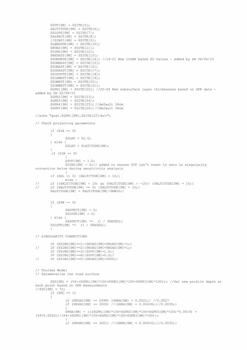
$SVF[$M] = $SITE[5];
$ALTITUDE[$M] = $SITE[6];
$SLOPE[$M] = $SITE[7];
$ASPECT[$M] = $SITE[8];
//$CAPI[$M] = $SITE[9];
$LANDUSE[$M] = $SITE[10];
$ROAD[$M] = $SITE[11];
$SING[$M] = $SITE[12];
$RESRST[$M] = $SITE[13];
$ZONORTH[$M] = $SITE[14]; //14-21 New LIDAR based ZO values - added by DH 04/06/10
$ZONEAST[$M] = $SITE[15];
$ZOEAST[$M] = $SITE[16];
$ZOSEAST[$M] = $SITE[17];
$ZOSOUTH[$M] = $SITE[18];
$ZOSWEST[$M] = $SITE[19];
$ZOWEST[$M] = $SITE[20];
$ZONWEST[$M] = $SITE[21];
$GPR1[$M] = $SITE[22]; //22-24 New subsurface layer thicknesses based on GPR data -
added by DH 22/08/10
$GPR2[$M] = $SITE[23];
$GPR3[$M] = $SITE[24];
$GPR4[$M] = $SITE[25]; //default 18cm
$GPR5[$M] = $SITE[26]; //default 36cm
//echo "goat.$GPR1[$M],$SITE[22]<br>";
// Check projecting parameters
if ($LA == 0)
{
$SLAT = 52.5;
} else {
$SLAT = $LATITUDE[$M];
}
if ($LW == 0)
{
$SVF[$M] = 1.0;
$SING[$M] = 0;// added to ensure SVF isn't reset to zero in singularity
correction below during sensitivity analysis
}
if ($AL == 0) {$ALTITUDE[$M] = 10;}
else {
// if (($ALTITUDE[$M] < 10) && ($ALTITUDE[$M] > -10)) {$ALTITUDE[$M] = 10;}
// if ($ALTITUDE[$M] == 0) {$ALTITUDE[$M] = 10;}
$ALTITUDE[$M] = $ALTITUDE[$M]-$RWIS;}
if ($SW == 0)
{
$ASPECT[$M] = 0;
$SLOPE[$M] = 0;
} else {
$ASPECT[$M] *= (1 / $RADEG);
$SLOPE[$M] *= (1 / $RADEG);
}
// SINGULARITY CORRECTIONS
IF ($SING[$M]==1){$ROAD[$M]=$ROAD[$M]+1;}
// IF ($SING[$M]==2){$ROAD[$M]=$ROAD[$M]+1;}
IF ($SING[$M]==3){$SVF[$M]=1.0;}
IF ($SING[$M]==4){$SVF[$M]=0.0;}
// IF ($SING[$M]==5){$ROAD[$M]=3000;}
// Thornes Model
// Parameterise the road surface
$ZG[$M] = (54+($GPR1[$M]*100+$GPR2[$M]*100+$GPR3[$M]*100)); //Set new profile depth at
each point based on GPR measurements
//$ZG[$M] = 72;
if ($RC == 1)
{
if ($ROAD[$M] == 2999) {$RKA[$M] = 0.0021;} //0.0027
if ($ROAD[$M] == 3000) //{$RKA[$M] = 0.00438;}//0.0039;}
{
$RKA[$M] = ((($GPR1[$M]*100+$GPR2[$M]*100+$GPR3[$M]*100)*0.0019) +
(54*0.0052))/(54+($GPR1[$M]*100+$GPR2[$M]*100+$GPR3[$M]*100));
}
if ($ROAD[$M] == 3001) //{$RKA[$M] = 0.00410;}//0.0035;}

{
$RKA[$M] = ((($GPR1[$M]*100+$GPR2[$M]*100+$GPR3[$M]*100)*0.0019) + (18*0.0052)
+ ((36*0.8)*0.0052) + ((36*0.2)*0.0024))/(54+($GPR1[$M]*100+$GPR2[$M]*100+$GPR3[$M]*100));
}
if ($ROAD[$M] == 3002) //{$RKA[$M] = 0.00409;}//0.0029;} //0.0031
{
$RKA[$M] = ((($GPR1[$M]*100+$GPR2[$M]*100)*0.0019) +
((($GPR3[$M]*100)+18)*0.0052) + ((36*0.5)*0.0052) +
((36*0.5)*0.0024))/(54+($GPR1[$M]*100+$GPR2[$M]*100+$GPR3[$M]*100));
}
if ($ROAD[$M] == 3004) //{$RKA[$M] = 0.00359;}//0.0022;} //0.0027
{
$RKA[$M] = ((($GPR1[$M]*100)*0.0019) +
((($GPR2[$M]*100+$GPR3[$M]*100)+18)*0.0052) +
(36*0.0024))/(54+($GPR1[$M]*100+$GPR2[$M]*100+$GPR3[$M]*100));
}
} else {$RKA[$M] = ((($GPR1[$M]*100+$GPR2[$M]*100+$GPR3[$M]*100)*0.0019) +
(54*0.0052))/(54+($GPR1[$M]*100+$GPR2[$M]*100+$GPR3[$M]*100));}//0.00438;}//0.0039;}
//$fi = fopen('gpr_depth.csv', 'w');
//fputcsv($fi,$RKA,',');
//fclose($fp);
//$FRED[$M] = $GPR1[$M]*100+$GPR2[$M]*100+$GPR3[$M]*100;
//echo "goat.$RKA[$M],$FRED[$M]<br>";
if ($TR == 1)
{
if ($ROAD[$M] == 2999) {$TRAF = 0.85;}
if ($ROAD[$M] == 3000) {$TRAF = 0.85;}
if ($ROAD[$M] == 3001) {$TRAF = 0.9;}
if ($ROAD[$M] == 3002) {$TRAF = 0.95;}
if ($ROAD[$M] == 3004) {$TRAF = 1.0;}
if ($LANDUSE[$M] > 3) {$TRAF = 0.85;}
} else {$TRAF = 1.0;}
// if ($RL == 1)
// {
// if ($LANDUSE[$M] == 1) {$ZO[$M] = 25;}
// if ($LANDUSE[$M] == 2) {$ZO[$M] = 50;}
// if ($LANDUSE[$M] == 3) {$ZO[$M] = 50;}
// if ($LANDUSE[$M] == 4) {$ZO[$M] = 75;}
// if ($LANDUSE[$M] == 5) {$ZO[$M] = 100;}
// if (($LANDUSE[$M] == 1) && ($ROAD[$M] <= 3000)) {$ZO[$M] = 50;}
// } else {$ZO[$M] = 15;}
if ($RL == 1)
{
// Select the correct LIDAR ZO dataset based on wind direction
//$ZO[$M] = 1;
for ($I = 1; $I<=72; $I++)
{
if ($WDIR[$I] < 22.5 or $WDIR[$I] > 337.5)
{
$ZO[$M] = $ZONORTH[$M]*100;
}
elseif ($WDIR[$I] >= 22.5 and $WDIR[$I] < 67.5)
{
$ZO[$M] = $ZONEAST[$M]*100;
}
elseif ($WDIR[$I] >= 67.5 and $WDIR[$I] < 112.5)
{
$ZO[$M] = $ZOEAST[$M]*100;
}
elseif ($WDIR[$I] >= 112.5 and $WDIR[$I] < 157.5)
{
$ZO[$M] = $ZOSEAST[$M]*100;
}
elseif ($WDIR[$I] >= 157.5 and $WDIR[$I] < 202.5)
{
$ZO[$M] = $ZOSOUTH[$M]*100;
}
elseif ($WDIR[$I] >= 202.5 and $WDIR[$I] < 247.5)
{
$ZO[$M] = $ZOSWEST[$M]*100;
}
elseif ($WDIR[$I] >= 247.5 and $WDIR[$I] < 292.5)
{

$ZO[$M] = $ZOWEST[$M]*100;
}
elseif ($WDIR[$I] >= 292.5 and $WDIR[$I] <= 337.5)
{
$ZO[$M] = $ZONWEST[$M]*100;
}
else
{
$ZO[$M] = $ZOWEST[$M]*100;
}
}
$ZO[$M] = $ZOWEST[$M] * 100;
//echo "$LANDUSE[$M],$ZO[$M]<br>";
for ($I = 1; $I<=72; $I++)
{
// Where LIDAR ZO values are missing (-999900), replace with original ZO value based on
ordinal classification
if ($ZO[$M] == -999900)
{
if ($LANDUSE[$M] == 1)
{
$ZO[$M] = 15;
}
elseif ($LANDUSE[$M] == 2 or $LANDUSE[$M] == 3)
{
$ZO[$M] = 50;
}
elseif ($LANDUSE[$M] == 4)
{
$ZO[$M] = 70;
}
elseif ($LANDUSE[$M] == 5)
{
$ZO[$M] = 100;
}
elseif ($LANDUSE[$M] == 1 and $ROAD[$M] <= 3000)
{
$ZO[$M] = 50;
}
else
{
$ZO[$M] = 15;
}
}
elseif ($ZO[$M] <= 15)
{
$ZO[$M] = 15;
}
elseif ($ZO[$M] > 15 and $ZO[$M] <= 25)////start of
extra//////////////////////////////////////////////////
{
$ZO[$M] = 20;
}
elseif ($ZO[$M] > 25 and $ZO[$M] <= 35)
{
$ZO[$M] = 30;
}
elseif ($ZO[$M] > 35 and $ZO[$M] <= 45)
{
$ZO[$M] = 40;
}
elseif ($ZO[$M] > 45 and $ZO[$M] <= 55)
{
$ZO[$M] = 50;
}
elseif ($ZO[$M] > 55 and $ZO[$M] <= 65)
{
$ZO[$M] = 60;
}
elseif ($ZO[$M] > 65 and $ZO[$M] <= 75)
{
$ZO[$M] = 70;
}
elseif ($ZO[$M] > 75 and $ZO[$M] <= 85)
{
$ZO[$M] = 80;

}
elseif ($ZO[$M] > 85 and $ZO[$M] <= 95)
{
$ZO[$M] = 90;
}
elseif ($ZO[$M] > 95 and $ZO[$M] <= 105)
{
$ZO[$M] = 100;
}
elseif ($ZO[$M] > 105 and $ZO[$M] <= 115)
{
$ZO[$M] = 110;
}
elseif ($ZO[$M] > 115 and $ZO[$M] <= 125)
{
$ZO[$M] = 120;
}
elseif ($ZO[$M] > 125 and $ZO[$M] <= 135)
{
$ZO[$M] = 130;
}
elseif ($ZO[$M] > 135 and $ZO[$M] <= 145)
{
$ZO[$M] = 140;
}
elseif ($ZO[$M] > 145)
{
$ZO[$M] = 150;
}
else
{
$ZO[$M] = $ZO[$M];
}
}
} else {$ZO[$M] = 15;}
//echo "$LANDUSE[$M],$ZO[$M]<br>";
// $fi = fopen('lidar_zo.csv', 'w');
// fputcsv($fi,$ZO,',');
// Convert temps to Kelvin scale and correct with ALTITUDE
// Looks inefficient - can temp and dew point be read in at the same time as cloud earlier in
code
for ($I = 1; $I<=72; $I++)
{
if((($I+2)/3) == INTVAL(($I+2)/3)) // HOURLY DATA
{
$INDEX=(INTVAL(($I+2)/3))-1;
$ATA[$I]=$AT[$INDEX];
$V[$I]=$RF[$INDEX];
$INDEX1=$INDEX+1;
} ELSE {
if(($I/3) == INTVAL(($I+2)/3)) // 20 PAST HOUR DATA
{
$ATA[$I]=$AT[$INDEX]+(($AT[$INDEX1]-$AT[$INDEX])/1.5);
$V[$I]=$RF[$INDEX]+(($RF[$INDEX1]-$RF[$INDEX])/1.5);
} ELSE { // 40 PAST HOUR DATA
$ATA[$I]=$AT[$INDEX]+(($AT[$INDEX1]-$AT[$INDEX])/3);
$V[$I]=$RF[$INDEX]+(($RF[$INDEX1]-$RF[$INDEX])/3);
}
}
$AELR = $ALTITUDE[$M] * $ELR[$I];
$TA[$I] = $ATA[$I] - $AELR;
$V[$I] = $V[$I] - $AELR;
$TA[$I] = $TA[$I] + 273.16;
$V[$I] = $V[$I] + 273.16;
$DP[$I][$M] = $V[$I] - 273.16;
$V[$I] = SHMB($V[$I],$TA[$I]);
$RHF[$I] = $V[$I] / SHMB($TA[$I],$TA[$I]);
$W[$I] = 1.5 * $V[$I] + 0.6;
// if ($I == 1)
// {
$ZA[$I] = ZAIR($UA[$I],$ZO[$M]);
$EXCO[$I] = ((POW(0.4,2)) * 0.001 * $UA[$I]) / (POW((LOG($ZA[$I] /
$ZO[$M])),2));
// }

// else
// {
// $ZA[$I] = $ZA[$I - 1];
// $EXCO[$I] = $EXCO[$I - 1];
// }
}
// Generate incoming radiation
for ($I = 1; $I<=72; $I++)
{
$ALBED1 = $ALBED[$I];
$DPLUS1 = $DPLUS[$I];
$INDEX = $I + 36;
$J = $INDEX % 72;
if ($J == 0) {$J = 72;}
$TIME[$I] = ($J-1)/3;
$INDEX = $I-1;
if (($INDEX % 3) == 0)
{
$MIN=$I-1;
LIST($DEC,$R) = SUNDEC($DAYS,$TIME[1],$MIN,$RADEG);
}
list ($COSZ,$COSTHETA,$VFVAL) =
COSAZI($I,$J,$RADEG,$SLAT,$DEC,$SLOPE[$M],$ASPECT[$M]);
// $BUL = (($PI / 2) - ((($VFMAT($VFVAL, $M)) * $PI) / 100)) *
$RADEG;
$BUL = (($PI / 2) - ((50 * $PI) / 100)) * $RADEG;
list ($SUN[$I],$ALBEDO[$I],$COSZ,$COSTHETA,$ALT[$I]) =
SUNGEN($COSZ,$W[$I],$R,$ALBED1,$DPLUS1,$BUL,$COSTHETA,$RADEG);
}
// Parameterise rainfall
// Note that as the original parameters were 500 and 1000 for light and heavy rain
respectively over 3 hour periods,
// the new parameters of 50 and 100 are applied to the new 20 minute forecast interval.
// These figures can be tweaked if needed.
$RAIN = 0;
$SHRF = 0;
$SNO = 0;
for ($I = 1; $I<=72; $I++)
{
if ($RFALL[$I] == 0) {$RAIN = $RAIN;}
if (($I == 1) && ($RIN[1] == 1)) {$RAIN = 50;}
if (($I == 1) && ($RIN[1] == 2)) {$RAIN = 100;}
if (($I == 1) && ($RIN[1] == 3)) {$RAIN = 100;} // SNOW
if ($RFALL[$I] == 1){$RAIN = $RAIN+50;$SNO = 0;}
if ($RFALL[$I] == 2){$RAIN = $RAIN+100;$SNO = 0;}
if ($RFALL[$I] == 3){$RAIN = $RAIN+100;$SNO = 1;}
if ($RAIN > 0) {$SHRF = 1;}
$PRECIPITATION = $RAIN;
$SNOW = $SNO;
// Interval halving algorithm and longwave generation
$K = 0;
$Z1 = $TA[$I] - 10;
$Z2 = $TA[$I] + 10;
$SHWO[0] = 0;
do
{
$K=$K+1;
if ($K == 1) {$T[$I] = $Z1;}
if ($K == 2) {$T[$I] = $Z2;}
if ($K > 2)
{
$INDEX1 = $K-1;
$INDEX2 = $K-2;
$T[$I]= $TE[$INDEX1] - (($TE[$INDEX1] - $TE[$INDEX2]) *
$SHWO[$INDEX1]) / ($SHWO[$INDEX1] - $SHWO[$INDEX2]);

}
$TE[$K] = $T[$I];
$KCLOU1 = $KCLOU[$I];
$RNLONG = ((0.95*(BB($T[$I])))*$SVF[$M])-((BB($TA[$I]))*((0.82-
0.25*(POW(10,(-0.094*$V[$I]))))));
$RN[$I] = (1.0 - $ALBEDO[$I]) * $SUN[$I] - $RNLONG * $KCLOU1 * $TRAF;
// Road construction and introduce lag
if ($RC == 1)
{
$RCONS[$M] = $ROAD[$M];
} else {
$RCONS[$M] = 3000;
}
if ($I == 1)
{
$ZT = $ZG[$M] / ($ZG[$M]/($ZG[$M]-36));//2;
$ZZ = $ZT / ($ZT/($ZT-18));//2;
$ZX = $ZZ / ($ZZ/($ZZ-$GPR3[$M]*100));//2;
$ZU = $ZX / ($ZX/($ZX-$GPR2[$M]*100));//2;
//echo "$ZT,$ZZ,$ZX,$ZU,$LANDUSE[$M]<br>";
$TT[$I] = ($GROUND + 273.16); //$TA(I) THIS IS THE TEMP AT 36CM,
TZ IS 18CM
$TZ[$I] = ($TT[$I] + $T[$I]) / 2;//($ZT/$ZZ);//2;//18cm
$TX[$I] = ($TZ[$I] + $T[$I]) / 2;//($ZZ/$ZX);//2;//9cm
$TU[$I] = ($TX[$I] + $T[$I]) / 2;//($ZX/$ZU);//2;//5cm
$TG = $TU[$I];
// $vartz=($ZG[$M]/$ZT);
// $vartx=$ZZ/$ZX;
// $vartu=$ZX/$ZU;
//echo "$TT[$I],$TZ[$I],$TX[$I],$TU[$I],$T[$I]<br>";//,$vartx,$vartu,$TT<br>";
$S[$I] = (0.00438 / $ZG[$M]) * ($TU[$I] - $T[$I]) *
60000;//changed conductivity from 0.0039(original entice motorway av) to new motorway average
(0.00438)
} else {
$INDEX4 = $I-1;
if (($RCONS[$M] >= 3002) && ($LANDUSE[$M] == 1))
{
$TT[$I] = $TT[$INDEX4] + $RDS * (($T[$INDEX4] - 2 *
$TT[$INDEX4] + $TG) / ($ZT * $ZT)) * 1.2E3;
} else {
$TT[$I] = $TT[$INDEX4] + $RDC * (($T[$INDEX4] - 2 *
$TT[$INDEX4] + $TG) / ($ZT * $ZT)) * 1.2E3;
}
$TZ[$I] = $TZ[$INDEX4] + $RDC * (($T[$INDEX4] - 2 * $TZ[$INDEX4]
+ $TT[$INDEX4]) / ($ZZ * $ZZ)) * 1.2E3;
if (($RCONS[$M] == 3000) OR ($RCONS[$M] == 3001))
{
$TX[$I] = $TX[$INDEX4] + $RDA * (($T[$INDEX4] - 2 *
$TX[$INDEX4] + $TZ[$INDEX4]) / ($ZX * $ZX)) * 1.2E3;
} else {
$TX[$I] = $TX[$INDEX4] + $RDC * (($T[$INDEX4] - 2 *
$TX[$INDEX4] + $TZ[$INDEX4]) / ($ZX * $ZX)) * 1.2E3;
}
if ($RCONS[$M] == 2999)
{
$TU[$I] = $TU[$INDEX4] + $RDC * (($T[$INDEX4] - 2 *
$TU[$INDEX4] + $TX[$INDEX4]) / ($ZU * $ZU)) * 1.2E3;
} else {
$TU[$I] = $TU[$INDEX4] + $RDA * (($T[$INDEX4] - 2 *
$TU[$INDEX4] + $TX[$INDEX4]) / ($ZU * $ZU)) * 1.2E3;
}
$S[$I] = ($RKA[$M] / $ZU) * ($TU[$I] - $T[$I]) * 60000;
}
$EXXO[$I] = $EXCO[$I] * RIFIX($TA[$I], $T[$I], $ZA[$I], $ZO[$M],
$UA[$I]);
$H[$I] = $EXXO[$I] * 0.24 * ($TA[$I] + 0.0001 * $ZA[$I] - $T[$I]) *
60000;
$QGRAD = Q($TA[$I],$RHF[$I]) - Q($T[$I],1);
//echo "$TT[$I],$TZ[$I],$TX[$I],$TU[$I],$T[$I]<br>";
// Dew falls everywhere
if ($QGRAD > 0)
{

$LE[$I] = $EXXO[$I] * 590 * $QGRAD * 60000;
} else {
$LE[$I] = $EXXO[$I] * 590 * $QGRAD * 60000 * $SHRF;
}
$SHWO[$K] = $RN[$I]+$S[$I]+$H[$I]+$LE[$I];
} while (($SHWO[$K] > 1) OR ($SHWO[$K] < -1));
$RAIN = $RAIN + $LE[$I];
// if (($TA[$I] < $DP[$I]) && ($DP[$I] < 273.16)) {$RAIN = $RAIN + 500;} //HOAR
FROST
if ($RAIN < 0)
{
$SHRF = 0;
$RAIN = 0;
}
// Convert surface temperature to Celsius
$TC[$I] = $T[$I] - 273.16;
$T18[$I] = $TZ[$I] - 273.16;
$T9[$I] = $TX[$I] - 273.16;
$T5[$I] = $TU[$I] - 273.16;
$T35[$I] = $TT[$I] - 273.16;
$TA[$I] = $TA[$I] - 273.16;
// $TA[$I] -= 273.16;
$TD[1] = $SURF;
$INDEX5=($I-1);
if ($I > 1)
{
$TD[$I] = $TC[$I] + ($TD[$INDEX5] - $TC[$I]) / 2;
//Traffic correction
if (($TR == 1) && ($ROAD[$M] > 3000))
{
$TD[$I] = $TD[$I] - 1;
if ($LANDUSE[$M] == 5)
{
// DEAL WITH DIFFERENCE BTWN MWAY AND A ROAD DUAL CARRIAGEWAY (SING=5)
// IF ($SING[$M]==5)
// {$TD[$I] += 0.75;}ELSE{
if ($ROAD[$M] == 3001) {$TD[$I] += 0.5;}
if ($ROAD[$M] == 3002) {$TD[$I] += 0.5;}
if ($ROAD[$M] == 3004) {$TD[$I] += 0.4;}
// }
}
if ($LANDUSE[$M] == 4)
{
if ($ROAD[$M] == 3001) {$TD[$I] += 0.5;}
if ($ROAD[$M] == 3002) {$TD[$I] += 0.4;}
if ($ROAD[$M] == 3004) {$TD[$I] += 0.3;}
}
if ($LANDUSE[$M] == 3)
{
if ($ROAD[$M] == 3001) {$TD[$I] += 0.4;}
if ($ROAD[$M] == 3002) {$TD[$I] += 0.3;}
if ($ROAD[$M] == 3004) {$TD[$I] += 0.2;}
}
if ($LANDUSE[$M] == 2)
{
if ($ROAD[$M] == 3001) {$TD[$I] += 0.3;}
if ($ROAD[$M] == 3002) {$TD[$I] += 0.2;}
if ($ROAD[$M] == 3004) {$TD[$I] += 0.1;}
}
if ($LANDUSE[$M] == 1)
{
if ($ROAD[$M] == 3001) {$TD[$I] += 0.2;}
if ($ROAD[$M] == 3002) {$TD[$I] += 0.1;}
}
}
// Topography correction
if ($TOPO == 1) {}

// Proximity correction
if ($PROX == 1) {}
}
// Condition parameters
if ($PRECIPITATION == "0")
{
$CONDITION[$I] = 0;
} else {
$CONDITION[$I] = 1;
}
if ($TD[$I] < $DP[$I][$M]) {$CONDITION[$I] = 1;}
if (($PRECIPITATION == "0") && ($RAIN > 0)) {$CONDITION[$I] = 1;}
if (($TD[$I] < 0) && ($CONDITION[$I] = 1)) {$CONDITION[$I] = 2;}
// if (($SNOW == 1) && ($TD[$I] < 2) && ($ALTITUDE[$M] > $SNOWLINE))
{$CONDITION[$I] = 3;}
if (($SNOW == 1) && ($TD[$I] < 2)) {$CONDITION[$I] = 3;}
// Check for rounding error
if (($TD[$I] < 0)&&($TD[$I] > -0.1)){$TD[$I]=-0.1;}
if (($TD[$I] > 0)&&($TD[$I] < 0.1)){$TD[$I]=0.1;}
//echo "$WDIR[$I]<br>";
} // End temporal loop
// Write RST to route database
$REC = array($EASTING[$M], $NORTHING[$M], $TD[1], $TD[2], $TD[3], $TD[4], $TD[5],
$TD[6], $TD[7], $TD[8], $TD[9], $TD[10], $TD[11], $TD[12], $TD[13], $TD[14], $TD[15], $TD[16],
$TD[17], $TD[18], $TD[19], $TD[20], $TD[21], $TD[22], $TD[23], $TD[24], $TD[25], $TD[26],
$TD[27], $TD[28], $TD[29], $TD[30], $TD[31], $TD[32], $TD[33], $TD[34], $TD[35], $TD[36],
$TD[37], $TD[38], $TD[39], $TD[40], $TD[41], $TD[42], $TD[43], $TD[44], $TD[45], $TD[46],
$TD[47], $TD[48], $TD[49], $TD[50], $TD[51], $TD[52], $TD[53], $TD[54], $TD[55], $TD[56],
$TD[57], $TD[58], $TD[59], $TD[60], $TD[61], $TD[62], $TD[63], $TD[64], $TD[65], $TD[66],
$TD[67], $TD[68], $TD[69], $TD[70], $TD[71], $TD[72]);
dbase_add_record($RSTDBF,$REC);
// Write RSC to route database
$REC = array($EASTING[$M], $NORTHING[$M], $CONDITION[1], $CONDITION[2], $CONDITION[3],
$CONDITION[4], $CONDITION[5], $CONDITION[6], $CONDITION[7], $CONDITION[8], $CONDITION[9],
$CONDITION[10], $CONDITION[11], $CONDITION[12], $CONDITION[13], $CONDITION[14],
$CONDITION[15], $CONDITION[16], $CONDITION[17], $CONDITION[18], $CONDITION[19],
$CONDITION[20], $CONDITION[21], $CONDITION[22], $CONDITION[23], $CONDITION[24],
$CONDITION[25], $CONDITION[26], $CONDITION[27], $CONDITION[28], $CONDITION[29],
$CONDITION[30], $CONDITION[31], $CONDITION[32], $CONDITION[33], $CONDITION[34],
$CONDITION[35], $CONDITION[36], $CONDITION[37], $CONDITION[38], $CONDITION[39],
$CONDITION[40], $CONDITION[41], $CONDITION[42], $CONDITION[43], $CONDITION[44],
$CONDITION[45], $CONDITION[46], $CONDITION[47], $CONDITION[48], $CONDITION[49],
$CONDITION[50], $CONDITION[51], $CONDITION[52], $CONDITION[53], $CONDITION[54],
$CONDITION[55], $CONDITION[56], $CONDITION[57], $CONDITION[58], $CONDITION[59],
$CONDITION[60], $CONDITION[61], $CONDITION[62], $CONDITION[63], $CONDITION[64],
$CONDITION[65], $CONDITION[66], $CONDITION[67], $CONDITION[68], $CONDITION[69],
$CONDITION[70], $CONDITION[71], $CONDITION[72]);
dbase_add_record($CONDBF,$REC);
//echo "$ZO[$M]<br>";
}
// End spatial loop
dbase_close($DB);
dbase_close($RSTDBF);
dbase_close($CONDBF);
echo "Route Forecast Complete<br><br>";
?>