the use of advertising activities to meet earnings ...€¦ · advertising spending to achieve the...
TRANSCRIPT

The use of advertising activities to meet earnings benchmarks:
Evidence from monthly data*
Daniel Cohen Stern School of Business
New York University 44 West 4th Street
New York, NY 10012 (212) 998-0267
Raj Mashruwala Olin Business School
Washington University in St. Louis Campus Box 1133
One Brookings Drive St. Louis, MO 63130-4899
(314) 935-5924 [email protected]
Tzachi Zach
Olin Business School Washington University in St. Louis
Campus Box 1133 One Brookings Drive
St. Louis, MO 63130-4899 (314) 935-4528 [email protected]
First Draft: August 2007 Current Draft: November 2007
* We gratefully acknowledge the financial support of the Center for Research in Economics and Strategy at the Olin School of Business. We have benefited from the comments of Eli Bartov, Anne Beatty, Messod Beneish, Larry Brown, Donal Byard, Masako Darrough, Richard Dietrich, Nick Dopuch, Richard Frankel, April Klein, Thomas Lys, Christina Mashruwala, Shamin Mashruwala, Shail Pandit, Kristi Schneck, Amy Zang, Paul Zarowin, Jerry Zimmerman, participants at the 2007 Conference of Financial Economics and Accounting and at the 2007 Nick Dopuch Conference, and workshop participants at Baruch College, Georgia State University, George Washington University, University of Illinois, The Ohio State University, Penn State University, Southern Methodist University and Washington University in St. Louis.

The use of advertising activities to meet earnings benchmarks: Evidence from monthly data
Abstract
Using a unique and comprehensive data set of monthly information on advertising spending in media outlets, we examine whether managers engage in real earnings management to meet quarterly financial reporting benchmarks. We extend prior literature by: (1) examining quarterly as opposed to annual earnings benchmarks and separating advertising from other expenses, which allows us to incorporate advertising’s unique characteristics; (2) exploring the possibility that managers could either reduce or boost advertising to increase chances of meeting an earnings benchmark; (3) investigating the timing, within a fiscal quarter, of altered advertising spending; and (4) analyzing actual activities as opposed to inferring them from reported expenses, which could also be influenced by accrual choices. Our analysis suggests that managers reduce their advertising spending to achieve the financial reporting goals of avoiding losses, avoiding earnings decrease, and meeting analysts’ forecasts. We find some evidence that advertising spending increases during the third month of a fiscal quarter. This increase is stronger for managers who have incentives to meet earnings benchmarks and whose firms have higher margins. We find no evidence of an increased tendency to alter advertising spending after the Sarbanes-Oxley Act.

1
The use of advertising activities to meet earnings benchmarks: Evidence from monthly data
1. Introduction
Extensive evidence shows that managers engage in earnings management
activities (for reviews of the evidence, see Healy and Wahlen [1999], Kothari [2001], and
Fields, Lys, and Vincent [2001]). The literature to date identifies two main strategies to
manage reported earnings: (i) accounting method changes and accrual-based earnings
management that do not affect cash flows and (ii) real actions taken by managers that
affect cash flows. The early evidence on earnings management concentrates on accrual-
based strategies. More recently, Graham, Harvey, and Rajgopal [2005], in a survey of top
executives, report that 80% of respondents would decrease discretionary spending (such
as research and development and advertising) to achieve financial reporting objectives.
Consistent with the survey, large sample evidence suggests that managers engage in real
earnings management to avoid reporting annual losses (Roychowdhury [2006]). These
actions have implications for future firm performance (Gunny [2005]) and are viewed as
substitutes to accrual-based strategies (Zang [2006]).
While top executives recognize the importance of altering advertising activities as
a means to achieve certain financial reporting objectives, large-scale empirical evidence
to support this assertion does not exist. The literature to date has focused on other real
activities, such as research and development, asset sales, and overproduction. Studies
have only included advertising expenses (when they were available) as part of aggregate
discretionary expenses. Given the economic importance of this item in a firm’s business
strategy, we fill the void in the literature by analyzing it separately.

2
In this paper, we address the following research questions: (i) do managers use
advertising activities to meet certain earnings benchmarks? (ii) are there circumstances in
which managers will increase (rather than decrease) advertising activities to meet these
benchmarks?, and (iii) is there a specific time during a fiscal period in which altering
advertising activities to achieve financial reporting goals is more likely to occur?
To answer these questions we employ a data set of monthly advertising activities,
because these questions cannot be answered with data available on Compustat. Our study
contributes to the literature on real earnings management by extending it along several
dimensions. First, our high-frequency data on advertising enable us to focus on a specific
item that is subject to managerial discretion in order to meet quarterly earnings
benchmarks — the benchmarks that the extant literature on meeting financial reporting
benchmarks has mostly investigated (DeGeorge, Patell, and Zeckhauser [1999], Brown
and Caylor [2005]). Survey evidence in Graham, Harvey, and Rajgopal [2005] also
confirms that managers care about quarterly performance and benchmark beating. But
because information on advertising expenses in Compustat is only available on an annual
basis, analyzing managerial decisions about advertising expenses to meet quarterly
benchmarks was not possible until now.
In addition, prior studies generally aggregate the annual advertising expense
together with other discretionary expenses such as research and development and
maintenance, or as part of selling and general expenses. For example, Roychowdhury
[2006] aggregates several items, such as R&D, SG&A, and advertising, into a single
annual measure of discretionary expenses. Zang [2006] and Gunny [2005] separately
analyze a finer set of annual variables that proxy for real earnings management, which

3
include abnormal levels of R&D, SG&A, production costs, and gains from asset sales.
McNichols [2003] discusses the importance of disaggregating empirical measures of
accounting choices in the context of accrual-based earnings management. Focusing on a
single item provides a more powerful setting for the analysis and allows the exploration
of richer theories about managerial actions that may vary depending on the item subject
to discretion.
Our second contribution is exploring the possibility that managers increase (and
not decrease) their advertising activities to attain certain accounting benchmarks. Prior
studies have assumed that reducing discretionary expenses (including advertising)
directly maps into a contemporaneous increase in reported earnings. However, because
reduced advertising can quickly lower revenues in some cases, it is not clear whether
reducing advertising activities will always be beneficial to managers. The marketing
literature suggests that there is a variation across firms and products in the lead-lag
relation between advertising activities and sales (Assmus, Farley and Lehmann, 1984).
That is, for some firms advertising activities may trigger an immediate response in sales,
while for others, advertising will generate the desired impact after a longer period. This
raises the possibility that in some cases managers may choose to increase advertising to
increase sales and short-term earnings, rather than decrease advertising only to lower
expenses. Thus, the relation between advertising and reported income may be ambiguous.
Our comprehensive monthly data also allow us to study the timing of managerial
choices regarding real activities, which is the third contribution of our study. This aspect,
too, could not be achieved with existing large-scale data available through Compustat.
Altering real activities, such as advertising, involves a tradeoff between two time

4
considerations. On the one hand, managers are interested in taking actions early in the
fiscal period to ensure that their financial effects will be reflected by the time the fiscal
period ends. In this way, the probability of achieving the desired financial reporting
objective is increased. On the other hand, managers would like to postpone real actions as
much as possible, to acquire more information about the firm’s expected financial
performance for the period and about the magnitude of action needed to meet certain
benchmarks. This learning minimizes the negative consequences of altering real
activities. By examining high-frequency data, we are able to identify the month in which
real earnings management may take place.
Fourth, our data are extracted from direct observation of advertising activities in a
wide range of media outlets. According to GAAP, these advertising activities are
expensed as incurred. This enables us to directly examine managerial actions that have
immediate financial statement consequences. In contrast, prior studies that examine real
earnings management rely on income statement expenses. These expenses, however,
could be affected by accrual choices. These studies implicitly assume a one-to-one
correspondence between real actions and the observed accounting figures. However, this
assumption may not necessarily hold, especially in samples of firms that have incentives
to achieve certain financial reporting objectives. Thus, prior evidence is subject to the
alternative explanation that accrual choices (for example, aggressive capitalizations)
affect the level of expenses, rather than the real choices made by managers.
Summary of the results. We find strong evidence that firms reduce their
advertising spending in order to meet all three types of financial reporting objectives we
examine — avoiding reporting a loss, meeting earnings from the same quarter in the

5
previous year, and meeting analysts’ forecasts or beating them by one cent. Utilizing the
distinctive features of our high-frequency data, we find weaker evidence that there is an
increase in abnormal advertising activities in the third month of a fiscal quarter.
However, this increase is not limited to “suspect” firms, i.e., firms that have just met the
three financial reporting objectives. One exception is that we do find evidence of
increased advertising activities to meet analysts’ forecasts during the third month of the
fiscal quarter.
We find some circumstances in which firms have incentives to increase
advertising spending to avoid reporting a loss. Specifically, firms with higher net margins
are associated with higher abnormal advertising spending in the third month of the fiscal
quarter. On the other hand, younger firms that are expected to have a shorter lead-lag
period between advertising and sales do not increase their advertising. In fact, we find
that older suspect firms are associated with higher abnormal advertising spending.
The paper proceeds as follows. In section 2 we survey the literature on real
earnings management and develop our hypotheses. In section 3 we describe our research
design. Section 4 describes our data. In section 5 we report the results. Section 6
concludes.
2. Hypotheses development
2.1 Literature overview
Accounting researchers have contemplated that managers manage earnings by
cutting discretionary expenses to achieve certain earnings benchmarks such as (1)
avoiding negative earnings, (2) avoiding earnings decreases and (3) meeting or beating
analysts’ forecasts (e.g., Burgstahler and Dichev [1997], Roychowdhury [2006]). Studies
6
have referred to such activities as “real” earnings management, which is different than
accrual manipulations in that it generally has direct cash flow consequences. Graham,
Harvey, and Rajgopal [2005, p. 32] find
strong evidence that managers take real economic actions to maintain accounting appearances. In particular, 80% of survey participants report that they would decrease discretionary spending on R&D, advertising, and maintenance to meet an earnings target. More than half (55.3%) state that they would delay starting a new project to meet an earnings target, even if such a delay entailed a small sacrifice in value. . . .
In surveys conducted by Bruns and Merchant [1990] and Graham, Harvey, and
Rajgopal [2005], financial executives indicate a greater willingness to manage earnings
through real activities than through accruals. There are at least two reasons for this
preference. First, accrual-based earnings management is more likely to draw auditor or
regulatory scrutiny than real decisions, such as those related to product pricing,
production, and expenditures on research and development or advertising. Second,
relying on accrual manipulation alone is risky. The realized shortfall between unmanaged
earnings and the desired threshold can exceed the amount by which it is possible to
manipulate accruals after the end of the fiscal period. If reported income falls below the
threshold and all accrual-based strategies to meet it are exhausted, managers are left with
no options because real activities cannot be adjusted at or after the end of the fiscal
reporting period.
Zang [2006] analyzes the tradeoffs between accrual manipulations and real
earnings management. She suggests that decisions to manage earnings through “real”
actions precede decisions to manage earnings through accruals. Her results show that real
manipulation is positively correlated with the costs of accrual manipulation, and that

7
accrual and real manipulations are negatively correlated. These findings lead her to
conclude that managers treat the two strategies as substitutes.
Roychowdhury [2006] focuses on real activities manipulations, which he defines
as management actions that deviate from normal business practices, undertaken with the
primary objective to mislead certain stakeholders into believing that earnings benchmarks
have been met in the normal course of operations. Focusing on the zero earnings
threshold and examining annual data, he finds evidence consistent with firms trying to
avoid reporting losses in three ways: (1) boosting sales through accelerating their timing
and/or generating additional unsustainable sales through increased price discounts or
more lenient credit terms; (2) overproducing and thereby allocating more overhead to
inventory and less to cost of goods sold, which leads to lower cost of goods sold and
increased operating margins; or (3) aggressively reducing aggregate discretionary
expenses (defined as the sum of research and development, advertising, and SG&A
expenses) to improve margins. This is most likely to occur when such expenses do not
generate immediate revenues and income.
In related research, Gunny [2005] examines the consequences of real earnings
management and finds that real earnings management has a significant negative impact
on future operating performance. Additionally, it appears that capital markets participants
mostly recognize the future earnings implications of managers’ myopic behaviors.
While the above papers have addressed important and relevant issues regarding
the determinants and economic consequences of real earnings management activities,
their analyses rely solely on annual data. In examining managerial incentives to meet or
beat earnings thresholds, the extant literature emphasizes the importance of studying
8
quarterly benchmarks, especially in recent years (DeGeorge, Patell, and Zeckhauser
[1999]; Brown and Caylor [2005]; Graham, Harvey, and Rajgopal [2005]). In particular,
Graham, Harvey, and Rajgopal [2005, p. 5] conclude that
CFOs believe that earnings, not cash flows, are the key metric considered by outsiders. The two most important earnings benchmarks are quarterly earnings for the same quarter last year and the analyst consensus estimate. Meeting or exceeding benchmarks is very important.
They also write (p. 21):
Several performance benchmarks have been proposed in the literature. . . such as previous years’ or seasonally lagged quarterly earnings, loss avoidance, or analysts’ consensus estimates. The survey evidence. . . indicates that all four metrics are important: (i) same quarter last year (85.1% agree or strongly agree that this metric is important); (ii) analyst consensus estimate (73.5%); (iii) reporting a profit (65.2%); and (iv) previous quarter EPS (54.2%).
One of our contributions is to examine real earnings management utilizing higher-
frequency monthly data on advertising expenses. This allows us to examine the relation
between quarterly incentives and managerial behavior.
2.2 The advertising context
While existing evidence in the literature seems consistent with managers altering
their operating decisions to achieve short-term earnings goals, there are at least two
limitations to such an interpretation. First, it is not clear which types of discretionary
expenses are subject to change and in which direction. For example, Roychowdhury
[2006] pools all discretionary expenses together, by adding research and development,
advertising, and SG&A expenses. However, the costs of manipulation of different
activities may vary. For example, reducing (or increasing) advertising may differ from
reducing R&D in terms of the feasibility of acting quickly to reduce capacity. Altering
advertising is expected to be easier — and quicker to execute — than changing R&D,

9
because it does not require disposal of assets and/or laying off workers. Moreover, the
implications on short-term earnings may differ by the type of activity, in terms of both
direction and magnitude. We elaborate on this point in section 2.5. These scenarios
cannot be empirically captured in studying aggregate measures of discretionary expenses.
Therefore, we separately analyze advertising activities to capture the short-term
implications on earnings and minimize the variation in manipulation costs across various
expense items.
The second limitation to interpreting the existing evidence as supportive of real
earnings management is that it is based on reported expenses in the income statement. An
analysis of expenses assumes a one-to-one mapping between advertising activities and
their recorded expenses in the income statement. This may not necessarily hold if
managers apply aggressive capitalizations to their advertising activities. As a result, this
evidence is also consistent with accrual manipulation.1 In contrast, we examine the actual
advertising activities that are observed in the marketplace using a database that tracks
firms’ advertising at their source. According to GAAP, advertising activities have to be
expensed as incurred, and therefore our database includes all media-related advertising
that should have been expensed in the period in which they were aired or printed. (For a
detailed description of the accounting treatment of advertising under GAAP, please see
1 For example, America Online has restated its results of operations in 1995 and 1996 to undo the capitalization of direct-response advertising. The effect on income was about $385 million. “The specific issue in the AOL case concerned an accounting rule adopted in 1995 that carved out a small exception from the rule that advertising and promotional costs must be expensed — that is, deducted from profits — when they are incurred. The exception, the SEC said, allowed the capitalization of direct-response advertising costs ‘only when persuasive historical evidence exists that allows the entity to reliably predict future net revenues that will be obtained as a result of the advertising.’ . . . America Online said it would restate its books to remove the $385 million write-off and instead apportion those costs during the earlier periods when they were incurred. There was no explanation from the SEC or the company as to why the settlement came so long after the facts were known. But it appeared that the company had resisted a settlement and gave in only after it became clear that the SEC would bring a case anyway” (“AOL pays a fine to settle a charge that it inflated profits,” The New York Times, May 16, 2000).

10
appendix A). As a result, we comment on actual real activities and not on the reported
expenses, which could be a manifestation in financial statements of both real activities
and accrual manipulations.
The above discussion leads to our first hypothesis, which is stated in its null form:
H1: Firms that are suspected to have managed earnings to achieve earnings benchmarks do not have abnormal advertising expenses that are different from firms that are not suspected to have managed earnings.
2.3 Timing of advertising activities
By using high-frequency monthly advertising data, we are able to examine the
timing of decisions to alter discretionary expenses.2 When managing earnings through
real activities, firms face a tradeoff between the costs of deviating from an optimal pre-
determined strategy for their advertising and the benefits of achieving an earnings target.
To minimize the deviation costs, managers must have as much information as possible
about the difference between current firm performance and the desired earnings
benchmark. We argue that this information is more complete toward the end of a fiscal
period, when there is better knowledge about expected pre-managed periodic
performance. By waiting for a later point in the period, managers obtain more
information about how much they need to alter their real activities. However, since real
actions require some lag time to execute from the time a decision is made, managers
cannot wait too long, or taking real actions will not be possible. Alternatively, managers
2 Zang [2006] argues that there is a pecking order in the tradeoff between earnings management through real activities versus through accrual decisions. Specifically, managers exhaust the options for real accrual management before resorting to earnings management through accruals. In contrast, in our analysis we study the timing of real activities, which may occur before any accrual decisions are made.

11
will pick the real actions that require the least amount of lag time for execution.
Advertising activities require relatively shorter lag time between the decision and
execution time, compared to, for example, research and development. Therefore, by
analyzing advertising data, we are able to examine an activity that allows managers
enough time to learn about current performance, and still provides ample time to react
before the end of the quarter.
It is important to pinpoint the time in the fiscal quarter in which real activities are
altered. The alternative explanations for a general reduction (or boosting) of advertising
expenses is that these changes are (1) a rational response by managers to (unobservable)
changes in business conditions, and/or (2) a result of accrual management through end-
of-period capitalizations. Controlling for unobservable changes in business conditions is
very difficult. Thus, if abnormal expenses are not a result of real earnings management,
but rather a result of one or both of the alternative explanations, then we expect abnormal
levels of advertising expenses to occur throughout the quarter, and not necessarily during
the last month of the quarter. In that respect, our study enables us to distinguish more
clearly between alternative explanations for results in prior literature, to the extent that
these prior results are driven, at least partially, by advertising activities. This leads to our
second hypothesis:
H2: Firms that are suspected to have managed earnings to achieve earnings benchmarks will have abnormal advertising expenses (either positive or negative) during the last month of the quarter.
2.4 The fourth fiscal quarter
The accounting profession has been following an integral approach for interim
reporting as mandated in APB Opinion No. 28 (APB [1973]), SFAS No. 3 (FASB

12
[1974]), and FASB Interpretation No. 18 (FASB [1977]). The underlying premise of this
approach is that the fiscal year is the main reporting period, while the quarterly financial
reports are integral parts of the annual reporting process.3 The standards underlying the
integral approach require the reporting firms to estimate many of the annual operating
expenses and then allocate these estimates to interim quarters. Managers can defer and
accrue certain costs depending on their expectations about the operations of the business
for the fiscal year as well as other reporting incentives. In contrast, quarterly sales
revenues can be recognized on the same basis as for the entire fiscal year period.
The principles of the integral approach will result in less precise interim estimates
of cost accruals and deferrals in the first three fiscal quarters as compared to the fourth
quarter. These cost estimates provide managers an opportunity to exert greater control
over non-fourth quarter reported accounting figures relative to the level of fourth quarter
earnings. Costs and expenses are estimated to a greater extent throughout the interim
quarters compared to fiscal year-end, and in the interim quarters they are not necessarily
audited by the firm’s independent auditors. In summary, it appears that the integral
approach allows managers more discretion and estimation over inter-period costs than is
available at the fiscal year-end, i.e., in the fourth quarter.
The implementation of the integral approach coupled with the fourth quarter audit
process suggests that the fourth fiscal quarter is different from the first three quarters. In
our specific context, if managers indeed engage in both real and accrual earnings
3 APB No. 28, paragraph 9, states that “the Board concluded that each interim period should be viewed primarily as an integral part of an annual period.” The integral approach was preferred over a discrete alternative approach for interim reporting, under which each of the four quarters is viewed as a separate reporting period. This implies that accruals and deferrals under a discrete approach reflect the same principles used for annual reports by applying the same expense recognition principles to both interim and annual reports. Such an approach will result in no special interim accruals or any deferrals.

13
management activities, and do so sequentially (Zang [2006]), we expect that real
activities will be reduced during the fourth quarter. However, if advertising activities
represent an opportunity for real earnings management with a relatively short lag between
decision and action, then managers may still resort to such activities in the fourth quarter.
This is especially true because accrual management in the fourth quarter is more difficult
as a result of increased auditor oversight. The above arguments lead us to our third
hypothesis:
H3: Firms that are suspected to have managed earnings to achieve earnings benchmarks will have abnormal advertising expenses during the last quarter of the fiscal year.
2.5 Advertising’s implications for reported earnings
As mentioned before, prior studies aggregated advertising expenses along with
other items. Such aggregate analysis of discretionary expenses implicitly assumes that
cutting any one type of expense leads to a similar increase in short-term earnings.
Consider a manager who has the option of reducing either R&D or advertising activities
to achieve a benchmark.4 The effect on short-term earnings of altering advertising
activities may be different than the effect of altering R&D. Moreover, managers who are
interested in increasing short-term earnings may choose to either decrease or increase
advertising. A reduction in advertising leads to an immediate reduction in operating
expenses, and thus an increase in reported earnings for the concurrent period. For
example, Netflix’s CFO said during the 2005 third-quarter conference call, “we plan to
cap our marketing spending just like we did in Q3 and meet our earnings guidance”
4 In contrast, Darrough and Rangan (2005) discuss reducing R&D before an Initial Public Offering, to influence the offering price, and not short-term earnings benchmarks.

14
(emphasis added).5 On the other hand, such reduction may quickly translate into a
decrease in sales, which will reduce reported income. Thus, if the time lag between the
occurrence of advertising and the reaction in sales is relatively short, managers may want
to boost advertising to increase sales and, as a result, reported earnings, if margins are
expected to be positive. For example, Blockbuster significantly increased its customer
acquisition and marketing activities toward the end of the fourth quarter of 2006 to
achieve the milestone target of two million subscribers to its online offering.6
Whether managers will decrease or increase advertising activities to boost short-
term earnings depends on, among other things, the lag between advertising outlays and
the response in sales. The marketing literature studies the relation between advertising
and sales along two dimensions: (i) actual response of sales to advertising (advertising
elasticity) and (ii) the lasting effect of advertising on future sales (the carryover effect).7
This literature proposes several characteristics of firms and products that drive elasticity
and carryover, because different products have distinct information needs and differences
in product-market characteristics. This is important since we would expect firms with
high advertising elasticity to increase advertising activities to meet earnings targets, while
firms with low advertising elasticities would be more likely to cut advertising activities to
5 See the full transcript at http://internet.seekingalpha.com/article/3995. 6 “Blockbuster began offering free in-store rentals to subscribers of online rival Netflix Inc. on Tuesday as it tries to take market share from Netflix and reach its year-end subscriber goal. Netflix subscribers can get one free rental at Blockbuster stores for each address label they bring in from their Netflix mailing envelopes. The offer to Netflix subscribers, which runs until December 21, comes after Blockbuster began allowing subscribers to its own online rental service to swap DVDs they received in the mail at Blockbuster stores. The program, called Total Access, highlights the main difference between the two competitive services: Blockbuster has stores where consumers can immediately satisfy a desire for a particular movie. Blockbuster forecasted that it will add about 500,000 subscribers in the current quarter, to reach its year-end goal of 2 million total subscribers” (FinancialWire, December 6, 2006). 7 See Assmus, Farley, and Lehmann [1984] for a review of this literature.

15
meet earnings targets. Similarly, firms with high (low) advertising carryover will be more
likely to decrease (increase) advertising activities to meet earnings targets.
Differences can be observed across product categories based on the stage of
market development. For instance, elasticities should be higher during the early growth
phase of a product market, when a significant number of new customers are added as
adopters, than during the maturity phase of the product life-cycle, when most customers
already have substantial experience with the product (Parsons [1975], Arora [1979],
Winer [1979], Parker and Gatignon [1996]). Also, there are diminishing returns to
advertising in that the first exposure of an advertisement is the most influential for short-
term sales or share gains (Deighton, Henderson, and Neslin [1994], Jones [1995],
McDonald [1971]). Again, based on this, we would expect higher elasticities in the early
stages of a product life-cycle.
The empirical question is whether, on average, firms decrease or increase
advertising activities to achieve certain earnings benchmarks. We use two variables to
proxy for firms’ different approaches to increase reported earnings. First, we argue that
firms with higher net margins are more likely to increase sales through increased
advertising activities, because any increase in sales will translate into an increase in
earnings, over and above the increase in advertising expenses. Second, we use firms’ age
to proxy for the elasticity between advertising and sales. As argued in the marketing
literature, younger firms will tend to have higher elasticity of advertising-to-sales than
older firms. Therefore, any increase in advertising activities in younger firms will
translate into larger increases in sales than in older firms. This leads us to our fourth
hypothesis:
16
H4: Firms that are suspected to have managed earnings to achieve earnings benchmarks are expected to decrease (increase) advertising activities if the expected benefit from reducing expenses is higher (lower) than the benefit from reduction in short-term sales.
2.6 The Sarbanes-Oxley Act of 2002
Recent research has focused on evaluating and understanding the economic
consequences of the Sarbanes-Oxley Act (SOX), arguably “the most far-reaching reforms
of American business practices since the time of Franklin D. Roosevelt.”8 In particular, as
Graham, Harvey, and Rajgopal [2005, p.36] state:
. . . the aftermath of accounting scandals at Enron and WorldCom and the certification requirements imposed by the Sarbanes–Oxley Act may have changed managers’ preferences for the mix between taking accounting versus real actions to manage earnings.
Analyzing trends in earnings management practices in the pre- and post-SOX
periods, Cohen, Dey, and Lys [2007] find that firms switched from accrual-based to real
earnings management methods after the passage of SOX. They report that firms that just
achieved important earnings benchmarks used fewer accruals and more real earnings
management strategies after SOX when compared to similar firms before SOX. In a
related study, Cohen, Dey, and Lys [2005] provide evidence that following the passage of
SOX, managers became more risk-averse and decreased their investments as manifested
in lower capital expenditures and R&D expenses.
The apparent change in managerial behavior with respect to the alternative
strategies employed to meet certain earnings benchmark after SOX motivates us to
examine whether any such change can be observed in advertising decisions. In particular,
we examine whether managers are more likely to alter advertising activities in the post-
SOX period. Thus, our fifth hypothesis is:
8 Elizabeth Bumiller, “Bush Signs Bill Aimed at Fraud in Corporations,” New York Times, July 31, 2002.
17
H5: Cutting advertising expenses to meet earnings benchmarks is more likely to occur after the passage of the Sarbanes-Oxley Act (SOX).
3. Research design
In this section, we describe how we measure (i) the incentives to manage earnings
and meet financial reporting benchmarks, and (ii) the abnormal advertising activity,
which is the hypothesized real activity used by managers to achieve their financial
reporting objectives.
3.1 Suspect firms
We take the standard approach in the literature to identify firms that have
incentives to manage real activities to meet or beat important accounting thresholds. We
label these firms “suspect” firms. We define firms that are suspected to have managed
earnings as those that fall in the areas immediately right of zero, in the cross-sectional
distribution of: (i) earnings before extraordinary items (SUSPECT), (ii) changes in
earnings relative to the same quarter in the previous year (SUSPECT_Q4), and (iii)
analysts’ forecast errors, defined as actual earnings minus analysts’ forecasts (MBE). The
presumption is that in these areas of the cross-sectional distribution, there is a higher
frequency of firms that have managed earnings, including firms that managed earnings
through real activities (e.g., Burgstahler and Dichev [1997]). Focusing on these specific
firms enables us to increase the power of our tests. We classify suspect firms as those (i)
whose quarterly earnings before extraordinary items (scaled by total assets) are between 0
and 0.00125;9 (ii) whose seasonal quarterly change in earnings, compared to the same
9 Since we use quarterly data we divide the top of the range defined in Roychowdhury [2006] of 0.005 by a scale of 4.
18
quarter in the previous year, is between 0 and 0.005; and (iii) who just met the consensus
analysts’ forecast by one cent.
We emphasize that classifying firm-quarter observations into the “suspect”
categories has its drawbacks. First, since this classification is based on ex-post
realizations, we are likely to overlook some firms that managed earnings through varying
their advertising activities but did not fall into the narrow range immediately to the right
of the relevant yardstick. Second, the “suspect” range may contain firms whose pre-
managed earnings were well above the yardstick, leading them to create reserves for
future periods by managing earnings in the opposite direction, i.e., downwards. This
effect will tend to reduce the power of our tests, because firms that reduce and increase
earnings are pooled together in the same “suspect” group.
3.2 Modeling abnormal advertising activities
To evaluate whether managers change advertising activities in response to
accounting-based incentives to meet certain benchmarks, we employ a firm-specific time-
series model to isolate the abnormal portion of advertising expense. In this model, we use
up to 60 months of advertising data. The model we employ follows Foster [1977], who
models the time-series of quarterly earnings. The quarterly earnings expectation from the
Foster model is:
( ) 1 4 2 1 5* *( )t t t t tE Q Q Q Qθ θ ε− − −= + − + (1),
where Qt is earnings in quarter t, Qt-4 is an autoregressive term, and (Qt-1 – Qt-5) is a drift
term. The Foster model assumes that earnings follow a first-order autoregressive process
in seasonal differences. We adapt the Foster model to estimate a model for the monthly
series of advertising outlays, as follows:

19
( ) 1 12 2 1 13* *( )t t t t tE ADS ADS ADS ADSθ θ ε− − −= + − + (2),
where ADSt is the monthly advertising outlay scaled by the annual sales during the prior
year.
4. Data
4.1 Advertising data
We obtain information about monthly advertising activities from a proprietary
database constructed by a large media-tracking company. Our sample covers the years
2001-2005. The data are gathered by continuously monitoring multiple media channels
and collecting information about ad appearances. The media channels covered include (i)
television (cable and network), (ii) print (newspapers, local magazines, consumer
magazines and business magazines), (iii) radio (local and national), and (iv) internet.10
The translation of media spots to monetary amounts is done by surveying media channels
for their rates at various points during the quarter. For example, for network television,
the rates used to estimate advertising expenditures are supplied primarily by the
networks, and in some instances by as agencies and advertisers. The networks provide
average 30-second program rates, by program title, on a monthly basis after the
completion of the monitored month. Once this information is received, rates specialists
check it for consistency, completeness and special episode titling.
The data set covers all media spending that appears in the tracked channels and is
reported by the brand advertised. For example, the media spending by Johnson &
Johnson is reported separately by its brands, which include Band-Aid, Tylenol,
10 See Appendix B for a detailed description of each media channel.
20
Neutrogena, etc. We aggregate the advertising outlays of all brands that belong to a
particular sample firm. We emphasize that these data cover only media spending and do
not include other forms of advertising, such as promotional materials and direct-response
advertising (e.g., catalogs sent directly to consumers).
4.2 Sample selection
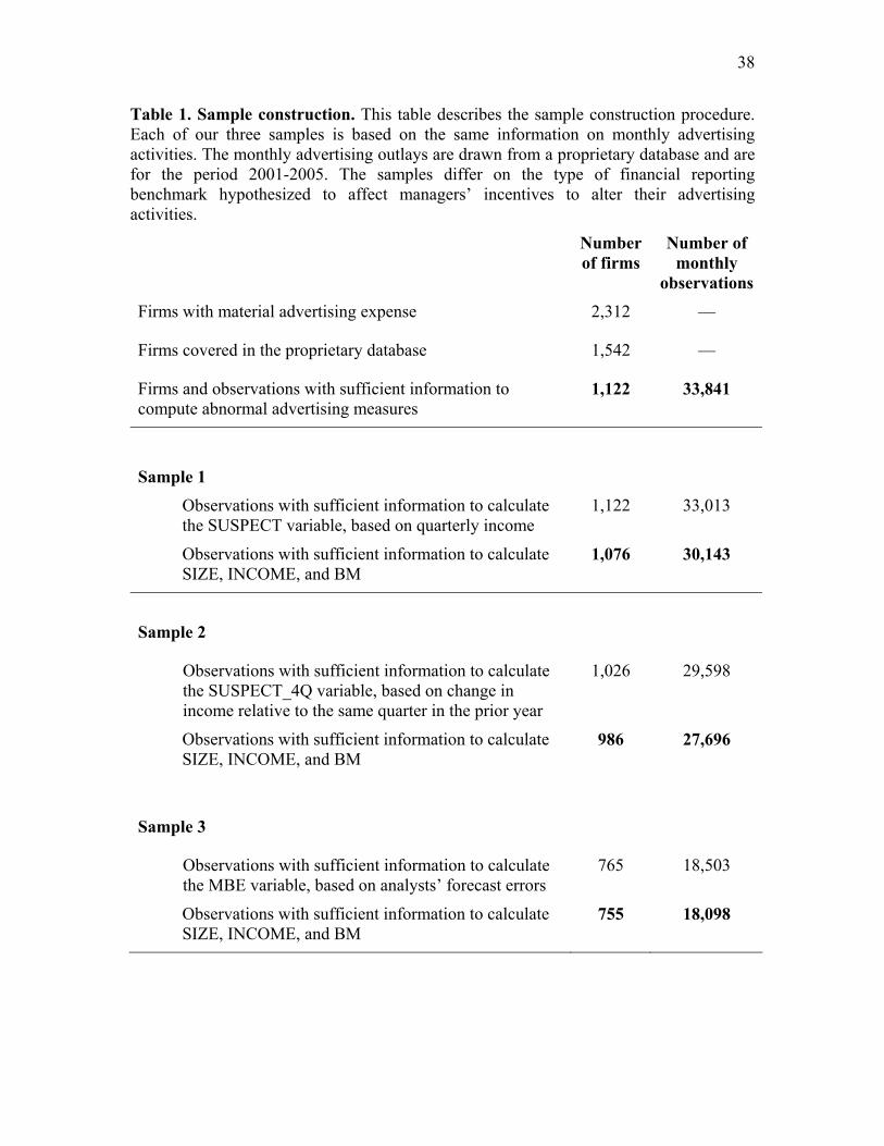
Table 1 reports the steps we took to construct our sample. To make sure that we
include only firms that have substantial advertising budgets, we collect information about
actual advertising activities and media spending information for firms whose average
annual advertising expense over our sample period (2001-2005) exceeds $100,000. We
perform this initial screen using the annual advertising expense figure in Compustat
(data#45). Of those firms (2,312), we identify 1,542 firms that are covered in our
proprietary database.
The main data requirement is the ability to estimate abnormal advertising
activities using the time-series model described in equation (2). This limits our sample to
1,122 firms covering 33,841 monthly observations. Next, we separately construct three
samples based on the variable we use to proxy for financial reporting incentives. As
described in Table 1, after requiring sufficient data on some of the control variables, our
samples cover between 755 and 1,076 firms, and the number of monthly observations
varies from 18,098 to 30,143.
4.3 Summary statistics
Table 2 reports summary statistics for our sample firms. On average, our sample
firms’ revenues are $3.8 billion, with a median of $438 million. As indicated by the
difference between the mean and median, the sample is quite skewed with respect to size.
Similar patterns emerge in total assets (mean of $4.7 billion and median of $435 million)

21
and market capitalization (mean of $5.7 billion and median of $506 million). The average
book-to-market ratio of firms in our sample is 0.76, with a median of 0.42.
The average annual advertising expenses as reported in Compustat (data#45) for
our sample firms is about $100 million, with a median of $9.1 million. Advertising
expenses constitute about 4% of annual sales. Media-related advertising outlays tracked
by the proprietary database we use are $44.5 million, on average, for the same set of
firms. This suggests that media-related outlays constitute about half of advertising
expenses reported in the financial statements. The reason for the difference is that, as
noted earlier, our database tracks only advertising activities related to media spending. It
does not include other forms of advertising such as promotional materials and direct-
response advertising such as catalogs sent to consumers, which are included as part of
the advertising expense in Compustat. The correlation between the annual advertising
expenses reported in Compustat and the annual media-related advertising is 0.85.
5. Results
5.1 Abnormal advertising activities
We first report the results of estimating the time-series model of monthly
advertising outlays as described in equation (2). The purpose of this model is to isolate
the abnormal (discretionary) portion of advertising outlays. One advantage of modeling
advertising outlays as an auto-regressive process is that it does not require a full
specification of all potential determinants of the dependent variable. Instead, it assumes
that the effect of changes in these determinants is captured in the lagged values of the
dependent variable (i.e., advertising outlays), which are used as explanatory variables.
An important feature of our research design is that the high-frequency monthly data we

22
employ in our analyses enable us to estimate a firm-specific auto-regressive time-series
model. Under this approach, the residuals one obtains are less likely to contain
measurement errors that are correlated with omitted variables, unlike the residuals
obtained from industry-based cross-sectional models used in prior studies.
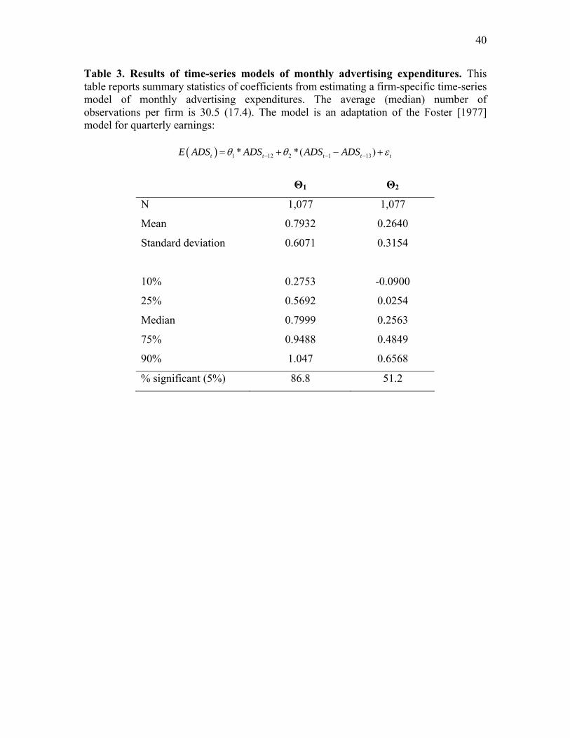
Table 3 reports the estimation results of equation (2). The table reports summary
statistics of the model’s coefficients – θ1 and θ2 – for all 1,076 firm-specific models. The
average number of months used in each firm-specific model is about 30. We observe that
monthly advertising media spending has a strong relation to the media spending in the
same month of the prior year. The average of θ1 is about 0.80, and this coefficient is
statistically significant in over 85% of the firm-specific models. There is also a moving-
average component (θ2), whose coefficient is 0.26 and is significant in over half of the
models.
5.2 Testing the hypotheses
To test our hypotheses of managers’ altering advertising activities to attain their
financial reporting objectives, we estimate variations of the following regression model:
1 2 4_ * * *t tABN ADS INCENTIVE Y INCENTIVE Y Controlsα β β β ε= + + + + + (4)
In equation (4), the dependent variable, ABN_ADSt, is the residual obtained from
firm-specific time-series models of monthly advertising spending described in the
previous section. While this approach tries to minimize the measurement error in our
dependent variable, as discussed in the previous section, it is certainly not free from such
error. However, since this measurement error appears in our dependent variable, its only

23
effect would be manifested in a lower R2. Clearly, this is not likely to bias the inferences
we draw based on the reported results.
INCENTIVE is an indicator variable that is a function of one of three financial
reporting benchmarks: (i) SUSPECT is equal to one if a firm’s quarterly earnings before
extraordinary items (scaled by total assets) are between 0 and 0.00125 (i.e., the bin just to
the right of zero); (ii) SUSPECT_4Q is equal to one if a firm’s quarterly change in
earnings, compared to the same quarter in the previous year, is between 0 and 0.005; and
(iii) MBE is equal to one if a firm just met the consensus analysts’ forecast by one cent;
We interact the main incentive variables with several variables (Y’s) that test our
hypotheses H2-H5. For hypothesis 2, we use an indicator variable (MONTH3) that is
equal to one if the advertising spending occurred during the last month of a fiscal quarter.
For hypothesis 3, we use an indicator variable (QTR4) that is equal to one if the
advertising spending occurred during the fourth fiscal quarter. For hypothesis 4, we use
two continuous variables — the natural logarithm of firm’s age (LNAGE) and the firm’s
net margin (MARGIN). For hypothesis 5, we use an indicator variable (SOX) that is equal
to one if the advertising spending occurred after 2003.
Our control variables include SIZE – the market capitalization of the firm at the
beginning of the fiscal year, INCOME – quarterly earnings before extraordinary items
deflated by beginning of the year’s assets, and BM – the book-to-market ratio at the
beginning of the fiscal year.
Hypotheses 1–3. Tables 4-6 report the results of estimating several versions of
equation (4). The tables vary depending on the financial reporting benchmark that is
being tested. To account for potential dependence among the monthly observations, we

24
calculate the standard errors after clustering observations at the firm level (Petersen
[2007]). Thus, all our statistical tests are based on clustered standard errors.
Beginning with Table 4, where the financial reporting objective is to avoid
reporting a loss (proxied by the SUSPECT variable), we find that in all specifications, the
coefficient on SUSPECT is negative and highly significant (p-values of less than 0.01).
This result is consistent with H1, which suggests that firms manage their advertising
activities to report earnings that just meet the zero earnings benchmark. Moreover, the
negative sign indicates that, on average, suspect firms choose to reduce advertising
activities. Recall that in the case of advertising spending, it is possible that firms would
boost advertising activities in order to increase sales and earnings. However, our results
indicate that, on average, this does not occur. The negative sign on SUSPECT is
consistent with the findings in Roychowdhury [2006], who examines an aggregate
variable of annual discretionary expenses that include research and development, general
and administrative, and advertising expenses.
A few points are worth mentioning. First, our results pertain to actual real
activities taken by managers. This is possible due to the unique feature of our data that
enables us to observe the actual ads that, according to GAAP, are supposed to be
expensed as incurred. Past studies have employed expense-based measures of real
activities, which are also subject to accrual manipulation (for example, aggressive
capitalizations). Therefore, past results could be attributed to both real earnings
management and accrual manipulations. Our advertising spending measures are not
affected by accrual considerations and therefore can be directly attributed to real
activities. Second, we utilize quarterly financial reporting benchmarks that, as reported in

25
Graham, Harvey, and Rajgopal [2005] and Brown and Caylor [2005], are perceived by
managers to be more important than the annual benchmark used in Roychowdhury
[2006]. Third, none of the studies in the literature (Gunny [2005], Roychowdhury [2006],
Zang [2006]) has separately examined advertising activities. As such, our study provides
a finer measure of a single activity as opposed to a coarser measure of multiple activities.
Finally, our high-frequency data provide us with an opportunity for the most powerful
setting for testing our hypotheses.
In addition to reporting the statistical significance of the results, we are also able
to assess the economic significance of the findings pertaining to the SUSPECT variable.
Specifically, the coefficient on SUSPECT indicates that suspect firms reduce their
monthly advertising spending by 0.04% of annual sales, or the quarterly advertising
spending by 0.12% of annual sales. The average annual sales in our sample is $3.8
billion. This means that suspect firms reduce their quarterly advertising outlays by $4.6
million. This reduction constitutes, on average, about 41.5% of quarterly media-related
advertising expenses.
Specification (3) in Table 4 reports the results when we add the MONTH3
variable and the interaction term SUSPECT*MONTH3. The coefficient on MONTH3 is
positive and significant. This means that, on average, firms increase their advertising
outlays in the last month of the fiscal quarter. Examining the interaction term
SUSPECT*MONTH3 sheds light on our second hypothesis. The coefficient on
SUSPECT*MONTH3 is not significant. Thus, we do not find evidence that suspect firms
are more likely to reduce their advertising activities in the third month of a fiscal quarter.
This non-significant result can be interpreted in two alternative ways.

26
First, it is possible that the lag between the decision to cut spending and the actual
reduction in spending is not short enough to enable firms to adjust their advertising
spending in the last month of a fiscal quarter. Recall that firms would like to postpone
cutting spending to a time when information about expected quarterly performance is
more accurate. Thus, any decision to cut advertising activities to meet earning
benchmarks occurs before the third month of the fiscal quarter. This is also consistent
with Zang [2006], who argues that decisions about real activities occur earlier in the
fiscal period, and before any accrual manipulations.
The second interpretation assumes that altering of real activities can only occur
late in the quarter because managers need to learn about the firm’s ongoing performance
in order to know how much to alter real activities. This assumption, of course, is feasible
only in activities that are quick to alter, such as advertising. Under this assumption, the
reduction in quarterly advertising activities is not a response to accounting incentives to
meet certain benchmarks, but rather a reaction to some unobserved changes in economic
conditions. One advantage of our high-frequency setting is that it provides us an
opportunity to explore this alternative interpretation in a powerful way with monthly
data. We believe that our setting is powerful enough to find an effect in the third month,
for two reasons. First, unlike previous studies that pool together several types of
discretionary operating expenses, our focus on a single item increases the likelihood that
our model is well specified. Second, our use of a long firm-specific time-series of
advertising spending further enhances our confidence in the model, which attempts to
separate normal and abnormal advertising activities.

27
The rightmost column in Table 4 reports the results of estimating equation (4)
including the indicator variable QTR4, which equals to one if the observation’s fiscal
quarter is the fourth quarter. In addition, we include the interaction term
SUSPECT*QTR4 to examine whether the general effect of SUSPECT is different during
the fourth quarter. The coefficients on both of these variables are insignificant. This
suggests that the general effect of suspect firms to reduce advertising spending is not
different in the fourth quarter. This result is consistent with firms not using incremental
manipulation of real activities in the fourth quarter because of their lack of ability to alter
these actions late in the fiscal year (Zang [2006]). However, since we believe that
advertising spending is among the real activities with the shortest lag between decision
and execution, our interpretation suggests that the documented reductions, which do not
vary by incentives, may not be due to manipulations of real activities.11
Finally, the only control variable to load significantly is SIZE. Its negative sign
suggests that larger firms are more likely to have lower abnormal advertising activities.
The sign on market capitalization is different than that reported in prior studies (e.g.,
Roychowdhury [2006]. Note, however, that the dependent variable is also different
because it only captures a subset of the expenses measured in Roychowdhury [2006].
Table 5 reports the estimation results of similar models to those reported in Table
4. The difference is that the incentive variable, SUSPECT_4Q, is defined based on the
changes in earnings before extraordinary items relative to the same quarter in the
11 In untabulated results, we assess the impact of changes in real economic conditions on altering discretionary advertising spending by including the percentage change in seasonally adjusted Gross Domestic Products over the previous quarter in our regression models, as an additional explanatory variable. This variable is insignificant, and the variable SUSPECT remains negative and strongly significant. This leads us to conclude that the variable SUSPECT does not merely capture response to changes in economic conditions, at least as they are captured by changes in GDP.

28
previous year. The results in Table 5 are similar to those reported in Table 4. First, the
coefficient on SUSPECT_4Q is consistently negative and significant. Second, there is
weak evidence of higher abnormal advertising spending during the third month of the
fiscal quarter, as the coefficient of MONTH3 is marginally significant (p-value of 0.09).
There is no evidence of incremental abnormal advertising spending by suspect firms
during the third month of the fiscal quarter, as the coefficient on the interaction term
SUSPECT_4Q*MONTH3 is not significantly different from zero. In addition, we do not
find evidence of abnormal advertising spending in the fourth fiscal quarter.
In Table 6, we report results of the third proxy for meeting financial reporting
goals, MBE, which uses analysts’ forecasts as the benchmark. MBE is an indicator
variable that takes the value of one if the firm’s earnings per share for the quarter met the
last outstanding analyst consensus forecast by one cent per share or less. Notice, first, that
the number of observations declines to about 18,000, and the number of firms decreases
to about 760. This reduction is due to additional data requirements imposed by IBES
coverage. The coefficient on the main incentive variable, MBE, is negative in most
specifications, similar to the previous tables. However, the statistical significance of the
evidence is slightly weaker. This could be due to the fact that when trying to meet
analysts’ forecasts, managers do not know exactly what the target should be, as analysts
keep updating their quarterly forecasts throughout the fiscal period. In other words, the
benchmark that managers try to beat is a moving target, and is perhaps harder to achieve
through the manipulation of advertising spending.
As for QTR4, we find that abnormal advertising spending is higher in the fourth
quarter (p-value of 0.009 on QTR4). We also find that the entire significant effect of

29
meeting analysts’ forecasts through advertising spending is attributed to the fourth fiscal
quarter. Notice that MBE turns insignificant while the interaction term MBE*QTR4 is
highly significant. This suggests that with respect to analysts’ forecasts, managers are
able to reduce advertising spending only for the final quarter of the year. This could be
consistent with managers learning throughout the year and, thus, having better
information about analysts’ fourth-quarter forecasts as well as about the firm’s actual
annual financial performance.
Hypothesis 4. Recall that in our fourth hypothesis we raised the possibility that
managers may either decrease or increase advertising activities to achieve certain
earnings benchmarks. This depends on the length of the lead-lag relationship between
advertising activities and their sales response. It also depends on firms’ net margins. In
Table 7, we use two different variables to test this hypothesis. In the first column, we
include the natural log of firms’ age to proxy for the elasticity between advertising and
sales. It is argued that younger firms will tend to have a higher elasticity of advertising-
to-sales than older firms. Therefore, any increase in advertising activities in younger
firms will translate into larger increases in sales than in older firms. We find that older
firms tend to have lower abnormal advertising spending, as reflected in the negative
coefficient on LNAGE. Our main interest lies in the interaction term SUSPECT*LNAGE.
Its coefficient is positive (0.0004) and highly significant. This suggests that older suspect
firms (and not younger) tend to increase advertising activities to avoid reporting losses.
We do not find evidence that such an increase occurs in the third month of the fiscal
period. This result is contrary to the expectation that younger firms will tend to increase
advertising because of the higher elasticity of their advertising activities.
30
The second column in Table 7 examines the association of net margin with the
change in advertising activities. Firms with higher net margins are more likely to increase
sales through increased advertising activities, because any increase in sales will translate
into an increase in earnings, over and above the increase in advertising expenses. We find
no evidence that the general trend suggests an increase in advertising activities for
suspect firms with higher net margins (SUSPECT*MARGIN is insignificant). However,
we find evidence that suspect firms with high margins increase their advertising activities
in the third month of the fiscal quarter. The coefficient on the interaction term
SUSPECT*MARGIN*MONTH3 is positive (0.0258) and significant (p-value of 0.023). In
untabulated results we include both age and margin. The results are similar to those
reported for the separate models.
Hypothesis 5. In our final hypothesis we examine whether there is an increase in
the tendency of managers to engage in real earnings management in the form of altering
advertising activities to meet certain benchmarks following the Sarbanes-Oxley Act.
According to Graham, Harvey, and Rajgopal [2005], managers’ preferences for using
real- versus accrual-based strategies may have changed after the new legislation. Table 8
reports results of our basic model, including an indicator variable, SOX, that equals to one
in the years 2003-2005. The coefficient on SUSPECT*SOX is insignificant. Thus, we find
no evidence of an increased likelihood of using advertising activities to avoid reporting
losses in the post-SOX period.
6. Conclusion
In this paper we study whether managers alter their advertising spending to
achieve financial reporting objectives, such as avoiding reporting a loss, avoiding

31
reporting a decrease in earnings, and meeting analysts’ consensus forecasts. We do so by
utilizing a unique and comprehensive data set of monthly advertising spending in media
outlets. This data set enables us to directly analyze actual real managerial activities that,
according to GAAP, should be expensed as incurred. This is in contrast to examining
reported expenses, which are also subject to accrual manipulations. Therefore, our
approach is different than the one used in prior studies in which reported expenses serve
as an indirect proxy for inferring real earnings management. Our data on advertising
activities also allow us to focus on a specific item that is subject to managerial discretion
as opposed to an aggregate proxy of several discretionary expenses activities. Finally, the
high-frequency feature of our data set provides us with a powerful setting to investigate
the incentives to meet quarterly earnings benchmarks as well as to examine the timing of
real activities’ manipulations.
We find strong evidence that firms reduce their advertising spending in order to
meet all three types of financial reporting objectives we examine. We find weaker
evidence of an increase in abnormal advertising activities in the third month of a fiscal
quarter. However, this increase is not limited to “suspect” firms, i.e., firms that have just
achieved the three financial reporting objectives. One exception is that we do find
evidence of increased advertising activities to meet analysts’ forecasts during the third
month of the fiscal quarter. Finally, we uncover circumstances in which firms have
incentives to increase advertising spending to avoid reporting a loss. Specifically, firms
with higher net margins are associated with higher abnormal advertising spending in the
third month of the fiscal quarter.

32
Overall, this study contributes to the emerging literature on real earnings
management activities. The evidence we provide enhances our understanding of the
interplay between managers’ incentives and the real actions managers take to achieve
financial reporting goals.

33
References
Accounting Principles Board. Interim Financial Reporting. APB Opinion No. 28. New York, 1973.
Arora, R. “How Promotion Elasticities Change.” Journal of Advertising Research 19(3) (1979): 57–62.
Assmus, G.; J. Farley; and D. R. Lehmann. “How Advertising Affects Sales: Meta-analysis of Econometric Results.” Journal of Marketing Research, 21(1) (1984): 65–74.
Brown, L., and M. Caylor. “A Temporal Analysis of Quarterly Earnings Thresholds: Propensities and Valuation Consequences.” The Accounting Review 80(2) (2005): 423–40.
Bruns, W., and K. Merchant. “The Dangerous Morality of Managing Earnings.” Management Accounting 72(2) (1990): 22–5.
Burgstahler, D., and I. Dichev. “Earnings Management to Avoid Earnings Decreases and Losses.” Journal of Accounting and Economics 24(1) (1997): 99–126.
Cohen, D.; A. Dey; and T. Lys. “The Sarbanes Oxley Act of 2002: Implications for Compensation Structure and Risk-taking Incentives of CEOs.” Working paper, New York University, 2005.
Cohen, D.; A. Dey; and T. Lys. “Real and Accrual Based Earnings Management in the Pre and Post Sarbanes Oxley Periods.” Working paper, New York University, 2007.
Darrough, M., and S. Rangan. “Do Insiders Manipulate Earnings When They Sell Their Shares in an Initial Public Offering?” Journal of Accounting Research 45 (2005): 1–33.
DeGeorge, F.; J. Patell; and R. Zeckhauser. “Earnings Management to Exceed Thresholds.” Journal of Business 72 (1979): 1–33.
Deighton, J.; C. Henderson; and S. Neslin. “The Effects of Advertising on Brand Switching and Repeat Purchasing.” Journal of Marketing Research 31(1) (1994): 28–43.
Fields, T. D.; T. Z. Lys; and L. Vincent. “Empirical Research on Accounting Choice.” Journal of Accounting and Economics 31 (2001): 255–307.
Financial Accounting Standards Board (FASB). Reporting Accounting Changes in Interim Financial Statements. Statement of Financial Accounting Standards No. 3. Stamford, CT, 1974.
Financial Accounting Standards Board (FASB). FASB Interpretation No. 18. Accounting

34
for Income Taxes in Interim Periods. Stamford, CT, 1977.
Foster, G. “Quarterly Accounting Data: Time-Series Properties and Predictive Ability Results.” The Accounting Review 52 (1977): 1–21.
Graham, J. R.; C. R. Harvey; and S. Rajgopal. “The Economic Implications of Corporate Financial Reporting.” Journal of Accounting and Economics 40 (2005): 3–73.
Gunny, K. “What Are the Consequences of Real Earnings Management?” Working paper, University of Colorado, 2005.
Healy, P., and J. Wahlen. “A Review of the Earnings Management Literature and Its Implications for Standard Setting.” Accounting Horizons 13 (1999): 365–84.
Jones, J. “Exposure Effects Under a Microscope.” Admap, 30 (February) (1995): 28–31.
Kothari, S. P. “Capital Market Research in Accounting.” Journal of Accounting and Economics 31 (2001): 105–231.
McDonald, C. “What Is the Short Term Effect of Advertising?” In Measuring the Effect of Advertising, D. Corkindale and S. Kennedy, eds. Farnborough, England: Saxon House Studies, 1971: 463–87.
McNichols, M. Discussion of “Why Are Earnings Kinky? An Examination of the Earnings Management Explanation.” Review of Accounting Studies 8 (2003), 385–91.
Parker, P. M., and H. Gatignon. “Order of Entry, Trial Diffusion, and Elasticity Dynamics: An Empirical Case.” Marketing Letters 7(1) (1996): 95–109.
Parsons, L. “The Product Life Cycle and Time-Varying Advertising Elasticities.” Journal of Marketing Research 12 (November) (1975): 476–80.
Petersen, M. “Estimating Standard Errors in Finance Panel Data Sets: Comparing Approaches.” Review of Financial Studies, Forthcoming, 2007.
Rogers, W. “Regression Standard Errors in Clustered Samples.” Stata Technical Bulletin 13 (1993):19–23.
Roychowdhury, S. “Earnings Management through Real Activities Manipulation.” Journal of Accounting and Economics 42 (2006): 335–70.
Winer, R. S. “An Analysis of the Time-Varying Effects of Advertising: The Case of Lydia Pinkham.” Journal of Business 52(4) (1979): 563–76.
Zang, A. “Evidence on the Tradeoff between Real Manipulation and Accrual Manipulation.” Working paper, University of Rochester, 2006.

35
Appendix A Our database records advertising activities at the time they appear in a media outlet (e.g., when they are aired on television or appear in print). According to Statement of Position (SOP) 93-7: Reporting on Advertising Costs, firms are required to expense advertising activities as they are incurred. Thus, if firms follow GAAP, our database will include all media-related advertising that should have been expensed in the period in which they were aired or printed.
The following paragraphs from SOP 93-7 describe the accounting treatment in detail:
Paragraph 26
The costs of advertising should be expensed either as incurred or the first time the advertising takes place… except for-- a. Direct-response advertising (1) whose primary purpose is to elicit sales to
customers who could be shown to have responded specifically to the advertising and (2) that results in probable future economic benefits.
b. Expenditures for advertising costs that are made subsequent to recognizing revenues related to those costs
Paragraph 42
Advertising activities may have several component costs. Two primary components, which are made up of other components, are the costs of (a) producing advertisements, such as the costs of idea development, writing advertising copy, artwork, printing, audio and video crews, actors, and other costs, and (b) communicating advertisements that have been produced, such as the costs of magazine space, television airtime, billboard space, and distribution (postage stamps, for example).
Paragraph 43
Costs of producing advertising are incurred during production rather than when the advertising takes place.
Paragraph 44
Costs of communicating advertising are not incurred until the item or service has been received and should not be reported as expenses before the item or service has been received… For example--
• The costs of television airtime should not be reported as advertising expense before the airtime is used. Once it is used, the costs should be expensed, unless the airtime was used for direct-response advertising activities that meet the criteria for capitalization under this SOP.
• The costs of magazine, directory, or other print media advertising space should not be reported as advertising expense before the space is used. Once it is used,

36
the costs should be expensed, unless the space was used for direct-response advertising activities that meet the criteria for capitalization under this SOP.
Our database contains only media-related advertising that cannot be treated as direct-response advertising and therefore has to be expensed in the period of appearance.
Suppose that an advertisement appeared on television on January 15, 2007. This advertisement will be captured in our database. If the firm follows GAAP, the advertisement will appear as an expense in the financial statements for the quarter ending on March 31, 2007. Thus, our database captures all media-related advertising activities during the period that are supposed to be expensed in the income statement.

37
Appendix B This appendix describes the various media outlets from which the advertising data are collected.
1. Television
Cable Television: Commercial occurrences and advertising activities information for 52 cable television networks. Cable television is monitored via satellite 24 hours a day, 365 days a year.
Spot Television: Commercial occurrence and expenditure information for more than 600 English-speaking stations and 35 Spanish-speaking stations in 100 major markets. Spot television is monitored 21 hours a day (5 a.m. to 2 a.m.). The monitored stations constitute the principal stations in each market and typically include the network affiliates, major independents, and Spanish affiliates. Public broadcasting stations are not monitored.
Network Television: Commercial occurrence and expenditure information for seven broadcast networks: ABC, CBS, FOX, NBC, PAX/I, MNTV, and CW.
2. Print
Magazines: All paid advertising space and expenditure data in over 350 consumer magazines and over 30 local magazines.
Newspapers: All advertising space in over 250 daily and Sunday newspaper editions and Sunday magazines, including national newspapers such as The New York Times, USA Today, and Wall Street Journal. In national newspapers, all national and regional editions are measured.
3. Radio
Local Radio: Data are based on the tracking of radio billings by stations in more than 100 radio markets.
National Spot Radio: Nationally placed spot radio data for approximately 4,000 stations in more than 225 markets. Reported expenditures are based on audited billings from contract information provided by the following major national station representative organizations: ABC, Allied, Christal, Clear Channel, Cumulus, D&R, Infinity, Katz, KHM, Lotus, and McGavren.
4. Internet
Advertising expenditure information is measured for over 2,500 sites and 90,000 brands in the United States and Canada. A proprietary spider probes the sites on an ongoing basis and captures and stores every image on a page.
38
Table 1. Sample construction. This table describes the sample construction procedure. Each of our three samples is based on the same information on monthly advertising activities. The monthly advertising outlays are drawn from a proprietary database and are for the period 2001-2005. The samples differ on the type of financial reporting benchmark hypothesized to affect managers’ incentives to alter their advertising activities.
Number of firms
Number of monthly
observations Firms with material advertising expense 2,312 —
Firms covered in the proprietary database 1,542 —
Firms and observations with sufficient information to compute abnormal advertising measures
1,122 33,841
Sample 1
Observations with sufficient information to calculate the SUSPECT variable, based on quarterly income
1,122 33,013
Observations with sufficient information to calculate SIZE, INCOME, and BM
1,076 30,143
Sample 2
Observations with sufficient information to calculate the SUSPECT_4Q variable, based on change in income relative to the same quarter in the prior year
1,026 29,598
Observations with sufficient information to calculate SIZE, INCOME, and BM
986 27,696
Sample 3
Observations with sufficient information to calculate the MBE variable, based on analysts’ forecast errors
765 18,503
Observations with sufficient information to calculate SIZE, INCOME, and BM
755 18,098

39
Table 2. Descriptive statistics for sample firms. This table reports summary statistics for our final sample of 1,076 firms. The numbers reported are the summary of the firm-average across the five sample years. Sales is defined as the annual figure of total sales in million of dollars from Compustat (data#12). Assets is defined as total assets from Compustat (data#6). BM is the book-to-market ratio. Advertising expenses is the annual advertising expense from Compustat (data#45). Advertising outlays is the annual sum of all monthly media-related advertising outlays tracked by our proprietary database. Mean Median Std 25% 75%
Sales (Mil $) 3,848 438.3 14,569 118.3 1,654.1
Assets (Mil $) 4,743 435.2 21,314 122.4 1,699
Market capitalization (Mil $) 5,695 506.2 22,902 136.0 2,034.3
BM 0.76 0.42 4.01 0.24 0.70
Advertising expenses (Mil $) 100.2 9.1 360.6 1.7 42.2
Ad expenses/Sales 4.03% 1.94% 8.06% 0.88% 4.61%
Advertising outlays (Mil $) 44.5 1.76 187.3 0.25 13.1
Ad outlays/Sales 2.35% 0.49% 8.95% 0.11% 1.81%
40
Table 3. Results of time-series models of monthly advertising expenditures. This table reports summary statistics of coefficients from estimating a firm-specific time-series model of monthly advertising expenditures. The average (median) number of observations per firm is 30.5 (17.4). The model is an adaptation of the Foster [1977] model for quarterly earnings:
( ) 1 12 2 1 13* *( )t t t t tE ADS ADS ADS ADSθ θ ε− − −= + − +
Θ1 Θ2
N 1,077 1,077
Mean 0.7932 0.2640
Standard deviation 0.6071 0.3154
10% 0.2753 -0.0900
25% 0.5692 0.0254
Median 0.7999 0.2563
75% 0.9488 0.4849
90% 1.047 0.6568
% significant (5%) 86.8 51.2

41
Table 4. Tests of real earnings management based on monthly advertising activities. The table reports estimation results of models whose dependent variable is monthly abnormal advertising expenditures. These are calculated based on the residuals from firm-specific time-series models estimated up to 60 months (an average of 30 months). SUSPECT is an indicator variable equal to one if quarterly income before extraordinary items deflated by total assets is above 0 and less than 0.0125%. MONTH3 is an indicator variable equal to one if the month is the third month of a fiscal quarter. QTR4 is an indicator variable equal to one if the quarter is the fourth fiscal quarter. INCOME is income before extraordinary items deflated by total assets at the beginning of the year; BM is the book-to-market ratio. SIZE is the natural logarithm of market capitalization. P-values in parentheses are based on robust firm-clustered standard errors (e.g., Rogers [1993], Petersen [2007]). ***, **, and * indicate significance at 1%, 5%, and 10% levels. (1) (2) (3) (4)
INTERCEPT 0.0004 0.0014 0.0013 0.0014 (0.000)*** (0.001)*** (0.001)*** (0.001)***
SUSPECT -0.0003 -0.0004 -0.0004 -0.0004 (0.000)*** (0.001)*** (0.001)*** (0.001)***
MONTH3 0.0001 (0.021)**
SUSPECT*MONTH3 -0.0001 (0.890)
QTR4 0.0001 (0.417)
SUSPECT*QTR4 0.0001 (0.591)
SIZE -0.0001 -0.0001 -0.0001 (0.009)*** (0.009)*** (0.009)***
INCOME -0.007 -0.0071 -0.0071 (0.124) (0.124) (0.124)
BM -0.0001 -0.0001 -0.0001 (0.291) (0.291) (0.292)
Observations 33,013 30,143 30,143 30,143
Adjusted R-squared 0.0000 0.0048 0.0048 0.0048
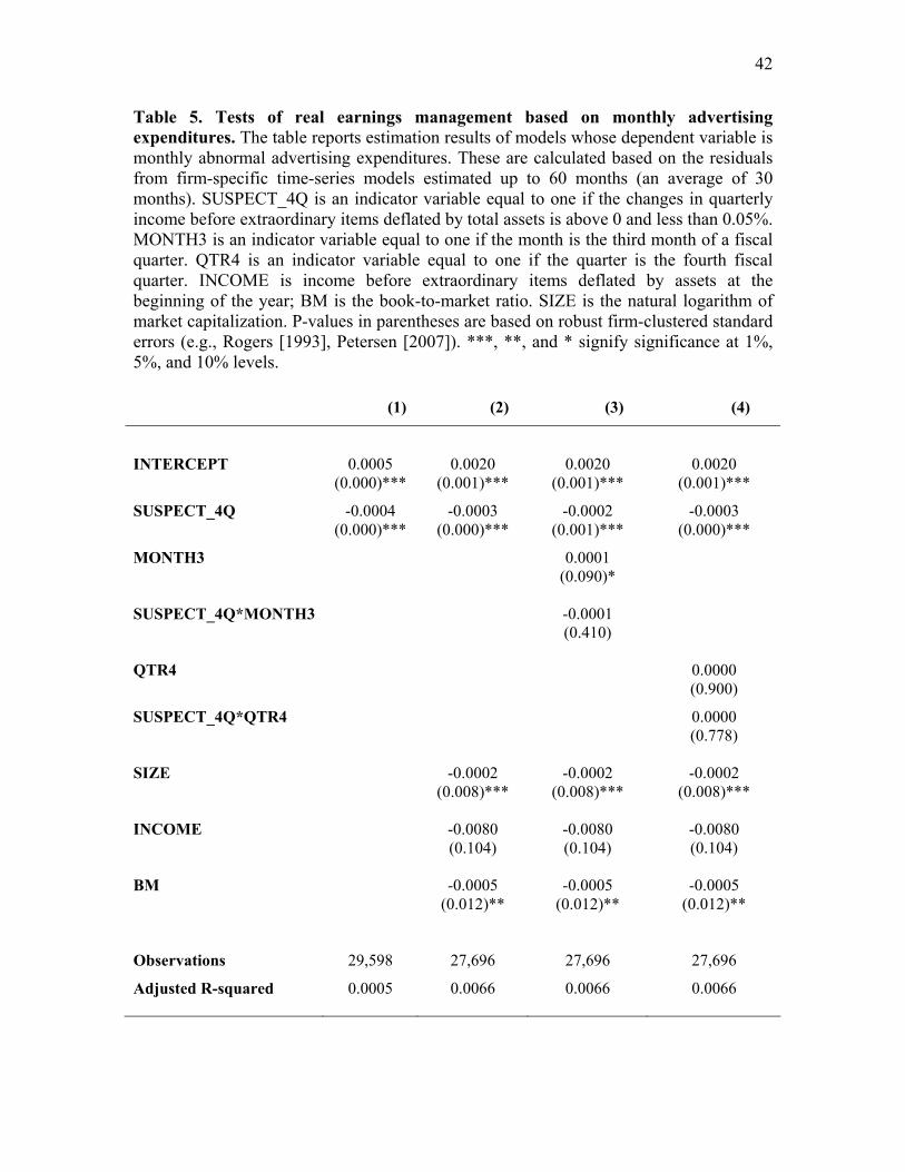
42
Table 5. Tests of real earnings management based on monthly advertising expenditures. The table reports estimation results of models whose dependent variable is monthly abnormal advertising expenditures. These are calculated based on the residuals from firm-specific time-series models estimated up to 60 months (an average of 30 months). SUSPECT_4Q is an indicator variable equal to one if the changes in quarterly income before extraordinary items deflated by total assets is above 0 and less than 0.05%. MONTH3 is an indicator variable equal to one if the month is the third month of a fiscal quarter. QTR4 is an indicator variable equal to one if the quarter is the fourth fiscal quarter. INCOME is income before extraordinary items deflated by assets at the beginning of the year; BM is the book-to-market ratio. SIZE is the natural logarithm of market capitalization. P-values in parentheses are based on robust firm-clustered standard errors (e.g., Rogers [1993], Petersen [2007]). ***, **, and * signify significance at 1%, 5%, and 10% levels.
(1) (2) (3) (4)
INTERCEPT 0.0005 0.0020 0.0020 0.0020 (0.000)*** (0.001)*** (0.001)*** (0.001)***
SUSPECT_4Q -0.0004 -0.0003 -0.0002 -0.0003 (0.000)*** (0.000)*** (0.001)*** (0.000)***
MONTH3 0.0001 (0.090)*
SUSPECT_4Q*MONTH3 -0.0001 (0.410)
QTR4 0.0000 (0.900)
SUSPECT_4Q*QTR4 0.0000 (0.778)
SIZE -0.0002 -0.0002 -0.0002 (0.008)*** (0.008)*** (0.008)***
INCOME -0.0080 -0.0080 -0.0080 (0.104) (0.104) (0.104)
BM -0.0005 -0.0005 -0.0005 (0.012)** (0.012)** (0.012)**
Observations 29,598 27,696 27,696 27,696
Adjusted R-squared 0.0005 0.0066 0.0066 0.0066
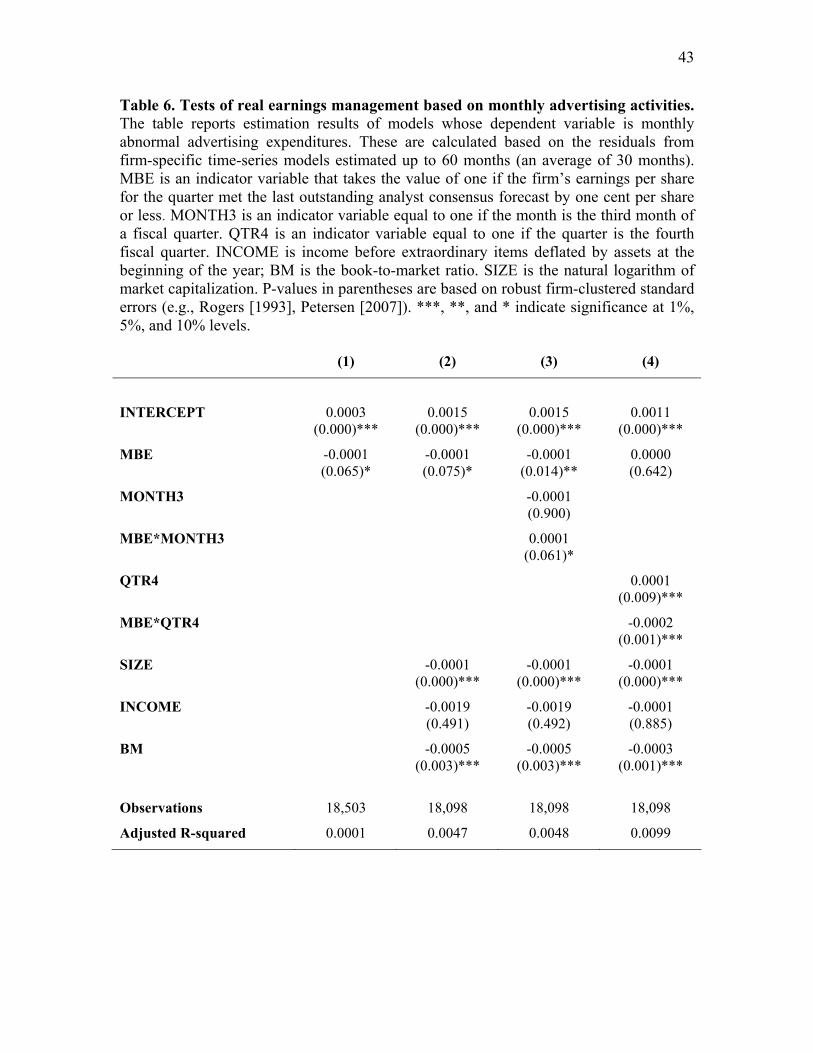
43
Table 6. Tests of real earnings management based on monthly advertising activities. The table reports estimation results of models whose dependent variable is monthly abnormal advertising expenditures. These are calculated based on the residuals from firm-specific time-series models estimated up to 60 months (an average of 30 months). MBE is an indicator variable that takes the value of one if the firm’s earnings per share for the quarter met the last outstanding analyst consensus forecast by one cent per share or less. MONTH3 is an indicator variable equal to one if the month is the third month of a fiscal quarter. QTR4 is an indicator variable equal to one if the quarter is the fourth fiscal quarter. INCOME is income before extraordinary items deflated by assets at the beginning of the year; BM is the book-to-market ratio. SIZE is the natural logarithm of market capitalization. P-values in parentheses are based on robust firm-clustered standard errors (e.g., Rogers [1993], Petersen [2007]). ***, **, and * indicate significance at 1%, 5%, and 10% levels. (1) (2) (3) (4)
INTERCEPT 0.0003 0.0015 0.0015 0.0011 (0.000)*** (0.000)*** (0.000)*** (0.000)***
MBE -0.0001 -0.0001 -0.0001 0.0000 (0.065)* (0.075)* (0.014)** (0.642)
MONTH3 -0.0001 (0.900)
MBE*MONTH3 0.0001 (0.061)*
QTR4 0.0001 (0.009)***
MBE*QTR4 -0.0002 (0.001)***
SIZE -0.0001 -0.0001 -0.0001 (0.000)*** (0.000)*** (0.000)***
INCOME -0.0019 -0.0019 -0.0001 (0.491) (0.492) (0.885)
BM -0.0005 -0.0005 -0.0003 (0.003)*** (0.003)*** (0.001)***
Observations 18,503 18,098 18,098 18,098
Adjusted R-squared 0.0001 0.0047 0.0048 0.0099

44
Table 7. Tests of real earnings management based on monthly advertising expenditures. The table reports estimation results of models whose dependent variable is monthly abnormal advertising expenditures. These are calculated based on the residuals from firm-specific time-series models estimated up to 60 months (an average of 30 months). The analysis is conducted on a limited number of observations that are closest to the area of zero earnings. Specifically, we use observations whose earnings before extraordinary items deflated by total assets is between -0.0075 and 0.00625. SUSPECT is an indicator variable equal to one if quarterly income before extraordinary items deflated by total assets is above 0 and less than 0.0125%. MONTH3 is an indicator variable equal to one if the month is the third month of a fiscal quarter. QTR4 is an indicator variable equal to one if the quarter is the fourth fiscal quarter. INCOME is income before extraordinary items deflated by assets at the beginning of the year; BM is the book-to-market ratio. SIZE is the natural logarithm of market capitalization. P-values in parentheses are based on robust firm-clustered standard errors (e.g., Rogers [1993], Petersen [2007]). ***, **, and * signify significance at 1%, 5%, and 10% levels.
X= LNAGE
X= MARGIN
INTERCEPT 0.0019 (0.000)***
0.0013 (0.001)***
SUSPECT -0.0014 (0.002)***
-0.0004 (0.006)***
MONTH3 0.0001 (0.022)***
0.0001 (0.018)***
SUSPECT*MONTH3 -0.0002 (0.700)
-0.0001 (0.296)
X -0.0003 (0.001)***
-0.0001 (0.427)
SUSPECT*X 0.0004 (0.010)***
-0.0068 (0.641)
SUSPECT* X* MONTH3 0.0001 (0.733)
0.0258 (0.023)***
SIZE -0.0001 (0.060)**
-0.0001 (0.011)**
INCOME -0.0073 (0.118)
-0.0066 (0.124)
BM -0.0001 (0.349)
-0.0001 (0.291)
Observations 29,561 30,124 Adjusted R-squared 0.0060 0.0054

45
Table 8. Tests of real earnings management based on monthly advertising expenditures following SOX. The table reports estimation results of models whose dependent variable is monthly abnormal advertising expenditures. These are calculated based on the residuals from firm-specific time-series models estimated up to 60 months (an average of 30 months). SUSPECT is an indicator variable equal to one if quarterly income before extraordinary items deflated by total assets is above 0 and less than 0.0125%. SOX is an indicator variable taking the value of one if the observation is in 2003 and onward and 0 otherwise. INCOME is income before extraordinary items deflated by assets at the beginning of the year; BM is the book-to-market ratio. SIZE is the natural logarithm of market capitalization. P-values in parentheses are based on robust firm-clustered standard errors (e.g., Rogers [1993], Petersen [2007]). ***, **, and * signify significance at 1%, 5%, and 10% levels.
INTERCEPT 0.0014 (0.001)***
SUSPECT -0.0004 (0.029)**
SOX -0.0001 (0.539)
SOX*SUSPECT -0.0000 (0.890)
SIZE -0.0001 (0.010)***
INCOME -0.0071 (0.124)
BM -0.0001 (0.293)
Observations 30,143 Adjusted R-squared 0.0048