the unreasonable effectiveness of random projections in ...axk/hdm_bobdurrant.pdf · we call the k...
TRANSCRIPT
The Unreasonable Effectiveness of RandomProjections in Computer Science
Robert J. Durrant
University of Waikato,Department of Statistics
www.stats.waikato.ac.nz/˜bobd
2nd IEEE ICDM Workshop on High Dimensional Data Mining,Sunday 14th December 2014
R.J.Durrant (U.Waikato) Unreasonable Effectiveness of RP in CS HDM 2014 1 / 113

Outline1 Background and Preliminaries
2 Johnson-Lindenstrauss Lemma (JLL) and extensions
3 Applications of JLL (1)Approximate Nearest Neighbour SearchRP PerceptronMixtures of Gaussians
4 Compressed SensingSVM from RP sparse data
5 Applications of JLL (2)RP LLS Regression
6 JLL- and CS-free ApproachesRP Fisher’s Linear Discriminant
Time Complexity AnalysisExperiments
RP Estimation of Distribution Algorithm
R.J.Durrant (U.Waikato) Unreasonable Effectiveness of RP in CS HDM 2014 2 / 113

Outline
1 Background and Preliminaries
2 Johnson-Lindenstrauss Lemma (JLL) and extensions
3 Applications of JLL (1)
4 Compressed Sensing
5 Applications of JLL (2)
6 JLL- and CS-free Approaches
R.J.Durrant (U.Waikato) Unreasonable Effectiveness of RP in CS HDM 2014 3 / 113

Motivation - Dimensionality Curse
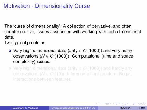
The ‘curse of dimensionality’: A collection of pervasive, and oftencounterintuitive, issues associated with working with high-dimensionaldata.Two typical problems:
Very high dimensional data (arity ∈ O (1000)) and very manyobservations (N ∈ O (1000)): Computational (time and spacecomplexity) issues.Very high dimensional data (arity ∈ O (1000)) and hardly anyobservations (N ∈ O (10)): Inference a hard problem. Bogusinteractions between features.
R.J.Durrant (U.Waikato) Unreasonable Effectiveness of RP in CS HDM 2014 4 / 113
Motivation - Dimensionality Curse
The ‘curse of dimensionality’: A collection of pervasive, and oftencounterintuitive, issues associated with working with high-dimensionaldata.Two typical problems:
Very high dimensional data (arity ∈ O (1000)) and very manyobservations (N ∈ O (1000)): Computational (time and spacecomplexity) issues.Very high dimensional data (arity ∈ O (1000)) and hardly anyobservations (N ∈ O (10)): Inference a hard problem. Bogusinteractions between features.
R.J.Durrant (U.Waikato) Unreasonable Effectiveness of RP in CS HDM 2014 4 / 113

Curse of Dimensionality
Comment:What constitutes high-dimensional depends on the problem setting,but data vectors with arity in the thousands very common in practice(e.g. medical images, gene activation arrays, text, time series, ...).
Issues can start to show up when data arity in the tens!
We will simply say that the observations, T , are d-dimensional andthere are N of them: T = xi ∈ RdNi=1 and we will assume that, forwhatever reason, d is too large.
R.J.Durrant (U.Waikato) Unreasonable Effectiveness of RP in CS HDM 2014 5 / 113
Mitigating the Curse of Dimensionality
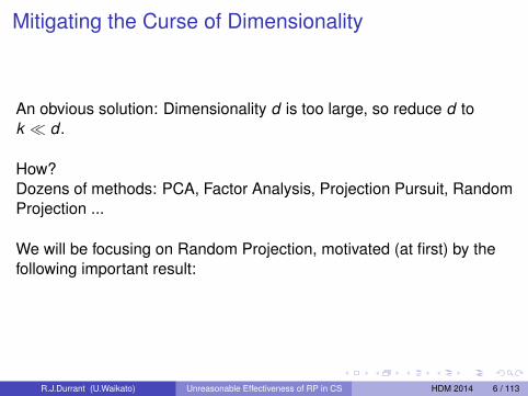
An obvious solution: Dimensionality d is too large, so reduce d tok d .
How?Dozens of methods: PCA, Factor Analysis, Projection Pursuit, RandomProjection ...
We will be focusing on Random Projection, motivated (at first) by thefollowing important result:
R.J.Durrant (U.Waikato) Unreasonable Effectiveness of RP in CS HDM 2014 6 / 113

Outline
1 Background and Preliminaries
2 Johnson-Lindenstrauss Lemma (JLL) and extensions
3 Applications of JLL (1)
4 Compressed Sensing
5 Applications of JLL (2)
6 JLL- and CS-free Approaches
R.J.Durrant (U.Waikato) Unreasonable Effectiveness of RP in CS HDM 2014 7 / 113

Johnson-Lindenstrauss Lemma (JLL)The JLL is the following rather surprising fact:
Theorem (Johnson and Lindenstrauss, 1984)
Let ε ∈ (0,1). Let N, k ∈ N with V ⊆ Rd a set of N points andk ∈ O
(mind , ε−2 log N
). Then there exists a mapping P : Rd → Rk ,
such that for all u, v ∈ V:
(1− ε)‖u − v‖2d 6 ‖Pu − Pv‖2k 6 (1 + ε)‖u − v‖2d
Dot products are also approximately preserved by P since if JLLholds then: uT v − ε 6 (Pu)T Pv 6 uT v + ε. (Proof: parallelogramlaw).Note that the projection dimension k depends only on ε and N.For linear mappings scale of k is sharp: No linear dimensionalityreduction can improve on JLL guarantee for an arbitrary point set.Lower bound k ∈ Ω
(mind , ε−2 log N
)[LN14].
R.J.Durrant (U.Waikato) Unreasonable Effectiveness of RP in CS HDM 2014 8 / 113

Distributional JLL
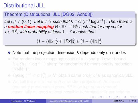
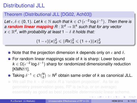
Theorem (Distributional JLL [DG02, Ach03])
Let ε, δ ∈ (0,1). Let k ∈ N such that k ∈ O(ε−2 log δ−1). Then there is
a random linear mapping R : Rd → Rk such that for any vectorx ∈ Rd , with probability at least 1− δ it holds that:
(1− ε)‖x‖2d 6 ‖Rx‖2k 6 (1 + ε)‖x‖2d
Note that the projection dimension k depends only on ε and δ.For random linear mappings scale of k is sharp: Lower boundk ∈ Ω(ε−2 log δ−1) sharp for randomized dimensionality reduction[KMN11].Taking δ−1 ∈ O
(N2
)' N2 obtain same order of k as canonical JLL.
We call the k × d matrix R a ‘random projection’. As far asgeometry preservation goes, RP is (w.h.p, or on average)essentially as good as best possible deterministic linear scheme.
R.J.Durrant (U.Waikato) Unreasonable Effectiveness of RP in CS HDM 2014 9 / 113
Distributional JLL
Theorem (Distributional JLL [DG02, Ach03])
Let ε, δ ∈ (0,1). Let k ∈ N such that k ∈ O(ε−2 log δ−1). Then there is
a random linear mapping R : Rd → Rk such that for any vectorx ∈ Rd , with probability at least 1− δ it holds that:
(1− ε)‖x‖2d 6 ‖Rx‖2k 6 (1 + ε)‖x‖2d
Note that the projection dimension k depends only on ε and δ.For random linear mappings scale of k is sharp: Lower boundk ∈ Ω(ε−2 log δ−1) sharp for randomized dimensionality reduction[KMN11].Taking δ−1 ∈ O
(N2
)' N2 obtain same order of k as canonical JLL.
We call the k × d matrix R a ‘random projection’. As far asgeometry preservation goes, RP is (w.h.p, or on average)essentially as good as best possible deterministic linear scheme.
R.J.Durrant (U.Waikato) Unreasonable Effectiveness of RP in CS HDM 2014 9 / 113
Intuition
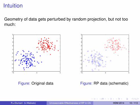
Geometry of data gets perturbed by random projection, but not toomuch:
−5 0 5−5
−4
−3
−2
−1
0
1
2
3
4
5
Figure: Original data
−5 0 5−5
−4
−3
−2
−1
0
1
2
3
4
5
Figure: RP data (schematic)
R.J.Durrant (U.Waikato) Unreasonable Effectiveness of RP in CS HDM 2014 10 / 113

Intuition
Geometry of data gets perturbed by random projection, but not toomuch:
−5 0 5−5
−4
−3
−2
−1
0
1
2
3
4
5
Figure: Original data
−5 0 5−5
−4
−3
−2
−1
0
1
2
3
4
5
Figure: RP data & Original data
R.J.Durrant (U.Waikato) Unreasonable Effectiveness of RP in CS HDM 2014 11 / 113

Applications
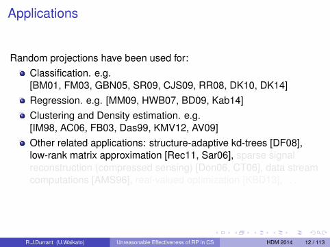
Random projections have been used for:Classification. e.g.[BM01, FM03, GBN05, SR09, CJS09, RR08, DK10, DK14]Regression. e.g. [MM09, HWB07, BD09, Kab14]Clustering and Density estimation. e.g.[IM98, AC06, FB03, Das99, KMV12, AV09]Other related applications: structure-adaptive kd-trees [DF08],low-rank matrix approximation [Rec11, Sar06], sparse signalreconstruction (compressed sensing) [Don06, CT06], data streamcomputations [AMS96], real-valued optimization [KBD13], . . .
R.J.Durrant (U.Waikato) Unreasonable Effectiveness of RP in CS HDM 2014 12 / 113

Applications
Random projections have been used for:Classification. e.g.[BM01, FM03, GBN05, SR09, CJS09, RR08, DK10, DK14]Regression. e.g. [MM09, HWB07, BD09, Kab14]Clustering and Density estimation. e.g.[IM98, AC06, FB03, Das99, KMV12, AV09]Other related applications: structure-adaptive kd-trees [DF08],low-rank matrix approximation [Rec11, Sar06], sparse signalreconstruction (compressed sensing) [Don06, CT06], data streamcomputations [AMS96], real-valued optimization [KBD13], . . .
R.J.Durrant (U.Waikato) Unreasonable Effectiveness of RP in CS HDM 2014 12 / 113

Distributional JLL - Proof Ideas
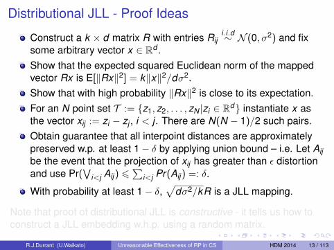
Construct a k × d matrix R with entries Riji.i.d∼ N (0, σ2) and fix
some arbitrary vector x ∈ Rd .Show that the expected squared Euclidean norm of the mappedvector Rx is E[‖Rx‖2] = k‖x‖2/dσ2.Show that with high probability ‖Rx‖2 is close to its expectation.For an N point set T := z1, z2, . . . , zN |zi ∈ Rd instantiate x asthe vector xij := zi − zj , i < j . There are N(N − 1)/2 such pairs.Obtain guarantee that all interpoint distances are approximatelypreserved w.p. at least 1− δ by applying union bound – i.e. Let Aijbe the event that the projection of xij has greater than ε distortionand use Pr(
∨i<j Aij) 6
∑i<j Pr(Aij) =: δ.
With probability at least 1− δ,√
dσ2/kR is a JLL mapping.
Note that proof of distributional JLL is constructive - it tells us how toconstruct a JLL embedding w.h.p. using a random matrix.
R.J.Durrant (U.Waikato) Unreasonable Effectiveness of RP in CS HDM 2014 13 / 113

Distributional JLL - Proof Ideas
Construct a k × d matrix R with entries Riji.i.d∼ N (0, σ2) and fix
some arbitrary vector x ∈ Rd .Show that the expected squared Euclidean norm of the mappedvector Rx is E[‖Rx‖2] = k‖x‖2/dσ2.Show that with high probability ‖Rx‖2 is close to its expectation.For an N point set T := z1, z2, . . . , zN |zi ∈ Rd instantiate x asthe vector xij := zi − zj , i < j . There are N(N − 1)/2 such pairs.Obtain guarantee that all interpoint distances are approximatelypreserved w.p. at least 1− δ by applying union bound – i.e. Let Aijbe the event that the projection of xij has greater than ε distortionand use Pr(
∨i<j Aij) 6
∑i<j Pr(Aij) =: δ.
With probability at least 1− δ,√
dσ2/kR is a JLL mapping.
Note that proof of distributional JLL is constructive - it tells us how toconstruct a JLL embedding w.h.p. using a random matrix.
R.J.Durrant (U.Waikato) Unreasonable Effectiveness of RP in CS HDM 2014 13 / 113

What is Random Projection? (1)
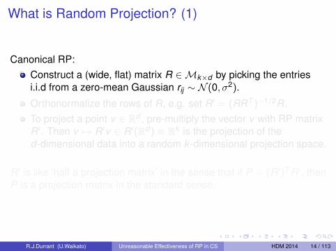
Canonical RP:Construct a (wide, flat) matrix R ∈Mk×d by picking the entriesi.i.d from a zero-mean Gaussian rij ∼ N (0, σ2).
Orthonormalize the rows of R, e.g. set R′ = (RRT )−1/2R.To project a point v ∈ Rd , pre-multiply the vector v with RP matrixR′. Then v 7→ R′v ∈ R′(Rd ) ≡ Rk is the projection of thed-dimensional data into a random k -dimensional projection space.
R′ is like ‘half a projection matrix’ in the sense that if P = (R′)T R′, thenP is a projection matrix in the standard sense.
R.J.Durrant (U.Waikato) Unreasonable Effectiveness of RP in CS HDM 2014 14 / 113
What is Random Projection? (1)
Canonical RP:Construct a (wide, flat) matrix R ∈Mk×d by picking the entriesi.i.d from a zero-mean Gaussian rij ∼ N (0, σ2).
Orthonormalize the rows of R, e.g. set R′ = (RRT )−1/2R.To project a point v ∈ Rd , pre-multiply the vector v with RP matrixR′. Then v 7→ R′v ∈ R′(Rd ) ≡ Rk is the projection of thed-dimensional data into a random k -dimensional projection space.
R′ is like ‘half a projection matrix’ in the sense that if P = (R′)T R′, thenP is a projection matrix in the standard sense.
R.J.Durrant (U.Waikato) Unreasonable Effectiveness of RP in CS HDM 2014 14 / 113

Comment (1)
If d is very large we can drop the orthonormalization in practice - therows of R will be nearly orthogonal to each other and all nearly thesame length.
For example, for Gaussian (N (0, σ2)) R we have [DK12]:
Pr
(1− ε)dσ2 6 ‖Ri‖2 6 (1 + ε)dσ2> 1− δ, ∀ε ∈ (0,1]
where Ri denotes the i-th row of R andδ = exp(−(
√1 + ε− 1)2d/2) + exp(−(
√1− ε− 1)2d/2).
Similarly [Led01]:
Pr|RTi Rj |/dσ2 6 ε > 1− 2 exp(−ε2d/2), ∀i 6= j .
R.J.Durrant (U.Waikato) Unreasonable Effectiveness of RP in CS HDM 2014 15 / 113

Concentration of norms in rows of R
0.7 0.8 0.9 1 1.1 1.2 1.30
50
100
150
200
250
300
350
400
l2 norm
Cou
nt (
100
bins
)
Norm concentration d=100, 10K samples
Figure: d = 100 normconcentration
0.7 0.8 0.9 1 1.1 1.2 1.30
50
100
150
200
250
300
350
400
l2 norm
Cou
nt (
100
bins
)
Norm concentration d=500, 10K samples
Figure: d = 500 normconcentration
0.7 0.8 0.9 1 1.1 1.2 1.30
50
100
150
200
250
300
350
400Norm concentration d=1000, 10K samples
l2 norm
Cou
nt (
100
bins
)
Figure: d = 1000 normconcentration
R.J.Durrant (U.Waikato) Unreasonable Effectiveness of RP in CS HDM 2014 16 / 113

Near-orthogonality of rows of R
−0.4
−0.3
−0.2
−0.1
0
0.1
0.2
0.3
0.4
1 2 3 4 5 6 7 8 9 10 11 12 13 14 15 16 17 18 19 20 21 22 23 24 25
d × 10−2
Dot
pro
duct
Near−orthogonality: d ∈ 100,200, … , 2500, 10K samples.
Figure: Normalized dot product is concentrated about zero,d ∈ 100,200, . . . ,2500
R.J.Durrant (U.Waikato) Unreasonable Effectiveness of RP in CS HDM 2014 17 / 113

Why Random Projection?
Various motivations including:Linear.Cheap: E.g. PCA∈ O
(d2N
)+O
(d3)+O (Nkd),
RP∈ O(k2d
)+O (Nkd).
Easy to implement.Approximates an isometry/uniform scaling when k ∈ O
(ε−2 log N
)– JLL.
Any fixed, finite point set w.h.pProjection dimension independent of data dimensionality.
JLL geometry preservation guarantee optimal for linear mappings.Oblivious to data distribution.Tractable to analysis.
R.J.Durrant (U.Waikato) Unreasonable Effectiveness of RP in CS HDM 2014 18 / 113

Why Random Projection?
Various motivations including:Linear.Cheap: E.g. PCA∈ O
(d2N
)+O
(d3)+O (Nkd),
RP∈ O(k2d
)+O (Nkd).
Easy to implement.Approximates an isometry/uniform scaling when k ∈ O
(ε−2 log N
)– JLL.
Any fixed, finite point set w.h.p.Projection dimension independent of data dimensionality.
JLL geometry preservation guarantee optimal for linear mappings.Oblivious to data distribution.Tractable to analysis.
R.J.Durrant (U.Waikato) Unreasonable Effectiveness of RP in CS HDM 2014 19 / 113

Comment (2)
Random matrices with symmetric zero-mean sub-Gaussian entriesalso have similar properties.
Sub-Gaussians are those distributions whose tails decay no slowerthan a Gaussian, e.g. practically all bounded distributions have thisproperty.
We obtain similar guarantees (i.e. up to small multiplicative constants)for sub-Gaussian RP matrices too!This allows us to get around issue of dense matrix multiplication indimensionality-reduction step.
R.J.Durrant (U.Waikato) Unreasonable Effectiveness of RP in CS HDM 2014 20 / 113

What is Random Projection? (2)
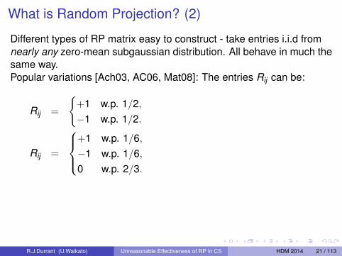
Different types of RP matrix easy to construct - take entries i.i.d fromnearly any zero-mean subgaussian distribution. All behave in much thesame way.
Popular variations [Ach03, AC06, Mat08]: The entries Rij can be:
Rij =
+1 w.p. 1/2,−1 w.p. 1/2.
Rij =
+1 w.p. 1/6,−1 w.p. 1/6,0 w.p. 2/3.
Rij =
N (0,1/q) w.p. q,0 w.p. 1− q.
Rij =
+1 w.p. q,−1 w.p. q,0 w.p. 1− 2q.
For the RH examples, taking q too small gives high distortion of sparsevectors [Mat08]. [AC06] get around this by using a randomizedorthogonal (normalized Hadamard) matrix to ensure w.h.p all datavectors are dense.
R.J.Durrant (U.Waikato) Unreasonable Effectiveness of RP in CS HDM 2014 21 / 113

What is Random Projection? (2)
Different types of RP matrix easy to construct - take entries i.i.d fromnearly any zero-mean subgaussian distribution. All behave in much thesame way.Popular variations [Ach03, AC06, Mat08]: The entries Rij can be:
Rij =
+1 w.p. 1/2,−1 w.p. 1/2.
Rij =
+1 w.p. 1/6,−1 w.p. 1/6,0 w.p. 2/3.
Rij =
N (0,1/q) w.p. q,0 w.p. 1− q.
Rij =
+1 w.p. q,−1 w.p. q,0 w.p. 1− 2q.
For the RH examples, taking q too small gives high distortion of sparsevectors [Mat08]. [AC06] get around this by using a randomizedorthogonal (normalized Hadamard) matrix to ensure w.h.p all datavectors are dense.
R.J.Durrant (U.Waikato) Unreasonable Effectiveness of RP in CS HDM 2014 21 / 113

Fast, sparse variants
Achlioptas ‘01 [Ach03]: Rij = 0 w.p. 2/3Ailon-Chazelle ‘06 [AC06]: Use x 7−→ PHDx , P random and sparse,Rij ∼ N (0,1/q) w.p 1/q, H normalized Hadamard (orthogonal) matrix,D = diag(±1) random. Mapping takes O
(d log d + qdε−2 log N
).
Ailon-Liberty ‘09 [AL09]: Similar construction to [AC06].O(d log k + k2).
Dasgupta-Kumar-Sarlos ‘10 [DKS10]: Use sequence of (dependent)random hash functions. O
(ε−1 log2(k/δ) log δ−1
)for
k ∈ O(ε−2 log δ−1).
Ailon-Liberty ‘11 [AL11]: Similar construction to [AC06]. O (d log d)
provided k ∈ O(ε−2 log N log4 d
).
R.J.Durrant (U.Waikato) Unreasonable Effectiveness of RP in CS HDM 2014 22 / 113

Generalizations of JLL to Manifolds
From JLL we obtain high-probability guarantees that, independently ofthe data dimension, random projection approximately preserves datageometry of a finite point set (for a suitably large k ). In particularnorms and dot products approximately preserved w.h.p.
JLL approach can be extended to (smooth, compact) Riemannianmanifolds: ‘Manifold JLL’
Key idea: Preserve ε-covering of smooth manifold under some metricinstead of geometry of data points. Replace N with correspondingcovering number M and take k ∈ O
(ε−2 log M
).
R.J.Durrant (U.Waikato) Unreasonable Effectiveness of RP in CS HDM 2014 23 / 113

Subspace JLLLet S be an s-dimensional linearsubspace. Let ε > 0. Fork = O
(ε−2s log(12/ε)
)[BW09] w.h.p. a
JLL matrix R satisfies ∀x , y ∈ S:(1− ε)‖x − y‖2d 6 ‖Rx − Ry‖2k 6(1 + ε)‖x − y‖2d
1 R linear, so no loss to take‖x − y‖ = 1.
2 Cover unit sphere in subspace withε/4-balls. Covering numberM = (12/ε)s.
3 Apply JLL to centres of the balls.k = O (log M) for this.
4 Extend to entire s-dimensionalsubspace by approximating any unitvector with one of the centres.
R.J.Durrant (U.Waikato) Unreasonable Effectiveness of RP in CS HDM 2014 24 / 113

Manifold JLL
Proof idea:1 Let M be a smooth s-dimensional
manifold in Rd (⇒ M is locally like alinear subspace).
2 Approximate manifold with tangentsubspaces.
3 Apply subspace-JLL on eachsubspace.
4 Union bound over subspaces topreserve large distances.
(Same basic approach can be used to preserve geodesic distances.)
R.J.Durrant (U.Waikato) Unreasonable Effectiveness of RP in CS HDM 2014 25 / 113

JLL for unions of axis-aligned subspaces (‘RIP’)
RIP = Restricted isometry property (more on this later).
Proof idea:
1 Note that s-sparse d-dimensionalvectors live on a union of
(ds
)s-dimensional subspaces.
2 Apply subspace-JLL to each s-flat.3 Apply union bound to all
(ds
)subspaces.
k = O(ε−2s log(12
εds ))
[BDDW08]
Comment: This is the canonical ‘compressed sensing’ settingassuming the sparse basis is known.
R.J.Durrant (U.Waikato) Unreasonable Effectiveness of RP in CS HDM 2014 26 / 113

Outline
1 Background and Preliminaries
2 Johnson-Lindenstrauss Lemma (JLL) and extensions
3 Applications of JLL (1)Approximate Nearest Neighbour SearchRP PerceptronMixtures of Gaussians
4 Compressed Sensing
5 Applications of JLL (2)
6 JLL- and CS-free Approaches
R.J.Durrant (U.Waikato) Unreasonable Effectiveness of RP in CS HDM 2014 27 / 113
Applications of Random Projection (1)
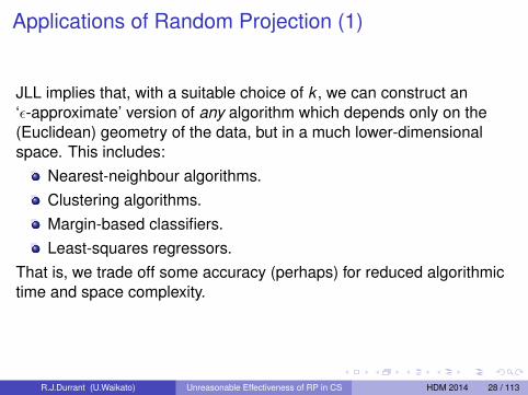
JLL implies that, with a suitable choice of k , we can construct an‘ε-approximate’ version of any algorithm which depends only on the(Euclidean) geometry of the data, but in a much lower-dimensionalspace. This includes:
Nearest-neighbour algorithms.Clustering algorithms.Margin-based classifiers.Least-squares regressors.
That is, we trade off some accuracy (perhaps) for reduced algorithmictime and space complexity.
R.J.Durrant (U.Waikato) Unreasonable Effectiveness of RP in CS HDM 2014 28 / 113

Using one RP...
Diverse motivations for RP in the literature:
To trade some accuracy in order to reduce computational expenseand/or storage overhead (e.g. kNN).To create a new theory of cognitive learning (RP Perceptron).To replace a heuristic optimizer with a provably correct algorithmwith performance guarantees (e.g. Mixture learning).To bypass the collection of lots of data then throwing away most ofit at preprocessing (Compressed sensing).
Solution in all cases: Work with random projections of the data.
R.J.Durrant (U.Waikato) Unreasonable Effectiveness of RP in CS HDM 2014 29 / 113

JLL-based approaches
Recall our two initial problem settings:Very high dimensional data (arity ∈ O (1000)) and very manyobservations (N ∈ O (1000)): Computational (time and spacecomplexity) issues.Very high dimensional data (arity ∈ O (1000)) and hardly anyobservations (N ∈ O (10)): Inference a hard problem. Bogusinteractions between features.
For this part of the talk we focus mainly on the first of these problems,i.e. reducing the complexity of large problems.
R.J.Durrant (U.Waikato) Unreasonable Effectiveness of RP in CS HDM 2014 30 / 113
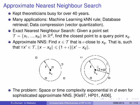
Approximate Nearest Neighbour SearchKept theoreticians busy for over 40 years.Many applications: Machine Learning kNN rule; Databaseretrieval; Data compression (vector quantization).Exact Nearest Neighbour Search: Given a point setT = x1, ..., xN in Rd , find the closest point to a query point xq.Approximate NNS: Find x ∈ T that is ε-close to xq. That is, suchthat ∀x ′ ∈ T , ‖x − xq‖ 6 (1 + ε)‖x ′ − xq‖.
The problem: Space or time complexity exponential in d even forsophisticated approximate NNS. [Kle97, HP01, AI06].
R.J.Durrant (U.Waikato) Unreasonable Effectiveness of RP in CS HDM 2014 31 / 113
Nearest Neighbour Search
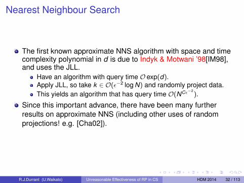
The first known approximate NNS algorithm with space and timecomplexity polynomial in d is due to Indyk & Motwani ’98[IM98],and uses the JLL.
Have an algorithm with query time O exp(d).Apply JLL, so take k ∈ O(ε−2 log N) and randomly project data.This yields an algorithm that has query time O(NCε−2
).
Since this important advance, there have been many furtherresults on approximate NNS (including other uses of randomprojections! e.g. [Cha02]).
R.J.Durrant (U.Waikato) Unreasonable Effectiveness of RP in CS HDM 2014 32 / 113

Neuronal RP Perceptron Learning
Motivation: How does the brainlearn concepts from a handful ofexamples when each examplecontains many features?Large margin⇒ ‘robustness’ ofconcept.Idea:
1 When the target concept robust,random projection of examples to alow-dimensional subspacepreserves the concept.
2 In the low-dimensional space, thenumber of examples and timerequired to learn concepts arecomparatively small.
R.J.Durrant (U.Waikato) Unreasonable Effectiveness of RP in CS HDM 2014 33 / 113

Definition. For any real number ` > 0, a concept in conjunction with adistribution D on Rd × −1,1, is said to be robust, ifPrx |∃x ′ : label(x) 6= label(x ′), and ‖x − x ′‖ 6 ` = 0.Given T = (x1, y1), ..., (xN , yN) ∼ DN labelled training set, R ∈Mk×da random matrix with zero-mean sub-Gaussian entries.Suppose T is a sample from a robust concept, i.e. ∃h ∈ Rd , ‖h‖ = 1s.t. ∀n ∈ 1, ...,N, yn · hT xn > `.
Algorithm1 Project T to T ′ = (Rx1, y1), ..., (RxN , yN) ⊆ Rk .2 Learn a perceptron hR in Rk from T ′ (i.e. by minimizing training
error).3 Output R and hR.
For a query point xq predict sign(hTRRxq).
R.J.Durrant (U.Waikato) Unreasonable Effectiveness of RP in CS HDM 2014 34 / 113

PAC Guarantees for RP PerceptronUsing known results on generalization for halfspaces [KV94], and onthe running time of Perceptron [MP69] in Rk , we use JLL to ensuretheir preconditions hold w.h.p.The results employed in [AV06] require classes to be separated by amargin ` in the dataspace and, for the randomly-projected perceptron,they then show that the classes remain `/2-separated w.h.p and thatall norms and dot products are also approximately preserved w.h.p.Taking L to be the squared diameter of the data and N the number oftraining examples, a PAC guarantee is obtained provided that:
k = O(
L`2· log(12N/δ)
)(1)
i.e. take k large enough to ensure all of the above conditions holdw.h.p.Comment: In [AV06] the authors obtain k = O
( 1`2· log( 1
ε`δ ))
by takingthe allowed misclassification rate as ε > 1
12N` . This somewhatobscures effect on upper bound on gen. error of # training points N.
R.J.Durrant (U.Waikato) Unreasonable Effectiveness of RP in CS HDM 2014 35 / 113

Provably Learning Mixtures of Gaussians
Mixtures of Gaussians (MoG) are among the most fundamentaland widely used statistical models. p(x) =
∑Ky=1 πyN (x |µy ,Σy ),
where N (x |µy ,Σy ) = 1(2π)d/2|Σy |1/2 exp(−1
2(x − µy )T Σ−1y (x − µy )).
Given a set of unlabelled data points drawn from a MoG, the goalis to estimate the mean µy and covariance Σy for each source.Greedy heuristics (such as Expectation-Maximization) widelyused for this purpose do not guarantee correct recovery of mixtureparameters (can get stuck in local optima of the likelihoodfunction).The first provably correct algorithm to learn a MoG from data isbased on random projections.
R.J.Durrant (U.Waikato) Unreasonable Effectiveness of RP in CS HDM 2014 36 / 113

AlgorithmInputs: Sample S: set of N data points in Rd ; m = number of mixturecomponents; ε,δ: resp. accuracy and confidence params. πmin:smallest mixture weight to be considered.(Values for other params derived from these via the theoreticalanalysis of the algorithm.)
1 Randomly project the data onto a k -dimensional subspace of theoriginal space Rd . Takes time O(Nkd).
2 In the projected space:For x ∈ S, let rx be the smallest radius such that there are > ppoints within distance rx of x .Start with S′ = S.For y = 1, ...,m:
Let estimate µ∗y be the point x with the lowest rx
Find the q closest points to this estimated center.Remove these points from S′.
For each y , let Sy denote the l points in S which are closest to µ∗y .3 Let the (high-dimensional) estimate µy be the mean of Sy in Rd .
R.J.Durrant (U.Waikato) Unreasonable Effectiveness of RP in CS HDM 2014 37 / 113

DefinitionTwo Gaussians N (µ1,Σ1) and N (µ2,Σ2) in Rd are said to bec-separated if ‖µ1 − µ2‖ > c
√d ·maxλmax(Σ1), λmax(Σ2). A mixture
of Gaussians is c-separated if its components are c-separated.
TheoremLet δ, ε ∈ (0,1). Suppose the data is drawn from a mixture of mGaussians in Rd which is c-separated, for c > 1/2, has (unknown)common covariance matrix Σ with condition numberκ = λmax(Σ)/λmin(Σ), and miny πy = Ω(1/m). Then,
w.p. > 1− δ, the centre estimates returned by the algorithm areaccurate within `2 distance ε
√dλmax;
if√κ 6 O(d1/2/ log(m/(εδ))), then the reduced dimension
required is k = O(log m/(εδ)), and the number of data pointsneeded is N = mO(log2(1/(εδ))). The algorithm runs in timeO(N2k + Nkd).
R.J.Durrant (U.Waikato) Unreasonable Effectiveness of RP in CS HDM 2014 38 / 113

The proof is lengthy but it starts from the following observations:A c-separated mixture becomes a (c ·
√1− ε)-separated mixture
w.p. 1− δ after RP. This is becauseJLL ensures that the distances between centers are preservedλmax(RΣRT ) 6 λmax(Σ)
RP makes covariances more spherical (i.e. condition numberdecreases).
It is worth mentioning that the latest theoretical advances [KMV12] onlearning of high dimensional mixture distributions under generalconditions (i.e. without the c-separability condition) in polynomial timealso use RP.At present this is a theoretical construction only - no concreteimplementation.
R.J.Durrant (U.Waikato) Unreasonable Effectiveness of RP in CS HDM 2014 39 / 113

10 years later...
R.J.Durrant (U.Waikato) Unreasonable Effectiveness of RP in CS HDM 2014 40 / 113

Outline
1 Background and Preliminaries
2 Johnson-Lindenstrauss Lemma (JLL) and extensions
3 Applications of JLL (1)
4 Compressed SensingSVM from RP sparse data
5 Applications of JLL (2)
6 JLL- and CS-free Approaches
R.J.Durrant (U.Waikato) Unreasonable Effectiveness of RP in CS HDM 2014 41 / 113

Compressed Sensing (1)
Often high-dimensional data is sparse in the following sense: There issome representation of the data in a linear basis such that most of thecoefficients of the data vectors are (nearly) zero in this basis. Forexample, image and audio data in e.g. DCT basis.Sparsity implies compressibility e.g. discarding small DCT coefficientsgives us lossy compression techniques such as jpeg and mp3.
Idea: Instead of collecting sparse data and then compressing it to(say) 10% of its former size, what if we just captured 10% of the data inthe first place?In particular, what if we just captured 10% of the data at random?Could we reconstruct the original data?
Compressed (or Compressive) Sensing [Don06, CT06].
R.J.Durrant (U.Waikato) Unreasonable Effectiveness of RP in CS HDM 2014 42 / 113

Compressed Sensing (2)
Problem: Want to reconstruct sparse d-dimensional signal x , with snon-zero coeffs. in sparse basis, given only k random measurements.i.e. we observe:
y = Rx , y ∈ Rk , R ∈Mk×d , x ∈ Rd , k d .
and we want to find x given y . Since R is rank k d no uniquesolution in general.However we also know that x is s-sparse...
R.J.Durrant (U.Waikato) Unreasonable Effectiveness of RP in CS HDM 2014 43 / 113

Compressed Sensing (3)
Basis Pursuit Theorem (Candes-Tao 2004)Let R be a k × d matrix and s an integer such that:
y = Rx admits an s-sparse solution x , i.e. such that ‖x‖0 6 s.R satisfies the restricted isometry property (RIP) of order (2s, δ2s)with δ2s 6 2/(3 +
√7/4) ' 0.4627
Then:x = arg min
x‖x‖1 : y = Rx
If R and x satisfy the conditions on the BPT, then we canreconstruct x perfectly from its compressed representation, usingefficient `1 minimization methods.We know x needs to be s-sparse. Which matrices R then satisfythe RIP?
R.J.Durrant (U.Waikato) Unreasonable Effectiveness of RP in CS HDM 2014 44 / 113

Restricted Isometry Property
Restricted Isometry PropertyLet R be a k × d matrix and s an integer. The matrix R satisfies theRIP of order (s, δ) provided that, for all s-sparse vectors x ∈ Rd :
(1− δ)‖x‖22 6 ‖Rx‖22 6 (1 + δ)‖x‖22
One can show that random projection matrices satisfying the JLL w.h.palso satisfy the RIP w.h.p provided that k ∈ O (s log d). [BDDW08]does this using JLL combined with a covering argument in theprojected space, finally union bound over all possible
(ds
)s-dimensional subspaces.N.B. For signal reconstruction, data must be sparse: no perfectreconstruction guarantee from random projection matrices if s > d/2.
R.J.Durrant (U.Waikato) Unreasonable Effectiveness of RP in CS HDM 2014 45 / 113

Compressed Learning
Intuition: If the data are s-sparse then one can perfectly reconstructthe data w.h.p from its randomly projected representation, providedthat k ∈ O (s log d).It follows that w.h.p no information was lost by carrying out the randomprojection.Therefore w.h.p one should be able to construct a classifier (orregressor) from the RP data which generalizes as well as the classifier(or regressor) learned from the original (non-RP) data.
R.J.Durrant (U.Waikato) Unreasonable Effectiveness of RP in CS HDM 2014 46 / 113

Fast learning of SVM from sparse data
Theorem (Calderbank et al. [CJS09])Let R be a k × d random matrix which satisfies the RIP. LetRS = (Rx1, y1), ..., (RxN , yN) ∼ DN .Let zRS be the soft-margin SVM trained on RS.Let w0 be the best linear classifier in the data domain with low hingeloss and large margin (hence small ‖w0‖).Then, w.p. 1− 2δ (over RS):
HD(zRS) 6 HD(w0) +O
(√‖w0‖2
(L2ε+
log(1/δ)
N
))(2)
where HD(w) = E(x ,y)∼D[1− ywT x ] is the true hinge loss of theclassifier in its argument, and L = maxn‖xn‖.
R.J.Durrant (U.Waikato) Unreasonable Effectiveness of RP in CS HDM 2014 47 / 113

The proof idea is somewhat analogousto that in Arriaga & Vempala, with severaldifferences:
Major:Data is assumed to be sparse.This allows using RIP instead ofJLL and eliminates thedependence of the required k onthe sample size N. Instead it willnow depend (linearly) on s.
Minor:Different classifierThe best classifier is not assumedto have zero error
R.J.Durrant (U.Waikato) Unreasonable Effectiveness of RP in CS HDM 2014 48 / 113

Proof sketch:Risk bound in [SSSS08] bounds the true SVM hinge loss of aclassifier learned from data from that of the best classifier. Usedtwice: once in the data space, and again in the projection space.By definition (of best classifier), the true error of the best classifierin projected space is smaller than that of the projection of the bestclassifier in the data space.From RIP, derive the preservation of dot-products (similarly aspreviously in the case of JLL) which is then used to connectbetween the two spaces.
R.J.Durrant (U.Waikato) Unreasonable Effectiveness of RP in CS HDM 2014 49 / 113

Outline
1 Background and Preliminaries
2 Johnson-Lindenstrauss Lemma (JLL) and extensions
3 Applications of JLL (1)
4 Compressed Sensing
5 Applications of JLL (2)RP LLS Regression
6 JLL- and CS-free Approaches
R.J.Durrant (U.Waikato) Unreasonable Effectiveness of RP in CS HDM 2014 50 / 113
Compressive Linear Least Squares Regression
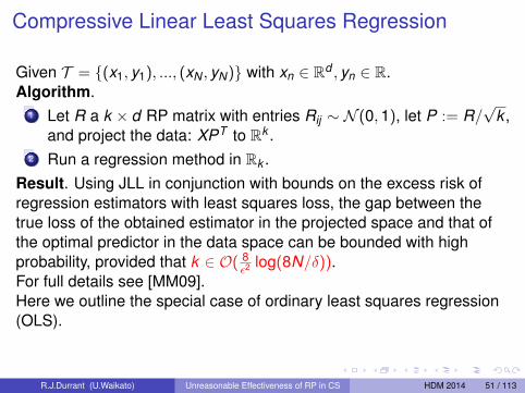
Given T = (x1, y1), ..., (xN , yN) with xn ∈ Rd , yn ∈ R.Algorithm.
1 Let R a k × d RP matrix with entries Rij ∼ N (0,1), let P := R/√
k ,and project the data: XPT to Rk .
2 Run a regression method in Rk .Result. Using JLL in conjunction with bounds on the excess risk ofregression estimators with least squares loss, the gap between thetrue loss of the obtained estimator in the projected space and that ofthe optimal predictor in the data space can be bounded with highprobability, provided that k ∈ O( 8
ε2log(8N/δ)).
For full details see [MM09].Here we outline the special case of ordinary least squares regression(OLS).
R.J.Durrant (U.Waikato) Unreasonable Effectiveness of RP in CS HDM 2014 51 / 113

Denote by X the design matrix with xi its rows, and Y a column vectorwith elements yi .Assume X is fixed (not random), and we want to learn an estimator βso that X β approximates E[Y |X ] .Definitions in Rd .Squared loss: L(w) = 1
N EY [‖Y − Xw‖2] (where EY denotes EY |X ).Optimal predictor: β = arg min
wL(w).
Excess risk of an estimator: R(β) = L(β)− L(β).For linear regression this is: (β − β)T Σ(β − β) where Σ = X T X/N.OLS estimator: β := arg min
w
1N ‖Y − Xw‖2
Proposition: OLS. If Var(Yi) 6 1 then EY [R(β)] 6 dN .
R.J.Durrant (U.Waikato) Unreasonable Effectiveness of RP in CS HDM 2014 52 / 113

Definitions in Rk .Square loss: LP(w) = 1
N EY [‖Y − (XPT )w‖2] (where EY denotes EY |X ).Optimal predictor: βP = arg min
wLP(w).
RP-OLS estimator: βP := arg minw
1N ‖Y − (XPT )w‖2
Proposition: Risk bound for RP-OLSAssume Var(Yi) 6 1, and let P as defined earlier. Then, fork = O(log(8N/δ)/ε2 and any ε, δ > 0, w.p. 1− δ we have:
EY [LP(βP)]− L(β) 6kN
+ ‖β‖2‖Σ‖traceε2 (3)
Comment: The argument in [MM09] uses JLL to obtain the excessrisk guarantee. Value of k obtained is suboptimal - log N term can beremoved (for an extended class of random matrices - includingnon-RIP/non-JLL matrices) using a more careful treatment - see[Kab14] for details.
R.J.Durrant (U.Waikato) Unreasonable Effectiveness of RP in CS HDM 2014 53 / 113

Outline
1 Background and Preliminaries
2 Johnson-Lindenstrauss Lemma (JLL) and extensions
3 Applications of JLL (1)
4 Compressed Sensing
5 Applications of JLL (2)
6 JLL- and CS-free ApproachesRP Fisher’s Linear Discriminant
Time Complexity AnalysisExperiments
RP Estimation of Distribution Algorithm
R.J.Durrant (U.Waikato) Unreasonable Effectiveness of RP in CS HDM 2014 54 / 113

Further approaches not leveraging JLL or CS
Recall our two initial problem settings:Very high dimensional data (arity ∈ O (1000)) and very manyobservations (N ∈ O (1000)): Computational (time and spacecomplexity) issues.Very high dimensional data (arity ∈ O (1000)) and hardly anyobservations (N ∈ O (10)): Inference a hard problem. Bogusinteractions between features.
For the remainder we will focus on the second problem, i.e. goodinference from next to no data.
R.J.Durrant (U.Waikato) Unreasonable Effectiveness of RP in CS HDM 2014 55 / 113

Some intuition and an idea
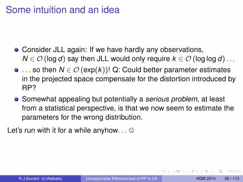
Consider JLL again: If we have hardly any observations,N ∈ O (log d) say then JLL would only require k ∈ O (log log d) . . .
. . . so then N ∈ O (exp(k))! Q: Could better parameter estimatesin the projected space compensate for the distortion introduced byRP?Somewhat appealing but potentially a serious problem, at leastfrom a statistical perspective, is that we now seem to estimate theparameters for the wrong distribution.
Let’s run with it for a while anyhow. . . ,
R.J.Durrant (U.Waikato) Unreasonable Effectiveness of RP in CS HDM 2014 56 / 113

Some intuition and an idea
Consider JLL again: If we have hardly any observations,N ∈ O (log d) say then JLL would only require k ∈ O (log log d) . . .
. . . so then N ∈ O (exp(k))! Q: Could better parameter estimatesin the projected space compensate for the distortion introduced byRP?Somewhat appealing but potentially a serious problem, at leastfrom a statistical perspective, is that we now seem to estimate theparameters for the wrong distribution.
Let’s run with it for a while anyhow. . . ,
R.J.Durrant (U.Waikato) Unreasonable Effectiveness of RP in CS HDM 2014 56 / 113

Guarantees without JLL
We can obtain guarantees for randomly-projected learning algorithmswithout directly applying the JLL, by using measure concentration andrandom matrix theoretic-based approaches. One application of suchan approach is the work on OLS by [Kab14]; here we will considerclassification and real-valued optimization.
Key Intuition: Projecting from a high-dimensional to a lowdimensional setting turns an ill-posed problem (i.e. with no uniquesolution) into a well-posed one (there is a unique solution).
Therefore we can view random projection as a way of regularizing theoriginal problem. But what kind of regularization? Can we say more?Most importantly, can we interpret the problem solved in the projectedspace in terms of the original problem?
R.J.Durrant (U.Waikato) Unreasonable Effectiveness of RP in CS HDM 2014 57 / 113

Applications (1)Classification with Fisher’s Linear
Discriminant
R.J.Durrant (U.Waikato) Unreasonable Effectiveness of RP in CS HDM 2014 58 / 113

Fisher’s Linear Discriminant (FLD)Supervised learningapproach.Simple and popularlinear classifier, inwidespread application.Classes are modelled asMVN distributions withsame covariance.Assign class label toquery point according toMahalanobis distancefrom class means.FLD decision rule:
h(xq) = 1
(µ1 − µ0)T Σ−1(
xq −(µ0 + µ1)
2
)> 0
R.J.Durrant (U.Waikato) Unreasonable Effectiveness of RP in CS HDM 2014 59 / 113

Randomly-projected Fisher’s Linear Discriminant
‘RP-FLD’: Learn the classifier and carry out the classification in the RPspace.Things we don’t need to worry about:
Important points lying in the null space of R: Happens withprobability 0.Problems mapping means, covariances in data space to RPspace: All well-defined due to linearity of R and E[·].
RP-FLD decision rule:
hR(xq) = 1
(µ1 − µ0)T RT(
RΣRT)−1
R(
xq −(µ0 + µ1)
2
)> 0
R.J.Durrant (U.Waikato) Unreasonable Effectiveness of RP in CS HDM 2014 60 / 113
The Problem
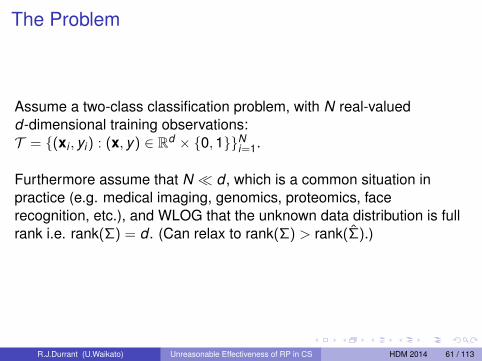
Assume a two-class classification problem, with N real-valuedd-dimensional training observations:T = (xi , yi) : (x, y) ∈ Rd × 0,1Ni=1.
Furthermore assume that N d , which is a common situation inpractice (e.g. medical imaging, genomics, proteomics, facerecognition, etc.), and WLOG that the unknown data distribution is fullrank i.e. rank(Σ) = d . (Can relax to rank(Σ) > rank(Σ).)
R.J.Durrant (U.Waikato) Unreasonable Effectiveness of RP in CS HDM 2014 61 / 113
Challenges (1)
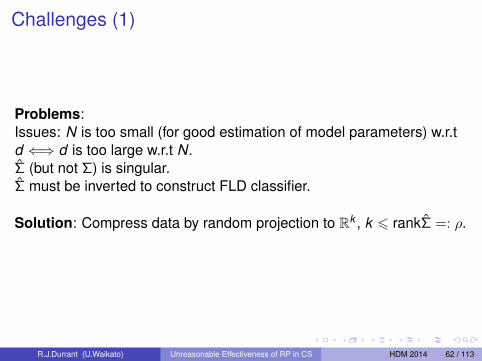
Problems:Issues: N is too small (for good estimation of model parameters) w.r.td ⇐⇒ d is too large w.r.t N.Σ (but not Σ) is singular.Σ must be inverted to construct FLD classifier.
Solution: Compress data by random projection to Rk , k 6 rankΣ =: ρ.
R.J.Durrant (U.Waikato) Unreasonable Effectiveness of RP in CS HDM 2014 62 / 113

Challenges (2)
It is known that, for a single randomly-projected (linear) classifier,expected misclassification error (w.r.t R) grows nearly exponentially ask 1 [DK13].
Solution:Recover performance using an ensemble of RP FLD classifiers [DK14].
Ensembles that use some form of randomization in the design of thebase classifiers have a long and successful history in machinelearning: E.g. bagging [Bre96]; random subspaces [Ho98]; randomforests [Bre01]; random projection ensembles [FB03, GBN05].
Comment: We also obtain substantial computational savings with ourapproach – details later.
R.J.Durrant (U.Waikato) Unreasonable Effectiveness of RP in CS HDM 2014 63 / 113
Our Questions
Can we recover (or improve on) the level of classificationperformance achieved in the data space, using our RP FLDensemble?Can we understand how the RP FLD ensemble acts to improveperformance?Can we overfit the data with too large an RP-FLD ensemble?Can we interpret the RP ensemble classifier parameters in termsof data space parameters?
R.J.Durrant (U.Waikato) Unreasonable Effectiveness of RP in CS HDM 2014 64 / 113
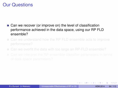

RP FLD Classifier Ensemble
For a single RP FLD classifier, the decision rule is given by:
1
(µ1 − µ0)T RT(
RΣRT)−1
R(
xq −µ1 + µ0
2
)> 0
which is the randomly projected analogue of the FLD decision rule. Forthe ensemble we use an equally weighted linear combination of RPFLD classifiers:
1
1M
M∑i=1
(µ1 − µ0)T RTi
(Ri ΣRT
i
)−1Ri
(xq −
µ1 + µ0
2
)> 0
(4)
Linear combination rules are a common choice for ensembles. Thisrule works well in practice and it is also tractable to analysis.
R.J.Durrant (U.Waikato) Unreasonable Effectiveness of RP in CS HDM 2014 65 / 113

Observation
We can rewrite decision rule as:
1
(µ1 − µ0)T 1
M
M∑i=1
RTi
(Ri ΣRT
i
)−1Ri
(xq −
µ1 + µ0
2
)> 0
Then, for average case analysis with a fixed training set, it is enough toconsider:
limM→∞
1M
M∑i=1
RTi
(Ri ΣRT
i
)−1Ri = E
[RT(
RΣRT)−1
R]
(Provided this limit exists).
R.J.Durrant (U.Waikato) Unreasonable Effectiveness of RP in CS HDM 2014 66 / 113

Theory(1):Regularization
For a fixed training set ρ, d are constant and 1 6 k 6 ρ is the integerregularization parameter (which we can choose).
Our analysis reveals that the (implicit) regularization schemeimplemented by the ensemble has a particularly pleasing form. Inparticular our ensemble implements:
Shrinkage regularization [LW04] in range of Σ.Ridge regularization [HTF01] in null space of Σ.
As k ρ− 1 we regularize less, and approach the performance ofpseudo-inverted FLD (i.e. we start to overfit).As k 1 we regularize more – very small choices of k typicallyunderfit.Sweet spot seems to be around k = ρ/2.
R.J.Durrant (U.Waikato) Unreasonable Effectiveness of RP in CS HDM 2014 67 / 113

Theory(2):Exact Error of Converged Ensemble
Theorem (Ensemble error with Gaussian classes)
Let xq ∼∑1
y=0 πyN (µy ,Σ), where Σ ∈Md×d is a full rank covariancematrix. Let R ∈Mk×d be a random projection matrix with i.i.d.
Gaussian entries and denote S−1R := ER
[RT(
RΣRT)−1
R]. Then the
exact error of the randomly projected ensemble classifier (4),conditioned on the training set, is given by:
1∑y=0
πy Φ
−12
(µ¬y − µy )T S−1R (µ0 + µ1 − 2µy )√
(µ1 − µ0)T S−1R ΣS−1
R (µ1 − µ0)
Comment: Generalization error is monotonic increasing inκ(S−1/2
R ΣS−1/2R ) - this condition number is bounded a.s. for a large
enough ensemble, but not for pseudo-inverted FLD – cf.[BL04].
R.J.Durrant (U.Waikato) Unreasonable Effectiveness of RP in CS HDM 2014 68 / 113

Theory (3): Finite sample guarantee for ensemble
Theorem (Generalization Error)
Let TN = (xi , yi)Ni=1 be a set of training data of size N = N0 + N1,subject to N < d and Ny > 1 ∀y. Let xq be a query point withGaussian class-conditionals xq|yq ∼ N (µy ,Σ), and letPryq = y = πy . Let ρ be the rank of the maximum likelihood estimateof the covariance matrix and let k < ρ− 1 be a positive integer. Thenfor any δ ∈ (0,1) and any training set of size N, the generalization errorof the converged ensemble is upper-bounded w.p. at least 1− δ by:
Prxq ,yq
(hens(xq) 6= yq) 61∑
y=0
πy Φ
(−
[g
(κ
(√2 log
5δ
))× . . .
. . .
[√‖Σ− 1
2 (µ1 − µ0)‖2 +dN
N0N1−√
2NN0N1
log5δ
]+
−
√dNy
(1 +
√2d
log5δ
)])
where κ(ε) is a high probability (w.r.t draws of TN ) upper bound on thecondition number of ΣS−1and g(·) is the function g(a) :=
√a
1+a .
R.J.Durrant (U.Waikato) Unreasonable Effectiveness of RP in CS HDM 2014 69 / 113

Comment
The principal terms in this bound are:1 The function g : [1,∞)→ (0, 1
2 ] which is a decreasing function ofits argument and here captures the effect of the mismatchbetween the estimated model covariance matrix S−1 and the trueclass-conditional covariance Σ, via a high-probability upper boundon the condition number of S−1Σ;
2 The Mahalanobis distance between the two class centres whichcaptures the fact that the better separated the classes are thesmaller the generalization error should be;
3 Antagonistic terms involving the sample size (N) and the numberof training examples in each class (N0,N1), capturing the effect ofclass imbalance - the more balanced the classes the tighter thebound.
R.J.Durrant (U.Waikato) Unreasonable Effectiveness of RP in CS HDM 2014 70 / 113

Time Complexity Analysis
R.J.Durrant (U.Waikato) Unreasonable Effectiveness of RP in CS HDM 2014 71 / 113

Time Complexity Analysis (1)Learning:In the data space, the cost of learning the FLD classifier is dominatedby inverting Σ, which is O
(d3) using Gauss-Jordan or O
(d2.807) using
Strassen’s algorithm.
For the RP ensemble the main cost comes from projecting the data (Mk × d matrix multiplications) plus M matrix inversions each O
(k3).
Taking M ∈ O(⌈
dk
⌉)so that the ensemble covariance is full rank w.p.
1, the time complexity on a single core is then:
O(
MkdN + Mk3)
= O(
d2N + dk2) O
(d3)
when N, k d
N.B. Parallel implementation of the ensemble straightforward, sparseRP matrices improve hidden constants considerably.Comment: Pseudo-inverse FLD is O
(Nd2) time complexity, diagonal
FLD O (d). Theory and experiments show classification performanceof these approaches can be very poor.
R.J.Durrant (U.Waikato) Unreasonable Effectiveness of RP in CS HDM 2014 72 / 113

Time Complexity Analysis (2)Classification:Can avoid randomly projecting a query point M times by averaging theindividual classifier decision rules. Bracket the argument to theensemble decision rule as:(
(µ1 − µ0)T 1M
M∑i=1
RTi
(Ri ΣRT
i
)−1Ri
)(xq −
µ1 + µ0
2
)to obtain a single linear classifier of the form h = w + b, w ∈ Rd ,b ∈ R, where:
w :=1M
M∑i=1
(µ1 − µ0)T RTi
(Ri ΣRT
i
)−1Ri =
1M
M∑i=1
wi
and
b := − 1M
M∑i=1
(µ1 − µ0)T RTi
(Ri ΣRT
i
)−1Ri
(µ1 + µ0
2
)=
1M
M∑i=1
bi
Complexity of classification then O (d) - same as data space FLD.R.J.Durrant (U.Waikato) Unreasonable Effectiveness of RP in CS HDM 2014 73 / 113

Experiments
R.J.Durrant (U.Waikato) Unreasonable Effectiveness of RP in CS HDM 2014 74 / 113

Experiments: Datasets
Table: Datasets
Name Source Sample size # featurescolon Alon et al. [ABN+99] 62 2000leukaemia Golub et al. [GST+99] 72 3571leukaemia lge Golub et al. [GST+99] 72 7129prostate Singh et al. [SFR+02] 102 6033duke West et al. [WBD+01] 44 7129dorothea NIPS 2003 [GGBHD03] 800 100000
First five datasets are real-valued, Dorothea is binary and very sparse.
R.J.Durrant (U.Waikato) Unreasonable Effectiveness of RP in CS HDM 2014 75 / 113

Experiments: ProtocolStandardized features to have mean 0 and variance 1. For genearrays ran experiments on 100 independent splits, for Dorotheaused single (competition) split.For gene arrays, in each split took 12 points for testing, rest fortraining. For Dorothea 800 points for training, 350 for testing.For data space experiments on colon and leukemia usedridge-regularized FLD and fitted regularization parameter using5-fold CV independently on each split, search in2−11,2−10, . . . ,2.For other gene array datasets we used diagonal FLD in the dataspace (size, no sig. diff. in error on colon, leuk.). For Dorotheaused Bernoulli NB without preprocessing the binary data.Compared performance with SVM with linear kernel andparameter C fitted by 5-fold CV, search in 2−10,2−9, . . . ,210,also compared with `1-regularized SVM.RP base learners: FLDs with full covariance and no regularization.
R.J.Durrant (U.Waikato) Unreasonable Effectiveness of RP in CS HDM 2014 76 / 113
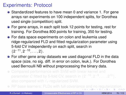
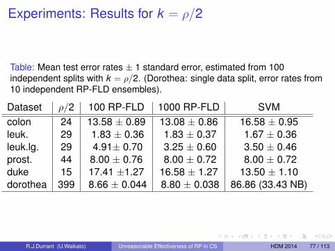
Experiments: Results for k = ρ/2
Table: Mean test error rates ± 1 standard error, estimated from 100independent splits with k = ρ/2. (Dorothea: single data split, error rates from10 independent RP-FLD ensembles).
Dataset ρ/2 100 RP-FLD 1000 RP-FLD SVMcolon 24 13.58 ± 0.89 13.08 ± 0.86 16.58 ± 0.95leuk. 29 1.83 ± 0.36 1.83 ± 0.37 1.67 ± 0.36leuk.lg. 29 4.91± 0.70 3.25 ± 0.60 3.50 ± 0.46prost. 44 8.00 ± 0.76 8.00 ± 0.72 8.00 ± 0.72duke 15 17.41 ±1.27 16.58 ± 1.27 13.50 ± 1.10dorothea 399 8.66 ± 0.044 8.80 ± 0.038 86.86 (33.43 NB)
R.J.Durrant (U.Waikato) Unreasonable Effectiveness of RP in CS HDM 2014 77 / 113

Experiments: Colon Cancer, Rij ∼ N (0,1)
0 10 20 30 4050
55
60
65
70
75
80
85
90
95
100
Projection dimension
Acc
urac
y(%
)
colon
FLD data spaceRP−FLDAveraging 10 RP−FLDsAveraging 100 RP−FLDsAveraging 3000 RP−FLDs
Figure: Plot shows test error rate versus k and error bars mark 1 standarderror estimated from 100 runs.
R.J.Durrant (U.Waikato) Unreasonable Effectiveness of RP in CS HDM 2014 78 / 113

Effect of k : Leukemia Large, Rij ∼ N (0,1)
0 10 20 30 40 5050
55
60
65
70
75
80
85
90
95
100
Projection dimension
Acc
urac
y(%
)
leukaemia large
FLD data spaceRP−FLDAveraging 10 RP−FLDsAveraging 100 RP−FLDsAveraging 3000 RP−FLDs
Figure: Plot shows test error rate versus k and error bars mark 1 standarderror estimated from 100 runs.
R.J.Durrant (U.Waikato) Unreasonable Effectiveness of RP in CS HDM 2014 79 / 113
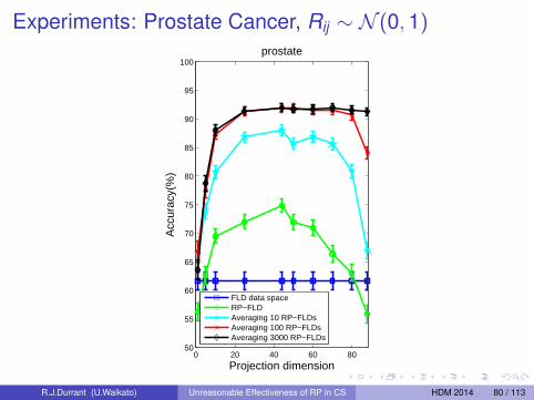
Experiments: Prostate Cancer, Rij ∼ N (0,1)
0 20 40 60 8050
55
60
65
70
75
80
85
90
95
100
Projection dimension
Acc
urac
y(%
)
prostate
FLD data spaceRP−FLDAveraging 10 RP−FLDsAveraging 100 RP−FLDsAveraging 3000 RP−FLDs
Figure: Plot shows test error rate versus k and error bars mark 1 standarderror estimated from 100 runs.
R.J.Durrant (U.Waikato) Unreasonable Effectiveness of RP in CS HDM 2014 80 / 113

Experiments: Duke Breast Cancer, Rij ∼ N (0,1)
0 5 10 15 20 25 3050
55
60
65
70
75
80
85
90
95
100
Projection dimension
Acc
urac
y(%
)
duke
FLD data spaceRP−FLDAveraging 10 RP−FLDsAveraging 100 RP−FLDsAveraging 3000 RP−FLDs
Figure: Plot shows test error rate versus k and error bars mark 1 standarderror estimated from 100 runs.
R.J.Durrant (U.Waikato) Unreasonable Effectiveness of RP in CS HDM 2014 81 / 113

Effect of k : Dorothea, Rij ∼ N (0,1)
0 100 200 300 40050
55
60
65
70
75
80
85
90
95
100
Projection dimension
Acc
urac
y (%
)
dorothea
Naive Bayes data spaceRP−FLDAveraging 10 RP−FLDsAveraging 100 RP−FLDsAveraging 1000 RP−FLDs
Figure: Plot shows test error rate versus k and error bars mark 1 standarderror estimated from 100 runs.
R.J.Durrant (U.Waikato) Unreasonable Effectiveness of RP in CS HDM 2014 82 / 113

Effect of M: Leukemia, Rij ∼ N (0,1)
0 20 40 60 80 10060
65
70
75
80
85
90
95
100
Nr classifiers
Acc
urac
y(%
)
leukemia
FLDRP−FLD k=5 AveragingRP−FLD k=25 AveragingRP−FLD k=100 AveragingRP−FLD k=500 Averaging
Figure: Plot shows test error rate versus ensemble size for various choices ofk . Error bars mark 1 s.e. estimated from 100 runs.
R.J.Durrant (U.Waikato) Unreasonable Effectiveness of RP in CS HDM 2014 83 / 113

Bernoulli RP Matrix: Leukemia, Rij ∼ −1,+1
0 20 40 60 80 10060
65
70
75
80
85
90
95
100
Nr classifiers
Acc
urac
y(%
)
leukemia
FLDRP−FLD k=5 AveragingRP−FLD k=25 AveragingRP−FLD k=100 AveragingRP−FLD k=500 Averaging
Figure: Plot shows test error rate versus ensemble size for various choices ofk . Error bars mark 1 s.e. estimated from 100 runs.
R.J.Durrant (U.Waikato) Unreasonable Effectiveness of RP in CS HDM 2014 84 / 113

Sparse RP Matrix: Leukemia, Rij ∼ −1,0,+1
0 20 40 60 80 10060
65
70
75
80
85
90
95
100
Nr classifiers
Acc
urac
y(%
)
leukemia
FLDRP−FLD k=5 AveragingRP−FLD k=25 AveragingRP−FLD k=100 AveragingRP−FLD k=500 Averaging
Figure: Plot shows test error rate versus ensemble size for various choices ofk . Error bars mark 1 s.e. estimated from 100 runs.
R.J.Durrant (U.Waikato) Unreasonable Effectiveness of RP in CS HDM 2014 85 / 113

Comparison with Majority Vote: Leukemia,Rij ∼ N (0,1)
0 20 40 60 80 10060
65
70
75
80
85
90
95
100
Nr classifiers
Acc
urac
y(%
)leukemia
FLDRP−FLD k=5 MajVoteRP−FLD k=25 MajVoteRP−FLD k=100 MajVoteRP−FLD k=500 MajVote
Figure: Plot shows test error rate versus ensemble size for various choices ofk for majority vote classifier. Error bars mark 1 s.e. estimated from 100 runs.
R.J.Durrant (U.Waikato) Unreasonable Effectiveness of RP in CS HDM 2014 86 / 113

Answers from Ensembles of RP-FLD
Can we recover (or improve on) level of classification performancein data space, using the RP FLD ensemble? YESCan we understand how the RP FLD ensemble acts to improveperformance? YESCan we overfit the data with the RP FLD ensemble? NO (withappropriate choice of k )Can we interpret the ensemble classifier parameters in terms ofdata space parameters? YES
R.J.Durrant (U.Waikato) Unreasonable Effectiveness of RP in CS HDM 2014 87 / 113

Applications (2)Large-scale Unconstrained Continuous
Optimization using EDA
R.J.Durrant (U.Waikato) Unreasonable Effectiveness of RP in CS HDM 2014 88 / 113

Estimation of Distribution Algorithm
EDA is a state-of-the art heuristic optimization scheme forunconstrained real optimization problems (in low-dimensional settings).Evolutionary algorithm-like approach - the main loop runs untilstopping criteria are met, and looks like:
1 Evaluate the objective function on a population of N candidatesolutions, and select the N ′ best individuals.
2 Assume these N ′ best individuals were drawn i.i.d from amultivariate Gaussian, and estimate its mean µ and covariancematrix Σ by µ and Σ using them.
3 Sample N new candidate solutions from the estimated distribution.4 Go to 1.
Comment: One can show that the eigenvalues of Σ act like ‘learningrates’ or ‘temperatures’, and good estimates of them imply (underconditions) an optimal search policy.
R.J.Durrant (U.Waikato) Unreasonable Effectiveness of RP in CS HDM 2014 89 / 113

Problems when Scaling Up EDA
In practice, objective functions evaluations are typically costly and soone tries to keep the population size N > N ′ as small as possible.Then:
If there are d parameters to optimize, and d is large, it is infeasibleto have a full-rank estimate of Σ (i.e. to have N ′ > d + 1).ML estimates of eigenvalues from few samples are very poor - theextrema are typically out by orders of magnitude.Sampling from a Gaussian in Rd is an O
(d3) operation, and this
is also infeasible if d is large.Diagonal constraints on Σ and other simple regularizers can workpoorly, and don’t solve the issue of the sampling cost.
We want an approach that will: Keep N small, improve the eigenvalueestimates, NEVER sample in Rd , avoid unjustified constraints on Σ,and still obtain good outcomes from the optimization scheme.
R.J.Durrant (U.Waikato) Unreasonable Effectiveness of RP in CS HDM 2014 90 / 113
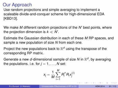
Our ApproachUse random projections and simple averaging to implement ascaleable divide-and-conquer scheme for high-dimensional EDA[KBD13].
We make M different random projections of the N ′ best points, wherethe projection dimension is k N ′.
Estimate the Gaussian distribution in each of these M RP spaces, andsample a new population of size N from each one.
Project the new populations back to Rd using the transpose of thecorresponding RP matrix.
Generate a new d-dimensional sample of size N in Rd , by averagingthe populations. i.e. for j = 1, . . . ,N set:
xj =1M
M∑i=1
RTi Rix
(i)j
R.J.Durrant (U.Waikato) Unreasonable Effectiveness of RP in CS HDM 2014 91 / 113

Why might this help?
−0.4 −0.2 0 0.2 0.4
−0.2
0
0.2
search points
−0.2 0 0.2
−0.2
0
0.2
0.4Ens−RP of search points, M=2
−0.5 0 0.5−0.4
−0.2
0
0.2
0.4
sample from Ens−RP (M=2)
−0.4−0.2 0 0.2 0.4−0.4
−0.2
0
0.2
0.4Ens−RP of search points, M=50
−0.2 0 0.2
−0.2
0
0.2
sample from Ens−RP (M=50)
−0.5 0 0.5
−0.2
0
0.2
sample from full ML estimate
−0.4 −0.2 0 0.2
−0.2
0
0.2
sample from diagonal estimate
Search using ML estimate isconstrained to lie in the rangeof Σ.
Diagonally-constrained EDAsearches whole space, butignores orientation of fitnessdensity of the parentpopulation.
Sampling from RP subspacesand averaging respectsorientation of the fitnessdensity, while still searchingwhole space.
R.J.Durrant (U.Waikato) Unreasonable Effectiveness of RP in CS HDM 2014 92 / 113

Does it work?
F2 F3 F5 F6 F8 F10 F11 F13 F15 F16 F18 F20
10−10
10−5
100
105
1000−dimensional multi−modal benchmark functions from the CEC’10 competition
RPens k=3 M=4d/k 6x10⁵ f.ev
CEC 2010 winner 6x10⁵ f.ev
DECC−CG, 3x10⁶ f.ev
MLCC, 3x10⁶ f.ev
separable single−group m−nonseparable, m=50
fully nonseparable
d/(2m)−group m−nonseparable, m=50
d/m−group m−nonseparable, m=50
(Small is good here.)
R.J.Durrant (U.Waikato) Unreasonable Effectiveness of RP in CS HDM 2014 93 / 113

Take me home!Random projections have a wide range of theoreticallywell-motivated and effective applications in machine learning anddata mining.In particular, random projections:
are easy to implement,can reduce time and space complexity of algorithms for smallperformance cost, andcan be used to construct parallel implementations of existingalgorithms.
Because random projection is independent of data distribution,theoretical analysis possible unlike many deterministicapproaches.In particular, can avoid worst-case guarantees for randomprojections but not (usually) for approaches such as PCA.In high dimensions RP matrices act like approximate isometries,preserving geometric properties of data well but in a lowerdimensional space.
R.J.Durrant (U.Waikato) Unreasonable Effectiveness of RP in CS HDM 2014 94 / 113

Thank You!
R.J.Durrant (U.Waikato) Unreasonable Effectiveness of RP in CS HDM 2014 95 / 113

References I[ABN+99] U. Alon, N. Barkai, D.A. Notterman, K. Gish, S. Ybarra, D. Mack, and A.J. Levine,
Broad patterns of gene expression revealed by clustering analysis of tumor andnormal colon tissues probed by oligonucleotide arrays, Proceedings of the NationalAcademy of Sciences 96 (1999), no. 12, 6745.
[AC06] N. Ailon and B. Chazelle, Approximate nearest neighbors and the fastjohnson-lindenstrauss transform, Proceedings of the thirty-eighth annual ACMsymposium on Theory of computing, ACM, 2006, pp. 557–563.
[Ach03] D. Achlioptas, Database-friendly random projections: Johnson-Lindenstrauss withbinary coins, Journal of Computer and System Sciences 66 (2003), no. 4, 671–687.
[AI06] A. Andoni and P. Indyk, Near-optimal hashing algorithms for approximate nearestneighbor in high dimensions, Foundations of Computer Science, 2006. FOCS’06.47th Annual IEEE Symposium on, IEEE, 2006, pp. 459–468.
[AL09] N. Ailon and E. Liberty, Fast dimension reduction using rademacher series on dualbch codes, Discrete & Computational Geometry 42 (2009), no. 4, 615–630.
[AL11] , An almost optimal unrestricted fast johnson-lindenstrauss transform,Proceedings of the Twenty-Second Annual ACM-SIAM Symposium on DiscreteAlgorithms, SIAM, 2011, pp. 185–191.
[AMS96] N. Alon, Y. Matias, and M. Szegedy, The space complexity of approximating thefrequency moments, Proceedings of the twenty-eighth annual ACM symposium onTheory of computing, ACM, 1996, pp. 20–29.
R.J.Durrant (U.Waikato) Unreasonable Effectiveness of RP in CS HDM 2014 96 / 113

References II[AV06] R. Arriaga and S. Vempala, An algorithmic theory of learning, Machine Learning 63
(2006), no. 2, 161–182.
[AV09] R. Avogadri and G. Valentini, Fuzzy ensemble clustering based on randomprojections for dna microarray data analysis, Artificial Intelligence in Medicine 45(2009), no. 2, 173–183.
[BD09] C. Boutsidis and P. Drineas, Random projections for the nonnegative least-squaresproblem, Linear Algebra and its Applications 431 (2009), no. 5-7, 760–771.
[BDDW08] R.G. Baraniuk, M. Davenport, R.A. DeVore, and M.B. Wakin, A Simple Proof of theRestricted Isometry Property for Random Matrices , Constructive Approximation 28(2008), no. 3, 253–263.
[BL04] P. Bickel and E. Levina, Some theory for Fisher’s linear discriminant function, ‘naıveBayes’, and some alternatives when there are many more variables thanobservations, Bernoulli 10 (2004), no. 6, 989–1010.
[BM01] E. Bingham and H. Mannila, Random projection in dimensionality reduction:applications to image and text data., Seventh ACM SIGKDD InternationalConference on Knowledge Discovery and Data Mining (KDD 2001) (F. Provost andR. Srikant, ed.), 2001, pp. 245–250.
[Bre96] L. Breiman, Bagging predictors, Machine learning 24 (1996), no. 2, 123–140.
[Bre01] , Random forests, Machine learning 45 (2001), no. 1, 5–32.
R.J.Durrant (U.Waikato) Unreasonable Effectiveness of RP in CS HDM 2014 97 / 113

References III
[BW09] R.G. Baraniuk and M.B. Wakin, Random projections of smooth manifolds,Foundations of Computational Mathematics 9 (2009), no. 1, 51–77.
[Cha02] M.S. Charikar, Similarity estimation techniques from rounding algorithms,Proceedings of the thirty-fourth annual ACM symposium on Theory of computing,ACM, 2002, pp. 380–388.
[CJS09] R. Calderbank, S. Jafarpour, and R. Schapire, Compressed learning: Universalsparse dimensionality reduction and learning in the measurement domain, Tech.report, Rice University, 2009.
[CT06] E.J. Candes and T. Tao, Near-optimal signal recovery from random projections:Universal encoding strategies?, Information Theory, IEEE Transactions on 52(2006), no. 12, 5406–5425.
[Das99] S. Dasgupta, Learning Mixtures of Gaussians, Annual Symposium on Foundationsof Computer Science, vol. 40, 1999, pp. 634–644.
[DF08] S. Dasgupta and Y. Freund, Random projection trees and low dimensionalmanifolds, Proceedings of the 40th annual ACM symposium on Theory ofcomputing, ACM, 2008, pp. 537–546.
[DG02] S. Dasgupta and A. Gupta, An Elementary Proof of the Johnson-LindenstraussLemma, Random Struct. Alg. 22 (2002), 60–65.
R.J.Durrant (U.Waikato) Unreasonable Effectiveness of RP in CS HDM 2014 98 / 113

References IV[DK10] R.J. Durrant and A. Kaban, Compressed Fisher Linear Discriminant Analysis:
Classification of Randomly Projected Data, Proceedings16th ACM SIGKDDConference on Knowledge Discovery and Data Mining (KDD 2010), 2010.
[DK12] , Error bounds for Kernel Fisher Linear Discriminant in Gaussian Hilbertspace, Proceedings of the 15th International Conference on Artificial Intelligenceand Statistics (AIStats 2012), 2012.
[DK13] RJ Durrant and A Kaban, Sharp generalization error bounds for randomly-projectedclassifiers, International Conference on Machine Learning (ICML 2013), vol. 16,2013, p. 21.
[DK14] R.J. Durrant and A. Kaban, Random Projections as Regularizers: Learning aLinear Discriminant from Fewer Observations than Dimensions, Machine Learning(In Press) (2014).
[DKS10] A. Dasgupta, R. Kumar, and T. Sarlos, A sparse johnson-lindenstrauss transform,Proceedings of the 42nd ACM symposium on Theory of computing, ACM, 2010,pp. 341–350.
[Don06] D.L. Donoho, Compressed Sensing, IEEE Trans. Information Theory 52 (2006),no. 4, 1289–1306.
[FB03] X.Z. Fern and C.E. Brodley, Random projection for high dimensional dataclustering: A cluster ensemble approach, International Conference on MachineLearning, vol. 20, 2003, p. 186.
R.J.Durrant (U.Waikato) Unreasonable Effectiveness of RP in CS HDM 2014 99 / 113

References V[FM03] D. Fradkin and D. Madigan, Experiments with random projections for machine
learning, Proceedings of the ninth ACM SIGKDD international conference onKnowledge discovery and data mining, ACM, 2003, pp. 522–529.
[GBN05] N. Goel, G. Bebis, and A. Nefian, Face recognition experiments with randomprojection, Proceedings of SPIE, vol. 5779, 2005, p. 426.
[GGBHD03] Isabelle Guyon, S Gunn, A Ben-Hur, and G Dror, NIPS 2003 Workshop on FeatureExtraction: Dorothea dataset, 2003.
[GST+99] T.R. Golub, D.K. Slonim, P. Tamayo, C. Huard, M. Gaasenbeek, J.P. Mesirov,H. Coller, M.L. Loh, J.R. Downing, M.A. Caligiuri, C.D. Bloomfield, and E.S. Lander,Molecular classification of cancer: class discovery and class prediction by geneexpression monitoring, Science 286 (1999), no. 5439, 531.
[Ho98] T.K. Ho, The random subspace method for constructing decision forests, PatternAnalysis and Machine Intelligence, IEEE Transactions on 20 (1998), no. 8,832–844.
[HP01] S. Har-Peled, A replacement for voronoi diagrams of near linear size, Foundationsof Computer Science, 2001. Proceedings. 42nd IEEE Symposium on, IEEE, 2001,pp. 94–103.
[HTF01] T. Hastie, R. Tibshirani, and J. Friedman, The elements of statistical learning; datamining, inference, and prediction, Springer, 2001.
R.J.Durrant (U.Waikato) Unreasonable Effectiveness of RP in CS HDM 2014 100 / 113

References VI
[HWB07] C. Hegde, M.B. Wakin, and R.G. Baraniuk, Random projections for manifoldlearningproofs and analysis, Neural Information Processing Systems, 2007.
[IM98] P. Indyk and R. Motwani, Approximate nearest neighbors: towards removing thecurse of dimensionality, Proceedings of the thirtieth annual ACM symposium onTheory of computing, ACM New York, NY, USA, 1998, pp. 604–613.
[Kab14] Ata Kaban, New bounds on compressive linear least squares regression,Proceedings of the 17-th International Conference on Artificial Intelligence andStatistics (AISTATS 2014), Journal of Machine Learning Research-ProceedingsTrack, vol. 33, 2014, pp. 448–456.
[KBD13] Ata Kaban, Jakramate Bootkrajang, and Robert John Durrant, Towards large scalecontinuous eda: A random matrix theory perspective, Proceeding of the FifteenthAnnual Conference on Genetic and Evolutionary Computation (New York, NY,USA), GECCO ’13, ACM, 2013, pp. 383–390.
[Kle97] J.M. Kleinberg, Two algorithms for nearest-neighbor search in high dimensions,Proceedings of the twenty-ninth annual ACM symposium on Theory of computing,ACM, 1997, pp. 599–608.
[KMN11] D. Kane, R. Meka, and J. Nelson, Almost optimal explicit johnson-lindenstraussfamilies, Approximation, Randomization, and Combinatorial Optimization.Algorithms and Techniques (2011), 628–639.
R.J.Durrant (U.Waikato) Unreasonable Effectiveness of RP in CS HDM 2014 101 / 113

References VII[KMV12] A.T. Kalai, A. Moitra, and G. Valiant, Disentangling gaussians, Communications of
the ACM 55 (2012), no. 2, 113–120.
[KV94] M.J. Kearns and U.V. Vazirani, An introduction to computational learning theory,MIT Press, 1994.
[Led01] M. Ledoux, The concentration of measure phenomenon, vol. 89, AmericanMathematical Society, 2001.
[LN14] Kasper Green Larsen and Jelani Nelson, The Johnson-Lindenstrauss lemma isoptimal for linear dimensionality reduction, arXiv preprint arXiv:1411.2404 (2014).
[LW04] O. Ledoit and M. Wolf, A well-conditioned estimator for large-dimensionalcovariance matrices, Journal of multivariate analysis 88 (2004), no. 2, 365–411.
[Mat08] J. Matousek, On variants of the johnson–lindenstrauss lemma, Random Structures& Algorithms 33 (2008), no. 2, 142–156.
[MM09] O. Maillard and R. Munos, Compressed Least-Squares Regression, NIPS, 2009.
[MP69] M. Minsky and S. Papert, Perceptrons, MIT press, 1969.
[Rec11] B. Recht, A simpler approach to matrix completion, Journal of Machine LearningResearch 12 (2011), 3413–3430.
[RR08] A. Rahimi and B. Recht, Random features for large-scale kernel machines,Advances in neural information processing systems 20 (2008), 1177–1184.
R.J.Durrant (U.Waikato) Unreasonable Effectiveness of RP in CS HDM 2014 102 / 113

References VIII
[Sar06] T. Sarlos, Improved approximation algorithms for large matrices via randomprojections, Foundations of Computer Science, 2006. FOCS’06. 47th Annual IEEESymposium on, IEEE, 2006, pp. 143–152.
[SFR+02] D. Singh, P.G. Febbo, K. Ross, D.G. Jackson, J. Manola, C. Ladd, P. Tamayo, A.A.Renshaw, A.V. D’Amico, J.P. Richie, E.S. Lander, M. Loda, P.W. Kantoff, T.R. Golub,and W.S. Sellers, Gene expression correlates of clinical prostate cancer behavior,Cancer cell 1 (2002), no. 2, 203–209.
[SR09] A. Schclar and L. Rokach, Random projection ensemble classifiers, EnterpriseInformation Systems (Joaquim Filipe, Jos Cordeiro, Wil Aalst, John Mylopoulos,Michael Rosemann, Michael J. Shaw, and Clemens Szyperski, eds.), LectureNotes in Business Information Processing, vol. 24, Springer, 2009, pp. 309–316.
[SSSS08] K. Sridharan, N. Srebro, and S. Shalev-Shwartz, Fast rates for regularizedobjectives, Advances in Neural Information Processing Systems 21, 2008,pp. 1545–1552.
[WBD+01] M. West, C. Blanchette, H. Dressman, E. Huang, S. Ishida, R. Spang, H. Zuzan,J.A. Olson, J.R. Marks, and J.R. Nevins, Predicting the clinical status of humanbreast cancer by using gene expression profiles, Proceedings of the NationalAcademy of Sciences 98 (2001), no. 20, 11462.
R.J.Durrant (U.Waikato) Unreasonable Effectiveness of RP in CS HDM 2014 103 / 113

Appendix
Proposition JLL for dot products.Let xn,n = 1 . . .N and u be vectors in Rd s.t. ‖xn‖, ‖u‖ 6 1.Let R be a k × d RP matrix with i.i.d. entries Rij ∼ N (0,1/
√k) (or with
zero-mean sub-Gaussian entries).Then for any ε, δ > 0, if k ∈ O
( 8ε2
log(4N/δ))
w.p. at least 1− δ wehave:
|xTn u − (Rxn)T Ru| < ε (5)
simultaneously for all n = 1 . . .N.
R.J.Durrant (U.Waikato) Unreasonable Effectiveness of RP in CS HDM 2014 104 / 113

Proof of JLL (1)
We will prove the following ‘distributional’ version of the JLL, and thenshow that this implies the original theorem:
Theorem (Distributional JLL)
Let ε ∈ (0,1). Let k ∈ N such that k > Cε−2 log δ−1, for a large enoughabsolute constant C. Then there is a random linear mappingP : Rd → Rk , such that for any unit vector x ∈ Rd :
Pr
(1− ε) 6 ‖Px‖2 6 (1 + ε)> 1− δ
No loss to take ‖x‖ = 1, since P is linear.Note that the projected dimension k depends only on ε and δ.Lower bound k ∈ Ω(ε−2 log δ−1) sharp for randomizeddimensionality reduction [KMN11, LN14].
R.J.Durrant (U.Waikato) Unreasonable Effectiveness of RP in CS HDM 2014 105 / 113

Proof of JLL (2)
Consider the following simple mapping:
Px :=1√k
Rx
where R ∈Mk×d with entries Riji.i.d∼ N (0,1).
Let x ∈ Rd be an arbitrary unit vector.We are interested in quantifying:
‖Px‖2 =
∥∥∥∥ 1√k
Rx∥∥∥∥2
:=
∥∥∥∥ 1√k
(Y1,Y2, . . . ,Yk )
∥∥∥∥2
=1k
k∑i=1
Y 2i =: Z
where Yi =∑d
j=1 Rijxj .
R.J.Durrant (U.Waikato) Unreasonable Effectiveness of RP in CS HDM 2014 106 / 113

Proof of JLL (3)
Recall that if Wi ∼ N (µi , σ2i ) and the Wi are independent, then∑
i Wi ∼ N(∑
i µi ,∑
i σ2i
). Hence, in our setting, we have:
Yi =d∑
j=1
Rijxj ∼ N
d∑j=1
E[Rijxj ],d∑
j=1
Var(Rijxj)
≡ N0,
d∑j=1
x2j
and since ‖x‖2 =
∑dj=1 x2
j = 1 we therefore have:
Yi ∼ N (0,1) , ∀i ∈ 1,2, . . . , k
it follows that each of the Yi are standard normal RVs and thereforekZ =
∑ki=1 Y 2
i is χ2k distributed.
Now we complete the proof using a standard Chernoff-boundingapproach.
R.J.Durrant (U.Waikato) Unreasonable Effectiveness of RP in CS HDM 2014 107 / 113

Proof of JLL (4)
PrZ > 1 + ε = Prexp(tkZ ) > exp(tk(1 + ε)), ∀t > 0Markov ineq. 6 E [exp(tkZ )] /exp(tk(1 + ε)),
Yi indep. =k∏
i=1
E[exp(tY 2
i )]/exp(tk(1 + ε)),
mgf of χ2 =[exp(t)
√1− 2t
]−kexp(−ktε),∀t < 1/2
next slide 6 exp(
kt2/(1− 2t)− ktε),
6 e−ε2k/8, taking t = ε/4 < 1/2.
PrZ < 1− ε = Pr−Z > ε− 1 is tackled in a similar way and givessame bound. Taking RHS as δ/2 and applying union bound completesthe proof (for a single x).
R.J.Durrant (U.Waikato) Unreasonable Effectiveness of RP in CS HDM 2014 108 / 113

Estimating (et√
1− 2t)−1
(et√1− 2t
)−1= exp
(−t − 1
2log(1− 2t)
),
Maclaurin S. for log(1− x) = exp(−t − 1
2
(−2t − (2t)2
2− . . .
)),
= exp(
(2t)2
4+
(2t)3
6+ . . .
),
6 exp(
t2(
1 + 2t + (2t)2 . . .))
,
= exp(
t2/ (1− 2t))
since 0 < 2t < 1
R.J.Durrant (U.Waikato) Unreasonable Effectiveness of RP in CS HDM 2014 109 / 113

Randomized JLL implies Deterministic JLL
Solving δ = 2 exp(−ε2k/8) for k we obtaink = 8/ε2 log δ−1 + log 2. i.e. k ∈ O
(ε−2 log δ−1).
Let V = x1, x2, . . . , xN an arbitrary set of N points in Rd and setδ = 1/N2, then k ∈ O
(ε−2 log N
).
Applying union bound to the randomized JLL proof for all(N
2
)possible interpoint distances, for N points we see a random JLLembedding of V into k dimensions succeeds with probability atleast 1−
(N2
) 1N2 >
12 .
We succeed with positive probability for arbitrary V . Hence weconclude that, for any set of N points, there exists linearP : Rd → Rk such that:
(1− ε)‖xi − xj‖2 6 ‖Pxi − Pxj‖2 6 (1 + ε)‖xi − xj‖2
which is the (deterministic) JLL.
R.J.Durrant (U.Waikato) Unreasonable Effectiveness of RP in CS HDM 2014 110 / 113

Comment (2)
In the proof of the randomized JLL the only properties we used whichare specific to the Gaussian distribution were:
1 Closure under additivity.2 Bounding squared Gaussian RV using mgf of χ2.
In particular, bounding via the mgf of χ2 gave us exponentially fastconcentration about mean norm.
Can do similar for matrices with zero-mean sub-Gaussian entries also:Sub-Gaussians are those distributions whose tails decay no slowerthan a Gaussian, e.g. practically all bounded distributions have thisproperty.
We obtain similar guarantees (i.e. up to small multiplicative constants)for sub-Gaussian RP matrices too!This allows us to get around issue of dense matrix multiplication indimensionality-reduction step.
R.J.Durrant (U.Waikato) Unreasonable Effectiveness of RP in CS HDM 2014 111 / 113

Proof of JLL for dot productsOutline: Fix one n, use parallelogram law and JLL twice, then useunion bound.
4(Rxn)T (Ru) = ‖Rxn + Ru‖2 − ‖Rxn − Ru‖2 (6)> (1− ε)‖xn + u‖2 − (1 + ε)‖xn − u‖2 (7)= 4xT
n u − 2ε(‖xn‖2 + ‖u‖2) (8)> 4xT
n u − 4ε (9)
Hence, (Rxn)T (Ru) > xTn u − ε, and because we used two sides of JLL,
this holds except w.p. no more than 2 exp(−kε2/8).The other side is similar and gives (Rxn)T (Ru) 6 xT
n u + ε except w.p.2 exp(−kε2/8).Put together, |(Rxn)T (Ru)− xT
n u| 6 ε · ‖x‖2+‖u‖2
2 6 ε holds except w.p.4 exp(−kε2/8).This holds for a fixed xn. To ensure that it holds for all xn together, wetake union bound and obtain eq.(5) must hold except w.p.4N exp(−kε2/8). Finally, solving for δ we obtain that k > 8
ε2log(4N/δ).
R.J.Durrant (U.Waikato) Unreasonable Effectiveness of RP in CS HDM 2014 112 / 113

R.J.Durrant (U.Waikato) Unreasonable Effectiveness of RP in CS HDM 2014 113 / 113