the university of chicago uncovering the...
TRANSCRIPT

THE UNIVERSITY OF CHICAGO
UNCOVERING THE RULES GOVERNING
PROTEIN FOLDING REACTIONS
A DISSERTATION SUBMITTED TO
THE FACULTY OF THE DIVISION OF THE PHYSICAL SCIENCES
IN CANDIDACY FOR DEGREE OF
DOCTOR OF PHILOSOPHY
DEPARTMENT OF PHYSICS
BY
MICHAEL CARL BAXA
CHICAGO, ILLINOIS
DECEMBER 2009

© 2009 Michael Carl Baxa
All rights reserved

To the love of my life, my best friend, Sybil

iv
Table of Contents
List of Figures ................................................................................................................................. vii
List of Tables ................................................................................................................................... ix
List of Equations ............................................................................................................................... x
List of Abbreviations ....................................................................................................................... xi
Acknowledgements ........................................................................................................................ xii
1 Introduction ............................................................................................................................. 1
1.1 Primary States of Proteins ................................................................................................ 2
1.1.1 The Native State ........................................................................................................ 2
1.1.2 The Unfolded State ................................................................................................... 5
1.1.3 The Transition State .................................................................................................. 6
1.2 Characterizing the Transition State .................................................................................. 7
1.2.1 The φ-analysis method .............................................................................................. 7
1.2.2 The ψ-analysis Method ............................................................................................. 9
1.2.3 Folding as a Search for the Native Topology .......................................................... 10
1.2.4 General Rules of Folding ......................................................................................... 12
1.3 Interpreting Experimental Data ..................................................................................... 14
1.4 Going Beyond the TS – Properties of the Unfolded State ............................................. 15
2 Quantifying the Structural Requirements of the Folding Transition State of Protein A and Other Systems ............................................................................................................................... 18
2.1 Introduction.................................................................................................................... 19
2.2 Materials and Methods .................................................................................................. 23
2.3 Results ............................................................................................................................ 24
2.3.1 ψ-analysis ................................................................................................................ 24
2.3.2 Lack of TS Heterogeneity ........................................................................................ 33
2.3.3 Amide H/D Kinetic Isotope Effect ............................................................................ 38
2.3.4 Properties of the TS ................................................................................................. 42

v
2.3.5 Relaxing the TS model ............................................................................................. 43
2.4 Discussion ....................................................................................................................... 49
2.5 Implications .................................................................................................................... 51
2.5.1 TS and Pathway Diversity ........................................................................................ 56
2.5.2 Comparisons with Theoretical Studies .................................................................... 57
2.6 Conclusion ...................................................................................................................... 60
3 ψ-constrained Simulations of Protein Folding Transition States: Implications for Calculating
φ ............................................................................................................................................... 62
3.1 Introduction.................................................................................................................... 63
3.1.1 Interpreting fractional ψ ......................................................................................... 63
3.1.2 Models of TS Heterogeneity .................................................................................... 64
3.1.3 Model of TS distortion ............................................................................................. 65
3.2 LD Simulations of the TSE ............................................................................................... 66
3.3 Fractional ψ .................................................................................................................... 71
3.4 Predicting φ from the TSE ............................................................................................... 81
3.5 Conclusion ...................................................................................................................... 82
4 Computing the Entropic Cost in Folding the Backbone of a Protein ..................................... 84
4.1 Introduction.................................................................................................................... 86
4.2 Methods ......................................................................................................................... 90
4.3 Results and Discussion ................................................................................................... 96
4.3.1 Unfolded State Ensemble ........................................................................................ 96
4.3.2 The Change in Configuration Entropy in Folding .................................................... 97
4.3.3 Ala→Gly Mutations ............................................................................................... 107
4.4 Conclusions................................................................................................................... 111
5 Conclusions and Future Steps ............................................................................................. 112
5.1 Summary of Thesis Within the View of Protein Folding .............................................. 112
5.2 Future Studies .............................................................................................................. 114
5.3 Origins of the 70% Rule ................................................................................................ 117
Appendix ..................................................................................................................................... 119

vi
References .................................................................................................................................. 125

vii
List of Figures
Figure 1.1: Contact-Contact Maps Highlight the Differences in Protein Topologies. ..................... 4
Figure 1.2: Correlation Between RCO and Log kf is Shown. .......................................................... 13
Figure 2.1: TS Models of Three 2-State Proteins That Satisfy ln kf –RCO Correlation Are Shown. 20
Figure 2.2: Metal-Dependent Chevrons Plots for BdpA ................................................................ 28
Figure 2.3: Kinetics as a Function of Zn2+ at Fixed [GdmCl] ......................................................... 29
Figure 2.4: ψo- and φ-values and Hydrogen Exchange Data for BdpA ......................................... 31
Figure 2.5: Absence of the E16-K50 Salt Bridge Between H1-H3 Contacts According to ψ- and φ-analysis .......................................................................................................................................... 32
Figure 2.6: Testing for Competing TS Composed of either H1-H2 or H2-H3 Microdomains ......... 35
Figure 2.7: Amide H/D Isotope Effects .......................................................................................... 39
Figure 2.8: Modeling the TS of BdpA using Langevin Dynamics Simulations ............................... 44
Figure 2.9: Modeling the TS of BdpA with Different Fractions of Native H-bonds ....................... 46
Figure 2.10: φ-values and model structures for the TS of other small domains ........................... 54
Figure 3.1: ψ-analysis Applied to Ub and the Two TS models ...................................................... 67
Figure 3.2: Distributions of Cβ-Cβ Separations for N, TSmax, and TSmin States ............................... 72
Figure 3.3: Illustrative Trajectories of Cβ-Cβ Separations and Hydrogen Bond Formation ........... 76
Figure 3.4: Hydrogen Bond Formation and Computed φ .............................................................. 78
Figure 4.1: Generating the Unfolded State Ensemble................................................................... 88
Figure 4.2: Correcting for Pixel Size in Entropy Calculations......................................................... 94
Figure 4.3: Predicted RDC Distribution for the Unfolded State Ensemble .................................... 98
Figure 4.4: Loss of Backbone Entropy During Folding ................................................................... 99
Figure 4.5: Loss of Backbone Entropy for Secondary Structure Elements and Amino Acids ....... 101
Figure 4.6: Nearest Neighbor Corrections to the Backbone Entropy .......................................... 106
Figure 4.7: Ramachandran Populations of Alanine Residues in Ub ............................................ 109
Figure 4.8: Ramachandran Populations of Glycine Residues in Ub ............................................ 110

viii
Figure 5.1: Proposed TS Structures and Predicted ψ-values for Model Proteins ........................ 115
ix
List of Tables
Table 2.1: Equilibrium and Kinetic Parameters for Divalent Metal Ion Bindinga .......................... 26
Table 2.2: Relative Metal Binding Affinities in the U, N, and TSs ................................................. 37
Table 4.1: Average Loss of Backbone Entropy, T∆S, in Foldinga,b ............................................... 103
x
List of Equations
Eqn 1.1: Definition of φ ................................................................................................................... 7
Eqn 1.2: Nonlinear Dependence of ∆∆Gf‡ on ∆∆Geq ....................................................................... 9
Eqn 1.3: Definition of ψ₀ ................................................................................................................. 9
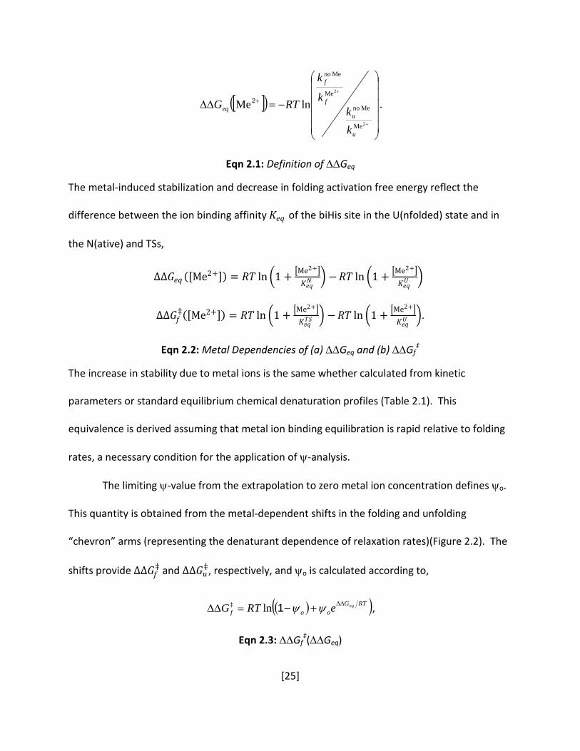
Eqn 2.1: Definition of ∆∆Geq ......................................................................................................... 25
Eqn 2.2: Metal Dependencies of (a) ∆∆Geq and (b) ∆∆Gf‡ ............................................................ 25
Eqn 2.3: ∆∆Gf‡(∆∆Geq) .................................................................................................................. 25
Eqn 3.1: Heterogeneous and Distorted Components of ψ ............................................................ 64
Eqn 4.1: Weeks-Chandler-Andersen Truncation of the Lennard-Jones Potential ......................... 91
Eqn 4.2: Residue-level Entropy from Ramachandran Probability Distributions ........................... 92
Eqn 4.3: Correlated Entropy Si,i+1 ................................................................................................... 92
Eqn 4.4: Backbone Entropy Corrected for Pixel Size ..................................................................... 93
Eqn A.1: ∆∆Gf‡(∆∆Geq) ................................................................................................................ 121
Eqn A.2: Definition of ψ .............................................................................................................. 121
Eqn A.3: Decomposing Folding Rate in Terms of TSpresent and TSabsent ........................................ 122
Eqn A.4: ψ Expressed in Terms of a Heterogeneous TSE ............................................................ 123
Eqn A.5: ψ Expressed in Terms of a Singular Distorted TS ......................................................... 123

xi
List of Abbreviations
Acp Acyl Phosphatase
BdpA B-domain of protein A
BiHis Bi-Histidine
CD Circular Dichroism
∆∆Geq Change in Equilibrium Stability
∆∆G𝑓𝑓‡ Change in Activation Free Energy.
G-S Amber 94 Garcia and Sanbonmatsu’s Modified Version of the Amber 94 Forcefield
GdmCl Guanidinium Chloride
HX Hydrogen Exchange
𝐾𝐾𝑒𝑒𝑒𝑒𝑈𝑈 Metal Ion Binding Affinity of the Denatured State
𝐾𝐾𝑒𝑒𝑒𝑒𝑁𝑁 Metal Ion Binding Affinity of the Native State
𝐾𝐾𝑒𝑒𝑒𝑒𝑇𝑇𝑇𝑇 Metal Ion Binding Affinity of the Transition State
kcal Kilocalorie (1 Kcal = 4.184 Kilojoules)
LD Langevin Dynamics
mol Mole
RCO Relative Contact Order
Rg Radius of Gyration
TSE Transition State Ensemble
Ub Ubiquitin
xii
Acknowledgments
I would like to thank my advisor, Tobin Sosnick, for his mentorship throughout my graduate
career at The University of Chicago. I am grateful for his guidance and the research
opportunities he has provided during my time in his lab. I am also thankful to Karl Freed for his
guidance and help in my computational research. Tom Witten and Frank Merritt, the other
members of my thesis committee, were excellent contributors with their constructive feedback
and their continual challenge to link protein folding back to the core principles of physics.
Biophysics allows me to apply my physics knowledge and background to relevant biological
problems, and this endeavor was truly a great interdisciplinary experience.
All past and present members of the Sosnick and Freed research groups provided advice
and assistance that helped guide my research projects. A few members of these labs went
above and beyond a standard lab member and the friendships we formed will last well beyond
my time at Chicago. There are additional members of the University community that provided
critical support in my research endeavors, and I am grateful for the time and assistance they
provided me.
I am grateful to the friends that I have made, especially to Eduard Antonyan for being my
study partner for the candidacy exam. I also greatly appreciate how my conversations with
Martin Tchernookov and Arjun Menon always reminded me of my love of physics.

xiii
Finally, words cannot express how much my wife, Sybil, has supported me throughout our
time together. I am deeply thankful for her love and support which has continually challenged
me to persevere and strive to be my best.

[1]
1 Introduction
Proteins are biological molecules that constitute a large majority of cellular machinery.
These molecules are linear heteropolymers of covalently linked amino acids, also referred to as
residues. There are twenty naturally occurring amino acids with varying physical properties in
biological systems. Protein folding is the process by which the protein adopts a unique three-
dimensional structure. Folding and unfolding reactions are involved in a wide variety of
biological regulatory mechanism (Hua et al. 1993; Dyson and Wright 2002; Dyson and Wright
2005; Sugase et al. 2007), and the role of folding errors have been implicated in many human
diseases including cancer (Bullock and Fersht 2001), amyloidoses (such as Alzheimer’s, Mad
Cow, and Huntington’s)(Kelly 1998; Prusiner 1998; Koo et al. 1999), and many others
(Thibodeau et al. 2005; Yue et al. 2005; Balch et al. 2008). Furthermore, understanding how a
sequence encodes for the unique native structure is a central problem in biophysics (Dill et al.
2007). The primary question that I will address in this thesis is whether one can develop
universal predictive principles that govern how proteins fold.
The current understanding of protein folding largely has been dominated by
experimental observation rather than theoretical predictions. Developing a theoretical model
that accurately describes real proteins is understandably difficult given the complexity of the
system. Beyond proposing general frameworks of folding that are not always easily falsifiable,
e.g. folding funnels (Dill and Chan 1997), much of the theoretical and computational work looks
for confirmation in existing experimental results. In the case of the B domain of protein A

[2]
(BdpA), for example, experimental data suggested that the third helix had the highest intrinsic
helical propensity (Bai et al. 1997). This observation was used as justification for simulations
that observe the third helix dominating the folding of the protein. Nevertheless, it was later
demonstrated experimentally that this helix plays a more subservient role (Baxa et al. 2008).
1.1 Primary States of Proteins
In order to identify rules of folding, I focus my investigation on small single domain
proteins, typically less than 200 residues in size. Surprisingly, many small proteins fold in
apparent two-state kinetic reactions in which no partially structured intermediates populate
(Jackson and Fersht 1991; Krantz et al. 2002a). The cooperative “all-or-none” manner with
which these proteins fold represents a useful simplification to describe the folding reaction. For
two-state proteins, the experimentalist is only able to directly observe the native and unfolded
states. However, methods exist to probe the structure of the polypeptide chain at the rate-
limiting step, highest free energy point, on the reaction surface. The chain conformations at
this point on the surface are termed the transition state ensemble (TSE). For the remainder of
this thesis, I will be referring to small two-state proteins when discussing the principles that
govern protein folding.
1.1.1 The Native State
High-resolution protein structures typically are determined by using either X-ray
crystallography or nuclear magnetic resonance (NMR) methods. At the time of this writing,
over 58,000 protein structures had been deposited in the Protein Data Bank
(http://www.rcsb.org/pdb) (Berman et al. 2000). In their native state, proteins tend to be

[3]
globular and well-packed with hydrophobic residues in the interior and charged residues on the
exterior. Intra-molecular backbone hydrogen bonds define the formation of regular secondary
structure elements. The two major secondary structure elements are the α-helix, defined by
hydrogen bonds formed between residues i and i+4 (Pauling et al. 1951), and the β-sheet,
where hydrogen bonds between aligned peptide segments produce a sheet-like structure
(Astbury 1933; Pauling and Corey 1951).
Proteins are commonly compared to each other according to the topology of their
structure, which can be described in terms of the secondary structure content, e.g. α, β, and
α/β. A protein’s topological complexity can be described by the number of short and long-
range contacts the backbone makes with itself in the folded state. This complexity can be put
into quantitative terms using the relative contact order (RCO) parameter (Plaxco et al. 1998).
The RCO is a measure of the average sequence separation between heavy atom contacts,
where a contact is defined according to some distance criteria, e.g. d ≤ 6 Å. Mapping all
contacts in a protein structure to an n × n matrix (n = number of residues) allows for a visual
comparison between different topologies. In such a representation, the RCO is the average
distance of contacts from the main diagonal (Figure 1.1). Other metrics of topology are used
(Goldenberg 1999; Ivankov et al. 2003; Bai et al. 2004; Pandit et al. 2006), but all of these
metrics are highly correlated. In Chapter 2, I discuss other advantages of using the RCO with
transition state ensembles (TSEs).

[4]
Figure 1.1: Contact-Contact Maps Highlight the Differences in Protein Topologies. Two heavy atoms on different residues form a contact if the distance between them is less than 6Å. Helical proteins, such as BdpA (upper left), form most of their contacts between amino acids separated by four residues, which results in a band of contacts aligned along the main diagonal. β-sheet contacts are characterized by off-diagonal contacts which are closer to the diagonal for hairpins (lower left) or much longer range contacts such as in Acp (lower right). The topology can be quantified by the relative contact order (RCO) parameter (upper right), where L is the length of the protein (number of amino acid residues), N is the number of contacts within 6 Å, and ∆seqk is the number of residues separating the kth interacting pair of non-hydrogen atoms. In a contact-contact map, the RCO is the average contact distance from the main diagonal, i.e. the average sequence separation between contacts.
0 10 20 30 40 50 600
10
20
30
40
50
600 10 20 30 40 50 60
0
10
20
30
40
50
60
10 20 30 40 50 60 70
10
20
30
40
50
60
70
10 20 30 40 50 60 70
10
20
30
40
50
60
70
10 20 30 40 50 60 70 80 90
102030405060708090
10 20 30 40 50 60 70 80 90
102030405060708090
BdpA: RCO = 0.10, kf ~ 104 s-1
Ub: RCO = 0.15, kf ~ 103 s-1 Acp: RCO = 0.20, kf ~ 1 s-1
∑=
∆=N
kkLN 1
1 seq·
RCO

[5]
1.1.2 The Unfolded State
The physical nature of the unfolded or denatured state ensemble of a protein is not
completely understood. Statistical coil models have been shown to reproduce the physical
characteristics of the unfolded state ensemble (Bernado et al. 2005; Jha et al. 2005a). As it
relates to our development of rules of folding, many of the properties of the unfolded state are
in direct contrast to those of the native state. The unfolded state is much more extended than
the globular native state. For the unfolded state, the radius of gyration, Rg ~ Nν, where ν =
0.598 ± 0.028, the critical exponent expected for a self-avoiding random walk (Kohn et al. 2004)
(compare to ν ~ 1/3 for a globular protein). Furthermore, unfolded states do not form stable
secondary structure elements, and spend most of the time sampling non-native backbone
geometries. Nevertheless, some people view this state as holding critical clues to the final fold.
There are multiple ways to make the unfolded state the thermodynamically favored
state. One way is to mutate one or more amino acids to other residues which are incompatible
with the native structure. Less permanent methods include adding increasing concentrations of
chemical denaturant (such as urea or guanidine hydrochloride) or raising the temperature (also
known as “cooking”). While the structural properties of the ensemble may vary, the
thermodynamics of folding remain independent of the mode of denaturation (Pfeil and Privalov
1976). It should be noted that for this thesis, I will be using chemical denaturation to generate
the unfolded ensembles.
[6]
1.1.3 The Transition State
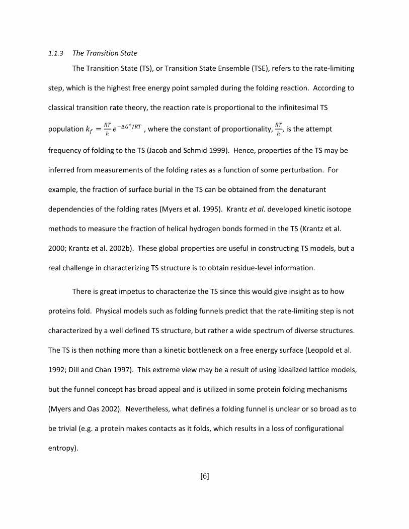
The Transition State (TS), or Transition State Ensemble (TSE), refers to the rate-limiting
step, which is the highest free energy point sampled during the folding reaction. According to
classical transition rate theory, the reaction rate is proportional to the infinitesimal TS
population 𝑘𝑘𝑓𝑓 = 𝑅𝑅𝑇𝑇ℎ𝑒𝑒−Δ𝐺𝐺‡/𝑅𝑅𝑇𝑇 , where the constant of proportionality,
𝑅𝑅𝑇𝑇ℎ
, is the attempt
frequency of folding to the TS (Jacob and Schmid 1999). Hence, properties of the TS may be
inferred from measurements of the folding rates as a function of some perturbation. For
example, the fraction of surface burial in the TS can be obtained from the denaturant
dependencies of the folding rates (Myers et al. 1995). Krantz et al. developed kinetic isotope
methods to measure the fraction of helical hydrogen bonds formed in the TS (Krantz et al.
2000; Krantz et al. 2002b). These global properties are useful in constructing TS models, but a
real challenge in characterizing TS structure is to obtain residue-level information.
There is great impetus to characterize the TS since this would give insight as to how
proteins fold. Physical models such as folding funnels predict that the rate-limiting step is not
characterized by a well defined TS structure, but rather a wide spectrum of diverse structures.
The TS is then nothing more than a kinetic bottleneck on a free energy surface (Leopold et al.
1992; Dill and Chan 1997). This extreme view may be a result of using idealized lattice models,
but the funnel concept has broad appeal and is utilized in some protein folding mechanisms
(Myers and Oas 2002). Nevertheless, what defines a folding funnel is unclear or so broad as to
be trivial (e.g. a protein makes contacts as it folds, which results in a loss of configurational
entropy).

[7]
Theoretical work tends to avoid viewing the folding reaction in multi-dimensional space
as having a distinct and well-defined TSE. However, this concept is practical and simplifies the
interpretation of many experiments. Further work discussed later will help to solidify an
understanding of the general principles of protein folding that can make specific predictions.
1.2 Characterizing the Transition State
1.2.1 The φ-analysis method
The traditional method used to characterize the transition state, termed φ-analysis, was
developed nearly 20 years ago and measures the energetic effect of removing side-chain
groups through mutation (Matthews 1987; Goldenberg et al. 1989; Fersht et al. 1992). The
folding kinetics and stability for a mutant (M) is measured and compared to the original (wild-
type – WT) folding behavior. In the tradition of Brønsted analysis, the change in folding energy,
ΔΔ𝐺𝐺𝑓𝑓𝑀𝑀,𝑊𝑊𝑇𝑇 = 𝑅𝑅𝑇𝑇 ln 𝑘𝑘𝑓𝑓𝑀𝑀 𝑘𝑘𝑓𝑓𝑊𝑊𝑇𝑇� , is taken to be linearly proportional to the change in stability,
ΔΔ𝐺𝐺𝑒𝑒𝑒𝑒𝑀𝑀,𝑊𝑊𝑇𝑇 , with the φ-value being the constant of proportionality, i.e.
WTMeq
WTf
Mf
WTMeq
WTMf
GkkRT
GG
,,
, ln∆∆
=∆∆
∆∆=φ .
Eqn 1.1: Definition of φ
The φ-value measures the energetic importance of the mutated side-group in the TS, relative to
its effect on the stability of the native state. When the TS is destabilized to the same extent as
the native state, the ensuing unity φ is interpreted as a native-like side-group interaction in the
TS. However, if the TS is not destabilized by the mutation while the native state is, the resulting
φ of zero is interpreted as the side-group having the same behavior in the TS as it does in the

[8]
unfolded state. Fractional φ can reflect either the presence of multiple TS structures or a partial
recovery of the native interactions in the TS, or any combination thereof. Mutational methods
can distinguish between these two cases (Fersht et al. 1992).
The application and interpretation of φ-analysis to proteins typically yield either a small
polarized TS (Riddle et al. 1999; Kim et al. 2000; McCallister et al. 2000; Nauli et al. 2001;
Northey et al. 2002a; Went and Jackson 2005) or a TS that is an expanded version of the native
state (Itzhaki et al. 1995). The apparent simplicity of this useful method masks many complex
issues, and the interpretation of φ is fraught with ambiguities. Measured φ tend to be
fractional, i.e. between 0.1 - 0.5 (Fersht et al. 1994; Khorasanizadeh et al. 1996; Kim et al. 1998;
Martinez et al. 1998; Moran et al. 1999; Bulaj and Goldenberg 2001; Krantz and Sosnick 2001;
Ozkan et al. 2001; Northey et al. 2002b; Krantz et al. 2004a), implying either multiple TS
structures or a single homogenous structure whose details are clouded by the meaning of
partial recovery of the native energy in the TS.
Fundamentally, the effects of the mutation are difficult to trace. Within the core of a
protein, the side-chain makes contacts with other residues. Thus, when removing this side-
chain, it is difficult to determine if some of these contacts were more affected than others.
Furthermore, TS relaxation has been observed such that the backbone will reorient to
accommodate the removal of a side-group and therefore underreport the mutated residue’s
presence in the TS (Bulaj and Goldenberg 2001). Non-native interactions in the TS will affect φ
(Feng et al. 2004) as will changes in secondary structure preferences. Multiple mutations at the
same position can address some of these ambiguities (Fersht et al. 1992; Northey et al. 2002b).
[9]
Translating all of these values into a structural picture of the TS is difficult, and often in place of
a picture, a characteristic verbal description is offered instead (Sato et al. 2004). However,
some suggest constructing structures from φ is possible (Paci et al. 2002).
1.2.2 The ψ-analysis Method
Sosnick and coworkers developed ψ-analysis as an alternative to the φ-analysis method,
which overcomes many of the ambiguities inherent in φ-analysis (Sosnick et al. 2006). A major
advantage is that the interaction between two specific partners is probed, so that the
information can be directly used to model a TS structure. Secondly, the effect is extrapolated
to the limit of no perturbation on the system. In this method, a metal binding bi-Histidine
(biHis) pair is mutated into a region of the protein, and the dependence of the folding kinetics
on divalent metal concentration is measured. The metal is in fast-equilibrium with the biHis
site and therefore binds whenever the site is in a competent (native-like) geometry (Bosco et al.
2009). Contrary to φ, the stabilization of the TS is a non-linear function of the native state
stabilization, i.e.
( )( )RTGoof
eqeRTG /‡ ln ∆∆+−=∆∆ ψψ1
Eqn 1.2: Nonlinear Dependence of ∆∆Gf‡ on ∆∆Geq
The single parameter ψo (sometimes referred to as just ψ), is defined by
0=∆∆∆∆∂
∆∆∂=
eqGeq
fo G
G‡
ψ
Eqn 1.3: Definition of ψ₀

[10]
and represents the extent of the probed site’s presence in the TS in the limit of zero
perturbation. Values of 0 and 1 imply either the absence or presence of the structural element
in the TS. Fractional ψ may be interpreted according to two different models, either TS
heterogeneity or TS distortion. For example, the heterogeneity model would state that a ψ of
0.5 implies that the site is natively formed in 50% of TSE, while the other 50% has the site
unformed. In the distortion model, the ψ-value reflects a metal binding affinity in the TS
intermediate between the unfolded and the folded states (see Appendix).
Prior to my thesis research, the ψ-analysis method has been used to characterize the
folding TSEs of two α/β proteins, ubiquitin (Ub) and acyl-phosphotase (Acp) (Krantz et al.
2004a; Pandit et al. 2006). In both cases, the TSE models exhibit extensive structure formation
and a high fraction of the native topology. Furthermore, the TSE of Ub constructed from the
zero and unity ψ is much more structured than that derived from extensive φ analysis (Sosnick
et al. 2004; Went and Jackson 2005). A comparison of the TSEψ and TSEφ suggests that the φ
data are reporting the rigidity of the TS structure, rather than the formation of structure
(Sosnick et al. 2004).
1.2.3 Folding as a Search for the Native Topology
The importance of forming the native topology during folding was implicated in studies
of the fast and slow folding events in cytochrome c (Sosnick et al. 1994; Sosnick et al. 1996).
The faster (two-sxtate) phase comes about when the heme group natively ligates with the
structure, while the slower phase is caused by a misfolding error which requires structural
rearrangements before folding can proceed to the native state. Hence, finding the native-like
[11]
topology was critical to fast (error-free) folding, and this native topology search is described as
a search-nucleation mechanism (Sosnick et al. 1996). The importance of topology was strongly
supported by Plaxco and coworker’s identification of a correlation between the folding rate of a
protein and its native topology, as measured by the RCO (Plaxco et al. 1998). This correlation is
reasonable if the limiting step is a global search process involving a polypeptide chain, rather
than a step related to a smaller scale event such as water expulsion from the hydrophobic core,
or the freezing in of the side-chain conformations – two major options being considered at the
time (Sosnick et al. 1994; Sosnick et al. 1996). For example, a three-helix bundle assumes many
more local contacts than long range contacts and thus would have less difficulty folding to its
native state than a protein like Acp, which must dock its C-terminus with the middle of the
sequence.
In addition to searching for the native topology, there is evidence that proteins fold by
concurrently forming secondary and tertiary structural units. Krantz et al. measured hydrogen
bond formation in the TS by exploiting the weak destabilizing effect of deuterium substitution
(Krantz et al. 2000). Similar to mutational φ-analysis, the effect of deuterium substitution on
the stabilities of the TS and native state are compared, and a φH-D value reports the fraction of
helical hydrogen bonds formed in the TS. For α-helical proteins, the fraction of helical
hydrogen bonds and the fraction of surface burial in the TS agree very well (Krantz et al. 2002b).
The presence of hydrogen bonds in the TS suggests that they are formed along the pre-
TS pathway as hydrophobic residues are buried. Rearranging the backbone to form hydrogen
bonds requires burying surface area. Inversely, burying surface area will potentially require

[12]
breaking hydrogen bonds and forming intra-mainchain hydrogen bonds. Native state hydrogen
exchange experiments on cytochrome c observed successive formation of structural units
(foldons) as folding progressed from the TS to the native state (Bai et al. 1995). There is no
reason to assume that the physics governing pre-TS folding differs significantly from post-TS
behavior, so folding to the TS is believed to be characterized by the successive formation of
foldons as well.
1.2.4 General Rules of Folding
The measured TSEs for Ub and Acp (Krantz et al. 2004a; Pandit et al. 2006) suggest that
the search-nucleation mechanism may be made more quantitative. For both proteins, the TS
models adopts the same fraction of the respective native topology, i.e. RCOTS ~ 0.7·RCON. This
observation points to a possible rule of folding underlying the correlation between the folding
rate and topology. A quantitative rule of folding would make strong statements regarding
allowable TS models as well as provide a framework in which to discuss folding mechanisms.
Ub and Acp are both α/β proteins that are located on the slower folding region of the ln kf -
RCO correlation (Figure 1.2) (Plaxco et al. 1998). In order to develop general rules of folding, it
is necessary to characterize the TS of a protein with a simpler topology that folds faster.
The B domain of protein A (BdpA) is a fast-folding three-helix bundle with low RCO. In
addition, it has the added benefit of having been extensively studied, yet no consensus exists
regarding the structure of the TS. This protein has been used as a model system for the
diffusion-collision mechanism of folding (Myers and Oas 2001). In this mechanism, folding is

[13]
Figure 1.2: Correlation Between RCO and Log kf is Shown.
The RCO values of the three proteins studied using ψ-analysis span the observed RCO range. The best linear fit to the data is represented by the red line. Data in this plot are taken from Refs. (Plaxco et al. 1998; Maxwell et al. 2005).
0.08 0.16 0.24
0
4
8
BdpA
log
k f
Relative Contact Order
ubiquitin
ctAcp
[14]
initiated first by the formation of the secondary structure elements prior to the formation of
inter-helical contacts, despite the relatively low intrinsic helical propensity (Bai et al. 1997).
Many computational simulations of BdpA invoke this mechanism when discussing their results
(Baxa et al. 2008), but this may also be a reflection of α-helical bias in the construction of
forcefields (Zaman et al. 2003). Other computational work on this protein have invoked other
mechanisms to describe the folding pathway (Wolynes 2004). Mutational φ-analysis yielded
many fractional values and was only able to implicate the role of the center helix in the TS.
Given this extensive ambiguity regarding its folding behavior, BdpA represents an ideal
protein with which to apply ψ-analysis and clarify the nature of the TS while also quantitatively
evaluating the extent of native-like topology in the TS. In Chapter 2, I discuss the experimental
and computational results for this protein and the proposal of the “70% Rule”, which posits that
proteins fold through TSEs that adopt ~70% of the native state topology (as measured by the
RCO).
1.3 Interpreting Experimental Data
Prior to the development of ψ-analysis, the primary data available for characterizing TS
structures was φ-analysis. As a result, many computational studies either compare folding
trajectories to experimental φ or predict φ from simulations and compare to experiment. This
assumes, though, that a valid equivalency can be made between the simulated calculations and
the experimental data. It is typically assumed in the literature that the experimental values,
which are measures of free energies, can be recapitulated in simulation by counting the
[15]
number of (native) contacts (Varnai et al. 2008; Yang et al. 2008), although a few other
comparisons have been made (Cheng et al. 2005).
The structural interpretation of ψ-values is much more straightforward, and, as such, I
am interested in being able to computationally model ψ. A unity ψ implies native-like binding
affinity in the TS, and therefore the simplest assumption is that the site adopts a native-like
configuration. Likewise, a zero ψ implies the site is not binding competent in the TS, and
therefore the site is unfolded-like in the TS. Using this set of assumptions, I construct TS
models of Ub and relax these structures using all-atom Langevin dynamics in Chapter 3. The
simulated TSE models provide structural insight into different interpretations of fractional ψ,
i.e. heterogeneity versus distortion. The TSEs were developed from the unambiguous zero and
unity ψ, and therefore, I am able to benchmark whether simulated and experimental φ will
necessarily agree. From these results, I discuss the implications for calculating φ from
simulations.
1.4 Going Beyond the TS – Properties of the Unfolded State
Ideally, I would like to understand how a protein folds based on sequence alone. This
would include a precise understanding of the nature of the unfolded state ensemble, which is
where folding begins, and which forms the thermodynamic reference state for stability. Recent
work by Jha et al. has shown that the unfolded state can be well described at the residue level
using a statistical coil model (Jha et al. 2005a). The conformations that a residue adopts are
biased by the chemical identity and conformation of nearest neighbors, thus reducing the

[16]
conformational diversity in the unfolded state (Pappu et al. 2000; Zaman et al. 2003; Jha et al.
2005b).
With a realistic unfolded state ensemble, I can more confidently calculate the change in
thermodynamic properties as a protein folds. The loss of backbone and side-chain
conformational entropy in the protein is the largest unfavorable quantity in the over-all stability
of the native state. However, entropy changes associated with the desolvation of hydrophobic
groups (release of water) offset the conformational entropy to a certain extent (Yu et al. 1994).
The change in conformational entropy has been measured to be about 1.5 kcal·mol-1 per
residue, which at 298 K is equivalent to an approximate ten-fold reduction in the number of
accessible states (Brandts 1964). Both side-chain and backbone conformations are included in
this measurement, and the two are inseparable because the states accessible to the side-chains
rotomers depend on what conformation the backbone has adopted. Others have made
calculations of the change in backbone entropy using other models (Nemethy and Scheraga
1965; Yang and Honig 1995; D'Aquino et al. 1996; Wang and Purisima 1996; Yang and Kay 1996;
Alexandrescu et al. 1998; Thompson et al. 2002; Scott et al. 2007). With a realistic unfolded
state ensemble model, I report calculations of the backbone conformational entropy associated
with folding Ub in Chapter 4. Computing the reduction in entropy of each residue due to
correlated motions required enriching the unfolded state ensemble with Langevin dynamics. I
discuss our results as they relate to our understanding of the unfolded state ensemble.
Finally in Chapter 5, I frame the results of Chapters 2-4 in the context of our
understanding of how proteins fold. I also discuss future projects that may help further

[17]
elucidate the principles that govern protein folding, especially the possible origins of the “70%
Rule”.
[18]
2 Quantifying the Structural Requirements of the Folding Transition State of Protein A and Other Systems
Much of the material in this chapter has been published (Baxa et al. 2008).
Abstract
The B-domain of protein A (BdpA) is a small 3-helix bundle that has been the subject of
considerable experimental and theoretical investigation. Nevertheless, a unified view of the
structure of the transition state ensemble (TSE) is still lacking. To characterize the TSE of this
surprisingly challenging protein, we apply a combination of ψ-analysis (which probes the role of
specific side-chain to side-chain contacts) and kinetic H/D amide isotope effects (which
measures hydrogen bond content), building upon previous studies using mutational φ-analysis
(which probes the energetic influence of side chain substitutions). The second helix (H2) is
folded in the TSE, while helix formation appears just at the carboxy and amino termini of the
first and third helices, respectively. The experimental data suggest a homogenous, yet plastic
TS with a native-like topology. This study generalizes our earlier conclusion, based on two
larger α/β proteins, that the TSEs of most small proteins achieve ~70% of their native state’s
relative contact order. This high percentage limits the degree of possible TS heterogeneity and
requires a re-evaluation of the structural content of the TSE of other proteins, especially when
they are characterized as small or polarized.

[19]
2.1 Introduction
The B-domain of protein A, BdpA, has been the focus of considerable experimental (Bai
et al. 1997; Myers and Oas 2001; Arora et al. 2004; Dimitriadis et al. 2004; Sato et al. 2004; Vu
et al. 2004a; Vu et al. 2004b; Sato et al. 2006; Sato and Fersht 2007) and theoretical
investigation (Sato et al. 2004; Wolynes 2004) due to its simple 3-helix bundle topology (Figure
2.1A), small size (60 residues), two-state folding behavior, and fast folding rate. However, a
consensus is still lacking concerning the structural content of its TSE (Sato et al. 2004; Wolynes
2004; Itoh and Sasai 2006). After extensive studies using φ-analysis, the participation of helices
H1 and H3 in the TSE remains unclear (Sato and Fersht 2007). Similarly, the predicted helical
content of the TS varies considerably among the theoretical treatments (Sato et al. 2004;
Wolynes 2004). Some studies emphasize the presence of H1-H2 or H2-H3 microdomains, while
others suggest the presence of all three helices (Alonso and Daggett 2000). To resolve these
uncertainties, further information is required.
We have developed ψ-analysis (Krantz and Sosnick 2001), in part to provide structural
models of TSEs. This counterpart to mutational φ-analysis (Matthews 1987; Fersht et al. 1992;
Goldenberg 1992) proceeds by introducing bi-Histidine (biHis) metal ion binding sites at specific
positions on the protein surface. Upon addition of metal ions, these sites stabilize secondary
and tertiary structures because an increase in the metal ion concentration stabilizes the
interaction between the two histidine partners (Appendix). The metal-induced stabilization of
the TSE relative to the native state is represented by the ψ-value and directly reports the
[20]
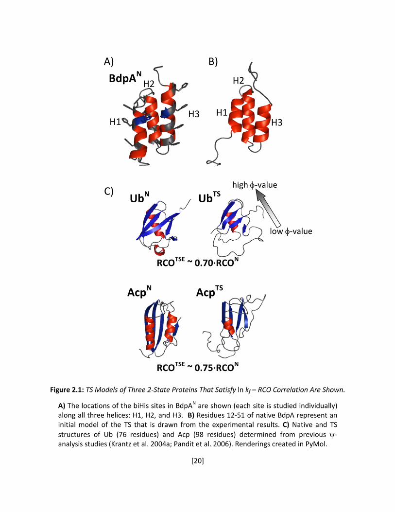
Figure 2.1: TS Models of Three 2-State Proteins That Satisfy ln kf – RCO Correlation Are Shown. A) The locations of the biHis sites in BdpAN are shown (each site is studied individually) along all three helices: H1, H2, and H3. B) Residues 12-51 of native BdpA represent an initial model of the TS that is drawn from the experimental results. C) Native and TS structures of Ub (76 residues) and Acp (98 residues) determined from previous ψ-analysis studies (Krantz et al. 2004a; Pandit et al. 2006). Renderings created in PyMol.
A)
B)
C)
BdpAN
UbN
AcpTS
UbTS
AcpN
RCOTSE ~ 0.70·RCON
RCOTSE ~ 0.75·RCON
high φ-value
low φ-value
H1
H2
H3
H1
H2
H3
[21]
proximity of the two partners in the TSE. The ψ-value depends on the degree to which the
biHis site is formed in the TSE. Values of zero or one indicate that the biHis site is absent or
fully native-like in the TSE, respectively. Fractional values indicate that the biHis site recovers
only part of the binding-induced stabilization of the native state. Examples of this partial
recovery include sites having non-native ion binding affinity or sites being formed in a
subpopulation of the TSE. The method is particularly well suited for identifying the side-chain
to side-chain contacts that define the TS’s topology and structure. The mutational counterpart,
φ-analysis, reports on the energetic influence of altering side chains and can underestimate the
structural content of the TS (Bulaj and Goldenberg 2001; Krantz and Sosnick 2001; Krantz et al.
2004a; Sosnick et al. 2004) due to chain relaxation and accommodation or to non-native
interactions (Feng et al. 2004; Neudecker et al. 2006).
A second motivation for this study emanates from previous ψ-analyses of ubiquitin (Ub)
and acyl phosphatase (Acp) (Figure 2.1C) where we conjecture that the TSE’s of two-state
proteins share a common and high fraction of their respective native topology (Pandit et al.
2006; Sosnick et al. 2006). This conjecture rests partly on the observation that the logarithm of
the folding rate for these proteins strongly correlates with the structural complexity of the
native state (Goldenberg 1999; Ivankov et al. 2003; Bai et al. 2004; Pandit et al. 2006), for
example, as defined by the RCO (Plaxco et al. 1998) (Figure 2.1D). In addition, ψ-analysis
indicates that the TSEs of Ub and Acp have RCOTS ~ 0.7-0.8 RCON (Krantz et al. 2004a; Pandit et
al. 2006; Sosnick et al. 2006). These observations combine to suggest that TSs of other proteins
obeying the known correlation of Figure 1.2 also acquire a similar fraction of their native state’s
[22]
RCO. However, Ub and Acp are both α/β proteins with intermediate to high RCOs (0.15 and
0.20, respectively). A test of the generality of this suggestion requires the determination of the
RCOTS of a helical protein with a low native RCO. BdpA is an excellent candidate, with an RCO of
0.10, lying at the lower end of the observed RCO range.
As reported in many previous studies of BdpA, we find that the TSE is challenging to
characterize. Many ψ-values are fractional, as are the φ-values (Sato et al. 2004). However, re-
measuring ψ in the background of additional mutations indicates that the fractional ψ-values
do not arise from competing TSEs composed of either H1-H2 or H2-H3 microdomains, a
possibility suggested by the symmetry of the protein and theoretical studies (Itoh and Sasai
2006). Furthermore, the kinetic amide H/D isotope effect (Kentsis and Sosnick 1998; Krantz et
al. 2000; Krantz et al. 2002a; Krantz et al. 2002b; Shi et al. 2002; Meisner and Sosnick 2004)
indicates that the TSE has ~70% of the native helical content. This critical information indicates
that the TS contains helix H2 along with half of both H1 and H3 docked against each other and
H2 (Fig 2.1B). Folding from the TS to the native state involves the extension of the H1 and H3
helices. The TS has an RCO that is ~ 60-70% of the native value. Finding this level for a small
helical protein reinforces our conclusion that a high RCOTS also applies to the other proteins
that satisfy the empirical ln kf - RCO correlation. In addition, we present a visualization of the
TSE using constrained Langevin dynamics.

[23]
2.2 Materials and Methods
Expression and Purification BiHis variants in the pseudo-wild-type background (Sato et al. 2004)
(F14W W15Y H19N) were created using the QuikChange protocol (Stratagene) and prepared
according to Ref. (Larsen et al. 1998).
Folding Measurements Unless indicated, data were collected at 10°C in 50mM HEPES, 0.1 M
NaCl, pH 7.7. Kinetic measurements used a SFM-400 stopped-flow apparatus and a PTI A101
arc lamp. Fluorescence spectroscopy used λexcite= 285 nm, and emission was observed at
λ>310nm. Amide isotope effect measurements were conducted in 20mM sodium acetate 0.1M
NaCl at pDread 5.0. CD measurements used a Jasco 715 spectropolarimeter, with a 1 cm
pathlength.
The zero and high Me2+ chevrons were simultaneously fitted with ψο as one of the
adjustable parameters and assuming that the free energy changes, ∆𝐺𝐺𝑓𝑓‡, ∆𝐺𝐺𝑢𝑢
‡, and ∆𝐺𝐺𝑒𝑒𝑒𝑒 depend
linearly on denaturant concentration. To minimize extrapolation errors, ∆∆Gf‡ and ∆∆Gu
‡ were
calculated for strong folding and unfolding conditions, respectively. φ-values were determined
from a simultaneous fit to the two chevrons, with φ being one of the fitting parameters.
Identification of Hydrogen Bonds Amide helical hydrogen bonds were identified according to
the presence of properly positioned (co-linear) NH and O=C moieties for i-i+4 residue pairs on
H1 (11-20), H2 (28-38), and H3 (45-56).

[24]
Langevin Dynamics LD simulations use the implicit solvent model developed in the Freed group
(Shen and Freed 2001; 2002a) using a modified version (Shen and Freed 2005) of the TINKER
dynamics package (Ponder 1999). The model incorporates a non-linear, distance-dependent
dielectric constant (Jha and Freed 2008) with the solute-solvent interaction free energy
described by the Ooi-Scheraga solvent accessible surface area (SASA) potential (Ooi et al. 1987)
and the atomic friction coefficients calculated with the Pastor-Karplus scheme (Pastor and
Karplus 1988). After an initial energy minimization step, trajectories are calculated for
approximately 10 ns, with a structure being saved every 5 ps. The fractional surface burial
(using a probe radii of 1.4 Å for water) is calculated from the difference between accessible
surfaces from the average of an ensemble of 1000 unfolded structures (Jha et al. 2005a) and
the values obtained from LD simulations for the native and TS.
2.3 Results
2.3.1 ψ-analysis
Nine biHis sites were individually introduced with eight sites situated in i, i+4 positions
along the three helices and one site replacing the E16-K50 salt bridge between H1 and H3
(Figure 2.1A). The folding properties of each mutant were measured in the absence and
presence of 1 mM zinc or nickel at 10°C, pH 7.7 (Table 2.1). ∆∆Geq was determined from
equilibrium denaturation measurements and the change in folding behavior according to
[25]
[ ]( )
−=∆∆+
+
+
2
2
Me
Me no
Me
Me no
lnMe
u
u
f
f
eq
kk
k
k
RTG 2 .
Eqn 2.1: Definition of ∆∆Geq
The metal-induced stabilization and decrease in folding activation free energy reflect the
difference between the ion binding affinity 𝐾𝐾𝑒𝑒𝑒𝑒 of the biHis site in the U(nfolded) state and in
the N(ative) and TSs,
ΔΔ𝐺𝐺𝑒𝑒𝑒𝑒 ([Me2+]) = 𝑅𝑅𝑇𝑇 ln �1 + �Me2+�𝐾𝐾𝑒𝑒𝑒𝑒𝑁𝑁
� −𝑅𝑅𝑇𝑇 ln �1 + �Me2+�𝐾𝐾𝑒𝑒𝑒𝑒𝑈𝑈
�
ΔΔ𝐺𝐺𝑓𝑓‡([Me2+]) = 𝑅𝑅𝑇𝑇 ln �1 + �Me2+�
𝐾𝐾𝑒𝑒𝑒𝑒𝑇𝑇𝑇𝑇� −𝑅𝑅𝑇𝑇 ln �1 + �Me2+�
𝐾𝐾𝑒𝑒𝑒𝑒𝑈𝑈�.
Eqn 2.2: Metal Dependencies of (a) ∆∆Geq and (b) ∆∆Gf‡
The increase in stability due to metal ions is the same whether calculated from kinetic
parameters or standard equilibrium chemical denaturation profiles (Table 2.1). This
equivalence is derived assuming that metal ion binding equilibration is rapid relative to folding
rates, a necessary condition for the application of ψ-analysis.
The limiting ψ-value from the extrapolation to zero metal ion concentration defines ψo.
This quantity is obtained from the metal-dependent shifts in the folding and unfolding
“chevron” arms (representing the denaturant dependence of relaxation rates)(Figure 2.2). The
shifts provide ΔΔ𝐺𝐺𝑓𝑓‡ and ΔΔ𝐺𝐺𝑢𝑢
‡, respectively, and ψo is calculated according to,
( )( )RTGoof
eqeRTG ∆∆+−=∆∆ ψψ1ln‡ ,
Eqn 2.3: ∆∆Gf‡(∆∆Geq)

[26]
Table 2.1: Equilibrium and Kinetic Parameters for Divalent Metal Ion Bindinga
Site Mutationb ∆∆Gmut ΔΔ𝐺𝐺𝑒𝑒𝑒𝑒
𝑒𝑒𝑒𝑒𝑢𝑢𝑒𝑒𝑒𝑒
�ΔΔ𝐺𝐺𝑒𝑒𝑒𝑒𝑘𝑘𝑒𝑒𝑘𝑘 �
ΔΔ𝐺𝐺𝑓𝑓‡
�Δ𝐺𝐺𝑓𝑓‡�
m0
(𝑚𝑚0Me )
𝑚𝑚𝑓𝑓 𝑚𝑚0⁄ �𝑚𝑚𝑓𝑓
Me 𝑚𝑚0Me⁄ �
ψ0 Metal
pWT F14W W15Y H19N
NA NA NA
(3.70 ± 0.02) 1.51 ± 0.02
(NA) 0.72 ± 0.02
(NA) NA NA
a Q11H/Y15H
(H1) -0.45 ±
0.10
0.65 ± 0.01 (0.71 ± 0.04)
0.27 ± 0.02 (3.50 ± 0.01) 1.46 ± 0.03
(1.33 ± 0.03) 0.78 ± 0.01
(0.67 ± 0.01)
0.24 ± 0.02
Zn
NA (0.79 ± 0.05)c
0.32 ± 0.12c
NA 0.25 ± 0.01c Znc
1.46 ± 0.01 (1.68 ± 0.10)d
0.31 ± 0.03 (3.48 ± 0.02)
1.46 ± 0.06 (1.41 ± 0.05)d
0.66 ± 0.02 (0.65 ± 0.03)d
0.039 ± 0.005d Nid
b Y15H/N19H
(H1) -0.89 ±
0.09
0.63 ± 0.01 (0.81 ± 0.07)
0.32 ± 0.02 (3.35 ± 0.02)
1.45 ± 0.05 (1.38 ± 0.05)
0.63 ± 0.01 (0.63 ± 0.02)
0.23 ± 0.03
Zn
1.27 ± 0.01 (1.40 ± 0.12)
0.43 ± 0.05 (3.35 ± 0.03)
1.45 ± 0.08 (1.38 ± 0.14)
0.63 ± 0.03 (0.62 ± 0.03)
0.11 ± 0.02
Ni
c E25H/N29H
(H2) -0.76 ±
0.09
1.20 ± 0.01 (1.19 ± 0.06)
0.71 ± 0.03 (3.08 ± 0.02)
1.58 ± 0.04 (1.39 ± 0.06)
0.71 ± 0.01 (0.65 ± 0.01)
0.35 ± 0.03
Zn
0.72 ± 0.01 (0.77 ± 0.07)
1.01 ± 0.05 (3.19 ± 0.03)
1.65 ± 0.09 (1.40 ± 0.06)
0.75 ± 0.02 (0.69 ± 0.03)
1.71 ± 0.19
Ni
d N29H/Q33H
(H2) -0.97 ±
0.05
ND (1.30 ± 0.08)
0.97 ± 0.06 (2.67 ± 0.03)
1.61 ± 0.06 (1.48 ± 0.08)
0.73 ± 0.01 (0.65 ± 0.02)
0.51 ± 0.05
Zn
ND (1.50 ± 0.04)
1.50 ± 0.03 (2.67 ± 0.02)
1.61 ± 0.06 (1.32 ± 0.05)
0.73 ± 0.01 (0.65 ± 0.02)
0.99 ± 0.07
Ni
e Q33H/D37H
(H2) -1.42 ±
0.06
0.45 ± 0.01 (0.28 ± 0.03)
0.37 ± 0.02 (3.18 ± 0.01)
1.52 ± 0.04 (1.32 ± 0.05)
0.71 ± 0.01 (0.65 ± 0.01)
1.43 ± 0.18
Zn
1.39 ± 0.01 (1.28 ± 0.05)
0.93 ± 0.03 (3.18 ± 0.02)
1.52 ± 0.05 (1.31 ± 0.07)
0.71 ± 0.01 (0.60 ± 0.02)
0.49 ± 0.04
Ni
f A43H/A47H
(H3) -0.80 ±
0.05
0.55 ± 0.02 (0.47 ± 0.03)
0.37 ± 0.02 (3.06 ± 0.01)
1.52 ± 0.03 (1.45 ± 0.03)
0.73 ± 0.01 (0.75 ± 0.01)
0.71 ± 0.06
Zn
1.39 ± 0.02 (1.16 ± 0.11)
0.75 ± 0.09 (3.06 ± 0.02)
1.52 ± 0.07 (1.27 ± 0.11)
0.73 ± 0.02 (0.70 ± 0.02)
0.41 ± 0.04
Ni
g A47H/K51H
(H3) -0.97 ±
0.05
0.66 ± 0.01 (0.57 ± 0.09)
0.49 ± 0.02 (3.19 ± 0.01)
1.47 ± 0.04 (1.44 ± 0.08)
0.76 ± 0.01 (0.74 ± 0.04)
0.78 ± 0.18
Zn
1.86 ± 0.02 (1.53 ± 0.08)
0.94 ± 0.06 (3.19 ± 0.01)
1.47 ± 0.04 (1.34 ± 0.08)
0.76 ± 0.01 (0.63 ± 0.01)
0.31 ± 0.02
Ni
h K51H/A55H
(H3) -0.72 ±
0.10
0.32 ± 0.01 (0.27 ± 0.11)
0.05 ± 0.02 (3.43 ± 0.01)
1.54 ± 0.04 (1.38 ± 0.03)
0.78 ± 0.01 (0.73 ± 0.02)
0.15 ± 0.05
Zn
1.40 ± 0.01 (1.21 ± 0.10)
0.30 ± 0.04 (3.43 ± 0.02)
1.54 ± 0.06 (1.45 ± 0.05)
0.78 ± 0.01 (0.63 ± 0.02)
0.09 ± 0.01
Ni
I E16H/K50H
(H1-H3) -1.06 ±
0.35
1.60 ± 0.01 (1.68 ± 0.14)
0.32 ± 0.05 (3.53 ± 0.03)
1.47 ± 0.09 (1.37 ± 0.06)
0.74 ± 0.02 (0.76 ± 0.07)
0.04 ± 0.01
Zn
1.56 ± 0.01 (1.69 ± 0.16)d
-0.66 ± 0.08d
(3.53 ± 0.03) 1.47 ± 0.16
(1.59 ± 0.11)d 0.74 ± 0.04
(0.70 ± 0.07)d -0.04 ± 0.01d Nid
a To minimize extrapolation errors, ∆∆Gf‡ and ∆∆Geq are calculated using the values determined
at 2 and 6 M GdmCl, respectively, and are generated from a simultaneous fit to the two chevrons, with the parameter of interest being one of the fitting parameters. Units are kcal·mol-1 (free energies) or kcal·mol-1·M-1 (m-values). b Location of the biHis site is in noted parentheses.

[27]
Table 2.1 continued c Folding and unfolding rates were measured at 2.4M and 5.5 M GdmCl, respectively, as a function of [Zn2+] to obtain ∆∆Gf
‡ and ∆∆Geq (Krantz et al. 2004a; Pandit et al. 2006). The ψo-value is obtained from fitting a Leffler plot of ∆∆Gf
‡ vs. ∆∆Geq (Figure 2.3B). The reported ∆∆Geq are calculated using the parameters and equation in Figure 2.3B at 1 mM Zn2+. The reported ∆∆Gf
‡ is then back-calculated using Eqn A.1. The quoted error for ∆∆Gf‡ is an
overestimate as the covariance is not taken into account. In analyzing site a, the unfolding arms were fixed to the same slope. d Multiple phases were observed for sites a and i in the presence of Ni2+. Only the dominant phase is reported here. In the case of site a, the unfolding arms were fixed to the same slope.

[28]
Figure 2.2: Metal-Dependent Chevrons Plots for BdpA
Variants with different biHis sites respond differently to the presence of Zn2+ or Ni2+ producing low, intermediate, and high ψo-values. For many biHis sites (e.g., sites d and e), the different coordination geometries of Zn2+ and Ni2+ produce different ψο-values for the same site.
1 2 3 4 5 62.0
2.5
3.0
3.5
4.0
4.5
[GdmCl] (M)
no metal 1mM Zn2+
1mM Ni2+
ψZn2+
0 = 1.43 ± 0.18
ψNi2+
0 = 0.49 ± 0.04
site e
1.5
2.0
2.5
3.0
3.5
4.0
4.5
no metal 1mM Zn2+
1mM Ni2+
ψZn2+
0 = 0.15 ± 0.05
ψNi2+
0 = 0.09 ± 0.01
site h
2.0
2.5
3.0
3.5
4.0
4.5
RT ln
k obs (
kcal
· m
ol-1)
no metal 1mM Zn2+
1mM Ni2+
ψZn2+
0 = 0.51 ± 0.05
ψNi2+
0 = 0.99 ± 0.07
site d

[29]
Figure 2.3: Kinetics as a Function of Zn2+ at Fixed [GdmCl]
A) For the biHis mutant at site a located at the amino-terminus of H1, B) the change in stability ∆∆Geq is calculated at different [Zn2+] by measuring the folding and unfolding rates at 2.4 M and 5.5 M GdmCl, respectively (data not shown). The values agree with those obtained from two equilibrium denaturation profiles in the absence and presence of 1 mM Zn2+ (○). The unfolded and native state Zn2+ affinities, 𝐾𝐾𝑒𝑒𝑒𝑒𝑈𝑈 and 𝐾𝐾𝑒𝑒𝑒𝑒𝑁𝑁 , are directly obtained from fitting to the equation shown. C) Corresponding Leffler plot showing the relationship between ∆∆Gf
‡ and ∆∆Geq. The ψo is calculated directly from the fit using the given equation. The resultant ψo = 0.25 ± 0.01 is in good agreement with the value that is calculated by measuring two chevrons at zero and 1 mM Zn2+ (0.24 ± 0.02, Table 2.1). Rendering created in PyMol.
0 200 400 600 800 1000
0.0
0.5
1.0
From Eq.site a
∆∆G
eq (k
cal·m
ol-1)
Zn2+ (µM)
0.0 0.2 0.4 0.6 0.8 1.0
0.0
0.2
0.4
∆∆G
‡ f (kc
al·m
ol-1)
∆∆Geq (kcal·mol-1)
A)
B)
C)
+
+=∆∆ +
+
Ueq
Neq
eq KK
RTG/][Zn/][Zn
ln 2
2
11
μM
μM
566
115
±=
±=Ueq
Neq
K
K
( )00 1 ψψ −+=∆∆ ∆∆ RTGf
fRTG /eln
0102500 .. ±=ψ
[30]
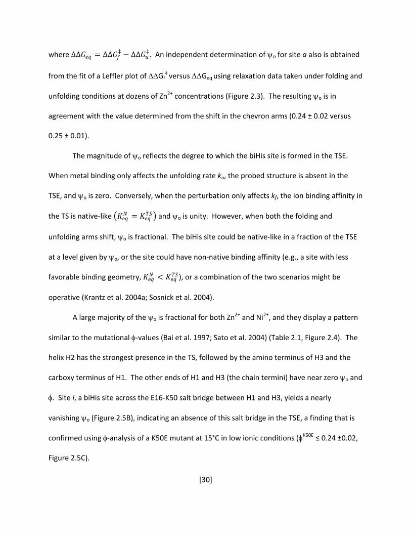
where ΔΔ𝐺𝐺𝑒𝑒𝑒𝑒 = ΔΔ𝐺𝐺𝑓𝑓‡ − ΔΔ𝐺𝐺𝑢𝑢
‡. An independent determination of ψo for site a also is obtained
from the fit of a Leffler plot of ∆∆Gf‡ versus ∆∆Geq using relaxation data taken under folding and
unfolding conditions at dozens of Zn2+ concentrations (Figure 2.3). The resulting ψo is in
agreement with the value determined from the shift in the chevron arms (0.24 ± 0.02 versus
0.25 ± 0.01).
The magnitude of ψo reflects the degree to which the biHis site is formed in the TSE.
When metal binding only affects the unfolding rate ku, the probed structure is absent in the
TSE, and ψo is zero. Conversely, when the perturbation only affects kf, the ion binding affinity in
the TS is native-like �𝐾𝐾𝑒𝑒𝑒𝑒𝑁𝑁 = 𝐾𝐾𝑒𝑒𝑒𝑒𝑇𝑇𝑇𝑇� and ψo is unity. However, when both the folding and
unfolding arms shift, ψo is fractional. The biHis site could be native-like in a fraction of the TSE
at a level given by ψo, or the site could have non-native binding affinity (e.g., a site with less
favorable binding geometry, 𝐾𝐾𝑒𝑒𝑒𝑒𝑁𝑁 < 𝐾𝐾𝑒𝑒𝑒𝑒𝑇𝑇𝑇𝑇 ), or a combination of the two scenarios might be
operative (Krantz et al. 2004a; Sosnick et al. 2004).
A large majority of the ψo is fractional for both Zn2+ and Ni2+, and they display a pattern
similar to the mutational φ-values (Bai et al. 1997; Sato et al. 2004) (Table 2.1, Figure 2.4). The
helix H2 has the strongest presence in the TS, followed by the amino terminus of H3 and the
carboxy terminus of H1. The other ends of H1 and H3 (the chain termini) have near zero ψo and
φ. Site i, a biHis site across the E16-K50 salt bridge between H1 and H3, yields a nearly
vanishing ψo (Figure 2.5B), indicating an absence of this salt bridge in the TSE, a finding that is
confirmed using φ-analysis of a K50E mutant at 15°C in low ionic conditions (φK50E ≤ 0.24 ±0.02,
Figure 2.5C).
[31]
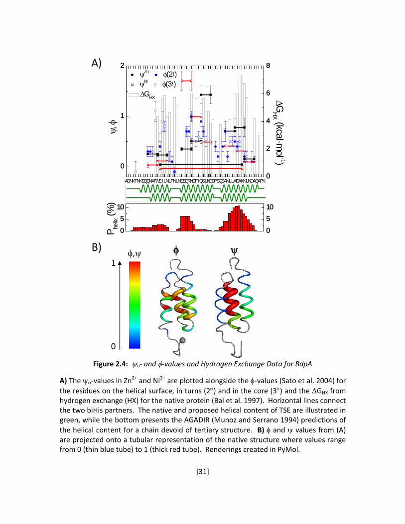
Figure 2.4: ψo- and φ-values and Hydrogen Exchange Data for BdpA
A) The ψο-values in Zn2+ and Ni2+ are plotted alongside the φ-values (Sato et al. 2004) for the residues on the helical surface, in turns (2°) and in the core (3°) and the ∆GHX from hydrogen exchange (HX) for the native protein (Bai et al. 1997). Horizontal lines connect the two biHis partners. The native and proposed helical content of TSE are illustrated in green, while the bottom presents the AGADIR (Munoz and Serrano 1994) predictions of the helical content for a chain devoid of tertiary structure. B) φ and ψ values from (A) are projected onto a tubular representation of the native structure where values range from 0 (thin blue tube) to 1 (thick red tube). Renderings created in PyMol.
ADNKFNKEQQNAFWEILNLPNLNEEQRNGFIQSLKDDPSQSANLLAEAKKLNDAQAPK0
2
4
6
8
∆GHX
0
1
2
∆GHX (kcal·m
ol -1)ψ,
φ
ψZn φ(2؛) ψNi φ(3؛)
0
5
10
0
5
10
P helix (%
)
A)
B)
φ,ψ
1
0
φ
ψ

[32]
Figure 2.5: Absence of the E16-K50 Salt Bridge Between H1-H3 Contacts According to ψ- and φ-
analysis A) The native E16-K50 salt bridge between H1- H3 is probed by separately inserting a biHis site (site i) and a K50E mutation. B) The biHis site is measured to be absent from the TS according to ψ-values taken in Zn2+ (□) and Ni2+ (). Multiphase behavior is observed in the presence of Ni2+; only the dominant phase is reported. Regardless, the metal has little effect on the TS. C) Similarly, a K50E substitution disrupts the salt bridge in the native state under low ionic conditions (50mM HEPES, urea rather than GdmCl) at 15°C. The φK50E
is calculated assuming the unfolding arms have the same slope (mu-value). Because of this assumption and the extrapolations involved, the φ-value at zero denaturant (0.24±0.02) should be considered an upper bound estimate. Overall, both methods indicate that E16-K50 contact is not well-formed in the TS.
1 2 3 4 5 6
1
2
3
4
RT ln
k obs (
kcal
·mol
-1)
[GdmCl] (M)
no metal 1mM Zn2+
1mM Ni2+
A)
B)
C)
3 4 5 6 7 82.0
2.5
3.0
3.5
4.0
4.5
RT ln
k obs (
kcal
·mol
-1)
[Urea] (M)
psWT K50E
[33]
2.3.2 Lack of TS Heterogeneity
The extensive number of fractional ψo-values for BdpA contrasts with the findings for Ub
(Krantz et al. 2004a), Acp (Pandit et al. 2006), and the cross-linked version of the GCN4 coiled
coil (Krantz and Sosnick 2001). These three proteins have clear TS nuclei containing multiple
native-like biHis sites whose ψo equal unity. In BdpA, the abundance of fractional ψ-values may
be indicative of structural heterogeneity in the TSE, as observed in the folding of the dimeric
version of the GCN4 coiled coil. Here, fractional ψo-values are observed along the length of the
coil. These values are due to TS heterogeneity wherein nucleation occurs at multiple sites
(Moran et al. 1999; Krantz and Sosnick 2001). The flux through each of these nuclei can be
manipulated by mutation, e.g. a destabilizing Ala→Gly mutation at one site decreased the
probability of nucleation occurring at this site, which increased the probability of nucleation at
other sites. The change in the probability of nucleation results in a change in the measured ψo-
values and provides a general strategy for investigating TS heterogeneity.
We use this strategy to investigate whether the TSE of BdpA is likewise heterogeneous.
The two most plausible competing TS structures would be the H1-H2 and H2-H3 microdomains,
the two most frequently predicted species (Itoh and Sasai 2006). Because the ψo- and φ-values
(Sato et al. 2004) generally are higher in the H2-H3 microdomain, this species should be the
more dominant. We sought to determine whether the population of the alternative species,
the H1-H2 microdomain, would increase in response to a destabilization of the H2-H3
microdomain. Accordingly, we introduce a L45A mutation at the H2-H3 interface, which is
known to destabilize the native state and the TS by 1.3 and 0.7 kcal·mol-1, respectively
(φL45A=0.5-0.6) (Sato et al. 2004). We test for an increase in the population of the H1-H2

[34]
microdomain by re-measuring the ψo-value for Site b, located at the carboxy terminus of H1, in
the background of the L45A substitution. This site spans the hydrophobic residues in the H1-H2
interface and is a representative site for the formation of this microdomain. In the
heterogeneous scenario, the degree of H2-H3 destabilization upon introduction of the L45A
mutation should increase the relative population of the minor H1-H2 species in the TS from
20% to at least 40%, according to the initial ψo-value for Site b (0.23 ± 0.03). However, ψo
remained unchanged (0.17 ± 0.02) (Figure 2.6A). This invariance after the significant
destabilization in H2-H3 is inconsistent with a heterogeneous TSE containing the H1-H2 and H2-
H3 microdomains as the major competing alternatives (Figure 2.6C). Therefore, we conclude
that the TSE is not composed of two distinct TS ensembles centered about H1-H2 or H2-H3
(Figure 2.6B), which is in agreement with recent work based on the temperature invariance of
φ-values (Sato and Fersht 2007).
Given this lack of TS heterogeneity, the origin of the fractional ψo can be understood by
their dependence on metal ion type. The different preferential coordination geometries of the
metal ions (Jia 1991) support the view that the fractional ψo emerge due to non-native binding
affinity in the TS, for example 𝐾𝐾𝑒𝑒𝑒𝑒𝑇𝑇𝑇𝑇 𝐾𝐾𝑒𝑒𝑒𝑒𝑁𝑁� ≈ 2 (Table 2.2). If the site has a distorted geometry in a
plastic TS, metals with different coordination geometries should stabilize the TS to different
extents, relative to the stability each metal imparts to the native state. Hence, the use of
different metal ions is likely to alter ψo, as observed in the present study. Overall, the
appearance of metal-dependent, non-unity ψo indicates that the biHis sites have a non-native
geometry in a malleable TS.
[35]
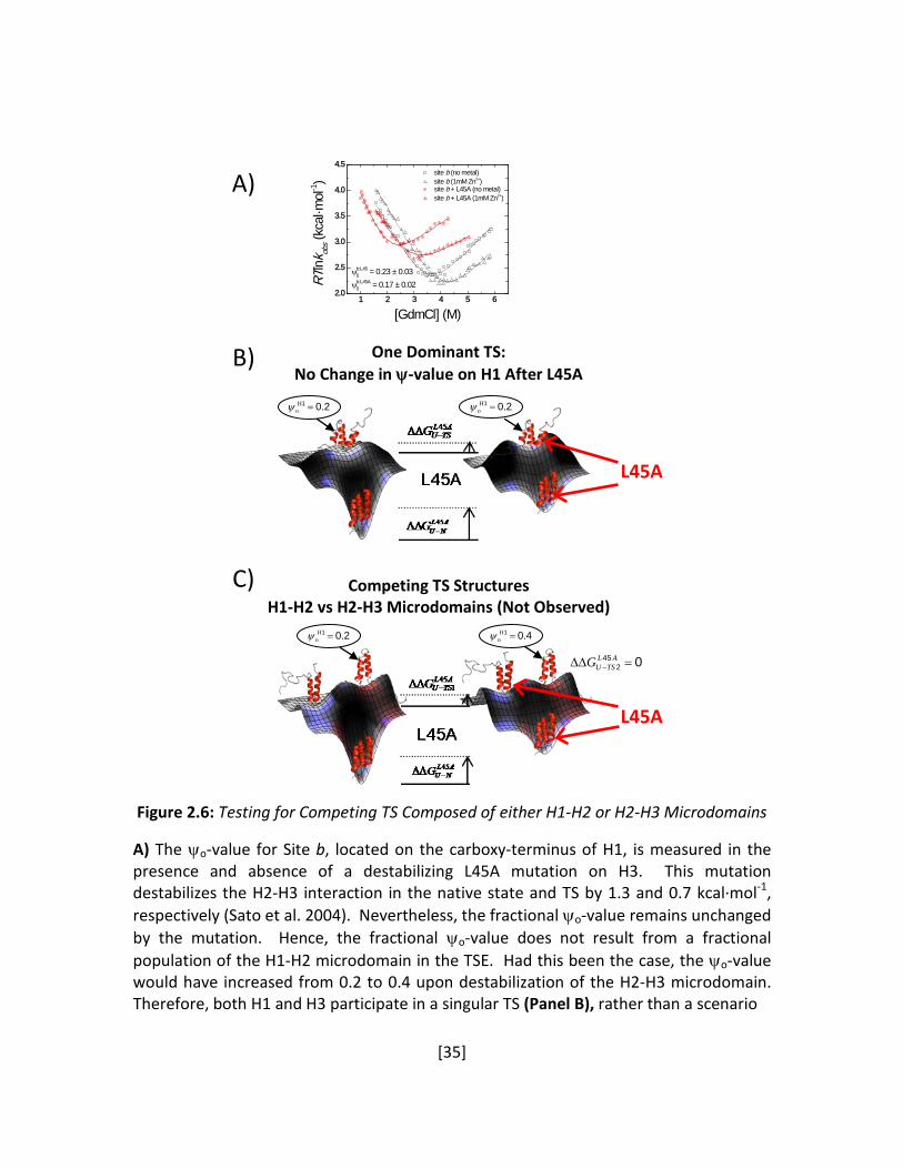
Figure 2.6: Testing for Competing TS Composed of either H1-H2 or H2-H3 Microdomains A) The ψo-value for Site b, located on the carboxy-terminus of H1, is measured in the presence and absence of a destabilizing L45A mutation on H3. This mutation destabilizes the H2-H3 interaction in the native state and TS by 1.3 and 0.7 kcal·mol-1, respectively (Sato et al. 2004). Nevertheless, the fractional ψo-value remains unchanged by the mutation. Hence, the fractional ψo-value does not result from a fractional population of the H1-H2 microdomain in the TSE. Had this been the case, the ψo-value would have increased from 0.2 to 0.4 upon destabilization of the H2-H3 microdomain. Therefore, both H1 and H3 participate in a singular TS (Panel B), rather than a scenario
1 2 3 4 5 62.0
2.5
3.0
3.5
4.0
4.5
RTln
k obs (
kcal
·mol
-1)
[GdmCl] (M)
site b (no metal) site b (1mM Zn2+) site b + L45A (no metal) site b + L45A (1mM Zn2+)
ψb:L450 = 0.23 ± 0.03
ψb:L45A0 = 0.17 ± 0.02
A)
B)
C)
One Dominant TS: No Change in ψ-value on H1 After L45A
Competing TS Structures H1-H2 vs H2-H3 Microdomains (Not Observed)
201 .Ho =ψ
201 .Ho =ψ 201 .H
o =ψ
401 .Ho =ψ
L45A
L45A
0452 =∆∆ −
ALTSUG

[36]
Figure 2.6 continued where the TS contains two competing populations composed of either the H1-H2 or the H2-H3 microdomains (Panel C).

[37]
Table 2.2: Relative Metal Binding Affinities in the U, N, and TSs
Site Mutationa ∆∆Geq (kinetic)
ψ0 𝐾𝐾𝑒𝑒𝑒𝑒𝑈𝑈 𝐾𝐾𝑒𝑒𝑒𝑒𝑁𝑁� 𝐾𝐾𝑒𝑒𝑒𝑒𝑇𝑇𝑇𝑇 𝐾𝐾𝑒𝑒𝑒𝑒𝑁𝑁� b Metal
a Q11H/Y15H
(H1)
0.71 ± 0.04 0.24 ± 0.02 3.6 ± 0.3 2.2 ± 0.2 Zn 0.79 ± 0.05c 0.25 ± 0.01c 4.3 ± 0.4c 2.4 ± 0.3c Znc
1.68 ± 0.10 0.039 ± 0.005 19.8 ± 3.5 11.5 ± 2.2 Ni
b Y15H/N19H
(H1) 0.81 ± 0.07 0.23 ± 0.03 4.2 ± 0.5 2.4 ± 0.4 Zn 1.40 ± 0.12 0.11 ± 0.02 12.1 ± 2.7 5.6 ± 1.4 Ni
c E25H/N29H
(H2) 1.19 ± 0.06 0.35 ± 0.03 8.2 ± 0.8 2.3 ± 0.3 Zn 0.77 ± 0.07 1.71 ± 0.19 4.0 ± 0.5 0.7 ± 0.1 Ni
d N29H/Q33H
(H2) 1.30 ± 0.08 0.51 ± 0.05 10.1 ± 1.4 1.8 ± 0.3 Zn 1.50 ± 0.04 0.99 ± 0.07 14.4 ± 1.3 1.0 ± 0.1 Ni
e Q33H/D37H
(H2) 0.28 ± 0.03 1.43 ± 0.18 1.7 ± 0.1 0.9 ± 0.1 Zn 1.28 ± 0.05 0.49 ± 0.04 9.6 ± 0.9 1.9 ± 0.2 Ni
f A43H/A47H
(H3) 0.47 ± 0.03 0.71 ± 0.06 2.3 ± 0.1 1.2 ± 0.1 Zn 1.16 ± 0.11 0.41 ± 0.04 7.8 ± 1.6 2.1 ± 0.5 Ni
g A47H/K51H
(H3) 0.59 ± 0.09 0.78 ± 0.18 2.8 ± 0.4 1.2 ± 0.3 Zn 1.53 ± 0.08 0.31 ± 0.02 15.1 ±2.1 2.8 ± 0.5 Ni
h K51H/A55H
(H3) 0.27 ± 0.11 0.15 ± 0.05 1.6 ± 0.3 1.5 ± 0.6 Zn 1.21 ± 0.10 0.09 ± 0.01 8.6 ± 1.5 5.1 ± 1.0 Ni
i E16H/K50H
(H1-H3) 1.68 ± 0.14 0.04 ± 0.01 19.8 ± 5.0 11.1 ± 3.1 Zn 1.69 ± 0.16d -0.04 ± 0.01d 20.0 ± 5.7d 64.5 ± 21.4 Ni
a Location of the biHis site is in parentheses.
b Determined by fitting ΔΔ𝐺𝐺𝑒𝑒𝑒𝑒Me2+assuming [Me2+] ≫ 𝐾𝐾𝑒𝑒𝑒𝑒𝑈𝑈 ,𝐾𝐾𝑒𝑒𝑒𝑒𝑁𝑁 .
c Values directly calculated from measuring folding and unfolding rates at fixed GdmCl concentrations of 2.4 M and 5.5 M, respectively, as a function of [Zn2+] (Figure 2.3B).

[38]
2.3.3 Amide H/D Kinetic Isotope Effect
To further characterize the TS, we determined the fraction of formed helical hydrogen
bonds (H-bonds) in the TS using backbone amide kinetic isotope effects (Kentsis and Sosnick
1998; Krantz et al. 2000; Krantz et al. 2002b). Folding rates of the protein with deuterated
amide hydrogens were compared to the protonated version for the same bulk solvent
conditions. The fraction 𝜙𝜙𝑓𝑓𝐷𝐷-𝐻𝐻 of formed helical H-bonds in the TS was obtained from the ratio
of the change in the folding activation free energy relative to the change in equilibrium stability,
i.e. 𝜙𝜙𝑓𝑓𝐷𝐷-𝐻𝐻 = ΔΔ𝐺𝐺𝑓𝑓
𝐷𝐷-𝐻𝐻 ΔΔ𝐺𝐺𝑒𝑒𝑒𝑒𝐷𝐷-𝐻𝐻� . We measured 𝜙𝜙𝑓𝑓
𝐷𝐷-𝐻𝐻 = 0.70 ± 0.02 from the difference in the
kinetic parameters obtained from the chevron plots of the deuterated and protonated proteins
in 11% D2O (Figure 2.7D). Also, the equilibrium isotope effect was determined from
independent equilibrium denaturation measurements (Figure 2.7A-C). The ΔΔ𝐺𝐺𝑒𝑒𝑒𝑒𝐷𝐷-𝐻𝐻 from the
equilibrium experiments agrees with the value obtained from the kinetic measurements (-0.39
± 0.03 versus -0.37 ± 0.06 kcal·mol-1).
The measured 𝜙𝜙𝑓𝑓𝐷𝐷-𝐻𝐻 indicates that ~70%, or ~23 of the 33 native helical hydrogen bonds
are formed in the TS. This percentage equates to the fraction of surface burial in the TS,
𝑚𝑚𝑓𝑓 𝑚𝑚0 = 0.72 ± 0.02⁄ , and is consistent with our proposal that roughly equal percentages of
tertiary and secondary structure are formed in the TS (Krantz et al. 2000; Krantz et al. 2002b).
A preliminarily interpretation is that 𝜙𝜙𝑓𝑓𝐷𝐷-𝐻𝐻 = 0.70 ± 0.02 indicates that 70% of the
native H-bonds are formed in the TS, but other possible interpretations of the kinetic isotope
data are now considered. All the H-bonds may be formed in the TSE, but with an average of
[39]
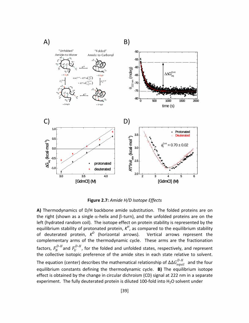
Figure 2.7: Amide H/D Isotope Effects
A) Thermodynamics of D/H backbone amide substitution. The folded proteins are on the right (shown as a single α-helix and β-turn), and the unfolded proteins are on the left (hydrated random coil). The isotope effect on protein stability is represented by the equilibrium stability of protonated protein, KH, as compared to the equilibrium stability of deuterated protein, KD (horizontal arrows). Vertical arrows represent the complementary arms of the thermodynamic cycle. These arms are the fractionation
factors, 𝐹𝐹𝑁𝑁𝐷𝐷-𝐻𝐻and 𝐹𝐹𝑈𝑈
𝐷𝐷-𝐻𝐻, for the folded and unfolded states, respectively, and represent the collective isotopic preference of the amide sites in each state relative to solvent.
The equation (center) describes the mathematical relationship of ΔΔ𝐺𝐺𝑒𝑒𝑒𝑒𝑢𝑢𝑒𝑒𝑒𝑒𝐷𝐷-𝐻𝐻 and the four
equilibrium constants defining the thermodynamic cycle. B) The equilibrium isotope effect is obtained by the change in circular dichroism (CD) signal at 222 nm in a separate experiment. The fully deuterated protein is diluted 100-fold into H2O solvent under
0 500 1000 1500 2000-80
-75
-70
-65
-60
-55
-50
θ 222
nm (m
deg)
time (s)
∆∆GD-Heq
3.0 3.5 4.0
-1.0
-0.5
0.0
0.5
1.0
∆Geq
(kca
l·mol
-1)
[GdmCl] (M)
protonated deuterated
2 3 4 5 62.0
2.5
3.0
3.5
RT ln
k obs (
kcal
·mol
-1)
[GdmCl] (M)
Protonated Deuterated
φD-Hf = 0.70 ± 0.02
A)
B)
C)
D)
[40]
Figure 2.7 continued conditions where stability is determined prior to significant backbone amide exchange (pH 4.5, 10°C)(Connelly et al. 1993). The stability of the deuterated and the protonated protein is determined from the initial and final CD levels. C) The equilibrium isotope effect is obtained at five different denaturant concentrations. The stability of the deuterated and the protonated protein are fit using the average mo-value obtained from the chevron data. D) In the kinetic isotope effect measurement, the different folding rates of protonated and deuterated proteins produce two offset chevrons. Their offset
translates to a 𝜙𝜙𝑓𝑓𝐷𝐷-𝐻𝐻 value of 0.70 ± 0.02, which equates to the fraction of backbone
amide helical hydrogen bonds formed in the TSE. The mf and mο for protonated (deuterated) state are 1.17 ± 0.03 (1.06 ± 0.02) and 1.64 ± 0.04 (1.54 ± 0.03) kcal·mol-1·M-1, respectively, and Δ𝐺𝐺𝑓𝑓
‡ = 3.22 ± 0.01 kcal·mol-1. The kinetic and equilibrium isotope
effects are ΔΔ𝐺𝐺𝑓𝑓‡ = -0.27 ± 0.02 kcal·mol-1 and ΔΔ𝐺𝐺𝑒𝑒𝑒𝑒𝑢𝑢𝑒𝑒𝑒𝑒
𝐷𝐷-𝐻𝐻 = -0.39 ± 0.03 kcal·mol-1. Values
for ∆∆Gf‡ and ∆∆Gu
‡ are calculated at 2.75 and 5.5 M GdmCl.
[41]
70% of the native isotope effect. A second possibility asserts that the 70% value might be due
to either all H-bonds either being formed 70% of the time, or being formed all of the time but in
a distorted geometry with 70% of the equilibrium isotope effect. Both possibilities are
inconsistent with the lack of helix formation at the amino and carboxy termini of H1 and H3,
respectively, as indicated by the near zero values for the φ and ψo across these regions (Figure
2.4).
The ensemble and time-averaged 70% isotope effect could also arise from intermediate
scenarios. For example, the entire TSE might have 60% of the H-bonds formed all of the time
and another 20% of the H-bonds formed half the time. In addition, the analysis of the kinetic
isotope effect assumes that all helical H-bonds contribute equally to the global ΔΔ𝐺𝐺𝑒𝑒𝑒𝑒𝐷𝐷-𝐻𝐻. This
assumption is supported by the linear scaling of ΔΔ𝐺𝐺𝑒𝑒𝑒𝑒𝐷𝐷-𝐻𝐻 with the total number of helical H-
bonds in the protein (Krantz et al. 2002b). Accordingly, we estimate that the percentage of H-
bonds may range from 60-80%. Our calculation below of the RCO of the TS accounts for these
possibilities.
The ~70% helical H-bond content of the TS reported by the analysis of 𝜙𝜙𝑓𝑓𝐷𝐷-𝐻𝐻 apparently
exceeds the fraction suggested by the ψo-values and the helix-probing φAla→Gly values (Sato et al.
2004). The kinetic isotope effect data provide a more definitive conclusion because H/D
substitution directly probes hydrogen bonding and only marginally perturbs the bonds. The low
ψo are likely to arise from distorted helical geometries in the TS. The φ-analysis only yields
definite conclusions regarding H2. Seven sites on the surface of H1 and H3 have φAla→Gly
between 0.3-0.5. Four of these sites have ΔΔ𝐺𝐺𝑒𝑒𝑒𝑒Ala→Gly ~1.5-1.8 kcal·mol-1, which is about 1
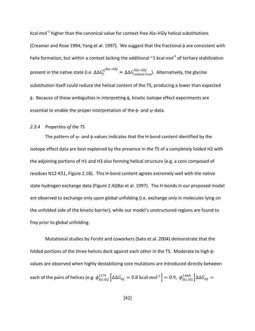
[42]
kcal·mol-1 higher than the canonical value for context-free Ala→Gly helical substitutions
(Creamer and Rose 1994; Yang et al. 1997). We suggest that the fractional φ are consistent with
helix formation, but within a context lacking the additional ~1 kcal·mol-1 of tertiary stabilization
present in the native state (i.e. ΔΔ𝐺𝐺𝑓𝑓‡Ala→Gly
≈ ΔΔ𝐺𝐺context freeAla→Gly ). Alternatively, the glycine
substitution itself could reduce the helical content of the TS, producing a lower than expected
φ. Because of these ambiguities in interpreting φ, kinetic isotope effect experiments are
essential to enable the proper interpretation of the φ- and ψ-data.
2.3.4 Properties of the TS
The pattern of ψ- and φ-values indicates that the H-bond content identified by the
isotope effect data are best explained by the presence in the TS of a completely folded H2 with
the adjoining portions of H1 and H3 also forming helical structure (e.g. a core composed of
residues N12-K51, Figure 2.1B). This H-bond content agrees extremely well with the native
state hydrogen exchange data (Figure 2.4)(Bai et al. 1997). The H-bonds in our proposed model
are observed to exchange only upon global unfolding (i.e. exchange only in molecules lying on
the unfolded side of the kinetic barrier), while our model’s unstructured regions are found to
fray prior to global unfolding.
Mutational studies by Fersht and coworkers (Sato et al. 2004) demonstrate that the
folded portions of the three helices dock against each other in the TS. Moderate to high φ-
values are observed when highly destabilizing core mutations are introduced directly between
each of the pairs of helices (e.g. 𝜙𝜙H1-H2I17V �ΔΔ𝐺𝐺𝑒𝑒𝑒𝑒 = 0.8 kcal·mol-1� = 0.9, 𝜙𝜙H1-H3
L46A �ΔΔ𝐺𝐺𝑒𝑒𝑒𝑒 =
[43]
1.9 kcal·mol-1� = 0.5, 𝜙𝜙H2-H3L45A �ΔΔ𝐺𝐺𝑒𝑒𝑒𝑒 = 1.5 kcal·mol-1� = 0.5) as well as in the core between
the three helices (e.g. 𝜙𝜙H1-H2-H3L35A �ΔΔ𝐺𝐺𝑒𝑒𝑒𝑒 = 2.4 kcal·mol-1� = 0.5, 𝜙𝜙H1-H2-H3
A49G �ΔΔ𝐺𝐺𝑒𝑒𝑒𝑒 =
3.6 kcal·mol-1� = 0.5). Given these results, the TS can be described as a mini-three helix
bundle with frayed termini.
A TS model containing 70% of the formed H-bonds produces an RCOTS/RCON ratio of
0.66-0.72, depending on the exact location of the native-like helical H-bond and assuming that
the remaining regions are unstructured. To test the robustness of this fraction, the RCOTS is
recalculated for models having 60-80% of the H-bonds formed. The calculated RCO ratios range
from 0.61 – 0.72 when assuming a native-like geometry for the folded regions, as suggested by
the high inter-helical φ-values. The next section analyzes this assumption and the influence of
chain relaxation in the TSE on the RCOTS/RCON fraction.
2.3.5 Relaxing the TS model
All-atom implicit solvent Langevin dynamics (LD) simulations (Shen and Freed 2002b; a)
are employed to investigate potential structural relaxation of the native-like TS models and the
effect on their RCO values (Figure 2.8, Figure 2.9). This modeling is motivated by the mounting
evidence that proteins undergo some chain relaxation along the folding trajectory, for example,
minimizing energy through the formation of non-native hydrophobic interactions as observed
in the intermediates of Rd-apocytochrome b562 (Feng et al. 2004), IM7 (Capaldi et al. 2002), and
apomyoglobin (Nishimura et al. 2006), and in the TS of Ub (Sosnick et al. 2004). Specifically, the
turns in BdpA between the helices yield low φ-values (Sato et al. 2004), indicating that the
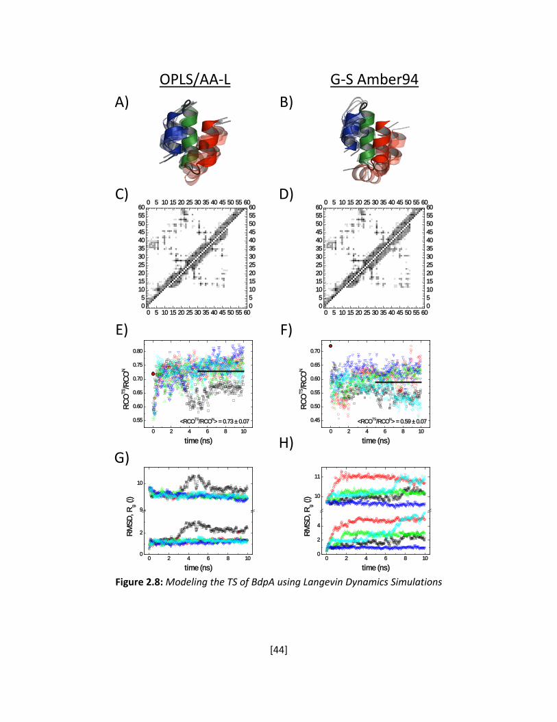
[44]
Figure 2.8: Modeling the TS of BdpA using Langevin Dynamics Simulations
0 5 10 15 20 25 30 35 40 45 50 55 6005
1015202530354045505560
0 5 10 15 20 25 30 35 40 45 50 55 60
051015202530354045505560
0 2 4 6 8 10
0.55
0.60
0.65
0.70
0.75
0.80
RCO
TS/R
CON
time (ns)
<RCOTS/RCON> = 0.73 ± 0.07
0 5 10 15 20 25 30 35 40 45 50 55 6005
1015202530354045505560
0 5 10 15 20 25 30 35 40 45 50 55 60
051015202530354045505560
0 2 4 6 8 10
0.45
0.50
0.55
0.60
0.65
0.70
RCO
TS/R
CON
time (ns)
<RCOTS/RCON> = 0.59 ± 0.07
0 2 4 6 8 100
2
9
10
RMSD
, Rg ((إ
time (ns)0 2 4 6 8 10
0
2
4
10
11
RMSD
, Rg ((إ
time (ns)
A)
B)
C)
D)
E)
F)
G)
H)
OPLS/AA-L
G-S Amber94
[45]
Figure 2.8 continued Our initial model of the TS has native-like residues N12-K51 (black), representing 70% helical hydrogen bond formation. It is superimposed on representative structures taken from ten LD simulations using either the OPLS/AA-L (Panel A) or G-S Amber 94 force field (Panel B). The native helical residues for H1, H2, and H3 are colored blue, green, and red, respectively. Unstructured regions are not shown for clarity and are assumed to make no additional contacts. Average contact maps are calculated for five separate simulations (in different colors) from the structures appearing in the last 5 ns and are presented in the lower diagonals of Panels C-D, while the average contact map from the NMR ensemble (26 structures)(Sato et al. 2004) are shown in the upper diagonals. Despite the increased motion of H3 in the G-S Amber 94 force field in D, the average contact map still exhibits native-like behavior with H1-H3 contacts. In the RCO plots (Panels E-F), the RCOTS/RCON of the initial structural model is shown ( ) along with the average value from the last 5 ns (solid line) of the trajectories. Changes in RMSD and Rg (Panels G-H) track with the observed changes in RCO. Renderings created in PyMol.

[46]
A) N12-E48: 60% H-BondsG-S Amber94
0 5 10 15 20 25 30 35 40 45 50 55 6005
1015202530354045505560
0 5 10 15 20 25 30 35 40 45 50 55 60
051015202530354045505560
0 2 4 6 8 10
0.45
0.50
0.55
0.60
0.65
RCO
TS/R
CON
time (ns)
<RCOTS/RCON> = 0.57 ± 0.070 2 4 6 8 10
0
2
4
9
10
11
RMSD
,Rg (
Å)
time (ns)
0 5 10 15 20 25 30 35 40 45 50 55 6005
1015202530354045505560
0 5 10 15 20 25 30 35 40 45 50 55 60
051015202530354045505560
0 2 4 6 8 100
2
9
10
RMSD
, Rg (
Å)
time (ns)0 2 4 6 8 10
0.50
0.55
0.60
0.65
0.70
0.75
<RCOTS/RCON> = 0.66 ± 0.06
RC
OTS
/RCO
N
time (ns)
B) N7-A49: 80% H-Bonds
OPLS/AA-L G-S Amber94
0 5 10 15 20 25 30 35 40 45 50 55 6005
1015202530354045505560
0 5 10 15 20 25 30 35 40 45 50 55 60
051015202530354045505560
0 2 4 6 8 100.45
0.50
0.55
0.60
0.65
0.70
0.75
<RCOTS/RCON> = 0.64 ± 0.07
RCO
TS/R
CON
time (ns)0 2 4 6 8 10
0
2
4
10
11
RMSD
, Rg (
Å)
time (ns)
0 5 10 15 20 25 30 35 40 45 50 55 6005
1015202530354045505560
0 5 10 15 20 25 30 35 40 45 50 55 60
051015202530354045505560
0 2 4 6 8 10
0.50
0.55
0.60
0.65
0.70
0.75
0.80
<RCOTS/RCON> = 0.68 ± 0.07
RCO
TS/R
CON
time (ns)0 2 4 6 8 10
0
2
4
6
10
11
RMSD
, Rg (
Å)
time (ns)
OPLS/AA-L
Figure 2.9: Modeling the TS of BdpA with Different Fractions of Native H-bonds
The results of LD simulations using two different force fields are shown for two other models each with a subset of helical residues corresponding to different hydrogen bond percentages: Panel A, Residues N12-E48 (60%); Panel B, Residues N7-E49 (80%). The initial TS model is obtained by adding an extra hydrogen bond term for the subset of residues identified to be helical by the isotope effect data and by truncating the unstructured regions. In each panel, representative structures from LD simulations with the corresponding force field are superimposed (transparent) on the initial structure (solid). The native helical residues for H1, H2, and H3 are colored blue, green, and red, respectively. Both H3, and to a lesser degree H1, move relative to H2. The unstructured termini are not shown for clarity. The lower diagonal of each map displays the average contact map for the TS core from the last 5 ns of the five simulations. The average
[47]
Figure 2.9 continued contact map of the native NMR ensemble (containing 26 structures, 1SS1(Sato et al. 2004)) is presented in the upper diagonal. Significant changes in the radius of gyration, Rg, and RMSD are also reflected in appropriate changes in the RCO. Renderings created in PyMol. The RCOTS/RCON of the initial structural model is shown ( ) along with the average value from 5 – 10 ns (solid line).

[48]
helices repack, being shifted or rotated relative to their native positions. Furthermore, the
intermediate ψ-values reveal a level of plasticity in the TS in BpdA. Additional evidence for TS
relaxation of BdpA is the preferential stabilization of the TS for G30 mutations (Arora et al.
2004; Dimitriadis et al. 2004; Sato and Fersht 2007).
The robustness of the theoretical predictions is tested by running separate implicit
solvent LD simulations employing two different force fields, OPLS/AA-L (Kaminski et al. 2000;
2001) and Garcia and Sanbonmatsu’s modified version of Amber 94 (G-S Amber 94)(Garcia and
Sanbonmatsu 2002). Beyond the standard terms in the force fields, the only additional
constraints posited are for the H-bonds in the TSE. The O – H distances in these H-bonds are
constrained to the native distances using a harmonic force constant of 100 kcal·mol-1·Å-1. The
goal is to generate models of the TSE that are consistent with the experimental data rather
than predict or test whether the model is a true transition state. Accordingly, simulations are
conducted using only the folded residues (e.g. N12-K51) to avoid obtaining a trajectory that
follows a possible downhill reaction towards the N or U states.
Figure 2.8 displays the results of two sets of five 10 ns trajectories for a mini-bundle of
N12-K51 starting with 70% H-bond formation (five trajectories per force field). Trajectories
with either force field indicate that the imposed O – H distance restraints provide enough
stability that the three helices remain folded and in a native-like topology, although the
structures do rearrange occasionally. Without the H-bond restraints, the three helices unfold
and dissociate (data not shown).
[49]
During the initial 2 ns portion of the trajectories, H1 and H3 reposition themselves
relative to the largely unperturbed H2. The three helices remain mostly in contact although H3
exhibits a low level of undocking with the G-S Amber94 force field (compare Figure 2.8 A and
B). Regardless, the average contact map over the last 5ns of the trajectories still retains the
native pattern (Figure 2.8C, D). Because of the increased freedom of motion for H3, the
structures calculated using the G-S Amber94 force field retain a smaller fraction of the native
RCO, ⟨RCO𝑇𝑇𝑇𝑇 RCO𝑁𝑁⁄ ⟩5 trajectories5-10 ns = 59 ± 7% (Figure 2.8F). The corresponding OPLS/AA-L
trajectories predict the RCO as remaining much closer to the initial value,
⟨RCO𝑇𝑇𝑇𝑇 RCO𝑁𝑁⁄ ⟩5 trajectories5-10 ns = 73 ± 7% (Figure 2.8E). Very similar conclusions are obtained for
models where the simulations begin with constraints applied for either 60% or 80% of the
native helical H-bond content (Figure 2.9).
In summary, the LD simulations indicate that the RCOTS/RCON ratio of 0.6-0.7 from our
TS models is robust to the chain relaxation occurring in LD as well as to the modification in the
assumed degree of helical H-bond content in the TSE.
2.4 Discussion
The TS ensemble of BdpA is well-described as a mini three-helix bundle with frayed
ends. This identification has been determined using a combination of ψ- and φ-analysis and
kinetic isotope data. Beginning from this TS mini-bundle, folding to the native state proceeds
by the extension of the two terminal helices and potentially by a mild readjustment of their
relative orientation. The RCO for the TS varies between 60-70% of the native value, with the
uncertainty representing the extent of H-bonding and the degree of structural relaxation.
[50]
The folding of small proteins has been proposed by us (Sosnick et al. 1995; Sosnick et al.
1996; Englander et al. 1998) and others (Abkevich et al. 1994; Guo and Thirumalai 1995) to be a
nucleation process with the chain attaining a coarse version of the native topology in the TS.
This proposal is supported by the well known correlation between ln kf and the RCO, a metric
of topological complexity (Plaxco et al. 1998). For three proteins, BdpA, Ub, and Acp, whose
topologies span the observed range of RCO values, we have shown that their TSEs share a
common and high fraction of the native topology, RCOTS ≈ 0.7∙RCON. Accordingly, we contend
that the TSEs of other proteins satisfying the RCO correlation should also exhibit RCOs sharing
this high fraction.
As further support of our contention, Wallin and Chan use a Cα Gō-like model and find
the TSEs of 13 proteins have 0.7·RCON (Wallin and Chan 2006). Similarly, all-atom simulations
by Vendruscolo et al. for ten proteins find TSEs that share a common, albeit lower fraction,
0.5·RCON (Paci et al. 2005), potentially due to the incorporation of φ-values in the analysis that
may underestimate chain-chain contacts. Likewise, Bai, Zhou and Zhou find that the use of a
universal 78% value for the Total Contact Distance of the TS produces the best correlation
between the critical nucleation size of the TS and ln kf for 41 proteins (Bai et al. 2004).
We utilize the RCO metric to characterize a protein’s topology, in part, because of its
broad usage. Other metrics (Goldenberg 1999; Ivankov et al. 2003; Bai et al. 2004) produce a
similar conclusion. An advantage of the RCO metric is that topologically similar TS structures
provide similar RCO values even when there is local “microscopic heterogeneity”, such as
frayed helices or hairpins (Pandit et al. 2006), because the frayed portions in the simulations
[51]
have contacts with approximately the same average sequence separation as their neighbors.
Hence, the RCO, which is normalized to the number of contacts, remains unchanged upon
fraying.
However, all such metrics are just proxies for the key properties of the TS. Any single
parameter is likely to be insufficient to characterize a diverse set of protein folds. At the TS, the
addition of more native-like structure pushes the system thermodynamically downhill. The
chain is already pinned at enough points in the TS that further structure formation is
thermodynamically favorable. The precise RCO at which this situation ensues varies according
to the type and arrangement of secondary structure elements in any individual protein.
Nevertheless, our results indicate that a native-like topology is expected to be a general
property of the TS for many proteins.
2.5 Implications
The RCOTS ~ 0.7·RCON relationship provides a useful guide for interpreting previous
studies and for modeling the TSs of other proteins. For example, a high RCOTS/RCON fraction
restricts the degree to which a TS can be small and polarized, as has been inferred from φ-data
for some proteins that obey the RCO correlation (Grantcharova et al. 1998; Gruebele and
Wolynes 1998; Riddle et al. 1999; Klimov and Thirumalai 2001; Lindberg et al. 2002; Weikl and
Dill 2003; Yi et al. 2003; Garcia-Mira et al. 2004; Guo et al. 2004). Using the published φ-values,
we estimate that RCOTS < 0.5·RCON, although the precise number depends on the threshold for
which a φ-value is considered to be a contact. It seems unlikely that a universal RCO correlation
would hold if some proteins have a small polarized TS containing only local structure and a low
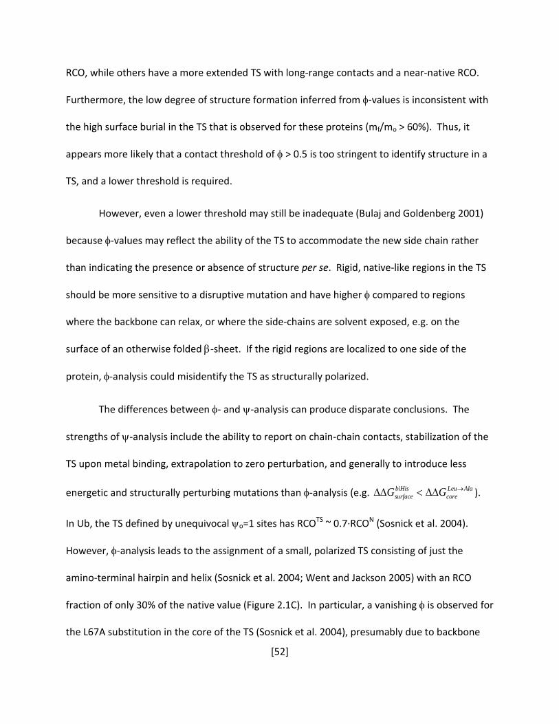
[52]
RCO, while others have a more extended TS with long-range contacts and a near-native RCO.
Furthermore, the low degree of structure formation inferred from φ-values is inconsistent with
the high surface burial in the TS that is observed for these proteins (mf/mo > 60%). Thus, it
appears more likely that a contact threshold of φ > 0.5 is too stringent to identify structure in a
TS, and a lower threshold is required.
However, even a lower threshold may still be inadequate (Bulaj and Goldenberg 2001)
because φ-values may reflect the ability of the TS to accommodate the new side chain rather
than indicating the presence or absence of structure per se. Rigid, native-like regions in the TS
should be more sensitive to a disruptive mutation and have higher φ compared to regions
where the backbone can relax, or where the side-chains are solvent exposed, e.g. on the
surface of an otherwise folded β-sheet. If the rigid regions are localized to one side of the
protein, φ-analysis could misidentify the TS as structurally polarized.
The differences between φ- and ψ-analysis can produce disparate conclusions. The
strengths of ψ-analysis include the ability to report on chain-chain contacts, stabilization of the
TS upon metal binding, extrapolation to zero perturbation, and generally to introduce less
energetic and structurally perturbing mutations than φ-analysis (e.g. AlaLeucore
biHissurface GG →∆∆<∆∆ ).
In Ub, the TS defined by unequivocal ψo=1 sites has RCOTS ~ 0.7·RCON (Sosnick et al. 2004).
However, φ-analysis leads to the assignment of a small, polarized TS consisting of just the
amino-terminal hairpin and helix (Sosnick et al. 2004; Went and Jackson 2005) with an RCO
fraction of only 30% of the native value (Figure 2.1C). In particular, a vanishing φ is observed for
the L67A substitution in the core of the TS (Sosnick et al. 2004), presumably due to backbone
[53]
readjustment or side chain exposure. These possibilities are not as likely in the core of the
hairpin-helix motif where higher φ are observed.
Our conclusion that φ-analysis underestimates the structural content of Ub’s TS is
likewise consistent with Bulaj and Goldenberg’s findings of low φ in regions of native-like
structure in BPTI intermediates (Bulaj and Goldenberg 2001). These concerns should be
considered in the calculation of φ from folding simulations and in the interpretation of
experimental data where a small, polarized TS has been identified. For example, high φ-values
are located only on a single hairpin for Protein G (McCallister et al. 2000; Nauli et al. 2001) and
Protein L (Kim et al. 2000). As noted by the authors, the participation of a third strand adjacent
to the dominant hairpin in Protein G is suggested by three φ-values close to 0.4 (McCallister et
al. 2000). Analogously in Protein L, two φ-values close to 0.3 suggest some interaction of a third
strand and helix in the TSE (Kim et al. 2000).
The Protein G and Protein L results highlight the inherent difficulty in defining
thresholds for φ that are suitable to infer the presence of structure in the TS. With only a
hairpin, and even part of the helix, these models for the TS would predict a RCO fraction of only
~40%. Our RCOTS ~ 0.7·RCON relationship requires that the TSEs of Proteins G and L include
these additional long-range contacts, minimally with the adjoining β-strand, and potentially
some docked (Kim et al. 1998; McCallister et al. 2000) helical structure (Krantz et al. 2002b).
Such a configuration would produce a RCO ratio of ~80% (Figure 2.10). Using these principles, a
possible TS for srcSH3 is also created with an RCO in excess of 60%, by taking advantage of
known information for φ (Northey et al. 2002a), ψo (Shandiz et al. 2007), and mf/mo.
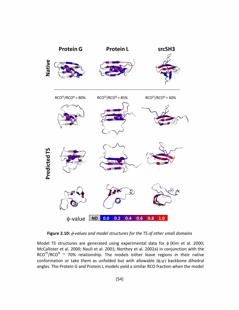
[54]
RCOTS/RCON = 80% RCOTS/RCON = 85% RCOTS/RCON = 60%
Protein G Protein L srcSH3N
ativ
ePr
edic
ted
TS
φ-value 0.0 0.2 0.4 0.6 0.8ND 1.0
Figure 2.10: φ-values and model structures for the TS of other small domains
Model TS structures are generated using experimental data for φ (Kim et al. 2000; McCallister et al. 2000; Nauli et al. 2001; Northey et al. 2002a) in conjunction with the RCOTS/RCON ~ 70% relationship. The models either leave regions in their native conformation or take them as unfolded but with allowable (φ,ψ) backbone dihedral angles. The Protein G and Protein L models yield a similar RCO fraction when the model

[55]
Figure 2.10 continued lacks the helix. Kinetic isotope studies (Krantz et al. 2002b) and φ-values for positions on the sole helix’s hydrophobic face indicate some helical presence in the TS. A TS for srcSH3 is constructed using φ-values (Northey et al. 2002a) and ψ-analysis (Shandiz et al. 2007). Renderings created in PyMol.
[56]
2.5.1 TS and Pathway Diversity
The high degree of native topology in the TS implied by the RCOTS~0.7·RCON relationship
greatly limits the degree of TS heterogeneity. Experimentally, minimal evidence exists for TS
heterogeneity as defined by the participation of different subsets of helices or strands
(Wright et al. 2003; Krantz et al. 2004a; Pandit et al. 2006) (rather than local “microscopic
heterogeneity” (Pandit et al. 2006) such as frayed helices or hairpins).
Even when the TS is homogenous, the pathway to and from the TS could be diverse.
However, a growing body of data indicates that elements of secondary structures, or “foldons”,
form in a well-defined sequence after crossing the initial rate-limiting barrier to collapse
(Krishna and Englander 2007). This scenario is due to chain connectivity and sequential
stabilization wherein pre-existing structures provide a foundation on which unfolded regions
can dock. For many proteins, the addition of foldons after the TS only can be accomplished, or
is strongly preferred, in a specific order due to the presence of a structural hierarchy.
On the way up to the TS from the denatured state, the issue is less clear. A multitude of
unstable conformations are sampled, but some structures provide a more suitable base for the
addition of other elements. Accordingly the uphill steps should involve a largely sequential
accretion of structure (Krantz et al. 2004a), although the energetic biases may not be as
pronounced as for the post-TS pathways.
Since smaller proteins such as BdpA have TSs with less structural hierarchy, they can
exhibit more pathway diversity. Furthermore, the symmetry of BdpA permits independent
association of H1 or H3 with H2. Hence, the path to the TS may begin with the formation of
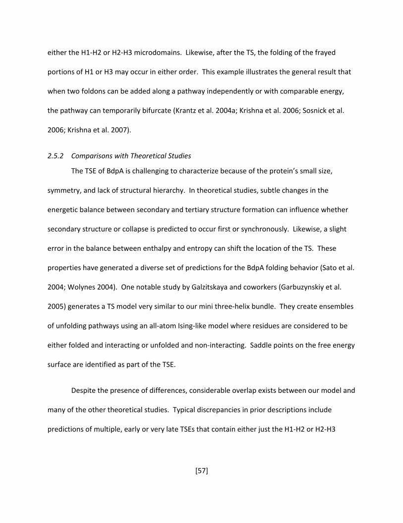
[57]
either the H1-H2 or H2-H3 microdomains. Likewise, after the TS, the folding of the frayed
portions of H1 or H3 may occur in either order. This example illustrates the general result that
when two foldons can be added along a pathway independently or with comparable energy,
the pathway can temporarily bifurcate (Krantz et al. 2004a; Krishna et al. 2006; Sosnick et al.
2006; Krishna et al. 2007).
2.5.2 Comparisons with Theoretical Studies
The TSE of BdpA is challenging to characterize because of the protein’s small size,
symmetry, and lack of structural hierarchy. In theoretical studies, subtle changes in the
energetic balance between secondary and tertiary structure formation can influence whether
secondary structure or collapse is predicted to occur first or synchronously. Likewise, a slight
error in the balance between enthalpy and entropy can shift the location of the TS. These
properties have generated a diverse set of predictions for the BdpA folding behavior (Sato et al.
2004; Wolynes 2004). One notable study by Galzitskaya and coworkers (Garbuzynskiy et al.
2005) generates a TS model very similar to our mini three-helix bundle. They create ensembles
of unfolding pathways using an all-atom Ising-like model where residues are considered to be
either folded and interacting or unfolded and non-interacting. Saddle points on the free energy
surface are identified as part of the TSE.
Despite the presence of differences, considerable overlap exists between our model and
many of the other theoretical studies. Typical discrepancies in prior descriptions include
predictions of multiple, early or very late TSEs that contain either just the H1-H2 or H2-H3
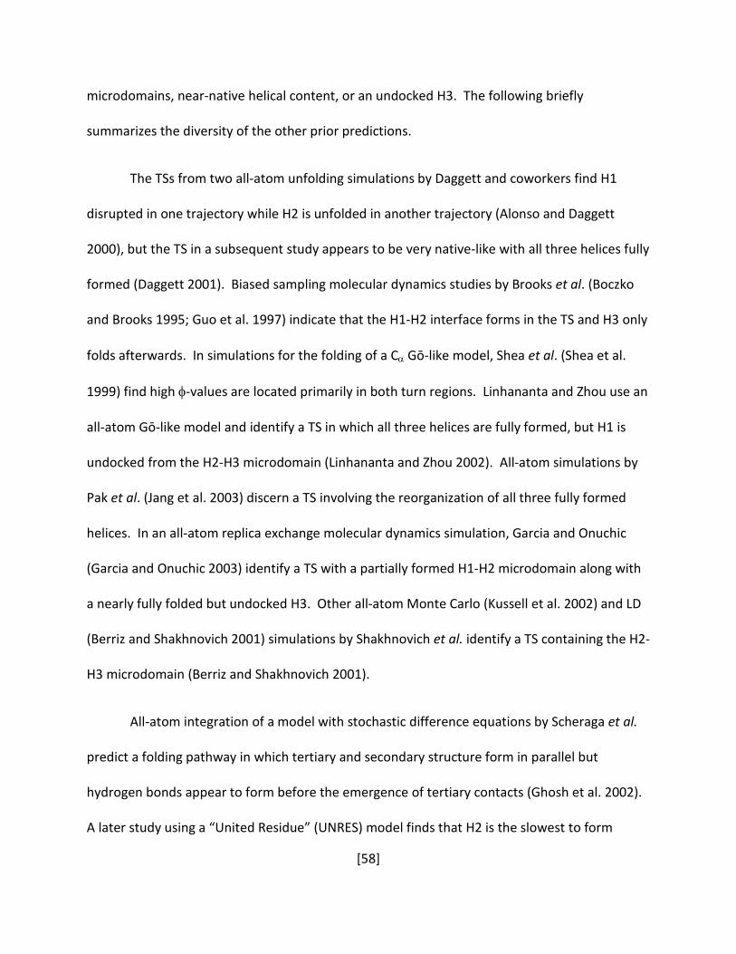
[58]
microdomains, near-native helical content, or an undocked H3. The following briefly
summarizes the diversity of the other prior predictions.
The TSs from two all-atom unfolding simulations by Daggett and coworkers find H1
disrupted in one trajectory while H2 is unfolded in another trajectory (Alonso and Daggett
2000), but the TS in a subsequent study appears to be very native-like with all three helices fully
formed (Daggett 2001). Biased sampling molecular dynamics studies by Brooks et al. (Boczko
and Brooks 1995; Guo et al. 1997) indicate that the H1-H2 interface forms in the TS and H3 only
folds afterwards. In simulations for the folding of a Cα Gō-like model, Shea et al. (Shea et al.
1999) find high φ-values are located primarily in both turn regions. Linhananta and Zhou use an
all-atom Gō-like model and identify a TS in which all three helices are fully formed, but H1 is
undocked from the H2-H3 microdomain (Linhananta and Zhou 2002). All-atom simulations by
Pak et al. (Jang et al. 2003) discern a TS involving the reorganization of all three fully formed
helices. In an all-atom replica exchange molecular dynamics simulation, Garcia and Onuchic
(Garcia and Onuchic 2003) identify a TS with a partially formed H1-H2 microdomain along with
a nearly fully folded but undocked H3. Other all-atom Monte Carlo (Kussell et al. 2002) and LD
(Berriz and Shakhnovich 2001) simulations by Shakhnovich et al. identify a TS containing the H2-
H3 microdomain (Berriz and Shakhnovich 2001).
All-atom integration of a model with stochastic difference equations by Scheraga et al.
predict a folding pathway in which tertiary and secondary structure form in parallel but
hydrogen bonds appear to form before the emergence of tertiary contacts (Ghosh et al. 2002).
A later study using a “United Residue” (UNRES) model finds that H2 is the slowest to form
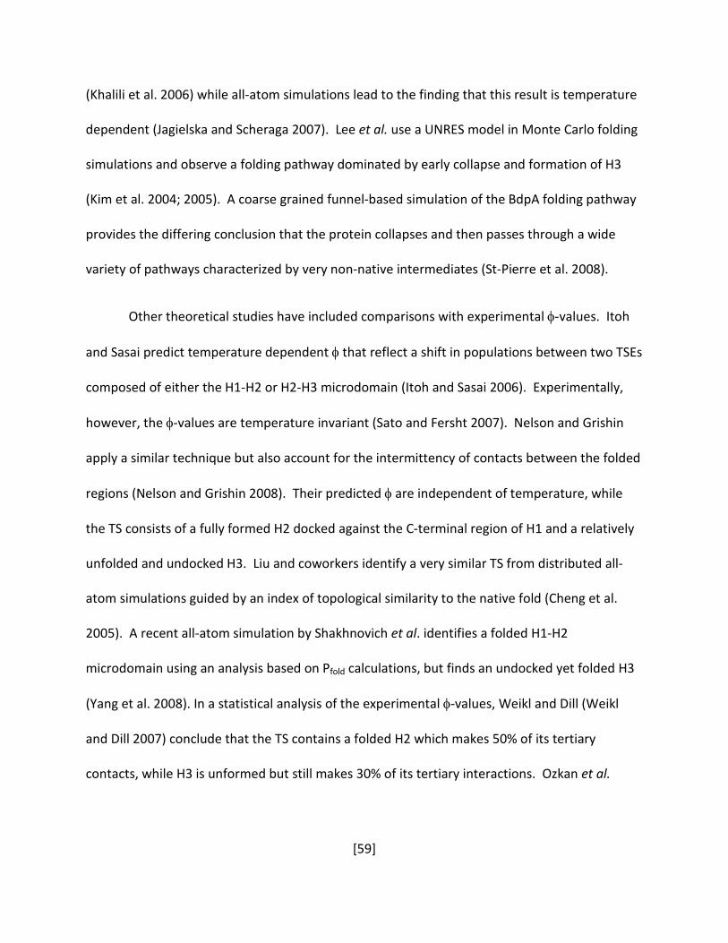
[59]
(Khalili et al. 2006) while all-atom simulations lead to the finding that this result is temperature
dependent (Jagielska and Scheraga 2007). Lee et al. use a UNRES model in Monte Carlo folding
simulations and observe a folding pathway dominated by early collapse and formation of H3
(Kim et al. 2004; 2005). A coarse grained funnel-based simulation of the BdpA folding pathway
provides the differing conclusion that the protein collapses and then passes through a wide
variety of pathways characterized by very non-native intermediates (St-Pierre et al. 2008).
Other theoretical studies have included comparisons with experimental φ-values. Itoh
and Sasai predict temperature dependent φ that reflect a shift in populations between two TSEs
composed of either the H1-H2 or H2-H3 microdomain (Itoh and Sasai 2006). Experimentally,
however, the φ-values are temperature invariant (Sato and Fersht 2007). Nelson and Grishin
apply a similar technique but also account for the intermittency of contacts between the folded
regions (Nelson and Grishin 2008). Their predicted φ are independent of temperature, while
the TS consists of a fully formed H2 docked against the C-terminal region of H1 and a relatively
unfolded and undocked H3. Liu and coworkers identify a very similar TS from distributed all-
atom simulations guided by an index of topological similarity to the native fold (Cheng et al.
2005). A recent all-atom simulation by Shakhnovich et al. identifies a folded H1-H2
microdomain using an analysis based on Pfold calculations, but finds an undocked yet folded H3
(Yang et al. 2008). In a statistical analysis of the experimental φ-values, Weikl and Dill (Weikl
and Dill 2007) conclude that the TS contains a folded H2 which makes 50% of its tertiary
contacts, while H3 is unformed but still makes 30% of its tertiary interactions. Ozkan et al.

[60]
describe the folding of BdpA using a zipping and assembly method and observe the formation
of the H2-H3 microdomain followed by the docking of H1 (Ozkan et al. 2007).
Diffusion-collision (DC) mechanisms, introduced either by assuming that folding is
limited by the collision of pre-formed helices (Myers and Oas 2001; Islam et al. 2002) or when
this behavior is observed in simulations (Zhou and Karplus 1999; Linhananta et al. 2002; Jang et
al. 2003; Jayachandran et al. 2007), predict that the H2-H3 microdomain plays the primary role
because these two helices have the highest intrinsic helicity (Figure 2.3). Although frequently
cited as supporting evidence, the observation of helical content in the TS is insufficient to
determine whether the structure forms before or after chain collision. A rare direct test of the
DC model demonstrates that helix formation occurs after initial chain collision for a coiled coil
that is engineered to have negligible intrinsic helicity (Meisner and Sosnick 2004). Although it is
difficult to falsify the DC model, we note that the structural content of the BdpA TS does not
follow the pattern predicted by intrinsic helicity (e.g. H3 is unstructured at the carboxy
terminus, although this half of the helix has higher intrinsic helicity than the folded regions of
H1).
2.6 Conclusion
The small size and symmetry of BdpA makes it an attractive model system. Rather than
simplifying the situation, however, these features along with minimal structural hierarchy
render the determination of the TS particularly challenging. Nevertheless, we have
characterized the TS using a combination of methods.

[61]
A goal of the present study is to quantify the topological requirements of the TS. Our TS
model for BdpA has an RCO that is ~ 60-80% of that for the native state. In conjunction with
similar results for two more complex α/β proteins, Ub and Acp, we propose that the proteins
satisfying the RCO correlation also have a TS that adopts 60-80% of the native topology, as
defined by the RCO metric.
It remains to be determined whether the high level of structure in the TS is an intrinsic
property of proteins that fold cooperatively and have a hydrophobic core. Alternatively, this
behavior and the choice of protein folds with high RCO (Watters et al. 2007) could have been
selected by evolution because such an organized and relatively late TS might reduce the
presence of stably populated, partially unfolded states which could aggregate, e.g. into
amyloidogenic fibers.
Regardless of the origin of the 60-80% RCO relationship, this high fraction places a
strong restraint on possible structures and the degree of TS heterogeneity. By supplementing
the considerations using data from φ-analysis and isotope exchange experiments, we propose
alternative TS structures for proteins that have previously been reported to have small and
polarized TSs based on φ-analysis. Our proposed structures can be used to test the generality
of the 70% RCO relationship and the conjecture that φ-values often reflect the presence of rigid,
native-like structure rather than the presence of structure per se.

[62]
3 ψ-constrained Simulations of Protein Folding Transition States: Implications for Calculating φ
The material in this chapter has been published in Baxa et al., JMB 2009.
Abstract
ψ-analysis has been used to identify inter-residue contacts in the transition state
ensemble (TSE) of ubiquitin and other proteins. The magnitude of ψ depends on the degree to
which an inserted bi-Histidine (biHis) metal ion binding site is formed in the TSE. A ψ equal to
zero or one indicates that the biHis site is absent or fully native-like in the TSE, respectively,
while a fractional ψ implies that in the TSE, the biHis site recovers only part of the binding-
induced stabilization of the native state. All-atom Langevin dynamics (LD) simulations of the
TSE are performed with restrictions imposed only on the distances between the pairs of
residues with experimentally determined ψ of unity. When a site with a fractional ψ lies
adjacent to a site with ψ = 1, the fractional ψ generally signifies that the “fractional site” has a
distorted geometry in the TS. When a fractional site is distal to the sites with ψ = 1, however,
the histidines sample configurations in which the site is absent. The simulations indicate that
the ψ = 1 sites by themselves can be used to generate a well-defined TSE having near native
topology. φ-values calculated from the TS simulations exhibit mixed agreement with the
experimental values. The origin and implication of these disparities are discussed.
[63]
3.1 Introduction
The characterization of the transition state (TS) is the goal of numerous protein folding
studies. Because no population accumulates in the TS, kinetic methods such as φ- and ψ-
analyses are used to probe the energetics and structure of the TS. Whereas mutational φ-
analysis focuses on the energetic perturbation due to the alteration of a side chain, ψ-analysis
focuses on identifying inter-residue contacts that define the structural topology of the TS
(Sosnick et al. 2006; Pandit et al. 2007; Sosnick 2008). ψ-analysis proceeds by introducing
relatively benign biHis metal ion binding sites one at a time on the protein surface. The
addition of metal ions stabilizes the interaction between the two histidine partners which in
turn stabilizes the corresponding secondary or tertiary structure. The metal-induced
stabilization of the TSE relative to the native state, as represented by extrapolating ψ to
vanishing metal ion concentration, reports on the proximity of the two partners in the TSE prior
to any perturbation.
3.1.1 Interpreting fractional ψ
Values of ψ from zero to unity are observed for ubiquitin (Ub)(Krantz et al. 2004a),
dimeric and cross-linked versions of the GCN4 coiled coil (Krantz and Sosnick 2001), acyl
phosphatase (Acp)(Pandit et al. 2006), and the B domain of protein A (BdpA)(Baxa et al. 2008).
The limiting values of zero and unity are accepted as indicators that the probed region of the
protein is either unfolded-like or native-like in the TS, respectively. However, the interpretation
of fractional values (Fersht 2004; Krantz et al. 2004b; Sosnick et al. 2004; Bodenreider and
Kiefhaber 2005; Sosnick et al. 2006) and their use in modeling the TS (Varnai et al. 2008) is

[64]
more complicated, as has been discussed by a number of groups. A fractional ψ, i.e., 0 < ψ < 1,
indicates that the TS is stabilized by ion binding to a lesser extent than the native state (Sosnick
et al. 2004). This situation can occur when a native-like site is formed in only a subpopulation
of the TSE (TSpresent) with a fraction equal to the ψ-value, or when the site has binding affinity
weaker than in the native state, or a combination thereof according to
present
NU
presentTSU
presentTS
No F
KKKK
KK
−−
=ψ
Eqn 3.1: Heterogeneous and Distorted Components of ψ
where presentF is the fraction of the TSE with the site formed, NK , presentTSK , and UK are the
respective metal binding affinities, and where the binding in the TS with the unformed biHis
site, TSabsent, is assumed to have the same affinity as the unfolded state.
3.1.2 Models of TS Heterogeneity
The ψ-values observed for the dimeric GCN4 coiled coil quantitatively reproduce the
known degree of TS heterogeneity under the assumption that sites are either formed with
native-like or unfolded-like binding affinity (Moran et al. 1999; Krantz and Sosnick 2001). In
addition, ψ for sites at one end of the coiled coil increased upon the introduction of
destabilizing mutations at the far end as a result of a decrease in the probability of nucleation
at the destabilized end.
All measured sites in Acp (Pandit et al. 2006) have ψ = 0 or 1, except for a site on helix
H2 that lies next to a site with ψ = 1. The single fractional site yields ψ ~ 0.4, independent of
whether the measurement uses either Ni2+, Zn2+, or Co2+ ions that have different coordination
[65]
preferences (Jia 1991) and that stabilize the native protein by different amounts (1.5, 0.9 and
0.7 kcal·mol-1, respectively). The invariance of ψ to metal ion supports the view that a
fractional ψ reflects TS heterogeneity, because the same fractional binding affinity in the TS is
unlikely to be maintained if the fractional ψ arises due to a single distorted site. Metals with
different coordination geometries are expected to stabilize distorted sites in the TS to different
extents relative to the stability the metals impart to the native state. Thus, the different metals
should return differing ψ. Because ψ for Acp is independent of metal ion, the fractional ψ
probably indicates that the biHis site lies in a region of the helix that is partially frayed in the TS.
3.1.3 Model of TS distortion
On the other hand, numerous fractional ψ are observed for BdpA (Baxa et al. 2008).
They are best interpreted in the context of distorted sites based on the following observations.
Kinetic amide isotope effects indicate that ~2/3 of the helical hydrogen bonds are formed in the
TS. Nevertheless, many ψ are fractional and metal-dependent for sites on portions of the
helices that are formed in the TS. Additionally, a fractional ψ (0.2) on Helix 1 is invariant to a
destabilizing mutation introduced at the other edge of the structured portion of the TS. Hence,
the fraction of the TS in which this biHis site is formed remains invariant. This behavior is in
contrast to the dimeric coiled coil where the populations of the biHis sites in the heterogeneous
TS are subject to manipulation by destabilizing mutations far from the biHis site. Thus, we
conclude that the packing of the three partially formed helices in the TS of BdpA is optimal, but
the packing produces slightly non-native binding site geometries and fractional ψ.
[66]
These three proteins illustrate that a fractional ψ can either originate from a distorted
site or a site that is formed in a subpopulation of the TSE. Here, we employ all-atom LD
simulations to investigate the presence of structural diversity in the TSE and the potential
origins of fractional ψ. A minimalist approach is invoked in the simulations. Because sites with
ψ = 1 found experimentally have the same ion binding affinity in the TSE as in the native state,
the protein backbone at these sites is interpreted as adopting a native-like geometry
throughout the simulations. Accordingly, the inter-residue Cα and Cβ distances are constrained
to their native values for each pair of residues that comprise the five native-like biHis sites.
Similarly, the regions of the protein containing the sites with ψ = 0 are taken as disordered in
the starting configurations for the simulations. With harmonic constraints only applied to the
sites with ψ = 1, we analyze the structural diversity in the LD trajectories for the regions of the
protein with fractional ψ. We find that the separation between the pair of residues forming a
site with fractional ψ executes either limited or large amplitude motions depending on the
site’s distance from the native-like sites.
3.2 LD Simulations of the TSE
Experimental data for ψ are combined with the native Ub sequence and structure (PDB
1UBQ)(Vijay-Kumar et al. 1987) to create two initial TS models, TSmin and TSmax, with the
minimum and maximum amount of possible structure, respectively (Figure 3.1). Five of the
fourteen measured ψ are unity (sites a, b, d, g, l), three are zero (f, i, j), and the remainder are
fractional (c, e, h, k, m, n). The eight sites with the readily interpretable, unambiguous ψ = 0 or

[67]
l
k
a b
d
g
ceh
m
n
f
ij
a b
d
g
ceh
m
n l
k
la b
d
g
Native
TSmax
TSmin
ψ-value
front view back view
TSmax - LD
TSmin - LD
A)
B)
Figure 3.1: ψ-analysis Applied to Ub and the Two TS models
(legend on next page)
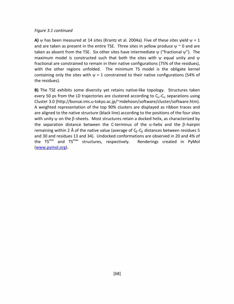
[68]
Figure 3.1 continued
A) ψ has been measured at 14 sites (Krantz et al. 2004a). Five of these sites yield ψ = 1 and are taken as present in the entire TSE. Three sites in yellow produce ψ ~ 0 and are taken as absent from the TSE. Six other sites have intermediate ψ (“fractional ψ”). The maximum model is constructed such that both the sites with ψ equal unity and ψ fractional are constrained to remain in their native configurations (75% of the residues), with the other regions unfolded. The minimum TS model is the obligate kernel containing only the sites with ψ = 1 constrained to their native configurations (54% of the residues).
B) The TSE exhibits some diversity yet retains native-like topology. Structures taken every 50 ps from the LD trajectories are clustered according to Cα-Cα separations using Cluster 3.0 (http://bonsai.ims.u-tokyo.ac.jp/~mdehoon/software/cluster/software.htm). A weighted representation of the top 90% clusters are displayed as ribbon traces and are aligned to the native structure (black line) according to the positions of the four sites with unity ψ on the β-sheets. Most structures retain a docked helix, as characterized by the separation distance between the C-terminus of the α-helix and the β-hairpin remaining within 2 Å of the native value (average of Cβ-Cβ distances between residues 5 and 30 and residues 13 and 34). Undocked conformations are observed in 20 and 4% of the TSmin and TSmax structures, respectively. Renderings created in PyMol (www.pymol.org).

[69]
1 identify the regions that are modeled in both initial TS models as unfolded or are left in their
native geometry, respectively. The TSmax model also initially constrains the fractional sites to
their native geometry, while these sites are permitted to become disrupted in the initial TSmin
model. The TS kernel is represented by TSmin and contains a four-stranded sheet network
docked against the carboxyl-terminal portion of the α-helix. The initial structures for the LD
simulations are generated by selectively disrupting those regions of the protein that are
assigned as unfolded in such a way that the global fold is undisturbed and the unfolded regions
retain physically plausible backbone dihedral angles. LD simulations use the implicit solvent
model developed in the Freed group (Shen and Freed 2001; 2002a) and implemented in a
modified version (Shen and Freed 2005) of the TINKER dynamics package (Ponder 1999). To
minimize the potential biases of different force fields, both the Garcia and Sanbonmatsu’s
modified Amber94 (G-S Amber94)(Garcia and Sanbonmatsu 2002) and the OPLS/AA-L (Kaminski
et al. 2000; 2001) force fields are utilized in separate simulations. Prior to any dynamics, the
energy of the initial structures is minimized with the added constraint that backbone torsional
angles of portions with native secondary structure remain close to their initial values. This
constraint is accomplished using a harmonic force constant of 1 kcal·mol-1·deg-2. Ten to twenty
10-40ns LD trajectories are performed for each TS model as well as for the native state. The
native sequence (i.e., without the biHis substitutions) is used in all simulations because the
experimental ψ-values are extrapolated to zero metal concentration and are corrected for the
change in stability due solely to the biHis substitution.
[70]
We introduce inter-residue distance constraints only at the five sites with ψ = 1 for
simulations of the transition and native states. The native Cβ-Cβ and Cα-Cα separations for these
five residue pairs are obtained from the crystal structure, and a relatively soft harmonic spring
(k = 2.4 kcal·mol-1∙Å-2) is used to maintain the crystal structure distances for these residue pairs
in the initial energy minimizations and in the LD simulations. In unrestrained TS simulations,
nearly all sites with ψ = 1 become displaced by at least 2 Å from their crystal structure positions
even though the structure remains relatively compact (the exception is site b which is located
near the turn of the β1-β2 hairpin). Distortions in these sites are partially due to the force field,
etc., because they also appear – but to a much lesser extent – in unrestrained native state
simulations, even though the average RMSD of the native state simulations is within 2 Å of the
crystal structure (data not shown). While the harmonic restraints are designed to maintain
native-like distances for these sites, we do not observe the TS models folding to the native
state. Reaching the native state requires the folding of both the 310 helix and β5 strand. These
barrier-crossing events are estimated to take 1-10µs, a timescale far beyond the LD
calculations.
Distributions of the inter-residue Cα-Cα and Cβ-Cβ distances are calculated for each
residue pair comprising a biHis site, first for individual trajectories and then averaged over all
trajectories. Both force fields yield similar results, so only data related to the OPLS/AA-L force
field are presented. The individual trajectories display a variety of behaviors, and comparing
the TSmin and TSmax models helps overcome any sampling issues and provides an indication of
the magnitude of structural diversity at the positions where ψ are fractional.
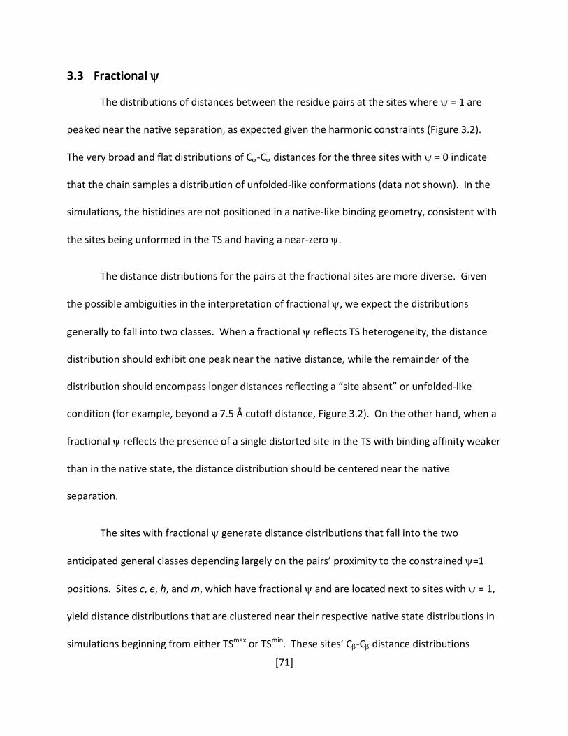
[71]
3.3 Fractional ψ
The distributions of distances between the residue pairs at the sites where ψ = 1 are
peaked near the native separation, as expected given the harmonic constraints (Figure 3.2).
The very broad and flat distributions of Cα-Cα distances for the three sites with ψ = 0 indicate
that the chain samples a distribution of unfolded-like conformations (data not shown). In the
simulations, the histidines are not positioned in a native-like binding geometry, consistent with
the sites being unformed in the TS and having a near-zero ψ.
The distance distributions for the pairs at the fractional sites are more diverse. Given
the possible ambiguities in the interpretation of fractional ψ, we expect the distributions
generally to fall into two classes. When a fractional ψ reflects TS heterogeneity, the distance
distribution should exhibit one peak near the native distance, while the remainder of the
distribution should encompass longer distances reflecting a “site absent” or unfolded-like
condition (for example, beyond a 7.5 Å cutoff distance, Figure 3.2). On the other hand, when a
fractional ψ reflects the presence of a single distorted site in the TS with binding affinity weaker
than in the native state, the distance distribution should be centered near the native
separation.
The sites with fractional ψ generate distance distributions that fall into the two
anticipated general classes depending largely on the pairs’ proximity to the constrained ψ=1
positions. Sites c, e, h, and m, which have fractional ψ and are located next to sites with ψ = 1,
yield distance distributions that are clustered near their respective native state distributions in
simulations beginning from either TSmax or TSmin. These sites’ Cβ-Cβ distance distributions
[72]
5 10 15 20
0.5
1.0
1.5
2.0
ψsite lexp = 0.90 ± 0.14
5 10 15 20
0.51.01.52.02.5
l
5 10 15 20
0.5
1.0
1.5
2.0
ψsite kexp = 0.48 ± 0.04
5 10 15 20
0.51.01.52.02.5
k
5 10 15 20
0.5
1.0
1.5
2.0
ψsite bexp = 1.06 ± 0.01
5 10 15 20
0.51.01.52.02.5
b
5 10 15 20
0.5
1.0
1.5
2.0
ψsite cexp = 0.52 ± 0.03
5 10 15 20
0.51.01.52.02.5
c
5 10 15 20
0.5
1.0
1.5
2.0
ψsite eexp = 0.75 ± 0.05
5 10 15 20
0.51.01.52.02.5
e
5 10 15 20
0.5
1.0
1.5
2.0
ψsite hexp = 0.57 ± 0.07
5 10 15 20
0.51.01.52.02.5
h
5 10 15 20
0.5
1.0
1.5
2.0
ψsite mexp = 0.26 ± 0.57
5 10 15 20
0.51.01.52.02.5
m
5 10 15 20
0.5
1.0
1.5
2.0
ψsite nexp = 0.53 ± 0.06
5 10 15 20
0.51.01.52.02.5
n
Unity
Distorted
Heterogeneous
Distance (Å)
C β-C
βD
istr
ibut
ion
C β-C
βD
istr
ibut
ion
C β-C
βD
istr
ibut
ion
Figure 3.2: Distributions of Cβ-Cβ Separations for N, TSmax, and TSmin States
(legend on next page)
[73]
Figure 3.2 continued
After an initial 2 ns equilibration period, distributions for the Cβ-Cβ separations in the Native (black), TSmax (red), and TSmin (red) simulations are calculated during the next 8 ns for 10-20 trajectories per model using the OPLS/AA-L force field. Inset: Cα-Cα distributions. The distributions for sites with ψ = 1 are centered near their native state separations from the crystal structure (solid black line) due to the imposed harmonic constraints. Some of the distributions at the sites with ψ = 1, e.g. site l, broaden due to departures from the native structure (see Figure 3.1). Fractional sites that represent distorted geometries (sites c, e, h, and m) have native-like Cα-Cα and Cβ-Cβ distributions with centroids below 7.5 Å (dashed line). Sites n and k exhibit distributions that sample both native-like and unfolded-like distributions for both the Cα-Cα and Cβ-Cβ distances.
[74]
exhibit some fine structure, but most of the distribution is below the 7.5Å cutoff, and their Cα-
Cα distributions are peaked near the native value. Evidently, the possible separations between
residue pairs at these fractional positions are hindered during the simulations by the
constraints imposed at the adjacent positions with ψ = 1.
Sites n and k are located further from the TS kernel and thus display broader
distributions in both their Cα-Cα and Cβ-Cβ distributions. Site n is situated at the distal end of
the amino-terminal hairpin, and site k is located on amino-terminal region of the α-helix. During
the LD trajectories, the separation between these two sites is indicative of whether a contact
between these two sites is present or not. Site n is formed initially in TSmax, and the distribution
of separation distances during the dynamics slightly exceeds the native distance (Figure 3.2).
Site n is absent in the beginning TSmin structure, and the resulting distance distributions are very
broad with minimal probability at the peak observed in simulations with TSmax. These two
results suggest the presence of two stable wells: one native-like and the other unfolded-like.
Site k appears as helical in the starting TSmax structure but as unfolded in TSmin and is the only
fractional site whose distribution of separations in the TSmax trajectories clearly suggests a
shuttling of this site between native-like and unfolded-like conformations (Figure 3.2). The site
k distributions for TSmax and TSmin are broad and extend from native-like to unfolded distances,
with TSmax favoring the former and TSmin the latter. The breadth of the distributions at larger
distances is consistent with an unfolded-like ensemble rather than a single conformation.
Figure 3.3 displays examples of the diverse behaviors observed in individual trajectories for
sites n and k. Compared to the other four sites with fractional ψ, sites k and n, the two sites

[75]
least affected by the constraints imposed on the five sites with ψ = 1, undergo fluctuations that
are best interpreted as TS heterogeneity.
This interpretation is further supported by an evaluation of the average number of
native hydrogen bonds formed (Figure 3.4A). The Cβ-Cβ separation at a site is an indicator of
whether a hydrogen bond is formed between the two residues. Typically, a native-like
separation implies hydrogen bond formation, while deviations from a native-like distance
implicate the loss of the corresponding hydrogen bond (Figure 3.3). Although fluctuations
between native-like and unfolded-like separations appear in trajectories for the distorted sites c
and e, the fluctuations are only observed in trajectories where the site is initially absent. The
separations in sites k and n fluctuate in more trajectories and in simulations for both TSmax and
TSmin.
This assessment presumes that the geometry of a distorted site remains hydrogen
bonded, while non-native separations imply the lack of hydrogen bonds. The fractional sites
located across two β-strands are associated with 1-2 hydrogen bonds. If at least one of these
hydrogen bonds is often formed and native-like, we believe that the fractional ψ of this site is
largely due to site distortion. Although the two different force fields differ quantitatively, the
overall trends are the same. A site with a fractional ψ situated near a site with ψ = 1 is more
likely to remain hydrogen bonded rather than fluctuate between native-like and unfolded-like
states. Overall, the simulations indicate that a fractional ψ may arise from either a distorted
site geometry, fluctuations between configurations with the hydrogen bond present and
absent, or some combination thereof.
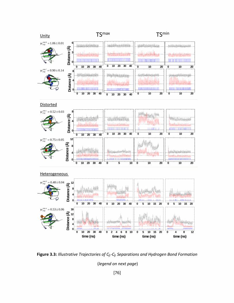
[76]
TSmax TSmin
b
l
k
c
e
n
0 10 20 30 400
3
6
Dist
ance
(Å)
0 10 20 30 40
0 10 20
0 10 20
0 10 20 30 400
4
8
Dist
ance
(Å)
0 10 20 30 40
0 10 20
0 10 20
0 10 20 30 400
4
8
Dist
ance
(Å)
0 10 20 30 40
0 10 20
0 10 20
0 10 20 30 40
0
4
8
12
Dist
ance
(Å)
0 5 10
0 10 20
0 10 20
0 10 20 30 400
4
8
12
Dist
ance
(Å)
0 10 20 30 40
0 5 10 15 20
0 5 10 15 20
0 10 20 30 400
4
8
12
16
Dist
ance
(Å)
time (ns)
0 2 4 6 8 10
time (ns)0 5 10 15 20
time (ns)0 4 8 12
time (ns)
01.006.1 siteexp ±=bψ
14.090.0 siteexp ±=lψ
03.052.0 siteexp ±=cψ
05.075.0 siteexp ±=eψ
06.053.0 siteexp ±=nψ
04.048.0 siteexp ±=kψ
Unity
Distorted
Heterogeneous
Figure 3.3: Illustrative Trajectories of Cβ-Cβ Separations and Hydrogen Bond Formation
(legend on next page)
[77]
Figure 3.3 continued
The Cβ-Cβ separation (black curve, distance in crystal structure denoted with dotted line) is presented along with the H-O distance for the hydrogen bond that is most associated with the Cβ-Cβ separation (red curve, 2.5 Å threshold separation is designated by black dotted line). The blue curve indicates whether the hydrogen bond is formed (1) or not formed (0). The Cβ-Cβ separation of sites with ψ = 1 remains close to their distance in the crystal structure. Sites with fractional ψ that emerge due to site distortion, e.g. sites c and e, experience some long-time fluctuations in which hydrogen bonds break and reform. These fluctuations occur primarily for trajectories where the sites begin in non-native conformations (TSmin). The two sites (k and n), whose behavior is indicative of structural heterogeneity, exhibit the most long-time fluctuations. A hydrogen bond is considered formed if the H-O distance is less than or equal to 2.5Å and the N-H-O angle is greater than 120°

[78]
a05
a13
b07
b13
d06
d67
g44
g70
l32 --
c06
c69
e04
e67
h42
h70
k28
m44
m68 n03
n17
0.00.20.40.60.81.01.2
N TSmax TSmin
fract
ion
hydr
ogen
bon
d
A)
B)
I3 L15 I30 L43 L67
<∆SASAU-TS>/<∆SASAU-N>
I3 L15 I30 L43 L670.0
0.5
1.0
<NNat-SC>/<NN,simNat-SC>
0.0
0.5
1.0 N,sim TSmax
TSmin
<NNat-SC>/NN,PDBNat-SC
<NTot-SC>/<NN,simTot-SC>
φ
Figure 3.4: Hydrogen Bond Formation and Computed φ
A) The average native hydrogen bond fraction is computed for the donor amide residue listed for the sites with unity and fractional ψ for Native (black), TSmax (red), and TSmin (blue) simulations. The average h-bond fraction for sites n and k (n03, n17, and k28) in the TS simulations tend to be less than the fractions for the other fractional sites. B) Average φ-values are computed using either total or native side chain contacts and computed relative to either the static PDB structure or the average of the native simulations. A contact is defined by two side chain heavy atoms within 5.5Å of one another and the corresponding residues are at least two residues away from each other. The experimentally measured φ (Sosnick et al. 2004; Went and Jackson 2005) are

[79]
Figure 3.4 continued
depicted by short horizontal bars. An alternative calculation uses the average solvent accessible solvent area (SASA) of the whole residue relative to the average SASA in an unfolded state ensemble constructed from a statistical coil library (Jha et al. 2005a). The data presented are computed using the OPLS/AA-L force field.
[80]
Varnai et al. (Varnai et al. 2008) also performed constrained simulations of Ub’s TSE.
However, they conclude that the ψ values do not adequately constrain the structure of the TSE,
contrary to the results of our simulations. The source of the discrepancy between the
simulations largely lies in a different implementation of the constraint for sites where ψ equals
unity, rather than differences in force fields or degree of sampling. We constrain the biHis sites
with ψ = 1 (i.e. native-like binding affinity) to have a near native separation by using a harmonic
potential. On the other hand, Varnai et al. allow the energy associated with the separation
distance to be constant over a broad range that extends out to rather long non-native
separations. The largest difference emerging from the two implementations occurs at the
helical site l with unity ψ, which remains intact throughout our simulations but unfolds during
their trajectories. Critically, the authors’ conclusions that data for ψ alone are insufficient to
constrain the TS are based largely on the unfolding of the helix in their simulations. Because
experiments indicate that the helix should remain intact, we believe their implementation of
the constraints and, hence, their conclusions are faulty.
In more detail, Varnai et al. define each ψsim as a smoothed step function with a drop-off
at each site’s native separation distance plus 3 Å. For each of the sites with zero or unity ψexp,
(ψsim -ψexp)2 is minimized in the simulations. The 3 Å tolerance distance is derived from His-His
separations observed in ion binding site geometries for a variety of proteins in the PDB. The
added range, however, allows both native and unfolded-like separations on the helix, because
both separations yield a value of unity for ψsim. In contrast, we contend that a ψ of unity
implies a native-like separation. Ub’s 3-turn helix remains largely intact in our implementation,
[81]
whereas it unfolds in their simulations. As further indication of the deficiency of their
implementation which induces the unfolding of the helix and disruption of the core, their
calculated φ for residues in the core are lower than what has been recorded in experiments.
Rather than the inability of ψ to properly define Ub’s TS, this under-reporting arises from a
combination of their poor implementation of the constraints, implied by the data for ψ, and
potentially the difficulty of calculating φ from simulations, as discussed in the next section.
3.4 Predicting φ from the TSE
With the TS structure independently determined from the data for ψ, we are well
positioned to investigate the ability of simulations to accurately predict experimental φ-values.
We have calculated φ from the number of side-chain heavy atom contacts in three different
ways. The customary manner is to compare the average number of native contacts in a
simulated TSE relative to the number of (native) contacts in the original (static) PDB structure
(Varnai et al. 2008). Two appealing alternatives are to calculate φ from the number of contacts
observed in simulations of the native and transition states, either using the total or only the
native (PDB) contacts.
Burial levels and φ for both TSmin and TSmax have been evaluated from the simulations
for five hydrophobic residues whose experimental φ have been measured (Figure 3.4B)(Sosnick
et al. 2004; Went and Jackson 2005). Each residue is highly buried in the TSE (>75%). The three
methods for calculating φ produce similar values across the five sites although the level varies
between the three methods from 0.3 to 0.7. All three methods yield significant deviations from
[82]
experiment, in particular over-predicting L67Aexpφ which is observed experimentally to vanish.
Calculations of φ using the total number of native contacts observed in simulations both of the
native and transition state agree with φexp at I3, L15 and I30, but over-predict the value at L43.
The customary method of using the number of native contacts relative to those in the static
PDB structure leads to an underestimate of φ at the first three sites, while the third option of
using the total number of contacts observed in simulations of both the native and transition
states always produces an overestimation of φ.
Based on these results, we believe that calculations of φ based on the number of side
chain contacts should not always agree with the experimental data. The most glaring issue for
the example of Ub is the significant over-prediction of φexp = 0 for the L67A substitution. This
discrepancy is not necessarily an error in the simulation per se, but in the mode of calculating φ.
Unlike the simulated values for φ, the experimental φexp reflect changes in free energy. The
observed lack of an energetic perturbation in the TSE for L67A can emerge due to multiple
factors, including relaxation and energy minimization of the structure (Bulaj and Goldenberg
2001; Sosnick et al. 2004; Baxa et al. 2008) or a change in intrinsic secondary structure
propensities of the substitution. Conversely, a vanishing experimental φ should not be taken as
an absolute indication that a site is devoid of structure in the TSE.
3.5 Conclusion
We have simulated models of Ub’s TSE by constraining the separations between the five
residue pairs for which experiments determine ψ as equal to unity. The constrained LD
trajectories indicate that the TSE is composed of an obligate kernel consisting of portions of β1-
[83]
β4 and the carboxyl-terminus of the α-helix. The periphery of the kernel relaxes to an energy
minimum structure, while the tails of the β1-β2 hairpin and the amino-terminus of the α-helix
are frayed. An analysis of the distribution of inter-residue separations indicates that fractional
ψ can reflect either a distorted binding site with weakened ion binding affinity or a site that
fluctuates between the hydrogen bond being present and being absent, especially for the two
sites distal to the sites with unity ψ. Calculations of φ using side-chain contacts for residues in
the core of the simulated TS often differ from those observed experimentally. Generally, one
should not expect agreement between theory and experiment because the experimental values
by definition reflect free energies rather than contacts. This discrepancy should be considered
in other studies that compare simulations to experimental data, particularly when the
experimentally determined TSE appears to be small and polarized.

[84]
4 Computing the Entropic Cost in Folding the Backbone of a Protein
The material in this chapter is currently in preparation for publication. I would like to thank Dr.
Abhishek Jha for laying the groundwork for this project as well as his helpful input. I would also
like to thank Joe DeBartolo for his assistance in generating structures.
Abstract
We calculate the loss of protein backbone entropy upon folding accounting for
correlations with the motions of neighboring residues. The entropy is calculated from the
difference in the Ramachandran distribution of backbone (φ,ψ) dihedral angles of each residue
in the unfolded state and in folded state. A previously developed statistical coil model for the
unfolded state provides the probabilities of occupying the five Ramachandran basins for each
residue. The distribution within each Ramachandran basin is calculated using intra-basin
Langevin dynamics simulations to compensate for the sparseness of the coil library. The
Ramachandran distribution of the native state is generated using Langevin dynamics. To
correct for reduction in diversity due to correlations with neighboring residues, the entropy is
also calculated considering the four dimensional probability distribution for two consecutive
residues (φi,ψi,φi+1,ψi+1). After including these corrections from the neighbor dependence of
backbone entropies, the average change in conformational entropy for each residue upon
folding, T∆SBBU-N = 0.7±0.3 kcal·mol-1 at 298 K. Our value is generally smaller than previous

[85]
calculations by 0.5-1 kcal·mol-1 because our unfolded state has less diversity and the ~ 0.3
kcal·mol-1 correction for correlated motions. We further analyze the results according to
residue type and location in the protein.

[86]
4.1 Introduction
The loss of backbone and side-chain conformational entropy is the largest unfavorable
quantity in the over-all stability of a protein. As such, an accurate calculation of ∆Sconf is needed
for the proper calculation of ∆G. In principle, the backbone entropy should be one of the most
straightforward thermodynamic quantities to compute. The calculation requires a suitable
ensemble of unfolded and folded structures which includes the diversity associated with
different secondary structures, amino acid types and burial levels. In addition, neighboring
residues affect a residue’s conformation (Zaman et al. 2003; Jha et al. 2005b) so that the
entropy of the chain is not the sum of the individual entropies determined for each residue.
Many approaches have been employed in attempts to calculate the loss of backbone
conformational entropy, ∆SBB, but none take into account all of these effects (Stites and
Pranata 1995; D'Aquino et al. 1996; Yang and Kay 1996; Meirovitch 2007). Some previous
analyses do not directly compare the backbone entropy in the native and unfold states, SBBN
and SBBU, or rely on assumptions or approximations concerning the structure and dynamics of
the two states. These methods have yielded values that differ by more than 0.5 kcal·mol-1 per
residue (at T = 300 K), or 50 kcal·mol-1 for a 100 residue protein. As this uncertainty is much
larger than the net stability, it is important to be able to accurately determine ∆SBB.
We address these issues by calculating the conformational entropy from the (φ,ψ)
probability distributions for both the folded and unfolded states of mammalian ubiquitin (Ub)
while accounting for correlated motions of adjacent residues (Zaman et al. 2003; Jha et al.
2005b). Our unfolded state ensemble is constructed using a highly restricted coil library that
[87]
accounts for the effect of neighboring residues on the each residue’s (φ,ψ) Ramachandran
distribution (Figure 4.1A). The coil library excludes helices, strands, turns and any residue
adjacent to these three types of hydrogen bonded structure. The ensemble recapitulates
global (radius of gyration) and local (NMR residual dipolar couplings) properties of chemically
denatured states (Jha et al. 2005a). A subset of this unfolded state ensemble is subjected to
intra-basin Langevin dynamics (LD) simulations to enhance conformational diversity. In order
to avoid potential bias due to the choice of force field, the LD unfolded state trajectories are
restrained so that each residue remains in its initial basin (Jha et al. 2005a) (Figure 4.1B). The
native state ensemble is generated from unconstrained LD simulations starting from the crystal
structure.
The conformational entropy is evaluated from the diversity of the Ramachandran
distribution, corrected for correlations with flanking residues. We find T∆SBBU-N = 0.7± 0.3
kcal·mol-1 with the exception of prolines (0.1± 0.1 kcal·mol-1) and pre-prolines (0.5± 0.2
kcal·mol-1). Although the average entropy of the unfolded state ensemble for all non-glycine,
proline, or pre-proline residue types are similar, individual positions in the sequence can exhibit
considerable variation due to the influence of neighboring residues in the unfolded state and,
to a lesser extent, in the folded state.

[88]
φ
ψ
β
α
αL
PPII other
Residue Q62unrestrainedrestrained to initial basin
initial
B)
Remove H-bonded structure (helix, sheet, turn, ~10% remaining)
A)
φψ
Figure 4.1: Generating the Unfolded State Ensemble
A) An initial unfolded state ensemble is generated from the statistical coil library described by Jha et al. (Jha et al. 2005a). Briefly, the PDB is parsed into a (non homologous) set of structures, and then regular hydrogen bonded residues with secondary structures are removed (upper). The resulting coil library is comprised of irregular tripeptides that primarily reside in the extended Ramachandran basins (lower). Images are taken from Figure 1E of ref. (Jha et al. 2005b). B) LD simulations provide the population distributions for averaging over the dihedral angles in individual Ramachandran basins. The coil library adequately provides the distribution among the

[89]
Figure 4.1 continued
Ramachandran basins, and intra-basin dynamics preserve this distribution as witnessed by the agreement with the experimental RDC measurements (Figure 4.3). In the absence of intra-basin restraints, residues freely sample other Ramachandran basins as shown in the case of Q62.

[90]
4.2 Methods
Unfolded State Ensemble: An initial ensemble of 13000 unfolded state structures is generated
from a coil library of (φ,ψ) dihedral angles composed of irregular, non-hydrogen bonded
structure (Jha et al. 2005a). Dihedral angles are selected contingent on both the flanking
residues’ chemical identity and conformation. To avoid steric overlap, these angles are
“nudged” by minimizing a simple excluded volume potential. This unfolded ensemble provides
the proper statistics for the distributions of each residue among the five major Ramachandran
basins. Short (100ps) all-atom intra-basin Langevin dynamics (LD) trajectories (as described
below) are run at 298 K for a randomly chosen subset (3,067) of these structures to obtain
adequate intra-basin sampling for evaluation of the backbone conformational entropy,
resulting in ensembles containing 306,700 structures.
Native State Ensemble: Ten 10 ns LD trajectories are run at 298 K starting from the energy
minimized crystal structure (1UBQ)(Vijay-Kumar et al. 1987). Structures after 1 ns are saved
every 1ps providing a total of 90,000 structures.
Langevin Dynamics Calculations: All-atom dynamic calculations use the TINKER v3.9 package
(Ponder 1999) which has been modified to increase computational efficiency (Shen and Freed
2005). The simulations utilize an implicit solvent model (Shen and Freed 2001; 2002a) with a
non-linear distance-dependent dielectric constant for the calculation of electrostatic
interactions (Jha and Freed 2008). Solute-solvent interactions are described by the Ooi-
Scheraga solvent accessible surface area potentials (Ooi et al. 1987), while the atomic friction
coefficients are computed with the Pastor-Karplus scheme (Pastor and Karplus 1988).
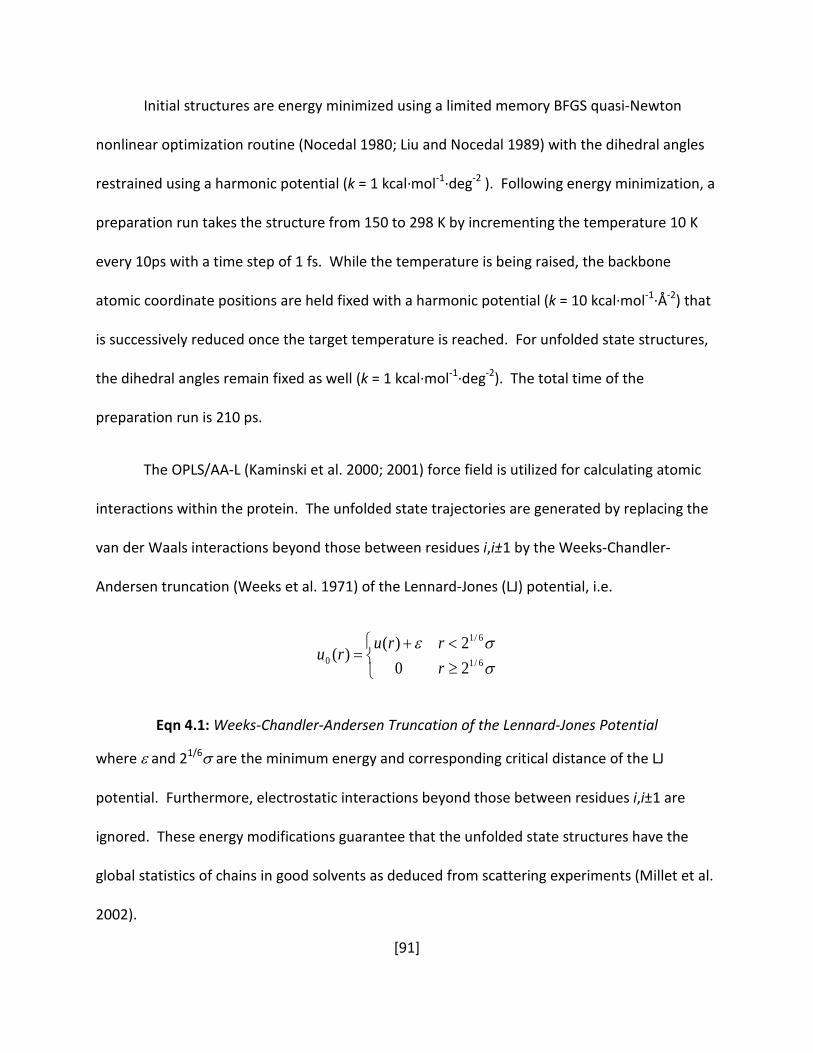
[91]
Initial structures are energy minimized using a limited memory BFGS quasi-Newton
nonlinear optimization routine (Nocedal 1980; Liu and Nocedal 1989) with the dihedral angles
restrained using a harmonic potential (k = 1 kcal·mol-1·deg-2 ). Following energy minimization, a
preparation run takes the structure from 150 to 298 K by incrementing the temperature 10 K
every 10ps with a time step of 1 fs. While the temperature is being raised, the backbone
atomic coordinate positions are held fixed with a harmonic potential (k = 10 kcal·mol-1∙Å-2) that
is successively reduced once the target temperature is reached. For unfolded state structures,
the dihedral angles remain fixed as well (k = 1 kcal·mol-1·deg-2). The total time of the
preparation run is 210 ps.
The OPLS/AA-L (Kaminski et al. 2000; 2001) force field is utilized for calculating atomic
interactions within the protein. The unfolded state trajectories are generated by replacing the
van der Waals interactions beyond those between residues i,i±1 by the Weeks-Chandler-
Andersen truncation (Weeks et al. 1971) of the Lennard-Jones (LJ) potential, i.e.
≥<+
=σσε
6/1
6/1
0 202)(
)(rrru
ru
Eqn 4.1: Weeks-Chandler-Andersen Truncation of the Lennard-Jones Potential where ε and 21/6σ are the minimum energy and corresponding critical distance of the LJ
potential. Furthermore, electrostatic interactions beyond those between residues i,i±1 are
ignored. These energy modifications guarantee that the unfolded state structures have the
global statistics of chains in good solvents as deduced from scattering experiments (Millet et al.
2002).
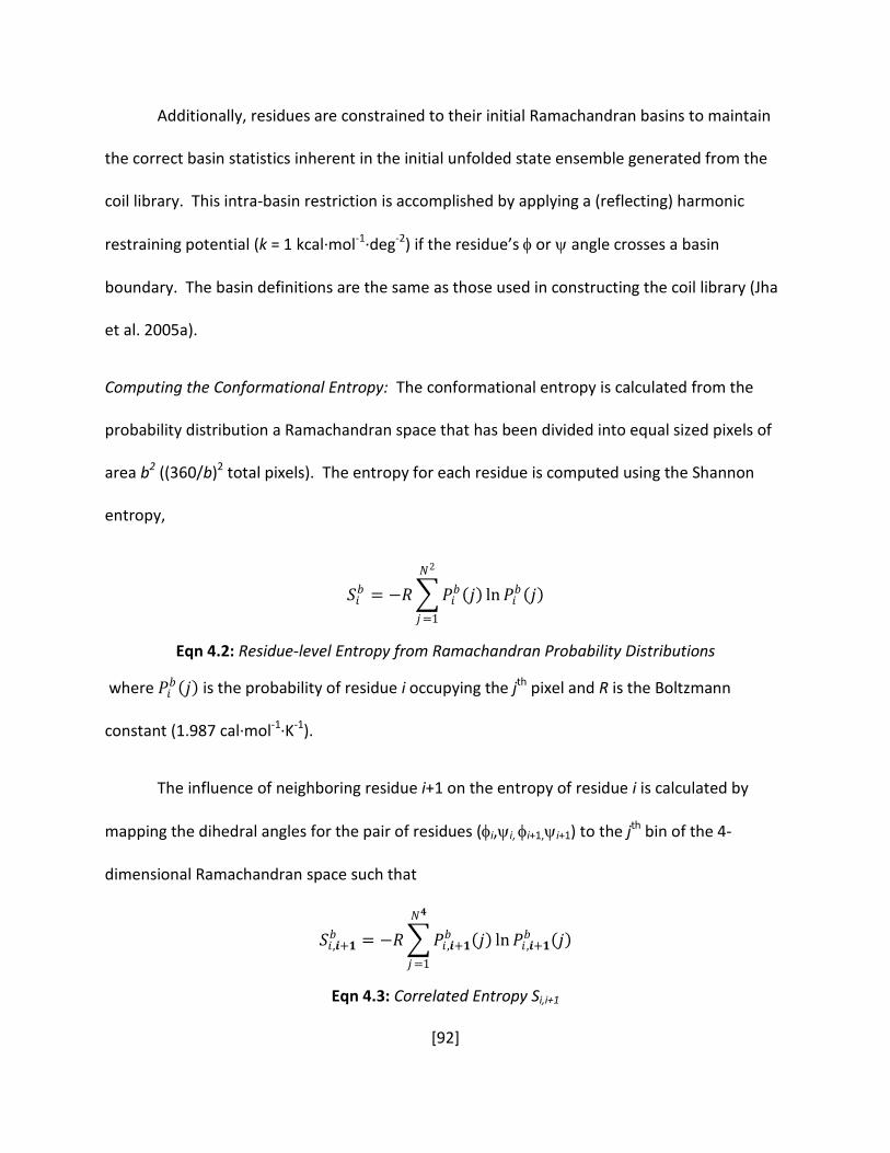
[92]
Additionally, residues are constrained to their initial Ramachandran basins to maintain
the correct basin statistics inherent in the initial unfolded state ensemble generated from the
coil library. This intra-basin restriction is accomplished by applying a (reflecting) harmonic
restraining potential (k = 1 kcal·mol-1·deg-2) if the residue’s φ or ψ angle crosses a basin
boundary. The basin definitions are the same as those used in constructing the coil library (Jha
et al. 2005a).
Computing the Conformational Entropy: The conformational entropy is calculated from the
probability distribution a Ramachandran space that has been divided into equal sized pixels of
area b2 ((360/b)2 total pixels). The entropy for each residue is computed using the Shannon
entropy,
𝑇𝑇𝑒𝑒𝑏𝑏 = −𝑅𝑅�𝑃𝑃𝑒𝑒𝑏𝑏(𝑗𝑗) ln𝑃𝑃𝑒𝑒𝑏𝑏(𝑗𝑗)𝑁𝑁2
𝑗𝑗=1
Eqn 4.2: Residue-level Entropy from Ramachandran Probability Distributions where 𝑃𝑃𝑒𝑒𝑏𝑏(𝑗𝑗) is the probability of residue i occupying the jth pixel and R is the Boltzmann
constant (1.987 cal·mol-1·K-1).
The influence of neighboring residue i+1 on the entropy of residue i is calculated by
mapping the dihedral angles for the pair of residues (φi,ψi, φi+1,ψi+1) to the jth bin of the 4-
dimensional Ramachandran space such that
𝑇𝑇𝑒𝑒 ,𝒊𝒊+𝟏𝟏𝑏𝑏 = −𝑅𝑅�𝑃𝑃𝑒𝑒 ,𝒊𝒊+𝟏𝟏𝑏𝑏 (𝑗𝑗) ln𝑃𝑃𝑒𝑒 ,𝒊𝒊+𝟏𝟏𝑏𝑏 (𝑗𝑗)𝑁𝑁𝟒𝟒
𝑗𝑗=1
Eqn 4.3: Correlated Entropy Si,i+1
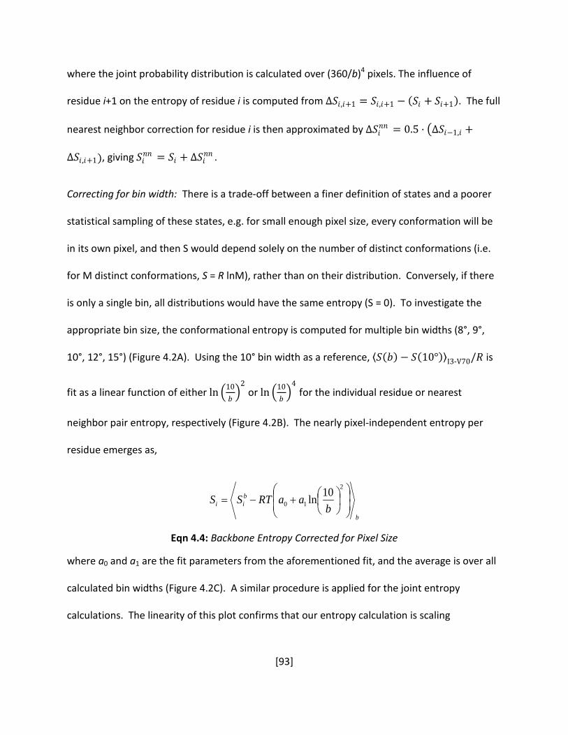
[93]
where the joint probability distribution is calculated over (360/b)4 pixels. The influence of
residue i+1 on the entropy of residue i is computed from Δ𝑇𝑇𝑒𝑒 ,𝑒𝑒+1 = 𝑇𝑇𝑒𝑒,𝑒𝑒+1 − (𝑇𝑇𝑒𝑒 + 𝑇𝑇𝑒𝑒+1). The full
nearest neighbor correction for residue i is then approximated by Δ𝑇𝑇𝑒𝑒𝑘𝑘𝑘𝑘 = 0.5 · �Δ𝑇𝑇𝑒𝑒−1,𝑒𝑒 +
Δ𝑇𝑇𝑒𝑒,𝑒𝑒+1), giving 𝑇𝑇𝑒𝑒𝑘𝑘𝑘𝑘 = 𝑇𝑇𝑒𝑒 + Δ𝑇𝑇𝑒𝑒𝑘𝑘𝑘𝑘 .
Correcting for bin width: There is a trade-off between a finer definition of states and a poorer
statistical sampling of these states, e.g. for small enough pixel size, every conformation will be
in its own pixel, and then S would depend solely on the number of distinct conformations (i.e.
for M distinct conformations, S = R lnM), rather than on their distribution. Conversely, if there
is only a single bin, all distributions would have the same entropy (S = 0). To investigate the
appropriate bin size, the conformational entropy is computed for multiple bin widths (8°, 9°,
10°, 12°, 15°) (Figure 4.2A). Using the 10° bin width as a reference, ⟨𝑇𝑇(𝑏𝑏) − 𝑇𝑇(10°)⟩I3-V70/𝑅𝑅 is
fit as a linear function of either ln �10𝑏𝑏�
2 or ln �10
𝑏𝑏�
4 for the individual residue or nearest
neighbor pair entropy, respectively (Figure 4.2B). The nearly pixel-independent entropy per
residue emerges as,
b
bii b
aaRTSS
+−=
2
1010ln
Eqn 4.4: Backbone Entropy Corrected for Pixel Size where a0 and a1 are the fit parameters from the aforementioned fit, and the average is over all
calculated bin widths (Figure 4.2C). A similar procedure is applied for the joint entropy
calculations. The linearity of this plot confirms that our entropy calculation is scaling

[94]
Figure 4.2: Correcting for Pixel Size in Entropy Calculations
A) The entropy values for the unfolded state ensemble are calculated for multiple pixel sizes. Entropy calculations for individual residue probability distributions P(φi,ψi) are shown with filled symbols, while the open symbols represent the entropy calculations over the joint probability distribution P(φi,ψi, φi+1,ψi+1) (See Methods). B) The 10°×10° pixel size is chosen as a reference point, and the average differences in entropies are fit
to a linear function of either ln �10𝑏𝑏�
2 or ln �10
𝑏𝑏�
4 for the individual or joint entropies,
respectively. C) The entropies calculated for different pixel sizes are corrected according
0 10 20 30 40 50 60 70 800
2
4
6
TS (k
cal·m
ol-1)
residue
8°×8° 10°×10° 15°×15° 9°×9° 12°×12°
-0.9 -0.6 -0.3 0.0 0.3 0.6-1.5
-1.0
-0.5
0.0
0.5
1.0
individual joint i,i +1
<S(b
)-S(1
0°)>
·R-1
ln(10°/b)n
0 10 20 30 40 50 60 70 800
2
4
6
TS (k
cal·m
ol-1)
residue
8°×8° 10°×10° 15°×15° 9°×9° 12°×12°
A)
B)
C)

[95]
Figure 4.2 continued
to the linear fit, which results in an entropy profile that independent of the choice in pixel size. The standard deviation from averaging over these corrected entropies are on the order of 0.1-0.2 kcal·mol-1.

[96]
appropriately with bin size b (ln(1/b)) and is not limited by the conformational diversity of our
ensembles or the coarseness of our bins.
4.3 Results and Discussion
4.3.1 Unfolded State Ensemble
The entropy of the unfolded ensemble created using a combination of PDB-based coil
library augmented using LD simulation is largely independent of position except for glycine,
proline and pre-proline residues. Because the conformational diversity of each residue is
affected by the neighboring residues, our entropy calculation for each residue includes the
influence of its two specific neighbors (e.g. V-R-K). Hence, the entropy calculation for Ub is
slightly different than our previous calculation for the same residue type in the coil library
where all neighbor combinations are allowed (e.g. V-R-K vs. X-R-Z, where X, Z are any residues)
(Jha et al. 2005b). The higher fidelity of the present calculation reduces the number of angles
at a given position. Hence, the distributions within each basin are averaged using LD
simulations but using constraints so that each residues remains within their original
Ramachandran basin. This calculation assumes that the total probability distribution may be
divided into two components: the inter-basin distribution (established by the propensities in
the coil library) and intra-basin fluctuations (obtained with all-atom LD simulations) (Perico et
al. 1993).
In order to maintain the basin assignments, which are likely to be biased by the force
field used in the LD simulation, each residue was restricted to its original basin determined
from the coil library using a harmonic reflecting “wall” at the edge of the basin (see Methods).
[97]
This procedure is especially necessary for computing nearest-neighbor effects, because of the
4-dimensional nature of the calculation.
To ensure that the LD generated ensemble still adequately models the local behavior
characteristic of the unfolded state, we compute the average residual dipolar coupling (RDC) for
each residue in Ub using a previously described protocol (Jha et al. 2005a) (Figure 4.3). The RDC
pattern derived from the LD simulations maintains good agreement with experimental data,
although the correlation coefficient is slightly reduced (R = 0.6, compared to 0.7). Nevertheless,
the similarity supports our protocol for generating diverse, LD-enhanced unfolded ensembles
while maintaining the physical characteristics of the initial ensemble.
4.3.2 The Change in Configuration Entropy in Folding
The loss of backbone entropy is calculated from the backbone entropy values of the
unfolded and native state ensembles (Figure 4.4). The largest change between states is found
along the β1-β2 hairpin and α-helix. Helical regions on average show a slightly larger loss in
backbone entropy compared to sheets and loop regions (0.86±0.18 versus 0.67±0.18 and
0.69±0.29 kcal·mol-1, respectively) (Figure 4.5, Table 4.1). Glycine residues exhibit an even
slightly larger loss in entropy (-T∆SBBU-N = 0.94±0.08 kcal·mol-1) than helical residues. Proline
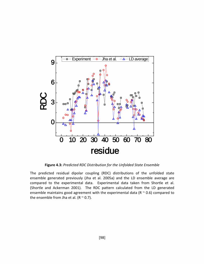
[98]
Figure 4.3: Predicted RDC Distribution for the Unfolded State Ensemble The predicted residual dipolar coupling (RDC) distributions of the unfolded state ensemble generated previously (Jha et al. 2005a) and the LD ensemble average are compared to the experimental data. Experimental data taken from Shortle et al. (Shortle and Ackerman 2001). The RDC pattern calculated from the LD generated ensemble maintains good agreement with the experimental data (R ~ 0.6) compared to the ensemble from Jha et al. (R ~ 0.7).
0 10 20 30 40 50 60 70 80
0
3
6
9
Experiment Jha et al. LD average
RDC
residue
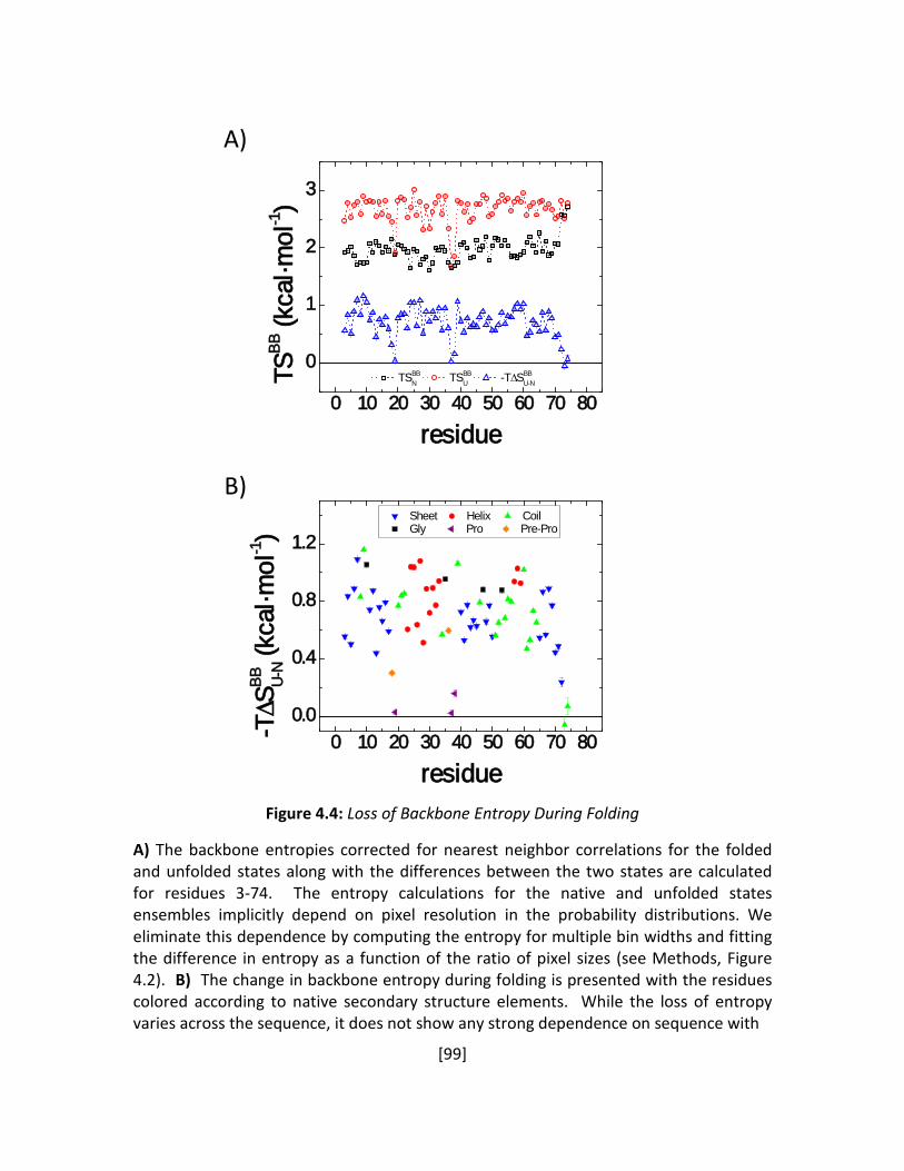
[99]
Figure 4.4: Loss of Backbone Entropy During Folding
A) The backbone entropies corrected for nearest neighbor correlations for the folded and unfolded states along with the differences between the two states are calculated for residues 3-74. The entropy calculations for the native and unfolded states ensembles implicitly depend on pixel resolution in the probability distributions. We eliminate this dependence by computing the entropy for multiple bin widths and fitting the difference in entropy as a function of the ratio of pixel sizes (see Methods, Figure 4.2). B) The change in backbone entropy during folding is presented with the residues colored according to native secondary structure elements. While the loss of entropy varies across the sequence, it does not show any strong dependence on sequence with
0 10 20 30 40 50 60 70 80
0
1
2
3
TSBBN TSBB
U -T∆SBBU-NTS
BB (k
cal·m
ol-1)
residue
0 10 20 30 40 50 60 70 800.0
0.4
0.8
1.2
Sheet Helix Coil Gly Pro Pre-Pro
-T∆S
BB U-N (
kcal
·mol
-1)
residue
A)
B)

[100]
Figure 4.4 continued
the exception of C-terminal, proline, and pre-proline residues. All of these residues have smaller changes in entropy during folding.
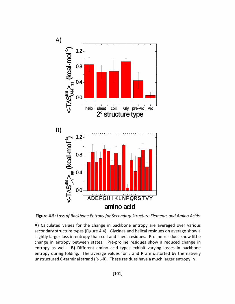
[101]
Figure 4.5: Loss of Backbone Entropy for Secondary Structure Elements and Amino Acids A) Calculated values for the change in backbone entropy are averaged over various secondary structure types (Figure 4.4). Glycines and helical residues on average show a slightly larger loss in entropy than coil and sheet residues. Proline residues show little change in entropy between states. Pre-proline residues show a reduced change in entropy as well. B) Different amino acid types exhibit varying losses in backbone entropy during folding. The average values for L and R are distorted by the natively unstructured C-terminal strand (R-L-R). These residues have a much larger entropy in
A)
B)
helix sheet coil Gly pre-Pro Pro
0.0
0.4
0.8
1.2
<-T∆
SBB
U-N
> ss (k
cal·m
ol-1)
2° structure type
ADEFGH I K L NPQRSTVY0.0
0.4
0.8
1.2
<-T∆
SBB
U-N
> aa (k
cal·m
ol-1)
amino acid

[102]
Figure 4.5 continued
the native state relative to other residues and, hence, a much smaller change in entropy (-0.06 – 0.24 kcal·mol-1).

[103]
Table 4.1: Average Loss of Backbone Entropy, T∆S, in Foldinga,b
Secondary Structure Type
<Global>
0.70 ± 0.26 Helix Sheet Loop Glycinec Pre-Proline Proline
0.86 ± 0.18 0.67 ± 0.18 0.69 ± 0.29 0.94 ± 0.08 0.45 ± 0.21 0.07 ± 0.08
Am
ino
Aci
d
A 0.65 ± 0.20 0.51 ± 0.01 -- 0.79 ± 0.02 -- -- -- D 0.87 ± 0.17 0.90 ± 0.18 -- 0.85 ± 0.21 -- -- -- E 0.65 ± 0.25 1.04 ± 0.02 0.79 ± 0.01 0.59 ± 0.05 -- 0.30 ± 0.01 -- F 0.74 ± 0.15 -- 0.73 ± 0.15 -- -- -- -- G 0.94 ± 0.08 -- -- -- 0.94 ± 0.08 -- -- H 0.89 ± 0.01 -- 0.89 ± 0.01 -- -- -- -- I 0.58 ± 0.10 0.66 ± 0.08 0.55 ± 0.12 0.47 ± 0.01 -- 0.60 ± 0.02 -- K 0.85 ± 0.15 0.97 ± 0.10 0.76 ± 0.12 0.73 ± 0.01 -- -- -- L 0.58 ± 0.27 -- 0.61 ± 0.10 0.82 ± 0.02d -- -- -- N 1.03 ± 0.01 1.04 ± 0.02 -- 1.02 ± 0.01 -- -- -- P 0.07 ± 0.08 -- -- -- -- -- 0.07 ± 0.08 Q 0.69 ± 0.16 0.89 ± 0.01 0.68 ± 0.13 0.53 ± 0.01 -- -- -- R 0.44 ± 0.34 -- 0.78 ± 0.01d 0.68 ± 0.02d -- -- -- S 0.75 ± 0.20 0.94 ± 0.01 0.55 ± 0.01 0.77 ± 0.02 -- -- -- T 0.92 ± 0.15 -- 0.90 ± 0.14 0.94 ± 0.19 -- -- -- V 0.54 ± 0.09 0.64 ± 0.01 0.51 ± 0.07 -- -- -- -- Y 0.93 ± 0.01 0.93 ± 0.01 -- -- -- -- --
a Units in kcal·mol-1 (T = 298K)
b Error values shown are the larger of either the standard deviation from averaging over multiple amino acids or propagated values from correcting for pixel sizes.
c Glycines for which we compute entropy changes are located along loop regions of Ub.
d These values exclude the unstructured C-terminal residues R72, L73, and R74, which have T∆S
= 0.24 ± 0.03, -0.06 ± 0.04, and 0.07 ± 0.06 kcal·mol-1, respectively. R72 is the terminal residue of β3 and exhibits an increase in backbone entropy in the native state ensemble due to fraying.

[104]
residues have similar backbone entropies in N and U (-T∆SBBU-N = 0.07±0.08 kcal·mol-1). Pre-
proline residues exhibit a lower change in backbone entropy between states (0.45±0.21
kcal·mol-1). Other differentiations similar to those described previously (Jha et al. 2005b) yield
little distinction between residues beyond proline, pre-proline, and all other residues.
Furthermore, the extent to which a residue is buried in the native state is weakly correlated
with the loss in backbone entropy (R ~ -0.2). Hence, the loss of backbone entropy is primarily
determined by local sequence effects rather than properties of the native state.
Our calculations of the entropy from probability distributions of (φ,ψ) angles is part of a
general class of Ramachandran-based calculations of the conformational entropy (Nemethy and
Scheraga 1965; Yang and Honig 1995; D'Aquino et al. 1996; Wang and Purisima 1996; Yang and
Kay 1996; Alexandrescu et al. 1998; Scott et al. 2007). The differences in our predictions and
others vary between 0.8-1.5 kcal·mol-1 due to restrictions in the probability distributions and
accounting for effects from flanking residues. The primary difference between these
approaches and ours has been in our use of a PDB-based statistical model of the unfolded state,
whereas the Ramachandran distributions used in the other studies are much broader. This
leads to an overestimation of 0.3-0.5 kcal·mol-1 in the loss of backbone entropy. Accordingly,
the predicted loss of entropy from these Ramachandran-based studies and others as well (Yang
and Honig 1995) are much larger than the values we predict (1.5-2.2 compared to 0.7±0.3
kcal·mol-1·residue-1).
The second difference between our results and others is our correction for correlated
motions. The conformational freedom of a residue not only depends on the amino acid type,

[105]
but also the chemical identity and conformation of its nearest neighbors (Figure 4.6). This
effect ranges between -0.2 and 0.5 kcal·mol-1 in our calculation of the loss in backbone entropy
and accounts for 0.1-0.3 kcal·mol-1 in the difference between the entropy of our unfolded state
and others. Dynamic simulations of dipeptides with a single (φ,ψ) angle between the two
planes (D'Aquino et al. 1996) would tend to overestimate the entropy of the unfolded state.
Another common method for measuring residue-level changes in entropy has been
through the Lipari-Szabo S2 order parameter (Lipari and Szabo 1982a; b) which probes
backbone NH bond vector motion on the pico- to nanosecond timescale. These methods have
resulted in changes in backbone entropy that range from 0.4 – 1.6 kcal·mol-1·residue-1 (Yang
and Kay 1996; Alexandrescu et al. 1998), which overlaps with the values we calculate. In
principle, the backbone motions probed by the NH bond vector motions are the same as the
dihedral motions we investigate. Hence, the differences in entropy should be the same as well
so long as individual NH vectors motions accurately report their associated peptide plane
motions in both the folded and unfolded states. Whether this assumption is true in the
unfolded state is unclear as there is no global reference frame. Furthermore, non-local and
other correlated chain motions could contribute to the measured S2 values even though these
motions do not contribute to backbone entropy.
The use of S2 values to calculate entropy requires applying a physical model to describe
the bond vector motion, typically one with azimuthal symmetry, such as free diffusion in a cone
(Yang and Kay 1996). However, the sampling of multiple Ramachandran basins indicates that a
model with azimuthal symmetry is invalid. As a result, a different relationship between entropy

[106]
Figure 4.6: Nearest Neighbor Corrections to the Backbone Entropy Corrections to the backbone entropy due to conformational correlations between nearest neighbors are displayed for both the folded and unfolded states. The corrections are larger in magnitude in the native state ensemble than in the unfolded state ensemble (T∆Snn = -0.3±0.1 and -0.2±0.1 kcal·mol-1, respectively). The turn regions between the β1-β2 hairpin and α-helix and the β4-β5 hairpin show the largest corrections in the native state, but pronounced corrections occur along other regions of the protein as well. The largest corrections in the unfolded state are associated with glycine and pre-glycine residues (T∆Snn = -0.28±0.03 kcal·mol-1) compared to all other residues (T∆Snn = -0.15±0.05 kcal·mol-1).
0 10 20 30 40 50 60 70 80-0.8-0.6-0.4-0.20.00.20.40.6
Folded Unfolded U-NT∆S nn
(kca
l·mol
-1)
residue
[107]
and S2 is required, and even then, a different one for the folded and unfolded states. These
issues may partially explain why measured values for S2 are quite variable in the unfolded state,
which introduces a significant uncertainty in the calculated loss of entropy upon folding.
Another empirical method for modeling the backbone entropy uses data from pulling
experiments of polyprotein chains (Thompson et al. 2002). Between periods of domain
unfolding, the force reduces the entropy of the unfolded chain. Analysis of the force extension
measurements provides a measure of the work needed to stretch a chain, which is equated to
the loss of entropy upon folding. Experiments for the α/β proteins I27 and I28 indicate that the
average entropy change for each residue associated with pulling is 1.4 ± 0.1 kcal·mol-1. This
calculation implicitly accounts for correlated motions and neighbor effects as the calculation is
for the entropy of the entire chain. However, the calculation assumes that the entropy of a
fully extended chain and the native state are the same. The disparity between this and our
calculation suggests that the fully extended chain has ~ 4-fold less states than the native state,
implying that the work required to pull the unfolded state to a fully extended chain exceeds the
backbone entropy lost during the folding of the protein. This difference could be explained by
the stretched chain being localized to narrow basin(s) near the φ ~ -ψ ∼ 180° region of the
Ramachandran map.
4.3.3 Ala→Gly Mutations
Our results enable us to comment on Ala→Gly comparisons that have served as the
benchmark for entropy and helical propensity calculations. Alanines have a much higher
propensity to be in a helical conformation than glycine residues, ∆GhelixA→G = 0.7 – 1 kcal·mol-1
[108]
(Creamer and Rose 1994; D'Aquino et al. 1996). This generally has been attributed to the
increase in conformational entropy in the unfolded state for glycine relative to alanine. In the
native Ub, Ala-28 is in an α-helix, while Ala-46 is located in a turn region (Figure 4.7). The
glycines exhibit unfolded state entropies that are largely independent of nearest neighbors
(Figure 4.8), and so in the case of Ala-28, our results would predict that an Ala→Gly mutation
would result in ∆(T∆SBBU-N)A28→G = 0.4 ± 0.1 kcal·mol-1. This value is less than previous
calculations (Nemethy and Scheraga 1965; D'Aquino et al. 1996), but agrees well with others
(Scott et al. 2007). However, we have now accounted for nearest neighbor effects in this
calculation and have more physically realistic probability distributions. The value we estimate is
primarily due to the reduced conformational freedom of Ala-28 in the unfolded state. By
comparison, the conformational diversity of Ala-46 in the unfolded state is on the same order
of the glycines such that ∆(T∆SBBU-N)A46→G = 0.2±0.1 kcal·mol-1. The differences in the entropies
of Ala-28 versus Ala-46 underscore the strong conformational effects of nearest neighbors in
the unfolded state ensemble. Furthermore, the predicted change in backbone entropy for
A28G is less than the measured change in helical propensity, indicating that other factors
contribute to the decrease in helical propensity beyond an increase in conformational entropy,
e.g. solvation or enthalphic effects. In fact, Jha et al. have shown that the difference in helical
propensity between alanines and glycines may be accounted for by the free energy required to
move a glycine from its preferred basins to the helical basin (Jha et al. 2005b). This free energy
difference is equally apportioned to entropic and enthalpic stabilization assuming ∆GhelixA→G =
0.7 – 1 kcal·mol-1. A similar conclusion was obtained by Scott et al., although their
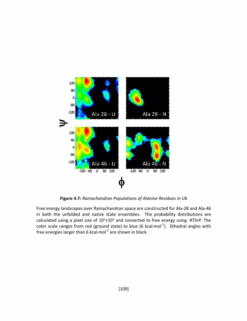
[109]
-120
-60
0
60
120
-120 -60 0 60 120
-120
-60
0
60
120
-120 -60 0 60 120
φ
ψ
Figure 4.7: Ramachandran Populations of Alanine Residues in Ub
Free energy landscapes over Ramachandran space are constructed for Ala-28 and Ala-46 in both the unfolded and native state ensembles. The probability distributions are calculated using a pixel size of 10°×10° and converted to free energy using -RTlnP. The color scale ranges from red (ground state) to blue (6 kcal·mol-1). Dihedral angles with free energies larger than 6 kcal·mol-1 are shown in black.

[110]
φ
ψ-120
-60
0
60
120
-120 -60 0 60 120
-120
-60
0
60
120
-120
-60
0
60
120
-120
-60
0
60
120
-120 -60 0 60 120
Unfolded Native
Figure 4.8: Ramachandran Populations of Glycine Residues in Ub
Unfolded and Native state free energy landscapes over Ramachandran space are shown for the glycine residues in Ub. The energy scale is the same as in Figure 4.7, with favored ground state set to 0 (shown in red) and states with energies larger than 6 kcal·mol-1 shown in black. Note that the glycines appear to have very similar distributions in the unfolded state ensembles.
[111]
Ramachandran distribution for Ala in the unfolded state is dominated by helical conformations
(Scott et al. 2007), whereas our distribution is dominated by extended conformations, as
necessary to recapitulate experimental RDC values.
4.4 Conclusions
We calculate the loss of backbone entropy upon folding using conformational
ensembles that account for the correlated motions between neighboring residues (Jha et al.
2005a). The ensembles also include realistic fine scale motions and sampling of Ramachandran
angles. Due to the correlated motions and the bias to extended conformers, as obtained from
the PDB-based coil library, our unfolded state ensemble is not as conformationally diverse as is
normally assumed. Upon folding, the number of available states is reduced by ~ 4-fold per
residue, except for prolines or pre-proline residues. Although our unfolded state ensemble has
less entropy than other models, this reduction does not resolve the Levinthal paradox because
the conformations often are not biased towards native structure. This situation is most
pronounced for helical proteins which have a high abundance of PPII and β conformers in the
unfolded state. As a result, the chain is biased to search through non-native states, a situation
which would only acerbate the search problem. However, the search problem can be resolved
by tertiary contacts stabilizing nascent native secondary structures elements.
[112]
5 Conclusions and Future Steps
5.1 Summary of Thesis Within the View of Protein Folding
General, predictive rules are largely absent in the study of protein folding mechanisms.
In my thesis, I have provided a basis for a seminal observation: the scaling of folding rate with
topological complexity. Three proteins with different topologies have been measured to have
TSEs adopting 60-80% of their respective native state topology. These results combined with
the observed correlation form the basis for our proposed 70% Rule of protein folding.
According to this rule, proteins fold through TSEs that adopt ~70% of the native state topology.
This high threshold places stringent limits on what structures could be part of the TSE.
The ψ-analysis method was utilized to generate residue-level models of the TSEs of
these proteins. In the case of Ub, we demonstrated that ψ could be used to generate a well
defined TSE. The ψ-generated TS models were used to evaluate the ability for simulations to
accurately predict experimental φ. A hydrophobic residue was found to be highly buried in the
TS, yet it results in a low to near-zero experimental φ. My simulations of Ub TSEs suggest that φ
probes the structural rigidity of the TS rather than specific structure formation.
Forming 70% of the native topology can be achieved with some non-native contacts.
Therefore, the TSE may energetically relax while still satisfying the 70% topology threshold.
This TS relaxation may lead to the underreporting of experimental φ (which reflects energies)
[113]
and, in the case of BdpA, experimental ψ. Both possibilities could result in an ill-defined TS or
the erroneous identification of a small and polarized TS.
Regardless of the possibility of TS relaxation, commensurate formation of secondary
structure and tertiary structure (e.g. hydrophobic burial) in the TS implies that regions of
regular structure are formed as well (Krantz et al. 2000; Krantz et al. 2002b). We believe that
hydrogen bonds and secondary structural elements (e.g. foldons) present in the TS form in a
step-wise manner prior to the TS since burying surface area promotes hydrogen bond
formation and vice versa. These results suggest then that proteins fold to a native-like topology
by successively forming units of structure in a sequential-like manner along the entire pathway.
In the last part of the thesis, I measured the loss of backbone entropy upon folding. I
created a PDB-based statistical coil model of the unfolded state ensemble using restrained
Langevin dynamics simulations while maintaining agreement with experimental determined
RDC values. The loss of backbone entropy during folding, T∆S = 0.7±0.3 kcal·mol-1 is less than
previous calculations by ~ 0.5-1 kcal·mol-1. This difference largely is a result of my unfolded
state ensemble being less structurally diverse and the correction for correlations between
adjacent residues. Although this reduction in unfolded state diversity appears to imply a
resolution of the Levinthal paradox, the remaining conformers are not generally biased towards
the native conformations. Therefore, rather than alleviating the conformational search in
folding, the unfolded state confounds the search problem by having the chain search through
unproductive conformations. This conundrum is resolved by tertiary contacts preferentially
stabilizing native-like regions of nascent secondary structure.
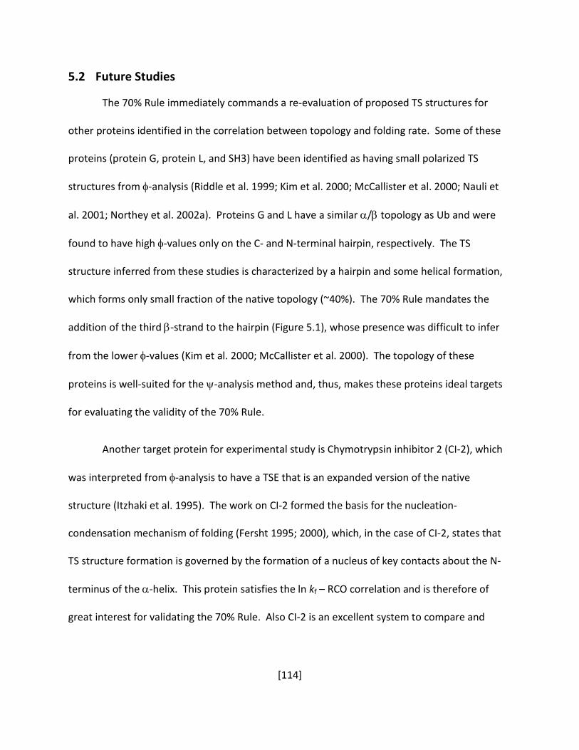
[114]
5.2 Future Studies
The 70% Rule immediately commands a re-evaluation of proposed TS structures for
other proteins identified in the correlation between topology and folding rate. Some of these
proteins (protein G, protein L, and SH3) have been identified as having small polarized TS
structures from φ-analysis (Riddle et al. 1999; Kim et al. 2000; McCallister et al. 2000; Nauli et
al. 2001; Northey et al. 2002a). Proteins G and L have a similar α/β topology as Ub and were
found to have high φ-values only on the C- and N-terminal hairpin, respectively. The TS
structure inferred from these studies is characterized by a hairpin and some helical formation,
which forms only small fraction of the native topology (~40%). The 70% Rule mandates the
addition of the third β-strand to the hairpin (Figure 5.1), whose presence was difficult to infer
from the lower φ-values (Kim et al. 2000; McCallister et al. 2000). The topology of these
proteins is well-suited for the ψ-analysis method and, thus, makes these proteins ideal targets
for evaluating the validity of the 70% Rule.
Another target protein for experimental study is Chymotrypsin inhibitor 2 (CI-2), which
was interpreted from φ-analysis to have a TSE that is an expanded version of the native
structure (Itzhaki et al. 1995). The work on CI-2 formed the basis for the nucleation-
condensation mechanism of folding (Fersht 1995; 2000), which, in the case of CI-2, states that
TS structure formation is governed by the formation of a nucleus of key contacts about the N-
terminus of the α-helix. This protein satisfies the ln kf – RCO correlation and is therefore of
great interest for validating the 70% Rule. Also CI-2 is an excellent system to compare and
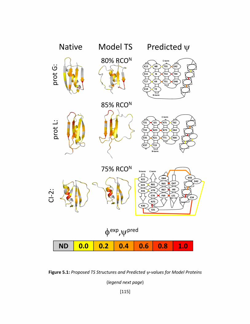
[115]
Q47
I49
L51E78
R81
V79
R65
R67
F69
D64K21
E23
P25
N-term C-term
K30
S31
N75
E34
K43D42
T2
K4
I6
N8
E19
T17
E15
K13
T51
T53
T55
D46
T44
E42
C-term
N-term
T19
K21
N23
I25
K37
E35
T33
T31
T71
N73
K75
A66
D64
T62
C-term
N-term
0.0 0.2 0.4 0.6 0.8ND 1.0
φexp,ψpred
prot
G:
Native
80% RCONpr
ot L
:
85% RCON
75% RCON
CI-2
:Model TS Predicted ψ
Figure 5.1: Proposed TS Structures and Predicted ψ-values for Model Proteins (legend next page)
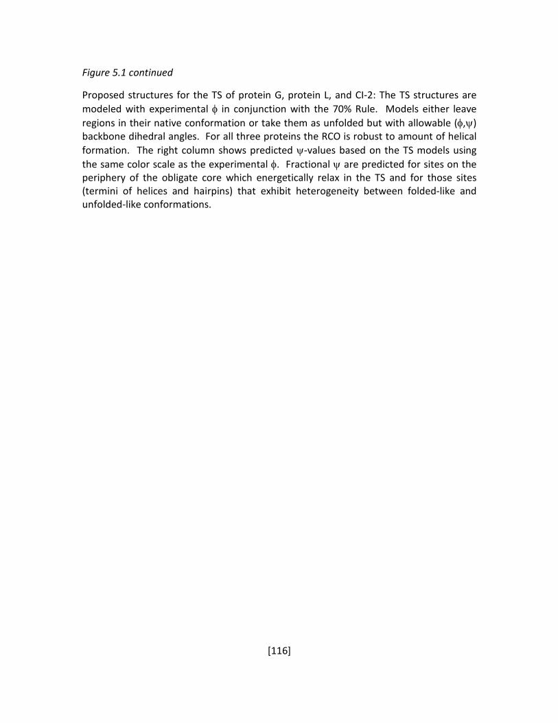
[116]
Figure 5.1 continued
Proposed structures for the TS of protein G, protein L, and CI-2: The TS structures are modeled with experimental φ in conjunction with the 70% Rule. Models either leave regions in their native conformation or take them as unfolded but with allowable (φ,ψ) backbone dihedral angles. For all three proteins the RCO is robust to amount of helical formation. The right column shows predicted ψ-values based on the TS models using the same color scale as the experimental φ. Fractional ψ are predicted for sites on the periphery of the obligate core which energetically relax in the TS and for those sites (termini of helices and hairpins) that exhibit heterogeneity between folded-like and unfolded-like conformations.
[117]
contrast the two major methods for characterizing TS structure. In Figure 5.1, we show
possible TS models that satisfy the 70% Rule, which can be tested experimentally using ψ-
analysis. If one observes unity ψ-values throughout the protein, as observed in Ub and Acp,
then CI-2’s TS is best described as native-like with partially unfolded regions, rather than an
“expanded version” of the native state (Itzhaki et al. 1995). Such a result would further
underscore the inherent uncertainties in the interpretation of φ-values.
5.3 Origins of the 70% Rule
A definite question deserving future study is to address the physical and biological
origins of the 70% Rule. It may be that this principle is an intrinsic property of cooperatively
folding proteins that bury (hydrophobic) surface area. In this case, it would be interesting to
understand what physical forces contribute to a threshold value of 70% rather than 50% or
90%.
Alternatively, the 70% Rule may be have a biological basis (Watters et al. 2007). A highly
native-like TS structure implies that there are few post-TS structures thermodynamically
accessible from the native state of the TS. Even if any such intermediates existed, they would
expose little additional surface area, which would reduce the chance for aggregation. If the
avoidance of aggregation underlies the 70% rule, aggregation prone regions should be
protected in a TS. This possibility could be examined using recently developed methods for
predicting aggregation prone regions (Tartaglia et al. 2008).

[118]
A more definitive testing of the origins of 70% Rule would be to characterize the TS of a
designed protein with no historical connection (homology) to a known protein, although it may
have a similar fold. The designed protein also should be a cooperative two-state folding protein
obeying the ln kf vs. RCO relationship. If the TS of the protein adopts 70% of the native state
topology, then the 70% Rule is likely an inherent property of cooperative proteins rather than a
result of evolutionary pressure to inhibit aggregation.
[119]
Appendix
ψ-analysis
ψ-analysis uses engineered biHis sites to probe the fraction of native metal ion binding
energy realized in the TS. The kinetic response as a function of metal ion concentration
quantifies the degree to which the biHis site is present in the TSE (see Refs.(Pandit et al. 2006;
Sosnick et al. 2006) for detailed treatment). In a manner analogous to the φ-analysis performed
using point mutations, the kinetic response due to metal binding can be obtained from the
denaturant dependence of folding rates (“chevron analysis”) at zero and high metal ion
concentrations.
When side chain substitution or metal binding only affects the unfolding rate ku and not
the free energy of the TS relative to the unfolded state, the structure probed is absent in the
TSE, and the corresponding φmutation or ψmetal vanishes. Conversely, when the perturbation only
affects the folding rate, kf, the structure probed is likely to be native-like in the TSE and the
associated φ- or a ψ-value is unity. When both the folding and unfolding arms shift, the φ- or ψ-
value is fractional, and the origin of a fractional value can be challenging to discern in both
methods. Fractional φ may arise either due to partial structure formation in the TS or to the
presence of multiple, distinct TS structures (Fersht et al. 1994; Kim et al. 1998; Martinez et al.
1998; Moran et al. 1999; Bulaj and Goldenberg 2001; Krantz and Sosnick 2001; Ozkan et al.
2001; Northey et al. 2002b). A fractional ψ-value indicates the biHis site is either native-like in a

[120]
subfraction of the TSE, or has non-native binding affinity in the entire TSE (e.g. a distorted site
with less favorable binding geometry, or a flexible site that must be restricted prior to ion
binding), or some combination thereof (Krantz et al. 2004a; Sosnick et al. 2004)(D. Goldenberg,
private communication).
ψ-analysis has the powerful capability of generating a large quantity of high quality
kinetic data to accurately probe the degree to which a particular binding site is formed in the
TSE. Each biHis variant enables the measurement of dozens of folding rates at increasing
concentrations of metal ions. The binding of increasing concentrations of ions to the biHis site
produces a nearly continuous increase in the stability of TS structures that contain the binding
site. Hence, the stability is perturbed yet accomplished in an isosteric and isochemical manner.
The resulting series of data can be justifiably combined, a process which may be inappropriate
in traditional mutation studies where the perturbation can arise from multiple sources,
including changes in backbone propensities as well as indeterminate non-local interactions.
The ψ-analysis data can be represented as a Leffler plot where the change in activation
free energy is plotted relative to the change in the metal-induced stability (Leffler 1953) (Figure
2.3C). If the biHis site is formed in the TSE, metal binding increases its stability, and folding
rates increase. The associated Leffler plot has a positive slope as both ΔΔ𝐺𝐺𝑓𝑓‡
and ΔΔ𝐺𝐺𝑒𝑒𝑒𝑒
increase.
The starting point in the detailed interpretation of the Leffler plot involves fitting the
data to a model with a single free parameter ψo, which is the slope at the origin in the absence
of metal,
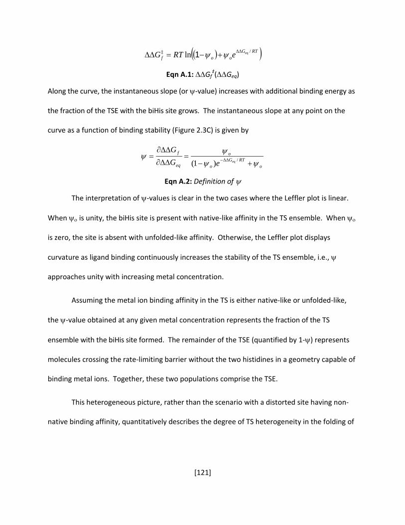
[121]
( )( )RTGoof
eqeRTG /‡ ln ∆∆+−=∆∆ ψψ1
Eqn A.1: ∆∆Gf‡(∆∆Geq)
Along the curve, the instantaneous slope (or ψ-value) increases with additional binding energy as
the fraction of the TSE with the biHis site grows. The instantaneous slope at any point on the
curve as a function of binding stability (Figure 2.3C) is given by
oRTG
o
o
eq
f
eqeGG
ψψψ
ψ+−
=∆∆∂
∆∆∂= ∆∆− /)1(
Eqn A.2: Definition of ψ
The interpretation of ψ-values is clear in the two cases where the Leffler plot is linear.
When ψο is unity, the biHis site is present with native-like affinity in the TS ensemble. When ψο
is zero, the site is absent with unfolded-like affinity. Otherwise, the Leffler plot displays
curvature as ligand binding continuously increases the stability of the TS ensemble, i.e., ψ
approaches unity with increasing metal concentration.
Assuming the metal ion binding affinity in the TS is either native-like or unfolded-like,
the ψ-value obtained at any given metal concentration represents the fraction of the TS
ensemble with the biHis site formed. The remainder of the TSE (quantified by 1-ψ) represents
molecules crossing the rate-limiting barrier without the two histidines in a geometry capable of
binding metal ions. Together, these two populations comprise the TSE.
This heterogeneous picture, rather than the scenario with a distorted site having non-
native binding affinity, quantitatively describes the degree of TS heterogeneity in the folding of
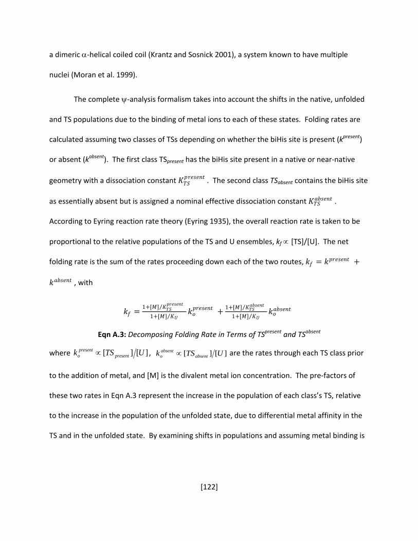
[122]
a dimeric α-helical coiled coil (Krantz and Sosnick 2001), a system known to have multiple
nuclei (Moran et al. 1999).
The complete ψ-analysis formalism takes into account the shifts in the native, unfolded
and TS populations due to the binding of metal ions to each of these states. Folding rates are
calculated assuming two classes of TSs depending on whether the biHis site is present (kpresent)
or absent (kabsent). The first class TSpresent has the biHis site present in a native or near-native
geometry with a dissociation constant 𝐾𝐾𝑇𝑇𝑇𝑇𝑝𝑝𝑟𝑟𝑒𝑒𝑟𝑟𝑒𝑒𝑘𝑘𝑟𝑟 . The second class TSabsent contains the biHis site
as essentially absent but is assigned a nominal effective dissociation constant 𝐾𝐾𝑇𝑇𝑇𝑇𝑎𝑎𝑏𝑏𝑟𝑟𝑒𝑒𝑘𝑘𝑟𝑟 .
According to Eyring reaction rate theory (Eyring 1935), the overall reaction rate is taken to be
proportional to the relative populations of the TS and U ensembles, kf ∝ [TS]/[U]. The net
folding rate is the sum of the rates proceeding down each of the two routes, 𝑘𝑘𝑓𝑓 = 𝑘𝑘𝑝𝑝𝑟𝑟𝑒𝑒𝑟𝑟𝑒𝑒𝑘𝑘𝑟𝑟 +
𝑘𝑘𝑎𝑎𝑏𝑏𝑟𝑟𝑒𝑒𝑘𝑘𝑟𝑟 , with
𝑘𝑘𝑓𝑓 = 1+[𝑀𝑀] 𝐾𝐾𝑇𝑇𝑇𝑇𝑝𝑝𝑟𝑟𝑒𝑒𝑟𝑟𝑒𝑒𝑘𝑘𝑟𝑟⁄
1+[𝑀𝑀] 𝐾𝐾𝑈𝑈⁄ 𝑘𝑘𝑜𝑜𝑝𝑝𝑟𝑟𝑒𝑒𝑟𝑟𝑒𝑒𝑘𝑘𝑟𝑟 + 1+[𝑀𝑀] 𝐾𝐾𝑇𝑇𝑇𝑇
𝑎𝑎𝑏𝑏𝑟𝑟𝑒𝑒𝑘𝑘𝑟𝑟⁄1+[𝑀𝑀] 𝐾𝐾𝑈𝑈⁄ 𝑘𝑘𝑜𝑜𝑎𝑎𝑏𝑏𝑟𝑟𝑒𝑒𝑘𝑘𝑟𝑟
Eqn A.3: Decomposing Folding Rate in Terms of TSpresent and TSabsent
where ][][ UTSk presentpresent
o ∝ , ][][ UTSk absentabsento ∝ are the rates through each TS class prior
to the addition of metal, and [M] is the divalent metal ion concentration. The pre-factors of
these two rates in Eqn A.3 represent the increase in the population of each class’s TS, relative
to the increase in the population of the unfolded state, due to differential metal affinity in the
TS and in the unfolded state. By examining shifts in populations and assuming metal binding is
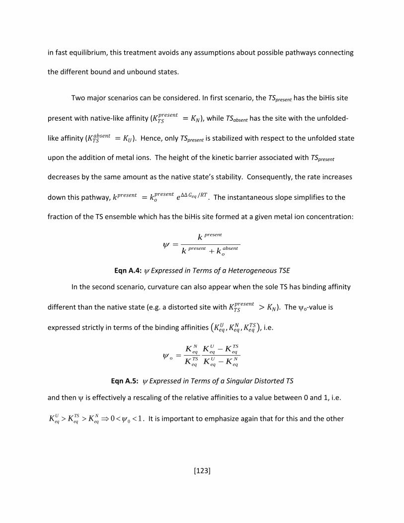
[123]
in fast equilibrium, this treatment avoids any assumptions about possible pathways connecting
the different bound and unbound states.
Two major scenarios can be considered. In first scenario, the TSpresent has the biHis site
present with native-like affinity (𝐾𝐾𝑇𝑇𝑇𝑇𝑝𝑝𝑟𝑟𝑒𝑒𝑟𝑟𝑒𝑒𝑘𝑘𝑟𝑟 = 𝐾𝐾𝑁𝑁), while TSabsent has the site with the unfolded-
like affinity (𝐾𝐾𝑇𝑇𝑇𝑇𝑎𝑎𝑏𝑏𝑟𝑟𝑒𝑒𝑘𝑘𝑟𝑟 = 𝐾𝐾𝑈𝑈). Hence, only TSpresent is stabilized with respect to the unfolded state
upon the addition of metal ions. The height of the kinetic barrier associated with TSpresent
decreases by the same amount as the native state’s stability. Consequently, the rate increases
down this pathway, 𝑘𝑘𝑝𝑝𝑟𝑟𝑒𝑒𝑟𝑟𝑒𝑒𝑘𝑘𝑟𝑟 = 𝑘𝑘𝑜𝑜𝑝𝑝𝑟𝑟𝑒𝑒𝑟𝑟𝑒𝑒𝑘𝑘𝑟𝑟 𝑒𝑒ΔΔ𝐺𝐺𝑒𝑒𝑒𝑒 /𝑅𝑅𝑇𝑇 . The instantaneous slope simplifies to the
fraction of the TS ensemble which has the biHis site formed at a given metal ion concentration:
absento
present
present
kk
k
+=ψ
Eqn A.4: ψ Expressed in Terms of a Heterogeneous TSE In the second scenario, curvature can also appear when the sole TS has binding affinity
different than the native state (e.g. a distorted site with 𝐾𝐾𝑇𝑇𝑇𝑇𝑝𝑝𝑟𝑟𝑒𝑒𝑟𝑟𝑒𝑒𝑘𝑘𝑟𝑟 > 𝐾𝐾𝑁𝑁). The ψo-value is
expressed strictly in terms of the binding affinities �𝐾𝐾𝑒𝑒𝑒𝑒𝑈𝑈 ,𝐾𝐾𝑒𝑒𝑒𝑒𝑁𝑁 ,𝐾𝐾𝑒𝑒𝑒𝑒𝑇𝑇𝑇𝑇�, i.e.
Neq
Ueq
TSeq
Ueq
TSeq
Neq
KKKK
KK
−
−=oψ
Eqn A.5: ψ Expressed in Terms of a Singular Distorted TS and then ψ is effectively a rescaling of the relative affinities to a value between 0 and 1, i.e.
10 0 <<⇒>> ψNeq
TSeq
Ueq KKK . It is important to emphasize again that for this and the other

[124]
scenarios, the ψ = 0 and 1 values still imply that the biHis site is absent or 100% present in the
TSE, respectively.
[125]
References
Abkevich, V.I., Gutin, A.M., and Shakhnovich, E.I. 1994. Specific nucleus as the transition state for protein folding: evidence from the lattice model. Biochemistry 33: 10026-10036.
Alexandrescu, A.T., Rathgeb-Szabo, K., Rumpel, K., Jahnke, W., Schulthess, T., and Kammerer, R.A. 1998. 15N backbone dynamics of the S-peptide from ribonuclease A in its free and S-protein bound forms: toward a site-specific analysis of entropy changes upon folding. Protein Sci 7: 389-402.
Alonso, D.O., and Daggett, V. 2000. Staphylococcal protein A: unfolding pathways, unfolded states, and differences between the B and E domains. Proc. Natl. Acad. Sci. U S A 97: 133-138.
Arora, P., Oas, T.G., and Myers, J.K. 2004. Fast and faster: a designed variant of the B-domain of protein A folds in 3 microsec. Protein Sci. 13: 847-853.
Astbury, W.T. 1933. Some problems in the X-ray analysis of the structure of animal hairs and other protein fibres. Transactions of the Faraday Society 29: 193-205.
Bai, Y., Karimi, A., Dyson, H.J., and Wright, P.E. 1997. Absence of a stable intermediate on the folding pathway of protein A. Protein Sci 6: 1449-1457.
Bai, Y., Sosnick, T.R., Mayne, L., and Englander, S.W. 1995. Protein folding intermediates: native-state hydrogen exchange. Science 269: 192-197.
Bai, Y., Zhou, H., and Zhou, Y. 2004. Critical nucleation size in the folding of small apparently two-state proteins. Protein Sci. 13: 1173-1181.
Balch, W.E., Morimoto, R.I., Dillin, A., and Kelly, J.W. 2008. Adapting proteostasis for disease intervention. Science 309: 916-919.
Baxa, M.C., Freed, K.F., and Sosnick, T.R. 2008. Quantifying the structural requirements of the folding transition state of protein A and other systems. J Mol Biol 381: 1362-1381.
Berman, H.M., Bhat, T.N., Bourne, P.E., Feng, Z., Gilliland, G., Weissig, H., and Westbrook, J. 2000. The Protein Data Bank and the challenge of structural genomics. Nat Struct Biol 7 Suppl: 957-959.
[126]
Bernado, P., Blanchard, L., Timmins, P., Marion, D., Ruigrok, R.W., and Blackledge, M. 2005. A structural model for unfolded proteins from residual dipolar couplings and small-angle x-ray scattering. Proc Natl Acad Sci U S A 102: 17002-17007.
Berriz, G.F., and Shakhnovich, E.I. 2001. Characterization of the folding kinetics of a three-helix bundle protein via a minimalist Langevin model. J. Mol. Biol. 310: 673-685.
Boczko, E.M., and Brooks, C.L., 3rd. 1995. First-principles calculation of the folding free energy of a three-helix bundle protein. Science 269: 393-396.
Bodenreider, C., and Kiefhaber, T. 2005. Interpretation of protein folding psi values. J Mol Biol 351: 393-401.
Bosco, G., Baxa, M., and Sosnick, T. 2009. Metal binding kinetics of bi-Histidine sites used in Psi-analysis: Evidence for high energy protein folding intermediates. Biochemistry.
Brandts, J.F. 1964. Thermodynamics of Protein Denaturation .2. Model of Reversible Denaturation + Interpretations Regarding Stability of Chymotrypsinogen. Journal of the American Chemical Society 86: 4302-&.
Bulaj, G., and Goldenberg, D.P. 2001. Phi-values for BPTI folding intermediates and implications for transition state analysis. Nature Struct. Biol. 8: 326-330.
Bullock, A., and Fersht, A. 2001. Rescuing the function of mutant p53. Nature Rev. Cancer 1: 68-76.
Capaldi, A.P., Kleanthous, C., and Radford, S.E. 2002. Im7 folding mechanism: misfolding on a path to the native state. Nature Struct. Biol.
Cheng, S., Yang, Y., Wang, W., and Liu, H. 2005. Transition state ensemble for the folding of B domain of protein A: a comparison of distributed molecular dynamics simulations with experiments. J Phys Chem B 109: 23645-23654.
Connelly, G.P., Bai, Y., Jeng, M.-F., Mayne, L., and Englander, S.W. 1993. Isotope effects in peptide group hydrogen exchange. Proteins 17: 87-92.
Creamer, T.P., and Rose, G.D. 1994. Alpha-helix-forming propensities in peptides and proteins. Proteins 19: 85-97.
D'Aquino, J.A., Gomez, J., Hilser, V.J., Lee, K.H., Amzel, L.M., and Freire, E. 1996. The magnitude of the backbone conformational entropy change in protein folding. Proteins 25: 143-156.
Daggett, V. 2001. Molecular dynamics simulations of protein unfolding/folding. Methods Mol. Biol. 168: 215-247.
[127]
Dill, K.A., and Chan, H.S. 1997. From Levinthal to pathways to funnels. Nature Struct. Biol. 4: 19.
Dill, K.A., Ozkan, S.B., Weikl, T.R., Chodera, J.D., and Voelz, V.A. 2007. The protein folding problem: when will it be solved? Curr Opin Struct Biol 17: 342-346.
Dimitriadis, G., Drysdale, A., Myers, J.K., Arora, P., Radford, S.E., Oas, T.G., and Smith, D.A. 2004. Microsecond folding dynamics of the F13W G29A mutant of the B domain of staphylococcal protein A by laser-induced temperature jump. Proc Natl Acad Sci U S A 101: 3809-3814.
Dyson, H., and Wright, P. 2005. Intrinsically unstructured proteins and their functions. Nature Rev. Mol. Cell Biol. 6: 197-208.
Dyson, H.J., and Wright, P.E. 2002. Coupling of folding and binding for unstructured proteins. Curr. Opin. Struct. Biol. 12: 54-60.
Englander, S.W., Sosnick, T.R., Mayne, L.C., Shtilerman, M., Qi, P.X., and Bai, Y. 1998. Fast and Slow Folding in Cytochrome C. Accts. of Chem. Res. 31: 737-744.
Eyring, H. 1935. The activated complex in chemical reactions. J. Chem. Phys. 3: 107-115.
Feng, H., Vu, N.D., Zhou, Z., and Bai, Y. 2004. Structural examination of Phi-value analysis in protein folding. Biochemistry 43: 14325-14331.
Fersht, A.R. 1995. Optimization of rates of protein folding: the nucleation-condensation mechanism and its implications. Proc. Natl. Acad. Sci. USA 92: 10869-10873.
Fersht, A.R. 2000. Transition-state structure as a unifying basis in protein-folding mechanisms: contact order, chain topology, stability, and the extended nucleus mechanism. Proc Natl Acad Sci U S A 97: 1525-1529.
Fersht, A.R. 2004. φ value versus ψ analysis. Proc. Natl. Acad. Sci. U S A. 101: 17327-17328.
Fersht, A.R., Itzhaki, L.S., elMasry, N.F., Matthews, J.M., and Otzen, D.E. 1994. Single versus parallel pathways of protein folding and fractional formation of structure in the transition state. Proc. Natl. Acad. Sci. USA 91: 10426-10429.
Fersht, A.R., Matouschek, A., and Serrano, L. 1992. The folding of an enzyme. I. Theory of protein engineering analysis of stability and pathway of protein folding. J. Mol. Biol. 224: 771-782.
Garbuzynskiy, S.O., Finkelstein, A.V., and Galzitskaya, O.V. 2005. On the Prediction of Folding Nuclei in Globular Proteins. Mol. Biology. 39: 906-914.

[128]
Garcia-Mira, M.M., Boehringer, D., and Schmid, F.X. 2004. The folding transition state of the cold shock protein is strongly polarized. J. Mol. Biol. 339: 555-569.
Garcia, A.E., and Onuchic, J.N. 2003. Folding a protein in a computer: An atomic description of the folding/unfolding of protein A. Proc Natl Acad Sci U S A 100: 13898-13903.
Garcia, A.E., and Sanbonmatsu, K.Y. 2002. alpha -Helical stabilization by side chain shielding of backbone hydrogen bonds. Proc. Natl. Acad. Sci. U S A 99: 2782-2787.
Ghosh, A., Elber, R., and Scheraga, H.A. 2002. An atomically detailed study of the folding pathways of protein A with the stochastic difference equation. Proc Natl Acad Sci U S A 99: 10394-10398.
Goldenberg, D.P. 1992. Mutational Analysis of Protein Folding and Stability. In Protein Folding. (ed. T.E. Creighton), pp. 353-403. W. H. Freeman, New York.
Goldenberg, D.P. 1999. Finding the right fold. Nature Struct. Biol. 6: 987-990.
Goldenberg, D.P., Frieden, R.W., Haack, J.A., and Morrison, T.B. 1989. Mutational analysis of a protein-folding pathway. Nature: 127-132.
Grantcharova, V.P., Riddle, D.S., Santiago, J.V., and Baker, D. 1998. Important role of hydrogen bonds in the structurally polarized transition state for folding of the src SH3 domain. Nature Struct. Biol. 5: 714-720.
Gruebele, M., and Wolynes, P.G. 1998. Satisfying turns in folding transitions. Nature Struct. Biol. 5: 662-665.
Guo, W., Lampoudi, S., and Shea, J.E. 2004. Temperature dependence of the free energy landscape of the src-SH3 protein domain. Proteins 55: 395-406.
Guo, Z., Brooks, C.L., 3rd, and Boczko, E.M. 1997. Exploring the folding free energy surface of a three-helix bundle protein. Proc. Natl. Acad. Sci. U S A 94: 10161-10166.
Guo, Z.Y., and Thirumalai, D. 1995. Kinetics of protein-folding: nucleation mechanism, time scales, and pathways. Biopolymers 36: 83-102.
Hua, Q.X., Ladbury, J.E., and Weiss, M.A. 1993. Dynamics of a monomeric insulin analogue: testing the molten-globule hypothesis. Biochemistry 32: 1433-1442.
Islam, S.A., Karplus, M., and Weaver, D.L. 2002. Application of the diffusion-collision model to the folding of three-helix bundle proteins. J. Mol. Biol. 318: 199-215.
Itoh, K., and Sasai, M. 2006. Flexibly varying folding mechanism of a nearly symmetrical protein: B domain of protein A. Proc. Natl. Acad. Sci. U. S. A. 103: 7298-7303.
[129]
Itzhaki, L.S., Otzen, D.E., and Fersht, A.R. 1995. The structure of the transition state for folding of chymotrypsin inhibitor 2 analysed by protein engineering methods: evidence for a nucleation-condensation mechanism for protein folding. J. Mol. Biol. 254: 260-288.
Ivankov, D.N., Garbuzynskiy, S.O., Alm, E., Plaxco, K.W., Baker, D., and Finkelstein, A.V. 2003. Contact order revisited: influence of protein size on the folding rate. Protein Sci 12: 2057-2062.
Jackson, S.E., and Fersht, A.R. 1991. Folding of chymotrypsin inhibitor 2. 1. Evidence for a two-state transition. Biochemistry 30: 10428-10435.
Jacob, M., and Schmid, F.X. 1999. Protein folding as a diffusional process. Biochemistry 38: 13773-13779.
Jagielska, A., and Scheraga, H.A. 2007. Influence of Temperature, Friction, and Random Forces on Folding of the B-Domain of Staphylococcal Protein A: All-Atom Molecular Dynamics in Implicit Solvent. J. of Comp. Chem. 28: 1068-1082.
Jang, S., Kim, E., Shin, S., and Pak, Y. 2003. Ab initio folding of helix bundle proteins using molecular dynamics simulations. J. Am. Chem. Soc. 125: 14841-14846.
Jayachandran, G., Vishal, V., Garcia, A.E., and Pande, V.S. 2007. Local structure formation in simulations of two small proteins. J. Struct. Biol. 157: 491-499.
Jha, A.K., Colubri, A., Freed, K.F., and Sosnick, T.R. 2005a. Statistical coil model of the unfolded state: Resolving the reconciliation problem. Proc Natl Acad Sci U S A 102: 13099-13104.
Jha, A.K., Colubri, A., Zaman, M.H., Koide, S., Sosnick, T.R., and Freed, K.F. 2005b. Helix, sheet, and polyproline II frequencies and strong nearest neighbor effects in a restricted coil library. Biochemistry 44: 9691-9702.
Jha, A.K., and Freed, K.F. 2008. Solvation effect on conformations of 1,2:dimethoxyethane: Charge-dependent nonlinear response in implicit solvent models. J. Chem. Physics. 128: 034501.
Jia, Y.Q. 1991. Crystal radii and effective ionic radii of the rare earth ions. J. Solid State Chem. 95: 184.
Kaminski, G.A., Friesner, R.A., Tirado-Rives, J., and Jorgensen, W.L. 2000. OPLS-AA/L force field for proteins: Using accurate quantum mechanical data. Abs. of Papers of the ACS 220: U279-U279.
Kaminski, G.A., Friesner, R.A., Tirado-Rives, J., and Jorgensen, W.L. 2001. Evaluation and reparametrization of the OPLS-AA force field for proteins via comparison with accurate quantum chemical calculations on peptides. J. Phys. Chem. B 105: 6474-6487.
[130]
Kelly, J.W. 1998. The alternative conformations of amyloidogenic proteins and their multi-step assembly pathways. Curr. Opin. Struct. Biol. 8: 101-106.
Kentsis, A., and Sosnick, T.R. 1998. Trifluoroethanol promotes helix formation by destabilizing backbone exposure: Desolvation rather than native hydrogen bonding defines the kinetic pathway of dimeric coiled coil folding. Biochemistry 37: 14613-14622.
Khalili, M., Liwo, A., and Scheraga, H.A. 2006. Kinetic Studies of Folding of the B-domain of Staphylococcal Protein A with Molecular Dynamics and a United-residue (UNRES) Model of Polypeptide Chains. J. Mol. Biol. 355: 536–547.
Khorasanizadeh, S., Peters, I.D., and Roder, H. 1996. Evidence for a three-state model of protein folding from kinetic analysis of ubiquitin variants with altered core residues. Nature Struct. Biol. 3: 193-205.
Kim, D.E., Fisher, C., and Baker, D. 2000. A Breakdown of Symmetry in the Folding Transition State of Protein L. J. Mol. Biol. 298: 971-984.
Kim, D.E., Yi, Q., Gladwin, S.T., Goldberg, J.M., and Baker, D. 1998. The single helix in protein L is largely disrupted at the rate-limiting step in folding. J. Mol. Biol. 284: 807-815.
Kim, S.Y., Lee, J., and Lee, J. 2004. Folding of small proteins using a single continuous potential. J. Chem. Phys. 120: 8271-8276.
Kim, S.Y., Lee, J., and Lee, J. 2005. Folding simulations of small proteins. Biophys. Chem. 115: 195-200.
Klimov, D.K., and Thirumalai, D. 2001. Multiple protein folding nuclei and the transition state ensemble in two-state proteins. Proteins 43: 465-475.
Kohn, J.E., Millett, I.S., Jacob, J., Zagrovic, B., Dillon, T.M., Cingel, N., Dothager, R.S., Seifert, S., Thiyagarajan, P., Sosnick, T.R., et al. 2004. Random-coil behavior and the dimensions of chemically unfolded proteins. Proc. Natl. Acad. Sci. U S A 101: 12491-12496.
Koo, E.H., Lansbury, P.T., Jr., and Kelly, J.W. 1999. Amyloid diseases: abnormal protein aggregation in neurodegeneration. Proc. Natl. Acad. Sci. USA 96: 9989-9990.
Krantz, B.A., Dothager, R.S., and Sosnick, T.R. 2004a. Discerning the structure and energy of multiple transition states in protein folding using psi-analysis. J. Mol. Biol. 337: 463-475.
Krantz, B.A., Dothager, R.S., and Sosnick, T.R. 2004b. Erratum to Discerning the structure and energy of multiple transition states in protein folding using psi-analysis. J. Mol. Biol. 347: 889-1109.
[131]
Krantz, B.A., Mayne, L., Rumbley, J., Englander, S.W., and Sosnick, T.R. 2002a. Fast and slow intermediate accumulation and the initial barrier mechanism in protein folding. J. Mol. Biol. 324: 359-371.
Krantz, B.A., Moran, L.B., Kentsis, A., and Sosnick, T.R. 2000. D/H amide kinetic isotope effects reveal when hydrogen bonds form during protein folding. Nature Struct. Biol. 7: 62-71.
Krantz, B.A., and Sosnick, T.R. 2001. Engineered metal binding sites map the heterogeneous folding landscape of a coiled coil. Nature Struct. Biol. 8: 1042-1047.
Krantz, B.A., Srivastava, A.K., Nauli, S., Baker, D., Sauer, R.T., and Sosnick, T.R. 2002b. Understanding protein hydrogen bond formation with kinetic H/D amide isotope effects. Nature Struct. Biol. 9: 458-463.
Krishna, M.M., and Englander, S.W. 2007. A unified mechanism for protein folding: predetermined pathways with optional errors. Protein Sci 16: 449-464.
Krishna, M.M., Maity, H., Rumbley, J.N., and Englander, S.W. 2007. Branching in the sequential folding pathway of cytochrome c. Protein Sci.
Krishna, M.M., Maity, H., Rumbley, J.N., Lin, Y., and Englander, S.W. 2006. Order of steps in the cytochrome C folding pathway: evidence for a sequential stabilization mechanism. J. Mol. Biol. 359: 1410-1419.
Kussell, E., Shimada, J., and Shakhnovich, E.I. 2002. A structure-based method for derivation of all-atom potentials for protein folding. Proc. Natl. Acad. Sci. U. S. A. 99: 5343-5348.
Larsen, C.N., Krantz, B.A., and Wilkinson, K.D. 1998. Substrate specificity of deubiquitinating enzymes: ubiquitin C-terminal hydrolases. Biochemistry 37: 3358-3368.
Leffler, J.E. 1953. Parameters for the description of transition states. Science 107: 340-341.
Leopold, P.E., Montal, M., and Onuchic, J.N. 1992. Protein folding funnels: A kinetic approach to the sequence-structure relationship. PNAS 89: 8721-8725.
Lindberg, M., Tangrot, J., and Oliveberg, M. 2002. Complete change of the protein folding transition state upon circular permutation. Nature Struct. Biol. 9: 818-822.
Linhananta, A., Zhou, H., and Zhou, Y. 2002. The dual role of a loop with low loop contact distance in folding and domain swapping. Protein Sci. 11: 1695-1701.
Linhananta, A., and Zhou, Y.Q. 2002. The role of sidechain packing and native contact interactions in folding: Discontinuous molecular dynamics folding simulations of an all-atom G(o)over-bar model of fragment B of Staphylococcal protein A. J. Chem. Phys. 117: 8983-8995.

[132]
Lipari, G., and Szabo, A. 1982a. Model-Free Approach to the Interpretation of Nuclear Magnetic-Resonance Relaxation in Macromolecules .1. Theory and Range of Validity. Journal of the American Chemical Society 104: 4546-4559.
Lipari, G., and Szabo, A. 1982b. Model-Free Approach to the Interpretation of Nuclear Magnetic-Resonance Relaxation in Macromolecules .2. Analysis of Experimental Results. Journal of the American Chemical Society 104: 4559-4570.
Liu, D.C., and Nocedal, J. 1989. On the Limited Memory Bfgs Method for Large-Scale Optimization. Mathematical Programming 45: 503-528.
Martinez, J.C., Pisabarro, M.T., and Serrano, L. 1998. Obligatory steps in protein folding and the conformational diversity of the transition state. Nature Struct. Biol. 5: 721-729.
Matthews, C.R. 1987. Effects of point mutations on the folding of globular proteins. Methods Enzymol. 154: 498-511.
Maxwell, K.L., Wildes, D., Zarrine-Afsar, A., De Los Rios, M.A., Brown, A.G., Friel, C.T., Hedberg, L., Horng, J.C., Bona, D., Miller, E.J., et al. 2005. Protein folding: defining a "standard" set of experimental conditions and a preliminary kinetic data set of two-state proteins. Protein Sci 14: 602-616.
McCallister, E.L., Alm, E., and Baker, D. 2000. Critical role of beta-hairpin formation in protein G folding. Nature Struct. Biol. 7: 669-673.
Meirovitch, H. 2007. Recent developments in methodologies for calculating the entropy and free energy of biological systems by computer simulation. Curr Opin Struct Biol 17: 181-186.
Meisner, W.K., and Sosnick, T.R. 2004. Fast folding of a helical protein initiated by the collision of unstructured chains. Proc. Natl. Acad. Sci. U S A 101: 13478-13482.
Millet, I.S., Doniach, S., and Plaxco, K.W. 2002. Toward a taxonomy of the denatured state: Small angle scattering studies of unfolded proteins. Adv. Protein Chem. 62: 241-262.
Moran, L.B., Schneider, J.P., Kentsis, A., Reddy, G.A., and Sosnick, T.R. 1999. Transition state heterogeneity in GCN4 coiled coil folding studied by using multisite mutations and crosslinking. Proc. Natl. Acad. Sci. USA 96: 10699-10704.
Munoz, V., and Serrano, L. 1994. Elucidating the folding problem of helical peptides using empirical parameters. Nat. Struct. Biol. 1: 399-409.
Myers, J.K., and Oas, T.G. 2001. Preorganized secondary structure as an important determinant of fast protein folding. Nature Struct. Biol. 8: 552-558.
[133]
Myers, J.K., and Oas, T.G. 2002. Mechanism of fast protein folding. Annu. Rev. Biochem. 71: 783-815.
Myers, J.K., Pace, C.N., and Scholtz, J.M. 1995. Denaturant m values and heat capacity changes: relation to changes in accessible surface areas of protein unfolding. Protein Sci. 4: 2138-2148.
Nauli, S., Kuhlman, B., and Baker, D. 2001. Computer-based redesign of a protein folding pathway. Nature Struct. Biol. 8: 602-605.
Nelson, E.D., and Grishin, N.V. 2008. Folding domain B of protein A on a dynamically partitioned free energy landscape. Proc. Natl. Acad. Sci. U S A 105: 1489-1493.
Nemethy, G., and Scheraga, H.A. 1965. Theoretical Determination of Sterically Allowed Conformations of a Polypeptide Chain by a Computer Method. Biopolymers 3: 155-&.
Neudecker, P., Zarrine-Afsar, A., Choy, W.Y., Muhandiram, D.R., Davidson, A.R., and Kay, L.E. 2006. Identification of a Collapsed Intermediate with Non-native Long-range Interactions on the Folding Pathway of a Pair of Fyn SH3 Domain Mutants by NMR Relaxation Dispersion Spectroscopy. J Mol Biol.
Nishimura, C., Dyson, H.J., and Wright, P.E. 2006. Identification of native and non-native structure in kinetic folding intermediates of apomyoglobin. J Mol Biol 355: 139-156.
Nocedal, J. 1980. Updating Quasi-Newton Matrices with Limited Storage. Mathematics of Computation 35: 773-782.
Northey, J.G., Di Nardo, A.A., and Davidson, A.R. 2002a. Hydrophobic core packing in the SH3 domain folding transition state. Nat Struct Biol 9: 126-130.
Northey, J.G., Maxwell, K.L., and Davidson, A.R. 2002b. Protein folding kinetics beyond the phi value: using multiple amino acid substitutions to investigate the structure of the SH3 domain folding transition state. J. Mol. Biol. 320: 389-402.
Ooi, T., Oobatake, M., Nemethy, G., and Scheraga, H.A. 1987. Accessible surface areas as a measure of the thermodynamic parameters of hydration of peptides. Proc. Natl. Acad. Sci. U S A 84: 3086-3090.
Ozkan, S.B., Bahar, I., and Dill, K.A. 2001. Transition states and the meaning of Phi-values in protein folding kinetics. Nature Struct. Biol. 8: 765-769.
Ozkan, S.B., Wu, G.A., Chodera, J.D., and Dill, K.A. 2007. Protein folding by zipping and assembly. Proc. Natl. Acad. Sci. U S A 104: 11987–11992.

[134]
Paci, E., Lindorff-Larsen, K., Dobson, C.M., Karplus, M., and Vendruscolo, M. 2005. Transition state contact orders correlate with protein folding rates. J Mol Biol 352: 495-500.
Paci, E., Vendruscolo, M., Dobson, C.M., and Karplus, M. 2002. Determination of a transition state at atomic resolution from protein engineering data. J Mol Biol 324: 151-163.
Pandit, A.D., Jha, A., Freed, K.F., and Sosnick, T.R. 2006. Small proteins fold through transition states with native-like topologies. J Mol Biol 361: 755-770.
Pandit, A.D., Krantz, B.A., Dothager, R.S., and Sosnick, T.R. 2007. Characterizing protein folding transition states using Psi-analysis. Methods Mol. Biol. 350: 83-104.
Pappu, R.V., Srinivasan, R., and Rose, G.D. 2000. The Flory isolated-pair hypothesis is not valid for polypeptide chains: implications for protein folding. Proc. Natl. Acad. Sci. U S A 97: 12565-12570.
Pastor, R.W., and Karplus, M. 1988. Parametrization of the Friction Constant for Stochastic Simulations of Polymers. J. Phys. Chem. 92: 2636-2641.
Pauling, L., and Corey, R.B. 1951. Configurations of polypeptide chains with favored conformations around single bonds: Two new pleated sheets. Proc. Natl. Acad. Sci. USA 37: 729-740.
Pauling, L., Corey, R.B., and Branson, H.R. 1951. The structure of proteins: Two hydrogen-bonded helical configurations of the polypeptide chain. Proc. Natl. Acad. Sci. USA 37: 235-240.
Perico, A., Pratolongo, R., Freed, K.F., Pastor, R.W., and Szabo, A. 1993. Positional Time Correlation-Function for One-Dimensional Systems with Barrier Crossing - Memory Function Corrections to the Optimized Rouse-Zimm Approximation. Journal of Chemical Physics 98: 564-573.
Pfeil, W., and Privalov, P.L. 1976. Thermodynamic investigations of proteins. III. Thermodynamic description of lysozyme. Biophys Chem 4: 41-50.
Plaxco, K.W., Simons, K.T., and Baker, D. 1998. Contact order, transition state placement and the refolding rates of single domain proteins. J. Mol. Biol. 277: 985-994.
Ponder, J.W.R., S.; Kundrot, C.; Huston, S.; Dudek, M.; Kong, Y.;Hart, R.; Hodson, M.; Pappu, R.; Mooiji, W.; Loeffler, G. 1999. TINKER: Software Tools for Molecular Design, 3.7 ed. Washington University, St. Louis, MO.
Prusiner, S.B. 1998. Prions. Proc. Nat. Acad. Sci. USA 95: 13363-13383.
[135]
Riddle, D.S., Grantcharova, V.P., Santiago, J.V., Alm, E., Ruczinski, I.I., and Baker, D. 1999. Experiment and theory highlight role of native state topology in SH3 folding. Nat. Struct. Biol. 6: 1016-1024.
Sato, S., and Fersht, A.R. 2007. Searching for multiple folding pathways of a nearly symmetrical protein: temperature dependent phi-value analysis of the B domain of protein A. J Mol Biol 372: 254-267.
Sato, S., Religa, T.L., Daggett, V., and Fersht, A.R. 2004. Testing protein-folding simulations by experiment: B domain of protein A. Proc Natl Acad Sci U S A 101: 6952-6956.
Sato, S., Religa, T.L., and Fersht, A.R. 2006. Phi-analysis of the folding of the B domain of protein A using multiple optical probes. J Mol Biol 360: 850-864.
Scott, K.A., Alonso, D.O., Sato, S., Fersht, A.R., and Daggett, V. 2007. Conformational entropy of alanine versus glycine in protein denatured states. Proc Natl Acad Sci U S A 104: 2661-2666.
Shandiz, A.T., Capraro, B.R., and Sosnick, T.R. 2007. Intramolecular cross-linking evaluated as a structural probe of the protein folding transition state. Biochemistry 46: 13711-13719.
Shea, J.E., Onuchic, J.N., and Brooks, C.L., 3rd. 1999. Exploring the origins of topological frustration: design of a minimally frustrated model of fragment B of protein A. Proc. Natl. Acad. Sci. U. S. A. 96: 12512-12517.
Shen, M.Y., and Freed, K.F. 2001. Long time dynamics of met-Enkephalin: Explicit and model solvent simulations and mode-coupling theory studies. Abstracts of Papers of the American Chemical Society 222: U361-U362.
Shen, M.Y., and Freed, K.F. 2002a. All-atom fast protein folding simulations: the villin headpiece. Proteins 49: 439-445.
Shen, M.Y., and Freed, K.F. 2002b. Long time dynamics of met-enkephalin: Comparison of explicit and implicit solvent models. Biophys. J. 82: 1791-1808.
Shen, M.Y., and Freed, K.F. 2005. A simple method for faster nonbonded force evaluations. J. Comput. Chem. 26: 691-698.
Shi, Z., Krantz, B.A., Kallenbach, N., and Sosnick, T.R. 2002. Contribution of Hydrogen Bonding to Protein Stability Estimated from Isotope Effects. Biochemistry 41: 2120-2129.
Shortle, D., and Ackerman, M.S. 2001. Persistence of native-like topology in a denatured protein in 8 M urea. Science 293: 487-489.

[136]
Sosnick, T.R. 2008. Kinetic barriers and the role of topology in protein and RNA folding. Prot. Sci. 17: 1308–1318.
Sosnick, T.R., Dothager, R.S., and Krantz, B.A. 2004. Differences in the folding transition state of ubiquitin indicated by phi and psi analyses. Proc. Natl. Acad. Sci. U S A 101: 17377-17382.
Sosnick, T.R., Krantz, B.A., Dothager, R.S., and Baxa, M. 2006. Characterizing the protein folding transition state using psi analysis. Chem Rev 106: 1862-1876.
Sosnick, T.R., Mayne, L., and Englander, S.W. 1996. Molecular collapse: The rate-limiting step in two-state cytochrome c folding. Proteins 24: 413-426.
Sosnick, T.R., Mayne, L., Hiller, R., and Englander, S.W. 1994. The barriers in protein folding. Nature Struct. Biol. 1: 149-156.
Sosnick, T.R., Mayne, L., Hiller, R., and Englander, S.W. 1995. The Barriers in Protein Folding. In Peptide and Protein Folding Workshop. (ed. W.F. DeGrado), pp. 52-80. International Business Communications, Philadelphia, PA.
St-Pierre, J.F., Mousseau, N., and Derreumaux, P. 2008. The complex folding pathways of protein A suggest a multiple-funnelled energy landscape. J. Chem. Phys. 128: 045101.
Stites, W.E., and Pranata, J. 1995. Empirical evaluation of the influence of side chains on the conformational entropy of the polypeptide backbone. Proteins 22: 132-140.
Sugase, K., Dyson, H.J., and Wright, P.E. 2007. Mechanism of coupled folding and binding of an intrinsically disordered protein. Nature 447: 1021-1025.
Tartaglia, G.G., Pawar, A.P., Campioni, S., Dobson, C.M., Chiti, F., and Vendruscolo, M. 2008. Prediction of aggregation-prone regions in structured proteins. J Mol Biol 380: 425-436.
Thibodeau, P., Brautigam, C., Machius, M., and Thomas, P. 2005. Side chain and backbone contributions of Phe508 to CFTR folding. Nature Struct. Mol. Biol. 12: 10-16.
Thompson, J.B., Hansma, H.G., Hansma, P.K., and Plaxco, K.W. 2002. The backbone conformational entropy of protein folding: experimental measures from atomic force microscopy. J. Mol. Biol. 322: 645-652.
Varnai, P., Dobson, C.M., and Vendruscolo, M. 2008. Determination of the transition state ensemble for the folding of ubiquitin from a combination of Phi and Psi analyses. J Mol Biol 377: 575-588.
[137]
Vijay-Kumar, S., Bugg, C.E., Wilkinson, K.D., Vierstra, R.D., Hatfield, P.M., and Cook, W.J. 1987. Comparison of the three-dimensional structures of human, yeast, and oat ubiquitin. J. Biol. Chem. 262: 6396-6399.
Vu, D.M., Myers, J.K., Oas, T.G., and Dyer, R.B. 2004a. Probing the folding and unfolding dynamics of secondary and tertiary structures in a three-helix bundle protein. Biochemistry 43: 3582-3589.
Vu, D.M., Peterson, E.S., and Dyer, R.B. 2004b. Experimental resolution of early steps in protein folding: testing molecular dynamics simulations. J. Am. Chem. Soc. 126: 6546-6547.
Wallin, S., and Chan, H.S. 2006. Conformational entropic barriers in topology-dependent protein folding: perspectives from a simple native-centric polymer model. J. Phys.: Condens. Matter 18: S307-S328.
Wang, J., and Purisima, E.O. 1996. Analysis of Thermodynamic Determinants in Helix Propensities of Nonpolar Amino Acids through a Novel Free Energy Calculation. Journal of the American Chemical Society 118: 995-1001.
Watters, A.L., Deka, P., Corrent, C., Callender, D., Varani, G., Sosnick, T., and Baker, D. 2007. The highly cooperative folding of small naturally occurring proteins is likely the result of natural selection. Cell 128: 613-624.
Weeks, J.D., Chandler, D., and Andersen, H.C. 1971. Role of Repulsive Forces in Determining Equilibrium Structure of Simple Liquids. Journal of Chemical Physics 54: 5237-+.
Weikl, T.R., and Dill, K.A. 2003. Folding kinetics of two-state proteins: effect of circularization, permutation, and crosslinks. J. Mol. Biol. 332: 953-963.
Weikl, T.R., and Dill, K.A. 2007. Transition-states in protein folding kinetics: the structural interpretation of Phi values. J Mol Biol 365: 1578-1586.
Went, H.M., and Jackson, S.E. 2005. Ubiquitin folds through a highly polarized transition state. Protein Eng Des Sel 18: 229-237.
Wolynes, P.G. 2004. Latest folding game results: protein A barely frustrates computationalists. Proc. Natl. Acad. Sci U S A 101: 6837-6838.
Wright, C.F., Lindorff-Larsen, K., Randles, L.G., and Clarke, J. 2003. Parallel protein-unfolding pathways revealed and mapped. Nature Struct. Biol. 10: 658-662.
Yang, A.S., and Honig, B. 1995. Free energy determinants of secondary structure formation: I. alpha- Helices. J. Mol. Biol. 252: 351-365.

[138]
Yang, D., and Kay, L.E. 1996. Contributions to conformational entropy arising from bond vector fluctuations measured from NMR-derived order parameters: application to protein folding. J Mol Biol 263: 369-382.
Yang, J., Spek, E.J., Gong, Y., Zhou, H., and Kallenbach, N.R. 1997. The role of context on alpha-helix stabilization: host-guest analysis in a mixed background peptide model. Protein Sci. 6: 1264-1272.
Yang, J.S., Wallin, S., and Shakhnovich, E.I. 2008. Universality and diversity of folding mechanics for three-helix bundle proteins. Proc Natl Acad Sci U S A 105: 895-900.
Yi, Q., Rajagopal, P., Klevit, R.E., and Baker, D. 2003. Structural and kinetic characterization of the simplified SH3 domain FP1. Protein Sci 12: 776-783.
Yu, Y., Makhatadze, G.I., Pace, C.N., and Privalov, P.L. 1994. Energetics of ribonuclease T1 structure. Biochemistry 33: 3312-3319.
Yue, P., Li, Z., and Moult, J. 2005. Loss of protein structure stability as a major causative factor in monogenic disease. J. Mol. Biol. 353: 459-473.
Zaman, M.H., Shen, M.Y., Berry, R.S., Freed, K.F., and Sosnick, T.R. 2003. Investigations into sequence and conformational dependence of backbone entropy, inter-basin dynamics and the Flory isolated-pair hypothesis for peptides. J. Mol. Biol. 331: 693-711.
Zhou, Y., and Karplus, M. 1999. Interpreting the folding kinetics of helical proteins. Nature 401: 400-403.