the two waves of service-sector growth · the two waves of service-sector growth barry eichengreen...
TRANSCRIPT

Working Paper No. 235
The Two Waves of
Service-Sector Growth
Barry Eichengreen
Poonam Gupta
May 2009
INDIAN COUNCIL FOR RESEARCH ON INTERNATIONAL ECONOMIC RELATIONS

Contents
Foreword .........................................................................................................................i
Abstract ..........................................................................................................................ii
1. Introduction...............................................................................................................1
2. Relationship Between Log Per Capita Income and the Services Share in GDP.......4
3. Correlates of Service Sector Growth ........................................................................7
4. Country-Specific Experience ..................................................................................13
5. Traditional and Modern Services............................................................................15
6. Conclusion ..............................................................................................................18
References....................................................................................................................20

List of Tables Table 1: Quartic Relationship Between Log Per Capita Income and Share of Services
in GDP...........................................................................................................32 Table 2: Relationship Between Log Per Capita Income and Services/GDP:
Robustness Checks ........................................................................................33 Table 3: Estimated Slope at Different Income Levels ................................................34 Table 4 : Correlation Matrix .......................................................................................35 Table 5: Explaining the Pattern of Service Sector Growth.........................................36 Table 6: Slope of Services/GDP with respect to Per Capita Income at Different
Income Levels and Values of the Explanatory Variables .............................38 Table 7: Explaining the Pattern of Service Sector Growth II .....................................39 Table 8: Explaining the Post-1990 Shift .....................................................................41 Table 9: Slope of Services/GDP at Different Per Capita Income Levels and for
Different Values of the Explanatory Variables .............................................43 Table 10: Size of Service Subsectors (percentage of GDP) .......................................44 Table 11: Characteristics of Different Services ..........................................................45
List of Figures
Figure 1: Lowess Plot of the Relationship between Log Per Capita Income and Services/GDP ................................................................................................24
Figure 2: Log Per Capita Income and Services/GDP .................................................24 Figure 3: Log Per Capita Income and Services/GDP, Quartic Estimation (Different
Slopes in 1950-1989 and 1990-2005)............................................................25 Figure 4 : Lowess Plot for Log Per Capita Income and Share of Industry in GDP....25 Figure 5 : Lowess Plot for Log Per Capita Income and Share of Agriculture in GDP
.......................................................................................................................26 Figure 6: Service Sector Share Per Capita Income, United States .............................26 Figure 7: Service Sector Share and Per Capita Income, Japan ...................................27 Figure 8: Service Sector Share and Per Capita Income, Germany .............................27 Figure 9: Service Sector Share and Per Capita Income, United Kingdom .................28 Figure 10: Service Sector Share and Per Capita Income, South Korea ......................28 Figure 11: Estimated Relationship between the Share of the Services and Per Capita
Income for the EU KLEMS Sample..............................................................29 Figure 12: Estimated Relationship Between the Share of Group I Services and Per
Capita Income................................................................................................29 Figure 13: Estimated Relationship Between the Share of Group II Services and Per
Capita Income................................................................................................30 Figure 14: Estimated Relationship Between the Share of Group III Services and Per
Capita Income................................................................................................30 Figure 15: Estimates Shares for Group III Subsectors................................................31
List of Appendix Table A 1: Data Sources and Construction of Variables ............................................22 Table A 2: Summary Statistics ...................................................................................23

i
Foreword
The paper – ‘The Two Waves of Service- Sector Growth’ by Barry Eichengreen and
Poonam Gupta will hopefully provide an important methodological tool for all
researchers who may be attempting to analyze and explain the growth of the service
sector and its share in the Indian GDP over the past decades. Their findings that the
growth in the share of the service sector shows two distinct phases when cross country
data is considered and that services can be divided into three segments for purposes of
analyzing their growth over time, will hopefully provide useful leads for further
research in the Indian case.
ICRIER is currently attempting to develop the KLEMs database for India. I am sure
that this database, when available, will also contribute to new research on analyzing
the nature and pace of service sector’s growth in India.
(Rajiv Kumar) Director & Chief Executive
May 5, 2009

ii
Abstract
The positive association between the service sector share of output and per capita
income is one of the best-known regularities in all of growth and development
economics. Yet there is less than complete agreement on the nature of that
association. Here we identify two waves of service sector growth, a first wave in
countries with relatively low levels of per capita GDP and a second wave in countries
with higher per capita incomes. The first wave appears to be made up primarily of
traditional services, the second wave of modern (financial, communication, computer,
technical, legal, advertising and business) services that are receptive to the application
of information technologies and increasingly tradable across borders. In addition,
there is evidence of the second wave occurring at lower income levels after 1990. But
this change in the second wave is not equally evident in all economies: it is most
apparent in democracies, in countries that are open to trade, and in those that are
relatively close to the major global financial centers. This points to both political and
economic conditions that can help countries capitalize on the opportunities afforded
by an increasingly globalized post-industrial economy.
________________________ Keywords: Services, Growth, Structural change, traditional services modern services
JEL Classification: O10, O11, O14

1
The Two Waves of Service-Sector Growth
Barry Eichengreen and Poonam Gupta1
1. Introduction
The positive association between the service sector share of GDP and per capita
income is one of the best-known regularities in all of growth and development
economics. Or so one might think. In fact, far less is known about this regularity than
commonly asserted. The pioneers of the literature on structural change, such as Fisher
(1939) and Clark (1940), emphasized the shift from agriculture to industry in the
course of economic growth; they in fact said little about the share of services. Kuznets
(1953) concluded that the share of services in national product did not vary
significantly with per capita income.2 Chenery (1960), when regressing the share of
services on per capita income, found an insignificant coefficient on the latter,
concluding that the relationship between services and per capita income is not
uniform across countries. Chenery and Syrquin (1975) regressed the service-sector
share of output on per capita income and per capita income squared, concluding that
the relationship was concave to the origin – that it rose with per capita incomes but at
a decelerating rate. Kongsamut, Rebelo and Xie (1999) found, in contrast, the share of
services in output to be linear in per capita income. Evidently, the stylized fact is less
than clear.3
1 University of California, Berkeley and Delhi School of Economics, Delhi, respectively. This project was begun while Eichengreen and Gupta were visiting ICRIER, whose hospitality is acknowledged with thanks. Comments are welcome at [email protected] and [email protected]
2 Kuznets considered transport services separately. 3 In two recent papers Buera and Kaboski (2008, 2009) find the relationship between the share of services in GDP and log per capita income to be linear. They also find threshold effects at per capita income levels of US $7,100 and $9,200, above which the linear relationship between the services share in GDP and log per capita income is steeper.

2
Moreover, the world has changed since most of these authors wrote. The application
of information and communications technology to the production of services has
thrown into doubt the presumption that their cost necessarily rises faster than that of
manufactures. It has allowed services that once had to be produced locally to be
sourced at long distances and traded across borders. The traditional services that once
dominated – lodging, meal preparation, housecleaning, beauty and barber shops –
have been increasingly supplemented by modern banking, insurance, computing,
communication, and business services. It would be surprising if the association of the
service-sector share of GDP and per capita income had remained the same in the face
of these developments.
In this paper we therefore seek to provide new evidence about how the relative size of
the service sector evolves over the growth process. We establish three facts.
First, there are two waves of service sector growth. The service sector share of output
already begins to rise at relatively modest incomes but at a decelerating rate as growth
proceeds, until it levels out at roughly US $1800 per capita income (in year 2000 US
purchasing-power-parity dollars); this is the first wave. At roughly US $4000 per
capita income the share of the service sector then begins to rise again in a second
wave, before eventually leveling off a second time.
Second, there was an upward shift in the second wave of service-sector growth after
1990. That is to say, the second wave starts at lower levels of income after 1990 than
before.

3
Third, this two-wave pattern and specifically the greater importance of the second
wave in medium-to-high-income countries is most evident in democracies, in
countries that are close to major financial centers, and in economies that are relatively
open to trade (both in general and in services in particular). Intuitively, the increase in
the service-sector share at all levels of income but especially the second wave at
higher income levels reflects increased scope for producing and exporting modern
(financial, communications, computing, legal, technical and business) services in
which medium-to-high-income countries specialize. And it appears that democracies,
perhaps because they have a lesser tendency to suppress the diffusion of information
and communications technologies; countries close to major financial centers, which
have a comparative advantage in the provision of financial services; and countries
open to trade, which are in a position to specialize and export those services in which
they have a comparative advantage, are in the best position to capitalize on the
opportunities afforded by these subsectors.
In Section 2 we establish the relationship between the service-share of output and per
capita income in a large cross section of countries starting in 1950. Section 3
examines what economic variables explain, in a proximate sense, the patterns we
observe. Section 4 then considers some individual country experiences in more detail.
In Section 5 we analyze a much more limited sample of countries for which it is
possible to empirically distinguish between traditional and modern services directly.
Section 6, finally, concludes.

4
2. Relationship Between Log Per Capita Income and the Services Share in GDP
Our data on the shares of agriculture, industry and services in GDP covering the
period 1950-2005 come from the World Bank’s World Development Indicators (WDI)
and Mitchell (various years). These are available for some 60 countries until the first
half of the 1960s, some 70 countries until 1980, and more than 80 countries since. We
supplement these basic data with ancillary variables from other sources. Data on per
capita income are from WDI and Maddison (2003); information on trade openness,
urbanization, literacy, age dependency, and trade in services are drawn from WDI.
Data on geographical variables, such as latitude, and land in topical area are obtained
from Gallup, Sachs and Mellinger (1999). Data on democracy are drawn from the
Policy IV database and on distance from CEPII. Complete data sources and summary
statistics are provided in Appendix Tables A1 and A2.
We use lowess plots to explore the relationship between per capita income and share
of services in GDP. These locally-weighted regressions use a function that attaches
less weight to points far from the mean. We explain this relationship separately for the
1951-1969, 1970-1989, and 1990-2005 periods.4
The relationship looks like a cubic or quartic.5 We therefore estimate a quartic
relationship between the share of services in GDP and per capita income. If the cubic
4 Figure 1 shows the Lowess plot for the default options in Stata 9.0 which include a bandwidth of .8 (which means that in each regression 80 percent of the observations are included) and a Tricube Weighting scheme (which means that the observations farther away from the mean get a lower weight). Results are robust to changing the weighing scheme including to a rectangular weighting scheme (in which all observations get equal weights) and to changing the band width.
5 The quartic term is not very evident visually, but it is problematic to assume that the share of services rises at an accelerating pace as incomes rise (the implication of a cubic), since that share of bounded by 100 per cent. We show below that statistical evidence of the quartic term, which would cause the

5
(or logistic) fits the data better, we would expect the coefficient on per capita income
raised to the fourth power to go to zero.
The regression framework is given by equation 1. The dependent variable is service
sector output as a percentage of GDP, where (as throughout) i refers to country and t
to year. Regressors include the four powers of log per capita income. All regressions
include country fixed effects. In subsequent regressions we include different
intercepts for different time periods, different slopes of per capita income terms in
different time periods; and various explanatory variables which can explain the
patterns of services sector growth.
(1) Constant 4
4
3
3
2
21 itititititii i
it
it YYYYDGDP
Serεααααθ ++++++= ∑
Results are in Table 1. In all cases we obtain support for the hypothesis of a quartic
relationship. In Column 1 we estimate a quartic with a common intercept for all years.
In Column II we allow the intercept to differ in 1970-1989 and 1990-2005. In Column
III we allow the coefficients on log per capita income (PCY) terms to differ in the
different periods. In Column IV we do the same but combine the 1950-69 and 1970-
89 subperiods.6 We illustrate these relationships by plotting in Figure 2 the predicted
values corresponding to the coefficient estimates in column III. The corresponding
share of the service sector to grow more slowly at relatively high incomes, is stronger than the corresponding visual evidence in Figure 1.
6 The reason for doing so is that the coefficients on the per capita income variables in 1970-1989 are statistically indistinguishable from those for 1950-1969. There the dummy variable for 1970-1989 (not interacted) remains significant, but the dummy variable for the 1990-2005 subperiod (not interacted) goes to zero, while the big and statistically significant coefficients on the post-1990 shifters are on the cubic and quartic terms. The coefficient on per capita income squared after 1990 is also statistically significant, but it is small relative to that on per capita income squared over the entire period.

6
estimated relationship between the service sector’s share and per capita income when
the period 1950-1989 is clubbed together (as in column IV of Table 1) is Figure 3.
This pattern is robust to changes in sample and specification, as shown in Table 2. We
exclude low income countries.7 We estimate the relationship assuming random
instead of fixed effects. We include individual year fixed effects rather than just
distinguishing two or three time periods. In each case the quartic relationship between
log per capita income and the share of the service sector continues to hold, as does
evidence of a more pronounced second wave (larger cubic and quartic terms) after
1989.
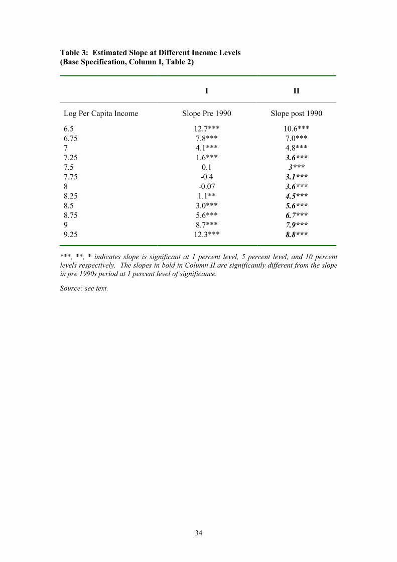
In Table 3 we calculate the slope of services as a share in GDP with respect to per
capita income based on the coefficients in column IV, Table 1, at different income
levels. The slopes indicate that in 1950-1989 the service sector’s share of GDP first
rose with per capita income before stabilizing at middle incomes. Note that a log per
capita GDP of 7.5, where this stagnation sets in, is approximately 1800 U.S. year
2000 purchasing-power-parity dollars. Then at still higher income levels the service
sector’s share of GDP starts rising again. Here a log per capita income of 8.25, where
this second wave of service-sector growth becomes apparent, corresponds to
approximately US $3825. Since we detect this pattern in the data for 1950-1989, it
does not appear that the second wave of service sector growth is exclusively a post-
1990s phenomenon.8
7 Specifically we drop observations with per capita income in the bottom 10 percent, which corresponds to observations below log per capita income level 6.65 or income level of 770 year 2000 US purchasing-power-parity dollars. Examples of countries below this threshold are Tanzania, Malawi, Madagascar, Uganda and Rwanda.
8 Starting in the 1990s, it would appear, the relationship became steeper everywhere other than high income levels – that is, at log per capita incomes above 8.75 (a log per capita income of 8.75
7
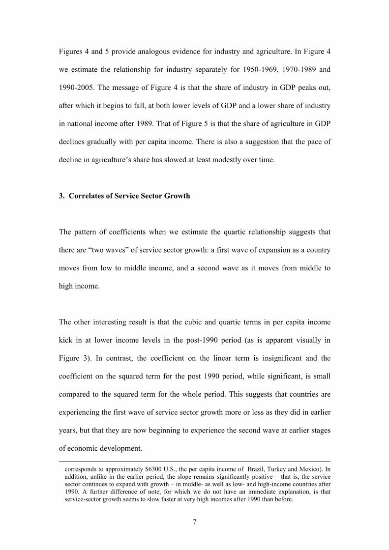
Figures 4 and 5 provide analogous evidence for industry and agriculture. In Figure 4
we estimate the relationship for industry separately for 1950-1969, 1970-1989 and
1990-2005. The message of Figure 4 is that the share of industry in GDP peaks out,
after which it begins to fall, at both lower levels of GDP and a lower share of industry
in national income after 1989. That of Figure 5 is that the share of agriculture in GDP
declines gradually with per capita income. There is also a suggestion that the pace of
decline in agriculture’s share has slowed at least modestly over time.
3. Correlates of Service Sector Growth
The pattern of coefficients when we estimate the quartic relationship suggests that
there are “two waves” of service sector growth: a first wave of expansion as a country
moves from low to middle income, and a second wave as it moves from middle to
high income.
The other interesting result is that the cubic and quartic terms in per capita income
kick in at lower income levels in the post-1990 period (as is apparent visually in
Figure 3). In contrast, the coefficient on the linear term is insignificant and the
coefficient on the squared term for the post 1990 period, while significant, is small
compared to the squared term for the whole period. This suggests that countries are
experiencing the first wave of service sector growth more or less as they did in earlier
years, but that they are now beginning to experience the second wave at earlier stages
of economic development.
corresponds to approximately $6300 U.S., the per capita income of Brazil, Turkey and Mexico). In addition, unlike in the earlier period, the slope remains significantly positive – that is, the service sector continues to expand with growth – in middle- as well as low- and high-income countries after 1990. A further difference of note, for which we do not have an immediate explanation, is that service-sector growth seems to slow faster at very high incomes after 1990 than before.

8
To understand where and why, we first identify correlates which when interacted with
the four terms in per capita income reduce or eliminate the significance of all four per
capita income terms. These are the factors that appear to be associated with our two
waves. The variables we consider as potential correlates include the size of the
economy (GDP), openness to trade (as measured by the trade-to-GDP ratio), openness
to trade in services (as measured by trade-in-services-to-GDP ratio); and vector of
demographic, geographical and political variables (including democracy, latitude,
share of land area in the tropics, the dependency ratio (both youth and old age), and
proximity to the major economic and financial centers).9 Some of these explanatory
variables are highly correlated with each other and with per capita income, as shown
in Table 4. The overall trade and trade in services ratios are highly correlated, for
example. Latitude and area in the tropics are obviously correlated. For this reason we
do not always include all potential explanatory variables in all equations.
We use a general to specific approach. We start with a very general specification and
then drop variables with insignificant coefficients. In this way we obtain a
parsimonious specification.
In these parsimonious regressions the coefficients of the per capita income terms are
not significantly different from zero—implying that the two waves of service sector
growth are being driven by the factors included in the parsimonious regressions. We
9 Data on trade in services begins only around 1970 for some countries in our sample. Availability improves over the years and by 1975 data are available for about half the countries, and by 1980 for 80 percent of the countries in the sample; therefore regressions including this variable have been estimated on fewer observations. The remaining variables are either time invariant or vary little. The geographical variables are, of course, time invariant, while democracy, age dependency, and literacy vary over time but show considerable persistence.

9
have estimated these regressions first including total trade, and then including trade in
services. We first report results for total trade in Table 5.
In Column I we include all of the potential explanatory variables interacted with the
four per capita income terms. In Column II we drop the variables interacting urban
population with per capita income; in Column III we drop the terms interacting
governance with per capita income; in Column IV we drop the terms interacting age
dependency with per capita income; and in Column V we drop the terms interacting
area outside the tropics with per capita income.
While more urban countries have larger service sectors, the four powers of
urbanization are generally insignificant; urbanization does not appear to be explaining
the two-wave pattern in other words. In contrast, in countries more open to trade,
more democratic, and closer to the major financial centers, the four powers of per
capita income tend to be insignificantly different from zero in most specifications.10
Some specifications also suggest a role for physical geography (share of land area in
outside the tropics). Importantly, the four powers of per capita income are now
insignificantly different from zero.11 It would appear that these variables suffice to
explain the two wave pattern.
In order to interpret the coefficients, we calculate the slope of our dependent variable
with respect to income at various income levels and at various values of the
10 This last result is not driven by Western Europe and Canada. When we drop these countries from the sample, the terms involving minimum distance still have significant coefficients. Note that the significance of the trade variable is evident only in the more parsimonious specifications.
11 They remain statistically significant as a group, which is telling us that per capita income still matters for the size of the service sector (richer countries have larger service sector shares), but no longer for the two-wave pattern.

10
explanatory variables. For example, taking the coefficients in Column V in Table 5,
we can compute the slopes at three sets of values for trade, distance from the major
financial center and democracy: low, medium and high (respectively values at the
bottom quartile, median and the top quartile of these variables). Estimated slopes for
the low, medium and high values of these variables at various income levels are
presented in Table 6.
At low values of trade, democracy and proximity, we do not see a second wave of
service sector growth – that is to say, the services share does not begin increasing
again with per capita income above middle income levels. In contrast, at high values
of these three variables we see the slope again becoming positive at higher income
levels. This supports our conclusion that the second wave of service sector growth is
observed in countries which are more open, more democratic and closer to the major
global financial centers.
These results withstand a number of robustness checks. We include year dummies
rather than the dummies for 1970-1989 and 1990-2005; cluster the standard errors by
country and alternatively by year (to allow for standard errors to be correlated across
years within each country; and to allow the standard errors to be correlated across
countries in each year). We also add back in the variables dropped in the earlier stages
(urbanization, age dependency or governance), interacting them with the four powers
of per capita income. When we include these in our parsimonious specification, the
coefficients of these variables remain insignificant, and their inclusion does not affect
the coefficients on the trade, democracy and proximity-to-financial-center terms.12
12 Or the coefficients on the powers of per capita income.

11
Table 7 substitutes trade in services for total trade.13 Trade in services is significant in
all specifications. Otherwise the results are essentially the same as before, except that
there is less support for the importance of climate. We conclude that openness to trade
in services, democracy and proximity to the major financial centers are drivers of the
two-wave pattern.
Next we ask whether any of the variables considered so far can explain the shift in the
relationship in the services/GDP ratio since 1990. The equations in Table 8 now
include all four terms in PCY; these four terms interacted with the post 1990 dummy;
dummies for 1970-1989 and for 1990-2005; other potential explanatory variables
interacted with PCY terms; and the latter interacted with the post 1990 dummy.
In Column I of Table 8 (which reproduces Column IV of Table 1 as a benchmark), the
coefficients on per capita income interacted with the post-1989 dummy are all
significant. In Column II we include additional variables affecting the size of the
service sector: GDP, urban population, trade, democracy. The coefficients on per
capita income and interaction with the dummy variable for the post-1990 period do
not change. This means that these variables by themselves cannot explain the post-
1989 shift in the pattern of service sector growth.
In column III we add variables explaining the two wave pattern of growth:
democracy, trade and proximity to financial centers interacted with the powers of per
capita income. These variables seem to explain the first as well as the second wave of
service sector growth in pre-1990 period but not subsequently.
13 The general-to-specific procedure and the sequence in which we dropped insignificant variables remain the same.

12
In column IV we interact trade, democracy, and proximity with per capita income as
well with as the post-1990 dummy. Now the coefficients of the per capita income
terms interacted with post 1990s dummy are no longer significantly different from
zero. In column V we drop trade interacted with per capita income terms and the post-
1989 dummy, since the coefficients on the trade variables were insignificant in
column IV.
The results suggest that democracy, proximity to major financial centers and trade
openness explain the post-1990 shift in the share of services in GDP, in that they
make the significance of the per-capita-income-post-1990 interaction go to zero.
We can again calculate the slope of the share of services in GDP with respect to per
capita income at various income levels in the pre- and post-1990 periods for different
values of the explanatory variables, as in Table 9. We continue to see in Columns I-IV
our two-wave pattern of service sector growth, with a second wave at middle and high
incomes only in countries with relatively high levels of trade, democracy, and
proximity to the major financial centers. These variables also seem to be associated
with the shift in services income relationship after 1989, although that shift now does
not seem especially pronounced.
When we include trade, democracy, and proximity interacted with per capita income,
as well as per capita income and the post 1990s dummy, we can explain the shift in
the services/GDP since 1990s better (slopes not shown in Table 9). Finally, in order to
improve the fit of the regression, we drop the interaction of trade and the post 1990s
dummy, thus allowing for the possibility that trade did not have a differential impact

13
on the services and per capita income relationship post 1990s. The slopes calculated
using this specification are reported in Columns V-VIII in Table 9. Now the second
wave occurs only in countries with relatively high levels of trade, democracy, and
proximity to the major financial centers; and the post-1990 shift is more pronounced
in countries with these features.
4. Country-Specific Experience
We now examine how growth of the service sector in individual countries compares
with the typical pattern in different sub-periods.14 The data for the United States are
highlighted in Figure 6. The size of the service sector is more or less as predicted in
the 1970s and 1980s. In the 1990s it then grows significantly larger than predicted
even for a high income country. In other words, the U.S. observations lie entirely
above the two-standard-error bands. This story is well known: it reflects the
productivity-enhancing restructuring of retail, wholesale and financial services,
enabled by the application of new information technology; in part it reflects rapid
deregulation and unsustainable growth of the financial services industry.
Japan was known in the third quarter of the 20th century for having a manufacturing-
heavy economy. In Figure 7 we see that the service share of GDP was not, in fact,
atypical in the 1960s. The period when the service-sector share is smaller than
expected was the 1970s and 1980s (mainly the early 1970s and late 1980s). There was
then convergence to the international norm after 1990, with relatively rapid growth in
the output shares of business, health and social services.
14 The typical pattern is given in Figure 3 above, where we plot the predicted services/share in different time periods and along with their two standard error bands.

14
In contrast, Germany, another traditionally manufacturing-heavy country, shows
evidence in Figure 8 of having had an unusually low service-sector share in the 1950s
and 1960s, the decades of the manufacturing Wirtschaftswunder. This anomaly
disappeared in the 1970s and 1980s. In recent years, the service sector grew unusually
rapidly by international standards, perhaps reflecting deindustrialization in the new
eastern lander.15 By the end of the sample period there is some sign of a service-
sector share slightly higher than expected.
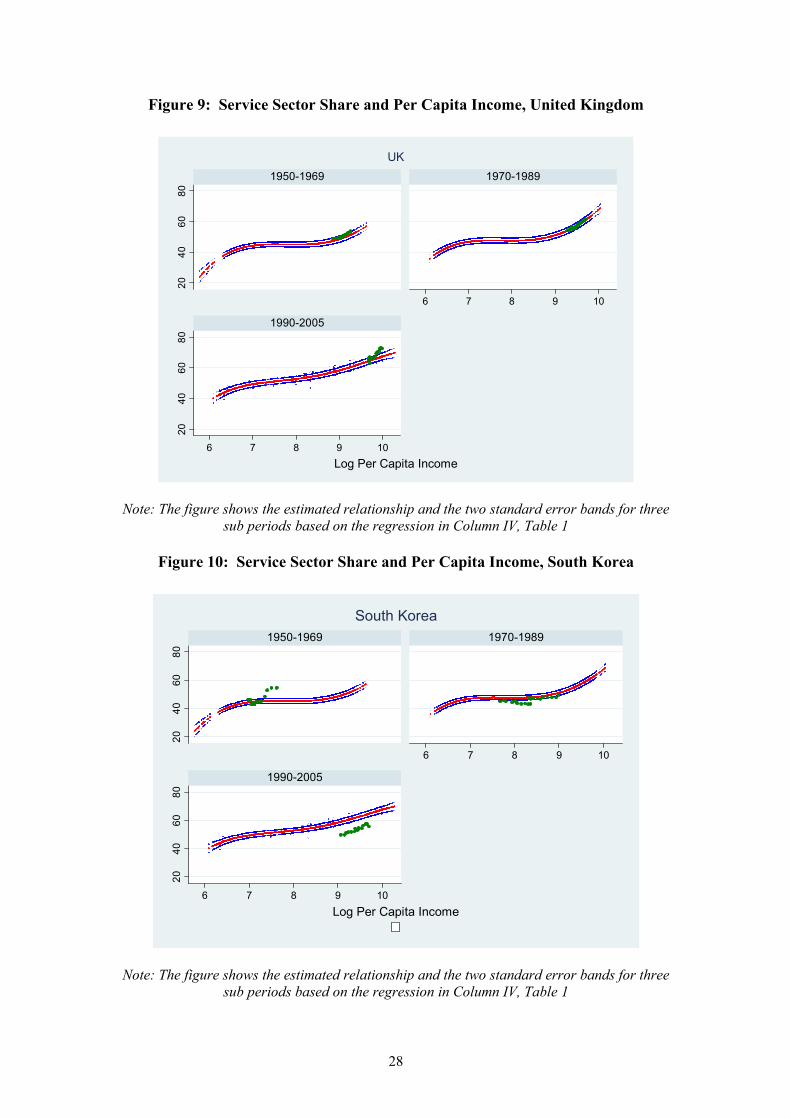
Figure 9 for the UK suggests that the service sector share was typical for a country
with its per capita GDP from the 1950s through the 1980s, notwithstanding the debate
over the country’s deindustrialization (which would lead one to expect a service
sector significantly larger than the international norm). Then in the 1990s the service
sector becomes unusually large by the standards of that international norm.
Interestingly, unusually large subsectors include not only financial services but also
retail trade, legal, technical, legal and other community, social and personal
services.16
Finally, Figure 10 considers a late-developing middle-income country, Korea. The
fact that Korea has a relatively underdeveloped service sector characterized by low
productivity is well known: OECD (2008) observes that the productivity gap vis-à-vis
other OECD countries is much larger for services than manufacturing, a problem that
can be ascribed in large part to restrictive regulations designed to protect small and
medium-sized enterprises from domestic and foreign competition. Figure 10 suggests
that the problem of a stunted service sector is relatively recent. It was barely visible in
15 Which is of course not included in the data for the earlier period. 16 According to the EU KLEMS data base, described further below.

15
the 1970s and 1980s but emerges clearly in the 1990s,when the typical relationship
between the service-sector share of output and per capita income shifts up but Korea
lags behind. This may reflect Korea’s lack of proximity to the major global financial
centers, New York and London, and difficulty of establishing itself as a financial hub
for Northeast Asia.
5. Traditional and Modern Services
Direct evidence on the composition of service sector production at different income
levels can be constructed mainly for high-income countries on the basis of data
provided by the EU KLEMS project for the period 1970-2005. The limitations of the
data limit the analysis: we cannot analyze the compositional sources of the pre/post-
1970 shift, for example, or examine what has been going on in low-income countries.
The EU KLEMS release of 2008 spans the period 1970-2005 for the 15 founding
(pre-2004) EU member states and for the US, South Korea, Japan and Australia.
Series from 1995 onwards are available for the new EU member states which joined
the EU on 1 May 2004. Industries are classified according to the European NACE
revision 1 classification, but the level of detail varies across countries, industries and
variables owing to differences in national statistical procedure. For our analysis we do
not include the new member states and further drop Luxembourg and Portugal.17 Thus
we use the data on Australia, Austria, Belgium, Denmark, Finland, France, Germany,
Greece, Ireland, Italy, Japan, Korea, Netherlands, Spain, Sweden, United Kingdom,
and United States in the disaggregated analysis. We calculate the share of different
17 Where there are data-availability problems.

16
services in GDP using value added at current prices in local currency for various
service industries and total GDP.18
We distinguish three groups of services according to whether their shares of GDP
have fallen, risen slowly, or risen rapidly over time. First are traditional services:
retail and wholesale trade, transport and storage, public administration and defense.
Their share in GDP has fallen noticeably over time. The second group is a hybrid of
traditional and modern services consumed mainly by households: education; health
and social work; hotels and restaurants; and other community, social and personal
services. Their shares all show a tendency to rise slowly with time. The third group is
modern services consumed by both the household and corporate sectors: financial
intermediation, computer services, business services, communication, and legal and
technical services. We refer to them as modern because their share in GDP was a
negligible 7 per cent in 1970, since when it has risen to more than 15 percent. Details
on these three groups are in Table 10.
The quartic relationship between the share of services in GDP and per capita income
is still evident in this smaller sample, although it is not as pronounced as in the larger
sample of low- and middle- as well as high-income countries.19 Figures 12-14 show
the fitted values for our three groups. That the GDP share of services such as public
18 We also use the data on total factor productivity from the EU KLEMS. Certain services that were very small or did not seem to be following any specific pattern of growth are excluded. One sector which is relatively large that we did not include is real estate activities (8 percent). Real estate services seem to be quite volatile and do not fit any neat pattern of growth. This could be due to the fact that valuation of these services changes with real estate prices and these are not adequately accounted for in the real prices. We also test the robustness of results to including these services in different groups, where they seem to be fitting e.g. activities related to financial intermediation in group III with financial intermediation; sale, maintenance and repair of motor in Group I with retail trade; and private households with personal services in group II. The results are robust.
19 There are also some signs of a shift in the relationship after 1990, but this too is small in comparison with the larger sample of countries.

17
administration and defense, retail trade, wholesale trade and transport and storage
(Group I), declines steadily as countries move from middle- to high-income status,
consistent with a low income elasticity of demand for these services, is not in conflict
with the existence of a hump-shaped pattern, since here we do not observe the share
of Group I in low-income countries.
As shown in Figure 13, the share of Group II services grows faster than the rest of the
economy all through the middle- and high-income range. This behavior is consistent
with a high income elasticity of demand.
Finally, for Group III, we see an increase in their GDP share over the entire range of
middle- and high-income levels. The share of these activities increases particularly
rapidly at high incomes, with no sign (in contrast to Group II) of that share growing
more slowly at the high end, indicating very high income elasticities of demand and
or the greater tradability and therefore capacity to export these services. Although we
do not observe the share of such modern services in low income countries it seems
safe to conjecture that the importance of Group III rises steadily with per capita
income.
Having considered demand, we look also at some potential determinants of the supply
of these services. Productivity growth was highest, not surprisingly, in the Group III
modern services (Table 11). Interestingly, however, productivity increases have also
been relatively rapid within traditional services (Group I), some of which (retailing,
wholesaling) have made extensive use of new information technologies. This
reinforces the presumption that insofar as the share of output accounted for by Group

18
I has declined, this reflects relatively low income elasticities of demand. It is in Group
II, the hybrid cases, where the cost disease appears to be most serious. Suggestively,
Group II ranks lowest in terms of the penetration/application of new information
technology. It also has the lowest international tradability, suggesting that limits on
international competition and on the ability to specialize contribute to this problem.20
6. Conclusion
We have provided new evidence and analysis of the share of services in GDP in the
course of economic development. We identify two waves of service sector growth, a
first wave in countries with relatively low levels of per capita GDP and a second wave
in countries with higher per capita incomes. The first wave appears to be made up
primarily of traditional services, the second wave of modern (financial,
communication, computer, technical, legal, advertising and business) services that are
receptive to the application of new information technology and increasingly tradable
across borders.
There is evidence of an increase in the share of services in GDP at all levels of
income after 1970 and, in addition, of a further increase in the share of services in
20 The indicator of tradability is constructed using data in Jensen and Kletzer (2005). Since Jensen and Kletzer work with the NAICS (North American Industrial classification system), we map their classification into our NACE (European Classification of Economics Activities). Jensen and Kletzer calculate the Gini Coefficient for the geographical dispersion of each activity and use it to identify tradable and non tradable services. The underlying idea is that the services which are tradable can be geographically concentrated in order to reap the economies of scale. The mapping was quite clear for all of our services except for Transport and storage. Two different NAICS codes are assigned to these activities, each with a different degree of tradability. Hence we leave this cell blank. Another case where the tradability was not clear is the wholesale trade. For this service category Jensen and Kletzer find it to be having an almost equal score for tradability and non tradability. Indicators for information and communication technology (ICT) industries has been constructed using the data in van Ark, Inklaar and McGucken (2005).

19
countries with relatively high per capita incomes – in other words, of the second wave
occurring at lower income levels than before. But this change in the second wave is
not equally evident in all countries: it is most apparent in countries that are open to
trade, that are democratic, and that are relatively close to the major global financial
centers. This points to both political and economic conditions that can help countries
capitalize on the opportunities afforded by am increasingly globalized post-industrial
economy.

20
References
Buera, Francisco J. and Joseph P. Kaboski (2008), “Scale and Origins of Structural Change,” unpublished manuscript.
Buera, Francisco J. and Joseph P. Kaboski (2009), “The Rise of the Services
Economy,” NBER Working paper 14822. CEPII database, 2008, http://www.cepii.fr/anglaisgraph/bdd/bdd.htm. Chenery, Hollis (1960), “Patterns of Industrial Growth,” American Economic Review
50, pp 624-654. Chenery, Hollis and Moshe Syrquin (1975), Patterns of Development, 1957-1970,
Oxford: Oxford University Press. Clark, Colin (1940), The Conditions of Economic Progress, London: Macmillan.
EU KLEMS Database (2007), EU LEMS Growth and Productivity Accounts,
http://www.euklems.net. Fisher, A.G.B. (1939), “Primary, Secondary and Tertiary Production,” Economic
Record 15, pp.24-38. Gallup, John Luke and Jeffrey D. Sachs, and Andrew Mellinger (1999), “Geography
and Economic Development.” CID Working Paper No. 1, Center for International Development, Harvard University.
Jensen, Bradford J. and Lori G. Kletzer, 2005, “Tradable Services: Understanding the
Scope and Impact of Services Outsourcing,” Institute for International Economics Working Paper No. 05-9.
Kongsamut, Piyabha, Sergio Rebelo and Danyang Xie (1999), “Beyond Balanced
Growth,” NBER Working Paper 6159. Kuznets, Simon (1957), “Quantitative Aspects of the Economic Growth of Nations:
II, Industrial Distribution of National Product and Labor Force,” Economic Development and Cultural Change, Vol. 5, No. 4, (supplement), pp.1-111.
Kuznets, Simon (1973), “Modern Economic Growth: Findings and Reflections,”
American Economic Review 63, pp. 247-258. Maddison, Angus (2003), “Historical Statistics for the World Economy: 1-2003 AD,
downloaded from http://www.ggdc.net Mitchell B. R. (1982), International Historical Statistics-Asia and Africa, New York:
New York University Press

21
Mitchell B. R. (1992), International Historical Statistics-Europe 1750-1988, New York: Stockton Press.
Mitchell B. R. (1993), International Historical Statistics-The Americas, New York:
Stockton Press. OECD (2008), Korea Economic Survey, Paris: OECD. Polity (various years), Polity IV Data Base: Political Regime Characteristics and
transitions, 1800-2007. Van Ark, Bart, Robert Inklaar and Robert H. McGuckin, 2003. "ICT and Productivity
in Europe and the United States: Where Do the Differences Come From?" Economics Program Working Papers 03-05, Washington, D.C.: The Conference Board
World Bank (various years), World Development Indicators, Washington, D.C.:
World Bank.

22
Appendix
Table A 1: Data Sources and Construction of Variables
Sources Definitions
Sectoral shares in GDP (agriculture, industry and services)
WDI, Mitchell (various editions)
Shares of agriculture, industry and services in GDP (in percent)
Per capita income Maddison, WDI Per capita income in 2000 PPP US $, Maddison and WDI
GDP Maddison, WDI GDP in 2000 PPP US $, Maddison and WDI
Trade/GDP WDI, Mitchell, Penn World Tables
(Export + Import of goods and services)/GDP, in percent
Trade in services WDI (Export + Import of services)/GDP, in percent
Distance CEPII Great Circle distance between capital cities and either the US or the UK, whichever is smaller, in Kilometer
Latitude Gallup, Sachs and Mellinger
latitude
Urban Population WDI
Urban population (% of total Population)
Age dependency WDI Share of dependents to working-age population
Non tropical area Gallup, Sachs and Mellinger
Percentage of land outside the tropics.
Governance World Bank, Aggregate Governance Indicators 1996-2007
The average of governance indicators measured in units ranging from about -2.5 to 2.5, with higher values corresponding to better governance outcomes.
Democracy Polity IV Institutionalized Democracy Score, takes values between 0 and 10

23
Table A 2: Summary Statistics
Variable Number of
Observations
Mean Std. Dev. Min Max
Services/GDP (in percent) 3950 50.2 11.1 18.4 77
Log Per Capita Income 3937 8.1 1.1 5.8 10.3
Log GDP 3877 10.6 1.92 5.37 15.9
Trade (percent of GDP) 3838 56.5 33.3 2.7 251.1
Urban Population(percent of total)
3415 49.1 24.1 2.4 97.3
Democracy 3674 5.31 4.3 0 10
Trade in Services (percent of GDP)
2358 14.5 9.5 0 82.8
Distance from Major Financial centers
3931 5118 3689 0 15958
Governance 3950 0.23 0.99 -1.45 1.95
Non tropical area (Share of total area)
3850 0.55 0.47 0 1
Latitude 3950 27.7 17.2 1.2 63.5
Age dependency (share of working population)
3415 0.74 0.20 0.39 1.13

24
Figure 1: Lowess Plot of the Relationship between Log Per Capita Income and
Services/GDP
20
30
40
50
60
70
(Serv
ices/G
DP
)
6 7 8 9 10Log Per Capita Income
1950-1969 1970-1989
1990-2005
Figure 2: Log Per Capita Income and Services/GDP
Based on Quartic Function Estimation
(Different Slopes in the Three Subperiods)
20
30
40
50
60
70
Lin
ear
pre
dic
tion
6 7 8 9 10Log Per Capita Income
1950-1969 1970-1989
1990-2005
Note: Based on regression in Column III, Table 1

25
Figure 3: Log Per Capita Income and Services/GDP, Quartic Estimation
(Different Slopes in 1950-1989 and 1990-2005)
20
30
40
50
60
70
Lin
ear
pre
dic
tion
6 7 8 9 10Log Per Capita Income
1950-1969 1970-1989
1990-2005
Note: Based on regression in Column IV, Table 1.
Figure 4 : Lowess Plot for Log Per Capita Income and Share of Industry in GDP
10
20
30
40
Industr
y/G
DP
6 7 8 9 10Log Per Capita Income
1950-1969 1970-1989
1990-2005

26
Figure 5 : Lowess Plot for Log Per Capita Income and Share of Agriculture in
GDP
020
40
60
Agriculture
/GD
P
6 7 8 9 10Log Per Capita Income
1950-1969 1970-1989
1990-2005
Figure 6: Service Sector Share Per Capita Income, United States
20
40
60
80
20
40
60
80
6 7 8 9 10
6 7 8 9 10
1950-1969 1970-1989
1990-2005
Log Per Capita Income
USA
Note: The figure shows the estimated relationship and the two standard error bands for three
sub periods based on the regression in Column IV, Table 1

27
Figure 7: Service Sector Share and Per Capita Income, Japan
20
40
60
80
20
40
60
80
6 7 8 9 10
6 7 8 9 10
1950-1969 1970-1989
1990-2005
Log Per Capita Income
Japan
Note: The figure shows the estimated relationship and the two standard error bands for
three sub periods based on the regression in Column IV, Table 1.
Figure 8: Service Sector Share and Per Capita Income, Germany
20
40
60
80
20
40
60
80
6 7 8 9 10
6 7 8 9 10
1950-1969 1970-1989
1990-2005
Log Per Capita Income
Germany
Note: The figure shows the estimated relationship and the two standard error bands for three
sub periods based on the regression in Column IV, Table 1.
28
Figure 9: Service Sector Share and Per Capita Income, United Kingdom
20
40
60
80
20
40
60
80
6 7 8 9 10
6 7 8 9 10
1950-1969 1970-1989
1990-2005
Log Per Capita Income
UK
Note: The figure shows the estimated relationship and the two standard error bands for three
sub periods based on the regression in Column IV, Table 1
Figure 10: Service Sector Share and Per Capita Income, South Korea
20
40
60
80
20
40
60
80
6 7 8 9 10
6 7 8 9 10
1950-1969 1970-1989
1990-2005
Log Per Capita Income
South Korea
Note: The figure shows the estimated relationship and the two standard error bands for three
sub periods based on the regression in Column IV, Table 1

29
Figure 11: Estimated Relationship between the Share of the Services and Per
Capita Income for the EU KLEMS Sample
40
50
60
70
80
Estim
ate
d s
er/
va f
or
EU
KLE
MS
sam
ple
7 8 9 10 11Log Per Capita Income
Note: The figure shows the estimated quartic relationship between services/GDP and log per
capita income for the sample included in the EUKLEMS database
Figure 12: Estimated Relationship Between the Share of Group I Services and
Per Capita Income
20
25
30
35
Estim
ate
d S
ize
7 8 9 10 11Log Per Capita Income
Note: Group I includes public administration and defense, retail trade, wholesale
trade, and transport and storage. The estimated values are based on a regression
of share of services in GDP for activities belonging to this group on four terms of
per capita income and country-service fixed effects.

30
Figure 13: Estimated Relationship Between the Share of Group II Services and
Per Capita Income
810
12
14
16
18
Estim
ate
d S
ize
7 8 9 10 11Log Per Capita Income
Note: Group II includes education, hotels and restaurants, Health and social work, and other
community social and personal services. The estimated values are based on a regression of
share of services in GDP for activities belonging to this group on four terms of per capita
income and country-service fixed effects.
Figure 14: Estimated Relationship Between the Share of Group III Services and
Per Capita Income
05
10
15
20
Estim
ate
d S
ize
7 8 9 10 11Log Per Capita Income
Note: Group III includes computer, legal, technical and advertising, financial intermediation,
other business services and post and telecommunication. The estimated values are based on a
regression of share of services in GDP for activities belonging to this group on four terms of
Per capita income and country-service fixed effects.

31
Figure 15: Estimates Shares for Group III Subsectors
01
23
4E
stim
ate
d C
om
pute
r A
ctivitie
s
7 8 9 10 11log PCY
Computer and related Activities
01
23
4E
stim
ate
d P
ost_
Com
munic
ation
7 8 9 10 11log PCY
Post and Communication
12
34
56
Estim
ate
d L
egal and T
echnic
al A
ctivitie
s
7 8 9 10 11log PCY
Legal and Technical Activities
23
45
67
Estim
ate
d F
ina
ncia
l A
ctivitie
s
7 8 9 10 11log PCY
Financial intermediation
-10
12
3E
stim
ate
d O
ther
Bus A
ctivitie
s
7 8 9 10 11log PCY
Other Business Activity

32
Table 1: Quartic Relationship Between Log Per Capita Income and Share of
Services in GDP [Dependent Variable: Services/GDP (in percent)]
I II III IV
Log Per Capita Income 1,000.6*** 1,518.2*** 661.2** 830.3*** [5.64] [8.09] [2.30] [4.02] Log Per Capita Income, squared -171.6*** -271.1*** -94.3* -132.9*** [5.17] [7.75] [1.66] [3.40] Log Per Capita Income, cube 12.9*** 21.2*** 5.2 9.05*** [4.69] [7.37] [1.05] [2.77] Log Per Capita Income, quartic -0.35*** -0.61*** -0.07 -0.22** [4.16] [6.95] [0.47] [2.11] Dummy for 1970-1989 2.41*** 83.8 2.5*** [10.36] [0.12] [10.66] Dummy for 1990-2005 6.9*** 88.26 48.2 [21.96] [0.68] [0.39] Log Per Capita Income *dummy-1970-1989
-32.71
[0.09] Log Per Capita Income squared* dummy-1970-1989
3.47
[0.05] Log Per Capita Income, cube* dummy-1970-1989
0.03
[0.01] Log Per Capita Income, quartic* dummy-1970-1989
-0.01
[0.08] Log Per Capita Income *dummy-1990-2005
49.18 46.46
[0.79] [0.76] Log Per Capita Income, squared* dummy-1990-2005
-28.58** -22.72*
[2.21] [1.93] Log Per Capita Income, cube* dummy-1990-2005
4.15*** 3.13***
[3.19] [3.00] Log Per Capita Income, quartic* dummy-1990-2005
-0.19*** -0.14***
[3.79] [3.88] Country Fixed effects yes yes yes yes Observations 3937 3937 3937 3937 Number of Countries 91 91 91 91 R-squared 0.81 0.84 0.84 0.84
Note: Robust t statistics are in parentheses. *, **, *** indicate coefficient is significant at 10,
5, and 1 percent levels respectively. Column 1 shows the quartic relationship with a common
intercept for all years. Column II allows the intercepts to differ in 1970-1989 and in 1990-
2005. Column III allows the coefficients on log per capita income terms to differ in 1950-69,
1970-1989 and 1990-2005 subperiods. Column IV allows the coefficients on log per capita
income terms to differ in 1950-89, and 1990-2005 subperiods. Source: see text.

33
Table 2: Relationship Between Log Per Capita Income and Services/GDP: Robustness Checks [Dependent Variable: Services/GDP (in percent)]
I II III IV
Dummy for 1970-1989 2.53*** 2.54*** 2.40*** [10.66] [10.46] [10.25] Dummy for 1990-2005 48.23 201.22 50.11 [0.39] [1.44] [0.41] Log Per Capita Income 830.3*** 2,641.4*** 785.4*** 1,194.5*** [4.02] [7.47] [3.89] [5.18] Log Per Capita Income, squared -132.9*** -458.6*** -123.9*** -204.3*** [3.40] [7.05] [3.24] [4.70] Log Per Capita Income,cube 9.05*** 34.95*** 8.27*** 15.17*** [2.77] [6.60] [2.59] [4.20] Log Per Capita Income, quartic -0.22** -0.98*** -0.19* -0.41*** [2.11] [6.12] [1.91] [3.67] Log Per Capita Income *dummy-1990-2005 46.46 8.15 47.24 37.28 [0.76] [0.13] [0.78] [0.63] Log Per Capita Income squared*dummy-1990-2005 -22.7* -21.7* -23.2** -20.1* [1.93] [1.76] [2.00] [1.75] Log Per Capita Income, cube* dummy-1990-2005 3.13*** 3.46*** 3.19*** 2.84*** [3.00] [3.13] [3.11] [2.78] Log Per Capita Income,quartic* dummy-1990-2005 -0.14*** -0.16*** -0.14*** -0.13*** [3.88] [4.12] [4.01] [3.62] Country Fixed Effects Yes Yes RE Yes Observations 3937 3544 3937 3937 Number of Countries 91 87 91 91 R-squared 0.84 0.85 0.86
Note: Robust t statistics in parentheses. *, **, *** indicate coefficient is significant at 10, 5, and 1 percent levels respectively. Column I shows the base specification (same
as in Column IV, Table1). Column II drops the observations with log income levels below 6.65, income level below $770. Column III is Random effects specification.
Column IV includes annual dummies rather than dummies for different time periods. Source: see text.
34
Table 3: Estimated Slope at Different Income Levels
(Base Specification, Column I, Table 2)
I II
Log Per Capita Income
Slope Pre 1990
Slope post 1990
6.5 12.7*** 10.6***
6.75 7.8*** 7.0***
7 4.1*** 4.8***
7.25 1.6*** 3.6***
7.5 0.1 3***
7.75 -0.4 3.1***
8 -0.07 3.6***
8.25 1.1** 4.5***
8.5 3.0*** 5.6***
8.75 5.6*** 6.7***
9 8.7*** 7.9***
9.25 12.3*** 8.8***
***, **, * indicates slope is significant at 1 percent level, 5 percent level, and 10 percent
levels respectively. The slopes in bold in Column II are significantly different from the slope
in pre 1990s period at 1 percent level of significance.
Source: see text.

35
Table 4 : Correlation Matrix
PCY GDP Trade Urban
Pop
Democ-
racy
Trade,
Services
Proximity
Financial
Centers
Gover-
nance
Non
Tropical
Area
Latitude
Log PCY
1
Log GDP 0.64* 1
Trade 0.18* -0.28* 1
Urban Population 0.86* 0.54* 0.14* 1
Democracy 0.66* 0.45* 0.09* 0.58* 1
Trade in Services 0.01 -0.43* 0.73* 0.03 -0.05 1
Proximity Major Financial Centers
0.41* 0.21* 0.11* 0.39* 0.32* 0.15* 1
Governance 0.78* 0.49* 0.11* 0.67* 0.65* 0.05* 0.36* 1
Non Tropical Area 0.61* 0.54* -0.03 0.59* 0.37* -0.02 0.42* 0.69* 1
Latitude 0.71* 0.47* 0.09* 0.63* 0.51* 0.02 0.53* 0.79* 0.88* 1
Age Dependency -0.79* -0.66* -0.15* -0.71* -0.62* 0.04 -0.31* -0.72* -0.64* -0.69*
* Indicates the correlation coefficient is significant at 1 percent level of significance
Source: see text

36
Table 5: Explaining the Pattern of Service Sector Growth
[Dependent Variable: Services/GDP (in percent)]
I II III IV V Dummy for 1970-1989 -0.02 0.21 -0.09 -0.01 -0.12 [0.05] [0.73] [0.31] [0.02] [0.43] Dummy for 1990-2005 2.78*** 3.08*** 2.85*** 3.12*** 2.76*** [5.93] [6.68] [6.16] [6.87] [6.16] Log Per Capita Income (PCY) 336.3 -1,932.9* -1,059.1 -583.1 620.2 [0.29] [1.75] [1.07] [0.59] [0.69] Log Per Capita Income, square 31.9 496.2** 332.4* 210.1 -41.3 [0.14] [2.34] [1.73] [1.13] [0.24] Log Per Capita Income,cube -9.95 -51.4*** -37.8** -25.48 -2.56 [0.52] [2.81] [2.26] [1.62] [0.18] Log Per Capita Income, quartic 0.52 1.89*** 1.46*** 1.03** 0.26 [0.85] [3.18] [2.67] [2.07] [0.56] Log GDP 2.61*** 1.55** 1.62** 1.68** 1.61** [3.30] [2.21] [2.29] [2.36] [2.30] Trade (% of GDP) -4.54 -20.08 -13.38 -22.3 -39.42** [0.21] [0.98] [0.69] [1.22] [2.31] Urban Population (% of total Population)
17.93 0.14*** 0.15*** 0.15*** 0.16***
[0.53] [4.89] [5.26] [5.25] [5.79] Trade *Log PCY 4.92 12.41 9.11 13.54 21.65*** [0.46] [1.24] [0.96] [1.51] [2.59] Trade*log PCY squared -1.37 -2.71 -2.11 -2.92* -4.35*** [0.71] [1.49] [1.22] [1.79] [2.85] Trade*log PCY cube 0.15 0.25* 0.2 0.27** 0.38*** [0.95] [1.73] [1.46] [2.05] [3.10] Trade*log PCY quartic -0.01 -0.01* -0.01* -0.01** -0.01*** [1.18] [1.95] [1.70] [2.29] [3.32] Democracy -662** -522** -637*** -571*** -561*** [2.47] [2.16] [3.21] [3.15] [3.67] Democracy* log PCY 342.5** 267.2** 331.5*** 298.1*** 292.8*** [2.46] [2.13] [3.23] [3.17] [3.69] Democracy*log PCY square -65.9** -50.8** -64.2*** -57.96*** -56.95*** [2.44] [2.09] [3.23] [3.19] [3.70] Democracy*log PCY cube 5.59** 4.25** 5.48*** 4.97*** 4.89*** [2.41] [2.04] [3.21] [3.19] [3.68] Democracy*log PCY quartic -0.18** -0.13** -0.17*** -0.16*** -0.16*** [2.37] [1.98] [3.18] [3.17] [3.65] Proximity*PCY 0.45*** 0.50*** 0.49*** 0.54*** 0.57*** [5.34] [6.37] [6.37] [7.06] [8.03] Proximity*PCY square -0.08*** -0.09*** -0.09*** -0.10*** -0.10*** [5.35] [6.34] [6.36] [7.08] [8.18] Proximity*PCY cube 0.01*** 0.01*** 0.01*** 0.01*** 0.01*** [5.36] [6.31] [6.34] [7.09] [8.33] Proximity*PCY quartic -0.00*** -0.00*** -0.00*** -0.00*** -0.00*** [5.37] [6.28] [6.32] [7.10] [8.47] Nontropical area* PCY 2,492.6*** 2,819.9*** 1,455.8* 769.04 [2.88] [3.37] [1.82] [0.96] Nontropical area* PCY squared
-498.3*** -566.7*** -307.9** -175.9
[3.03] [3.57] [2.02] [1.16]

37
Nontropical area* PCY cube 43.71*** 50.0*** 28.28** 17.16 [3.16] [3.74] [2.20] [1.35] Nontropical area* PCY quartic -1.42*** -1.64*** -0.96** -0.61 [3.26] [3.89] [2.36] [1.53] Urban Population*PCY -13.28 [0.80] Urban Population*PCY square 3.26 [1.06] Urban Population*PCY cube -0.33 [1.32] Urban Population*PCY quartic 0.01 [1.58] Governance*PCY 75.54 -410.04 [0.14] [0.87] Governance*PCY square -21.1 66.32 [0.22] [0.76] Governance*PCY cube 2.34 -4.61 [0.29] [0.65] Governance*PCY quartic -0.09 0.11 [0.38] [0.52] Age Dependency Ratio*PCY 135.9 194.1* 193.9* [1.25] [1.80] [1.76] Age Dependency Ratio*PCY square
-42.84 -63.63 -64.65
[1.07] [1.60] [1.58] Age Dependency Ratio*PCY cube
4.46 6.89 7.14
[0.91] [1.41] [1.43] Age Dependency Ratio*PCY quartic
-0.15 -0.25 -0.26
[0.77] [1.25] [1.29] Observations 3062 3062 3062 3062 3139 Country Fixed Effects Yes Yes Yes Yes Yes Number of Countries 80 80 80 80 83 R-squared 0.89 0.89 0.89 0.89 0.88
Note: Robust t statistics are in parentheses. *, **, *** indicate coefficient is significant at 10,
5, and 1 percent levels respectively. Column I includes all of the potential explanatory
variables interacted with the four per capita income terms. Column II drops the variables
interacting urban population with per capita income. Column III drops the terms interacting
governance with per capita income. Column IV drops the terms interacting age dependency
with per capita income. Column V drops the terms interacting area outside the tropics with
per capita income.
Source: See text.

38
Table 6: Slope of Services/GDP with respect to Per Capita Income at Different
Income Levels and Values of the Explanatory Variables
I II III
Log Per Capita Income
Bottom Quartile values of Trade, proximity and democracy
Median values of Trade, proximity and democracy
Top Quartile Values of Trade, Proximity and Democracy
6.75 5.9*** 13*** 17.2***
7 5.6*** 7.6** 7.6***
7.25 3.46* 3.1*** 1.8
7.5 0.29 0.14 -0.9
7.75 -3.2 -1.5 -1.2
8 -6.4** -1.8 0.37
8.25 -8.5*** -1 3.2
8.5 -8.8*** -7.7 6.5*
8.75 -6.7** 3.4** 9.8***
9 -1.4 6.8*** 12.3***
Note: Slopes based on coefficients in Column V, Table 6. ***, **, * indicate that a slope is
significantly different from zero at the 1, 5 and 10 percent levels, respectively.
Source: see text.

39
Table 7: Explaining the Pattern of Service Sector Growth II [Dependent Variable: Services/GDP (in percent)]
I II III IV V
Dummy for 1970-1989 0.33 0.67 0.08 0.29 0.18 [0.48] [0.93] [0.11] [0.40] [0.25] Dummy for 1990-2005 2.22*** 2.61*** 1.95** 2.41*** 2.15** [2.77] [3.16] [2.39] [2.89] [2.57] Log Per Capita Income 28.05 -519.1 384.6 1,334.7 2,093.8 [0.01] [0.31] [0.26] [0.98] [1.63] Log Per Capita Income, square 62.22 204.01 28.96 -155.96 -310.9 [0.17] [0.65] [0.10] [0.60] [1.26] Log Per Capita Income, cube -10.32 -25.28 -10.23 4.95 18.98 [0.33] [0.94] [0.43] [0.22] [0.90] Log Per Capita Income, quartic 0.47 1.03 0.54 0.1 -0.38 [0.48] [1.19] [0.72] [0.14] [0.56] Log GDP 1.47 1 0.66 0.6 0.81 [1.11] [0.87] [0.58] [0.56] [0.75] Trade (% of GDP) 0.18* 0.14 0.15 0.16* 0.18* [1.90] [1.47] [1.56] [1.68] [1.95] Urban Population (% of total Population)
-61.32 0.22*** 0.24*** 0.28*** 0.30***
[0.96] [4.93] [6.00] [7.05] [7.48] Democracy -240 -406 -660** -610** -562** [0.55] [1.05] [2.25] [2.23] [2.27] Trade *Log PCY -0.02** -0.02 -0.02 -0.02* -0.02** [2.01] [1.52] [1.63] [1.71] [2.10] Trade in Services*Log PCY 3.86*** 3.64*** 4.12*** 3.37*** 3.50*** [2.94] [2.85] [3.18] [2.78] [3.08] Trade in Services*PCY square -1.48*** -1.40*** -1.57*** -1.29*** -1.35*** [3.09] [3.00] [3.34] [2.93] [3.25] Trade in Services*PCY cube 0.19*** 0.18*** 0.20*** 0.16*** 0.17*** [3.24] [3.15] [3.50] [3.07] [3.42] Trade in Services*PCY quartic -0.01*** -0.01*** -0.01*** -0.01*** -0.01*** [3.38] [3.29] [3.66] [3.20] [3.58] Democracy -240 -406 -660** -610** -562** [0.55] [1.05] [2.25] [2.23] [2.27] Democracy* log PCY 133.8 219.42 352.74** 328.91** 303.09*
* [0.59] [1.10] [2.34] [2.34] [2.38] Democracy*log PCY square -27.21 -43.65 -69.77** -65.60** -60.48** [0.63] [1.15] [2.41] [2.43] [2.46] Democracy*log PCY cube 2.4 3.8 6.06** 5.74** 5.30** [0.65] [1.18] [2.47] [2.50] [2.51] Democracy*log PCY quartic -0.08 -0.12 -0.20** -0.19** -0.17** [0.66] [1.19] [2.50] [2.55] [2.54] Proximity*PCY 0.77*** 0.76*** 0.77*** 0.86*** 0.87*** [5.58] [6.15] [6.59] [7.43] [7.42] Proximity*PCY square -0.14*** -0.14*** -0.14*** -0.16*** -0.16*** [5.70] [6.24] [6.70] [7.57] [7.58] Proximity*PCY cube 0.01*** 0.01*** 0.01*** 0.01*** 0.01*** [5.80] [6.32] [6.79] [7.69] [7.72] Proximity*PCY quartic -0.00*** -0.00*** -0.00*** -0.00*** -0.00*** [5.88] [6.37] [6.86] [7.78] [7.84]

40
Nontropical area* PCY 663.7 1,356.52 331.15 -385.27 [0.49] [1.07] [0.28] [0.33] Nontropical area* PCY square -142.56 -279.08 -85.07 47.37 [0.56] [1.16] [0.38] [0.22] Nontropical area* PCY cube 13.4 25.18 8.93 -1.78 [0.64] [1.25] [0.48] [0.10] Nontropical area* PCY quartic -0.47 -0.84 -0.33 -0.01 [0.71] [1.34] [0.58] [0.02] Urban Population*PCY 28.76 [0.92] Urban Population*PCY square -4.97 [0.87] Urban Population*PCY cube 0.38 [0.82] Urban Population*PCY quartic -0.01 [0.76] Governance*PCY -111.58 44.19 [0.14] [0.06] Governance*PCY square 4.77 -22.78 [0.03] [0.17] Governance*PCY cube 0.96 3.09 [0.08] [0.29] Governance*PCY quartic -0.07 -0.13 [0.21] [0.41] Age Dependency Ratio*PCY 11.73 62.12 29.76 [0.06] [0.37] [0.19] Age Dependency Ratio*PCY square
5.86 -11.73 -0.84
[0.09] [0.19] [0.01] Age Dependency Ratio*PCY cube -1.86 0.15 -1.07 [0.23] [0.02] [0.15] Age Dependency Ratio*PCY quartic
0.12 0.04 0.09
[0.36] [0.14] [0.31] Observations 2147 2147 2147 2147 2209 Country Fixed Effects Yes Yes Yes Yes Yes Number of Countries 80 80 80 80 83 R-squared 0.90 0.90 0.90 0.90 0.89
Note: Robust t statistics in parentheses. *, **, *** indicate coefficient is significant at 10, 5,
and 1 percent levels respectively. Column I includes all of the potential explanatory variables
interacted with the four per capita income terms. Column II drops the variables interacting
urban population with per capita income. Column III drops the terms interacting governance
with per capita income. Column IV drops the terms interacting age dependency with per
capita income. Column V drops the terms interacting area outside the tropics with per capita
income.
Source: see text.

41
Table 8: Explaining the Post-1990 Shift [Dependent Variable: Services/GDP (in percent)]
I II III IV V
Log Per Capita Income 830.3*** 698.4** 220.9 1,259.9 1,237.1 [4.02] [2.23] [0.26] [1.26] [1.26] Log Per Capita Income, square -132.9*** -99.1* 33.7 -168.1 -166.9 [3.40] [1.69] [0.21] [0.88] [0.89] Log Per Capita Income,cube 9.05*** 5.48 -8.84 8.78 8.92 [2.77] [1.13] [0.65] [0.54] [0.56] Log Per Capita Income, quartic -0.22** -0.08 0.454 -0.128 -0.139 [2.11] [0.56] [1.06] [0.25] [0.28] Log Per Capita Income*dummy-1990-2005
46.46 23.97 -21.55 -27.53 -32.88
[0.76] [0.39] [0.37] [0.50] [0.60] Log Per capita income square*dummy-1990-2005
-22.72* -24.25** -7.91 -5.06 0.54
[1.93] [2.05] [0.71] [0.32] [0.04] Log Per Capita Income Cube*dummy-1990-2005
3.13*** 3.72*** 1.7* 0.91 0.15
[3.00] [3.55] [1.71] [0.41] [0.08] Log Per Capita Income Quartic*dummy-1990-2005
-0.14*** -0.17*** -0.085** -0.029 0.001
[3.88] [4.74] [2.49] [0.30] [0.01] Dummy for 1970-1989 2.53*** 0.66** -0.17 -0.31 -0.21 [10.66] [2.36] [0.62] [1.15] [0.75] Dummy for 1990-2005 48.23 148.05 157.7 197.1 145.5 [0.39] [1.18] [1.32] [1.24] [1.03] log GDP 2.76*** 4.03*** 4.89*** 4.52*** [3.59] [5.25] [6.27] [5.89] Trade/GDP 0.28*** -34.3** -26.8 -27.6 [5.55] [2.04] [1.27] [1.63] Trade*Post1990 19.41 [0.89] Democracy 0.30*** -592.3*** -399.3** -395.9** [8.01] [4.07] [2.45] [2.46] Urban Population (% of total Population)
0.07*** 0.13*** 0.12*** 0.13***
[2.61] [5.06] [4.82] [5.08] Trade *Log PCY -0.03*** 19.2** 16.0 16.0* [5.91] [2.34] [1.51] [1.94] Trade*log PCY square -3.91*** -3.42* -3.36** [2.60] [1.71] [2.22] Trade*log PCY cube 0.35*** 0.31* 0.303** [2.85] [1.89] [2.48] Trade*log PCY quartic -0.011*** -0.010** -0.010*** [3.08] [2.03] [2.72] Democracy* log PCY 308.9*** 207.3** 205.6** [4.10] [2.44] [2.45] Democracy*log PCY square -59.9*** -39.8** -39.5** [4.11] [2.40] [2.41] Democracy*log PCY cube 5.14*** 3.35** 3.33** [4.10] [2.34] [2.34] Democracy*log PCY quartic -0.16*** -0.104** -0.10**

42
[4.06] [2.26] [2.25] Proximity*PCY 0.54*** 0.55*** 0.59*** [7.86] [5.86] [6.30] Proximity*PCY square -0.099*** -0.10*** -0.11*** [8.04] [5.82] [6.30] Proximity*PCY cube 0.008*** 0.008*** 0.009*** [8.21] [5.79] [6.30] Proximity*PCY quartic -0.000*** -0.000*** -0.000*** [8.36] [5.75] [6.30] Democracy*Per Capita Income*dummy-1990-2005
5.356 1.089
[0.88] [0.21] Democracy*Per Capita Income square* dummy-1990-2005
-2.47 -0.89
[1.07] [0.46] Democracy*Per Capita Income cube* dummy-1990-2005
0.36 0.17
[1.24] [0.71] Democracy*Per Capita Income quartic* dummy-1990-2005
-0.017 -0.01
[1.42] [0.95] Proximity*PCY* dummy-1990-2005 0.013*** 0.008* [2.81] [1.71] Proximity*PCY square* dummy-1990-2005
-0.005*** -0.003*
[2.78] [1.70] Proximity*PCY Cube*dummy-1990-2005
0.001*** 0.000*
[2.73] [1.66] Proximity*PCY Quartic*dummy-1990-2005
-0.000*** 0
[2.64] [1.59] Trade*log PCY* dummy-1990-2005 -10.33 [0.96] Trade*log PCY square* dummy-1990-2005
2.021
[1.02] Trade*log PCY cube* dummy-1990-2005
-0.173
[1.07] Trade*log PCY quartic* dummy-1990-2005
0.005
[1.11] Observations 3937 3139 3139 3139 3139 Country Fixed Effects Yes Yes Yes Yes Yes Number of Countries 91 83 83 83 83 R-squared 0.84 0.87 0.89 0.89 0.89
Note: Robust t statistics are in parentheses. *, **, *** indicate coefficient is significant at 10, 5, and 1
percent levels respectively. Column I reproduces Column IV of Table 1 as a benchmark. Column II includes
GDP, urban population, trade, democracy. Column III includes democracy, trade, and proximity to
financial centers, all interacted with the powers of per capita income. Column IV includes trade,
democracy, and proximity interacted with per capita income as well with as post 1990 dummy. Column V
drops trade interacted with per capita income terms and the post-1989 dummy.
Source: see text.

43
Table 9: Slope of Services/GDP at Different Per Capita Income Levels and for
Different Values of the Explanatory Variables
I II III IV V VI VII VIII
At Bottom
Quartile Values
of Trade,
Democracy,
Proximity
At Top Quartile
Values of Trade,
Democracy,
Proximity
At Bottom
Quartile
Values of
Trade,
Democracy,
Proximity
At Top
Quartile
Values of
Trade,
Democracy,
Proximity
Slopes Based on Column III, Table 9 Based on Column V, Table 9
Log Per Capita Income
Pre 1990
Post 1990
Pre 1990
Post 1990
Pre 1990
Post 1990
Pre 1990
Post 1990
6.5 2.5*** .36 23.9*** 21.9*** .78 1.4 22.3*** 25***
7 4*** 5.2*** 1.8 2.9 2.8 3.6 2.1 7.4*
7.5 -2.2* 1.2 -6.3** -2.9 -2.5 -1.0 -5.3 1.3
8 -9.9** -
5.5***
-4.9* .64 -10.2** -
7.0**
-4.1 2.6
8.5 -12.9***
-9.2** 1.3 5.0 -15.2***
-
9.2**
1.6 6.9*
9 -5.3 -3.9 7.9** 9.3** -12.5** -2.0 7.7 9.6**
*, **, *** indicate that the slopes are significant at 10, 5, and 1 percent levels respectively.
Slopes in bold indicate that the slopes in post 1990 period are significantly different from the
slopes in pre 1990 period.

44
Table 10: Size of Service Subsectors (percentage of GDP) in Different Years
1970 1980 1990 2000 2005
Group I (Total) 22.3 22.4 21.6 20.8 20.7
Public administration and defense
6.24 (1.7)
6.9 (1.7)
6.5 (1.4)
6.1 (1.3)
6.1 (1.4)
Wholesale trade 5.6 (1.6)
5.5 (1.3)
5.6 (1.4)
5.4 (1.4)
5.4 (1.5)
Transport and Storage 5.5 (1.2)
5.2 (.99)
4.9 (.93)
4.8 (1.1)
4.8 (1.2)
Retail Trade 5.0 (.95)
4.8 (.90)
4.6 (1.06)
4.5 (.88)
4.4 (.92)
Group II (Total) 13.0 15.2 16.8 17.9 19.2
Health and Social Work 4.2 (1.8)
5.3 (2.4)
5.9 (2.1)
6.4 (1.9)
7.3 (2.0)
Education 4.1 (.92)
4.8 (1.15)
4.97 (.71)
4.96 (.75)
5.1 (.72)
Community, Social, Personal 2.4 (.53)
2.7 (.59)
3.3 (.72)
3.5 (.71)
3.7 (.70)
Hotels and Restaurants 2.3 (1.1)
2.4 (1.3)
2.6 (1.4)
3.0 (1.9)
3.1 (2.1)
Group III (Total) 7.3 9.6 12.0 14.6 15.1
Financial Intermediation 2.4 (.81)
3.3 (.83)
3.9 (.82)
3.9 (.97)
4.1 (1.2)
Legal, Technical and Advertising
2.0 (.83)
2.4 (1.2)
3.38 (1.5)
3.8 (1.9)
4.00 (1.9)
Post and Communication 1.8 (.57)
1.98 (.43)
2.2 (.46)
2.46 (.47)
2.4 (.37)
Other Business Services .90 (.55)
1.4 (.99)
1.7 (.96)
2.7 (1.2)
2.8 (1.2)
Computer Services .32 (.27)
.53 (.43)
.79 (.45)
1.7 (.68)
1.8 (.69)
Note: Entry is average share of that service subsector in GDP in the EU KLEMS sample in
the year indicated. Numbers in parentheses below each average are the standard deviations.

45
Table 11: Characteristics of Different Services
Average
annual
productivity
increase in
1990s
(in percent)
Average
annual
productivity
increase
in1990-2005
(in percent)
ICT
(Producing
or Using)
Tradability
Group I
Public Administration, Defense
0.11 0.31 0 NT
Retail Trade 1.71 1.17 1 NT Transport and Storage 1.85 1.01 0 ? Wholesale Trade 1.54 1.88 1 ?
Group II
Education 0.13 -0.50 0 NT Health, Social Work -0.01 -0.53 0 NT Hotels and Restaurants -0.14 -1.00 0 NT Other Community, Social and Personal Services
-0.71 -0.86 0 NT
Group III
Post and Communication 3.13 7.17 1 T Computer Services 1 T Financial Intermediation 1 T Legal, Technical, Advertising 1 T Other Business Activities 0/1 T
Note: ICT equal to 0 implies that the service neither produces nor uses information and
communication technology; and a 1 indicates that the service uses or produces information
and communication technology. In the last column NT refers to non tradable services and T
refers to tradable services. Productivity refers to total factor productivity and the average
annual growth rates have been calculated using the data from EUKLEMS. The indicator of
tradability has been constructed using the data in Jensen and Kletzer (2005). Indicators for
information and communication technology (ICT) industries has been constructed using the
data in van Ark, Inklaar and McGucken (2005). See Section 5 for further details.
Source: see text.

NO. TITLE
AUTHOR YEAR
234
INDIAN ECONOMIC OUTLOOK 2008-09 AND 2009-10
RAJIV KUMAR MATHEW JOSEPH DONY ALEX PANKAJ VASHISHT DEBOSREE BANERJEE
MARCH 2009
233
ADVERSE SELECTION AND PRIVATE HEALTH INSURANCE COVERAGE IN INDIA:A RATIONAL BEHAVIOUR MODEL OF INSURANCE AGENTS UNDER ASYMMETRIC INFORMATION
SUKUMAR VELLAKKAL
FEBRUARY 2009
232
INDIA IN THE GLOBAL AND REGIONAL TRADE: DETERMINANTS OF AGGREGATE AND BILATERAL TRADE FLOWS AND FIRMS’ DECISION TO EXPORT
T.N. SRINIVASAN VANI ARCHANA
FEBRUARY 2009
231
TRADE IN ENERGY SERVICES: GATS AND INDIA
ARPITA MUKHERJEE RAMNEET GOSWAMI
FEBRUARY 2009
230
THE MISSING MIDDLE
ANNE O. KRUEGER
JANUARY 2009
229
WHAT CAN BE LEARNED ABOUT THE ECONOMIES OF CHINA AND INDIA FROM PURCHASING POWER COMPARISONS?
ALAN HESTON
DECEMBER 2008
228
THE COST COMPETITIVENESS OF MANUFACTURING IN CHINA AND INDIA: AN INDUSTRY AND REGIONAL PERSPECTIVE
BART VAN ARK ABDUL AZEEZ ERUMBAN VIVIAN CHEN UTSAV KUMAR
DECEMBER 2008
227
EMERGING THROUGH TECHNOLOGICAL CAPABILITY: AN OVERVIEW OF INDIA’S TECHNOLOGICAL TRAJECTORY
AMIT SHOVON RAY
NOVEMBER 2008
226
THE CHINESE EXPORT BUNDLES: PATTERNS, PUZZLES AND POSSIBLE EXPLANATIONS
ZHI WANG SHANG-JIN WEI
NOVEMBER 2008
225
INDIA’S MACROECONOMIC PERFORMANCE AND POLICIES SINCE 2000
SHANKAR ACHARYA
OCTOBER 2008

About ICRIER
ICRIER – established in August 1981 – is an autonomous, policy-oriented, not-for-
profit economic policy think tank. ICRIER’s main focus is to enhance the knowledge
content of policy making by undertaking analytical research that is targeted at
improving India’s interface with the global economy. We have nurtured our autonomy
by establishing an endowment fund, income from which enables us pursue our
priority research agenda. ICRIER’s office is located in the prime institutional complex
of India Habitat Centre, New Delhi.
ICRIER’s founding Chairman was Dr. K.B. Lall who led the organization since its
inception till 1992 when he handed over the Chairmanship to Mr. R.N. Malhotra
(1992-1996). He was followed by Dr. I.G. Patel who remained Chairman from 1997
to 2005 until his demise in July 2005. ICRIER’s current Chairperson is Dr. Isher
Judge Ahluwalia. Amongst ICRIER’s founding members are: Dr. Manmohan Singh,
Dr. C. Rangarajan, Dr. M.S. Swaminathan, Dr. Jagdish Bhagwati, Dr. R. J. Chelliah,
Mr. Muchkund Dubey, Prof. Deepak Nayyar etc.
To effectively disseminate the research findings, ICRIER organises workshops/
seminars/ conferences to bring together policy makers, academicians, Union Cabinet
Ministers, Members of Parliament, senior industry representatives and media persons
to try and create a more informed understanding on issues of major policy interest.
ICRIER invites distinguished scholars and policy makers from around the world to
deliver public lectures on economic themes of interest to contemporary India.
ICRIER’s highly qualified in-house team of about 50 researchers includes several
Ph.Ds from reputed Indian and foreign universities. In addition, we have 23 External
Consultants working on specific projects. The team is led by Dr. Rajiv Kumar, D.Phil
in Economics from Oxford University and Ph.D from Lucknow University.