the two-factor hull-white model : pricing and calibration of

The Two-Factor Hull-White Model :

Pricing and Calibration of Interest Rates

Derivatives

Arnaud Blanchard

Under the supervision of Filip Lindskog

3

Abstract

In this paper, we study interest rate models and their accuracy in the pricing of common structured products. We specifically focus on the Hull-White model, which was first established in the article "Pricing interest-rate derivative securities" by John Hull and Alan White. Our goal is to study this model, calibrate it on market prices, and derive prices for the most commonly traded products. In particular, we investigate whether it gives a satisfying description of real financial market prices.

5

Contents Introduction

I - Bonds, Rates, Interest Rates Derivatives…………………9

1 – The Zero-Coupon Bond……………………………..…....9 2 – Rates definitions……………………………………………..9 3 – Interest rates derivatives……………………………....10

a) Swaps…………………………………………...……..10 b) Caps, Floors……………………………..…………..12 c) Swaptions…………………………………..………..12 4 – Structured Products………………….…………………..14 a) Callable Swaps……………………………………..14 b) Deposits……………………………………..………..15 c) Extendable Swaps…………………………….…..15 5 – Discounting and Credit Risk…………………………..15 II – The Hull-White Short Rate Model……………..…………..17

1 – The One-Factor Hull White Model……...…………..17 2 – The Two-Factor Hull White Model..………………..18

a) The motivation for multiple factor model……………………………………………….……..19

b) Definition…...……………...………………………..19 3 – Equivalence to the Two-Additive-Factor Gaussian Model…………………………………………….…………………..19

III – Pricing Interest Rates products……………………….…..23

1 – Zero-Coupon Bond…………………….…………………..23 2 – Zero-Coupon Bond option……………………….……..25 3 – Cap, Floor………………………………….…………………..28 4 – Swaption……………………………………..………………..29

IV – Calibration on Caps Prices and Volatilities…...……..33

1 – Purpose and Methodology……………………………..33 2 – Analysing the Results………………………………...…..36

a) Impact of the number of iterations………….……………………………………..36 b) Fitting different markets : GBP, SEK, EUR……………………………………………………..…..39 c) Time robustness and comparison to the One Factor Hull White model………………………………………………………42

Conclusion…………………………………………………………………..45

Bibliography………………………………………………………………..47

7

Introduction

In market finance, option traders need models

simple enough to be understandable and usable, but also robust and accurate enough to fit market moves. The most famous and still in use model is the Black-Scholes model. This model is simple enough to be understood quite easily, and thanks to properties of the normal distribution and log-normal distributions it relies on, easily manageable. It takes into consideration few parameters (strike and volatility). But this model is too simple to allow one set of parameters for the whole market. In fact, each traded derivative product need a set of parameters which is implied by the current state of the market. Since there is a bijection between the price of the option and the value of the volatility, we can extract it from the state of the market (i.e. the prices of each product on the market), and by reversing the Black-Scholes price formula, get the implied volatility, On interest rates markets, we can use models for interest rates to predict the evolution of our different underlying rates. We particularly look for a model with few parameters, which would replicate our underlying rates and the volatility associated to specific options on the market. Such a model would hence allow us to understand how underlying interest rates interact with each other, based on fewer parameters than a simple Black-Scholes reverse of the market would offer.

After an Overview and Definitions for the different

interest rates and products we are going to study, we will expose the Two-Factor Hull White model and looks at its specifics and properties. We will then use it to give the prices of the previously detailled product. Finally, we will focus on one specific product and its market price, which will be used to calibrate and test the Two-Factor Hull White model.

We suppose that the notions of arbitrage, stochastic

calculus and change of numeraire as defined is Arbitrage

Theory in Continuous Time by Thomas Björk are already known to the reader.

9

I - Bonds, Rates, Interest Rates

Derivatives I.1 – The Zero-Coupon Bond

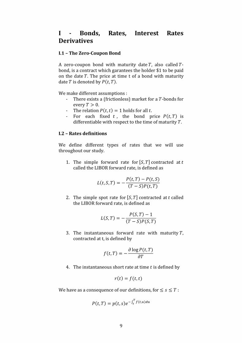
A zero-coupon bond with maturity date �, also called �-bond, is a contract which garantees the holder $1 to be paid on the date �. The price at time t of a bond with maturity date � is denoted by ��, ��. We make different assumptions :

- There exists a (frictionless) market for a �-bonds for every � > 0.

- The relation ��, �� = 1 holds for all �. - For each fixed � , the bond price ��, �� is

differentiable with respect to the time of maturity �. I.2 – Rates definitions

We define different types of rates that we will use throughout our study.

1. The simple forward rate for ��, � contracted at � called the LIBOR forward rate, is defined as ��, �, �� = − ��, �� − ��, �� − ��, ��

2. The simple spot rate for ��, � contracted at � called

the LIBOR forward rate, is defined as ��, �� = − ��, �� − 1�� − ��, ��

3. The instantaneous forward rate with maturity �,

contracted at t, is defined by ��, �� = − � log ��, ��

4. The instantaneous short rate at time � is defined by

�� = ��, �� We have as a consequence of our definitions, for ≤ � ≤ � : ��, �� = ��, �� ,�� !

10

A non-arbitrage argument implies also that ��, �� = " #�� $!�% & 'ℱ�)

We define *�� to be the value of a bank account at time � ≥ 0. We assume *�0� = 1 and that the bank account evolves according to the following differential equation : ,*�� = ��*��,�, *�0� = 1 where �� is a function of time. Hence we can write : *�� = �� $�%��%&- �� is known as the short rate. If we invest $. at time 0, we

have on our our money-market account $.�� $�%��%&- . The bank account grows at each time � at the rate ��. Our purpose is to model this short interest rate with a model which can replicate the one we see on the market. We will look at other rates, financial products build on these rates which are traded every day on financial markets. Based on their prices, we will calibrate our model and see how well they fit the market. I.3 – Interest rates derivatives

I.3.a – Swaps

An interest rate swap is a contract in which two parties agree to exchange interest rate cash flows, based on a specified notional amount from a fixed rate, known as the swap rate to a floating rate, typically a LIBOR rate (or vice versa). We denote the notional by /, and the swap rate by 0. The LIBOR rate fixes on dates �1, �2, … , �4�2. If you swap a fixed rate for a floating rate (LIBOR), then at time �5 you will receive /. ��5 − �5�2�. ��5�2, �5� and you will pay the amount /. ��5 − �5�2�. 0 Hence the net cashflow 75 at time �5 is 75 = /. ��5 − �5�2�. ��5�2, �5� − 0�

11

We call this type of swap an arrear settled payer swap: you pay the fixed rate in exchange of the LIBOR rate, one period after the fixing occurred. By definition of the LIBOR rate, we have: 75 = /. ��5 − �5�2�. 8 1 − ��5�2, �5��5 − �5�2�. ��5�2, �5� − 09

75 = /. ; 1��5�2, �5� − <1 + 0. ��5 − �5�2�>? To compute the value of this specific cashflow at time �, we need to know the price of an asset at time t which value is

equal to 75 at time �5. Selling at time � /. <1 + 0. ��5 − �5�2�>

bonds delivering 1 at time T_i would gives us a net cashflow

of −<1 + 0. ��5 − �5�2�>.

We now need to find how to replicate @A�BCDE,BC�. If we buy at

time �5�2 $N worth of bonds delivering $1 at time �5, which

is to say @A�BCDE,BC�, we get $

@A�BCDE,BC� at time T_i. The value at

time � of / is ��, �5�2�. Hence we have: F�75 , �� = /. G��, �5�2� − ��, �5�<1 + 0. ��5 − �5�2�>H

And the price of a payer swap is hence equal to: IJKLI��, 0, �1, �4�

= / M G��, �5�2�45N2− ��, �5�<1 + 0. ��5 − �5�2�>H

Usually, when two parties enter a swap, they agree to have a fixed rate 0∗ such that the price of the swap is equal to zero when the swap starts. Hence we have: 0∗ = ∑ ��, �5�2� − ��, �5��45N2∑ ��5 − �5�2��, �5�45N2

0∗ = ��, �1� − ��, �4�∑ ��5 − �5�2��, �5�45N2

12

We call 0∗ the swap rate. One of the main interests of swaps is to exchange floating, and then risky cashflows, against a fixed, and hence risk-free cashflows. For example, a company who wants to secure a loan can use it. But it presents also some disadvantages: if the floating rate is lower than the fixed rate, the company who pays (the fixed leg) loses money. Hence there is another way to hedge these floating cashflow, without losing money when the fixed rate is higher than the floating rate. I.3.b – Caps, Floors

Following our last example, there exist contracts that allow us to receive, when the fixed rate is higher than the floating rate, the difference of these two rates multiplied by a specific notional. Caps are contracts having these specifications. A cap with cap rate R and resettlement dates �1, … , �4 is a contract which at time � 52Q5Q4 gives the holder of the cap the

amount : R5 = ��5 − �5�2� max��5�2, �5� − 0, 0 We also define a floor, with cap rate R and resettlement dates �1, … , �4 , which is a contract which at time � 52Q5Q4 that

gives the holder of the floor the amount : V5 = ��5 − �5�2� max��5�2, �5� − 0, 0 When W = 1 (i.e. there is only one payment), we use the term caplet and floorlet. Caps and floors can then be reduced to streams of caplets and floorlets. When we will have to compute the prices of caps and floors, we will only need to know how to compute the prices of caplets and floorlets. I.3.c – Swaptions

Another famous interest rate derivative is the swaption. Such a product gives the right to its owner to enter in a payer swap (we call the it a payer swaption) or a receiver swap (receiver swaption). Let us note that a payer swaption and a cap covering the same string of cashflows would have

13

different prices. When we decide to exercise such a swaption (the swap rate on the market is higher than the swap rate – or strike - embedded in the swaption), we enter a swap and have to exchange flows until the maturity of the swap, even if we sart loosing money when exchanging the flows. A caps only pays positive cashflows ; in fact we can see it as the right to decide wether or not we exchange flows on a payment date. Since there is more optionality in a cap than in a swaption covering the same period, the cap would be more expensive. We will focus on European Swaptions, which are swaptions which can be exercised one time only (there also exists American Swaptions, which can be exercised anytime, and more commonly Bermudan swaptions, which can be exercised periodicaly). Let us consider a payer swaption with strike X and exercise date �, which allow us to enter a payer swap with fixing dates � = �1, �2, �Y, … , �4�2 , cashflows occuring on �2, �Y, … , �4 , swap rate X , and notional /. At time � the price of our swap would be ��Z[��, 0, �1, �4�

= / M G��, �5�2�45N2− ��, �5�<1 + X. ��5 − �5�2�>H

And the swap rate 0∗ defined earlier would be 0∗ = 1 − ��, �4�∑ ��5 − �5�2��, �5�45N2

The swaption will obviously not be exercised if X is higher than the swap rate 0∗: it would be less expensive to enter a swap with a fixed rate equal to the swap rate. Hence we see that we must have 0∗ > X to exercise the swaption. Hence we can write its payoff at time � as

max ;/ M G��, �5�2� − ��, �5�<1 + X. ��5 − �5�2�>H45N2 , 0?

which can be rewritten as thanks to the definition of 0∗ :

14

/ max ;M G��, �5�2� − ��, �5�<1 + X. ��5 − �5�2�>H45N2 − M G��, �5�2�4

5N2− ��, �5�<1 + 0∗ . ��5 − �5�2�>H , 0?

and

/ max \�0∗ − X� M ��, �5��5 − �5�2�45N2 , 0]

I.4 – Structured Products

We gives here a rapid overview of the different structured products banks market and sells to corporate clients. These products drives the prices and dynamics of the derivative market. I.4.a – Callable Swaps

If a corporate client wants to enter a payer swap, but wants to pay a lower fixed rate than the swap rate on the market, a bank can offer him to buy another product from him, and the cost of this product will be embedded into the fixed rate. From the customer point of view, the swap will have a positive value, which matches the price of the product he sold to the bank. Typically, a bank will accept to receive a lower fixed rate if it gets some optionality over the trade. For instance, it can buy from the corporate client a payer swaption, starting in a few years, with a strike equal to the fixed rate of the swap they ae going to enter. The swaption is typically European, and most of the time Bermudan. This product gives the bank the right to enter the opposite swap after a few years. Hence, it allows the bank to “call” the swap at exercise time(s), which is equivalent to cancel it. Hence a callable payer swap allows a customer to pay less to have access to the floating rate (usually LIBOR). One of the downside is that he takes the risk to see the swap terminated sooner than a regular one.

15

I.4.b – Deposits and Loans

When a corporate client has an excess of treasury and won’t need it until a certain period of time, it can make a simple deposit to the bank. Then bank receives $1M to the customer and pays him the LIBOR rate plus a spread. To make the spread bigger, the client can still sell a product to the client. In this case the product to be sold to the bank would be a cap on LIBOR, which price would be embedded in the spread the bank add to LIBOR. The corporate client would hence receive bigger interests on his deposit, but if LIBOR tends to be bigger than the cap’s strike, the bank would only pay him interest based on the strike level and not LIBOR. The client can also buy a floor from the bank, which would make the spread lower, but would protect him from to low LIBOR rates. I.4.c – Extendable Swaps

A corporate client could also need to enter a receiving swap. Imagine that a client wants to enter a 3 years receiving swap, and also thinks that the rates will increase in 3 years. He could enter a 3 year swap with the bank and sell it a receiver swaption expiring in 3 years, offering the bank the opportunity to enter a payer swap at the same fixed rate than the one it enters today against the client. To match the price of the swaption, the fixed rate received by the client from the bank would be higher. If the client’s view of rates increasing in 3 years were correct, then the bank would not exercise the payer swaption., and he would have receive a higher rate than the 3 year swap rate. In exchange, it offers the banks the possibility to extend the swap for another two years if rates would stay low. This kind of product might especially be popular when rates are low, with a lot of uncertainty on the future, giving the options (which basically are insurance against the future) more value. I.5 – Discounting and Credit Risk

We see that to discount cashflows with respect to time , we multiply them by bond prices (which we also call discount factors). This is due to the no-arbitrage assumption. In reality, this is not true : markets do a distiction betwen the rates on which the option is, and the rates which will be

16

used to discount the cashflows. To make the the thesis readible, we will consider that this is not the case here. But here are some reasons about the differences. The discount curve might vary with respect to products : for example, GBP european swaptions are discounted on SONIA (« Sterling OverNight Index Average »), but the interests are paid on LIBOR (« London Interbank Offered Rate ») ; on the opposit, GBP bermudean swaptions keeps being discounting on LIBOR. The discount curve might also change as the client change :we can include the risk of credit in the discounting curve, by adding a spread related to his default risk. For example, a top tier bank with good credit rating and a major company with a high default risk would not pay the same price for a similar product. This is commonly taken into the discounting method. Moreover, it is more and more common to use a collaterals to reduce the risk of default between two counterparties. Let us take another example. Bank A sells a swaption expiring in 10 years to Bank B. Bank A will receive £10,000,000 from bank B, and bank B will handle an option which allows him to receive money from bank B in 10 years. Let us suppose Bank A goes bankrupt : it won’t be able to honor the contract in 10 years. Hence the option does not exist anymore and bank B has lost 10 millions. To avoid these problems, bank A can post a collateral : It will make a deposit in bank B of the previous 10 millions, and bank B will pay interest to A on these 10 millions. Hence, if bank A defaults, the swaption dissapears, but bank B has its money back. Bank A can also chose to post a collateral in EUR or in SEK instead of GBP, hence B will have to pay interests with respect to these currencies. The swaption price should be discounted at the rates corresponding to the currency of the collateral ! That is why we see more and more products based on a market but discounted with respect to another market. The discounting model itself is nowadays complicated enough to be a complete subject of another thesis.

17

II – The Hull-White Short Rate Models II.1 – The One-Factor Hull White Model

We assume that our short rate follows the dynamics : ,�� = <^�� − _��>,� + `,Z��

with Z�� a Wiener process, and ^�� a deterministic function of time. This is a more general dynamics than the Vasicek model : ,�� = <^ − _��>,� + `,Z��

with ^ a positive constant. The solution of the equation of the previous SDE is �� = ��a��1 + _ �1 − ��a�� + `��a� b �a�,Z�c��

1

The short rate has a normal distribution, with mean "�� = ��a��1 + _ �1 − ��a��

and variance

d_�<��> = `Y2_ �1 − ��Ya��

we see that when � → ∞, we have

"�� → _

d_�<��> → `Y2_

and the distribution of �� tends to h Gia , jkYaH.

From the expression of "�r�t� and Var<r�t�>, we see that

the bigger the value of a, the « faster » r�t� tends to its limit distribution. We call a the mean reversion : it defines how the short rates dynamics tend to a limit mean. Negatives Rates

Since the Hull-White model implies that the short rate has a normal distribution, this short rate could technically take

18

every value of ℝ, and a fortiori negatives values. In fact, we can even compute the probability of it relatively easily: �� ≤ 0� = � 8pd_�<��>q + "�� ≤ 09

= � rsq ≤ − "��

pd_�<��>tu

with q a random variable such that q~h�0,1�. Hence we have:

�� ≤ 0� = w rs− "��

pd_�<��>tu

What would happen if the short rate were near 0? When rates on the market are very low, volatility tends to be also very low. In the One-Factor Hull-White model, this would be equivalent to have a bigger mean reversion and a smaller \theta(t). From the expression of r(t), we see that the bigger the mean reversion, the lower the variance or r(t). Note: One would think that negative rates would be impossible in real life ; however, we have seen recently that banks trading CHF (Swiss Franc) exchange a negative overnight rate. II.2 - The Two-Factor Hull-White Model

II.2.a – The motivation for multiple factor models

The short rate and its distributional properties suffice to characterize the yield curve, as we have the relation : ��, �� = " xexp − b ��,�B

� {

and the fact that with all the bond prices, we can reconstruct the yield curve. However, a poor short rate model would lead to a poor representation of the yield curve and its evolution. One-

19

factor models such as the classic Hull-White gives 100% correlated LIBOR rates. We see that in reality this is not the case, as we often see the yield curve steepening (short term LIBOR rates get lower, long term LIBOR rates get higher). A one-factor model only allows us to parallel moves of the yield curve. II.2.b – Definition

We have seen that the One-Factor Hull-White model is a model where the rates tends to reach a limit mean given by ^�� at a certain pace, given by the mean reversion _. The function ^�� is deterministic, but an intuitive way would be to add it a stochastic component c��, in fact to give it the structure of the One-Factor Hull-White model, with a mean reversion |, lower than _. Hence, after a certain time, our short rate model would tend to a one-factor stochastic function which would then itself tend to a deterministic function. We would then introduce a correlation factor } between the Wiener processes driving the dynamics of �� and c��. This leads us to study the Two-Factor Hull-White model : ,�� = <^�� + c�� − _~��>,� + 2��,Z2�� ,c�� = −|~c��,� + Y��,ZY�� with ,Z2��,ZY�� = },�. II.3 – Equivalence to the Two-Additive-Factor Gaussian

Model

The two factor Hull-White model is defined such that it assumes the short rate evolves in the risk-adjusted measure according to : ,�� = <^�� + c�� − _~��>,� + 2,q2��, ��0� = �1 ,c�� = −|~c��,� + Y,qY��, c�0� = 0 with �q2, qY� a two dimensional Brownian motion such that ,q2��,qY�� = },� , �1, _~, |~, 2, Y positive constants, and −1 ≤ } ≤ 1. The deterministic function ^�� is chosen to fit the current term structure of interest rates. We define the the new stochastic process �� = �� + �c��

20

where � = 2�~�a~. By differentiating ��, we get :

,�� = <^�� + c�� − _~��>,� + 2,q2�� − �|~c��,�+ � Y,qY�� ,�� = G^�� + c�� − _~�� − �|~c��H ,� + 2,q2��+ � Y,qY�� ,�� = �^�� − _~��,� + �,q�� with :

� = � 2Y + YY<_~ − |~>Y + 2} 2 Y|~ − _~ ,q�� = 2,q2�� − Y_~ − |~ ,qY��

�

Moreover, we define another new stochastic process : �� = −�c�� = c��_~ − |~

The differentiation of �� gives us : ,�� = − |~_~ − |~ c��,� + Y_~ − |~ ,qY�� ,�� = −|~��,� + �,qY�� with :

� = Y_~ − |~

Hence we can write �� = �� + �� + �� where ,�� = −_~��,� + �,q�� ,�� = −|~��,� + �,qY�� = �1��a~� + b ^��a~��,��

1 Hence we see that the Hull-White Two-Factor Model is equivalent to a « Two-Additive-Factor Gaussian Model ». This equivalence is going to be very useful to us. If it is more easy to interpret the different parameters of the Hull-White

21

model and their influence on the price and volatility structures, the shape of the Gaussian model allows us to easier calculations for the prices of bonds and derivatives. We have a perfect equivalence between the two models. If we write the HW2F as follow : ,�� = <^�� + c�� − _~��>,� + 2,q2��, ��0� = �1 ,c�� = −|~c��,� + Y,qY��, c�0� = 0 such that ^�� is a deterministic function of time and ,q2��,qY�� = } And the G2++ as follow : �� = .�� + �� + �� ,.�� = −_.��,� + `,Z2�� ,�� = −|��,� + �,ZY�� with �� a deterministic function of time such that ��0� = �1, then we the coresponding equivalences between each parameters of the two models : _ = _~ | = |~

` = � 2Y + YY<_~ − |~>Y + 2} 2 Y|~ − _~ � = Y_~ − |~ } = 2} − �` �� = �1��a~� + b ^��a~��,��

1

or, put in the other way : _~ = _ |~ = |

2 = �`Y + �Y + 2}`� Y = ��_ − |� } = `} + �2

^�� = ,��,� + _��

We will now proceed as follow : 1) We will calculate and calibrate everything in the G2++ framework, and then 2)

22

analyze the equivalent parameters of the Two-Factor Hull-White model.

23

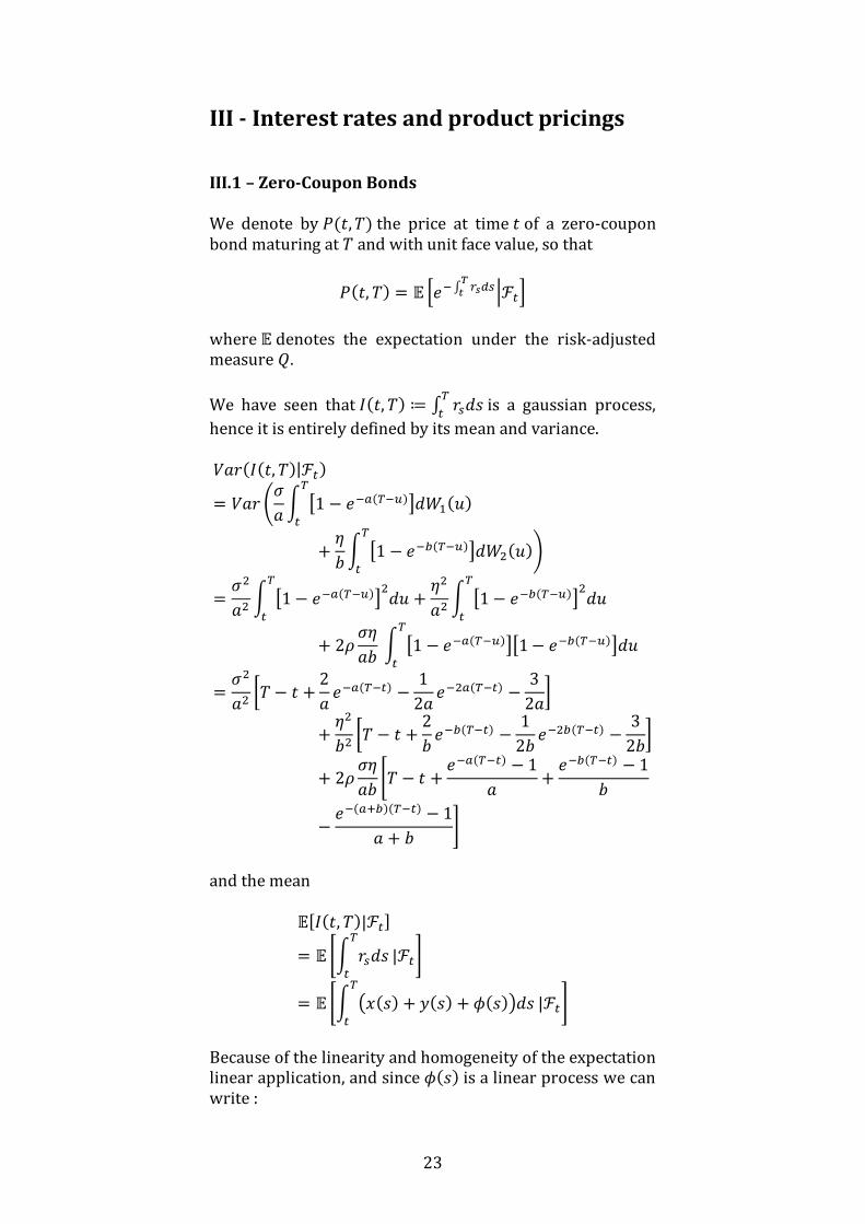
III - Interest rates and product pricings III.1 – Zero-Coupon Bonds

We denote by ��, �� the price at time � of a zero-coupon bond maturing at � and with unit face value, so that ��, �� = " #�� $!�% & 'ℱ�)

where " denotes the expectation under the risk-adjusted measure �.

We have seen that ��, �� ≔ � �%,�B� is a gaussian process,

hence it is entirely defined by its mean and variance. d_��, ��|ℱ�� = d_� 8_ b �1 − ��a�B��,Z2�c�B

� + �| b �1 − ��B��,ZY�c�B� 9

= `Y_Y b �1 − ��a�B��Y,cB� + �Y_Y b �1 − ��B��Y,cB

�+ 2} `�_| b �1 − ��a�B��1 − ��B��,cB�

= `Y_Y �� − � + 2_ ��a�B�� − 12_ ��Ya�B�� − 32_�+ �Y|Y �� − � + 2| ��B�� − 12| ��Y��B�� − 32|�+ 2} `�_| x� − � + ��a�B�� − 1_ + ��B�� − 1|− ��a��B�� − 1_ + | {

and the mean "��, ��|ℱ� = " xb �%,�B

� |ℱ�{ = " xb <.�� + �� + ��>,�B

� |ℱ�{

Because of the linearity and homogeneity of the expectation linear application, and since �� is a linear process we can write :

24

"��, ��|ℱ� = b "�.��|ℱ� ,�B� + b "��|ℱ� ,�B

�+ b ��,�B�

Hence by the definition of x, y and �, the calculation is pretty straightforward, and gives : "��, ��|ℱ� = 1 − ��a�B��_ .�� + 1 − ��B��| ��

+ b ��,�B�

We know that if q is a normal random variable with mean �� and variance `Y , then "�exp�q� = exp G�� + 2Y �YH . −��, �� is a normal random variable whose mean and variance are now known. Hence ��, �� = ��2��D�� D&�a ��2��D�� D&�� %��% & �2Y¡��,B� In particular, we have ��0, �� = �� %��% - �2Y¡�1,B� This expression must fit the actual market, which means that for each � ≤ � ∗ we must have : �¢�0, �� = �� %��% - �2Y¡�1,B� Which leads us to �� %��% - = �¢�0, ��2Y¡�1,B� and for � ≤ � ≤ � ∗

�� %��% & = �� %��% - �� %��%&- = �� %��% &�� %��%&-= �¢�0, ��¢�0, �� 2Y<¡�1,B��¡�1,��>

We can now rewrite the price of the zero coupon bond, fitting the current market, with our Hull-White parameters :

25

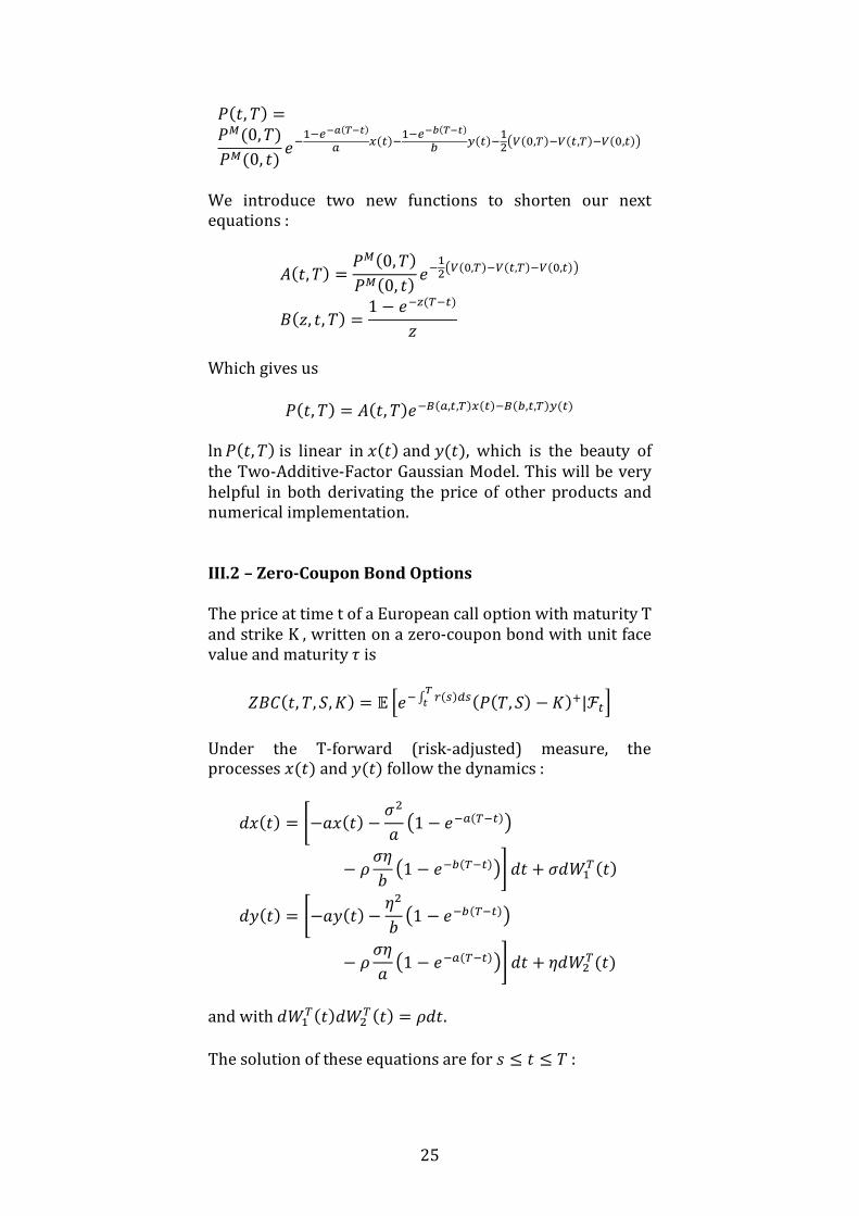
��, �� = �¢�0, ��¢�0, �� 2��D�� D&�a ��2��D�� D&�� 2Y<¡�1,B��¡��,B��¡�1,��>

We introduce two new functions to shorten our next equations : [��, �� = �¢�0, ��¢�0, �� 2Y<¡�1,B��¡��,B��¡�1,��>

*�£, �, �� = 1 − ��B��£

Which gives us ��, �� = [��, ��¤�a,�,B��¤��,�,B�� ln ��, �� is linear in .�� and ��, which is the beauty of the Two-Additive-Factor Gaussian Model. This will be very helpful in both derivating the price of other products and numerical implementation. III.2 – Zero-Coupon Bond Options

The price at time t of a European call option with maturity T and strike K , written on a zero-coupon bond with unit face value and maturity ¦ is q*§��, �, �, X� = " #�� $�%��% & ��, �� − X��|ℱ�)

Under the T-forward (risk-adjusted) measure, the processes .�� and �� follow the dynamics : ,.�� = x−_.�� − `Y_ <1 − ��a�B��>

− } `�| <1 − ��B��>{ ,� + `,Z2B�� ,�� = x−_�� − �Y| <1 − ��B��>

− } `�_ <1 − ��a�B��>{ ,� + �,ZYB�� and with ,Z2B��,ZYB�� = },�.

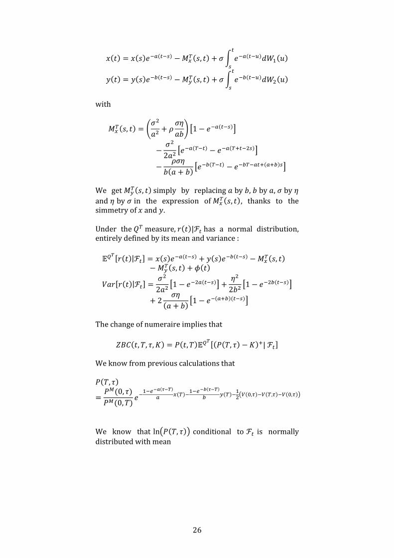
The solution of these equations are for � ≤ � ≤ � :

26

.�� = .��a��%� − ¨�B��, �� + ` b ��a��,Z2�c��%

�� = ��%� − ¨�B��, �� + ` b ��,ZY�c��%

with ¨�B��, �� = 8`Y_Y + } `�_|9 �1 − ��a��%��

− `Y2_Y ��a�B�� − ��a�B��Y%��− }`�|�_ + |� ��B�� − ��B�a��a��%�

We get ¨�B��, �� simply by replacing _ by |, | by _, ` by �

and � by ` in the expression of ¨�B��, ��, thanks to the simmetry of . and �. Under the �B measure, ��|ℱ� has a normal distribution, entirely defined by its mean and variance : "© ��|ℱ� = .��a��%� + ��%� − ¨�B��, ��− ¨�B��, �� + �� d_��|ℱ� = `Y2_Y �1 − ��Ya��%�� + �Y2|Y �1 − ��Y��%��+ 2 `��_ + |� �1 − ��a��%��

The change of numeraire implies that q*§��, �, ¦, X� = ��, ��"© ��, ¦� − X��| ℱ� We know from previous calculations that ��, ¦�= �¢�0, ¦��¢�0, �� 2��D��ªD �a ��B��2��D��ªD �� B��2Y<¡�1,«��¡�B,«��¡�1,«�>

We know that ln<��, ¦�> conditional to ℱ� is normally

distributed with mean

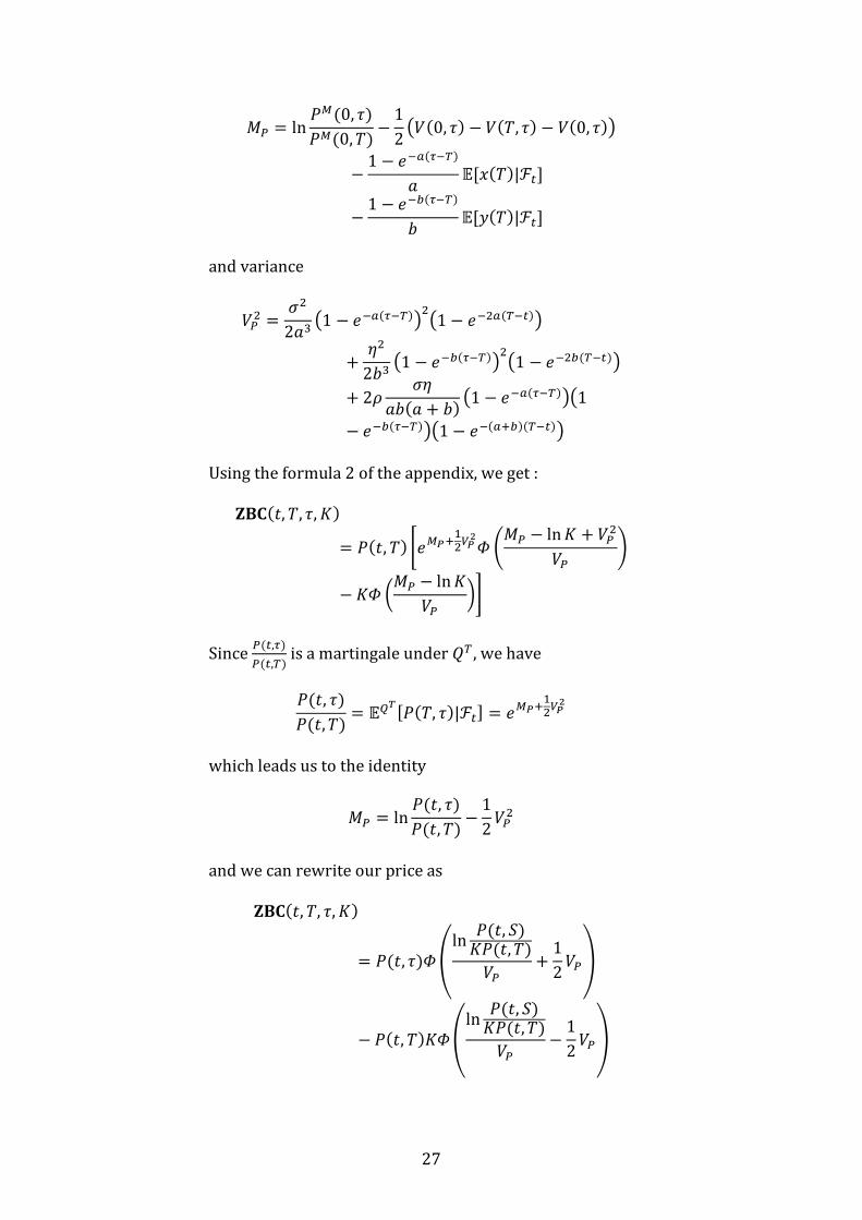
27

Ä = ln �¢�0, ¦��¢�0, �� − 12 <d�0, ¦� − d��, ¦� − d�0, ¦�>− 1 − ��a�«�B�_ "�.��|ℱ� − 1 − ��«�B�| "��|ℱ�

and variance dAY = `Y2_� <1 − ��a�«�B�>Y<1 − ��Ya�B��>

+ �Y2|� <1 − ��«�B�>Y<1 − ��Y��B��>+ 2} `�_|�_ + |� <1 − ��a�«�B�><1− ��«�B�><1 − ��a��B��>

Using the formula 2 of the appendix, we get : ¬®��, �, ¦, X�= ��, �� x�¢¯�2Y¡kw 8Ä − ln X + dAYdA 9

− Xw °Ä − ln XdA ±{

Since A��,«�A��,B� is a martingale under �B , we have

��, ¦��, �� = "© ��, ¦�|ℱ� = �¢¯�2Y¡k

which leads us to the identity Ä = ln ��, ¦��, �� − 12 dAY

and we can rewrite our price as ¬®��, �, ¦, X�

= ��, ¦�w ²ln ��, ��X��, ��dA + 12 dA³− ��, ��Xw ²ln ��, ��X��, ��dA − 12 dA³

28

III.3 – Caps and Floors

We have seen that a cap/floor is a thread of simple options on LIBOR forward rates known as caplets and floorlets. We show that a caplet (or a floorlet) is actually equivalent to a put (or a call) option on a bond. The price of a caplet a time 0, with notional N and strike K which fixes at time �2 and pays at time �Y is given by : ®´µ��, �2, �Y, /, R�= " #�� $!�% k& /��Y − �2��2, �Y� − R��'ℱ�)

where ��2, �Y� is the LIBOR rate, defined by : ��, �� = 1 − ��, �� − ��, ��

We can thus rewrite the caplet price as : ®´µ��, �2, �Y, /, R�= " x�� $!�% k& /��Y − �2� 8 1 − ��2, �Y��Y − �2��2, �Y� − R9� ¶ℱ�{ ®´µ��, �2, �Y, /, R�= /" ·�� $!�% E& ��2, �Y� ;1 − ��2, �Y��2, �Y� − R��Y − �2�?� ¸ℱ�¹ ®´µ��, �2, �Y, /, R�= /" �� $!�% E& G1 − <1 + R��Y − �2�>��2, �Y�H� ºℱ�� ®´µ��, �2, �Y, /, R� = /′" #�� $!�% E& <X − ��2, �Y�>�'ℱ�)

with /¼ = /<1 + R��Y − �2�> X = 1<1 + R��Y − �2�>

We notice that the structure of the price of a caplet is identical to a bond put’s with strike K and notional N’. By the same reasonning, we can show that a floorlet is equivalent to a call on a bond. If we know the arbitrage free price of an european option on a bond, we will deduce from it the prices of caplets/floorlets, and by extension, the price of caps/floors.

29

III.4 – Swaptions

The arbitrage free price at time � = 0 of a european arrear settled payer swaption is given by numerically computing the following one-dimensional integral : IJK½I¾ �0, �, ¿, /, R, À� =

/À��0, �� b ��2YG��ÁÂjÂ Hk�√2Ä ·w<−Àℎ2�.�>�∞

�∞− M Æ5�.��ÇC��w<−ÀℎY�.�> 4

5N2 ¹ ,.

where À = 1 (À = −1) for a payer (receiver) swaption, ℎ2�.� ≔ �~ − È�`��1 − }��Y − }��. − È��

��1 − }��Y ℎY�.� ≔ ℎ2�.� + *�|, �, �5�`�p1 − }��Y Æ5�.� ≔ 75[��, �5��¤�a,B,�C�� É5�.� = −*�|, �, �5� xÈ� − 12 <1 − }��Y >`�Y*�|, �, �5�

+ }��`��. − È�� {

�~ ≔ �~�.� is the unique solution of the following equation

M 75[��, �5��¤�a,B,�C��¤��,B,�C��~45N2 = 1

and È� ≔ −¨�B�0, �� È� ≔ −¨�B�0, ��

� ≔ `�1 − ��YaB2_ `� ≔ `�1 − ��Y�B2| }�� ≔ }`��_ + |� �`� �1 − ��a��B�

We derive this expression by taking the arbitrage free price of the european swaption:

30

Ê��0, �, ¿, /, R, À� = /��0, ��"B Ë·À ;1 − M 75��, �5�4

5N2 ?¹�Ì = /��0, �� b ·À ;1ℝk− M 75[��, �5��¤�a,B,�C��¤��,B,�C��4

5N2 ?¹� ��., ��,�,.

where f is the random vector <.��, ��>, i.e.,

��., ��≔ exp ;− 12<1 − }��Y > 8G. − È�� HY − 2}�� . − È��<� − È�>�`� + °� − È�`� ±Y9?

2Ä �`��1 − }��Y

for each ., we integrate over � from −∞ to ∞ , we get

b ;1 − M Æ5��¤��,B,�C��45N2 ? Í�Î�Ï<��ÁÐ>�Ñ<��ÁÐ>k,�Ò×∞

�~��

with Í ≔ 12Ä �`��1 − }��Y

Ê ≔ − 12<1 − }��Y > °. − È�� ±Y Ô ≔ }��1 − }��Y . − È��`� Õ ≔ 12<1 − }��Y >`�Y

Using integral formulas, our previous expression becomes :

31

Í √Ä√Õ �Î�Ïk�Ñ ËÀ + 12 − w ;<�~ − È�>√2Õ − Ô√2Õ?− M Æ5��¤��,B,�C�ÁÐ�¤��,B,�C��¤��,B,�C��YÏ �Ñ4

5N2∙ \À + 12− w ;<�~ − È�>√2Õ − Ô − *�|, �, �5�√2Õ ?]Ì

Using the identity that for each constant z we have Ò�2Y − Φ�£� = ÀΦ�−À£� and by noting that we have

Í √Ä√Õ = 1�√2Ä

Ê + ÔY4Õ = − 12 °. − È�� ±Y Ô√2Õ = }��1 − }��Y . − È�� √2Õ = 1`��1 − }��Y

We then obtain the expression for the swaption price.

33

IV – Calibration on Caps Prices and

Volatilities I – Purpose and Methodology

To build new interest rates derivatives products to help customers to catch the behaviour of the yield curve and the volatility grids for different period of times, traders want to have a simple feel of the market. Most of the pricing is done with one parameters for each tenor or expiry. For example, there will be a set of parameter for each swaption and each cap traded on the market. Reading through all these set of parameters (which represents several hundreds of numbers) can be difficult and make it uneasy to « feel » the market as a whole. Our purpose here is to use the Two-Factor Hull-White model to modelize the implied volatilies and market prices of a set of caplets. We have access to a number of prices and Black-Scholes implied volatilities for caplets on different markets (Sterling Pound, Euro, Swedish Crown). We don’t have any restrictions on the ressources or time to calibrate our model, so we chose a simple but efficient algorithm. Our methodology is fairly simple : 1) we allow ourself a range of acceptable values for our

data : 0 < |~ < _~ < 200% , 0 < 2,Y < 50% , and 0 ≤ |}| ≤ 1. 2) we use a grid (defined by a step value) to define some key values for each parameters (the smaller the step value, the more key values set we get). 3) we calculate the set of prices caplets for each of the key values sets. 4) we choose the only key values set which produces the best fitting price curve (with a least square method). 5) We invert our model prices with the Black-Scholes formula to get the implied volatility curve by the model. This method could look primitive and not very elaborate, but it produces very good results with a step value small enough. Moreover, we don’t need a live update of the 5 parameters, but only a daily refresh.

34

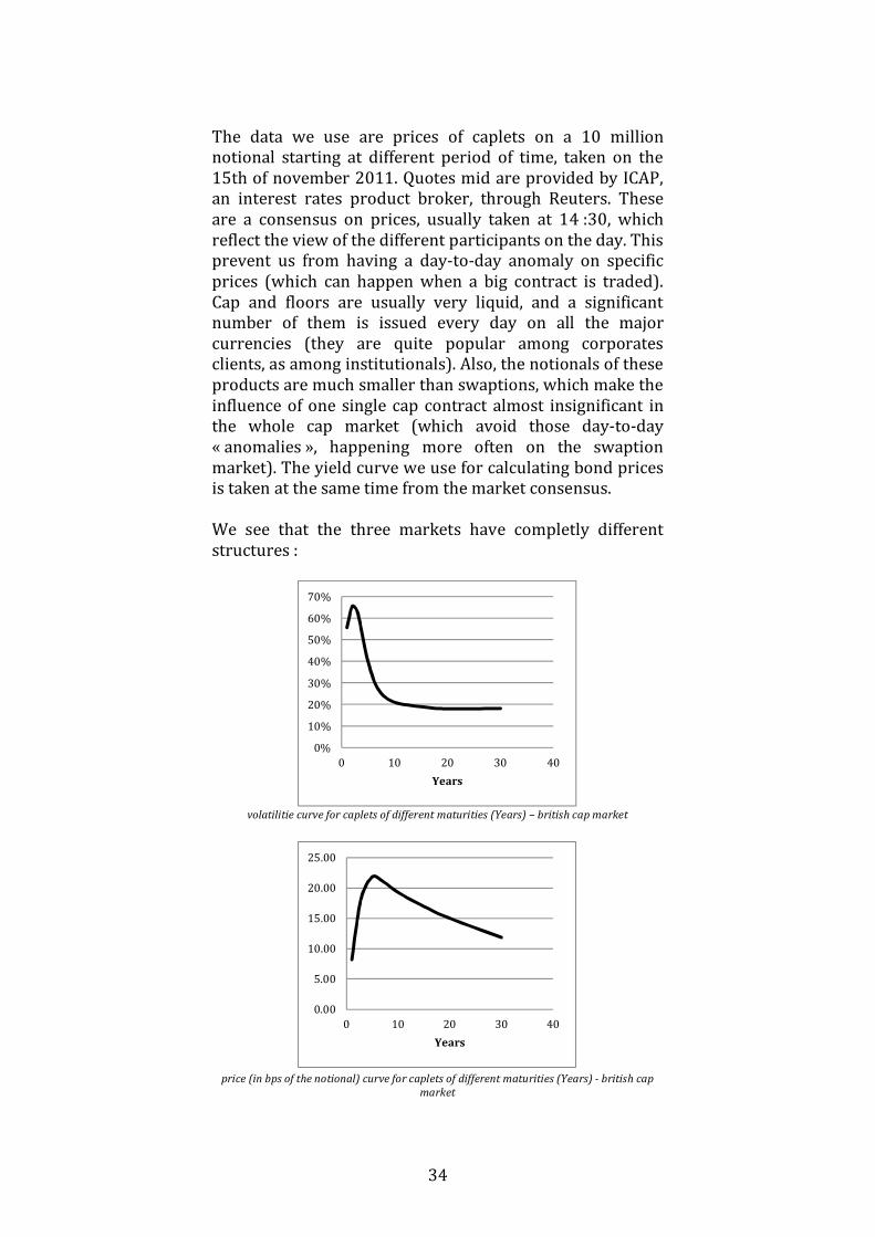
The data we use are prices of caplets on a 10 million notional starting at different period of time, taken on the 15th of november 2011. Quotes mid are provided by ICAP, an interest rates product broker, through Reuters. These are a consensus on prices, usually taken at 14 :30, which reflect the view of the different participants on the day. This prevent us from having a day-to-day anomaly on specific prices (which can happen when a big contract is traded). Cap and floors are usually very liquid, and a significant number of them is issued every day on all the major currencies (they are quite popular among corporates clients, as among institutionals). Also, the notionals of these products are much smaller than swaptions, which make the influence of one single cap contract almost insignificant in the whole cap market (which avoid those day-to-day « anomalies », happening more often on the swaption market). The yield curve we use for calculating bond prices is taken at the same time from the market consensus. We see that the three markets have completly different structures :

volatilitie curve for caplets of different maturities (Years) – british cap market

price (in bps of the notional) curve for caplets of different maturities (Years) - british cap

market

0%

10%

20%

30%

40%

50%

60%

70%

0 10 20 30 40

Years

0.00

5.00

10.00

15.00

20.00

25.00

0 10 20 30 40

Years

35

volatility curve for caplets of different maturities (Years) – swedish cap market

price (in bps of the notional) curve for caplets of different maturities (Years) - swedish cap

market

volatility curve – european cap market

0%

2%

4%

6%

8%

10%

12%

14%

16%

18%

0 10 20 30 40

Years

0

2

4

6

8

10

12

14

0 10 20 30 40

Years

0%

10%

20%

30%

40%

50%

60%

70%

80%

0 10 20 30 40

Years

36

price (in bps of the notional) curve for caplets of different maturities (Years) - european cap

market

The british volatility curve shows a very pronounced hump (more than 60%) on caps starting in 2 and 3 years, and then falls to remain almost constant at 20% after 10 years. One of the reason for such a structure could be that the majority of the caps do not go much higher than 10 years. Hence traders do no quote actively longer caps and hence do not have interest on this part of the volatility curve, which remains constant by convenience. The swedish market follows a similar behaviour, although the volatility remain quite stable (between 16% and 10%). The European volatility curve show an « atypical » hump around 20 years, which could show that traders are uncertain on the long term forward rates, which increase the price of options on these part of the yield curve. IV.2 - Analysing the Results

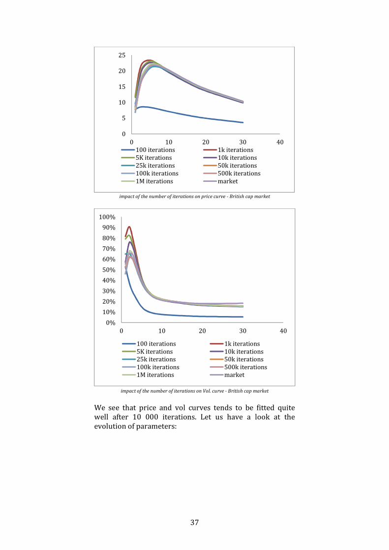
IV.2.a - Impact of the number of iterations

We ran our calibration for different numbers of iterations on the british market to see how our estimated parameters and volatilities evolves as the number of iterations increases. We noticed that after 1 000 000 iterations (which takes 5 minutes calculation time) our resuts appears to be satisfying enough. Here are the different prices and volatility curves:

0

5

10

15

20

25

0 10 20 30 40

Years

37

impact of the number of iterations on price curve - British cap market

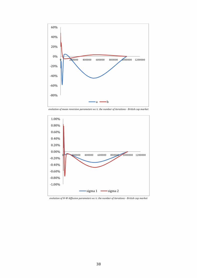
impact of the number of iterations on Vol. curve - British cap market We see that price and vol curves tends to be fitted quite well after 10 000 iterations. Let us have a look at the evolution of parameters:

0

5

10

15

20

25

0 10 20 30 40100 iterations 1k iterations5K iterations 10k iterations25k iterations 50k iterations100k iterations 500k iterations1M iterations market

0%

10%

20%

30%

40%

50%

60%

70%

80%

90%

100%

0 10 20 30 40

100 iterations 1k iterations5K iterations 10k iterations25k iterations 50k iterations100k iterations 500k iterations1M iterations market

38

evolution of mean reversion parameters w.r.t. the number of iterations - British cap market

evolution of H-W diffusion parameters w.r.t. the number of iterations - British cap market

-80%

-60%

-40%

-20%

0%

20%

40%

60%

0 200000 400000 600000 800000 1000000 1200000

a b

-1.00%

-0.80%

-0.60%

-0.40%

-0.20%

0.00%

0.20%

0.40%

0.60%

0.80%

1.00%

0 200000 400000 600000 800000 1000000 1200000

sigma 1 sigma 2

39

evolution of H-W correlation parameter w.r.t. the number of iterations - British cap market

IV.2.b - Fitting different markets : GBP, SEK, EUR

We ran our calibrations for the three market with one million iterations for each. Here are ou results, with our Hull-White parameters (calculated from the Two-Factor Gaussian model) and plots of both volatility and price curves. The british market: _~ = 96,92% |~ = 24,04% 2 = 0,47% Y = 1,18% } = −78,79%

volatility curve: Market vs. Two-Factor Hull-White model – British market

-60%

-40%

-20%

0%

20%

40%

60%

80%

100%

120%

140%

160%

0 200000 400000 600000 800000 1000000 1200000

correlation

0.00%

10.00%

20.00%

30.00%

40.00%

50.00%

60.00%

70.00%

80.00%

0 10 20 30 40

HW2F model market levels

40

price curve: Market vs. Two-Factor Hull-White model – British market

The swedish market: _~ = 90,47% |~ = 11,58% 2 = 0,91% Y = 0,90% } = −97,24%

volatility curve: market vs. Two-Factor Hull-White model – Swedish market

price curve: Market vs. Two-Factor Hull-White model – Swedish market

0.00

5.00

10.00

15.00

20.00

25.00

0 10 20 30 40


0.00%

2.00%

4.00%

6.00%

8.00%

10.00%

12.00%

14.00%

16.00%

18.00%

0 10 20 30 40


0.00

2.00

4.00

6.00

8.00

10.00

12.00

14.00

0 5 10 15 20 25 30 35


41

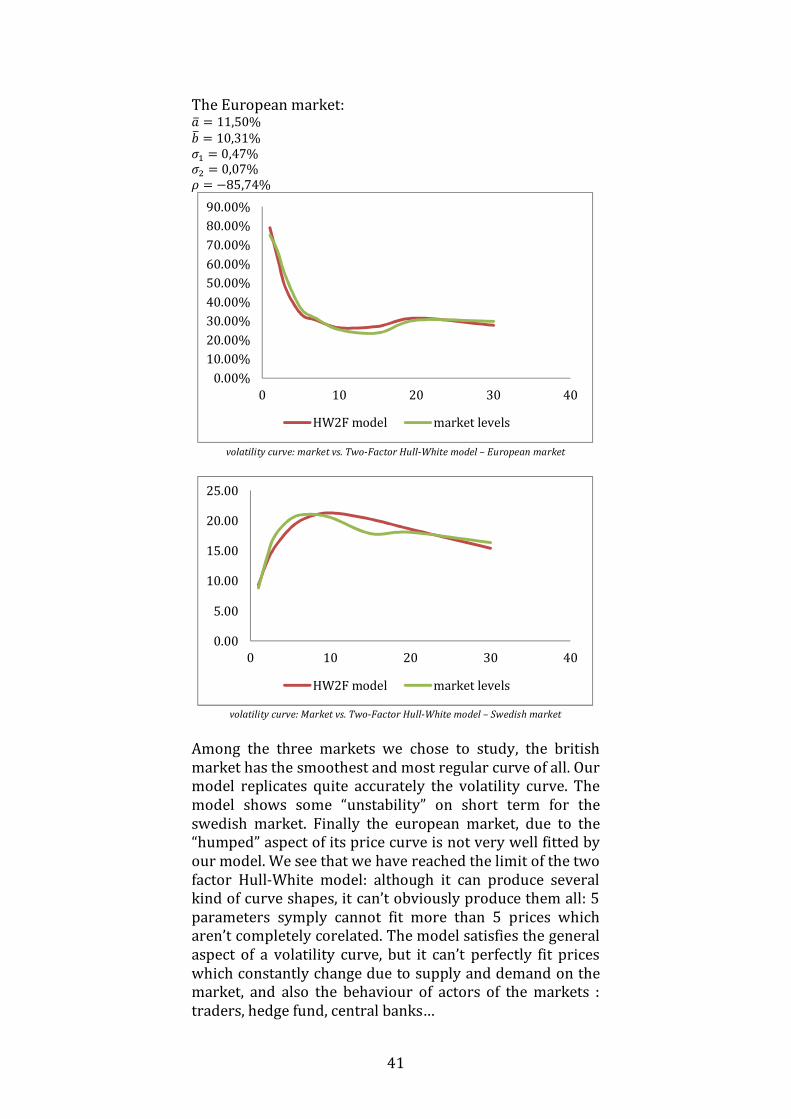
The European market: _~ = 11,50% |~ = 10,31% 2 = 0,47% Y = 0,07% } = −85,74%

volatility curve: market vs. Two-Factor Hull-White model – European market

volatility curve: Market vs. Two-Factor Hull-White model – Swedish market

Among the three markets we chose to study, the british market has the smoothest and most regular curve of all. Our model replicates quite accurately the volatility curve. The model shows some “unstability” on short term for the swedish market. Finally the european market, due to the “humped” aspect of its price curve is not very well fitted by our model. We see that we have reached the limit of the two factor Hull-White model: although it can produce several kind of curve shapes, it can’t obviously produce them all: 5 parameters symply cannot fit more than 5 prices which aren’t completely corelated. The model satisfies the general aspect of a volatility curve, but it can’t perfectly fit prices which constantly change due to supply and demand on the market, and also the behaviour of actors of the markets : traders, hedge fund, central banks…

0.00%

10.00%

20.00%

30.00%

40.00%

50.00%

60.00%

70.00%

80.00%

90.00%

0 10 20 30 40


0.00

5.00

10.00

15.00

20.00

25.00

0 10 20 30 40


42

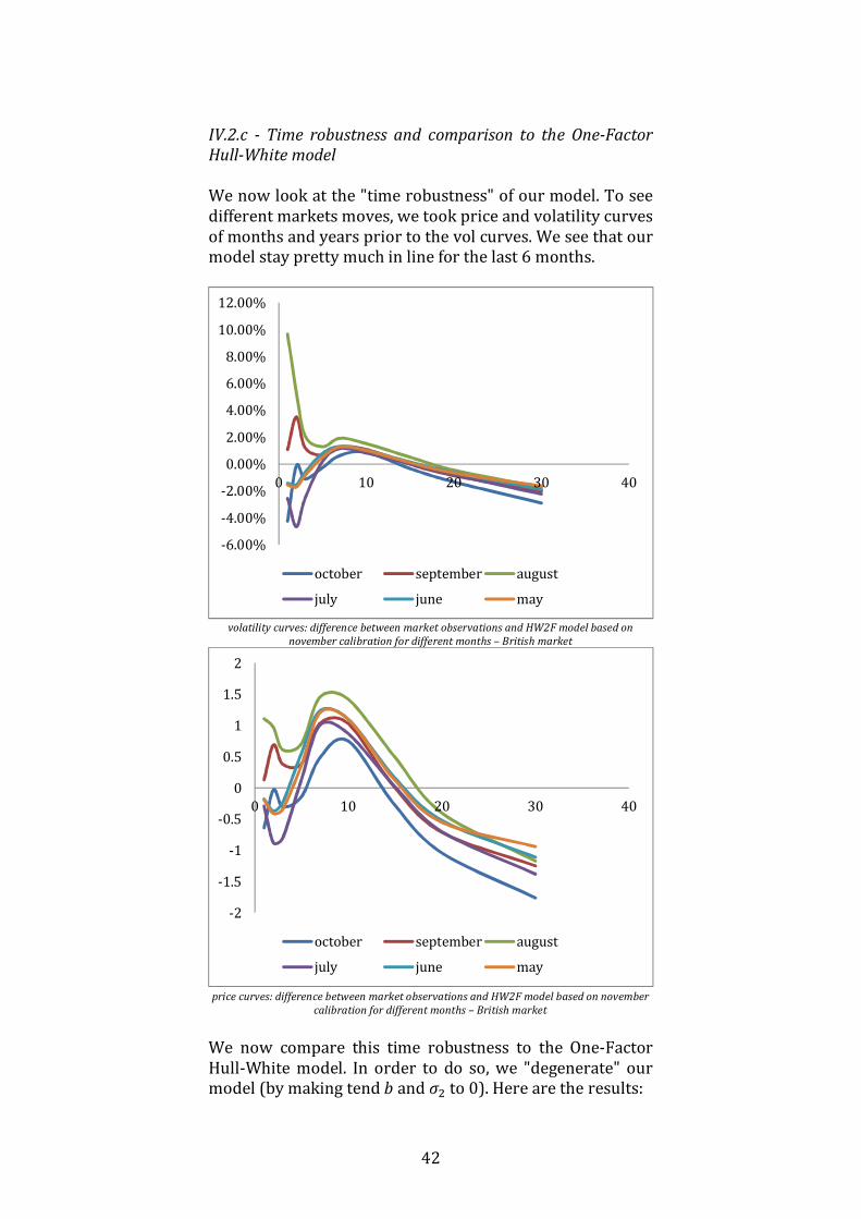
IV.2.c - Time robustness and comparison to the One-Factor

Hull-White model

We now look at the "time robustness" of our model. To see different markets moves, we took price and volatility curves of months and years prior to the vol curves. We see that our model stay pretty much in line for the last 6 months.

volatility curves: difference between market observations and HW2F model based on

november calibration for different months – British market

price curves: difference between market observations and HW2F model based on november

calibration for different months – British market

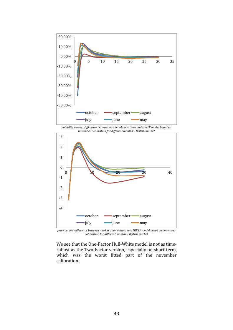
We now compare this time robustness to the One-Factor Hull-White model. In order to do so, we "degenerate" our model (by making tend | and Y to 0). Here are the results:

-6.00%

-4.00%

-2.00%

0.00%

2.00%

4.00%

6.00%

8.00%

10.00%

12.00%

0 10 20 30 40

october september august

july june may

-2

-1.5

-1

-0.5

0

0.5

1

1.5

2

0 10 20 30 40


july june may

43

volatility curves: difference between market observations and HW1F model based on

november calibration for different months – British market

price curves: difference between market observations and HW2F model based on november

calibration for different months – British market

We see that the One-Factor Hull-White model is not as time-robust as the Two-Factor version, especially on short-term, which was the worst fitted part of the november calibration.

-50.00%

-40.00%

-30.00%

-20.00%

-10.00%

0.00%

10.00%

20.00%

0 5 10 15 20 25 30 35


july june may

-4

-3

-2

-1

0

1

2

3

0 10 20 30 40


july june may

45

Conclusion Here is what we achieved with a two factor model. One question one could ask is: what number of factor should we use to have a fit good enough ? It is obvious that the more we add, the more “precise” we will get in our replication of the price and volatility curve at one certain point of time. But we have to compose between the result we want to get and the complexity of how to get them. Historical analysis of the whole yield curve, based on principal component analysis or factor analysis suggests that one component explain 68% to 76% of variations in the yield curve (see Jamshidian and Zhu 1997), two component explain 85% to 90%, and three components 93% to 94%. At its best, a two factor model explain 14% more than a one factor model, and only 4% less than a three factor model. These 4% can hence easily be exchanged against much simpler and more elegant calculations.

47

Bibliography

John Hull and Alan White, "Pricing interest-rate derivative

securities", The Review of Financial Studies, Vol 3, No. 4 (1990) pp. 573–592 John Hull and Alan White, "One factor interest rate models

and the valuation of interest rate derivative securities," Journal of Financial and Quantitative Analysis, Vol 28, No 2, (June 1993) pp 235–254 John Hull and Alan White, "The pricing of options on interest

rate caps and floors using the Hull–White model" in Advanced Strategies in Financial Risk Management, Chapter 4, pp 59–67. Jamshidian and Zhu, LIBOR and swap market models and

measures, in Finance and Stochastics 4 (1997) Thomas Björk, Arbitrage Theory in Continuous Time, Oxford Finance Brigo & Mercurio, Interest Rates Models: Theory and

Practice with Smile, Inflation and Credit, Springer

the two-factor hull-white model : pricing and calibration of

Documents