the twente lower extremity model - xsens
TRANSCRIPT
The Twente Lower Extremity Model
Consistent Dynamic Simulation of the
Human Locomotor Apparatus
Martijn D. Klein Horsman

De promotiecommissie is als volgt samengesteld: Voorzitter en Secretaris: Prof. dr. F. Eising Universiteit Twente Promotoren: Prof. dr. F.C.T. van der Helm Universiteit Twente Prof. dr. ir. H.F.J.M. Koopman Universiteit Twente Leden: Prof. dr. ir. J. Rasmussen Aalborg University Prof. dr. J.H. van Dieen Vrije Universiteit Dr. H.E.J. Veeger Vrije Universiteit Prof. dr. S.K. Bulstra UMC Groningen Prof. dr. ir. J.B. Jonker Universiteit Twente Prof. dr. ir. N. Verdonschot Universiteit Twente Nederlandse titel: ‘Het Twentse Onderste Extremiteiten Model: Consistente Dynamische Simulatie van het Menselijke Bewegingsapparataat’ The publication of this thesis is financially supported by: Anna Fonds, Leiden Xsens Motion Technologies, Enschede Twente Medical Systems International Anybody Printed by Gildeprint Drukkerijen, Enschede, The Netherlands Cover: Anatomical drawing of the lower extremity by Leonardo da Vinci. Da Vinci gained his knowledge of the musculature by dissection of the human body. Cover design: Geerieke Klein Horsman-Ridderikhof ©Martijn Klein Horsman, The Netherlands, 2007 No parts of this book may be reproduced, stored in a retrieval system, or transmitted, in any form or by any means, electronic, mechanical, photocopying, recording, or otherwise, without the prior written permission of the holder of the copyright. ISBN 978-90-365-2602-9

THE TWENTE LOWER EXTREMITY MODEL
CONSISTENT DYNAMIC SIMULATION OF THE
HUMAN LOCOMOTOR APPARATUS
Proefschrift
ter verkrijging van
de graad van doctor aan de Universiteit Twente op gezag van de rector magnificus,
prof. dr. W.H.M. Zijm, volgens het besluit van het College voor Promoties
in het openbaar te verdedigen op vrijdag 21 december 2007 om 15:00 uur
door
Martijn Dirk Klein Horsman
geboren op 11 mei 1979 te Rijssen

Dit proefschrift is goedgekeurd door promotoren: Prof. dr. F.C.T. van der Helm Prof. dr. ir. H.F.J.M. Koopman

‘There are only two ways to live your life: One is as though nothing is a miracle. The other is as if everything is. I believe in the latter.’
Albert Einstein


Contents
Chapter 1 Introduction 9 Chapter 2 Morphological muscle and joint parameters for Musculoskeletal modelling of the lower extremity 27 Chapter 3 The Twente Lower Extremity Model: comparison of muscle moment arms with the literature 45 Chapter 4 The Twente Lower Extremity Model: comparison of maximal isometric moment with the literature 65 Chapter 5 Validation of a dynamic load sharing approach for the lower extremity 81 Chapter 6 Relation between proximal femur deformities and paralysis of hip abductors in children with myelomeningocele 99 Chapter 7 General discussion 121 Appendix 139 Summary 149 Samenvatting 153 Dankwoord 157 About the Author 159


Chapter 1
Introduction


Introduction 11
1.1 Introduction
Humans are able to perform an almost infinite variety of motor tasks. Either running a marathon or playing the piano; every movement is the result of a well controlled interaction between the central nervous system and the musculoskeletal system. By generating the appropriate amount of force in the more than 600 available muscles we are able to rotate and translate more than 200 bones in our body. This gives us the ability to do our work, express ourselves and affect our environment. The redundancy of the musculoskeletal system allows the central nervous system to choose the most optimal combination of muscles for its performance, making the human locomotor apparatus a highly flexible and efficient system. Capabilities of the neuromusculoskeletal system may be heavily restricted when a disease or a trauma engenders eminent dysfunctions of certain parts of the system. As a result one may experience serious movement limitations in daily living. A clear example is the damage in hip muscle nerves causing a disordered gait in spina bifida patients. Depending on the level of the lesion, hip extensors and abductors like gluteus maximus are weakened and unable to generate the required amount of force. To compensate for this deficiency the hip is abducted and the pelvis laterally rotated, a so-called Trendelenburg gait (Duffy et al., 1996) (figure 1). Although quantitative evidence is lacking, this muscle imbalance is believed to cause observed deformities in the neck of the femur. In 86% of the children with a lesion at L3 and 45% of children with a lesion at L4 these deformities will result in hip dislocations and accompanying movement disorders (Fraser et al., 1992). Equinus gait, as observed in cerebral palsy and stroke patients, is another example how disturbed muscle function results in a movement disorder. Spastic or stiff plantar flexors cause extreme plantar flexion of the ankle, complicating a normal walking pattern (Knutsson and Richards, 1979). Orthopedic interventions such as tendon transfers or tendon lengthening are common treatments to compensate deficiencies in the musculoskeletal system. These adaptations are aimed to improve muscle function and mobility. For example, posterior iliopsoas tendon transfer to the greater trochanter, aiming to reinforce hip abductor capacity and improve walking potential of spina bifida patients (Sharrard, 1964) (figure 1). Another example is the lengthening of the Achilles tendon in order to reduce spasticity in the plantar flexors of cerebral palsy and stroke patients (Root et al., 1987). Although tendon transfer and lengthening have shown to be successful, there are still many cases in which results were less satisfactory. Dysfunctions remained or worsened due to inadequate lengthening of the muscle tendon complex or an insufficient muscle moment arm of a transferred tendon (e.g. (Duffy et al., 1996, Carroll and Sharrard, 1972)). These cases show that the mechanical properties of the musculoskeletal system are too complex to make an accurate prediction of the outcome of an orthopedic intervention without a

12 Chapter 1
thorough biomechanical analysis. To assist clinicians, an interactive numerical tool would be useful that allows evaluation of if-then scenarios with respect to an intervention. With such a tool a surgeon could pre-operatively simulate if the planned adaptation of the morphology of the patient will have the desired effect. Besides, it can provide relevant insight in the cause of deficiencies in order to improve treatments. Musculoskeletal models have a high potential to serve as such a tool (Erdemir et al., 2007). These models and their applications will be further introduced and expounded in the next paragraph.
Figure 1 Spina bifida patient with a classic Trendelenburg gait (Duffy (1996)). An example of how deficiencies in the neuromusculoskeletal system affect human locomotion. On the right side the tendon transfer as proposed by Sharrard (1964) aiming to enforce hip abduction capacity and improve walking potential in spina bifida patients.
1.2 Musculoskeletal modeling
The Oxford English Dictionary describes a model as: ‘a simplified mathematical description of a system or process, used to assist calculations and predictions’. In a musculoskeletal model the morphology of muscles, joints and bones is numerically represented with a set of anatomical parameters in order to investigate and quantify musculoskeletal interaction. In its simplest form, the muscle is described as a straight line of action between origin and insertion and the joint articulation with a fixed center of rotation. With the defined geometry the moment arm vector of the muscle element can be calculated. By attributing force generating properties to the element, maximal force and torque can be calculated as an important measure to quantify mechanical properties of musculoskeletal system.
Introduction 13
1.2.1 Lower extremity musculoskeletal models
A wide variety of models have been developed and described in the literature to study human movement (see reviews (Pandy, 2001, Zajac, 1989)). This paragraph gives an overview of existing models. A distinction is made on two levels: the comprehensiveness of anatomical model parameters and the approach to solve the equations of motion. In most models the representation of the anatomy has been greatly reduced. Typically the human locomotion apparatus was represented in 2D with only a few joints and torque generating elements representing the passive and/or active contributions of muscles and ligaments. These models have provided relevant insight in principles of motion and control (e.g. (Verdaasdonk et al., 2005, van der Kooij et al., 1999, Pandy and Berme, 1988)), yet cannot be used to study the role of a specific muscle in a movement, since individual muscles are not implemented. On the other side of the spectrum the morphology of muscles, joints and bones is much more realistically represented in the model. These comprehensive musculoskeletal models consist of an extensive set of musculotendon actuators describing the force generating properties and the path of the muscle with respect to the joint. Joints with multiple degrees of freedom are included to simulate the motion in 3D (e.g. (Anderson and Pandy, 1999, Heller et al., 2001, Delp et al., 1990, Neptune et al., 2004)). In the study of Anderson and Pandy (1999), human movement was described in a model that consists of 54 muscle elements and 10 body segments. These comprehensive models can be used to investigate individual muscles, which is a condition to address clinical questions as described in the previous paragraph. Delp et al. (1990) studied the effect of a transfer and lengthening of the Achilles tendon by adjusting model parameters according to surgical techniques. Another example of a clinical application is a study in which the length of the musculotendon complex of the hamstrings and iliopsoas was estimated in a musculoskeletal model of cerebral palsy patients as an important parameter to predict the biomechanical effect of a surgical intervention (Arnold et al., 2000). Software packages have been developed to define the anatomy, do simulations and visualize results of comprehensive musculoskeletal models (figure 2). SIMM (Software for Interactive Musculoskeletal Modeling), developed in early 90’s, was the first graphics based software for development and analysis of musculoskeletal models (Delp and Loan, 1995, Delp et al., 1990). This piece of software has been used by many researchers in the past years (e.g. (Thelen et al., 2003b, Higginson et al., 2006, Anderson and Pandy, 2001). Another more recently developed package is the Anybody Modeling System (Anybody Technology A/S, Aalborg, Denmark). Anybody has been used for estimation of muscle forces and joint contact force (e.g. (de Zee et al., 2007)).

14 Chapter 1
Figure 2 Representation of muscles of the lower extremity in SIMM (left) and Anybody software. Location of the origins and insertions of the muscles are based on cadaver measurements of Brand (1982). A second distinction in the wide range of models in the literature can be made in the approach to solve the equations of motion. In the first, the inverse dynamic approach, the motion of segments and external forces are inputs for the model. Generally in gait analysis, these inputs are collected using a motion analysis system (e.g. Vicon, Optotrak) which measures 3D position of markers on bony landmarks on body segments. Force plates mounted in the floor of the lab collect ground reaction force during foot contact. With a linked segment model defining position and axes of the joints and inertial properties of the segments (e.g. (Chandler et al., 1975, Koopman et al., 1995)), torques with respect to the joints can be calculated. Subsequently, when muscles are defined in the model, muscle force can be determined given the moment arm of the muscle lines. If the number of muscles is more than mechanically necessary, an optimization is required to share the determined joint torque over the defined muscle elements. In most cases, muscle force is optimized by minimizing a force related objective function, such as the sum of muscle forces or (squared) muscle stresses (Erdemir et al., 2007, Tsirakos et al., 1997). To determine the most optimal combination of muscle forces, a muscle force is imposed between physiological boundaries (typically zero and maximal force per muscle). Inverse muscle models, defining contraction and excitation dynamics, are used to estimate the required neural input for a given muscle force. The reviews by Erdemir et al. (2007) and Tsirakos et al. (1997) give an extensive overview of existing inverse dynamic models. In the forward dynamic approach, muscle activation patterns or muscle forces are used as input for the equations of motion, resulting in joint torques and motion of the segments. As for the inverse approach, muscle forces are optimized to deal with the redundancy of the system. In some models muscle forces are optimized such that the difference between simulated and measured kinematics is minimal (e.g. (Thelen et al., 2003a)); other models

Introduction 15
maximize the performance (e.g. jump height in (Anderson and Pandy, 1999)). Due to integration of the equations of motion, a forward dynamic simulation is much more time consuming than the inverse calculation. Depending on the model complexity, convergence of the system to a solution can take days or even weeks on a modern computer.
1.2.2 Anatomical datasets
The outcome of a musculoskeletal model is highly dependent on the quality of its building blocks, the anatomical model parameters. The geometry specified in these dataset defines the path of the musculotendon complex during a movement. The corresponding moment arms affect the relation between motion of the segments and force in the muscles. Force generating properties such as optimal fiber length, physiological cross sectional area (PCSA), pennation angle and tendon length specify the maximal amount of force in the muscle (figure 3). In the 19th century muscle properties like muscle mass (Fick and Weber, 1877, Bischoff, 1863, Theile, 1884) and PCSA (Weber, 1851) have been collected in dissected cadavers in order to quantify force generating characteristics of a muscle. This path was continued throughout the 20th century and until today the mapping of the musculoskeletal system with measurable quantities is still an area of great interest and challenge for many researchers. In the past decades researchers collected musculotendon parameters in cadaveric specimens (see for an overview (Yamaguchi et al., 1990)). The survey of Yamaguchi described 23 datasets, 13 represent parts of the lower extremity (e.g. (Brand and Crowinshield, 1982, Wickiewicz et al., 1983, Friederich and Brand, 1990). The most extensive and frequently used generic datasets (Delp et al., 1990, Pierrynowski, 1995) were constructed by merging several existing sources. Delp et al. (1990) used 4 different sources and Pierrynowsky (1995) merged 10 previously reported datasets. In the past years using the increasing accuracy of magnetic resonance imaging (MRI) several researchers have collected several specific anatomical parameters. Hamstring and adductor moment arms were measured using MRI in cerebral palsy patients (Arnold et al., 2000). More recently muscle volumes of upper limb muscles were measured in healthy subjects using MRI (Holzbaur et al., 2007).

16 Chapter 1
Figure 3 On the left a schematic drawing of the force-length curve of two different muscles with identical muscle mass but different PCSA. On the right a schematic drawing of the force-length curve of two different muscles with identical PCSA but different fiber length (Lieber and Friden, 2001).
1.2.3 Muscle models
Many muscle models have been reported in the literature. A muscle model aims to describe mechanical interactions of the different parts within the muscle to get more insight in muscle functioning. Three different types of models are described below. A distinction can be made in the way the morphology is represented. Hill model The Hill model represents dynamic properties of a muscle based on experimental observations of controlled muscle inputs and outputs (muscle length, load and stimulation) (Hill, 1938). The model consists of a contractile element which represents the active force generating properties of the muscle and elastic elements to represent the passive muscle structures. A series elastic element represents the contributions of the tendon, aponeuroses and stretch of the cross-bridges connecting the myofilaments; a parallel elastic element represents the passive connective tissue parallel to the contractile element. The model as proposed by Hill has been extended through the years by including several other aspects such as visco-elastic properties and activation dynamics (e.g. (Hatze, 1981)). The Hill model is suitable for implementation in the comprehensive musculoskeletal models that have been mentioned earlier. It accurately describes the relation between muscle force and the states of the muscle (length, velocity, activation) in a computationally efficient way. Since it is a descriptive lumped parameter model, a Hill model cannot be used to study microscopic processes in the muscle. Cross-bridge model A cross-bridge model, also known as a Huxley model, describes the dynamics of a muscle on the level of the cross-bridges (Huxley, 1957). The model is based on an assumed

Introduction 17
probability of attachment and detachment of the myosin head to the actin filament as a function of the stretch in the myosin head. Using the stiffness of the cross-bridges and the length distribution of the cross-bridge population, the force in each filament can be determined in time, which sums up to the total muscle force. This model resulted in a good fit with experimental force velocity curves and is therefore suitable to study muscle force transitions. Yet, the force-length relation and activation dynamics are not described. This in combination with the very high computational burden makes these models thus far unsuitable for implementation in comprehensive musculoskeletal models. Morphological model Morphological muscle models include morphological aspects of the muscle such as aponeuroses and fiber orientation. These models aim to predict the muscle deformation and the isometric muscle force given the muscle length. An example is a planimetric model which is based on the assumption that a muscle has a constant muscle area (2D model) or volume (3D model) during contraction. With the optimal fiber length and pennation angle the force-length characteristics of the muscle can be determined (Woittiez et al., 1984). Finite element models have been developed to represent morphological structures and their mechanical interactions in more mechanical detail. These models allow investigation of the interactions of specific structures within the muscle, for example the force transmission between inter- and intramuscular fascia (Yucesoy et al., 2002). Parameters in this model have been determined in experimental studies in rats. In other studies the shape of the muscles was included in the finite element models based on MRI (e.g. (Oomens et al., 2003, Blemker and Delp, 2005). A comprehensive musculoskeletal model consisting of muscles which are modeled according this finite elements approach have not been reported in the literature as experimental data is lacking and the computational load is too high.
1.2.4 A musculoskeletal model to assist in orthopedic surgery
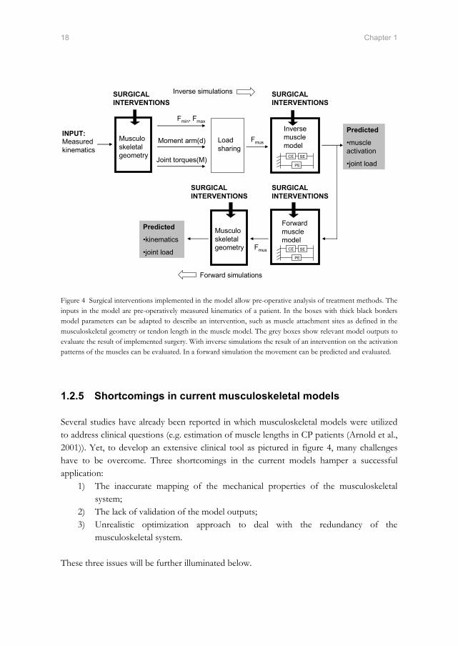
Alterations in the anatomy of the subject as a result of orthopedic interventions can be implemented in a realistic musculoskeletal model by adapting corresponding anatomical model parameters. For example, by changing the 3D position of a tendon attachment on a body segment, a tendon transfer can be implemented. Inverse dynamic simulation of the adapted model shows the effect of virtual interventions on muscle forces, joint forces and muscle activations, under the assumption that the pre-operatively measured input motion of the segments is unchanged after surgery. A forward dynamic simulation allows the clinician to predict the altered movements of a patient after surgery. Activation patterns of the muscles during gait, determined pre-operatively in an inverse analysis, can be used as input to predict the movement of the segments after the intervention (see figure 4). This approach assumes that activation patterns are unchanged after surgery.
18 Chapter 1
Musculo skeletal geometry
Load sharing
Inverse muscle model
Moment arm(d)Measured kinematics
Joint torques(M)
Fmus
Predicted
•muscle activation
•joint load
Fmin, Fmax
Predicted
•kinematics
•joint load
Forward simulations
Inverse simulations
Musculo skeletal geometry
Forward muscle model
Fmus CE SE
PE
CE SE
PE
INPUT:
SURGICAL INTERVENTIONS
SURGICAL INTERVENTIONS
SURGICAL INTERVENTIONS
SURGICAL INTERVENTIONS
Figure 4 Surgical interventions implemented in the model allow pre-operative analysis of treatment methods. The inputs in the model are pre-operatively measured kinematics of a patient. In the boxes with thick black borders model parameters can be adapted to describe an intervention, such as muscle attachment sites as defined in the musculoskeletal geometry or tendon length in the muscle model. The grey boxes show relevant model outputs to evaluate the result of implemented surgery. With inverse simulations the result of an intervention on the activation patterns of the muscles can be evaluated. In a forward simulation the movement can be predicted and evaluated.
1.2.5 Shortcomings in current musculoskeletal models
Several studies have already been reported in which musculoskeletal models were utilized to address clinical questions (e.g. estimation of muscle lengths in CP patients (Arnold et al., 2001)). Yet, to develop an extensive clinical tool as pictured in figure 4, many challenges have to be overcome. Three shortcomings in the current models hamper a successful application:
1) The inaccurate mapping of the mechanical properties of the musculoskeletal system;
2) The lack of validation of the model outputs; 3) Unrealistic optimization approach to deal with the redundancy of the
musculoskeletal system.
These three issues will be further illuminated below.
Introduction 19
1) Mapping of mechanical properties of the musculoskeletal system For successful clinical application, a musculoskeletal model should accurately represent the mechanical properties of the investigated subject. Discrepancies between model and subject lead to inaccurate model outputs and incorrect conclusions about the functioning of the subject’s locomotor apparatus. Several studies have been reported in which certain model parameters were collected directly from magnetic resonance images (MRI) of a subject (e.g. hamstring and adductor moment arms in patients with cerebral palsy (Arnold et al., 2000) or muscle volumes of upper limb muscles in healthy subjects (Holzbaur et al., 2007)). Yet to date, in vivo measurement of a complete and accurate dataset on a subject has been found impracticable. For example sarcomere length, an important parameter required to derive optimal fiber length and corresponding force-length characteristics, is immeasurable in MRI. Other muscle properties are hard to recognize, such as broad muscle attachment sites with fibers attaching directly to the bone (e.g. gluteus maximus). It is impossible to compute important clinical biomechanical measures like joint compression forces and muscle forces with an anatomical dataset based on these imaging methods. To construct a comprehensive musculoskeletal model (e.g. (Glitsch and Baumann, 1997, Anderson and Pandy, 2001, Delp et al., 1990, Heller et al., 2001) generic anatomical datasets are required. The available dataset have two shortcomings. The first shortcoming is the incompleteness of existing anatomical datasets ((Brand and Crowinshield, 1982, Wickiewicz et al., 1983, Friederich and Brand, 1990). For example, Wickiewicz et al. (1983) reported sarcomere length of 27 muscles of the lower extremity together with other muscle parameters. Yet, this is only a part of the total number of muscles acting on the lower extremity. Other important parameters such as joint parameters and muscle attachment sites are absent. Brand et al. (1982) reported muscle attachment sites but lacked for example optimal fiber lengths of the corresponding muscles. Moreover, several parameters have never been measured in any dataset, for example to describe curving of several muscles around intervening structures or to determine the joint angle at which a muscle fiber is at optimal length. In sum, one complete dataset to construct a comprehensive musculoskeletal model is lacking. To obtain a complete set of parameters, different datasets had to be merged and the missing parameters guessed (e.g. (Delp et al., 1990)). This is done such that model outputs like maximal isometric joint moments are in agreement with in vivo data. However, a good fit does not necessary mean an accurate representation of the individual muscle properties as more combinations of muscle forces can produce the same joint torque. Since the effect of scaling and estimation is uncertain, inaccuracies and inconsistencies are inevitable. The resulting dataset represents an anatomical configuration that never existed in which (unknown) interactions between different anatomical parameters are lost, or new interactions are created.
20 Chapter 1
The second shortcoming of the available generic anatomical datasets is the inaccurate discretization of the human locomotor apparatus. Large reductions of the actual morphology cause errors in model output. The mechanical effect of a muscle is often described with only 1 (or in some cases maximal 3) muscle element(s) (Brand and Crowinshield, 1982). However, when a muscle consists of 1 element a muscle can only exert a force to segment. In reality a muscle with fibers attaching directly to the bone (e.g. Soleus) can exert combinations of pulling forces resulting in a torque to the bone. For accurate description of muscles with large attachments sites typically a minimum of 6 muscles is required to describe the mechanical effect of the muscle sufficiently accurate (Van der Helm and Veenbaas, 1991). Furthermore, an insufficient number of muscle elements in a load sharing results in unrealistic equilibration of the external moments. When more elements are defined, only certain parts of the muscle may be activated to avoid unwanted moments with respect to other joint axes. These differentiations within a muscle are not represented with only one muscle element. This results in too high forces in the available muscle elements and too high joint reaction forces (e.g. (Glitsch and Baumann, 1997)). Finally, many muscles that curve around intervening structures are inaccurately represented. These muscles are defined as straight muscle element which results in inaccuracies in muscle moment arm, length and velocity; important parameters for estimation of muscle force. Delp et al. (1990) included ‘via points’ to compensate this shortcoming, yet these model parameters are not based on direct anatomical measurements. When a muscle can freely shift over a bone, this results in an inaccurate description of the muscle moment arm when joint angles are varied. 2) Validation The validation of a model is important to evaluate if the model accuracy fits with the requirements. Yet the available sources for validation are very limited. Typically, to increase resemblance with the subject a generic model is scaled by fitting the bony landmarks of a subject to the bony landmarks defined in the model. Subsequently, the model parameters are proportionally scaled, with the same ratios as the segments. However, the scaling of internal parameters, which are invisible from the outside such as sarcomere length or tendon slack length, is based on assumptions that are unverifiable. The accuracy of these model parameters is unknown. Direct measurement of force in the muscles is impractical so the direct validation of optimized muscle forces is impossible. EMG and in vivo measured joint compression forces are used for the evaluation of the validity of estimated muscle force. Yet these measures are indirect and limited available. 3) Optimization of muscle force The accuracy of muscle forces determined with a musculoskeletal model, and thus a successful model application, is highly dependent on the optimization procedure. To
Introduction 21
investigate the function of a specific muscle during a certain motor task, it is important that the correct amount of force is attributed to the muscle. There are two shortcomings in existing methods which cause inaccuracies in the load sharing. Firstly, in many models a muscle force is bounded between zero and a static maximal force based on muscle PCSA (Glitsch and Baumann, 1997, Crowninshield and Brand, 1981, Heller et al., 2001). Yet, in reality excitation and activation dynamics bound the transitions in muscle force. Excluding of muscle dynamics in the boundaries allows unrealistic muscle force transitions in which a muscle force instantaneously switches between zero and maximal force or visa versa. A second shortcoming is concerned with the cost function used to estimate the muscle force. Many models minimize mechanical cost functions which are based on muscle force (e.g. minimization of the sum of muscle force or the sum of squared muscle stresses; see for an overview (Erdemir et al., 2007)). However, there is no proven relation between these cost functions and the actual distribution of forces over the different muscles. With these mechanical cost functions muscles with large moment arms and large PCSAs are preferred. Small muscles with short fibers and moment arm do not contribute, resulting in unrealistic synergies (Praagman et al., 2006). In summary, it is likely that a physiologically more realistic optimization approach in combination with accurate and consistent model parameters will result in a more accurate estimation of muscle force. This will make the use of a clinical tool as described in figure 4 more feasible.
1.3 Historical framework of this thesis
In 1990 the Laboratory of Biomechanical Engineering was founded at the University of Twente. From the start, gait analysis and musculoskeletal modeling has been an important line of research in the laboratory. This line was initiated with the PhD thesis of Koopman who developed a 3D linked segment model for reconstruction of measured kinematics and analysis of human gait (Koopman, 1989). Thunnissen continued this path and developed a musculoskeletal model of the lower extremity based on the dataset of Brand et al. (1982) consisting of 47 muscle elements (Thunnissen, 1993). The model was used to estimate muscle forces during gait. It was concluded that more accurate anatomical parameters like physiological cross sectional areas and force-length properties were required for further enhancement of muscle force estimation. Van Der Belt (1997) made the step towards forward model simulations. Optimal control was used to simulate walking in the sagittal plane in a linked segment model with active and passive components in the joints (Van der Belt, 1997). In the next years several researchers in the group worked on the modeling of the individual muscles (Yucesoy, 2003, Van der Linden, 1998, Meijer, 1998). Van Der Kooij

22 Chapter 1
(2003) compared muscle forces estimated with the dataset of Brand (1982) and Pierrynowksi (1995) and came, in agreement with Thunnissen (1993), to the conclusion that a more refined dataset is needed. The methodology as used in the Delft Shoulder and Elbow model was suggested (van der Helm, 1994). In this model muscles with large attachment sites are defined with multiple muscle elements. Besides, curved muscle elements are used to describe curving of muscles around bony contours. This resulted in an accurate representation of the mechanical effect of shoulder muscles. Therefore, the next step in the line of research is the collection of a more accurate anatomical dataset. This dataset allows the construction of a new and comprehensive musculoskeletal model in which morphology is accurately defined. This will improve muscle force estimation, which is an important condition for future clinical model applications.
1.4 Thesis aim and outline
The goal of this study is to develop and validate a comprehensive inverse-forward dynamic musculoskeletal model of the lower extremity based on an accurate and consistent anatomical dataset aiming to evaluate if-then scenarios with respect to the treatment of gait disorders. Chapter 2 describes the collection of a consistent anatomical dataset of lower extremity measured on a male embalmed specimen. In Chapter 3 the Twente Lower Extremity Model (TLEM) is presented. This comprehensive musculoskeletal model of the lower extremity model is unique since it is fully based on one measured dataset. Muscle moment arms are calculated and compared with the literature in order to validate the geometry defined in the model. Together with the measured force generating properties, the maximal isometric moments can be calculated. In chapter 4 this model output is compared with maximal voluntary contractions reported in literature as a next and important step in the validation of the model. In chapter 5 the dynamic properties of the model are validated. A novel inverse-forward dynamic optimization and energy related cost function was utilized to solve the load sharing problem. This optimization method includes a forward dynamic muscle model to account for muscle dynamics. Calculated neural outputs are compared with EMG and calculated joint compression forces are compared with in vivo measurements as described in the literature. Chapter 6 describes the application of the TLEM in a clinical study. It is hypothesized that deformations of the femur neck in spina bifida patients are caused by more vertically orientated hip forces as a result of paralysis of hip abductors. The goal of this study is to investigate if the force patterns on the hip in spina bifida patients, determined with the model, are in agreement with this hypothesis. Finally, this thesis is concluded in the general discussion in chapter 7. The added value and limitations of the TLEM are discussed and future work is suggested for further improvements.

Introduction 23
1.5 References
Anderson, F. C.,Pandy, M. G., 1999. A Dynamic Optimization Solution for Vertical Jumping in Three Dimensions. Computer Methods Biomechanics and Biomedical Engineering, 2, 201-231.
Anderson, F. C.,Pandy, M. G., 2001. Static and dynamic optimization solutions for gait are practically equivalent. Journal of Biomechanics, 34, 153-61.
Arnold, A. S., Asakawa, D. J.,Delp, S. L., 2000. Do the hamstrings and adductors contribute to excessive internal rotation of the hip in persons with cerebral palsy? Gait and Posture, 11, 181-90.
Arnold, A. S., Blemker, S. S.,Delp, S. L., 2001. Evaluation of a deformable musculoskeletal model for estimating muscle-tendon lengths during crouch gait. Annals of Biomedical Engineering, 29, 263-74.
Bischoff, E., 1863. Einige Gewichts- und Trocken-Bestimmungen der Organe des menslichen Korpers. Z. rationelle Med., 20, 77–118.
Blemker, S. S.,Delp, S. L., 2005. Three-dimensional representation of complex muscle architectures and geometries. Annals of Biomedical Engineering, 33, 661-73.
Brand, R. A.,Crowinshield, R. D., 1982. A model of lower extremity muscular anatomy. Journal of Biomechanics, 104, 153-161.
Carroll, N. C.,Sharrard, W. J., 1972. Long-term follow-up of posterior iliopsoas transplantation for paralytic dislocation of the hip. Journal of Bone and Joint Surgery, 54, 551-60.
Chandler, R. F., Clauser, C. E., Mcconville, J. T., Reynolds, H. M.,Young, J. W., 1975. Investigation of inertial properties of the human body. Report DOT HS-801430, National Technical Information Service, Springfield Virginia 22151, USA.
Crowninshield, R. D.,Brand, R. A., 1981. A physiologically based criterion of muscle force prediction in locomotion. Journal of Biomechanics, 14, 793-801.
De Zee, M., Hansen, L., Wong, C., Rasmussen, J.,Simonsen, E. B., 2007. A generic detailed rigid-body lumbar spine model. Journal of Biomechanics, 40, 1219-27.
Delp, S. L.,Loan, J. P., 1995. A graphics-based software system to develop and analyze models of musculoskeletal structures. Computers in Biology and Medicine, 25, 21-34.
Delp, S. L., Loan, J. P., Hoy, M. G., Zajac, F. E., Topp, E. L.,Rosen, J. M., 1990. An interactive graphics-based model of the lower extremity to study orthopaedic surgical procedures. IEEE Transactions on Biomedical Engineering, 37, 757-67.
Duffy, C. M., Hill, A. E., Cosgrove, A. P., Corry, I. S., Mollan, R. A.,Graham, H. K., 1996. Three-dimensional gait analysis in spina bifida. Journal of Pediatric Orthopedics, 16, 786-91.
Erdemir, A., Mclean, S., Herzog, W.,Van Den Bogert, A. J., 2007. Model-based estimation of muscle forces exerted during movements. Clinical Biomechanics (Bristol, Avon), 22, 131-54.
Fick, A. E.,Weber, E., 1877. Anatomisch-mechanische Studie ueber die Schultermuskeln I. Verhandl. Würz. Phys. Med. Ges., 11, 123-153.
Fraser, R. K., Hoffman, E. B., Sparks, L. T.,Buccimazza, S. S., 1992. The unstable hip and mid-lumbar myelomeningocele. J Bone Joint Surg Br, 74, 143-6.
Friederich, J. A.,Brand, R. A., 1990. Muscle fiber architecture in the human lower limb. Journal of Biomechanics, 23, 91-5.

24 Chapter 1
Glitsch, U.,Baumann, W., 1997. The three-dimensional determination of internal loads in the lower extremity. Journal of Biomechanics, 30, 1123-31.
Hatze, H. (1981) Myocybernetic control models of skeletal muscle. Pretoria, University of South Africa.
Heller, M. O., Bergmann, G., Deuretzbacher, G., Durselen, L., Pohl, M., Claes, L., Haas, N. P.,Duda, G. N., 2001. Musculo-skeletal loading conditions at the hip during walking and stair climbing. Journal of Biomechanics, 34, 883-93.
Higginson, J. S., Zajac, F. E., Neptune, R. R., Kautz, S. A., Burgar, C. G.,Delp, S. L., 2006. Effect of equinus foot placement and intrinsic muscle response on knee extension during stance. Gait and Posture, 23, 32-6.
Hill, A. V., 1938. The heat of shortening and the dynamic constants of muscle. proc. R Soc Lond B, 126, 136-195.
Holzbaur, K. R., Murray, W. M., Gold, G. E.,Delp, S. L., 2007. Upper limb muscle volumes in adult subjects. Journal of Biomechanics, 40, 742-9.
Huxley, A. F., 1957. Muscle contraction and theories of contraction. Prog Biophys Biochem, 7, 225-318.
Knutsson, E.,Richards, C., 1979. Different types of disturbed motor control in gait of hemiparetic patients. Brain, 102, 405-30.
Koopman, B. (1989) The three-dimensional analysis and prediction of human walking. PhD Thesis, University of Twente, Enschede.
Koopman, B., Grootenboer, H. J.,De Jongh, H. J., 1995. An inverse dynamics model for the analysis, reconstruction and prediction of bipedal walking. Journal of Biomechanics, 28, 1369-76.
Lieber, R. L.,Friden, J., 2001. Clinical significance of skeletal muscle architecture. Clinical Orthopaedics and Related Research, 140-51.
Meijer, K. (1998) Muscle Mechanics - The effect of stretch and shortening on skeletal muscle force., PhD Thesis, University of Twente, Enschede.
Neptune, R. R., Zajac, F. E.,Kautz, S. A., 2004. Muscle force redistributes segmental power for body progression during walking. Gait and Posture, 19, 194-205.
Oomens, C. W., Maenhout, M., Van Oijen, C. H., Drost, M. R.,Baaijens, F. P., 2003. Finite element modelling of contracting skeletal muscle. Philosophical Transactions of the Royal Society of London. Series B: Biological Sciences, 358, 1453-60.
Pandy, M. G., 2001. Computer modeling and simulation of human movement. Annual Review of Biomedical Engineering, 3, 245-73.
Pandy, M. G.,Berme, N., 1988. Synthesis of human walking: a planar model for single support. Journal of Biomechanics, 21, 1053-60.
Pierrynowski, M. R., 1995. Analytic representation of muscle line of action and geometry, in: Allard, P., Stokes, I. A. F. & Blanchi, J. P. (Eds.) Three-Dimensional Analysis of Human Movement. Human Kinetics, Champaign, IL, pp. 214-256.
Praagman, M., Chadwick, E. K., Van Der Helm, F. C.,Veeger, H. E., 2006. The relationship between two different mechanical cost functions and muscle oxygen consumption. Journal of Biomechanics, 39, 758-65.
Root, L., Miller, S. R.,Kirz, P., 1987. Posterior tibial-tendon transfer in patients with cerebral palsy. J Bone Joint Surg Am, 69, 1133-9.
Sharrard, W. J., 1964. Posterior Iliopsoas Transplantation In The Treatment Of Paralytic Dislocation Of The Hip. J Bone Joint Surg Br, 46, 426-44.
Theile, F. W., 1884. Gewichtsbestimmungen zur Entwickelung des Muskelsystems und Skelettes beim Menschen. Ksl. Leop.-Carol.-Deutchen Akad. d. Naturforscher, 46, 139–471.

Introduction 25
Thelen, D. G., Anderson, F. C.,Delp, S. L., 2003a. Generating dynamic simulations of movement using computed muscle control. Journal of Biomechanics, 36, 321-8.
Thelen, D. G., Anderson, F. C.,Delp, S. L., 2003b. Generating dynamic simulations of movement using computed muscle control. Journal of Biomechanics, 36, 321-8.
Thunnissen, J. (1993) Muscle force prediction during human gait. PhD Thesis, University of Twente, Enschede.
Tsirakos, D., Baltzopoulos, V.,Bartlett, R., 1997. Inverse optimization: functional and physiological considerations related to the force-sharing problem. Critical Reviews in Biomedical Engineering, 25, 371-407.
Van Der Belt, D. (1997) Simulation of walking using Optimal Control. PhD Thesis, University of Twente, Enschede.
Van Der Helm, F. C., 1994. A finite element musculoskeletal model of the shoulder mechanism. Journal of Biomechanics, 27, 551-69.
Van Der Helm, F. C.,Veenbaas, R., 1991. Modelling the mechanical effect of muscles with large attachment sites: application to the shoulder mechanism. Journal of Biomechanics, 24, 1151-63.
Van Der Kooij, H., Jacobs, R., Koopman, B.,Grootenboer, H., 1999. A multisensory integration model of human stance control. Biological Cybernetics, 80, 299-308.
Van Der Linden, B. (1998) Mechanical modeling of skeletal muscle functioning. Simulation of walking using Optimal Control.
Verdaasdonk, B. W., Koopman, H. F.,Helm, F. C., 2005. Energy efficient and robust rhythmic limb movement by central pattern generators. Neural Netw.
Weber, E., 1851. Über die langenverhaltnisse der fleischfasern der muskeln im algemeinen. Berichte u. d. Verh. d. Konigl. Sachs. Ges. d. Wiss. Math.-Phys. CL., 5-86.
Wickiewicz, T. L., Roy, R. R., Powell, P. L.,Edgerton, V. R., 1983. Muscle architecture of the human lower limb. Clinical Orthopaedics, 275-83.
Woittiez, R. D., Huijing, P. A., Boom, H. B.,Rozendal, R. H., 1984. A three-dimensional muscle model: a quantified relation between form and function of skeletal muscles. Journal of Morphology, 182, 95-113.
Yamaguchi, G. T., Sawa, A. G. U., Moran, D. W., Fessler, M. J.,Winters, J. M., 1990. A survey of human musculotendon actuator parameters, in: Winter, J. M. & Woo, S. L. Y. (Eds.) Multiple Muscle Systems: Biomechanics and Movement Organisation. Springer, Berlin, pp. 717-773.
Yucesoy, C. (2003) Intra-,inter- and extramuscular myofascial force transmission. PhD Thesis, University of Twente, Enschede.
Yucesoy, C. A., Koopman, B. H., Huijing, P. A.,Grootenboer, H. J., 2002. Three-dimensional finite element modeling of skeletal muscle using a two-domain approach: linked fiber-matrix mesh model. Journal of Biomechanics, 35, 1253-62.
Zajac, F. E., 1989. Muscle and tendon: properties, models, scaling, and application to biomechanics and motor control. Critical Reviews in Biomedical Engineering, 17, 359-411.


Chapter 2
Morphological muscle and joint parameters for
musculoskeletal modelling of the lower extremity
M.D. Klein Horsman, H.F.J.M. Koopman, F.C.T. van der Helm, L. Poliacu Prosé, H.E.J. Veeger Clinical Biomechanics 22: 239-247, 2007

Abstract
To assist in the treatment of gait disorders, an inverse and forward 3D musculoskeletal model of the lower extremity will be useful that allows to evaluate if-then scenarios. Currently available anatomical datasets do not comprise sufficiently accurate and complete information to construct such a model. The aim of this paper is to present a complete and consistent anatomical dataset, containing the orientations of joints (hip, knee, ankle and subtalar joints), muscle parameters (optimum length, physiological cross sectional area), and geometrical parameters (attachment sites, ‘via’ points). One lower extremity, taken from a male embalmed specimen, was studied. Position and geometry were measured with a 3D-digitizer. Optotrak was used for measurement of rotation axes of joints. Sarcomere length was measured by laser diffraction. A total of 38 muscles were measured. Each muscle was divided in different muscle lines of action based on muscle morphology. 14 Ligaments of the hip, knee and ankle were included. The presented anatomical dataset embraces all necessary data for state of the art musculoskeletal modelling of the lower extremity. Implementation of these data into an (existing) model is likely to significantly improve the estimation of muscle forces and will thus make the use of the model as a clinical tool more feasible.

Morphological parameters for musculoskeletal modeling 29
2.1 Introduction
Several musculoskeletal models have been developed to study for example gait, jumping or cycling (Zajac, 1989, Pandy, 2001). Most models reviewed by Pandy (2001) and Zajac (1989) are simple 2D models that can be used to gain insight in the principles of control of movement and the role of its components. To study the function of specific muscles for certain tasks more large scale musculoskeletal models are being used, for example to assist in the treatment of gait disorders by studying orthopedic surgical procedures (Delp et al., 1990, Arnold et al., 2001). Arnold et al. (2001) estimated muscle tendon length of the hamstrings and psoas muscles of subjects with cerebral palsy, which is an important parameter in order to predict the biomechanical effect of a surgical intervention. Delp et al. (1990) studied the effect of a tendon transfer and lengthening by adjusting model parameters according to surgical techniques. For studies focusing on the evaluation of specific, clinically relevant, questions, an accurate description of the geometry of the muscles and joints involved is important. The geometry of the musculoskeletal system defines the moment arms and the length of the muscles and thus the moment a muscle can generate at a joint given a muscle force. With this length of the musculotendon complex and geometric muscle parameters such as optimal fiber length, physiological cross sectional area (PCSA), the maximal muscle force can be estimated and used as a constraint in an optimisation to determine the actual muscle force for a specific movement or task. To date, several anatomical studies have been published containing information on the modelling parameters for the lower extremity, containing for example muscle attachments sites (Pierrynowski, 1995, Brand and Crowinshield, 1982) or muscle parameters (Wickiewicz et al., 1983, Spoor et al., 1991, Weber, 1851, Friederich and Brand, 1990). Unfortunately, none of these sets are complete, which implies that when constructing a complete musculoskeletal model different datasets have to be combined or missing parameters have to be estimated. The study presented here is part of a larger project that aims to develop a model that allows clinicians to evaluate if-then scenarios with respect to treatment methods. For this, a complete anatomical dataset will be necessary. Such a set should comprise data on joint properties, muscle actuation parameters and geometrical information, all from the same specimen.

30 Chapter 2
2.2 Methods & results
Measurements were performed on a right lower extremity of a male embalmed specimen (age 77, height 1.74m, weight 105 kg). Pre-experimental selection of the cadaver took place based on physical appearance. The specimen has a relatively high muscle mass and a high fat percentage for the upper body. The cadaver was divided at the level of L1, so the attachment site of the psoas major could be measured. The specimen was fixed in a stainless steel frame, allowing easy positioning (Figure 1). Four reference pins for measuring changes in orientation and position were placed in each of the body segment. The foot was defined as a system with three segments: hindfoot, midfoot and phalanges. These segments were constructed using k-wires. Due to the position during fixation the ‘resting’ position of the leg was with the hip externally rotated, the knee extended with the patella in the corresponding position and the foot in plantar flexion and supination. Position was measured with a 3D-palpator (Pronk and van der Helm, 1991), which is a 3D-digitiser used for this type of measurements with a standard deviation of 1 mm per coordinate. Although it falls outside the scope of this study, it is worth mentioning that prior to the dissection of the specimen, magnetic resonance images (MRI) were acquired for future evaluation of MRI-extracted parameters.
Figure 1 Experimental setup with specimen fixed in frame.

Morphological parameters for musculoskeletal modeling 31
2.2.1 Inertial parameters
Before dissection, anthropometric measurements were performed for estimation of inertial parameters (Clauser et al., 1969, Koopman, 1989). Segment mass and center of mass were calculated using regression equations of respectively Clauser et al. (1969) and Koopman (1989). Moments of inertia were calculated about the transversal and longitudinal axis of the segment (Yeadon and Morlock, 1989). See table 1. Table 1 Segment moments of inertia about the transversal (It) and longitudinal axis (Il) in kg m2, segment mass (kg) and center of mass with respect to the global frame with the leg in original fixated position (cm).
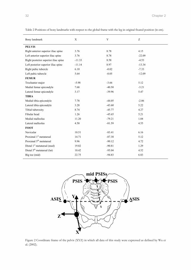
2.2.2 Palpable bony landmarks and reference pins
Prior to dissection 19 palpable bony landmarks were measured on the skin (see table 2) with the leg in the original fixated , or ‘reference’ position, together with the tips of the reference pins such that future local coordinate systems could be constructed. The choice of landmarks was based on the definition of local coordinate frames as described by the Standardization and Terminology Committee of the International Society of Biomechanics (Wu et al., 2002). To facilitate interpretation, all data presented in this study were subsequently expressed in the coordinate frame of the pelvis (figure 2), with the hip center as origin and the axes defined as follows: (Wu et al., 2002) Z: The line parallel to a line connecting the right and left anterior superior iliac spine
(ASIS), and point to the right. X: The line parallel to a line lying in the plane defined by the two ASISs and the
midpoint of the right and left posterior superior iliac spine (PSIS), orthogonal to the Z-axis, pointing anteriorly.
Y: The line perpendicular to X and Z, pointing cranially.
Segment It Il Mass X Y Z
Pelvis 0.012 0.017 3.18 1.40 5.40 -8.92 Femur 0.197 0.058 11.54 3.70 -15.62 -0.44 Tibia 0.058 0.007 4.00 7.57 -57.00 1.75 Foot 0.005 0.001 1.30 10.48 -88.14 1.14
32 Chapter 2
Table 2 Positions of bony landmarks with respect to the global frame with the leg in original fixated position (in cm).
Figure 2 Coordinate frame of the pelvis (XYZ) in which all data of this study were expressed as defined by Wu et al. (2002).
Bony landmark X Y Z
PELVIS Right anterior superior iliac spine 3.76 8.78 4.15 Left anterior superior iliac spine 3.76 8.78 -22.09 Right posterior superior iliac spine -11.33 8.58 -4.53 Left posterior superior iliac spine -11.14 8.97 -13.34 Right pubic tubercle 6.10 -0.02 -7.33 Left pubic tubercle 5.64 -0.05 -12.09 FEMUR Trochanter major -5.98 -3.66 5.12 Medial femur epicondyle 7.68 -40.50 -3.21 Lateral femur epicondyle 3.17 -39.96 5.47 TIBIA Medial tibia epicondyle 7.78 -44.05 -2.06 Lateral tibia epicondyle 3.28 -43.60 5.22 Tibial tuberosity 8.74 -45.77 4.27 Fibular head 1.26 -45.65 5.21 Medial malleolus 11.20 -79.21 1.04 Lateral malleolus 4.50 -81.59 4.55 FOOT Navicular 10.51 -83.41 6.16 Proximal 1st metatarsal 14.71 -87.38 5.12 Proximal 5th metatarsal 9.96 -90.12 4.72 Distal 1st metatarsal (med) 19.82 -90.81 1.29 Distal 5th metatarsal (lat) 10.42 -95.04 4.52 Big toe (mid) 22.75 -94.83 6.83
X
Y
Z
ASIS
PSIS PSIS mid PSISs
ASIS
Morphological parameters for musculoskeletal modeling 33
Since it was impossible to measure all anatomical structures without segmenting the leg, coordinates of the anatomical structures were always collected together with the tips of the reference pins in each session. These data were then rotated and translated to the ‘reference’ position, using the actual position of the reference pins and the position of these pins in the original position (Veldpaus et al., 1988). The error, as described by Veldpaus et al. (1988), is in the order of 1 mm per coordinate for each session.
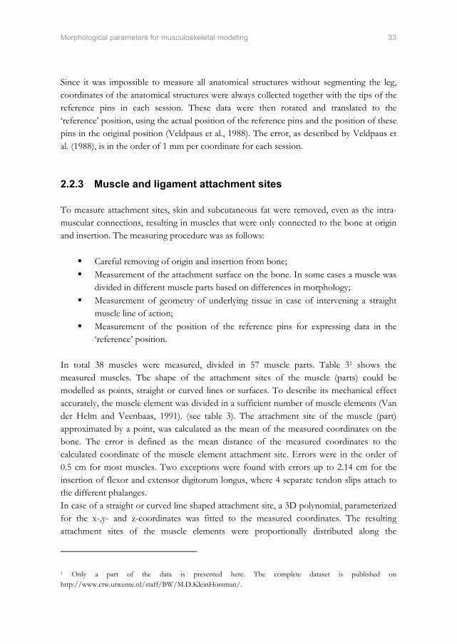
2.2.3 Muscle and ligament attachment sites
To measure attachment sites, skin and subcutaneous fat were removed, even as the intra-muscular connections, resulting in muscles that were only connected to the bone at origin and insertion. The measuring procedure was as follows:
Careful removing of origin and insertion from bone; Measurement of the attachment surface on the bone. In some cases a muscle was
divided in different muscle parts based on differences in morphology; Measurement of geometry of underlying tissue in case of intervening a straight
muscle line of action; Measurement of the position of the reference pins for expressing data in the
‘reference’ position.
In total 38 muscles were measured, divided in 57 muscle parts. Table 31 shows the measured muscles. The shape of the attachment sites of the muscle (parts) could be modelled as points, straight or curved lines or surfaces. To describe its mechanical effect accurately, the muscle element was divided in a sufficient number of muscle elements (Van der Helm and Veenbaas, 1991). (see table 3). The attachment site of the muscle (part) approximated by a point, was calculated as the mean of the measured coordinates on the bone. The error is defined as the mean distance of the measured coordinates to the calculated coordinate of the muscle element attachment site. Errors were in the order of 0.5 cm for most muscles. Two exceptions were found with errors up to 2.14 cm for the insertion of flexor and extensor digitorum longus, where 4 separate tendon slips attach to the different phalanges. In case of a straight or curved line shaped attachment site, a 3D polynomial, parameterized for the x-,y- and z-coordinates was fitted to the measured coordinates. The resulting attachment sites of the muscle elements were proportionally distributed along the
1 Only a part of the data is presented here. The complete dataset is published on http://www.ctw.utwente.nl/staff/BW/M.D.KleinHorsman/.

34 Chapter 2
polynomial. Based on Van der Helm & Veenbaas (1991), for a first order polynomial at least 2 attachment sites and for a higher order polynomial at least 3 attachment sites were defined. The error of the 3D polynomial fit, defined as the mean distance of the data points to the polynomial, had a maximal value of 0.46 cm for the origin of the lateral part of the soleus. For a surface attachment site, the measured coordinates were defined as a plane (Van der Helm et al., 1992), where the measured coordinates were projected on that plane. The circumference of the projected coordinates could define an area, divided in 3 equal parts. For each part, 2 elements were proportionally distributed over the area resulting in 6 points describing the surface. For surface shaped attachment sites the error was defined as the mean distance of the measured coordinates to the optimized plane. It had a maximal value of 0.42 cm for the origin of the gluteus minimus. The above process resulted in a total of 163 muscle elements for the 58 muscle parts as described in Table 3 and the Web Supplementary Material (WSM) 1. 14 Ligaments of the hip, knee and ankle joint were measured (Table 4). Ligaments were considered as a straight line between origin and insertion.
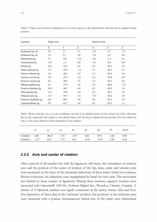
2.2.4 Bony contours and via points
In case of a curvature of the muscle line of action due to underlying structures, two methods were used to describe this change in muscle force direction. If a muscle line of action was intervened by the surface of an underlying bone and the muscle was free to shift over this surface, the resulting curved line of action was defined around this bony contour using a mathematical representation of this bone (Van der Helm et al., 1992). In that case the surface was digitized and a geometric shape was fitted to the measured data points using an optimization described by Van der Helm et al. (1992b). This resulted in two relevant geometries (table 5). Cylinder 1, representing the femur condyle, is meant to describe the curved line of action of the gastrocnemius around this structure. The second cylinder describes the curve of the iliopsoas around the pubis of the pelvis. For 19 other muscle (parts) a curvature of the line of action was observed but a free shift of the muscle over the underlying structure was not possible, as in tibialis posterior, or in sartorius. In these cases ‘via’ points were defined, dividing the involved muscle in series of straight line segments (Delp et al., 1990). See WSM.

Morphological parameters for musculoskeletal modeling 35
Table 3 Per muscle part: origin, insertion described as surface, line(order) or point, divided in a number of elements and the muscle parameters: PCSA, optimal fiber length(Lopt), tendon length(Lten), mass and pennation angle. A muscle line can be straight (S), curving around a bony contour (BC) or consist of via points (VP).
Muscle Origo Ins. # elem. S, BC or VP
PCSA (cm2)
Lopt (cm)
Lten (cm)
Mass (g)
Pen. ang.(º)
Add. brev. (prox.) S 3.8 9.5 0 38.3 0 Add. brev. (mid) S 3.5 10.4 0 38.3 0 Add. brev. (dist)
Surf. Line(3) 6 S 3.2 11.2 0 38.3 0
Add. long. Line(3) Line(3) 6 S 15.1 10.6 0 168.5 0 Add. magn. (dist.) Point Line(2) 3 S 26.5 10.8 4.2 302.0 0 Add. magn. (mid.) Surf. Line(3) 6 S 22.1 10.4 0 243.0 0 Add. magn. (prox.) Line(1) Line(1) 4 S 5.0 10.7 0 56.0 0 Bic. fem. CL Point Point 1 S 27.2 8.5 13.0 245.0 30 Bic. fem. CB Line(3) Point 3 S 11.8 9.1 3.1 114.0 0 Ext. dig. long. Line(2) Point 3 VP 5.4 6.0 30.1 34.1 8 Ext. hal. long. Line(2) Point 3 VP 6.1 6.0 17.8 38.3 14 Flex. dig. long. Surf. Point 3 VP 6.6 3.8 16.6 26.7 28 Flex. hal. long. Surf. Point 3 VP 31.1 2.6 23.4 83.7 30 Gastrocn. (lat.) Point Point 1 BC 24.0 5.7 23.4 144.0 25 Gastrocn. (med.) Point Point 1 BC 43.8 6.0 21.2 278.0 11 Gemellus (inf.) Point Point 1 S 4.1 3.4 0 15.0 0 Gemellus (sup.) Point Point 1 S 4.1 3.4 0 15.0 0 Glut. max. (sup.) Surf. Surf. 6 S 49.7 12.0 0 629.0 0 Glut. max. (inf.) Surf. Line(2) 6 S 22.5 15.1 0 360.0 0 Glut. med. (ant.) Surf. Surf. 6 S 37.9 3.8 0 152.5 0 Glut. med. (post.) Surf. Surf. 6 S 60.8 4.5 3.0 287.0 16 Glut. min. (lat.) S 10.0 2.8 7.3 29.1 0 Glut. min. (mid.) S 8.1 3.4 7.3 29.1 0 Glut. min. (med.)
Surf. Point 3 S 7.4 3.7 7.3 29.1 0
Gracilis Line(1) Point 2 VP 4.9 18.1 14.0 92.9 0 Iliacus (lat.) Surf. Point 3 BC 6.6 10.3 11.3 71.5 26 Iliacus (mid.) Surf. Point 3 BC 13.0 5.2 11.3 71.5 0 Iliacus (med.) Surf. Point 3 BC 7.6 8.9 15.5 71.5 0 Obt. ext. (inf.) Line(1) Point 2 S 5.5 6.9 3.5 40.0 0 Obt. ext. (sup.) Surf. Point 3 VP 24.6 2.8 3.0 72.0 0 Obturator int. Surf. Point 3 VP 25.4 2.1 8.2 55.0 0 Pectineus Line(1) Line(1) 4 S 6.8 11.5 0 82.4 0 Peroneus brev. Surf. Point 3 VP 19.0 2.7 6.4 53.9 23 Peroneus long. Surf. Point 3 VP 23.9 3.4 15.9 86.0 16 Peroneus tert. Line(2). Point 3 VP 6.2 4.3 10.0 28.0 19 Piriformis Point Point 1 S 8.1 3.9 1.6 33.0 0 Plantaris Point Point 1 S 2.4 4.8 35.0 12.0 0 Popliteus Point Line(1) 2 VP 10.7 2.4 1.0 27.0 0 Psoas minor Point Point 1 S 1.1 5.9 15.2 7.0 0 Psoas major Surf. Point 3 BC 19.5 9.9 11.3 204.0 13 Quadratus fem. Line(1) Line(1) 4 S 14.6 3.4 0 52.0 0 Rectus fem. Point Line(1) 2 S 28.9 7.8 9.6 239.0 22 Sartorius (prox.) Point Point 1 VP 5.9 34.7 7.9 217.0 0 Sartorius (dist.) Point Point 1 VP 5.9 34.7 7.9 217.0 0 Semimembr. Point Point 1 S 17.1 8.1 15.7 146.0 25 Semitend. Point Point 1 VP 14.7 14.2 23.7 220.0 0 Soleus (med.) Line(2) Point 3 S 94.3 2.4 8.5 238.5 64 Soleus (lat.) Line(2) Point 3 S 85.9 2.6 8.5 238.5 59 Tensor fasc. l. Line(1) Point 2 S 8.8 9.5 0 88.0 0 Tibialis ant. Surf. Point 3 VP 26.6 4.6 23.5 129.0 10 Tibialis post. (med.) Surf. Point 3 VP 21.6 2.4 11.0 55.9 25 Tibialis post. (lat.) Surf. Point 3 VP 21.6 2.4 11.0 55.9 43 Vastus interm. Surf. Line(1) 6 S 38.1 7.7 12.6 309.0 12 Vastus lat. (inf.) S 10.7 4.2 9.6 48.0 0 Vastus lat. (sup.) Surf. Line(2) 6 S 59.0 9.1 9.6 568.0 0 Vastus med. (inf.) S 9.8 7.6 9.6 78.0 0 Vastus med. (mid.) S 23.2 7.6 9.6 186.0 0 Vastus med. (sup.)
Surf. Line(2) 6 S 26.9 8.3 9.6 236.0 0
36 Chapter 2
Table 4 Origin and insertion of ligaments in cm with respect to the global frame with the leg in original fixated position.
Table 5 Bony contours. sx, sy, sz are coordinates (in cm) of an arbitrary point on the central axis with a direction [dx dy dz], expressed with respect to the global frame with the leg in original fixated position. R is the radius (in cm), e is the mean distance of the datapoints to the cylinder.
2.2.5 Axis and center of rotation
After removal of all muscles but with the ligaments still intact, the orientation of rotation axes and the position of the center of rotation of the hip, knee, ankle and subtalar joint were measured on the basis of the kinematic behaviour of these joints. Endo/exo rotation, flexion/extension, ab/adduction were manipulated by hand for each joint. The movement was limited by bone contact or ligaments. During these motions, segment motions were measured with Optotrak® (100 Hz, Nothern Digital Inc., Waterloo, Ontario, Canada). A cluster of 4 Optotrak markers was rigidly connected on the pelvis, femur, tibia and foot. For expression of these data in the ‘reference’ position, the positions of the reference pins were measured with a pointer. Instantaneous helical axis of the joints were determined
Ligament Origin (cm) Insertion (cm)
X Y Z X Y Z Iliofemoral lig. ant. 2.0 3.1 1.1 -2.2 -3.7 1.2 Iliofemoral lig. lat. 1.2 3.3 2.0 -3.9 -1.4 4.0 Pubofemoral lig. 2.7 -0.6 -3.6 -4.0 -1.4 4.1 Ischiofemoral lig. -2.9 -1.3 0.0 -4.1 -0.4 0.9 Patellar lig. 10.2 -39.7 3.6 8.5 -45.5 3.8 Tibial collateral lig. 7.6 -39.6 -3.2 7.5 -48.4 0.1 Fibular collateral lig. 3.0 -40.3 5.0 1.2 -45.4 4.3 Anterior cruciate lig. 5.8 -41.2 -0.1 6.2 -41.8 0.9 Posterior cruciate lig. 4.4 -40.3 1.2 3.5 -43.3 0.2 Oblique popliteal lig. 3.3 -37.9 3.0 3.5 -44.0 -2.3 Posterior tibiotalar lig. 10.2 -80.1 0.4 8.2 -80.5 1.0 Tibiocalcaneal lig. 11.1 -79.8 1.0 9.6 -82.5 1.0 Tibionavicular lig. 11.7 -79.7 1.9 11.9 -83.6 3.5 Posterior talofibular lig. 6.8 -80.7 5.0 6.6 -81.0 2.0 Calacaneofibular lig. 5.9 -81.7 4.4 4.2 -83.5 1.3
sx sy sz dx dy dz R e(cm)
Cylinder 1 6.06 -40.22 -1.75 -0.37 0.04 0.93 2.46 0.05 Cylinder 2 -1.27 0.97 -1.75 0.21 -0.14 -0.79 3.99 0.10

Morphological parameters for musculoskeletal modeling 37
from the position data of the marker clusters (Woltring, 1990, Veeger et al., 1997). Rotation centers and axes are described by respectively the pivot point and optimal direction vector (Woltring, 1990). The error e of the estimation of the rotation center and axis was calculated successively as (Veeger et al., 1997):
)(11∑=
−=N
iioptp PPnorm
Ne (1a)
)'arccos(11∑=
⋅=N
iioptv VV
Ne (1b)
See Table 5 for the direction of the rotation axes and the position of the rotation centers with the corresponding error. The movement of the patella could be approximated as a rotation of this segment with respect to the femur. For the determination of the rotation center and axis, 3 Optotrak markers were mounted on the patella in addition to the 4 markers on the femur. To account for the effect of the quadriceps muscles, an isometric spring was attached to the tendon of the quadriceps and the anterior superior iliac spine to keep the tendon under tension during knee flexion. The mean position of the 3 markers during knee flexion could be described with a circular shaped polynomial. These data points were fitted onto a plane and a circle was fitted on the resulting coordinates. The normal vector of the plane was then defined as the rotation axis and the center of the circle as the rotation center (Table 6). As can be seen these values differ from the knee axis and rotation center. The mean distance of the measured data points to the estimated plane was 0.09 cm. The mean distance to the circle was 0.02 cm. After the separation of segments, a raster of evenly distributed points was measured on the surface of the femoral head and a sphere was fitted to the points on the articular surface. The position of the center of this sphere can be used as a second estimation of the rotation center of the hip joint. The mean distance e of a data point to the calculated sphere is defined as a measure for the accuracy of the optimization (Table 6).

38 Chapter 2
Table 6 Estimated rotation centers (in cm) and rotation axes expressed in the global frame with the leg in original fixated position. Hip rotation center is based on a spherical fit through the surface of the femoral head. Knee, ankle and subtalar rotation axis and center with the corresponding error e (Equation 1) are based on instantaneous helical axis calculations as described by Veeger et al. (1997). The femur-patella joint is based on a circular fit through the trajectory of the patella with respect to the femur.
2.2.6 Muscle parameters
The dissected muscles were weighed, after removing of the tendon, fat and excessive connective tissue, using a scale with an accuracy of 0.1 g. Belly, tendon and muscle fiber length were measured with the palpator, by calculating the distance between begin and end point. The length of at least five representative fibers was measured depending on the size of the muscle. Standard deviation (SD) in fiber length within a muscle was around 0.5 cm for most muscle parts as can be found in the WSM. Exceptions were measured in the gluteus maximus, extensor digitorum longus, add. magnus and gracilis muscle (SD up to 4.7 cm). The pennation angle was determined using the palpator by calculating the angle of the direction at least five muscle fibers with the estimated line of action of the muscle. The vectors were defined by the difference between measured begin and end point. Pennation angles were measured in 20 of the 58 measured muscle parts. Standard deviations within the muscle parts were in the order of 4º. For the other muscle parts pennation angles were small and considered zero. Sarcomere length, needed for determining optimal fiber length, was measured with a He-Ne laser (Young et al., 1990). By positioning a fiber in the 1 mm beam at a fixed distance from a scale, the diffraction pattern, representing the sarcomere length, can be read directly. Fibers were isolated using a microscope (magnitude 20x). The resolution was 0.05 µm depending on the quality of the embalmed fiber. In general from a muscle 6 samples of 6 fibers were measured depending on the size of the muscle. For the smaller muscles a minimum of 3 fibers were measured and for larger muscles like the m. vastus lateralis up to 10 fibers were isolated for diffraction.
Rotation center X Y Z e(cm)
Hip 0 0 0 0.02 Knee 3.84 -40.78 1.38 0.79 Femur-patella 3.51 -38.51 1.90 0.02 Ankle 9.33 -81.36 3.14 0.37 Subtalar 10.87 -80.61 3.36 0.37
Rotation axis X Y Z e(deg)
Knee -0.528 -0.107 0.843 4.73 Femur-patella -0.465 0.024 0.0885 0.09 (cm) Ankle -0.730 -0.206 0.652 6.36 Subtalar -0.780 -0.223 -0.584 8.63
Morphological parameters for musculoskeletal modeling 39
The optimal fiber length of a muscle (part) was calculated as the mean of the actual muscle fibers length for a muscle multiplied by the ratio of the optimal sarcomere length of 2.7 µm (Walker and Schrodt, 1974) and the mean sarcomere lengths of the fibers of that muscle. PCSA at optimal muscle length was defined as the muscle volume divided by the optimal fiber length, where muscle volume is defined as muscle mass divided by its density (1.056 g/cm3 (Klein Breteler et al., 1999)). Largest PCSA (82.6 cm2) was determined for the soleus muscle due to relatively small fiber length. Tendon PCSA was determined by calculating the area of a circular, ellipsoid or rectangular assumed cross section using the measured width and breadth of a tendon area (see WSM).
2.3 Discussion
This study generated a unique anatomical dataset comprising all necessary data for musculoskeletal modelling of the lower extremity. It contains attachment sites of all the muscles of the lower extremity and if necessary the muscle is split up in different muscle elements to describe the mechanical effect more accurate. For each element the important muscle parameters for the estimation of force generating properties are given such as optimal fiber length. Also the joint parameters of the hip, knee, ankle and subtalar joint are included. The expression of all geometrical parameters, in combination with the bony landmarks in the same ‘reference’ frame allows for expression in other local coordinate frames. The presented data form one consistent dataset, which is a major advantage. When different datasets are used to construct a model, scaling between datasets is necessary to correct for inter-individual anatomical variations. The effect of scaling however is uncertain and inaccuracies and inconsistencies are inevitable. The combined datasets result in an anatomical configuration that never existed. In that case (unknown) interactions between different anatomical parameters could get lost. The complete dataset presented in this study is based on one cadaver, which results in a consistent dataset. Attachment sites were represented by a number of coordinates depending on size. For line and surface attachments the error was small (< 0.46 cm). Attachment sites of relatively long tendons to the bone were represented by a point. Some of these attachment sites had relatively large errors, e.g. the insertion of the semimembranosus (e=0.81 cm). Because these tendons cannot exert a moment to the bone (Van der Helm and Veenbaas, 1991), a point attachment site was still seen as an acceptable representation, despite the relatively large error. With the distance between its origin and insertion, the length of a ligament can be calculated in ‘reference’ position. The utilization of these data is limited in models that take stresses in ligaments into account. With the stress-strain relation of the ligament, the stress could be estimated given a certain initial stress and change of length. The calculated ligament lengths however contain small errors due to model assumptions that lead to very large errors in stresses. Secondly, the initial stress in the ligaments in the ‘reference’ position is unknown.

40 Chapter 2
Several groups reported fiber lengths in muscles of the lower extremity (Yamaguchi et al., 1990). A few groups measured sarcomere length for a limited number (max. 27) of leg muscles to calculate optimal fiber length (Spoor et al., 1991, Wickiewicz et al., 1983). In this study we reported optimal fiber lengths for 58 muscle parts. The measured actual fiber length show small standard deviations within a muscle part. If larger variations occurred as in the iliacus, the muscle was split up in different parts. The optimal fiber length was based on sarcomere length measurements using laser diffraction, a very accurate method for measuring sarcomere lengths. Mean sarcomere lengths were found between 2 and 3.7 µm, which is a range consistent with the sliding filament theory according to Walker and Schrodt (1974). This makes it likely that filament length did not change as a result of the embalming process. This assumption is strengthened by the results of a study in rats in which the length change of muscle fibers in muscles fixed intact on the skeleton appeared to be negligible as a result of an embalming process (Cutts, 1988). The isolation of a fiber from a muscle part did not change the sarcomere length as observed in other studies (Klein Breteler et al., 1999). For a few samples no diffraction pattern was observed. It is assumed that this was caused by broken filaments due to embalming process or rigor mortis. These samples were considered as artefacts and were further ignored. PCSA, calculated in this study as muscle volume divided by optimal fiber length, is an important parameter for the estimation of relative force distribution in musculoskeletal models. To have a good estimation of the relative muscle force, PCSA should be determined using one method and based on one cadaver. A comparison with other datasets based on different calculation methods and specimens is difficult. The exact calculation procedure however is less important than the use of a consistent dataset. When pennation angles are compared to the datasets reviewed by Yamaguchi et al. (1990), there are 2 muscles that show large differences. In the present study, pennation angles up to 64 degrees were found for the medial part the soleus in contrary to the study of Friederich and Brand in which a pennation angle of 32 degrees was reported for the soleus muscle (Friederich and Brand, 1990) in contrary to angles up to 64 degrees for the medial part the soleus which found in the present study. Wickiewicz et al. (1983) however reported areas in the soleus muscle up to 60 degrees, which is comparable to our results. Yamaguchi only reports one pennation angle for the tibialis posterior, in this study a lateral part is defined as an extra element with larger angles (43 degrees). The accuracy of rotation centers and axes is crucial in terms of kinematics and kinetics. The hip joint is characterized as a ball-and socket joint and its rotation center can be estimated using a kinematic or geometric approach. Kinematic joint center and axes were constructed from motion data. A reconstruction of the hip joint rotation center by calculation of the optimal pivot point is shown in Figure 3. The mean distance of each helical axis to the pivot point is 0.85 cm. A comparison with the geometric rotation center could not be made due to a missing reference point. However, as for the glenohumeral joint, it is very likely that both

Morphological parameters for musculoskeletal modeling 41
−40 −30 −20 −10 0 10 20 30 40
−40
−30
−20
−10
0
10
20
30
40
Z (cm)
Y (
cm)
Optimal pivot point
Flexion/extension
Endo/exorotation
Ab/adduction
Figure 3 Frontal view of hip rotation center, defined as the optimal pivot point, calculated with instantaneous helical axes of recorded hip rotations around three anatomical axes. methods come up with comparable results (Veeger, 2000). When the geometric rotation center is compared with an estimated hip joint center based on regression equations using bony landmarks (Leardini et al., 1999, Bell et al., 1990), the calculated difference of 1.60 cm is within the range described by Leardini et al. (1999). We considered the knee, ankle and subtalar joint in this study as a hinge with a fixed position and orientation. In reality these joint axes will alter during the arc of motion (e.g. (Lundberg et al., 1989) for the ankle joint) as can be seen in the error for the determination of the rotation axes. The error for the estimation of the rotation center of the knee was larger than the error for the ankle and subtalar axis. This was mainly caused by the translation of the knee rotation center due to rotation of the condyle of the femur over the tibia plateau. This movement of the femur condyle with respect to the tibia plateau is constrained by ligaments and menisci. This explained the difference in the axis of the cylinder fitted on the femur condyle and the optimal knee axis during a knee flexion (table 5 and 6). With a plane and circle fit, a rotation axis and center of the patella with respect to the femur can be estimated with a high accuracy. The calculation of instantaneous helical axes did not lead to accurate results because rotations round the longitudinal axis of the patella occurred. These rotations were due to the lack of the stabilizing effect of the surrounding muscles. By taking the mean position of the 3 markers, this irrelevant effect was not taken into account and only the translation in the sagittal plane was used. For musculoskeletal modelling the position of the attachment sites of the quadriceps on the patella is an important factor for calculation of the moment arm of these muscles during knee flexion. Rotations of the relatively small patella round its longitudinal

42 Chapter 2
axis will have small effects on the position of the attachment site. We believe that the position can be estimated sufficiently accurate with the used method. The dataset in this study comprises the geometry of one, unique, individual. Scaling of data to a particular patient or subject to adapt the model to the anatomy of that subject has an uncertain effect. MRI can be used to collect subject specific parameters, but only to a limited extent. Recognition of attachment sites on the bone and fiber orientation is still difficult in MR images, which makes the calculation of muscle lines of action arbitrary, at least. In addition, MRI data can at this point only produce geometry data, while important parameters for muscle force estimation such as optimal fiber length will still be based on cadaver data. The development of subject specific models comprising all the anatomic parameters of the subject will be one of the future challenges in musculoskeletal modelling, but this might still be a long way to go. In the meantime modelling data as presented in this study will be of great value.
2.4 References
Arnold, A. S., Blemker, S. S.,Delp, S. L., 2001. Evaluation of a deformable musculoskeletal model for estimating muscle-tendon lengths during crouch gait. Annals of Biomedical Engineering, 29, 263-74.
Bell, A. L., Pedersen, D. R.,Brand, R. A., 1990. A comparison of the accuracy of several hip center location prediction methods. Journal of Biomechanics, 23, 617-21.
Brand, R. A.,Crowinshield, R. D., 1982. A model of lower extremity muscular anatomy. Journal of Biomechanics, 104, 153-161.
Clauser, C. E., Mcconville, J. T.,Young, J. M., 1969. Weight, Volume and center of mass of segments of the human body. Wright-Patterson Air Force Base Ohio (AMRL-TR-69-70), 339-356.
Cutts, A., 1988. Shrinkage of muscle fibres during the fixation of cadaveric tissue. Journal of Anatomy, 160, 75-8.
Delp, S. L., Loan, J. P., Hoy, M. G., Zajac, F. E., Topp, E. L.,Rosen, J. M., 1990. An interactive graphics-based model of the lower extremity to study orthopaedic surgical procedures. IEEE Transactions on Biomedical Engineering, 37, 757-67.
Friederich, J. A.,Brand, R. A., 1990. Muscle fiber architecture in the human lower limb. Journal of Biomechanics, 23, 91-5.
Klein Breteler, M. D., Spoor, C. W.,Van Der Helm, F. C., 1999. Measuring muscle and joint geometry parameters of a shoulder for modeling purposes. Journal of Biomechanics, 32, 1191-7.
Koopman, B. (1989) The three-dimensional analysis and prediction of human walking. PhD Thesis, University of Twente, Enschede.
Leardini, A., Cappozzo, A., Catani, F., Toksvig-Larsen, S., Petitto, A., Sforza, V., Cassanelli, G.,Giannini, S., 1999. Validation of a functional method for the estimation of hip joint centre location. Journal of Biomechanics, 32, 99-103.
Lundberg, A., Svensson, O. K., Nemeth, G.,Selvik, G., 1989. The axis of rotation of the ankle joint. Journal of Bone and Joint Surgery. British Volume, 71, 94-9.
Pandy, M. G., 2001. Computer modeling and simulation of human movement. Annual Review of Biomedical Engineering, 3, 245-73.

Morphological parameters for musculoskeletal modeling 43
Pierrynowski, M. R., 1995. Analytic representation of muscle line of action and geometry, in: Allard, P., Stokes, I. A. F. & Blanchi, J. P. (Eds.) Three-Dimensional Analysis of Human Movement. Human Kinetics, Champaign, IL, pp. 214-256.
Pronk, G. M.,Van Der Helm, F. C., 1991. The palpator: an instrument for measuring the positions of bones in three dimensions. Journal of Medical Engineering and Technology, 15, 15-20.
Spoor, C. W., Van Leeuwen, J. L., Van Der Meulen, W. J.,Huson, A., 1991. Active force-length relationship of human lower-leg muscles estimated from morphological data: a comparison of geometric muscle models. European Journal of Morphology, 29, 137-60.
Van Der Helm, F. C., Veeger, H. E., Pronk, G. M., Van Der Woude, L. H.,Rozendal, R. H., 1992. Geometry parameters for musculoskeletal modelling of the shoulder system. Journal of Biomechanics, 25, 129-44.
Van Der Helm, F. C.,Veenbaas, R., 1991. Modelling the mechanical effect of muscles with large attachment sites: application to the shoulder mechanism. Journal of Biomechanics, 24, 1151-63.
Veeger, H. E., 2000. The position of the rotation center of the glenohumeral joint. Journal of Biomechanics, 33, 1711-5.
Veeger, H. E., Yu, B., An, K. N.,Rozendal, R. H., 1997. Parameters for modeling the upper extremity. Journal of Biomechanics, 30, 647-52.
Veldpaus, F. E., Woltring, H. J.,Dortmans, L. J., 1988. A least-squares algorithm for the equiform transformation from spatial marker co-ordinates. Journal of Biomechanics, 21, 45-54.
Walker, S. M.,Schrodt, G. R., 1974. I segments lenghts and thin filament periods in skeletal muscle fibers of the rhesus monkey and the human. Anatomical Record, 178, 63-82.
Weber, E., 1851. Über die langenverhaltnisse der fleischfasern der muskeln im algemeinen. Berichte u. d. Verh. d. Konigl. Sachs. Ges. d. Wiss. Math.-Phys. CL., 5-86.
Wickiewicz, T. L., Roy, R. R., Powell, P. L.,Edgerton, V. R., 1983. Muscle architecture of the human lower limb. Clinical Orthopaedics, 275-83.
Woltring, H. J., 1990. Estimation of the trajectory of the instantaneous centre of rotation in planar biokinematics. Journal of Biomechanics, 23, 1273-4.
Wu, G., Siegler, S., Allard, P., Kirtley, C., Leardini, A., Rosenbaum, D., Whittle, M., D'lima, D. D., Cristofolini, L., Witte, H., Schmid, O.,Stokes, I., 2002. ISB recommendation on definitions of joint coordinate system of various joints for the reporting of human joint motion--part I: ankle, hip, and spine. International Society of Biomechanics. Journal of Biomechanics, 35, 543-8.
Yamaguchi, G. T., Sawa, A. G. U., Moran, D. W., Fessler, M. J.,Winters, J. M., 1990. A survey of human musculotendon actuator parameters, in: Winter, J. M. & Woo, S. L. Y. (Eds.) Multiple Muscle Systems: Biomechanics and Movement Organisation. Springer, Berlin, pp. 717-773.
Yeadon, M. R.,Morlock, M., 1989. The appropriate use of regression equations for the estimation of segmental inertia parameters. Journal of Biomechanics, 22, 683-9.
Young, L. L., Papa, C. M., Lyon, C. E., George, S. M.,Miller, M. F., 1990. Comparison of microscopic and laser diffraction methods for measuring sarcomere lengths of contracted muscle fibers of chicken pectoralis major muscle. Poultry Science, 69, 1800-2.
Zajac, F. E., 1989. Muscle and tendon: properties, models, scaling, and application to biomechanics and motor control. Critical Reviews in Biomedical Engineering, 17, 359-411.

Chapter 3
The Twente Lower Extremity Model: a comparison of
muscle moment arms with the literature
M.D. Klein Horsman, H.F.J.M. Koopman, H.E.J. Veeger and F.C.T. van der Helm Submitted to IEEE Transactions on Biomedical Engineering, 2007
Abstract
The predictions of a comprehensive musculoskeletal model are highly dependent on the accuracy of the muscle moment arms. In a musculoskeletal model the moment arms depend on the anatomical parameters as implemented in the model structure. In this paper a newly developed model of the lower extremity is presented. The aim of this paper is to evaluate the validity of muscle moment arms of the model by comparing with direct measurements in the literature and with other musculoskeletal models. In this two-legged model, 10 joints are crossed by 264 muscle elements. Moment arms of all muscle elements were simulated as function of the corresponding joint angles. In comparison to other studies, muscle moment arms, as a function of joint angles, are more extensively represented in this model. The moment arms presented in this study appeared consistent with the relatively wide range of data from the literature. In general differences were smaller than 2 cm. The relatively large range of moment arms per muscle found in the literature can be attributed to inter-individual and methodological differences. This made a validation of the model based on a comparison with the literature less straightforward. Since muscle moment arms in this model fall well within the range found in the literature the geometry is considered trustworthy. Their added value is that they are all based on accurate measurements of musculoskeletal geometry collected on the same specimen which will be combined with muscle parameters from that same source.
A comparison of muscle moment arms with the literature 47
3.1 Introduction
Several studies have been reported in which musculoskeletal models are used to gain insight in clinical issues. For example Delp et al. (1990) simulated the effect of a tendon transfer and lengthening on generated ankle joint torques. In a more recent study the effect of equinus foot placement on knee extension during stance was investigated (Higginson et al., 2006) using a forward model based on 15 muscles from the dataset of Delp et al. (1990). The validity of a musculoskeletal model, the correctness of the predictions, and thus also a successful application in clinical practice, depends on the accuracy of the model parameters. Of these parameters, muscle moment arms are probably the most important factor. Besides the direct effect on the magnitude of a moment as a result of muscle force, the muscle moment arm length determines the relationship between the length of the musculotendon complex and the joint angle, which is relevant for an accurate implementation of force-length effects. Muscle moment arm has even a quadratic effect on the joint stiffness as a result of muscle stiffness. Several studies using different methods have reported muscle moment arms as a function of joint angle. Methods described in the literature to determine moment arms can roughly be divided into three groups. The first group is based on the tendon excursion method where moment arm is defined as the derivative of tendon travel to joint angulation (An et al., 1984). This method has been carried out in cadaveric specimens (Fick and Weber, 1877, Spoor and van Leeuwen, 1992, Visser et al., 1990, Grieve et al., 1978, Mollier, 1899) and in vivo (Fukunaga et al., 1996, Maganaris et al., 2000). A second group of methods is based on ‘via’ points obtained through stacked 2D images of the joint and muscles acquired with imaging techniques such as X-ray, CT, MRI or ultrasonography (Spoor and van Leeuwen, 1992, Koolstra et al., 1990, Gregor et al., 1991, Maganaris, 2001). The muscle line of action is defined as a line through the ‘via’ points defined in the middle of the muscle belly and tendon in a 2D image. Originally, the muscle moment arm is determined by measuring the smallest distance between the line connecting the via points to an assumed center and axis of rotation (Jensen and Davy, 1975). Nowadays, the via points are assumed to move with the one or the other underlying bone. Muscle lengthening and shortening occurs between two adjacent via points belonging to the two opposite bones, determining the effective moment arm (Delp et al., 1990). The third method is the so-called ‘origin-insertion’ method, where moment arms are calculated using the position of the muscle origin and insertion and joint orientation and position on the body segment (Brand et al., 1982, Pierrynowski, 1995). If a bone is intervening with the straight line, the wrapping of the muscle line of action around the underlying bony contour can be calculated (Hogfors et al., 1987, van der Helm, 1994). The effective moment arm is determined by the straight line between the muscle attachment and the tangential point at the bony contour.

48 Chapter 3
Typically, in studies based on the tendon excursion method, the moment arm is determined as a function of only one degree of freedom (DOF). When more than one joint angle is varied in a joint with more DOF, moment arms are undefined, which makes such data unsuitable for 3D musculoskeletal modelling. Secondly, for the tendon excursion method counts that the direction of the muscle force is unknown. Relevant model outputs such as muscle force and resulting joint forces can therefore not be determined. In the second method, the attribution of via points to the bone can sometimes be arbitrary. This can have huge consequences for the effective moment arms when the orientation of the bones changes. Especially for joints with multiple DOF the result can be erroneous (e.g. in an axially rotated shoulder or hip joint). Therefore this method can only be implemented successfully if a musculotendon path is fixed to the bone due to surrounding tissues as tendon sheets and retinacula, which prevent a shift over the bone. In contrast to the first two methods, with the origin-insertion method the moment arm vector and the direction of muscle force can be calculated for all combinations of joint angles, which make it a suitable method for 3D musculoskeletal modelling. The origin-insertion method does not account for the thickness of the muscle, and can therefore underestimate the moment arm. In addition, it is assumed that the muscle can shift freely over the underlying bony contour, which is also not always the case. Moment arms based on the frequently used public domain model reported by Delp et al. (1990) are based on the origin-insertion method and the via point methods have been used to define musculotendon paths based on an anatomical dataset containing muscle attachment sites and joint parameters (Brand et al., 1982). Later, also the wrapping around bony contours was introduced based on van der Helm (1994). Yet, a drawback of the dataset of Brand et al. (1982) and other datasets (e.g. (Pierrynowski, 1995)) is that they are insufficiently accurate. The number of elements required to describe the mechanical effect of the muscle depends on the size of the attachment site (Van der Helm and Veenbaas, 1991). A large part of the muscles in these datasets are described by one muscle line, although moment arms may vary significantly within a muscle. For some muscles with broad attachment sites (e.g. gluteus maximus) maximal 3 muscle lines are defined. However, Van der Helm and Veenbaas (1991) showed that when muscle origin and insertion are large surfaces on the bone (such as for the gluteus maximus), typically a minimum of 6 muscle elements is required to describe the mechanical effect of the muscle. In addition, muscle lines of action that curve because of intervening bony structures are defined as straight lines which results in an inaccurate representation of the muscle moment arm. Delp et al. (1990) introduced via points and wrapping surfaces to adapt the original muscle lines of action. However these adaptations are based on estimations instead of direct anatomical measurement of musculotendon paths, which makes the accuracy disputable. Many studies are based on the model parameters of Delp et al. (1990) and therefore the results of these studies are highly dependent on the accuracy of the moment arms in this model, e.g. (Arnold et al., 2001) (Higginson et al., 2006, Neptune et al., 2004, Anderson and Pandy, 1999). Strangely enough, a complete evaluation of the validity of the

A comparison of muscle moment arms with the literature 49
corresponding muscle moment arms by comparing with other studies is absent in the literature. At this point in time, only one consistent dataset for one specimen has been published for the lower extremity, consisting of joint properties, muscle actuation parameters and geometrical information required for accurate representation of muscle line of action (Klein Horsman et al., 2007). In the current study we present a comprehensive musculoskeletal model of the lower extremity based on this dataset. This presentation includes the model structure and the design choices for implementation of the anatomical data in the model. These are important aspects as they affect mechanical properties of the model such as muscle moment arms. The calculated muscle moment arms are compared thoroughly with direct measurements in the literature as a first, but important step in the evaluation of the validity of the model. Besides, a comparison is made with the moment arms based on the model of Delp et al. (1990).
3.2 Methods
3.2.1 Model structure
In this study we present the Twente Lower Extremity Model (TLEM). The structure of this model comprises connected elements, each representing the relevant morphological structures of the lower extremity: segments, joints and muscles, similar to the upper extremity model as published in Van der Helm (1994). Parameters of each element, as described in more detail in the following paragraphs, were fully based on one recently measured anatomical dataset for the right leg. The measurement of these parameters and the corresponding accuracy of the used methods are described in detail by Klein Horsman et al. (2007). Parameters for the left lower extremity have been determined by mirroring the measured data of the right lower extremity in the mid-sagittal plane, defined by the plane perpendicular to the global z-axis through the midpoint of the right and left anterior iliac spine of the pelvis. Segment coordinate systems were determined as described by the Standardization and Terminology Committee of the International Society of Biomechanics (Wu et al., 2002). The foot and talus coordinate systems were calculated analogous to that for the calcaneus. The segments with their attachment sites and joint parameters were rotated from the ‘measured specimen position’ as measured on the specimen to the so-called ‘initial model position’. In the measured specimen position, the hip was externally rotated, the knee extended and the ankle in plantar flexion. In the initial model position the local pelvis coordinate system was aligned with the global reference frame and all the joints were in a neutral position. Joint angles in this study are presented with respect to the initial model position.
50 Chapter 3
3.2.2 Body segments
The TLEM consists of 12 body segments: HAT (Head, Arms, Trunk), pelvis and right and left femur, patella, tibia, talus and foot. The fibula was considered as one unit with the tibia.
3.2.3 Joints
The following 11 joints were used in the TLEM: L5S1 joint and the left and right hip, knee, patella/femur joint, talocrural joint and subtalar joint. The hip joint and L5S1 joint were modelled as a ball-and-socket joint, defined by a rotation center and three orthogonal rotation axes. For the present study, the knee, talocrural joint and subtalar joint were defined as a hinge, with a fixed rotation center and axis. If required, more complex joint definitions are possible, for example by introducing axial rotation in the knee joint when simulating stair climbing. In the model, the patella rotates with respect to the femur around a rotation axis with a fixed rotation center as measured by Klein Horsman et al. (2007). The patellar ligament was defined as non deformable element connected to the tibia and the patella segment. Thus, without introducing an extra degree of freedom, using the knee angle the orientation and position of the patella were determined. The orientation and position of the center of mass of the pelvis with respect to a 3D global frame together with the joint rotations of the hip, knee, talocrural and subtalar joint result in a model with 21 degrees of freedom (DOF). If an interaction between the feet and the ground is considered the number of the DOF decreases with maximal 12, depending on the model describing this contact.
3.2.4 Muscles
The TLEM contains 264 muscle elements to describe the mechanical effect of 76 muscles of both the lower extremities. A muscle element is described by two 3D locations, representing the origin and insertion of the element on the corresponding segments. To describe a curvature of a muscle, two approaches were used. On the one hand, when a muscle curves around an intervening structure and a shift of the muscle over the underlying structure was not possible, via points, as measured by Klein Horsman et al. (2007), were defined dividing the involved muscle in series of straight line segments (Delp et al., 1990). The most distal via point on the proximal segment, if present, was defined as origin of the muscle element, a so-called pseudo origin. The same counts for a pseudo insertion defined as the most proximal point on the distal segment. On the other hand, when a muscle is wrapping around a bony contour without being restricted in movement by surrounding structures such as retinaculum and tendon sheaths, the muscle was represented by a curved muscle element (table 1). This variant of a muscle element allows
A comparison of muscle moment arms with the literature 51
curving around a predefined surface, such that the shortest path between origin and insertion is achieved (Van der Helm et al., 1992). The surface, defined as geometric shape (cylinder, sphere or ellipsoid) was fixed to a segment. An example is the gastrocnemius muscle, modelled as curved muscle element, wrapping around the bony contour of the epicondyle of the femur, which was defined as a cylinder. Muscle parameters (such as muscle mass, pennation angle, Physiological Cross-Sectional Area (PCSA), tendon length and optimal fiber length) were assigned to each muscle element. To describe the mechanical effect of muscles accurately, some muscles were split up into multiple elements. This was done for muscles with large attachment sites, or with differences in muscle parameters for different muscle parts. Muscle elements were considered as independent actuators. The interaction with the other muscle elements is considered negligible.
3.2.5 Muscle moment arm
The moment arms of the muscle elements of the TLEM were determined for the estimated active range of motion of the joints (Boone and Azen, 1979). A moment arm is calculated as the derivative of the elongation of the muscle element with respect to the corresponding DOF (An et al., 1984). Another representation used in this study to describe the mechanical effect of the muscle is the ‘potential moment vector’ (pmv), which is a cross product of normalized muscle force vector f and moment arm vector r. Vector f is pointing from the position of the muscle origin (Porigin) to the insertion (Pinsertion) and r from the position of the muscle insertion (Pinsertion) to the joint center (Pjoint) (Veeger and Van der Helm, 2006):
frpmv ×= (1)
intinsertion jor p p= − (2)
)(/)(insertionorigininsertionorigin
ppppf −−= (3)
The ‘pmv’ describes the direction of the moment vector caused by a muscle force. The ‘pmv’ multiplied with the magnitude of the muscle force results in the corresponding joint moment. Moment arms of the model of Delp et al. (1990) were determined using the SIMM software (Delp and Loan, 1995).

52 Chapter 3
Table 1 Muscle parts included in the model defined as curved muscle elements (CME) or straight muscle elements (SME) with segment of origin (ori.) and insertion (ins.). If a pseudo attachment is defined this is indicated with ‘X’.
Muscle (part) CME/SME Segment Ori. Pseudo Ori. Segment Ins. Pseudo Ins.
Add. brev. (prox.) SME Pelvis Femur Add. brev. (mid) SME Pelvis Femur Add. brev. (dist) SME Pelvis Femur Add. long. SME Pelvis Femur Add. magn. (dist.) SME Pelvis Tibia Add. magn. (mid.) SME Pelvis Femur Add. magn. (prox.) SME Pelvis Femur Bic. fem. CL SME Pelvis Tibia Bic. fem. CB SME Femur Tibia Ext. dig. long. SME Tibia X Foot Ext. hal. long. SME Tibia X Foot Flex. dig. long. SME Tibia X Foot Flex. hal. long. SME Tibia X Foot Gastrocn. (lat.) CME Femur Foot Gastrocn. (med.) CME Femur Foot Gemellus (inf.) SME Pelvis Femur Gemellus (sup.) SME Pelvis Femur Glut. max. (sup.) SME Pelvis Femur Glut. max. (inf.) SME Pelvis Femur Glut. med. (lat.) SME Pelvis Femur Glut. med. (med.) SME Pelvis Femur Glut. min. (lat.) SME Pelvis Femur Glut. min. (mid.) SME Pelvis Femur Glut. min. (med.) SME Pelvis Femur Gracilis SME Pelvis Tibia X Iliacus (lat.) CME Pelvis X Femur Iliacus (mid.) CME Pelvis X Femur Iliacus (med.) CME Pelvis X Femur Obt. ext. (inf.) SME Pelvis Femur Obt. ext. (sup.) SME Pelvis Femur Obturator int. SME Pelvis X Femur Pectineus SME Pelvis Femur Peroneus brev. SME Tibia X Foot X Peroneus long. SME Tibia X Foot X Peroneus tert. SME Tibia X Foot X Piriformis SME Pelvis Femur Plantaris SME Femur Foot Popliteus SME Femur Tibia X Psoas minor CME Pelvis X Femur Psoas major CME Pelvis X Femur Quadratus fem. SME Pelvis Femur Rectus fem. SME Pelvis Patella Sartorius (prox.) SME Pelvis Femur X Sartorius (dist.) SME Femur X Tibia Semimembr. SME Pelvis Tibia Semitend. SME Pelvis Tibia X Soleus (med.) SME Tibia Foot Soleus (lat.) SME Tibia Foot Tensor fasc. l. SME Pelvis Tibia Tibialis ant. SME Tibia X Foot X Tibialis post. (med.) SME Tibia X Foot X Tibialis post. (lat.) SME Tibia X Foot X Vastus interm. SME Femur Patella Vastus lat. (inf.) SME Femur Patella Vastus lat. (sup.) SME Femur Patella Vastus med. (inf.) SME Femur Patella Vastus med. (mid.) SME Femur Patella Vastus med. (sup.) SME Femur Patella

A comparison of muscle moment arms with the literature 53
3.3 Results
For the most relevant muscles, the moment arm of a representative muscle element was plotted as a function of the joint angle as a typical example (figure 1). If the moment arm curves of the elements representing a muscle substantially differed in shape, extra elements were plotted. For curves with comparable shape, but with an offset, only the middle element was plotted. A typical example of a muscle where this can be observed is adductor longus, which is represented by 6 muscle elements with a peak adduction moment arm that ranged from 6.4 to 8.4 cm (figure 2). This figure also shows the moment arm based on Brand et al. (1982), who represented this muscle with one element. This moment arm falls within the range of the elements determined in this study (figure 2). One should realise that the moment arms plotted in figure 1 are only a limited representation of the extensive set of moment arms determined with the TLEM. Generally, muscle moment arm is a function of more than 1 DOF (e.g. moment arm of the semitendinosus which depends on one knee angle and three hip angles). Figure 1 only shows moment arms for a selection of muscles with respect to one joint axis, with the other joints in initial model position. All moment arm components for all muscle elements as a function of a series of combinations of the DOF can be found in the Web Supplementary Material.1
3.3.1 Moment arms per DOF
For a wide range of hip flexion angles, rectus femoris, sartorius and tensor fasciae latae have the largest moment arms with respect to the hip flexion axis. The hamstring muscles and the middle part of the adductor magnus have the largest hip extension moment arms. From neutral position to maximal hip extension gluteus maximus moment arms are the largest (3 to 4.5 cm). These muscle properties were also observed in the model of Delp. Some of the peak moment arms of the muscles in the TLEM agree reasonably well with Delp’s model, with differences smaller than 0.5 cm (e.g. tensor fasciae latae and rectus femoris). However, for gluteus maximus and adductor magnus differences are in the order of 3 cm, not only between the TLEM and the model of Delp but also between different studies in the literature (table 2). The hip external rotation is dominated in moment arm by the gluteus maximus and the posterior part of the gluteus medius. The anterior part contributes to the internal rotation of the hip. Other muscles in figure 1 have a relatively small moment arm for hip internal and/or external rotation. This is in agreement with 1 Only a part of the data is presented here. The complete dataset is published on http://www.ctw.utwente.nl/staff/BW/M.D.KleinHorsman/.

54 Chapter 3
-40 -20 0 20 40 60 80 100 120-8
-6
-4
-2
0
2
4
6
8
10
hip extension ( ← ) / flexion ( → ) angle (deg)
hip
exte
nsio
n ( ←
) / f
lexi
on ( →
) m
omen
t arm
(cm
)
1
2
3,4a,22,23
10a
10b
11a
11b
14,19
13
21
20
25
15
12
-50 -40 -30 -20 -10 0 10 20 30 40 50-8
-6
-4
-2
0
2
4
hip external ( ← ) / internal ( → ) rotation angle (deg)
hip
exte
rnal
( ←
) / i
nter
nal (
→ )
rota
tion
mom
ent a
rm (c
m)
1,2,3,4a,12,13,14,15,19,20,21,22,23,25
10b
10a
11a
11b
-50 -40 -30 -20 -10 0 10 20 30 40-10
-8
-6
-4
-2
0
2
4
6
8
10
hip abduction ( ← ) / adduction ( → ) angle (deg)
hip
abdu
ctio
n ( ←
) / a
dduc
tion
( → )
mom
ent a
rm (c
m)
1,2
14,19
11a
10a
10b,15
4a,22,23
11b,12b
3,13
21
25
20
-140 -120 -100 -80 -60 -40 -20 0-6
-4
-2
0
2
4
6
8
knee flexion ( ← ) / extension ( → ) angle (deg)
knee
flex
ion
( ← )
/ ext
ensi
on ( →
) m
omen
t arm
(cm
)
21
13
20,28,29,30
25
9
22,23
4ab
-60 -50 -40 -30 -20 -10 0 10 20-10
-8
-6
-4
-2
0
2
4
plantar flexion ( ← ) / dorsal flexion ( → ) angle (deg)
plan
tar f
lexi
on ( ←
) / d
orsa
l fle
xion
( →
) m
omen
t arm
(cm
)
5,18
16,17
27
9,24
8 7
626
-40 -30 -20 -10 0 10 20-2
-1
0
1
2
3
4
subtalar inversion ( ← ) / eversion ( → ) angle (deg)
subt
alar
inve
rsio
n ( ←
) / e
vers
ion
( → )
mom
ent a
rm (c
m) 5,18
16,17
27
9,24
8
7
6
26
Figure 1 Moment arms of a representative element for muscle part as a function of the generalised coordinates of the model: 1) Add. brev. (mid.); 2) Add. long.; 3 Add. magn. (mid); 4 a) Bic. fem. CL; 4 b) Bic. fem. CB; 5) Ext. dig. long.; 6) Ext. hal. long; 7) Flex. dig. long.; 8) Flex. hal. long.; 9) Gastrocn. (lat, med.); 10 a) Glut. max. (sup.); 10 b) Glut. max. (inf.); 11 a) Glut. med. (ant.); 11 b) Glut. med. (post.); 12) Glut. min. (mid.); 13) Gracilis; 14) Iliacus (lat., mid., med.); 15) Pectineus; 16) Peroneus brev.; 17) Peroneus long.; 18) Peroneus tert.; 19) Psoas major; 20) Rectus fem.; 21) Sartorius; 22) Semimembr.; 23) Semitend.; 24) Soleus (med.,lat.); 25) Tensor fasc. l.; 26)Tibialis ant.; 27) Tibial post.; (med., lat.); 28) Vastus interm.; 29) Vastus lat. (sup.); 30) Vastus med. (mid.).

A comparison of muscle moment arms with the literature 55
-50 -40 -30 -20 -10 0 10 20 30 403.5
4
4.5
5
5.5
6
6.5
7
7.5
8
8.5
hip abduction ( ← ) / adduction ( → ) angle (deg)
addu
ctio
n m
omen
t arm
add
ucto
r lon
gus
(cm
)
Delp et al. (1990)TLEM
Figure 2 Adduction moment arm of the adductor longus represented by 6 elements in the TLEM and by 1 element in the dataset of Delp et al. (1990) which is based on Brand et al. (1982). moment arms based on the model of Delp et al. (1990). The moment arm of the mid part of the gluteus minimus differ 2 cm which makes this muscle part an external rotator instead of an internal rotator as in Delp’s model. For hip abduction the gluteus medius has the largest abduction moment arm for a wide range of motion. These values compare well with previous experiments (Dostal et al., 1986) of which the moment arm was measured in neutral position. Moment arms determined with the model of Delp were 2 cm smaller. For extreme abduction angles tensor fasciae latae moment arms are the largest and differ in the order of 0.5 cm with Delp’s model. For adduction the same counts for adductor magnus and gracilis. In general the knee moment arms determined in this study fall within the range of a cadaver study based on MRI and tendon excursion (Spoor and van Leeuwen, 1992). Exceptions are the semitendinosus, which moment arms are 2 cm smaller near maximal knee flexion in our study, and rectus femoris. The maximal moment arm of the patellar ligament of this model is in the order of 6.5 cm at 20º knee flexion, which is a relatively low angle and high moment arm when compared to wide range reported in other studies (see for review (Krevolin et al., 2004)). Moment arms with respect to the ankle resemble a tendon excursion study of 10 specimens (Klein et al., 1996). However, for the triceps surae counts that when the foot is in maximal plantar flexion moment arms are 2 cm larger than the largest moment arm found by Klein et al. (1996). In an in vivo MRI study of 6 male subjects the moment arm differed 8 mm (SD 4 mm) (Maganaris, 2001). The peroneal muscles and the extensor digitorum longus
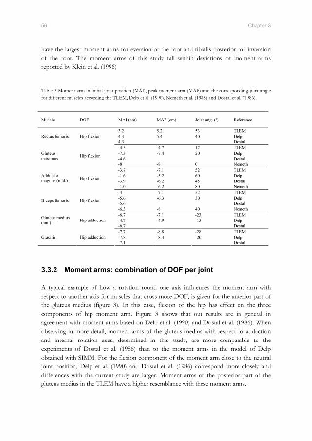
56 Chapter 3
have the largest moment arms for eversion of the foot and tibialis posterior for inversion of the foot. The moment arms of this study fall within deviations of moment arms reported by Klein et al. (1996) Table 2 Moment arm in initial joint position (MAI), peak moment arm (MAP) and the corresponding joint angle for different muscles according the TLEM, Delp et al. (1990), Nemeth et al. (1985) and Dostal et al. (1986).
3.3.2 Moment arms: combination of DOF per joint
A typical example of how a rotation round one axis influences the moment arm with respect to another axis for muscles that cross more DOF, is given for the anterior part of the gluteus medius (figure 3). In this case, flexion of the hip has effect on the three components of hip moment arm. Figure 3 shows that our results are in general in agreement with moment arms based on Delp et al. (1990) and Dostal et al. (1986). When observing in more detail, moment arms of the gluteus medius with respect to adduction and internal rotation axes, determined in this study, are more comparable to the experiments of Dostal et al. (1986) than to the moment arms in the model of Delp obtained with SIMM. For the flexion component of the moment arm close to the neutral joint position, Delp et al. (1990) and Dostal et al. (1986) correspond more closely and differences with the current study are larger. Moment arms of the posterior part of the gluteus medius in the TLEM have a higher resemblance with these moment arms.
Muscle DOF MAI (cm) MAP (cm) Joint ang. (º) Reference
3.2 5.2 53 TLEM 4.3 5.4 40 Delp Rectus femoris Hip flexion 4.3 Dostal -4.5 -4.7 17 TLEM -7.3 -7.4 20 Delp -4.6 Dostal
Gluteus maximus Hip flexion
-8 -8 0 Nemeth -3.7 -7.1 52 TLEM -1.6 -5.2 60 Delp -3.9 -6.2 45 Dostal
Adductor magnus (mid.) Hip flexion
-1.0 -6.2 80 Nemeth -4 -7.1 52 TLEM -5.6 -6.3 30 Delp -5.6 Dostal Biceps femoris Hip flexion
-6.3 -8 40 Nemeth -6.7 -7.1 -23 TLEM -4.7 -4.9 -15 Delp Gluteus medius
(ant.) Hip adduction -6.7 Dostal -7.7 -8.8 -28 TLEM -7.8 -8.4 -20 Delp Gracilis Hip adduction -7.1 Dostal
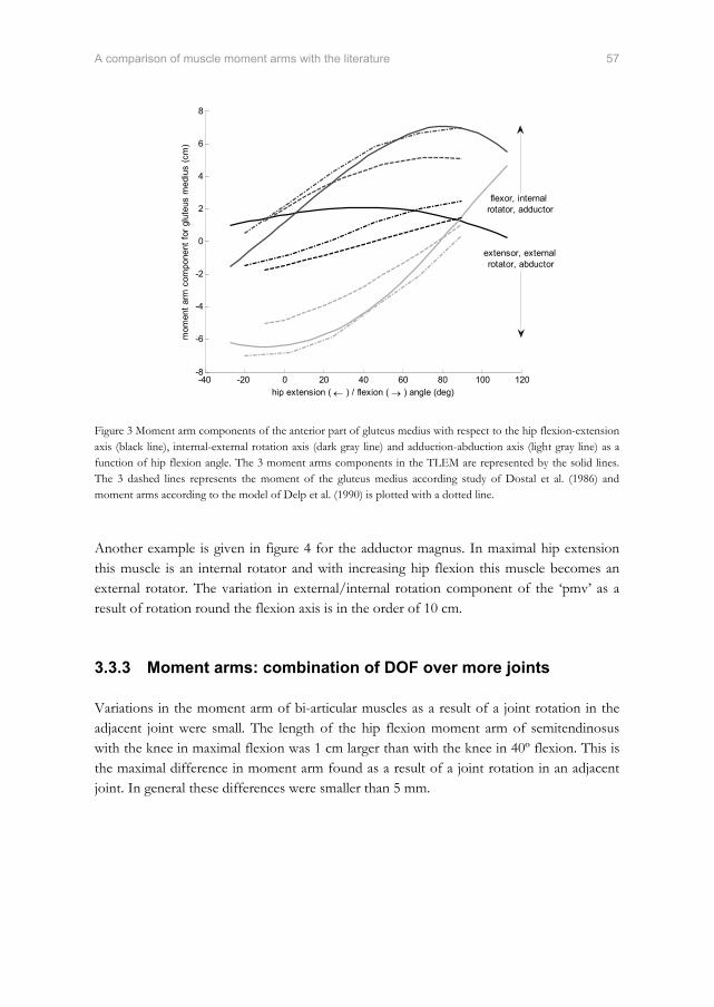
A comparison of muscle moment arms with the literature 57
-40 -20 0 20 40 60 80 100 120-8
-6
-4
-2
0
2
4
6
8
hip extension ( ← ) / flexion ( → ) angle (deg)
mom
ent a
rm c
ompo
nent
for g
lute
us m
ediu
s (c
m)
extensor, external rotator, abductor
flexor, internal rotator, adductor
Figure 3 Moment arm components of the anterior part of gluteus medius with respect to the hip flexion-extension axis (black line), internal-external rotation axis (dark gray line) and adduction-abduction axis (light gray line) as a function of hip flexion angle. The 3 moment arms components in the TLEM are represented by the solid lines. The 3 dashed lines represents the moment of the gluteus medius according study of Dostal et al. (1986) and moment arms according to the model of Delp et al. (1990) is plotted with a dotted line. Another example is given in figure 4 for the adductor magnus. In maximal hip extension this muscle is an internal rotator and with increasing hip flexion this muscle becomes an external rotator. The variation in external/internal rotation component of the ‘pmv’ as a result of rotation round the flexion axis is in the order of 10 cm.
3.3.3 Moment arms: combination of DOF over more joints
Variations in the moment arm of bi-articular muscles as a result of a joint rotation in the adjacent joint were small. The length of the hip flexion moment arm of semitendinosus with the knee in maximal flexion was 1 cm larger than with the knee in 40º flexion. This is the maximal difference in moment arm found as a result of a joint rotation in an adjacent joint. In general these differences were smaller than 5 mm.

58 Chapter 3
−10 −5 0 5 10−10
−8
−6
−4
−2
0
2
4
6
8
10
hip external ( ← ) / internal ( → ) rotation pmv component (cm)
hip
exte
nsio
n ( ←
) /
flexi
on (
→ )
pm
v co
mpo
nent
(cm
)
hip flexion angle = 93 deg.
hip flexion angle = 17 deg.
hip flexion angle = −3 deg.
hip flexion angle = −22 deg.
Figure 4 Projection of the potential moment vector of the adductor magnus in the transversal plane. Adductor magnus was divided in 3 muscle parts in the model based on differences in muscle architecture: proximal part described with 4 elements (triangle), middle part with 6 elements (cross) and a distal part with 3 elements (circle). Besides adduction, the adductor magnus contributes to hip internal rotation and extension for extreme hip extension angles and becomes an external rotator and flexor with increasing hip flexion.
3.4 Discussion
Accurate model moment arms are of major importance in acquiring meaningful model outputs (Erdemir et al., 2006). Moment arms play a direct role in the estimation of muscle force using a muscle load sharing criterion. The moment arm also influences the force-length and force-velocity characteristics of a muscle since it determines the relation between joint angle and the length of muscle (and between angular velocity and contraction velocity). A musculoskeletal model must be able to calculate the correct moment arms in any position. The purpose of this study was to compare calculated moment arms of the TLEM, a new musculoskeletal model of the lower extremity, with direct measurements and existing models from the literature. Since each measurement method has its own assumptions there is, unfortunately, no gold standard. However, a comparison of the model predictions with different measurement methods is useful, since all methods should produce results within a certain range. Moment arms acquired in earlier mentioned studies based on 2D imaging techniques and tendon excursion methods can only be compared to a 3D musculoskeletal model with limitations, since moment arms are not determined when more than one joint angle is varied. Nevertheless, a comparison could still be made by prescribing a rotation in the model around the concerned axis of the model to determine the moment arm in question.
A comparison of muscle moment arms with the literature 59
3.4.1 Inter-individual differences
Dissimilarity between muscle moment arms reported in this study and data from the literature are attributed to differences in morphology and differences in methods used. Anatomical variations in moment arm can be substantial. The reported range of peak moment arm of the patella tendon, measured in a cadaver study using a finite screw axis method, was 2 cm which is 50% of the lowest peak moment arm (Krevolin et al., 2004). In general, comparable inter-individual variations were found by Klein et al. (1996), although at some joint angles larger variations were reported (up to 5 cm for the triceps surae acting on the subtalar joint and up to 4 cm for tibialis anterior with respect to the talocrural joint).
3.4.2 Methodological differences
Variations in moment arm can only be fully attributed to different methods if the methods were applied to the same specimen. Spoor et al. (1992) compared moment arms obtained on the same specimen with MRI and tendon excursion and showed that moment arms can differ up to 1.1 cm as a result of the differences between methods. Since this study only comprises one specimen and two different methods, even larger variations might be possible. An advantage of the tendon excursion method is that the center of rotation and the application point of the moment arm at the tendon do not need to be explicitly determined (Spoor and van Leeuwen, 1992). Yet, unfortunately this method also has its limitations. The multiple joint angles which define the amplitude of the moment arm make it impractical to do these experiments for all muscles and combinations of degrees of freedom. Secondly, the muscles of the specimen are stiffened due to the embalming process, which hinders a joint rotation and subsequent measurement of the excursion of a tendon. All muscles fibers should therefore be cut and cleared away to allow free movement. This was impracticable in combination with the extensive cadaver measurements done by Klein Horsman et al. (2007). Finally, for muscles with broad attachment sites with fibers attaching directly to the bone (e.g. gluteus maximus), the accuracy of measurement of muscle excursion is disputable. A major drawback of the via point method based on 2D imaging techniques such as MRI is that the center of rotation is roughly estimated with a line between two bony landmarks, or a joint surface contact point. This line may differ significantly from the kinematic joint axis. Secondly, in case of broad muscle such as gluteus maximus the definition of a moment arm is less trivial than for example a muscle with a distinct tendon such as the Achilles tendon. This makes the calculated moment arm sensitive for artefacts and thus unreliable. Nevertheless MRI studies can be useful in understanding principles that influence moment arm (Maganaris et al., 1999). The moment arm of the triceps surae in plantar flexion in this study and an MRI study (Maganaris, 2001) differed more than 2 cm when compared to mean moment arm from the tendon excursion study of Klein et al. (1996). Maganaris (2001) measured moment arm at a maximal contraction level so that the muscle approaches a

60 Chapter 3
straight line as assumed in our model. However, in a tendon excursion experiment, surrounding tissues pull the non-activated muscle towards the tibia when a muscle is in plantar flexion, which reduces the moment arm in this region. This explains why our data have a better resemblance with the results of Maganaris (2001). A limitation in the representation of the muscle line of action in the origin-insertion method is the neglecting the effect of contraction level on the moment arm due to the thickness of the muscle, bulging of the muscle belly or stretch in the retinacula. Spoor et al. (1992) discussed the effect of contraction of the semimembranosus on the gastrocnemius moment arm and vice versa. In tibialis anterior for example the moment arm for talocrural flexion can increase with 1.5 cm with maximal contraction (Maganaris et al., 1999). An anatomically realistic implementation of these effects in a comprehensive musculoskeletal model was not found in the literature.
3.4.3 Evaluation of the validity of the model
In general the moment arms of the TLEM fall within the range of moment arms determined for other subjects (Klein et al., 1996), which is a minimum condition to declare the results trustworthy. A comparison with moment arms based on a single dataset, as with the model of Delp et al. (1990), is hampered since differences due to inter-individual variation are unknown. It is assumed that differences smaller than 2 cm can be attributed to inter-individual variation. Larger variations were attributed to differences in methodology. Differences larger than 2 cm were not only observed between the TLEM and the literature, but also between different studies in the literature. Muscle moment arm in initial joint position in two studies (Dostal et al., 1986, Nemeth and Ohlsen, 1985) based on an origin-insertion method but with a different method to define attachment sites, differed 3 cm (table 2). Besides inter-individual differences, a cause for such a variation is a methodological difference in representing a muscle with a broad attachment site by a limited number of muscle elements. The moment arm of the current study has a good resemblance with the data from Dostal et al. (1986). The current study is the first step in the evaluation of the validity of the TLEM. By including the force generating properties that were measured on the same subject, several other measures such as maximal joint torques could be determined and compared with literature or experimental data to further improve the reliability of model outputs.
3.4.4 Strengths and limitations of the model
The presented model is based on an accurate and extensive anatomical dataset of the lower extremity containing all the required data for the construction of a large scale musculoskeletal model. Accurate measurement of joint parameters, muscle attachment sites and intervening
A comparison of muscle moment arms with the literature 61
structures resulted in an extensive representation of the mechanical effect of the muscles in the model. Muscles are defined with a sufficient number of muscle elements (Van der Helm and Veenbaas, 1991) that are able to curve around geometric shapes or through via points if intervening structures such as bony contours or retinacula were present. For an accurate representation of the force-length characteristics of a muscle a subdivision in elements with different moment arms is important, since the length change of each element as a result of a joint rotation is different. In comparison to Brand et al. (1982) and Delp et al. (1990) and many other models based on this dataset, the mechanical effect of the muscles is more extensively represented in the TLEM (e.g. figure 2). Besides parameters that define the muscle moment arm, other relevant muscle architectural properties such as PCSA, optimal fiber length and tendon length were assigned to the muscle elements, which are needed for muscle force estimation. Where other comprehensive models such as Delp et al. (1990) merge different datasets and estimate missing parameters to construct a model, this model is based on one cadaver, which is a major advantage since co-variances between parameters such as moment arm and fiber length are maintained. Collecting all model parameters on a subject to develop a subject specific model is a challenge in musculoskeletal modelling. The use of a generic (cq. this) model for patient-specific evaluations of clinical applications has its limitations, since ideally subject specific model parameters are used for this purpose. With MRI or other imaging technique subject specific parameters can be collected, but only to a limited extent. The use of via points through a stack of 2D images is only valid in the one measured position, but will cause errors when extrapolated to other positions, e.g. during axial rotations via points will not adequately present the muscle line of action anymore. Only the origin-insertion method will allow for calculations of the moment arms in any position of the model. Important muscle parameters for muscle force estimation such as optimal fiber length cannot be determined using imaging techniques. Another drawback of MRI is the difficulty to recognise the attachment sites on the bone, which makes a calculated muscle line of action questionable. It is likely that scaling of the generic dataset will improve the resemblance with the subject’s anatomy. Yet, scaling is only effective if a correlation between the anatomical parameters and the scaling parameters has been shown. One MRI study was reported showing good correlation between moment arms and external measures (Murray et al., 2002). Until now, no such studies based on accurate measurements on multiple specimens have been published. Scaling parameters are currently based on non-validated assumptions. On the way towards the development of subject specific models the collection of more consistent and comprehensive anatomical datasets on a large number of specimens would be very relevant. This would require a major effort of many research groups all using the same measurement protocol, in order to obtain a well-validated ‘industrial standard’. These data can be used to develop accurate and extensive scaling regression equations based on externally measurable subject dimensions which would improve the resemblance of the model with the anatomy of the subject. This will be one of the future challenges in musculoskeletal modelling, which has probably a long way to go. In the meantime this model will be of great value.

62 Chapter 3
3.5 References
An, K. N., Takahashi, K., Harrigan, T. P.,Chao, E. Y., 1984. Determination of muscle orientations and moment arms. Journal of Biomechanical Engineering, 106, 280-2.
Anderson, F. C.,Pandy, M. G., 1999. A Dynamic Optimization Solution for Vertical Jumping in Three Dimensions. Computer Methods Biomechanics and Biomedical Engineering, 2, 201-231.
Arnold, A. S., Blemker, S. S.,Delp, S. L., 2001. Evaluation of a deformable musculoskeletal model for estimating muscle-tendon lengths during crouch gait. Annals of Biomedical Engineering, 29, 263-74.
Boone, D. C.,Azen, S. P., 1979. Normal range of motion of joints in male subjects. Journal of Bone and Joint Surgery, 61, 756-9.
Brand, R. A., R.D., C., Wittstock, C. E., Pedersen, D. R., Clark, C. R.,Van Krieken, F. M., 1982. A model of the lower extremity muscular anatomy. Journal of Biomechanical Engineering, 104, 304-310.
Delp, S. L.,Loan, J. P., 1995. A graphics-based software system to develop and analyze models of musculoskeletal structures. Computers in Biology and Medicine, 25, 21-34.
Delp, S. L., Loan, J. P., Hoy, M. G., Zajac, F. E., Topp, E. L.,Rosen, J. M., 1990. An interactive graphics-based model of the lower extremity to study orthopaedic surgical procedures. IEEE Transactions on Biomedical Engineering, 37, 757-67.
Dostal, W. F., Soderberg, G. L.,Andrews, J. G., 1986. Actions of hip muscles. Physical Therapy, 66, 351-61.
Erdemir, A., Mclean, S., Herzog, W.,Van Den Bogert, A. J., 2006. Model-based estimation of muscle forces exerted during movements. Clinical Biomechanics (Bristol, Avon).
Fick, A. E.,Weber, E., 1877. Anatomisch-mechanische Studie ueber die Schultermuskeln I. Verhandl. Würz. Phys. Med. Ges., 11, 123-153.
Fukunaga, T., Ito, M., Ichinose, Y., Kuno, S., Kawakami, Y.,Fukashiro, S., 1996. Tendinous movement of a human muscle during voluntary contractions determined by real-time ultrasonography. Journal of Applied Physiology, 81, 1430-3.
Gregor, R. J., Komi, P. V., Browning, R. C.,Jarvinen, M., 1991. A comparison of the triceps surae and residual muscle moments at the ankle during cycling. Journal of Biomechanics, 24, 287-97.
Grieve, D. W., Pheasant, S.,Cavanagh, P. R. 1978 Prediction of gastrocnemius length from knee and ankle joint posture, Baltimore, MD, University Park Press.
Higginson, J. S., Zajac, F. E., Neptune, R. R., Kautz, S. A., Burgar, C. G.,Delp, S. L., 2006. Effect of equinus foot placement and intrinsic muscle response on knee extension during stance. Gait and Posture, 23, 32-6.
Hogfors, C., Sigholm, G.,Herberts, P., 1987. Biomechanical model of the human shoulder--I. Elements. Journal of Biomechanics, 20, 157-66.
Jensen, R. H.,Davy, D. T., 1975. An investigation of muscle lines of action about the hip: a centroid line approach vs the straight line approach. Journal of Biomechanics, 8, 103-10.
Klein Horsman, M. D., Koopman, H. F., Van Der Helm, F. C., Prose, L. P.,Veeger, H. E., 2007. Morphological muscle and joint parameters for musculoskeletal modelling of the lower extremity. Clinical Biomechanics (Bristol, Avon), 22, 239-47.

A comparison of muscle moment arms with the literature 63
Klein, P., Mattys, S.,Rooze, M., 1996. Moment arm length variations of selected muscles acting on talocrural and subtalar joints during movement: an in vitro study. Journal of Biomechanics, 29, 21-30.
Koolstra, J. H., Van Eijden, T. M., Van Spronsen, P. H., Weijs, W. A.,Valk, J., 1990. Computer-assisted estimation of lines of action of human masticatory muscles reconstructed in vivo by means of magnetic resonance imaging of parallel sections. Archives of Oral Biology, 35, 549-56.
Krevolin, J. L., Pandy, M. G.,Pearce, J. C., 2004. Moment arm of the patellar tendon in the human knee. Journal of Biomechanics, 37, 785-8.
Maganaris, C. N., 2001. Force-length characteristics of in vivo human skeletal muscle. Acta Physiologica Scandinavica, 172, 279-85.
Maganaris, C. N., Baltzopoulos, V.,Sargeant, A. J., 1999. Changes in the tibialis anterior tendon moment arm from rest to maximum isometric dorsiflexion: in vivo observations in man. Clin Biomech (Bristol, Avon), 14, 661-6.
Maganaris, C. N., Baltzopoulos, V.,Sargeant, A. J., 2000. In vivo measurement-based estimations of the human Achilles tendon moment arm. European Journal of Applied Physiology and Occupational Physiology, 83, 363-9.
Mollier, S., 1899. Ueber die Statik und Mechanik des Menslichen Schultergurtels unter Normalen und Pathologischen Verhaltnissen. Festschr. f. C. v. Kupffer, Jena.
Murray, W. M., Buchanan, T. S.,Delp, S. L., 2002. Scaling of peak moment arms of elbow muscles with upper extremity bone dimensions. Journal of Biomechanics, 35, 19-26.
Nemeth, G.,Ohlsen, H., 1985. In vivo moment arm lengths for hip extensor muscles at different angles of hip flexion. Journal of Biomechanics, 18, 129-40.
Neptune, R. R., Zajac, F. E.,Kautz, S. A., 2004. Muscle force redistributes segmental power for body progression during walking. Gait and Posture, 19, 194-205.
Pierrynowski, M. R., 1995. Analytic representation of muscle line of action and geometry, in: Allard, P., Stokes, I. A. F. & Blanchi, J. P. (Eds.) Three-Dimensional Analysis of Human Movement. Human Kinetics, Champaign, IL, pp. 214-256.
Spoor, C. W.,Van Leeuwen, J. L., 1992. Knee muscle moment arms from MRI and from tendon travel. Journal of Biomechanics, 25, 201-6.
Van Der Helm, F. C., 1994. A finite element musculoskeletal model of the shoulder mechanism. Journal of Biomechanics, 27, 551-69.
Van Der Helm, F. C., Veeger, H. E., Pronk, G. M., Van Der Woude, L. H.,Rozendal, R. H., 1992. Geometry parameters for musculoskeletal modelling of the shoulder system. Journal of Biomechanics, 25, 129-44.
Van Der Helm, F. C.,Veenbaas, R., 1991. Modelling the mechanical effect of muscles with large attachment sites: application to the shoulder mechanism. Journal of Biomechanics, 24, 1151-63.
Veeger, H. E. J.,Van Der Helm, F. C., 2006. Shoulder Function: the perfect compromise between mobility and stability. Journal of Biomechanics [submitted].
Visser, J. J., Hoogkamer, J. E., Bobbert, M. F.,Huijing, P. A., 1990. Length and moment arm of human leg muscles as a function of knee and hip-joint angles. European Journal of Applied Physiology and Occupational Physiology, 61, 453-60.
Wu, G., Siegler, S., Allard, P., Kirtley, C., Leardini, A., Rosenbaum, D., Whittle, M., D'lima, D. D., Cristofolini, L., Witte, H., Schmid, O.,Stokes, I., 2002. ISB recommendation on definitions of joint coordinate system of various joints for the reporting of human joint motion--part I: ankle, hip, and spine. International Society of Biomechanics. Journal of Biomechanics, 35, 543-8.


Chapter 4
The Twente Lower Extremity Model: a comparison of
maximal isometric moment with the literature
M.D. Klein Horsman, H.F.J.M. Koopman, H.E.J. Veeger and F.C.T. van der Helm Submitted to Journal of Biomechanics, 2007
Abstract
Accuracy of comprehensive musculoskeletal models is highly dependent on consistency of its parameters. Since a complete dataset is as yet not available, these models have been constructed using different datasets. We developed a musculoskeletal model of the lower extremity based on a recently collected, complete and consistent anatomical dataset. The aim of this study is the evaluation of the validity of the model by comparing maximal isometric joint moments simulated with the model with in vivo measured maximal voluntary moments from the literature. Maximal isometric moments are determined with respect to 6 joint axes of the model based on full activation of all corresponding Hill-type muscle elements in the model. Maximal isometric moments correspond with in vivo measured maximal voluntary moments, except for knee extension and plantar flexion where a large difference was found in angle at which peak moment occurred. In other comprehensive musculoskeletal models different datasets are merged and missing parameters estimated such that a good fit is obtained. This may be functional but will not necessarily result in an accurate representation. The added value of the current model is that all parameters are based on the same specimen so that different parameters are consistent. Deviations found for knee extensors and plantar flexors showed limitations in representation of these muscles using a Hill model. Adaptation of measured tendon length led to a good fit with in vivo data.

A comparison of maximal isometric moments with the literature 67
4.1 Introduction
Comprehensive musculoskeletal models are needed to get more insight how muscle force and joint moment are affected by orthopedic interventions in the geometry of the musculoskeletal system (Delp et al., 1990, Arnold et al., 2001). Simulating the kinematic and dynamic behaviour of the musculoskeletal system will give insight in how muscle force is produced and the resulting movement is controlled. The study presented here is part of a larger project that aims to develop an inverse and forward 3D musculoskeletal model of the lower extremity to assist in the treatment of gait disorders by the evaluation of if-then scenarios. The outcome of a musculoskeletal model is highly dependent on its geometry, specified by anatomical parameters. Joint and muscle geometry define the moment arms and length of a muscle. Combined with muscle parameters such as optimal fiber length and physiological cross sectional area (PCSA), the maximal force and moment generated by a muscle can be estimated. Various anatomical datasets of the lower extremity have been reported in the literature, containing model parameters such as muscle attachment sites (Pierrynowski, 1995, Brand and Crowinshield, 1982) or muscle force generating properties like optimal fiber length and PCSA (Wickiewicz et al., 1983, Spoor et al., 1991, Weber, 1851). However, a dataset containing all the required model parameters obtained from one specimen was not available. Therefore, when constructing a comprehensive musculoskeletal model different datasets had to be merged and missing parameters estimated to obtain the required complete dataset. By combining the anatomical properties from different specimens the possible effect of inter-individual differences, or intra-individual ‘tuning’ is not taken into account. We have developed a musculoskeletal model of the lower extremity (Klein Horsman et al., 2007b) in which all model parameters were based on a recently collected extensive anatomical dataset (Klein Horsman et al., 2007a). The goal of this study is to evaluate the validity of this model by comparing maximal isometric joint moments, simulated with the model, with in vivo measured maximal voluntary moments from the literature.
68 Chapter 4
4.2 Methods
4.2.1 Twente Lower Extremity Model
The Twente lower extremity model (TLEM) is a recently developed comprehensive musculoskeletal model of the lower extremity in which an extensive set of connected elements are defined, each representing a relevant morphological structure of the lower extremity (Klein Horsman et al., 2007b). All the parameters assigned to the elements are based on a recently measured anatomical dataset on a right lower extremity (Klein Horsman et al., 2007a). The model has 21 degrees of freedom (DOF). The left and right hip are modelled as a ball socket joint (each 3 DOF); the knee, ankle and subtalar joint are defined as single hinge joints (each 1 DOF). The other DOF, which fall outside the scope of this study, describe the position and orientation of the pelvis in 3D (6 DOF) and the orientation of the trunk (3 DOF). By prescribing these generalised coordinates, kinematic properties of the elements in the model, such as muscle elements, can be determined. The model contains 264 muscle elements to describe the mechanical effect of 76 muscles of both the lower extremities. A muscle element is defined by the position of origin and insertion. In case of curvature due to intervening structures, ‘via’ points and geometric shapes are used to describe the muscle line of action more accurately. Each muscle element is considered to be an independent actuator with its own set of muscle parameters (muscle mass, pennation angle, physiological cross-sectional area (PCSA), tendon length and optimal fiber length). More details about the structure of the TLEM and the resulting moment arms are described in a previous study (Klein Horsman et al., 2007b).
4.2.2 Maximal isometric moment
The maximal isometric muscle force was calculated for the active range of motion of the joints (Boone and Azen, 1979) using the muscle parameters assigned to the muscle element. A muscle was modelled as a standard Hill-type muscle element as shown in figure 1 (Winters and Stark, 1985). The length of a musculotendon complex Lmus was defined as the length of the muscle element, calculated as the distance between the origin and insertion on both body segments. For a curved muscle element, the length was defined as the shortest distance between origin and insertion around the surface of a geometric shape. In case of a via point, muscle length was defined as the length of the muscle element plus a constant length between the real attachment and the pseudo attachment.

A comparison of maximal isometric moments with the literature 69
Lt Lse
d0
L ce
PE
SE
CE
Lmus
α
Figure 1 Hill model with contractile element (CE), series elastic element (SE) and parallel elastic element (PE). d0 is assumed to be constant, hence Lce and α can be calculated for a given Lmus, Lt and Lse. The width d0 of the muscle due to pennation was assumed constant, based on the assumption of a constant muscle volume during contraction (van Der Linden et al., 1998). d0 was calculated with the initial pennation angle α0 and initial length of the contractile element Lce0 (figure1):
000 *)sin( ceLd α= (1) The actual pennation angle α can be calculated using actual fiber length:
)arctan( 0
setmus LLLd
−−=α
(2) The length of contractile element Lce was determined with the length of the tendon Lt and the lengthening of the series-elastic element Lse, assumed to be zero in the first approach.
)cos(αsetmus
ceLLLL −−
= (3)
The normalised force length relation was described with a Gaussian relation:
⎟⎟
⎠
⎞
⎜⎜
⎝
⎛⎟⎟⎠
⎞⎜⎜⎝
⎛ −−=
2
0exp)(cesh
cece
LLLlf
(4)

70 Chapter 4
Lcesh, defined as 0.5*Lce0, is a shape parameter determining the width of the f-l curve. With these parameters the maximal isometric force Fce in the contractile element was calculated as a function of joint angle:
max)cos()()( FvflfaFce ⋅⋅⋅⋅= α (5) In which Fmax is the maximal muscle force:
maxmax *σPCSAF = (6) For the simulation of maximal isometric moment, muscle activation a and force-velocity properties f(v), normally varying between 0 and 1, were set to 1. In this study we used a maximal stress in a muscle fiber σmax of 27 N/cm2 which falls in the range of values reported in the literature (Spector et al., 1980, Powell et al., 1984, Weijs and Hillen, 1985). Passive forces in the parallel elastic element, representing resistance forces of passive structures such as the epimysium and perimysium, were described as a function of the Lmus:
)1(1
max −−
=⋅
−
PExmPEsh
lPEshpe
muso
musolmusl
ee
FF (7)
In which lmuso is the length of the muscle at optimum fiber length. Parameters PEsh and PExm, describing the shape of the curve, were set to respectively 4 and 0.4 (Winters and Stark, 1988). The total muscle force was defined as:
pecemus FFF += (8)
Finally the maximal isometric moment Mmus was computed by multiplying Fmus with the moment arm d:
musmus FdM ×= (9) The maximal isometric joint moment was determined by a summation of the contributing muscle elements:
∑=n
musMM max (10)

A comparison of maximal isometric moments with the literature 71
4.2.3 TLEM in comparison with in vivo data and Delp et al. (1990)
The maximal isometric joint moments of the hip, knee and ankle were determined with and without the passive component as a function of the corresponding joint angle. Joint angle is defined with respect to the initial model position in which the local pelvis coordinate system is aligned with the global reference frame and all joints are in a neutral position as described by Klein Horsman et al. (2006b). In order to evaluate the validity of the model a comparison is made with in vivo measured maximal voluntary joint moments from the literature. In the simulations all relevant joint angles were equalised with the angles in the in vivo measurements. The following curve properties were compared: the shape, the angle of peak moment and the amplitude. A specific tension of 27 N/cm2 was used to scale the strength of the model with in vivo data. Secondly, a comparison is made with maximal isometric joint moments based on the frequently used public domain biomechanical model of Delp et al. (1990). These moments were simulated with SIMM (Delp and Loan, 1995, Delp et al., 1990).
4.3 Results
The maximal isometric hip flexion moment determined with the TLEM shows small deviations (<30 Nm) with respect to the moments based on the model of Delp et al. (1990) (figure 2). The moment curve falls within the 95% confidence interval (CI) of the maximal voluntary moment measured by Inman et al. (1981), except for the small CI (12 Nm) at 40º hip flexion. Yet, at 45º hip flexion the simulated moment falls within the CI of the flexion moment measured by Cahalan et al. (1989). The flexion moment at 10º hip flexion determined with the TLEM and Delp’s model falls outside the CI of the moment reported by Cahalan et al. (1989) and is around 80 Nm smaller. The maximal isometric hip extension moment falls within the CI of the different studies (Waters et al., 1974, Nemeth and Ohlsen, 1985, Cahalan et al., 1989). In vivo studies show an increase in joint extension moment with an increase of flexion angle. However, in our simulations between 45º and 75º a small decrease of 38 Nm is observed. Moments determined with the model of Delp show a decrease of 120 Nm from 40º to 120º hip flexion. In comparison to other joint axes, a relatively large contribution of passive forces can be observed for hip extension (up to 33% of total moment at maximal flexion), which is in agreement with in vivo measured passive forces (Yoon and Mansour, 1982). Hip internal and external rotation moments simulated with the TLEM fall within the CI of the moments measured by Cahalan et al. (1989). The same counts for moments simulated with Delp’s model. More in vivo data with respect to this joint axis are lacking in the literature.

72 Chapter 4
-40 -20 0 20 40 60 80 100 120-400
-300
-200
-100
0
100
200
300
hip extension ( ← ) / flexion ( → ) angle (deg)
hip
exte
nsio
n ( ←
) / f
lexi
on ( →
) m
omen
t (N
m)
-50 -40 -30 -20 -10 0 10 20 30 40 50-150
-100
-50
0
50
100
150
hip external ( ← ) / internal ( → ) rotation angle (deg)
hip
exte
rnal
( ←
) / i
nter
nal (
→ )
rota
tion
mom
ent (
Nm
)
-50 -40 -30 -20 -10 0 10 20 30 40-300
-200
-100
0
100
200
300
hip abduction ( ← ) / adduction ( → ) angle (deg)
hip
abdu
ctio
n ( ←
) / a
dduc
tion
( → )
mom
ent (
Nm
)
-120 -100 -80 -60 -40 -20 0 20-200
-100
0
100
200
300
400
500
knee flexion ( ← ) / extension ( → ) angle (deg)
knee
flex
ion
( ← )
/ ext
ensi
on ( →
) m
omen
t (N
m)
-60 -50 -40 -30 -20 -10 0 10 20 30 40-500
-400
-300
-200
-100
0
100
plantar flexion ( ← ) / dorsal flexion ( → ) angle (deg)
plan
tar f
lexi
on ( ←
) / d
orsa
l fle
xion
( →
) m
omen
t (N
m)
Waters et al. (1974), 8 wNemeth et al. (1983), 10 m&wCahalan et al.(1989), 17 mInman et al. (1981), 3 mOlsen et al. (1972), 30 mJohnson et al. (2004), 38 wMurray et al. (1968), 20 mArokoski et al. (2002), 30 mMurray et al.(1977), 24 mInman et al. (1981) 4 ...Pincivero et al. (2004), 14 mWelsch et al. (1998), 77 m&wSale et al. (1982), 20 mMaganaris (2003), 8 mMarsh et al. (1981), 25 mMiyamoto et al.(2003), 8 mFukanaga et al. (1996), 8 mDelp et al. (1990)TLEM active + passiveTLEM activeTLEM uncorrected
Figure 2 Maximal isometric moments with respect to generalized coordinates of the model in comparison with in vivo studies and Delp et al. (1990). The solid line shows the sum of active and passive component, the dotted line shows the contribution of the active muscles only. The non varying joints were in initial joint position as in the in vivo studies. Except for internal and external rotation, moments were determined in 60º hip flexion and 90º flexion as in the study of Cahalan et al. (1969). For knee extension the hip was flexed 90 degrees as in the seating position in the in vivo studies. ‘TLEM uncorrected’ represents the knee extension and plantar flexion moment without adaptation in patella and achilles tendon length. For in vivo values the 95% confidence interval (2 times SD) is plotted. Number of subjects and the gender (m/w) is mentioned in the legend.

A comparison of maximal isometric moments with the literature 73
As for the model of Delp, simulated hip adduction moment fall outside the CI of some studies (Cahalan et al., 1989, Johnson et al., 2004), but resemble well with other studies (Murray and Sepic, 1968, Arokoski et al., 2002). In agreement with in vivo measurements (Olson et al., 1972, Cahalan et al., 1989, Murray and Sepic, 1968), the simulated hip abduction curve shows an increase in moment from 50º to 5º abduction. But in contrast to Delp’s model, the values fall outside the CI. The literature is ambiguous about this amplitude. The joint moment determined with the TLEM falls within the CI of the joint moments reported by Arokoksi et al. (2002) and Johnson et al. (2004); the latter reported normalized moments which were scaled to the dimensions of the specimen in the current study. From -5º to 20º adduction our results show a decrease in moment which is not observed in the in vivo studies and only to a limited extend in moments determined with Delp’s model. For knee extension and plantar flexion a large deviation of angle of peak moment was found with respect to the unambiguous data from the literature. By lengthening the patella and Achilles tendon with 5 cm a reasonable fit was obtained. In vivo measured knee extension moment peaks at 60º, where the moment based on our simulations peaks at 10º before and 55º after correction; the moment based on Delp’s model peaks at 30º. The shape of the corrected moment curve resembles well with the data reported in the literature (Murray et al., 1977, Pincivero et al., 2004, Welsch et al., 1998). In most cases the amplitude of the knee extension moment falls in the lower regions of CI of the different studies. The effect of the lengthening of the tendon of rectus femoris on the hip joint moment was minimal, therefore only the corrected moments are plotted in figure 2. Just as for the model of Delp, the simulated knee flexion moment corresponds reasonably well with the range of in vivo measured moments, although at knee angles between 30º and 60º the slight decrease of knee flexion moment (Inman et al., 1981, Welsch et al., 1998, Murray et al., 1977) was not observed in the simulated moment. The lengthening of the Achilles tendon resulted in a shift to the right of peak knee flexion moment. Figure 2 shows the corrected plot. The inter-individual differences in dorsal flexion moments reported in the literature were small (CI < 6 Nm) (Fukunaga et al., 1996, Marsh et al., 1981). The shape of the simulated dorsal flexion moment curve is comparable with the study from Fukunaga et al. (1996). However the amplitude is around 2 times lower and more in agreement with the study of Marsh et al. (1981). The shape of the corrected plantar flexion moment curve is comparable with the in vivo studies (Maganaris, 2003, Sale et al., 1982, Miyamoto and Oda, 2003, Fukunaga et al., 1996) The moment curve peaks around 10º dorsal flexion, which corresponds with the joint moment curve measured by Maganaris et al. (2003) and Sale et al. (1982) and the simulated moment based on Delp’s model. A study reporting measurements of maximal isometric moments for subtalar inversion and eversion was not found in the literature, so a comparison could not be made.
74 Chapter 4
4.4 Discussion
The goal of this study was to evaluate the validity of the force generating properties of the TLEM, a comprehensive musculoskeletal model presented by Klein Horsman et al. (2007b). It was impossible to measure the actual maximal isometric moments on the specimen on which this model is based (Klein Horsman et al., 2007a). Therefore the accuracy of the model is evaluated by comparing simulated maximal isometric moments with maximal voluntary torque measurements from the literature. For a functional and reliable model it is essential that simulated moments reasonably correspond with in vivo measured moments. Unrealistic large deviations caused by inaccuracies in the representation of the mechanical effect of the muscles will lead to errors when the model is further utilized. For example, inaccurate determination of maximal muscle force results in inaccurate constraints for an optimization criterion in order to solve the load sharing problem. This will subsequently lead to an unreliable estimation of muscle force.
4.4.1 Comparison with maximal voluntary moment
The simulated moment curves are compared with maximal voluntary moment curves from the literature based on shape, angle of peak moment and amplitude. Unfortunately, there are three causes that partly hindered the evaluation of the validity of the model based on this comparison. The first is absence or limitedness of data. A comparison with in vivo subtalar inversion moments could not be made since these data are lacking in literature. Arokoski et al. (2002), Cahalan et al. (1989), Johnson et al. (2004) and Murray et al. (1968) report only one or two data points, which is insufficient to make a comparison of the shape of the curve. The second cause is that for some joint moments the literature is ambiguous. A clear example is the amplitude of adduction moment reported for men (age 40-81 years) in neutral position by Cahalan et al. (1989) which is two times smaller than the moment reported by Murray et al. (1968) (men, age 40-55 years). These deviations are caused by inter-individual variations and differences in methodology. The first group measured moments in a standing position in a frame with handles for body stabilizing, the second in a prone position during bilateral contractions. For the given example it is not possible to consider one study 100% reliable in comparison to the other since both studies can be considered reliable despite their limitations. Other studies show small variations (e.g. for knee extension), which enables an evaluation of the model validity. If the curve falls within the 95% CI of the different studies the model output is considered trustworthy. The third cause that hindered the validation is the unknown level of activation and specific tension in the in vivo experiments. Due to neurological limitations, limited motivation or in order to reduce unwanted joint moments of muscles that span multiple joint axes, a maximal
A comparison of maximal isometric moments with the literature 75
voluntary contraction does not correspond with a full excitation of all motor units (Enoka, 1988). Several studies report activation levels, roughly varying from 85 to 95% (see for overview (de Ruiter et al., 2004)). Nonetheless, the exact level in the experiments remains uncertain and might even be lower, for example due to limited training. Specific tension is used in musculoskeletal models to scale its strength in order to fit in vivo data. In Delp’s model a high specific tension of 61 N/cm2 was required, which falls outside the wide range reported in the literature (15 – 47 N/m2 according overview of Fukunaga et al. (1996)). This indicates that this model is based on atrophied specimens. The specific tension of 27 N/cm2 used in the TLEM falls within this range. This value is relatively low which is in agreement with the relatively high muscle mass observed in the specimen (Klein Horsman et al., 2007a). However, since different, on itself reliable, studies report ambiguous values, a validation of the amplitude of moment curve is hampered. Despite the three causes mentioned above, for some joints sufficient data are reported which are in mutual agreement so that the validity of the model could be evaluated by comparison of shape and angle of peak moment. For example the hip extension moment increases with increase of hip flexion angle in the three studies, which is in agreement with the moment simulated with the TLEM. The results showed that in most cases simulated joint moments fall within the total range of the different studies, which makes the model and its parameters more reliable. However, the comparison also showed limitation of the model. Unrealistic large deviations in angle of peak moment were found for knee extension and plantar flexion (see uncorrected curve in figure 2). There are a number of possible explanations. First is a change in anatomical configuration after fixation. The joint angles at death might have been different than the joint angles as measured after fixation. For example if the knee was more flexed at death, a stretch out in tendons might have caused a change in joint angle. In this case the measured sarcomere length corresponds to a different joint angle which would explain the shift of peak moment. Secondly, the assumption was made that the muscles were fully stretched and form a straight line when measured in the reference specimen position. However, this is only approached when muscles are in maximal contraction, which was not the case. For example the muscle belly of the triceps surae was loose and the Achilles tendon arched towards the ankle as a result of the surrounding tissue. Therefore the foot can be lifted until the muscle is stretched as assumed in the model. This shifts curve to the right. Thirdly, the flexion between the talus and calcaneus was neglected in the model. This results in an overestimation of the deformation in the soleus muscle element as in reality for a given ankle flexion angle insertion comes closer to the origin due to flexion between the talus and calcaneus. Relative dorsiflexion angles of 5º (SD 4º) were reported between these segments during stance phase (Hamel et al., 2004). The fourth effect not taken into account is the heterogeneity of sarcomere length. In rat semimembranosus muscle this effect augmented the length range of the left flank of the f-l curve with 38 to 43% (Willems and Huijing, 1994). It is plausible that with more detailed study, sarcomere distributions can be observed that will influence the width of the force length curve and will lead to a shift of the peak moment.

76 Chapter 4
Finally, by reducing the complex 3D construction of muscle to a 1D Hill-type model muscle, muscle deformation is described in a limited extend. For example, a possible lengthening of fibers at the surface of a muscle belly as a result of the bulging the muscle belly in contraction, is not accounted for. By lengthening both tendons with 5 cm the joint peak moment is shifted resulting in a reasonable fit with in vivo data. These adaptations are recommended when using the anatomical dataset of Klein Horsman et al. (2007a) in a 1D Hill-model (2007).
4.4.2 Comparison with Delp et al. (1990)
Although some differences can be observed in figure 2, for example for plantar flexion, in general our simulations correspond well with curves generated with the public domain model based on the work of Delp et al. (1990). However, similar simulated moments does not necessary stand for equal contributions of the muscles, which can be seen in figure 3.
0
5
10
15
20
25
TensorFascia Latae
AdductorLongus
AdductorBrevis
Sartorius Psoas Major
Hip
flex
ion
mom
ent a
t 0 d
egre
es h
ip fl
exio
n (N
m) TLEM
Delp et al. (1990)
Figure 3 Contribution of a selection of hip-flexor muscles to maximal isometric hip flexion moment at 0º of hip flexion in TLEM and model of Delp (1990).
This typical example shows that, although isometric moment at 0º hip flexion are equal, differences in contributions of muscles can be eminent. These variations are mainly a result of a sequence of in itself acceptable inter-individual variations in model parameters used to determine the maximal isometric moment (e.g. PCSA, optimal fiber length, pennation angle, moment arm). However, in Delp’s model, datasets are merged or missing data estimated in order to fit in vivo data. The resulting model describes an anatomical configuration that never existed. Since all parameters form a coherent and functional whole, possible subject-specific relations such as the moment arm to fiber length ratio are lost, which is a disadvantage in

A comparison of maximal isometric moments with the literature 77
comparison to the TLEM. For example, in Delp’s model, optimal fiber lengths are based on 2 anatomical datasets (Wickiewicz et al., 1983, Friederich and Brand, 1990). Wickiewicz et al. (1983) reported the number of sarcomeres in the fibers, but the corresponding joint angles were not accurately defined. Friederich and Brand (1990) only measured the length of the fiber. Therefore the angle at which a fiber is at optimal length had to be guessed. In this study the moment arm, the deformation of a muscle element and thus the fiber length change is determined for a given change in joint angle. Klein Horsman et al. (2007a) measured mean sarcomere length of a specimen together with the joint angles, so that in the corresponding model position the sarcomere length is known. With the measured fiber length, the number of sarcomeres in series is determined and thus the force-length properties of the muscle fiber as a function of joint angle. For plantar flexion and knee extension moment this approach resulted in large deviations with respect to in vivo data showing a limitation of the Hill-type muscle model. Such limitations are concealed when one can select the most appropriate parameters from different specimens or guess parameters that suit the best to end up with a functional model. For example by selecting the longest muscle fiber and smallest moment arm from the available datasets the desirable wide range of active muscle force might be obtained. The resulting model may be functional but not necessary an accurate representation.
4.4.3 Concluding remarks
In this study anatomical parameters, collected on one subject, are implemented in a model to determine maximal isometric moment. The simulations led in most cases to a reasonable fit with maximal voluntary torque measurements from the literature, which makes this model suitable for further inverse and forward dynamic analysis. This result is unique since the model is based on one consistent dataset. The direct implementation of anatomical parameters in this study also showed a shortcoming in the representation of plantar flexors and knee extensors using a Hill model. Possible causes are described and with a relatively easy solution it is shown that a reasonable fit can be obtained.
4.5 References
Arnold, A. S., Blemker, S. S.,Delp, S. L., 2001. Evaluation of a deformable musculoskeletal model for estimating muscle-tendon lengths during crouch gait. Annals of Biomedical Engineering, 29, 263-74.
Arokoski, M. H., Arokoski, J. P., Haara, M., Kankaanpaa, M., Vesterinen, M., Niemitukia, L. H.,Helminen, H. J., 2002. Hip Muscle Strength and Muscle Cross Sectional Area in Men with and without Hip Osteoarthritis. Journal of Rheumatology, 29, 2187-95.
Boone, D. C.,Azen, S. P., 1979. Normal range of motion of joints in male subjects. Journal of Bone and Joint Surgery, 61, 756-9.

78 Chapter 4
Brand, R. A.,Crowinshield, R. D., 1982. A model of lower extremity muscular anatomy. Journal of Biomechanics, 104, 153-161.
Cahalan, T. D., Johnson, M. E., Liu, S.,Chao, E. Y., 1989. Quantitative measurements of hip strength in different age groups. Clinical Orthopaedics and Related Research, 136-45.
De Ruiter, C. J., Kooistra, R. D., Paalman, M. I.,De Haan, A., 2004. Initial phase of maximal voluntary and electrically stimulated knee extension torque development at different knee angles. Journal of Applied Physiology, 97, 1693-701.
Delp, S. L.,Loan, J. P., 1995. A graphics-based software system to develop and analyze models of musculoskeletal structures. Computers in Biology and Medicine, 25, 21-34.
Delp, S. L., Loan, J. P., Hoy, M. G., Zajac, F. E., Topp, E. L.,Rosen, J. M., 1990. An interactive graphics-based model of the lower extremity to study orthopaedic surgical procedures. IEEE Transactions on Biomedical Engineering, 37, 757-67.
Enoka, R. M., 1988. Muscle strength and its development. New perspectives. Sports Medicine, 6, 146-68.
Friederich, J. A.,Brand, R. A., 1990. Muscle fiber architecture in the human lower limb. Journal of Biomechanics, 23, 91-5.
Fukunaga, T., Roy, R. R., Shellock, F. G., Hodgson, J. A.,Edgerton, V. R., 1996. Specific tension of human plantar flexors and dorsiflexors. Journal of Applied Physiology, 80, 158-65.
Hamel, A. J., Sharkey, N. A., Buczek, F. L.,Michelson, J., 2004. Relative motions of the tibia, talus, and calcaneus during the stance phase of gait: a cadaver study. Gait and Posture, 20, 147-53.
Inman, V. T., Ralston, H. J.,Todd, F. 1981 Human Walking, Baltimore, Williams & Wilkins. Johnson, M. E., Mille, M. L., Martinez, K. M., Crombie, G.,Rogers, M. W., 2004. Age-related
changes in hip abductor and adductor joint torques. Archives of Physical Medicine and Rehabilitation, 85, 593-7.
Klein Horsman, M. D., Koopman, H. F., Van Der Helm, F. C., Prose, L. P.,Veeger, H. E., 2007a. Morphological muscle and joint parameters for musculoskeletal modelling of the lower extremity. Clinical Biomechanics (Bristol, Avon), 22, 239-47.
Klein Horsman, M. D., Koopman, H. F. J. M., Veeger, H. E. J.,Van Der Helm, F. C. T., 2007b. Musculoskeletal model of the lower extremity: a comparison of muscle moment arms with the literature. IEEE Transactions on Biomedical Engineering [submitted].
Maganaris, C. N., 2003. Force-length characteristics of the in vivo human gastrocnemius muscle. Clinical Anatomy, 16, 215-23.
Marsh, E., Sale, D., Mccomas, A. J.,Quinlan, J., 1981. Influence of joint position on ankle dorsiflexion in humans. Journal of Applied Physiology, 51, 160-7.
Miyamoto, N.,Oda, S., 2003. Mechanomyographic and electromyographic responses of the triceps surae during maximal voluntary contractions. Journal of Electromyography and Kinesiology, 13, 451-9.
Murray, M. P., Baldwin, J. M., Gardner, G. M., Sepic, S. B.,Downs, W. J., 1977. Maximum isometric knee flexor and extensor muscle contractions: normal patterns of torque versus time. Physical Therapy, 57, 637-43.
Murray, M. P.,Sepic, S. B., 1968. Maximum isometric torque of hip abductor and adductor muscles. Physical Therapy, 48, 1327-1335.
Nemeth, G.,Ohlsen, H., 1985. In vivo moment arm lengths for hip extensor muscles at different angles of hip flexion. Journal of Biomechanics, 18, 129-40.

A comparison of maximal isometric moments with the literature 79
Olson, V. L., Smidt, G. L.,Johnston, R. C., 1972. The maximum torque generated by the eccentric, isometric, and concentric contractions of the hip abductor muscles. Physical Therapy, 52, 149-58.
Pierrynowski, M. R., 1995. Analytic representation of muscle line of action and geometry, in: Allard, P., Stokes, I. A. F. & Blanchi, J. P. (Eds.) Three-Dimensional Analysis of Human Movement. Human Kinetics, Champaign, IL, pp. 214-256.
Pincivero, D. M., Salfetnikov, Y., Campy, R. M.,Coelho, A. J., 2004. Angle- and gender-specific quadriceps femoris muscle recruitment and knee extensor torque. Journal of Biomechanics, 37, 1689-97.
Powell, P. L., Roy, R. R., Kanim, P., Bello, M. A.,Edgerton, V. R., 1984. Predictability of skeletal muscle tension from architectural determinations in guinea pig hindlimbs. Journal of Applied Physiology, 57, 1715-21.
Sale, D., Quinlan, J., Marsh, E., Mccomas, A. J.,Belanger, A. Y., 1982. Influence of joint position on ankle plantarflexion in humans. Journal of Applied Physiology, 52, 1636-42.
Spector, S. A., Gardiner, P. F., Zernicke, R. F., Roy, R. R.,Edgerton, V. R., 1980. Muscle architecture and force-velocity characteristics of cat soleus and medial gastrocnemius: implications for motor control. Journal of Neurophysiology, 44, 951-60.
Spoor, C. W., Van Leeuwen, J. L., Van Der Meulen, W. J.,Huson, A., 1991. Active force-length relationship of human lower-leg muscles estimated from morphological data: a comparison of geometric muscle models. European Journal of Morphology, 29, 137-60.
Van Der Linden, B. J., Koopman, H. F., Huijing, P. A.,Grootenboer, H. J., 1998. Revised planimetric model of unipennate skeletal muscle: a mechanical approach. Clinical Biomechanics (Bristol, Avon), 13, 256-260.
Waters, R. L., Perry, J., Mcdaniels, M. D.,House, K., 1974. The relative strength of the hamstrings during hip extension. Journal of Bone and Joint Surgery, 56, 1592-1597.
Weber, E., 1851. Über die langenverhaltnisse der fleischfasern der muskeln im algemeinen. Berichte u. d. Verh. d. Konigl. Sachs. Ges. d. Wiss. Math.-Phys. CL., 5-86.
Weijs, W. A.,Hillen, B., 1985. Cross-sectional areas and estimated intrinsic strength of the human jaw muscles. Acta Morphologica Neerlando-Scandinavica, 23, 267-74.
Welsch, M. A., Williams, P. A., Pollock, M. L., Graves, J. E., Foster, D. N.,Fulton, M. N., 1998. Quantification of full-range-of-motion unilateral and bilateral knee flexion and extension torque ratios. Archives of Physical Medicine and Rehabilitation, 79, 971-8.
Wickiewicz, T. L., Roy, R. R., Powell, P. L.,Edgerton, V. R., 1983. Muscle architecture of the human lower limb. Clinical Orthopaedics, 275-83.
Willems, M. E.,Huijing, P. A., 1994. Heterogeneity of mean sarcomere length in different fibres: effects on length range of active force production in rat muscle. European Journal of Applied Physiology and Occupational Physiology, 68, 489-96.
Winters, J. M.,Stark, L., 1985. Analysis of fundamental human movement patterns through the use of in-depth antagonistic muscle models. IEEE Transactions on Biomedical Engineering, 32, 826-39.
Winters, J. M.,Stark, L., 1988. Estimated mechanical properties of synergistic muscles involved in movements of a variety of human joints. Journal of Biomechanics, 21, 1027-41.
Yoon, Y. S.,Mansour, J. M., 1982. The passive elastic moment at the hip. Journal of Biomechanics, 15, 905-10.


Chapter 5
Validation of a dynamic load sharing approach for
the lower extremity
M.D. Klein Horsman, H.F.J.M. Koopman, H.E.J. Veeger and F.C.T. van der Helm Submitted to Journal of Biomechanics, 2007

Abstract
In this study muscle forces were optimized during gait using a 21-degree-of-freedom musculoskeletal model of the lower extremity. The model is based on a comprehensive and consistent anatomical dataset. Muscle forces were optimized using a novel inverse-forward dynamic optimization (IFDO) algorithm which takes excitation and activation dynamics into account. A recently proposed energy related cost function was utilized, which resulted in a good correspondence with muscle energy consumption. Input joint kinematics during gait were obtained and used as input for the model. Simulations resulted in a stable, fast and accurate estimation of muscle forces. Measured EMG agreed with predicted neural inputs. Estimated joint compression forces were consistent with published in vivo measurements of joint forces; differences were attributed to inter-individual differences in joint torques. This study showed that the effects of model assumptions were eminent. IFDO prevented unrealistic fast transitions in force, which were present in other studies that exclude the effect of excitation and activation dynamics. The energy related cost function induced synergistic muscle activity in which also small muscles participate. This is an improvement when compared to traditional cost functions based on only muscle force and cross sectional area. Anatomical parameters of the current model were based on consistent anatomical data. In contrast with other studies, no merging and tuning of anatomical datasets was required to obtain a good fit with EMG and compression forces, which enhances the reliability of the current model predictions.
Validation of a dynamic load sharing approach 83
5.1 Introduction
Accurate estimation of muscle forces exerted during human movement is useful in clinical practice. With these muscle forces tissue loads can be estimated and muscle function and/or malfunction can be characterized. The use of musculoskeletal models for this purpose has been widely reported in the literature (see for review (Erdemir et al., 2007)). In general, two approaches can be distinguished. In the first, the inverse-dynamic approach, experimentally acquired kinematic data are used to estimate muscle forces. Typically, an objective function (such as the sum of individual muscle tensions) is minimized, resulting in a load sharing over a redundant number of muscles (see for review (Tsirakos et al., 1997)). Secondly, in the forward-dynamic approach, the equations of motion are integrated with muscle forces as input and the resulting segment movement as output. Since the system is underdetermined, muscle forces are optimized (e.g. to achieve maximal jumping height (Anderson and Pandy, 1999)). The current study aims at the estimation of muscle forces in the inverse-dynamic approach. Although model-based estimations of muscle force showed to have clinical potential, many challenges still have to be overcome. Firstly, in many models muscle force can instantaneously drop to zero or rise to maximal force (An et al., 1984, Pedersen et al., 1997, Li et al., 1999, Heller et al., 2001). Yet, in reality muscular dynamics will prevent such fast transitions in force. Secondly, objective functions based upon mechanical measures such as muscle force or stress are frequently used (Glitsch and Baumann, 1997, Crowninshield and Brand, 1981, Heller et al., 2001). However, the validity of these functions is unknown. A recent study posed an energy-related cost function that had a better correspondence with muscle energy consumption than cost functions based on muscle stress (Praagman et al., 2006). Thirdly, since the objective function and its boundaries are a function of anatomical parameters, the outcome of a muscle force optimization is highly dependent on such data. Frequently used datasets are either incomplete (see for review (Yamaguchi et al., 1990)) or constructed by merging of datasets based on different individuals (Delp et al., 1990). This might result in possible inaccuracies caused by inter-individual anatomical differences and co-variance between parameters. The present study is part of a larger project aiming to develop an inverse and forward 3D musculoskeletal model of the lower extremity allowing clinicians to evaluate if-then scenarios with respect to diagnosis and treatment of gait disorders. As a first step, we have collected a comprehensive anatomical dataset (Klein Horsman et al., 2007a) comprising the relevant anatomical parameters that influence muscle force estimation (e.g. optimal fiber length, PCSA, moment arms). All data were collected on one specimen making it a consistent dataset. Based on these data a musculoskeletal model was constructed. The validity of the model was evaluated by comparing muscle moment arms and maximal isometric moments with the literature (Klein Horsman et al., 2007b, Klein Horsman et al.,

84 Chapter 5
2007c). In the current study dynamic muscle properties were incorporated in the model. Muscle forces and activation patterns during gait are optimized using an inverse forward dynamic optimization (IFDO) method, which takes muscle dynamics into account (Van der Kooij and van der Helm, 2003). A recently proposed energy related cost function is used, that showed a good correspondence with energy consumption (Praagman et al., 2006). The aim of this study is to evaluate the dynamic properties of the model by comparing (1) calculated hip and knee compression forces with in vivo measurements of joint compression forces obtained from the literature and (2) calculated muscle neural input with in vivo measured EMG patterns during gait.
5.2 Methods
5.2.1 Twente Lower Extremity Model
The Twente Lower Extremity Model (TLEM) is a musculoskeletal model of the lower extremity based on a measured anatomical dataset of a right lower extremity (Klein Horsman et al., 2007a). The model consists of mutually connected elements, each representing a relevant anatomical structure. The kinematic properties of these elements are described by 21 degrees of freedom (DOF): the orientation and position of the pelvis in 3D together with 3 DOF for the L5S1 joint and the right and left hip and 1 DOF for the knee, talocrural and subtalar joint. To describe the mechanical effect of 76 muscles of both lower extremities, 264 muscle elements are defined in the model, which are considered as independent actuators. A muscle element is defined by the position of origin and insertion. ‘Via’ points and geometric shapes are introduced when a muscle is curving around intervening structures. Muscle parameters such as muscle mass, pennation angle, physiological cross-sectional area (PCSA) and optimal fibre length, were assigned to each muscle element (see for more detail (Klein Horsman et al., 2007b)). To scale the geometry as defined in the TLEM to that of the subject from which the experimental data were derived, each segment with its attachment sites was linearly scaled to fit with the measured bony landmarks of each individual segment of the subject. With the ratio between the original and scaled muscle elements lengths, tendon length and optimal fiber length were scaled. PCSA was scaled with the subject mass/length ratio. Segment mass and inertial parameters were determined using regression equations (Chandler et al., 1975, Koopman, 1989)

Validation of a dynamic load sharing approach 85
5.2.2 Muscle model
Muscle dynamics are described by a third-order Hill-type muscle model (Winters and Stark, 1985). Excitation dynamics are described by a linear first order model:
e
eueτ−
=& (1)
with u representing the input for neural activation and e as the neural excitation. Activation dynamics are modeled by a non-linear first order differential equation:
τaea −
=& (2)
with a as the active state and two different time constants for activation and de-activation:
⎩⎨⎧
≥∀<∀
=aeae
ac
da
ττ
τ (3)
Time constants for neural excitation, activation and de-activation are based on empirical relations (Winters and Stark, 1988). The force-velocity relationship of the contractile element (CE) is described with a non-linear first order model, whereas the force-length characteristics of the CE are described by a non-linear Gaussian equation. The force in the series-elastic element (SE) and in the parallel-elastic element (PE) is described by an exponential curve as a function of its corresponding length. These elements represent respectively the elastic tendon properties and passive muscle properties. The muscle model has the following state variables: length of CE, excitation and active state.
5.2.3 Measurement and analysis of gait dynamics
To evaluate the dynamic properties of the TLEM, gait dynamics of a healthy male subject (age 21, length 1.85 m, leg length (defined as distance between lateral malleolus and anterior iliac spine) 1.01 m, mass 85 kg) were obtained at a walking speed of 1.5 m/s. A Vicon motion analysis system (50 Hz, Oxford Metrics, UK) was used to collect 3D body marker position. 3D Ground reaction force (GRF) was measured with two AMTI force plates (1000 Hz, Watertown, MA). Surface EMG of the following muscles were measured: m. Biceps Femoris, m. Vastus Lateralis, m. Gastrocnemius Medialis, and m. Tibialis Anterior. These data were collected using an EMG system at 1024 Hz (Porti, TMS International). Electrodes (Medi-trace Ag/AgCl) were attached according to SENIAM guidelines (Hermens et al., 2000). First raw EMG was high pass filtered (3rd order, zero-phase lag, Butterworth, cut-off, 20 Hz) then rectified, smoothed (2nd order low pass zero-phase lag, Butterworth, cut-off 25 Hz) and synchronized with Vicon system. Joint angles were determined with an inverse rigid-body dynamics model (Koopman et al., 1995) using the measured marker positions. Kinematic data and external forces were filtered using a 2nd order Butterworth filter (cut-off 5 Hz).

86 Chapter 5
5.2.4 Objective function
To calculate muscle forces during gait an energy related cost function was minimized. This function (equation 4), as introduced by Praagman et al. (2006), represents the two major energy-consuming processes in a muscle. The first is the detachment of cross bridges which depends on fiber length li in muscle i and its muscle force Fi (first term in equation 4). The second process is the re-uptake of calcium depending on muscle mass mi and the muscle activation, defined as the ratio of actual muscle force and maximal force at a certain length. This ratio is represented as a second order polynomial equation (second and third term in equation 4) in which f(l) represents the force-length dependency and σmax the specific muscle tension, set to 45 N/cm2. Values c1 and c2 were respectively set to 100 and 4 and chosen such that the contribution of linear and non-linear terms is equal at 50% activation (Praagman et al., 2006).
5.2.5 Inverse forward dynamic optimization
IFDO (Van der Kooij and van der Helm, 2003) was used to estimate muscle forces during gait. This method to solve the load sharing problem accounts for muscular dynamics. At each time step at a given state of the muscle model, the minimal and maximal feasible muscle force was determined by integrating a forward muscle model. This results in respectively a lower limit (Fi,low-lim) and upper limit (Fi,up-lim) (equation 5) for each of the 264 muscle elements in the model. These constraints prevent an instantaneous drop to zero or increase to maximum in the optimized muscle force Fi. After the muscle force was estimated, an inverse model was applied to update the state variables that correspond with the optimized muscle force. In order to satisfy the equations of motion, a second constraint enforces the contribution of the muscles to equilibrate the measured joint moment Mj (equation 5), with ri,j representing muscle moment arm of muscle i with respect to joint axes j. The 5 DOF in the hip, knee and ankle joint were optimized in this study. In its entirety the optimization procedure can be described as follows:
)))(
()(
(min 2
max2
1 max1 lfPCSA
FclfPCSA
FcmlFJ in
i
iiii ⋅⋅
+⋅⋅
+=∑= σσ
(4)
Subject to:
264,...,1lim,lim, =<< −− iFFF upiilowi (5)
5,...,1264,...,101
, ===⋅+∑=
jirFMn
ijiij (6)
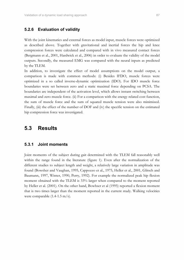
Validation of a dynamic load sharing approach 87
5.2.6 Evaluation of validity
With the joint kinematics and external forces as model input, muscle forces were optimized as described above. Together with gravitational and inertial forces the hip and knee compression forces were calculated and compared with in vivo measured contact forces (Bergmann et al., 2001, Hardwick et al., 2006) in order to evaluate the validity of the model outputs. Secondly, the measured EMG was compared with the neural inputs as predicted by the TLEM. In addition, to investigate the effect of model assumptions on the model output, a comparison is made with common methods: (i) Besides IFDO, muscle forces were optimized in a so called inverse-dynamic optimization (IDO). For IDO muscle force boundaries were set between zero and a static maximal force depending on PCSA. The boundaries are independent of the activation level, which allows instant switching between maximal and zero muscle force. (ii) For a comparison with the energy related cost function, the sum of muscle force and the sum of squared muscle tension were also minimized. Finally, (iii) the effect of the number of DOF and (iv) the specific tension on the estimated hip compression force was investigated.
5.3 Results
5.3.1 Joint moments
Joint moments of the subject during gait determined with the TLEM fall reasonably well within the range found in the literature (figure 1). Even after the normalization of the different studies to subject length and weight, a relatively large variation in amplitude was found (Bowsher and Vaughan, 1995, Cappozzo et al., 1975, Heller et al., 2001, Glitsch and Baumann, 1997, Winter, 1990, Perry, 1992). For example the normalized peak hip flexion moment obtained with the TLEM is 33% larger when compared to the moment reported by Heller et al. (2001). On the other hand, Bowhser et al (1995) reported a flexion moment that is two times larger than the moment reported in the current study. Walking velocities were comparable (1.4-1.5 m/s).
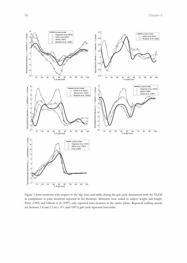
88 Chapter 5
% of gait cycle
Nor
mal
ized
hip
flex
ion
( ← )
/ ex
tens
ion
( → )
torq
ue
10 20 30 40 50 60 70 80 90 100−8
−6
−4
−2
0
2
4
6
8 current modelCappozzo et al.(1975)Heller et al.(2001)Winter (1991)Bowsher et al. (1995)
% of gait cycle
Nor
mal
ized
hip
inte
rnal
( ←
) /
exte
rnal
( →
) to
rque
10 20 30 40 50 60 70 80 90 100−0.6
−0.4
−0.2
0
0.2
0.4
0.6
0.8current modelHeller et al.(2001)Bowsher et al. (1995)
% of gait cycle
Nor
mal
ized
hip
add
uctio
n (
← )
/ ab
duct
ion
( →
) to
rque
10 20 30 40 50 60 70 80 90 100−2
−1
0
1
2
3
4
5
6
7
8current modelHeller et al. (2001)Glitsch et al. (1997)Bowsher et al. (1995)
% of gait cycle
Nor
mal
ized
kne
e ex
tens
ion
( ← )
/ fle
xion
( →
) to
rque
10 20 30 40 50 60 70 80 90 100−6
−5
−4
−3
−2
−1
0
1
2
3
4 current modelCappozzo et al. (1975)Winter (1990)Glitsch et al. (1997)
% of gait cycle
Nor
mal
ized
ank
le d
orsi
flexi
on (
← )
/ pl
anta
rfle
xion
( →
) to
rque
10 20 30 40 50 60 70 80 90 100−4
−2
0
2
4
6
8
10
12
14current modelCappozzo et al. (1975)Winter et al. (1991)Perry (1992)
Figure 1 Joint moments with respect to the hip, knee and ankle during the gait cycle determined with the TLEM in comparison to joint moments reported in the literature. Moments were scaled to subject weight and length. Perry (1992) and Glitsch et al. (1997) only reported joint moment in the stance phase. Reported walking speeds are between 1.4 and 1.5 m/s. 0% (and 100%) gait cycle represent heel strike
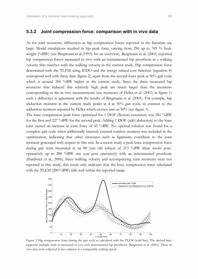
Validation of a dynamic load sharing approach 89
5.3.2 Joint compression force: comparison with in vivo data
As for joint moments, differences in hip compression forces reported in the literature are large. Model simulations resulted in hip peak force varying from 296 up to 769 % body weight (%BW) (see Bergmann et al (1993) for an overview). Bergmann et al. (2001) reported hip compression forces measured in vivo with an instrumented hip prosthesis at a walking velocity that matches with the walking velocity in the current study. Hip compression force determined with the TLEM using IFDO and the energy related cost function (equation 4) correspond well with these data (figure 2), apart from the second force peak at 50% gait cycle which is around 200 %BW higher in the current study. Since the three measured hip moments that induced this relatively high peak are much larger than the moments corresponding to the in vivo measurements (see moments of Heller et al. (2001) in figure 1) such a difference is agreement with the results of Bergmann et al. (2001). For example, hip abduction moment in the current study peaks at 4 at 50% gait cycle, in contrast to the adduction moment reported by Heller which crosses zero at 50% (see figure 1). The knee compression peak force optimized for 1 DOF (flexion/extension) was 281 %BW for the first and 227 %BW for the second peak. Adding 1 DOF (add/abduction) to the knee joint caused an increase in joint force of 45 %BW. No optimal solution was found for a complete gait cycle when additionally internal/external rotation moment was included in the optimization, indicating that other structures such as ligaments contribute to the joint moment generated with respect to this axis. In a recent study a peak knee compression force during gait were measured in an 80 year old subject of 213 %BW three weeks post-operatively up to 280 %BW one year post operatively with an instrumented prosthesis (Hardwick et al., 2006). Since walking velocity and accompanying joint moments were not reported in this study, this result only indicates that the knee compression force calculated with the TLEM (280 %BW) falls well within the reported range.
% of gait cycle
Hip
Com
pres
sion
For
ce (
% B
ody
Wei
ght)
10 20 30 40 50 60 70 80 90 1000
50
100
150
200
250
300
350
400
450
calculated with TLEMmeasured in vivo (Bergmann et al. (2001))
Figure 2 Hip compression force during the gait cycle as calculated with the TLEM (solid line). The dashed lines represent multiple trials as measured in vivo with instrumented hip prostheses (Bergmann et al. (2001). These in vivo data were collected in two subjects at a comparable walking speed.
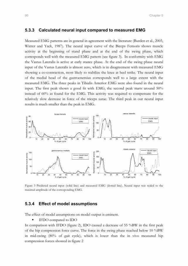
90 Chapter 5
5.3.3 Calculated neural input compared to measured EMG
Measured EMG patterns are in general in agreement with the literature (Burden et al., 2003, Winter and Yack, 1987). The neural input curve of the Biceps Femoris shows muscle activity at the beginning of stand phase and at the end of the swing phase, which corresponds well with the measured EMG pattern (see figure 3). In conformity with EMG the Vastus Lateralis is active at early stance phase. At the end of the swing phase neural input of the Vastus Lateralis is almost zero, which is in disagreement with measured EMG showing a co-contraction, most likely to stabilize the knee at heel strike. The neural input of the medial head of the gastrocnemius corresponds well to a large extent with the measured EMG. The three peaks in Tibialis Anterior EMG were also found in the neural input. The first peak shows a good fit with EMG, the second peak starts around 50% instead of 60% as found for the EMG. This activity was required to compensate for the relatively slow decrease in force of the triceps surae. The third peak in our neural input results is much smaller than the peak in EMG.
% of gait cycle
Nor
mal
ized
mus
cle
activ
ity
biceps femoris
10 20 30 40 50 60 70 80 90 1000
20
40
60
80neural inputEMG
% of gait cycle
Nor
mal
ized
mus
cle
activ
ity
vastus lateralis
10 20 30 40 50 60 70 80 90 1000
50
100
150neural inputEMG
% of gait cycle
Nor
mal
ized
mus
cle
activ
ity
gastrocnemius medialis
10 20 30 40 50 60 70 80 90 1000
50
100
150neural inputEMG
% of gait cycle
Nor
mal
ized
mus
cle
activ
ity
tibialis anterior
10 20 30 40 50 60 70 80 90 1000
50
100
150
200 neural inputEMG
Figure 3 Predicted neural input (solid line) and measured EMG (dotted line). Neural input was scaled to the maximal amplitude of the corresponding EMG.
5.3.4 Effect of model assumptions
The effect of model assumptions on model output is eminent. IFDO compared to IDO
In comparison with IFDO (figure 2), IDO caused a decrease of 55 %BW in the first peak of the hip compression force curve. The force in the swing phase reached below 10 %BW in mid-swing (80% of gait cycle), which is lower than the in vivo measured hip compression forces showed in figure 2

Validation of a dynamic load sharing approach 91
Cost function Differences in hip compression force for the three investigated cost functions were small (< 40 %BW). However, at the level of in individual muscle force, differences can be large (see figure 4). Smaller muscles are excluded or play a minor role when the muscle force is optimized with the mechanically related cost functions (minimization of sum of muscle forces or squared muscle stresses).
Number of DOFs included in the optimization In agreement with previous model simulations (Glitsch and Baumann, 1997) an increase in the number of DOFs in the optimization resulted in an increase in hip compression forces as more DOFs need to be equilibrated by the muscles. Including hip rotation moment in the optimization resulted in a maximal increase of 52 %BW in the first peak. Including the abduction moment in the optimization causes the largest increase in the second peak (152 %BW). Overall, the best fit with in vivo measured hip forces was obtained when the hip was modeled with 3 DOF.
Specific tension Compression force increased with specific muscle tension. For example when using a specific tension of 100 N/cm2 instead of 45 N/cm2 as in the current study, the first hip force peak increased with 99 %BW. A specific tension of 45 N/cm2 showed a better fit with in vivo measured compression forces and falls within the range of 15 – 47 N/m2 as reported in the literature (Fukunaga et al., 1996).
Figure 4 Muscle force during gait in the Biceps Femoris and Adductor Brevis, respectively a relatively large (245 gram) and small (115 gram) hip muscle. Since muscle mass is weighted, for the energy cost function the contribution of smaller muscles is larger and the contribution of larger muscles is smaller when compared to forces based on the two mechanically related cost functions (sum of muscle forces, sum of squared muscle stresses). Minimizing sum of muscle forces resulted in a force in the Biceps Femoris that is around 15 times larger than the force in the Adductor Brevis (respectively 475 and 30 N). With the energy cost function the force in the biceps is around 2 times the force in the Adductor Brevis (respectively 300 and 160 N).

92 Chapter 5
5.4 Discussion
In this study muscle forces are optimized using the TLEM, a recently introduced musculoskeletal model. The model can be distinguished from other models by its inverse forward dynamic optimization method, cost function and consistent anatomical data.
5.4.1 Accuracy and limitations of validation methods
Since direct measurement of muscle forces in vivo is difficult, typically musculoskeletal models are validated by comparing model output with EMG and joint compression forces. For quantitative validation of the predicted load sharing in vivo measured joint compression force is the only available source providing insight in the actual load acting on the joint. Unfortunately, the availability of these data is very limited. Just recently, the first in vivo collected knee compression forces were reported, measured using an instrumented tibial prosthesis (D'Lima et al., 2006, Hardwick et al., 2006). This makes a comparison of predicted knee compression forces possible. However, other accompanying biomechanical measures such as walking velocities and joint torques were not reported, which hampers an extensive inter-individual comparison. For the hip these data are available (Bergmann et al., 2001). Therefore, although collected on other subjects, these data provide more insight whether model outputs are reasonable or not. The comparison with EMG in this study is accurate. First, EMG and gait kinematics were measured simultaneously on the same subject which makes a comparison more straightforward than a comparison with EMG patterns from different subjects (e.g. (Thelen et al., 2003)). Secondly, EMG was compared with neural input instead of muscle as has been previously done (e.g. (Anderson and Pandy, 2001)). A comparison with neural input is more accurate as neural excitation and calcium dynamics are taken into account (figure 5).
% of gait cycle
Nor
mal
ized
mus
cle
activ
ity
Gastrocnemius Medialis
10 20 30 40 50 60 70 80 90 1000
20
40
60
80
100
120
140
EMGNeural inputForce
Figure 5 Measured EMG of the gastrocnemius medialis (thin solid line) compared to predicted neural input (thick line) and muscle force (dotted) both scaled to EMG amplitude, showing a better fit for the neural input due to the including of activation and excitation dynamics.

Validation of a dynamic load sharing approach 93
5.4.2 Anatomical model parameters
The prediction of muscle forces is highly dependent on the geometry of the model. In the ideal case anatomical parameters are subject-specific in order to account for architectural differences between subjects. However, with the available methods to obtain these data, such as MRI and CT, important muscle parameters such as optimal fiber length cannot be determined for an individual yet. Therefore musculoskeletal models are generally based on cadaver studies. The TLEM has three advantages when compared to other models. First, the model is based on an anatomical dataset comprising all relevant geometric parameters for muscle force estimation. Where other models (e.g. (Delp et al., 1990)) are constructed by merging different datasets and estimations of missing parameters such as optimal fiber length, the current model is based on consistent, experimentally obtained data (Klein Horsman et al., 2007a). Secondly, the TLEM consists of an extensive number of muscle elements which expand the possible solutions to share the load such that all DOF are involved; making the estimation of tissue load becomes more realistic. Muscle forces generating a required moment with respect to one axis might result in an unwanted moment with respect to another axis, requiring compensation by other muscles, causing an increase in joint force. An insufficient number of muscle elements results in an overestimation of the compression force. This effect explains the unrealistically high hip compression force (around 600 %BW) found by Glitsch and Baumann (1997) when optimizing 3 DOF in the hip using only 47 muscle elements (Brand et al., 1982). Finally, since force length characteristics are accurately implemented based on sarcomere length measurements, cost functions based on these parameters as presented by Praagman et al. (2006) can be implemented, which are likely to improve muscle force estimation. Scaling of the model to the subject is relevant in order to minimize anatomical differences between the model and the subject. Segment dimensions were scaled using externally measurable segment dimensions of the subject, which resulted in a more accurate joint moment determination. Internal anatomical properties such as muscle parameters and wrapping surfaces, important for estimation of muscle forces, were also scaled with these external measures. It is expected that scaling of these parameters minimizes anatomical differences and thus improves the accuracy of estimation of muscle forces. However, to what extent remains uncertain, as these parameters could not be measured.
5.4.3 IFDO
IFDO is a fast and stable algorithm for inverse-dynamic optimization. In comparison to IDO, as for example used by Heller et al. (2001) for estimation of hip compression forces, IFDO only allows changes in muscle force that agree with excitation and activation dynamics (figure 6). For example in the gluteus medius, the difference in boundaries of

94 Chapter 5
muscle force for IFDO and IDO resulted for IDO in unrealistic muscle force patterns and changes. IFDO resulted in neural inputs that agreed well with EMG measurements. Although Heller et al. (2001) found a good fit of predicted hip forces with experimental data, the utilization of IDO and a cost function minimizing sum of muscle forces, the unreported individual muscle forces are most likely not in agreement with EMG. Anderson and Pandy (2001) used a forward dynamic musculoskeletal model to optimize muscle activations by minimizing metabolic energy. Simulated moments were used as an input in a static model and it was concluded that static and dynamic optimization is practically equivalent. This statement is in disagreement with the findings in this study. One explanation is that only one cost function was investigated in the study of Anderson. Cost functions like the minimization of the sum of muscle force as used by Heller et al. (2001) resulted in large differences in muscle force between static and dynamic optimization in the current study. Furthermore the study of Anderson is based on simulated moments instead of joint torques based on experimental data as in the current study. This underrates the relevance of muscle dynamics.
% of gait cycle
Opt
imiz
ed G
lute
us M
ediu
s Fo
rce
and
boun
derie
s (N
)
10 20 30 40 50 60 70 80 90 100-50
0
50
100
150
200
250
Muscle force IFDOMuscle force IDOEMG
Figure 6 Muscle force optimized according IFDO (black solid) and IDO (black dotted) falling between the corresponding optimization boundaries (subsequently dark and light grey area). Boundaries for IFDO depend on the states of the muscle (equation 1 and 2). For IDO muscle forces is bounded between zero and maximal force (specific muscle tension * PCSA). Muscle forces determined with IDO show unrealistic fast transitions in muscle force. The solution space for IFDO is much smaller resulting in a different, more realistic muscle force. The solid light grey line shows the EMG (Winter and Yack, 1987).
Validation of a dynamic load sharing approach 95
5.4.4 Cost function
Praagman et al. (2006) experimentally showed that for shoulder muscles the energy related cost function (equation 4) has a better correspondence with energy consumption than stress related functions. Besides this energy function, two other frequently used functions were implemented in the current study. Minimizing the sum of muscle forces (e.g. (Crowninshield, 1978, Heller et al., 2001)) results in physiologically unrealistic muscle recruitment showing only activity in the muscle with largest moment arm. The minimization of squared muscle stresses caused more synergistic activity and a much better fit with EMG. A drawback of this criterion is that the load was not attributed to smaller muscles, as small PCSA cause larger unwanted stresses. The energy related cost function includes muscle mass and fiber length as a measure for the total number of binding cross-bridges. This makes the use of smaller muscle preferable, besides muscles with large moment arms and PCSA. It is expected that this corresponds more closely to actual load sharing. However, this could not be proven in the current study as the surface EMG of small muscles could not be measured sufficiently accurate.
5.4.5 Concluding remarks
In this study dynamic muscle parameters were incorporated in the TLEM, a comprehensive musculoskeletal model of the lower extremity based on extensive and accurate anatomical model parameters. Muscle forces during gait were optimized in a novel approach using IFDO in combination with an energy related cost function, which resulted in a stable and fast estimation of muscle forces during gait. Measured EMG agreed reasonably well with predicted neural inputs. Estimated joint compression forces are in agreement with in vivo data and can therefore be considered as trustworthy.
5.5 References
An, K. N., Kwak, B. M., Chao, E. Y.,Morrey, B. F., 1984. Determination of muscle and joint forces: a new technique to solve the indeterminate problem. Journal of Biomechanical Engineering, 106, 364-7.
Anderson, F. C.,Pandy, M. G., 1999. A Dynamic Optimization Solution for Vertical Jumping in Three Dimensions. Computer Methods Biomechanics and Biomedical Engineering, 2, 201-231.
Anderson, F. C.,Pandy, M. G., 2001. Static and dynamic optimization solutions for gait are practically equivalent. Journal of Biomechanics, 34, 153-61.
Bergmann, G., Deuretzbacher, G., Heller, M., Graichen, F., Rohlmann, A., Strauss, J.,Duda, G. N., 2001. Hip contact forces and gait patterns from routine activities. Journal of Biomechanics, 34, 859-71.
96 Chapter 5
Bowsher, K. A.,Vaughan, C. L., 1995. Effect of foot-progression angle on hip joint moments during gait. Journal of Biomechanics, 28, 759-62.
Brand, R. A., R.D., C., Wittstock, C. E., Pedersen, D. R., Clark, C. R.,Van Krieken, F. M., 1982. A model of the lower extremity muscular anatomy. Journal of Biomechanical Engineering, 104, 304-310.
Burden, A. M., Trew, M.,Baltzopoulos, V., 2003. Normalisation of gait EMGs: a re-examination. Journal of Electromyography and Kinesiology, 13, 519-32.
Cappozzo, A., Leo, T.,Pedotti, A., 1975. A general computing method for the analysis of human locomotion. Journal of Biomechanics, 8, 307-20.
Chandler, R. F., Clauser, C. E., Mcconville, J. T., Reynolds, H. M.,Young, J. W., 1975. Investigation of inertial properties of the human body. Report DOT HS-801430, National Technical Information Service, Springfield Virginia 22151, USA.
Crowninshield, R. D., 1978. Use of optimization techniques to predict muscle forces. Journal of Biomechanical Engineering, 100, 88-92.
Crowninshield, R. D.,Brand, R. A., 1981. A physiologically based criterion of muscle force prediction in locomotion. Journal of Biomechanics, 14, 793-801.
D'lima, D. D., Patil, S., Steklov, N., Slamin, J. E.,Colwell, C. W., Jr., 2006. Tibial forces measured in vivo after total knee arthroplasty. Journal of Arthroplasty, 21, 255-62.
Delp, S. L., Loan, J. P., Hoy, M. G., Zajac, F. E., Topp, E. L.,Rosen, J. M., 1990. An interactive graphics-based model of the lower extremity to study orthopaedic surgical procedures. IEEE Transactions on Biomedical Engineering, 37, 757-67.
Erdemir, A., Mclean, S., Herzog, W.,Van Den Bogert, A. J., 2007. Model-based estimation of muscle forces exerted during movements. Clinical Biomechanics (Bristol, Avon), 22, 131-54.
Fukunaga, T., Roy, R. R., Shellock, F. G., Hodgson, J. A.,Edgerton, V. R., 1996. Specific tension of human plantar flexors and dorsiflexors. Journal of Applied Physiology, 80, 158-65.
Glitsch, U.,Baumann, W., 1997. The three-dimensional determination of internal loads in the lower extremity. Journal of Biomechanics, 30, 1123-31.
Hardwick, M. E., Pulido, P. A., D'lima, D. D.,Colwell, C. W., Jr., 2006. e-Knee: the electronic knee prosthesis. Orthopaedic Nursing, 25, 326-9.
Heller, M. O., Bergmann, G., Deuretzbacher, G., Durselen, L., Pohl, M., Claes, L., Haas, N. P.,Duda, G. N., 2001. Musculo-skeletal loading conditions at the hip during walking and stair climbing. Journal of Biomechanics, 34, 883-93.
Hermens, H. J., Freriks, B., Disselhorst-Klug, C.,Rau, G., 2000. Development of recommendations for SEMG sensors and sensor placement procedures. Journal of Electromyography and Kinesiology, 10, 361-74.
Klein Horsman, M. D., Koopman, H. F., Van Der Helm, F. C., Prose, L. P.,Veeger, H. E., 2007a. Morphological muscle and joint parameters for musculoskeletal modelling of the lower extremity. Clinical Biomechanics (Bristol, Avon), 22, 239-47.
Klein Horsman, M. D., Koopman, H. F. J. M., Veeger, H. E. J.,Van Der Helm, F. C. T., 2007b. Musculoskeletal model of the lower extremity: a comparison of muscle moment arms with the literature. IEEE Transactions on Biomedical Engineering [submitted].
Klein Horsman, M. D., Koopman, H. F. J. M., Veeger, H. E. J.,Van Der Helm, F. C. T., 2007c. Musculoskeletal model of the lower extremity: comparison of maximal isometric moment with the literature. Journal of Biomechanics [submitted].
Koopman, B. (1989) The three-dimensional analysis and prediction of human walking. PhD Thesis, University of Twente, Enschede.

Validation of a dynamic load sharing approach 97
Koopman, B., Grootenboer, H. J.,De Jongh, H. J., 1995. An inverse dynamics model for the analysis, reconstruction and prediction of bipedal walking. Journal of Biomechanics, 28, 1369-76.
Li, G., Kaufman, K. R., Chao, E. Y.,Rubash, H. E., 1999. Prediction of antagonistic muscle forces using inverse dynamic optimization during flexion/extension of the knee. Journal of Biomechanical Engineering, 121, 316-22.
Pedersen, D. R., Brand, R. A.,Davy, D. T., 1997. Pelvic muscle and acetabular contact forces during gait. Journal of Biomechanics, 30, 959-65.
Perry, J. 1992 Gait Analysis: Normal and Pathological Function, New York, McGraw Hill, Inc.
Praagman, M., Chadwick, E. K., Van Der Helm, F. C.,Veeger, H. E., 2006. The relationship between two different mechanical cost functions and muscle oxygen consumption. Journal of Biomechanics, 39, 758-65.
Thelen, D. G., Anderson, F. C.,Delp, S. L., 2003. Generating dynamic simulations of movement using computed muscle control. Journal of Biomechanics, 36, 321-8.
Tsirakos, D., Baltzopoulos, V.,Bartlett, R., 1997. Inverse optimization: functional and physiological considerations related to the force-sharing problem. Critical Reviews in Biomedical Engineering, 25, 371-407.
Van Der Kooij, H.,Van Der Helm, F. C. (2003) Human gait analysis application of a new inverse/forward dynamic optimization (IFDO) method to solve the load sharing problem. International symposium on computer simulation in biomechanics. Sydney.
Winter, D. A. 1990 Biomechanics and motor control of human movement, Toronto, John Wiley & Sons, Inc.
Winter, D. A.,Yack, H. J., 1987. EMG profiles during normal human walking: stride-to-stride and inter-subject variability. Electroencephalography and Clinical Neurophysiology, 67, 402-11.
Winters, J. M.,Stark, L., 1985. Analysis of fundamental human movement patterns through the use of in-depth antagonistic muscle models. IEEE Transactions on Biomedical Engineering, 32, 826-39.
Winters, J. M.,Stark, L., 1988. Estimated mechanical properties of synergistic muscles involved in movements of a variety of human joints. Journal of Biomechanics, 21, 1027-41.
Yamaguchi, G. T., Sawa, A. G. U., Moran, D. W., Fessler, M. J.,Winters, J. M., 1990. A survey of human musculotendon actuator parameters, in: Winter, J. M. & Woo, S. L. Y. (Eds.) Multiple Muscle Systems: Biomechanics and Movement Organisation. Springer, Berlin, pp. 717-773.


Chapter 6
Relation between proximal femur deformities and
paralysis of hip abductors in children with
myelomeningocele
Abstract
Children with myelomeningocele frequently develop (sub-)luxated hip joints due to an increased angle between the neck and the shaft of the femur. More insight in the cause of this deformation would improve treatment methods such as tendon transfers. It was hypothesized that this femur deformation is caused by a more vertically oriented hip compression force in myelomeningocele patients as a result of paralysis of hip abductors. The goal of this study is to investigate if the force patterns on the hip after paralysis are in agreement with this hypothesis. Stance and gait were measured with a video system in 4 healthy children and 4 children with lower lumbo-sacral myelomeningocele. The measured joint angles were used as input in a comprehensive musculoskeletal model of the lower extremity in order to determine muscle forces, hip compression force and moments on the physis. Externally measurable segment dimensions, medical history and the measured EMG signals were used to scale the model to each individual subject. Results for healthy children were consistent and in agreement with the literature. Myelomeningocele patients showed a reduced hip abduction moment and in some cases even adduction moments during gait. It was shown that by including the patient’s pathological deficiencies in the model, healthy joint torques could not be generated by the muscles in the model. This is an indication that the patient is forced to walk the deviated Trendelenburg gait due to a lack of abduction force. Abnormal joint torques resulted in abnormal amplitudes of the compressive force during gait (up to 524 %BW). In general no significant differences in direction of the hip compression force were found between the healthy subject and the patients so the hypothesized cause of the femur neck deformities could not be confirmed. With more extensive scaling routines based on 3D images of bone geometries, femur deformations of a patient can be included in the model. It is expected that this will result in a better scaling of the muscle lines of action such that muscle force and hip compression can be estimated more accurately. This will possibly give more insight in the validity of the hypothesis.

Hip compression forces in Myelomeningocele patients 101
6.1 Introduction
The most common condition of spina bifida aperta is myelomeningocele in which meninges and nerves pass through an opening in the spinal canal. Proportional with the level of the lesion, this deficiency causes severe damage to nerves of the lower extremity, resulting in a paralysis of the corresponding muscles. Children with a lesion above L3 have a minimal potential to walk, due to a paralysis of the lower limb muscles. In general with a lesion below L5 children are able to walk normally (Rueda and Carroll, 1972). Patients with a lesion level L3-L4 have a so-called Trendelenburg gait in which the trunk is laterally rotated to counterbalance a paralysis of abductors. Hip adductors and flexors can still generate active force, allowing the children to walk. In almost all cases these patients develop an increased valgus angle of the femur neck causing luxations of the hip joint and consequential walking disabilities (Sharrard, 1964) (figure 1). Tendon transfers have been used to restore or prevent hip luxations. These procedures aim to improve walking capability by substituting the action of the paralyzed muscles and removing the cause of the deformation. Different methods are described in the literature, for example a lateral iliopsoas tendon transfer to below the trochanter major (Mustard, 1952). Sharrard found that this approach failed to prevent recurrent luxation of the hip joint in children with complete paralysis of the glutei muscles. He proposed a posterior m. iliopsoas transfer (Sharrard, 1964). Several studies showed a reduction of the deformities and an improvement of ambulatory status after this procedure (Sharrard, 1964, Carroll and Sharrard, 1972, Menelaus, 1969, Stillwell and Menelaus, 1984, Lorente Molto and Martinez Garrido, 2005, Breed and Healy, 1982, Lee and Carroll, 1985). Others recommended procedures involving a combination of muscle lengthening or transfer of the tensor fascia latae, the external oblique, vastus lateralis, rectus femoris and sartorius (Cabaud et al., 1979, Beaty and Canale, 1990). Despite the multiple operational methods, re-luxation of the hip after operation still occurs in 4% (Lee and Carroll, 1985) to 40% (Feiwell et al., 1978) of the myelomeningocele patients. More insight in the relation between abnormal muscle forces and the femoral deformities in children with myelomeningocele is therefore needed. A plausible cause of the hip (sub)-luxations is a disturbance in the longitudinal growth of the femoral neck due to diminished abductor force, resulting in a more vertical orientation of the femoral neck, as hypothesized in figure 1. Since the center of mass is placed above the hip joint in myelomeningocele patients, the hip compression force becomes more vertical. This causes an increased torque on the physis resulting in more compression force on the medial side of the femur neck. According the growth curve in figure 2 (Frost, 1997) an increased compression force causes more longitudinal growth on the medial side, resulting in a coxa valga: an increased valgus angle of the femur neck. If this hypothesis can be proven tendon transfer procedures can be optimized and more successful results can be obtained.

102 Chapter 6
A B
D C
FmusFmus
Fmus
Fmus
FhipFhip
Fhip
Fhip
Fgrf Fgrf
FgrfFgrf
COM COM
COMCOM
Figure 1 At the top, an anterior-posterior radiograph of a healthy subject (left) and a myelomeningocele patient showing a coxa valga that causes hip (sub-)luxations. Below, 4 schematic drawings of the forces acting on the femur during single stance phase in the gait cycle, showing the hypothesized cause of deformations in the neck of the femur. A) Healthy subject: The ground reaction force runs through the center of mass and exerts a torque on the hip. To maintain moment equilibrium muscles generate a counterbalancing force. The hip compression force maintains the force equilibrium on the femur. The black dot represents the physis with the corresponding distributed load. B) Damaged nerves diminish the force in the hip in myelomeningocele patients. Gait pattern is adapted such that the COM is closer to the hip and the resulting torque can be counterbalanced. The resulting hip compression force causes a deviated load distribution on the physis. C) According to the growth force response reported by Frost et al. (1997) increased compression force initiates longitudinal growth, which re-aligns the femur neck with the load and results in (sub-)luxation of the hip. D) Tendon transfer is aimed to restore the action of the paralyzed muscles and reduce deformities in order to walking capabilities of the patient.
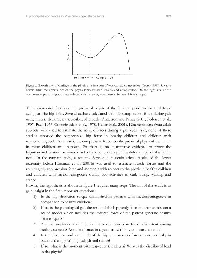
Hip compression forces in Myelomeningocele patients 103
Figure 2 Growth rate of cartilage in the physis as a function of tension and compression (Frost (1997)). Up to a certain limit, the growth rate of the physis increases with tension and compression. On the right side of the compression peak the growth rate reduces with increasing compression force and finally stops. The compressive forces on the proximal physis of the femur depend on the total force acting on the hip joint. Several authors calculated this hip compression force during gait using inverse dynamic musculoskeletal models (Anderson and Pandy, 2001, Pedersen et al., 1997, Paul, 1976, Crowninshield et al., 1978, Heller et al., 2001). Kinematic data from adult subjects were used to estimate the muscle forces during a gait cycle. Yet, none of these studies reported the compressive hip force in healthy children and children with myelomeningocele. As a result, the compressive forces on the proximal physis of the femur in these children are unknown. So there is no quantitative evidence to prove the hypothesized relation between a lack of abduction force and a deformation of the femur neck. In the current study, a recently developed musculoskeletal model of the lower extremity (Klein Horsman et al., 2007b) was used to estimate muscle forces and the resulting hip compression force and moments with respect to the physis in healthy children and children with myelomeningocele during two activities in daily living; walking and stance. Proving the hypothesis as shown in figure 1 requires many steps. The aim of this study is to gain insight in the first important questions:
1) Is the hip abduction torque diminished in patients with myelomeningocele in comparison to healthy children?
2) If so, is the pathological gait the result of the hip paralysis or in other words can a scaled model which includes the reduced force of the patient generate healthy joint torques?
3) Are the amplitude and direction of hip compression forces consistent among healthy subjects? Are these forces in agreement with in vivo measurements?
4) Is the direction and amplitude of the hip compression forces more vertically in patients during pathological gait and stance?
5) If so, what is the moment with respect to the physis? What is the distributed load in the physis?
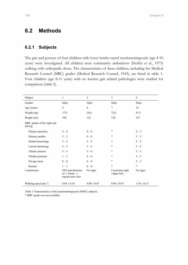
104 Chapter 6
6.2 Methods
6.2.1 Subjects
The gait and posture of four children with lower lumbo-sacral myelomeningocele (age 4-10 years) were investigated. All children were community ambulators (Hoffer et al., 1973) walking with orthopedic shoes. The characteristics of these children, including the Medical Research Council (MRC) grades (Medical Research Council, 1943), are listed in table 1. Four children (age 8-11 years) with no known gait related pathologies were studied for comparison (table 2).
Subject 1 2 3 4
Gender Male Male Male Male
Age (years) 4 6 7 10
Weight (kg) 17.0 26.0 22.0 41.5
Height (cm) 104 122 120 147
MRC grades of the right and left leg
Gluteus maximus 4 – 4 0 – 0 * 2 – 3
Gluteus medius 2 – 2 0 – 0 * 3 – 3
Medial hamstrings 5 – 5 5 – 5 * 5 – 5
Lateral hamstrings 5 – 5 5 – 5 * 5 – 5
Tibialis anterior 5 – 5 5 – 0 * 5 – 5
Tibialis posterior 1 – 1 4 – 0 * 5 – 5
Triceps surae 0 – 0 0 – 0 * 2 – 3
Peronei 1 – 1 0 – 0 * * Contractures 50% lateralization
of r. femur, r. equinovarus foot
No signs Correction right valgus foot
No signs
Walking speed (ms-1) 0.84 ± 0.10 0.80 ± 0.07 0.84 ± 0.07 1.34 ± 0.15 Table 1 Characteristics of the myelomeningocele (MMC) subjects. * MRC grade was not available.

Hip compression forces in Myelomeningocele patients 105
The local ethics committee of Roessingh Rehabilitation Clinic approved this research project and informed consent from the parents was obtained before each measurement.
6.2.2 Measurement of kinematics
All subjects performed 2 trials standing with their right leg on a force platform. Subsequently each subject walked at least ten times over a walkway. The corresponding 3D kinematics were recorded using six infrared cameras (VICON, Oxford Metrics, Oxford, U.K., 100 Hz) and two AMTI force platforms (Watertown, MA, 1000 Hz). Surface EMG of the following right leg muscles were measured: m. gluteus maximus, m. gluteus medius, m. rectus femoris, m. vastus lateralis, m. biceps femoris, m. semitendinosus, m. gastrocnemius and m. tibialis anterior. A reference electrode was placed around the wrist. The surface electrodes were placed in accordance with the Seniam recommendations (Hermens et al., 2000). A 16-channel EMG system (K-lab, Kinesiologic laboratory system, Amsterdam, 1000 Hz) recorded the EMG signals. The raw EMG signals were filtered with a high pass filter (3rd order, zero-phase lag, cut-off, Butterworth, 20 Hz), then rectified, low pass filtered (2nd order, zero-phase lag, cut-off, Butterworth, 25 Hz) and interpolated. The joint angles were determined using an inverse rigid-body dynamic model (Koopman et al., 1995). Kinematic data and ground reaction forces were low pass filtered (2nd order, zero-phase lag, cut-off, Butterworth, 5 Hz).
6.2.3 Twente Lower Extremity Model
The Twente Lower Extremity Model (TLEM), a recently developed musculoskeletal model of the lower extremity was used to estimate hip compression force of the measured movements. This model is based on an extensive anatomical dataset of a right lower extremity (Klein Horsman et al., 2007a). The model consists of 12 body segments: HAT (head, arms and trunk), pelvis and the left and right femur, patella, tibia, talus and foot. There are 21 degrees of freedom (DOF) described in the model: the L5S1 joint and the left
1 2 3 4
Gender Male Male Male Male
Age (years) 8 8 10 11
Weight (kg) 36.0 34.0 34.5 48.0
Height (cm) 147 139 150 164
Walking speed (ms-1) 1.02 ± 0.04 1.15 ± 0.09 1.38 ± 0.03 1.43 ± 0.07 Table 2 Characteristics of the healthy (H) subjects.

106 Chapter 6
and right hip with 3 DOF and the left and right knee, talocrural and subtalar joint with 1 DOF. To describe the mechanical effect of the 76 lower limb muscles in both lower extremities, 264 Hill type muscle elements are defined. A muscle element is determined by the position of the origin and insertion. Muscle parameters such as muscle mass, pennation angle, physical cross-sectional area (PCSA), tendon length and optimal fiber length, are assigned to each muscle. A more detailed description of the TLEM is given in a previous study (Klein Horsman et al., 2007b). The model has been validated by comparing muscle moment arms, maximal isometric moments, joint forces and neural inputs with data in literature (Klein Horsman et al., 2007b, Klein Horsman et al., 2007c, Klein Horsman et al., 2007d).
6.2.4 Scaling
The TLEM was scaled to each individual subject. The segments were scaled such that the bony landmarks as defined in the musculoskeletal model fit with the bony landmarks as measured on the subject in an upright pose. As a consequence of segment scaling the muscle lengths changed. The ratios between the scaled and original muscle lengths were used to scale the tendon lengths and the muscle optimal fiber lengths. The muscle mass was scaled linearly with the mass ratio and the PCSA with the mass and height ratio. In the myelomeningocele subjects the innervations of some muscles was limited. The lesion level and MRC grades reported in the medical history and the measured EMG signals were used to determine the innervation level of these muscles. The innervation levels were used to linearly diminish the maximal force these muscles could generate in the musculoskeletal model.
6.2.5 Model simulations
This study consisted of 5 different model simulations: Simulation of healthy gait kinematics with the TLEM scaled to the corresponding
healthy subjects; Simulation of pathological gait kinematics with the TLEM scaled to the
corresponding myelomeningocele patients; Simulation of healthy gait kinematics with the TLEM scaled to myelomeningocele
patients; Simulation of healthy stance in with the TLEM scaled to corresponding healthy
subjects; Simulation of pathological stance with the TLEM scaled to corresponding
myelomeningocele patients.
Hip compression forces in Myelomeningocele patients 107
6.2.6 Hip compressive force and physeal moment
An inverse-forward dynamic optimization (IFDO) method was used to estimate muscle forces (Van Der Kooij, 2003, Klein Horsman et al., 2007d). This inverse optimization method uses a forward muscle model to account for muscle dynamics. The distribution of the muscle forces was determined by an optimization of an energy related cost function (Praagman et al., 2006). Hip compression force was calculated by summing all forces on the femur: the optimized muscle forces, the external forces and inertial and gravitational forces. The physeal moments were defined as the cross product of the hip compression force vector and a moment arm vector from the hip to a fixed point on the physis. The location of the physis is not included in the anatomical dataset of Klein Horsman et al. (2007a) and therefore assumed in the middle of the trochanter major and the rotation center of the hip joint.
6.3 Results
A representative gait and stance trial of each subject was chosen for data presentation.
6.3.1 Joint angles
The joint angles of the healthy (H) subjects are in line with the ranges found in literature (e.g.(van der Linden ML et al., 2002, Gutierrez et al., 2003, Winter, 1991)). The joint angles of the myelomeningocele (MMC) subjects varied (figure 3). These variations are probably caused by small differences in muscle paresis around the ankle and hip joint (Gutierrez et al., 2005). The joint angles of MMC subject 3 and 4 showed relatively small deviations from normal. Mainly sagittal plane differences were observed. The gait pattern of MMC subject 1 and 2 were markedly different. They showed a hip abduction position during stance, whereas it was adduction in healthy subjects. The knee joint of MMC subject 1 was also more flexed during stance and the ankle was persistent slightly dorsal flexed (figure 3).
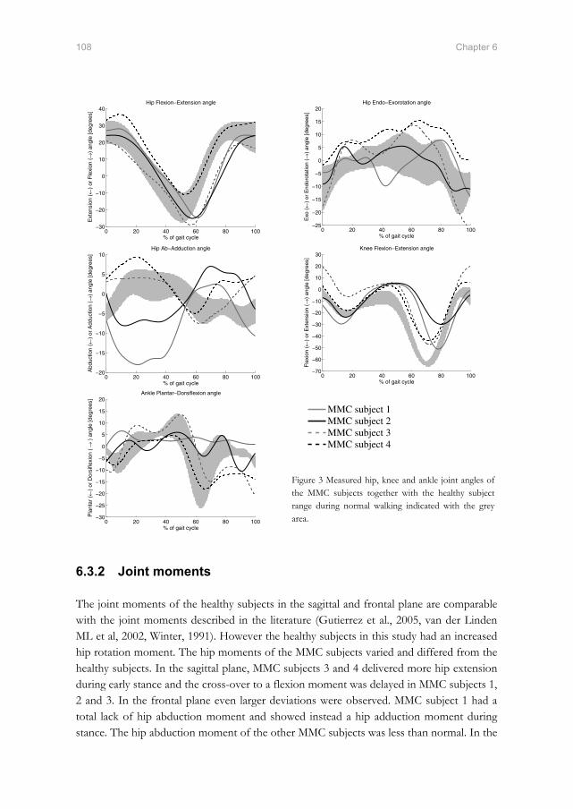
108 Chapter 6
0 20 40 60 80 100−30
−20
−10
0
10
20
30
40Hip Flexion−Extension angle
% of gait cycle
Ext
ensi
on (
←)
or F
lexi
on (→
) an
gle
[deg
rees
]
0 20 40 60 80 100
−25
−20
−15
−10
−5
0
5
10
15
20Hip Endo−Exorotation angle
% of gait cycle
Exo
(←
) or
End
orot
atio
n (→
) an
gle
[deg
rees
]
0 20 40 60 80 100−20
−15
−10
−5
0
5
10Hip Ab−Adduction angle
% of gait cycle
Abd
uctio
n (←
) or
Add
uctio
n (→
) an
gle
[deg
rees
]
0 20 40 60 80 100
−70
−60
−50
−40
−30
−20
−10
0
10
20
30Knee Flexion−Extension angle
% of gait cycle
Fle
xion
(←)
or E
xten
sion
(→
) an
gle
[deg
rees
]
0 20 40 60 80 100−30
−25
−20
−15
−10
−5
0
5
10
15
20Ankle Plantar−Dorsiflexion angle
% of gait cycle
Pla
ntar
(←
) or
Dor
sifle
xion
( →
) a
ngle
[deg
rees
]
MMC subject 1MMC subject 2MMC subject 3MMC subject 4
Figure 3 Measured hip, knee and ankle joint angles of the MMC subjects together with the healthy subject range during normal walking indicated with the grey area.
6.3.2 Joint moments
The joint moments of the healthy subjects in the sagittal and frontal plane are comparable with the joint moments described in the literature (Gutierrez et al., 2005, van der Linden ML et al, 2002, Winter, 1991). However the healthy subjects in this study had an increased hip rotation moment. The hip moments of the MMC subjects varied and differed from the healthy subjects. In the sagittal plane, MMC subjects 3 and 4 delivered more hip extension during early stance and the cross-over to a flexion moment was delayed in MMC subjects 1, 2 and 3. In the frontal plane even larger deviations were observed. MMC subject 1 had a total lack of hip abduction moment and showed instead a hip adduction moment during stance. The hip abduction moment of the other MMC subjects was less than normal. In the

Hip compression forces in Myelomeningocele patients 109
transversal plane, the profile of the hip rotation moment was altered in MMC subjects 1 and 2. A hip external rotation moment was observed during the first 25% of the gait cycle, whereas healthy subjects showed an internal rotation moment (figure 4). The knee moments of the MMC subjects also varied from normal. During early stance the knee extension moment of MMC subjects 2 and 4 was larger than that of the healthy subjects. The average knee extension moment of MMC subject 4 was even more than twice as large. During late stance MMC subjects 2, 3 and 4 showed less knee flexion moment. MMC subject 4 maintained knee extension throughout the whole stance phase, so no flexion moment was generated during late stance (figure 4). The ankle moment of the MMC subjects showed a smaller peak plantar flexion moment than in the healthy subjects.
0 20 40 60 80 100−6
−4
−2
0
2
4
6
8Hip Flexion−Extension moment
% of gait cycle
Fle
xion
(←)
or E
xten
sion
(→
) m
omen
t
0 20 40 60 80 100−2
−1
0
1
2
3
4
5Hip Endo−Exorotation moment
% of gait cycle
Inte
rnal
(←
) or
Ext
erna
l (→
) m
omen
t
0 20 40 60 80 100−3
−2
−1
0
1
2
3
4
5Hip Ab−Adduction moment
% of gait cycle
Add
uctio
n (←
) or
Abd
uctio
n (→
) m
omen
t
0 20 40 60 80 100−12
−10
−8
−6
−4
−2
0
2
4Knee Flexion−Extension moment
% of gait cycle
Ext
ensi
on (
←)
or F
lexi
on (→
) m
omen
t
0 20 40 60 80 100−2
0
2
4
6
8
10
12
14Ankle Plantar−Dorsiflexion moment
% of gait cycle
Dor
si (
←)
or P
lant
arfle
xion
(→)
mom
ent
Figure 4 Calculated hip, knee and ankle joint moments of the MMC subjects together with the healthy subject range during normal walking indicated with the grey area. The joint moments were normalized to subject length and weight.
MMC subject 1MMC subject 2MMC subject 3MMC subject 4

110 Chapter 6
6.3.3 Amplitude of the hip compressive force
The healthy children showed a hip compressive force amplitude (scaled to body weight) that is in agreement with in vivo measured hip compressive forces of elderly patients with a hip implant (Bergmann et al., 2001) (figure 5). Healthy subject 3 showed increased hip joint moments during stance. Therefore the hip compressive force of this subject was larger compared to the other subjects. As for the joint moments, the variations between the hip compressive force of the MMC and healthy subjects are considerable (figure 5). The hip compressive force of these subjects showed less clearly the characteristically two-peak form with peak values up to 524 %BW. MMC subject 1 showed large deviating hip moments, especially during mid and late stance. This made determination of the hip compressive force impossible since the muscle force could not be generated by the TLEM. During early stance the hip compressive force could be determined. The first peak in the hip compressive force, just after heel strike, had an amplitude of 338 %BW.
6.3.4 Direction of the hip compressive force
In the healthy subjects the average direction of the hip compressive force was consistent (table 3). The inclinations angles were slightly smaller compared to in vivo measurements (Bergmann et al., 2001). MMC subject 3 showed similar inclination angles as the healthy subjects, but the inclination angles of MMC subjects 2 and 4 differed (table 3). As an example, the range and the mean inclination angles of the average healthy subject and MMC subject 4 are displayed in figure 6.
Figure 5 On the left calculated hip compressive force of the healthy subjects and in vivo measured hip compressive forces (Bergmann et al., 2001) during normal walking. The in vivo data were obtained with an average walking speed of 1.09 ms-1. All forces were normalized to subject weight. On the right calculated hip compressive force of the MMC subjects during normal walking. The forces were normalized to subject weight.

Hip compression forces in Myelomeningocele patients 111
Figure 6 The directions of the hip compressive force for the average healthy subject and MMC subject 4. Subject Angle in the frontal plane
(Degrees) Angle in the sagittal plane (Degrees)
Angle in the transverse plane (Degrees)
Healthy subject 1 16.6 ± 8.7 6.2 ± 11.3 14.2 ± 28.5
Healthy subject 2 16.6 ± 10.2 6.8 ± 10.3 17.1 ± 27.5
Healthy subject 3 19.1 ± 8.4 7.8 ± 7.7 17.5 ± 20.1
Healthy subject 4 16.9 ± 8.2 7.7 ± 7.3 22.2 ± 21.5
MMC subject 1* - - -
MMC subject 2 14.9 ± 10.5 10.6 ± 10.1 37.6 ± 32.7
MMC subject 3 16.9 ± 9.6 6.1 ± 7.2 17.2 ± 21.9
MMC subject 4 21.0 ± 8.9 11.6 ± 7.8 27.3 ± 14.4
Table 3 Mean and standard deviation of the normalized hip compressive force inclination angles during normal walking. * The dynamic optimization problem could not be solved for the whole gait cycle.
6.3.5 Physeal moments
The healthy subjects, except subject 3, showed consistent physeal moments. As for the joint moments and the hip compressive force, the physeal moments of healthy subject 3 were slightly larger. The physeal moments of the MMC subjects were on average slightly larger compared to the healthy subjects (table 4).

112 Chapter 6
Subject Moment around local x-axis
Moment around local y-axis
Moment around local z-axis
Healthy subject 1 2.11 ± 0.76 0.05 ± 0.11 0.12 ± 0.29
Healthy subject 2 2.14 ± 0.71 0.05 ± 0.10 0.14 ± 0.28
Healthy subject 3 3.20 ± 1.34 0.14 ± 0.14 0.36 ± 0.39
Healthy subject 4 2.50 ± 0.88 0.09 ± 0.08 0.27 ± 0.27
MMC subject 1* - - -
MMC subject 2 2.46 ± 1.23 0.13 ± 0.11 0.41 ± 0.33
MMC subject 3 3.37 ± 1.36 0.08 ± 0.09 0.25 ± 0.28
MMC subject 4 2.24 ± 1.02 0.12 ± 0.09 0.32 ± 0.24
Table 4 Mean and standard deviation of the physeal moments around a fixed point during normal walking. The moments are presented in the coordinate frame of the femur (Wu et al., 2002) and were normalized to subject length and weight. * The dynamic optimization problem could not be solved for the whole gait cycle.
6.3.6 Stance: Hip compressive force and physeal moment
During stance the amplitude of the hip compressive force was for the healthy as well as the MMC subjects nearly constant (figure 7). The amplitude of the healthy subjects showed only small variations. Their average amplitude was 93.5 %BW. The MMC subjects showed large variation in hip compressive force amplitude. The amplitude of MMC subject 3 was rather small because this subject placed most of his weight on his left foot. The hip compressive force of MMC subject 1 could not be determined. As for the gait trial, the TLEM was not able to solve the dynamic optimization problem.

Hip compression forces in Myelomeningocele patients 113
Figure 7 Left, calculated hip compressive force of the healthy subjects during stance. The forces were normalized to subject weight. Right, calculated hip compressive force of the MMC subjects during stance. The forces were normalized to subject weight. The direction of the hip compressive force was nearly constant during stance. However the average direction largely varied between the subjects, especially in the sagittal and frontal plane (table 5). In the frontal plane, the inclination angles were generally smaller compared to normal walking.
Subject Angle in the frontal plane (Degrees)
Angle in the sagittal plane (Degrees)
Angle in the transversal plane (Degrees)
Healthy subject 1 13.9 ± 1.3 2.5 ± 3.1 9.2 ± 12.9
Healthy subject 2 10.1 ± 1.0 5.1 ± 3.7 25.0 ± 18.1
Healthy subject 3 16.3 ± 0.7 -0.4 ± 0.4 -1.5 ± 1.3
Healthy subject 4 12.6 ± 1.5 9.2 ± 1.1 35.8 ± 4.9
MMC subject 1* - - -
MMC subject 2 10.9 ± 1.4 4.8 ± 1.1 24.2 ± 7.3
MMC subject 3 18.5 ± 1.8 14.9 ± 1.8 38.5 ± 2.8
MMC subject 4 11.6 ± 0.7 4.0 ± 0.5 18.8 ± 2.5
Table 5 Mean and standard deviation of the inclination angle during stance. * The dynamic optimization problem could not be solved.
In consistency with the inclination angles of the hip compressive force, the physeal moments of the healthy as well as the MMC subjects varied. The physeal moments of all MMC subjects are within the healthy subject range (table 6).

114 Chapter 6
6.4 Discussion
In the current study a relation between an increased valgus angle of the neck of the femur and a paralysis of hip abductors was hypothesized. A better insight in the cause of these hip deformations observed in MMC patients would improve treatment methods of gait disorders and increase the resulting ambulatory status of the patient. As an onset towards a better insight, 5 research questions were investigated regarding this hypothesis. The insights are discussed below.
6.4.1 Study outcome
The gait pattern and joint moments, except the rotation moment, of the healthy subjects are in line with literature data (Winter, 1991, van der Linden ML et al., 2002, Gutierrez et al., 2003, Gutierrez et al., 2005) (figure 3 & 4). All the anatomical model parameters measured on an adult specimen (Klein Horsman et al., 2007a) were scaled to dimensions of the segments of an individual subject. For the healthy subjects, the muscles in the scaled model were capable to counterbalance the measured joint torques. The resulting compression forces were consistent among the subjects. Furthermore joint compression force as a percentage of body weight, agreed reasonably well with in vivo measured joint forces in adults with an instrumented prosthesis (Bergmann et al., 2001). Based on these three results the TLEM and its scaling to a healthy subject are considered sufficiently
Subject Moment around local x-axis
Moment around local y-axis
Moment around local z-axis
Healthy subject 1 1.05 ± 0.02 0.01 ± 0.00 0.03 ± 0.02
Healthy subject 2 0.86 ± 0.06 0.01 ± 0.01 0.08 ± 0.06
Healthy subject 3 1.43 ± 0.06 0.00 ± 0.00 0.01 ± 0.01
Healthy subject 4 1.03 ± 0.05 0.04 ± 0.00 0.15 ± 0.02
MMC subject 1* - - -
MMC subject 2 1.21 ± 0.08 0.02 ± 0.00 0.10 ± 0.01
MMC subject 3 0.65 ± 0.02 0.06 ± 0.01 0.15 ± 0.01
MMC subject 4 0.98 ± 0.05 0.01 ± 0.00 0.06 ± 0.01
Table 6 Mean and standard deviation of the physeal moments around a fixed point during stance. The moments are presented in the coordinate frame of the femur and were normalized to subject length and weight. * The dynamic optimization problem could not be solved.

Hip compression forces in Myelomeningocele patients 115
accurate for the purpose of this study. It should be noted that neither measured nor calculated hip compressive force in healthy children has been reported elsewhere in the literature. The MMC subjects walked with reduced hip abduction moment which is agreement with the hypothesis in figure 1, yet the variation among patients is large. Subject 1 even showed an adduction torque during stance phase. The MMC subjects have a partly denervated gluteus medius and gluteus maximus. The reduction of force was accounted for by scaling the maximal force of the muscle. Simulations showed that with the muscle paralysis a normal gait pattern was impossible due to a lack of hip abduction power. These results strengthen the hypothesis in figure 1 that the subject is forced to walk with Trendelenburg gait to compensate for a reduced abduction strength. The altered joint moments resulted in an altered hip compressive force (figure 5). The amplitude of this force showed peak forces up to 524 %BW, which is much larger than normal. Yet since the range of joint moments shows relatively large variation between patients, the compression vary as well, both in amplitude and direction. The direction of the hip compressive force as well as the physeal moments did not significantly differ from normal. Besides walking, stance was investigated as another daily activity. During stance the contribution of the gravitational force to the hip compressive force is relatively large. Most subjects divided the gravitational force equally over their right and left foot. However MMC subjects 1 and 3 placed more weight on their left foot, most likely because of their right foot malformations (table 1). In these subjects the contribution of the gravitational force to the hip compressive force was smaller, which resulted in a smaller hip compressive force in MMC subject 3. The hip compressive force of the other MMC subjects as well as the physeal moments did not show significant differences from normal. The simulation results of stance and gait showed no significant differences in physeal moments so the hypothesized cause of the femur neck deformities could not (yet) be confirmed leaving the last two research questions unanswered.
6.4.2 Limitations
In the current study a musculoskeletal model was used to gain more insight in possible causes of femur deformities observed in MMC patients. This is the first paper in which comprehensive musculoskeletal models were used to study this clinical issue The limitations met in this study provide important guidelines for future improvements of the TLEM in order to gain more insight in the validity of the hypothesis. First, we assumed that a sufficiently accurate representation of a subject was obtained by a proportional scaling of the geometry of the musculoskeletal model using externally measured positions of bony landmarks. Subject specific variations in femoral geometry

116 Chapter 6
were not included in the scaling of the musculoskeletal model. The scaling seemed sufficient for all healthy subjects as discussed in the previous paragraph. However, due to deformities in the neck of the femur the chances that deviations between the model and the patient negatively affect the model outcome increase. The deformations in the neck of the femur were the largest in MMC patient 1. A radiograph of this subject showed an increased valgus angle and a right hip luxation of approximately 35% (see figure 1). In this patient joint torques deviated most from the normal torques. In mid-late stance the muscles are required to generate hip adduction, flexion and internal rotation torques, which is opposite from normal. To counterbalance these moments with the muscles in the scaled model seemed not possible. Only by increasing the muscle specific tension or decreasing the joint moments it was possible to optimize the muscle forces. A possible explanation for the lack of torque is a deviation in the muscle moment arms in the model and the patient due to insufficient scaling of the bone geometry. A possible solution will be given in the next paragraph. Second, we assumed that the contribution of passive forces to the joint moments was negligible during walking and stance. This assumption seems appropriate for healthy subjects since joint angles are small during gait. Yet in the MMC patients passive forces may increase due to an abnormal gait pattern and (sub-)luxations of the hip. The lack of contributions of passive structures could be another explanation for the inability to solve the dynamic optimization problem for MMC subject 1. Including these forces in the load sharing requires a very accurate representation of the joint kinematics and lines of action of the ligament since small errors in ligament length cause large errors in force. A successful implementation depends on accurate scaling to a specific subject. This is further illuminated in the next paragraph. The third assumption is the scaling of the maximal force the m. gluteus medius and m. gluteus medius in the MMC subjects. This assumption was made based on the lesion level and MRC grades reported in the medical history as well as the recorded EMG signals. The influence of this assumption on the hip compressive force was limited. For example, in MMC subject 2 a 10 % decrease of the maximal m. gluteus medius and m. gluteus maximus force resulted in a 13 %BW increase of the hip compressive force during normal walking. The direction of this force changed -0.3° in the frontal plane, 0.7° in the sagittal plane and 1.2° in the transversal plane. Since the actual muscle force in a patient could not be measured the accuracy of this assumption could not be further quantified.
6.4.3 Future work
Musculoskeletal models have a great potential to serve in the treatment of orthopedic problems (Erdemir et al., 2006). The TLEM is unique among other models since the anatomical parameters were based on one consistent dataset (Klein Horsman et al., 2007a). This is an important step forward since errors due to merging of datasets are omitted. In

Hip compression forces in Myelomeningocele patients 117
this study the model is applied in a clinical study and therefore scaled to the properties of the patient. This step introduces an uncertainty as many parameters cannot be measured from the outside. More accurate scaling could be obtained if multiple consistent anatomical datasets are available as the dataset of Klein Horsman et al. (2007a). This allows the formulation of extensive regression equations which relates externally measurable properties with internal properties that cannot be collected on the subject directly. For the myelomeningocele patients it is expected that a good match with the 3D bone geometries will improve the accuracy of moment arm of the muscle lines, as been shown in a previous cadaver study (Kaptein and van der Helm, 2004). Surgical interventions such as tendon transfers have been utilized to reduce hip luxation in children with lower lumbo-sacral myelomeningocele. In this study an inverse dynamic approach was used to simulate walking and stance. Under the assumptions that joint angles are unchanged, the effect of a tendon transfer on the hip load can be implemented. The applications of the TLEM can be extended by implementing forward dynamic simulations. The advantage of this approach is that the effect of the tendon transfer on the gait pattern could be determined and evaluated pre-operatively. This can be used in order to optimize treatment methods.
6.5 References
Anderson, F. C.,Pandy, M. G., 2001. Static and dynamic optimization solutions for gait are practically equivalent. J Biomech, 34, 153-61.
Beaty, J. H.,Canale, S. T., 1990. Orthopaedic aspects of myelomeningocele. J Bone Joint Surg Am, 72, 626-30.
Bergmann, G., Deuretzbacher, G., Heller, M., Graichen, F., Rohlmann, A., Strauss, J.,Duda, G. N., 2001. Hip contact forces and gait patterns from routine activities. J Biomech, 34, 859-71.
Breed, A. L.,Healy, P. M., 1982. The midlumbar myelomeningocele hip: mechanism of dislocation and treatment. J Pediatr Orthop, 2, 15-24.
Cabaud, H. E., Westin, G. W.,Connelly, S., 1979. Tendon transfers in the paralytic hip. J Bone Joint Surg Am, 61, 1035-41.
Carroll, N. C.,Sharrard, W. J., 1972. Long-term follow-up of posterior iliopsoas transplantation for paralytic dislocation of the hip. J Bone Joint Surg Am, 54, 551-60.
Crowninshield, R. D., Johnston, R. C., Andrews, J. G.,Brand, R. A., 1978. A biomechanical investigation of the human hip. J Biomech, 11, 75-85.
Erdemir, A., Mclean, S., Herzog, W.,Van Den Bogert, A. J., 2006. Model-based estimation of muscle forces exerted during movements. Clinical Biomechanics (Bristol, Avon).
Feiwell, E., Sakai, D.,Blatt, T., 1978. The effect of hip reduction on function in patients with myelomeningocele. Potential gains and hazards of surgical treatment. J Bone Joint Surg Am, 60, 169-73.

118 Chapter 6
Frost, H. M., 1997. Biomechanical control of knee alignment: some insights from a new paradigm. Clinical Orthopaedics and Related Research, 335-42.
Gutierrez, E. M., Bartonek, A., Haglund-Akerlind, Y.,Saraste, H., 2003. Characteristic gait kinematics in persons with lumbosacral myelomeningocele. Gait Posture, 18, 170-7.
Gutierrez, E. M., Bartonek, A., Haglund-Akerlind, Y.,Saraste, H., 2005. Kinetics of compensatory gait in persons with myelomeningocele. Gait Posture, 21, 12-23.
Heller, M. O., Bergmann, G., Deuretzbacher, G., Durselen, L., Pohl, M., Claes, L., Haas, N. P.,Duda, G. N., 2001. Musculo-skeletal loading conditions at the hip during walking and stair climbing. J Biomech, 34, 883-93.
Hermens, H. J., Freriks, B., Disselhorst-Klug, C.,Rau, G., 2000. Development of recommendations for SEMG sensors and sensor placement procedures. J Electromyogr Kinesiol, 10, 361-74.
Hoffer, M. M., Feiwell, E., Perry, R., Perry, J.,Bonnett, C., 1973. Functional ambulation in patients with myelomeningocele. J Bone Joint Surg Am, 55, 137-48.
Kaptein, B. L.,Van Der Helm, F. C., 2004. Estimating muscle attachment contours by transforming geometrical bone models. Journal of Biomechanics, 37, 263-73.
Klein Horsman, M. D., Koopman, H. F., Van Der Helm, F. C., Prose, L. P.,Veeger, H. E., 2007a. Morphological muscle and joint parameters for musculoskeletal modelling of the lower extremity. Clinical Biomechanics (Bristol, Avon), 22, 239-47.
Klein Horsman, M. D., Koopman, H. F. J. M., Veeger, H. E. J.,Van Der Helm, F. C. T., 2007b. Musculoskeletal model of the lower extremity: a comparison of muscle moment arms with the literature. IEEE Transactions on Biomedical Engineering [submitted].
Klein Horsman, M. D., Koopman, H. F. J. M., Veeger, H. E. J.,Van Der Helm, F. C. T., 2007c. Musculoskeletal model of the lower extremity: comparison of maximal isometric moment with the literature. Journal of Biomechanics [submitted].
Klein Horsman, M. D., Koopman, H. F. J. M., Veeger, H. E. J.,Van Der Helm, F. C. T., 2007d. Validation of a dynamic load sharing approach for the lower extremity. Journal of Biomechanics [submitted].
Koopman, B., Grootenboer, H. J.,De Jongh, H. J., 1995. An inverse dynamics model for the analysis, reconstruction and prediction of bipedal walking. J Biomech, 28, 1369-76.
Lee, E. H.,Carroll, N. C., 1985. Hip stability and ambulatory status in myelomeningocele. J Pediatr Orthop, 5, 522-7.
Lorente Molto, F. J.,Martinez Garrido, I., 2005. Retrospective review of L3 myelomeningocele in three age groups: should posterolateral iliopsoas transfer still be indicated to stabilize the hip? J Pediatr Orthop B, 14, 177-84.
Medical Research Council, 1943. Aids to the investigation of peripheral nerve injuries. Menelaus, M. B., 1969. Dislocation and deformity of the hip in children with spina bifida
cystica. J Bone Joint Surg Br, 51, 238-51. Mustard, W. T., 1952. Iliopsoas transfer for weakness of the hip abductors: A preliminary
report. J Bone Joint Surg Am, 34, 647-650. Paul, J. P., 1976. Force actions transmitted by joints in the human body. Proc R Soc Lond
B Biol Sci, 192, 163-72. Pedersen, D. R., Brand, R. A.,Davy, D. T., 1997. Pelvic muscle and acetabular contact
forces during gait. J Biomech, 30, 959-65.

Hip compression forces in Myelomeningocele patients 119
Praagman, M., Chadwick, E. K., Van Der Helm, F. C.,Veeger, H. E., 2006. The relationship between two different mechanical cost functions and muscle oxygen consumption. J Biomech, 39, 758-65.
Rueda, J.,Carroll, N. C., 1972. Hip instability in patients with myelomeningocele. Journal of Bone and Joint Surgery. British Volume, 54, 422-31.
Sharrard, W. J., 1964. Posterior Iliopsoas Transplantation In The Treatment Of Paralytic Dislocation Of The Hip. J Bone Joint Surg Br, 46, 426-44.
Stillwell, A.,Menelaus, M. B., 1984. Walking ability after transplantation of the iliopsoas. A long-term follow-up. J Bone Joint Surg Br, 66, 656-9.
Van Der Kooij, H., Van Der Helm, F.C., 2003. Human gait analysis application of a new inverse/forward dynamic optimization (IFDO) method to solve the load sharing problem. International symposium on computer simulation in biomechanics.
Van Der Linden Ml, Kerr Am, Hazlewood Me, Hillman Sj,Robb Je, 2002. Kinematic and kinetic gait characteristics of normal children walking at a range of clinically relevant speeds. Journal of Pediatric Orthopaedics, 22, 800-806.
Winter, D. A., 1991. The biomechanics and motor control of human gait: Normal, elderly and pathological. University of Waterloo Press, Waterloo, Ont.
Wu, G., Siegler, S., Allard, P., Kirtley, C., Leardini, A., Rosenbaum, D., Whittle, M., D'lima, D. D., Cristofolini, L., Witte, H., Schmid, O.,Stokes, I., 2002. ISB recommendation on definitions of joint coordinate system of various joints for the reporting of human joint motion--part I: ankle, hip, and spine. International Society of Biomechanics. Journal of Biomechanics, 35, 543-8.


Chapter 7
General discussion

General Discussion 123
7.1 Introduction
In chapter 1 the objective of this thesis was defined as follows: The development and validation of a comprehensive inverse-forward dynamic musculoskeletal model of the lower extremity based on an accurate and consistent anatomical dataset aiming to evaluate if-then scenarios with respect to the treatment of gait disorders. This goal was met in 4 steps: the collection of anatomical parameters, the development of the model, the validation of important model outputs and finally the application of the model in a clinical case study. Since the quality of existing datasets was not satisfactory, this project started with an extensive cadaveric dissection study. This resulted in a new parameter set that fulfilled the requirement as described in the objective. Fully based on this dataset, the Twente Lower Extremity Model (TLEM) has been developed (Chapter 3). The consistency and comprehensiveness of this 21 DOF musculoskeletal model is unique among other models. The 264 Hill-type muscle elements in the TLEM together with wrapping surfaces, via points and parameters such as optimal fiber length, led to an appropriate representation of muscle line of action, which is an important qualification for accurate optimization of muscle force. As a next step the validity of the geometry and force generating capacity of the TLEM was evaluated. Unfortunately, it was unfeasible to measure these properties directly on the specimen, hampering a direct validation. As a condition for a useful continuation, the calculated muscle moment arms (Chapter 3) and maximal isometric moments (Chapter 4) should be in agreement with measurements on single muscles in the literature (e.g. tendon excursion studies). The moment arms of the muscle elements appeared consistent with the relatively wide range in the literature (in most cases 2-3 cm). In general differences with moment arms of single muscles were smaller than 2 cm. Maximal isometric joint moments calculated over the total range of motion fell within the 95% confidence interval of a number of studies reporting in vivo measured maximal voluntary moments. These comparisons further increased the confidence in the anatomical parameters and the model structure. Yet, for the knee extensors and plantar flexors the reduction of the complex muscle architecture to a Hill model resulted in eminent deviations with in vivo moments. A morphological instead of a lumped muscle model is required to describe the complex deformations in these muscles. When using the Hill model an adaptation of tendon length was needed to obtain a good fit. Subsequently, muscle contraction, excitation and activation dynamics were included in the TLEM (Chapter 5). Muscle forces during a measured normal gait cycle have been

124 Chapter 7
optimized using a novel optimization approach. Besides an inverse muscle model, a forward model was utilized to account for muscle dynamics. A new energy function was used as objective function. This cost function resulted in realistic muscle synergies. Predicted neural inputs agreed with measured EMG and joint compression forces were consistent with in vivo measured joint forces reported in the literature. In the final step the TLEM was applied in a clinical case study (Chapter 6). This study showed that the model can provide relevant insights in clinical issues. Yet many improvements can still be made. The collection of more consistent datasets is recommended to obtain scaling regression equations that relate externally measurable variables with internal variables. This will allow more accurate scaling of the model to a subject, which is a condition for a successful subject specific investigation. In the following paragraphs the strengths and added value of the model will be discussed by comparing it to existing models from the literature. Subsequently, its limitations are described and recommendations for future improvements and applications are pictured.
7.2 Model strength and added value
7.2.1 Consistent and extensive anatomical dataset
An important message spread throughout the chapters of this thesis is the relevance of consistent model parameters. Existing comprehensive musculoskeletal models (e.g. (Delp et al., 1990, Anderson and Pandy, 2001, Higginson et al., 2006, Glitsch and Baumann, 1997)) are inconsistent as they are based on the model parameters measured on different subjects. In some cases up to 10 different sources were used to construct a model (Pierrynowski, 1995). The merging of datasets and guessing of missing parameters allows a model developer to select the most appropriate set of parameters from different subjects such that a good fit is obtained with in vivo data. This may be functional but errors and inconsistencies are inevitable. The combined datasets result in an anatomical configuration that never existed. (Unknown) interactions between different anatomical parameters are lost. Frequently used datasets have been measured more than 2 decades ago (e.g.(Brand and Crowinshield, 1982, Wickiewicz et al., 1983)). Important, sometimes novel insights such as the relevance of curving muscle lines and sufficient muscle lines per muscle (Van der Helm and Veenbaas, 1991) have not been taken into account in these studies. This results in an insufficiently accurate discretization of the musculoskeletal system which has a large effect on model output. For example inaccurate moment arms will affect the length change of the muscle and thus the force-length and force-velocity relation. This causes inaccurate muscle force boundaries in a muscle force optimization. To upgrade the quality of these data some researchers added extra information such as via points throughout the

General Discussion 125
years (Delp et al., 1990). However many of these parameters are not based on anatomical measurements but on assumptions based on visual appearance on bones in model simulations. Via points can only be implemented successfully if these points are more or less fixed to the bone when the joint angle varies. If the muscle or tendon can freely move over the bone, curvature should be implemented with wrapping geometries. Such model parameters require accurate measurements. Yet, to date anatomical datasets are being used of which the accuracy relies on educated guesses of missing parameters and scaling parameters for merging. The current study started from scratch at the dissection room by uncovering each single muscle of the lower extremity and measuring all the relevant geometries and force generating parameter. The close connection between the development of the TLEM and the collection of an anatomical dataset is powerful, since the modeling of the musculoskeletal system starts with the dissection, for example in the choice how a muscle is divided based on observed morphological differences. Comparison with maximal isometric muscle forces based on the dataset of Delp et al. (1990) showed that difference in contributions of muscles can be substantial (chapter 4). The current dataset is considered to be more accurate since inconsistencies and inaccuracies due to scaling are omitted.
7.2.2 Extensive validation: model in agreement with literature
Although the used validation methods in the current study have some limitations that should be taken into account (see next paragraph), the TLEM is still more extensively validated than many other models. The moment arms and maximal isometric moments of the current model have been reported and compared with available sources in the literature showing that the geometry of the model is trustworthy. Reporting these outputs gives a user of the TLEM the opportunity to evaluate if the model is sufficiently accurate for a specific purpose. Many models (e.g. (Thelen and Anderson, 2006, Higginson et al., 2006, Anderson and Pandy, 2001)) are based on the dataset reported by Delp et al. (1990). Yet, the corresponding muscle moment arms have not been reported and validated in the literature. As a result the accuracy of the geometry and model output is unknown. In several studies muscle force has been compared with general EMG patterns (Anderson and Pandy, 2001). Yet, the relation between EMG and muscle force represents a second order system and is therefore not directly comparable (Lloyd and Besier, 2003). In the current study a comparison is made with neural input. Since the muscle dynamics are taken into account, this comparison is more accurate. Furthermore, EMG and kinematics were measured on the same subject. This makes the comparison of the predicted neural input with EMG more straightforward than a comparison with EMG measured on different subjects, as it excludes differences due to inter-individual variation. The comparison showed that dynamic model properties are in agreement with EMG and in vivo measured compression forces.

126 Chapter 7
7.2.3 Novel optimization approach
The study of individual force contributions of muscles is highly dependent on the distribution of the load over the different muscles. The current model uses a novel optimization approach to solve the load sharing problem (chapter 5). By including a forward muscle model into an inverse optimization method, muscle dynamics are included in the force boundaries (figure 1). This enforces, in contrary to several other models (Crowninshield and Brand, 1981, Glitsch and Baumann, 1997, Heller et al., 2001), realistic transitions in muscle force. Instantaneous switches in muscle force are prevented by defining muscle force boundaries which are in agreement with excitation and activation dynamics. Anderson and Pandy (2001) used a forward dynamic musculoskeletal model to optimize muscle activations by minimizing metabolic energy. Simulated moments were used as an input in a static model and it was concluded that static and dynamic optimization is practically equivalent. This statement is in disagreement with the findings of this study. One explanation is that only one cost function was investigated in the study of Anderson. Cost functions like the minimization of the sum of muscle force as used by Heller et al. (2001) resulted in large differences in muscle force between static and dynamic optimization in the current study. Furthermore the study of Anderson was based on simulated moments instead of measured joint torques as in the current study. This underrates the relevance of muscle dynamics. The objective function used in the current study was based on the energy consumption of the muscle (Praagman et al., 2006). With near infrared spectroscopy it was shown for elbow and forearm muscles that this cost function resulted in a load sharing that is better in agreement with energy consumption than a conventional and frequently used force related cost function (see (Erdemir et al., 2007) for an overview of cost functions). Since the energy function is weighted with both muscle mass and fiber lengths also smaller muscle contribute to the joint torques resulting in more realistic muscle synergies. Measured EMG was in good agreement with calculated neural inputs. Furthermore, simulations were fast and stable. The gain of IFDO is that it includes the advantages of both inverse and forward dynamic simulations. It uses a forward muscle model to include muscle dynamics in the force boundaries. The optimization, based on measured kinematics, is an inverse dynamic solution and therefore much faster than conventional forward simulations of musculoskeletal models.

General Discussion 127
7.3 Model limitations
When utilizing the musculoskeletal model as presented in this thesis, its limitations should be taken into account.
7.3.1 Discretization of the musculoskeletal system
The mapping of the complex architecture of the human locomotor apparatus with a limited set of anatomical model parameters is a reduction of the real situation. In the TLEM, a muscle is represented by a maximum of 12 muscle elements each containing a set of measured muscle properties (e.g. optimal fiber length). Although this is a great improvement in comparison to other comprehensive models, the limitations of the discretization of the musculoskeletal system should be considered. In the model, muscles are represented as Hill-type muscle elements consisting of an active contractile element, a series elastic element and a parallel elastic element (Hill, 1938). In the Hill model a muscle is considered as one large sarcomere scaled with a fiber length, PCSA and pennation angle corresponding to the part of the muscle that is represented. In the literature several extensions of this ‘classic’ Hill model have been reported. In some studies extra elastic elements, dashpots and muscle mass elements were added (e.g. in (Winters and Woo, 1990)). Other studies reported algorithms to estimate the parameters of the model, for example the optimization of the tendon slack length in order to fit the model with in vivo data of a subject (Manal and Buchanan, 2004). However, these data were based on assumptions of which the accuracy could not be confirmed as the actual value cannot be measured on the subject. In the current study a musculoskeletal model was reported based on accurate measurements on one subject. Parameters that could not be measured on the specimen, such as the specific muscle tension and tendon slack lengths, were based on existing data from the literature. Based on the available validation methods (maximal voluntary moments, joint compression force, EMG) the validity of the model appeared appropriate for most muscles. For future developments of the model, scaling of measured model parameters to a subject will be an important point of improvement (see next paragraph). With further progress towards a more extensive subject specific and clinical model application it should be reconsidered if it is worth the cost to add more complexity to the model. Based on the results of the current study it was shown that a representation of plantar flexors and knee extensors with a Hill model leads to deviations in angle of peak moment with respect to in vivo data. The main shortcoming is that the deformations in these muscles cannot be accurately described with the Hill model. Although adaptations in tendon length resulted in a good fit, further research is required to provide more insight in the functioning of these muscles. Since many parameters are unknown, an important step

128 Chapter 7
to be made is a more extensive collection of architectural properties of these muscles such as the mapping of complex structures of connected aponeuroses. By implementing such properties in a finite element model of the muscle architecture, a better representation of the complex deformations in the muscle can be obtained resulting in a better fit with in vivo data (e.g. (Yucesoy, 2003)). Another example is the representation of possible distributions of fibers with different sarcomere length in the model, which will possibly widen the force length curve as shown in previous studies (Willems and Huijing, 1994). This would require extensive measurements of sarcomere lengths within one muscle. One of the limitations which should be taken into account is that the integration of a finite element muscle model in the current musculoskeletal model would increase the computational load drastically, making the use of the model less practical. Besides, parameters are based on a muscle in a one static position. The actual deformations during movement remain uncertain. Imaging methods such as ultrasound can provide more insight in for example fiber length and orientation during movement (e.g. (Maganaris, 2001)). This can be used for further improvements of the muscle model. Yet, only to a limited extent since some properties are not or hardly visible when using these non-invasive methods (e.g. sarcomere length, deformation of aponeuroses). Successful implementation of muscle models based on finite elements in a comprehensive musculoskeletal model as in the current study has not been reported in the literature. A muscle is represented as a straight or curved line in the current model. Describing a muscle as a volume would result in an improved estimation of muscle moment arm. Some authors used MRI to define muscle volumes in musculoskeletal models (e.g. (Blemker and Delp, 2005)). However, these methods still have many uncertainties such as the change in volume due to activation and change in orientation with varying joint angles. This hampers a realistic implementation. Muscle elements are represented as individual actuators. Studies in rats showed that in gastrocnemius and extensor digitorum longus muscle force is also transmitted via the fascia (e.g. (Huijing, 1999)). Yet, experimental data of myofascial force transmission between the muscles of the lower extremity in humans measured during gait is lacking. Therefore, muscles were considered individually. The TLEM is based on a specimen measured in one position. By prescribing rotations with respect to joints the new position of the anatomical structures can be determined. It should be realized that when deviations from the initial position are large, inaccuracies are inevitably. Validation studies showed that gait, which has relatively small joint angles, can be accurately simulated with the model. Analysis of motor tasks with very large joint angles, such as squats with knee angles up to 130 degrees require more sophisticated joint definitions.

General Discussion 129
7.3.2 Validation methods
Validation of musculoskeletal models is limited since the available resources for validation are limited. The geometry as represented in the TLEM is validated by comparing muscle moment arms with the literature. This showed that moment arms are in good agreement with existing studies (e.g. (Klein et al., 1996, Maganaris, 2003, Spoor and van Leeuwen, 1992)). However it should be realized that the comparison is indirect since the compared moment arms were determined on different subjects. So, this study gives a good indication that model geometry is realistically represented, yet the exact accuracy could not be quantified. Moment arms determined with tendon excursion experiments on the same specimen would allow a direct comparison resulting in more insight in the accuracy of the model geometry. Yet, unfortunately this method also has its limitations. The multiple joint angles which define the amplitude of the moment arm make it practically impossible to tendon excursions for all muscles and combinations of degrees of freedom. Secondly, the muscles of the specimen are stiffened due to the embalming process which hinders a joint rotation and subsequent measurement of the excursion of a tendon. All muscles fibers should be cut and cleared away to allow free movement. This is impracticable in combination with the extensive cadaver measurements as described in chapter 2. Finally, for muscles with broad attachment sites with fibers attaching directly to the bone (e.g. gluteus maximus) the accuracy of measurement of muscle excursion is disputable. In vivo measurements of muscle force have only been conducted during surgery and sporadically during a movement by using buckle transducers in superficial tendons (Finni et al., 1998). Yet, the actual force of the majority of muscles during motor tasks is unknown. Therefore, to evaluate the validity of muscle forces, joint compression force is calculated and compared with in vivo measured joint compression force in subjects with instrumented prostheses (Bergmann et al., 2001, D'Lima et al., 2006). Previous models resulted in unrealistic high compression forces during gait, probably due to underestimation of muscle moment arms (e.g. (Glitsch and Baumann, 1997)). Since curvatures of muscle lines were not included, more force was required to generate the required torques. Another cause is an insufficient number of muscle lines. Equilibration of a torque around one axis can result in an unwanted torque around another axis, resulting in compensating forces in muscles and an increase of joint compression force. The current study (Chapter 2, 3 and 4) showed a good resemblance with in vivo measurements making the model more trustworthy. Yet, to date the available resources for validation are limited. Only one study reports both in vivo measured compression forces and corresponding kinematics for 4 subjects (Bergmann et al., 2001). But regrettably the measured motion could not be reconstructed due to a lack of data for definition of the local coordinate frames of the segments. Without these data joint angles as input in the TLEM cannot be matched with the reported joint torques corresponding to these subjects (Heller et al.,

130 Chapter 7
2001). Therefore only an indirect comparison was possible. The actual force of the individual muscles remains unknown. Surface EMG was used to study individual muscle groups. However, activation patterns of deeper lying muscles are immeasurable and thus not validated in the current study. The use of needle EMG would provide more insight in activation patterns in these muscles. Yet, it should be taken into account that this method is less practical since movement is restricted by the needles. The TLEM is scaled to fit with the segment dimensions of a subject. The internal parameters are scaled based on the same scaling ratios. Yet, this assumption cannot be validated since these model parameters cannot be obtained in a subject. Future directions for validation are given in the next paragraph.
7.4 Recommendations for future research
7.4.1 Collection of more consistent datasets
In contrast to other existing comprehensive musculoskeletal models, the geometry and force generating parameters in the TLEM were all based on one subject, which is an important step forward. The parameters were scaled to an individual subject using the subject’s segment dimensions (chapter 5). Yet the validation of these scaling routines is not possible since there is only one dataset available. For accurate scaling of model parameters to a subject to account for inter-individual differences and to obtain population characteristics and co-variation estimates, the collection of much more (e.g. n>100) extensive consistent anatomical datasets is required. This would provide insight how different parameters relate and affect each other and form one consistent whole. With these data accurate and extensive scaling regression equations can be defined based on externally measurable subject geometry. This will improve the resemblance of the model with the anatomy of the subject. For the upper extremity a few of these scaling studies have already been reported (Murray et al., 2002, Kaptein and van der Helm, 2004). For example an MRI study showed that peak moment arm of the triceps is significantly related to the dimensions of the ulna (Murray et al., 2002). This is a clear example how an externally measurable property can be related to a moment arm which is invisible from the outside. Although, it should be realized that for many muscles, moment arms based on MRI have a disputable accuracy. Muscle attachment sites of large muscle with fibers attaching directly to the bone are hardly visible in MRI. Furthermore parameters such as sarcomere length cannot be obtained with these methods. The number of inputs of a scaling regression based on cadaver studies can be adapted to the number parameters that are available or required to describe the geometry of the subject. When the geometry of a subject falls well in the range of the measured specimens
General Discussion 131
it might for example be sufficient to use positions of a number of bony landmarks as input in the regression equation to scale a muscle attachment site or a muscle parameter. On the other hand when the model is used for patients that fall outside the range, for example due to large deformations of bones, additional properties of the subject may be included such as 3D bone geometries measured with MRI or CT. Based on three cadaveric shoulders it was shown that most attachment contours can be predicted by fitting one bone to the other (Kaptein and van der Helm, 2004). Yet, still 30% of inter-individual variation could not be distinguished. Including more specimens and more properties in the regression would increase the accuracy. In chapter 6 the TLEM was scaled to a child with large deformations in the femur (subject nr. 1) using only segment dimensions. The determined joint torques cannot be generated by the muscles in the model. It is very likely that in reality the deformations of the femur result in different moment arms which allow muscles to generate the measured torques. By including bone deformations in the regression equations a more realistic representation can be obtained in these patients leading to a better representation of muscle line of action. The collection of multiple consistent datasets require a great effort that can only be carried out by a close corporation of many research groups all using the same protocol. Currently much effort is spent on the development of a software platform that allows simulations that can be exchanged, tested, analysed and improved in a multi-institutional collaboration (Delp et al., 2007). This platform could also play an important role in the collaboration and communication required for collection of these datasets.
7.4.2 Validation of more subjects, muscles and tasks
5 healthy subjects (1 adult, 4 children) were investigated in the current study (Chapter 4 and 5), showing compression forces and activation patterns that were in agreement with measured EMG and data from the literature. By measuring more EMG patterns in combination with kinematics, in more subjects and during different tasks, for example different walking speeds, the validity of the TLEM can be evaluated in more conditions. This will provide more insight in the accuracy of the used methods, which can be used for further refinements of optimization methods and scaling. In a recent study it was shown that strategies to perform a motor task of the upper extremity varied among subjects, depending on inter-individual differences in PCSA and moment arm (PhD thesis Praagman, 2007). An extensive set of experimental data for the lower extremity can be used to investigate if the load sharing in the current model accounts for such differences. This requires accurate scaling as described earlier to account for morphological difference. Furthermore it should be investigated if subject specific tuning of a cost function is required to match with the subject.

132 Chapter 7
Extensive experimental data can also be used to incorporate EMG data in the optimization by forcing neural inputs to resemble EMG patterns. The current study showed that co-contraction of the knee muscles to stabilize the knee during impact was not predicted by the model (chapter 5). Since the external knee torque does not require activity of the knee extensors, these muscles are not activated when only energy is minimized. By measuring more EMG data this could be confirmed for more subjects and improved in the model by including EMG in the optimization. It was shown that EMG accurately predicted knee moments using EMG driven musculoskeletal models (Lloyd and Besier, 2003). Yet, it should be taken into account that EMG can only be used in addition to the energy cost function in comprehensive musculoskeletal models as the EMG patterns of many muscles are immeasurable. Finally, the collection of in vivo compression forces and corresponding kinematics in more subjects is encouraged. Measured kinematics as input for calculation of joint force allows a clear validation as the predicted force should match in vivo data. Unfortunately this is limited to a relatively few patients with an instrumented hip prosthesis. Measurements of maximal voluntary contractions can provide useful insights in the accuracy of the scaling of the strength of the model.
7.4.3 Forward dynamic simulations
The outputs that can be generated with the musculoskeletal model presented in this thesis are based on inverse dynamic simulations. This allows investigation of a wide variety of clinical issues. For example to calculate the maximal isometric joint torques after a tendon transfer, which is a measure that provides insight in the patient’s potential to perform a certain task after surgery (e.g. (Veeger et al., 2004)). To extend the field of application of the TLEM it is recommended to incorporate a forward dynamic model. A large advantage of forward dynamic simulations is that the effect of an intervention on the locomotion of a patient can be predicted. This is an important output as the final aim of an intervention is to improve the movement potential of a patient. Two important steps need to be taken for successful application of forward models in a clinical practice. The first step is the reduction of the computational burden of the multiple integrations in a forward simulation. In the Delft Shoulder and Elbow model IFDOC (inverse forward dynamic optimization with controller), a method for forward optimization of the model, is used to tackle this problem (Chadwick and Van der Helm, 2003). The method obtains a fast and near optimal forward solution by starting from an inverse-dynamic solution determined with IFDO (see figure 1). With inverse dynamically optimized states of the different muscles as an input (as described in chapter 5), a forward muscle model is integrated resulting in the forces acting in the muscles. Subsequent integration of the equations of motion results in the movement of the segments. By comparing measured and simulated joint angles and velocities, errors due to discrete time
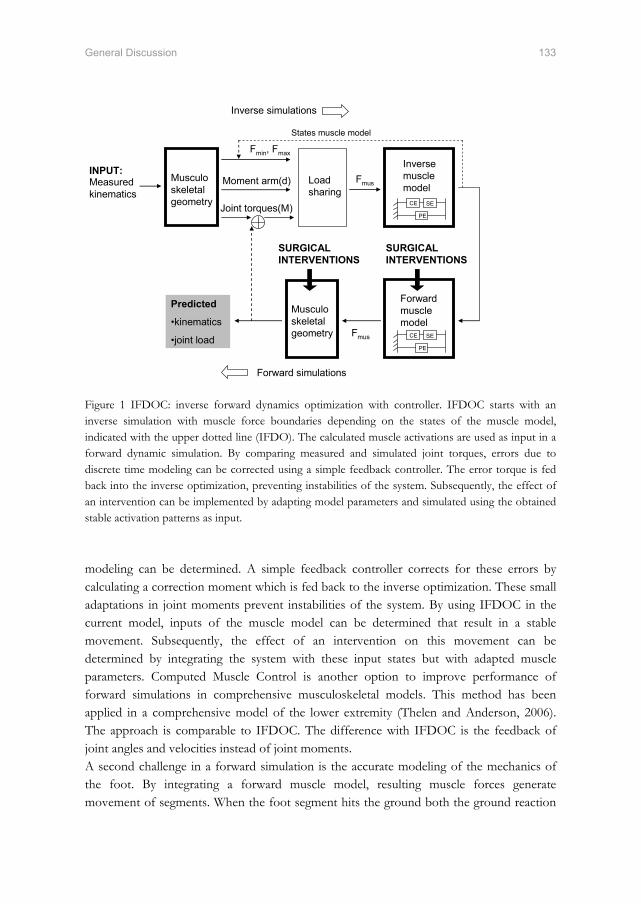
General Discussion 133
Musculo skeletal geometry
Load sharing
Inverse muscle model
Moment arm(d)Measured kinematics
Joint torques(M)
Fmus
Fmin, Fmax
Predicted
•kinematics
•joint load
Forward simulations
Inverse simulations
Musculo skeletal geometry
Forward muscle model
Fmus
States muscle model
CE SE
PE
CE SE
PE
INPUT:
SURGICAL INTERVENTIONS
SURGICAL INTERVENTIONS
Figure 1 IFDOC: inverse forward dynamics optimization with controller. IFDOC starts with an inverse simulation with muscle force boundaries depending on the states of the muscle model, indicated with the upper dotted line (IFDO). The calculated muscle activations are used as input in a forward dynamic simulation. By comparing measured and simulated joint torques, errors due to discrete time modeling can be corrected using a simple feedback controller. The error torque is fed back into the inverse optimization, preventing instabilities of the system. Subsequently, the effect of an intervention can be implemented by adapting model parameters and simulated using the obtained stable activation patterns as input. modeling can be determined. A simple feedback controller corrects for these errors by calculating a correction moment which is fed back to the inverse optimization. These small adaptations in joint moments prevent instabilities of the system. By using IFDOC in the current model, inputs of the muscle model can be determined that result in a stable movement. Subsequently, the effect of an intervention on this movement can be determined by integrating the system with these input states but with adapted muscle parameters. Computed Muscle Control is another option to improve performance of forward simulations in comprehensive musculoskeletal models. This method has been applied in a comprehensive model of the lower extremity (Thelen and Anderson, 2006). The approach is comparable to IFDOC. The difference with IFDOC is the feedback of joint angles and velocities instead of joint moments. A second challenge in a forward simulation is the accurate modeling of the mechanics of the foot. By integrating a forward muscle model, resulting muscle forces generate movement of segments. When the foot segment hits the ground both the ground reaction

134 Chapter 7
force as the deformation of the foot should be accurately described. The ground reaction force affects the torques with respect to the joints and thus the movement of these joints. The deformation of the foot affects the position of the ankle and the other, more proximal joints. Inaccuracies in joint positions and joint torques result in instabilities in the system hampering a successful clinical application. To accurately describe the deformation of the foot and the resulting position of the ankle, a sophisticated foot model is required. Thelen et al. (2006) used springs and dampers under the foot to fit simulated with measured ground reaction force. Yet, to predict the movement of a patient after surgery, experimental data cannot be used as these are not available. Therefore the interaction of the foot with the floor should be modeled very accurately. Incorrect predictions of ground reaction forces result in deviations in joint torques and subsequent movement of the segments. A subject-specific foot model that fulfills these requirements does not exist. The development of a model that accurately describes the interactions of the many bones and passive and active structures requires a major effort with probably a long way to go. In the meantime forward simulations of comprehensive musculoskeletal models are only possible by tracking experimental data. The effects of ligaments were excluded in the inverse dynamic optimization since small errors in joint parameters, joint angles and location of attachment sites of ligaments will cause unrealistically high forces in ligaments and consequently unrealistically high muscle forces. Yet, in a forward dynamic optimization the ligaments of the hip knee and ankle as measured in the dissection study (Chapter 2) can be included in the cost function of the optimization affecting the movement such that the forces in the ligaments are minimal.
7.4.4 Clinical model application
This study aimed to develop a musculoskeletal model which can be used for evaluation of if-then scenarios with respect to the treatment of gait disorders. In the clinical case study in chapter 6 a first step was taken to apply the TLEM for this purpose. The study aimed to relate deformations of the femur observed in myelomeningocele patients with abnormal hip compression forces. A better insight in the cause of these deformations would improve orthopedic treatment. Although a direct relation could not be determined yet, this study was the first that reports hip compression forces in myelomeningocele patients. A comparison with healthy children showed that joint torques and compression forces are different and abnormal in the patients. This study clarified next steps for improvements of the TLEM. The success of a subject-specific model application is highly dependent on the scaling of the model parameters. The more divergent a subject, the more variables should be included in the scaling routine. The generic model as presented allows investigation of many clinical issues. Several projects have already been initiated: To estimate the risk of fractures of a metastasized femur in bone cancer patient a finite element model of the femur is developed based on CT data. The current model can be used to estimate femur

General Discussion 135
loads in activities of daily living. In another study new tendon transfer techniques are simulated to evaluate whether deficiencies in hip abductors torques after hip transplantation can be compensated. The study aims to improve treatment methods and prevent instable hips in these patients after transplantation. Much effort is spent on ambulatory measurement of kinematics of a subject using inertial sensors and force shoes (e.g. (Roetenberg et al., 2007, Schepers et al., 2007)). Accurate ambulatory kinematic data of a subject open many other fields of application of the TLEM. For example, to develop an ergonomic deliberate working environment by estimating peak joint compression forces during a working day.
7.5 Concluding remarks
This study presented a consistent comprehensive musculoskeletal model of the lower extremity. The added value is that the discretization of the human locomotor apparatus is more extensive and more accurate since errors due to merging of datasets are omitted.
Moment arm and maximal isometric moments are in agreement with the literature. Therefore model geometry and force generating properties are considered trustworthy.
A morphological muscle model is required to describe the complex deformations in soleus and knee extensors.
A novel muscle force optimization approach was used, resulting in more realistic muscle synergies. Results are in agreement with EMG and in vivo measured hip compression forces.
More consistent datasets are required to obtain scaling regression equations that relate externally measurable variables with internal variables. This will allow accurate scaling of the model to a subject, which is a condition for a successful application in a clinical practice.

136 Chapter 7
7.6 References
Anderson, F. C.,Pandy, M. G., 2001. Static and dynamic optimization solutions for gait are practically equivalent. Journal of Biomechanics, 34, 153-61.
Bergmann, G., Deuretzbacher, G., Heller, M., Graichen, F., Rohlmann, A., Strauss, J.,Duda, G. N., 2001. Hip contact forces and gait patterns from routine activities. Journal of Biomechanics, 34, 859-71.
Blemker, S. S.,Delp, S. L., 2005. Three-dimensional representation of complex muscle architectures and geometries. Annals of Biomedical Engineering, 33, 661-73.
Brand, R. A.,Crowinshield, R. D., 1982. A model of lower extremity muscular anatomy. Journal of Biomechanics, 104, 153-161.
Chadwick, E. K.,Van Der Helm, F. C. (2003) Combined inverse/forward dynamic optimization of a large-scale biomechanical model of the shoulder and elbow. International symposium on computer simulation in biomechanics. Sydney.
Crowninshield, R. D.,Brand, R. A., 1981. A physiologically based criterion of muscle force prediction in locomotion. Journal of Biomechanics, 14, 793-801.
D'lima, D. D., Patil, S., Steklov, N., Slamin, J. E.,Colwell, C. W., Jr., 2006. Tibial forces measured in vivo after total knee arthroplasty. Journal of Arthroplasty, 21, 255-62.
Delp, S. L., Anderson, F. C., Arnold, A. S., Loan, J. P., Habib, A., John, C. T., Guendelman, E.,Thelen, D. G., 2007. OpenSim: Open-source software to create and analyse dynamic simulations of movement. IEEE Transactions on Biomedical Engineering, 00014, 1-12.
Delp, S. L., Loan, J. P., Hoy, M. G., Zajac, F. E., Topp, E. L.,Rosen, J. M., 1990. An interactive graphics-based model of the lower extremity to study orthopaedic surgical procedures. IEEE Transactions on Biomedical Engineering, 37, 757-67.
Erdemir, A., Mclean, S., Herzog, W.,Van Den Bogert, A. J., 2007. Model-based estimation of muscle forces exerted during movements. Clinical Biomechanics (Bristol, Avon), 22, 131-54.
Finni, T., Komi, P. V.,Lukkariniemi, J., 1998. Achilles tendon loading during walking: application of a novel optic fiber technique. European Journal of Applied Physiology and Occupational Physiology, 77, 289-91.
Glitsch, U.,Baumann, W., 1997. The three-dimensional determination of internal loads in the lower extremity. Journal of Biomechanics, 30, 1123-31.
Heller, M. O., Bergmann, G., Deuretzbacher, G., Durselen, L., Pohl, M., Claes, L., Haas, N. P.,Duda, G. N., 2001. Musculo-skeletal loading conditions at the hip during walking and stair climbing. Journal of Biomechanics, 34, 883-93.
Higginson, J. S., Zajac, F. E., Neptune, R. R., Kautz, S. A., Burgar, C. G.,Delp, S. L., 2006. Effect of equinus foot placement and intrinsic muscle response on knee extension during stance. Gait and Posture, 23, 32-6.
Hill, A. V., 1938. The heat of shortening and the dynamic constants of muscle. proc. R Soc Lond B, 126, 136-195.
Huijing, P., 1999. Muscular force transmission: a unified, dual or multiple system? A review and some explorative experimental results. Archives of Physiology and Biochemistry, 107, 292-311.
Kaptein, B. L.,Van Der Helm, F. C., 2004. Estimating muscle attachment contours by transforming geometrical bone models. Journal of Biomechanics, 37, 263-73.
General Discussion 137
Klein, P., Mattys, S.,Rooze, M., 1996. Moment arm length variations of selected muscles acting on talocrural and subtalar joints during movement: an in vitro study. Journal of Biomechanics, 29, 21-30.
Lloyd, D. G.,Besier, T. F., 2003. An EMG-driven musculoskeletal model to estimate muscle forces and knee joint moments in vivo. Journal of Biomechanics, 36, 765-76.
Maganaris, C. N., 2001. Force-length characteristics of in vivo human skeletal muscle. Acta Physiologica Scandinavica, 172, 279-85.
Maganaris, C. N., 2003. Force-length characteristics of the in vivo human gastrocnemius muscle. Clinical Anatomy, 16, 215-23.
Manal, K.,Buchanan, T. S., 2004. Subject-Specific estimates of tendon slack length: A numerical method. Journal of applied biomechanics, 20, 195-203.
Murray, W. M., Buchanan, T. S.,Delp, S. L., 2002. Scaling of peak moment arms of elbow muscles with upper extremity bone dimensions. Journal of Biomechanics, 35, 19-26.
Pierrynowski, M. R., 1995. Analytic representation of muscle line of action and geometry, in: Allard, P., Stokes, I. A. F. & Blanchi, J. P. (Eds.) Three-Dimensional Analysis of Human Movement. Human Kinetics, Champaign, IL, pp. 214-256.
Praagman, M., Chadwick, E. K., Van Der Helm, F. C.,Veeger, H. E., 2006. The relationship between two different mechanical cost functions and muscle oxygen consumption. Journal of Biomechanics, 39, 758-65.
Roetenberg, D., Slycke, P. J.,Veltink, P. H., 2007. Ambulatory position and orientation tracking fusing magnetic and inertial sensing. IEEE Transactions on Biomedical Engineering, 54, 883-90.
Schepers, H. M., Koopman, H. F.,Veltink, P. H., 2007. Ambulatory assessment of ankle and foot dynamics. IEEE Trans Biomed Eng, 54, 895-902.
Spoor, C. W.,Van Leeuwen, J. L., 1992. Knee muscle moment arms from MRI and from tendon travel. Journal of Biomechanics, 25, 201-6.
Thelen, D. G.,Anderson, F. C., 2006. Using computed muscle control to generate forward dynamic simulations of human walking from experimental data. Journal of Biomechanics, 39, 1107-15.
Van Der Helm, F. C.,Veenbaas, R., 1991. Modelling the mechanical effect of muscles with large attachment sites: application to the shoulder mechanism. Journal of Biomechanics, 24, 1151-63.
Veeger, H. E., Kreulen, M.,Smeulders, M. J., 2004. Mechanical evaluation of the Pronator Teres rerouting tendon transfer. Journal of Hand Surgery. British Volume, 29, 259-64.
Wickiewicz, T. L., Roy, R. R., Powell, P. L.,Edgerton, V. R., 1983. Muscle architecture of the human lower limb. Clinical Orthopaedics, 275-83.
Willems, M. E.,Huijing, P. A., 1994. Heterogeneity of mean sarcomere length in different fibres: effects on length range of active force production in rat muscle. European Journal of Applied Physiology and Occupational Physiology, 68, 489-96.
Winters, J. M.,Woo, S. L. Y. 1990 Multiple muscle systems, Biomechanics and Movement Organisation, New York, Springer-Verlag.
Yucesoy, C. (2003) Intra-,inter- and extramuscular myofascial force transmission. PhD Thesis, University of Twente, Enschede.

Appendix 139
Appendix
Additional information about the Twente Lower
Extremity Model (TLEM)

140 Appendix
Model structure
The Twente Lower Extremity Model (TLEM) has been programmed in SPACAR. This computer program is based on the finite element method, which is a suitable method for kinematic and dynamic analyses of multibody models (van Soest et al., 1992, van der Helm, 1994). In SPACAR there are three basic elements with predefined mechanical properties: HINGE, TRUSS and MULTINODE. Each element is represented by one or more position nodes and/or orientation nodes. With the coordinates of the nodes the deformation modes of the element are determined. For example the deformation mode of a TRUSS element (figure 1), the elongation ε1 with respect to its initial length l0, is determined with the coordinates of its two position nodes P(x,y,z) and Q(x,y,z):
: 0222
1 )()()( lzzyyxx qpqpqp −−+−+−=ε (1)
z
y
x
P
Q
l0
ε1
P Q Initial position
Deformed position
Figure 1 TRUSS element in the initial position and deformed position. The elongation ε1 is defined by position node P and Q (Jonker, 1988, Van der Helm, 1991). A model is defined as a number of elements that are connected by shared common nodes. The kinematic and dynamic behaviour, described by the equations of motion, is fully determined by the generalised coordinates. If the model is mechanically consistent, the unknown coordinates of the other nodes and deformations can be calculated iteratively based on the generalised coordinates. For inverse calculations, the generalised coordinates are pre-described coordinates and/or deformations. In forward dynamic analyses, driving moments and muscle forces are the input to the model. The TLEM comprises connected elements, each representing the relevant morphological structures of the lower extremity: segments, joints, muscles and ligaments. The parameters of each element were based on one recently measured anatomical dataset for the right leg (Klein Horsman et al., 2007). Parameters for the left lower extremity have been determined

Appendix 141
by mirroring the measured data of the right lower extremity in the mid-sagittal plane, defined by the plane perpendicular to the global z-axis through the midpoint of the right and left anterior iliac spine of the pelvis. Segment coordinate systems were determined as described by the Standardization and Terminology Committee of the International Society of Biomechanics (Wu et al., 2002). The foot and talus coordinate systems were calculated analogous to that for the calcaneus. The segments with their attachment sites and joint parameters were rotated from the ‘measured specimen position’ as measured on the specimen to the so-called ‘initial model position’. This was done by prescribing the required deformation of the generalised coordinates. In the measured specimen position, the hip was externally rotated, the knee extended and the ankle in plantar flexion. In the initial model position the local pelvis coordinate system was aligned with the global reference frame and all the joints were in a neutral position (table 1). Joint angles in this study are presented with respect to the initial model position. In the next paragraphs the different elements in the TLEM will be described in more detail (see for overview figure 2). Table 1 Relative segment angles of right lower extremity in the initial model position calculated with an euler XYZ decomposition (in radians). Segment X Y Z Global/Pelvis 0 0 0 Pelvis/Femur -0.07 0.05 0.00 Femur/Tibia 0.26 -0.61 0.16 Tibia/Talus 0.14 0.59 -0.01 Talus/Foot 0 0 0
Body segments
The TLEM consisted of 12 body segments: HAT (Head, Arms, Trunk), pelvis and right and left femur, patella, tibia, talus and foot. A body segment was modelled as a MULTINODE element representing a rigid body. The mass and the center of mass were assigned to the position node and rotational inertia to the orientation node of the MULTINODE element.
Joints
The segments were connected by a common position node on two MULTINODE elements representing the rotation center. The orientation nodes of both MULTINODE elements were connected to a HINGE element. The two corresponding orientation nodes
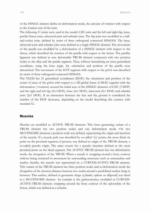
142 Appendix
of the HINGE element define its deformation mode, the amount of rotation with respect to the rotation axis of the joint. The following 11 joints were used in the model: L5S1 joint and the left and right hip, knee, patella/femur joint, talocrural joint and subtalar joint. The hip joint was modelled as a ball-and-socket joint, defined by series of three orthogonal connected HINGES. The knee, talocrural joint and subtalar joint were defined as a single HINGE element. The movement of the patella was modelled by a deformation of a HINGE element with respect to the femur, which described the rotation of the patella with respect to the femur. The patellar ligament was defined as non deformable TRUSS element connected with two position nodes to the tibia and the patella segment. Thus, without introducing an extra generalised coordinate, using the knee angle, the orientation and position of the patella were determined. The movement of the HAT segment with respect to the pelvis was described by series of three orthogonal connected HINGES. The TLEM has 21 generalised coordinates (DOF): the orientation and position of the center of mass of the pelvis with respect to a 3D global frame (6 DOF) together with the deformation (=rotation) around the initial axes of the HINGE elements of L5S1 (3 DOF) and the right and left hip (2x3 DOF), knee (2x1 DOF), talocrural (2x1 DOF) and subtalar joint (2x1 DOF). If an interaction between the feet and the ground is considered the number of the DOF decreases, depending on the model describing this contact, with maximal 12.
Muscles
Muscles are modelled as ACTIVE TRUSS elements. This force generating variant of a TRUSS element has two position nodes and one deformation mode. On two MULTINODE elements a position node was defined, representing the origin and insertion of the muscle. If a muscle path was described by so-called ‘via’ points, the most distal via point on the proximal segment, if present, was defined as origin of the TRUSS element, a so-called pseudo origin. The same counts for a pseudo insertion defined as the most proximal point on the distal segment. The ACTIVE TRUSS element has one deformation mode: the elongation of the TRUSS. When a muscle is wrapping around a bony contour without being restricted in movement by surrounding structures such as retinaculum and tendon sheaths, the muscle was represented by a CURVED-ACTIVE-TRUSS element. This variant of the TRUSS element has three position nodes and as deformation mode the elongation of the shortest distance between two nodes around a predefined surface lying in between. This surface, defined as geometric shape (cylinder, sphere or ellipsoid) was fixed at a MULTINODE element. An example is the gastrocnemius, modelled as CURVED-ACTIVE-TRUSS element, wrapping around the bony contour of the epicondyle of the femur, which was defined as a cylinder.
Appendix 143
Figure 2 The Twente Lower Extremity Model. The upper graphs show pre-scribed joint rotations with respect to 5 DOF of the TLEM (note: total # DOF = 21). In the middle a frontal and side view of the TLEM during the gait cycle. The gray dots represent bony landmarks. Light gray lines are rotation axes. ‘X’ represents the centre of mass of the segments. Only 6 of 264 muscle lines and 1 of the 24 ligaments are showed here. Graphs at the bottom show 4 examples of model outputs for the most proxima1of the 6 muscle elements of the adductor longus. F-l is the normalized force length ratio (at optimal fiber length: F-l = 1). Lmus and Vmus are respectively muscle length and speed divided by the optimal muscle length. Fmus is the optimized muscle force.
144 Appendix
Muscle parameters (muscle mass, pennation angle, Physiological cross-sectional area (PCSA), tendon length and optimal fiber length) were assigned to each ACTIVE TRUSS. To describe the mechanical effect of muscles accurately, some muscles were split up into multiple elements. This was done for muscles with large attachment sites, or with differences in muscle parameters for different muscle parts. The muscle elements were considered as independent actuators. The interaction with the other muscle elements is considered negligible. The resulting model contains 264 ACTIVE TRUSS elements to describe the mechanical effect of 76 muscles of both the lower extremities.
Ligaments
In reality ligaments constrain a movement between two connected segments, restraining the degrees of freedom of a joint. A small length change of a ligament results in large stresses in the ligament. Small errors in joint parameters, measurement of joint angles and location of attachment sites of ligaments will lead to unrealistic high forces in ligaments and consequently in unrealistic high muscle forces in an optimization. Therefore, ligaments were described as non-force-generating TRUSS elements in an inverse dynamic analysis. Model simulations give insight in length change of the ligament during the movement. The model contains 24 truss elements representing ligaments of the hip, knee and ankle of both extremities. In a forward dynamic optimization the mechanical effect of the ligaments will be included in the model. The movement will be affected such that the stress in the ligaments is minimal.
Scaling
The extent and way of scaling varies among different studies and is often underexposed. Many studies used SIMM for definition of musculoskeletal geometry and force generating properties and referred to Delp et al. (1990) (e.g. ((Higginson et al., 2006, Anderson and Pandy, 2001)). However, in Delp’s paper a generic model was presented without scaling routines (Delp et al., 1990). The SIMM 4.0 manual describes different scaling options for musculoskeletal geometry, yet accompanying journal papers are lacking and the selected scaling options are often unmentioned by the users. Furthermore, force generating muscle properties are not scaled according to the SIMM manual. Several scaling assumptions have been reported but vary among different studies. For example Hurwitz et al. (2003) doubled maximal isometric force as defined in SIMM, besides adaptations in some, not further specified, muscle lines of actions (Hurwitz et al., 2003). In another clinical study, 15 unspecified muscles were selected from the total of 43 muscles defined by Delp et al (1990) to span the joints of the leg (Higginson et al., 2006). In that study force generating
Appendix 145
properties were not adapted. In sum, scaling and adaptations in generic anatomical datasets are often unclear. In this paragraph the scaling routines are reported for all the parameters of the TLEM for application to an individual. Finally, some examples are shown to illustrate how model outputs are affected by scaling.
Scaling 1: Inertial properties
Segment mass, center of mass and principal moments of inertia of the subject were calculated using regression equations (Koopman, 1989, Chandler et al., 1975) for the following segments: HAT (head, arms, trunk), pelvis, left and right femur, tibia and foot. The dimensions of the subject’s segments, which are the inputs of the regression equations, were determined using the measured 3D position of the following bony landmarks: sacrum, left and right anterior iliac spine, lateral femur epicondyle, later malleolus, heel and toe.
Scaling 2: Marker tracking
During a gait cycle, marker trajectories were collected that were mounted on the bony landmarks. The bony landmarks as defined in the model were scaled to fit the subject’s bony landmarks in a static standing pose, which defines the neutral joint position. In a dynamic trial joint angles were calculated by optimizing the model markers to fit measured marker trajectories using an approach described by Koopman et al. (1995).
Scaling 3: Musculoskeletal geometry
The musculoskeletal geometry consists of 3D locations of attachment sites of muscles, wrapping surfaces, via points, joint rotation centers. By fitting the bony landmarks to the subject a scaling vector in 3 dimensions can be determined for each of these parameters. The geometrical parameters of a segment, defined as vectors within the local segment frame, were multiplied with the scaling vector for each segment. The radii of wrapping surfaces were scaled using the length ratio of the corresponding segments.
Scaling 4: Force generating parameters
The ratio of the length of a muscle element after and before scaling of the segments was used to scale the corresponding optimal fiber length and tendon length. With the scaled optimal fiber length, the force length relation could be determined. Muscle mass was scaled using the ratio of the total body mass of the subject and the cadaver. The body mass, length ratio for the subject and cadaver were divided and used to scale the PCSA. A specific muscle tension of 45 N/cm2 was used, which agrees reasonably well with the

146 Appendix
literature (Fukunaga et al., 1996). This parameter together with the PCSA defines the amplitude of the isometric force curve. Pennation angle was not scaled.
Examples: effect of scaling on model outputs
The TLEM is based on a male specimen with a total weight of 105 kg and length of 1.74 m. Some examples are shown below (figure 3) to illustrate how model outputs are affected by scaling. The kinematic data of the gait cycle are measured on a healthy subject of 85 kg and length of 1.85 m, as described in chapter 5.
% of gait cycle
Hip
flex
ion
( ← )
/ ext
ensi
on ( →
) to
rque
(Nm
)
10 20 30 40 50 60 70 80 90 100-80
-60
-40
-20
0
20
40
60TLEM scaledTLEM unscaled
% of gait cycle
Bic
eps
Fem
oris
For
ce (N
)
10 20 30 40 50 60 70 80 90 1000
50
100
150
200
250
300TLEM scaledTLEM unscaled
Figure 3 Example of the effect of scaling of segment length. The solid line shows the hip flexion torque during the gait cycle based on segment lengths that fit with the subject. The dotted line shows the torques when the segment length is unscaled. Besides the amplitude, scaling affects the shape of the torque curve and the part of the gait cycle where joint torque crosses zero, which will affect the outcome of the optimization of muscle force. The graph on the right shows the resulting force in the biceps femoris. This typical example shows the relevance of accurate segment scaling as a small deviation in body length (1.85-1.75 m) results in large differences in peak force muscle force.
% of gait cycle
Hip
flex
ion
( ← )
/ ext
ensi
on ( →
) to
rque
(Nm
)
10 20 30 40 50 60 70 80 90 100-100
-80
-60
-40
-20
0
20
40
60inertial parameters -50%inertial parameters +50%
% of gait cycle
Bic
eps
Fem
oris
forc
e (N
)
10 20 30 40 50 60 70 80 90 1000
50
100
150
200
250
300inertial parameters -50%inertial parameters +50%
Figure 3 A 50% increase (dotted) and 50% decrease (solid) of segment mass and moments of inertia of the subject has a small effect on joint torques and muscle force which is in agreement with previous findings (Reinbolt et al., 2007). This illustrates that subject-specific inertial parameters are of minor interest.

Appendix 147
References
Anderson, F. C.,Pandy, M. G., 2001. Static and dynamic optimization solutions for gait are practically equivalent. Journal of Biomechanics, 34, 153-61.
Chandler, R. F., Clauser, C. E., Mcconville, J. T., Reynolds, H. M.,Young, J. W., 1975. Investigation of inertial properties of the human body. Report DOT HS-801430, National Technical Information Service, Springfield Virginia 22151, USA.
Delp, S. L., Loan, J. P., Hoy, M. G., Zajac, F. E., Topp, E. L.,Rosen, J. M., 1990. An interactive graphics-based model of the lower extremity to study orthopaedic surgical procedures. IEEE Transactions on Biomedical Engineering, 37, 757-67.
Fukunaga, T., Roy, R. R., Shellock, F. G., Hodgson, J. A.,Edgerton, V. R., 1996. Specific tension of human plantar flexors and dorsiflexors. Journal of Applied Physiology, 80, 158-65.
Higginson, J. S., Zajac, F. E., Neptune, R. R., Kautz, S. A., Burgar, C. G.,Delp, S. L., 2006. Effect of equinus foot placement and intrinsic muscle response on knee extension during stance. Gait and Posture, 23, 32-6.
Hurwitz, D. E., Foucher, K. C.,Andriacchi, T. P., 2003. A new parametric approach for modeling hip forces during gait. Journal of Biomechanics, 36, 113-9.
Jonker, B. (1988) A finite element dynamic analysis of flexible spatial mechanisms and manipulators. Ph.D. Thesis, Delft University of Technology.
Klein Horsman, M. D., Koopman, H. F., Van Der Helm, F. C., Prose, L. P.,Veeger, H. E., 2007. Morphological muscle and joint parameters for musculoskeletal modelling of the lower extremity. Clinical Biomechanics (Bristol, Avon), 22, 239-47.
Koopman, B. (1989) The three-dimensional analysis and prediction of human walking. PhD Thesis, University of Twente, Enschede.
Reinbolt, J. A., Haftka, R. T., Chmielewski, T. L.,Fregly, B. J., 2007. Are patient-specific joint and inertial parameters necessary for accurate inverse dynamics analyses of gait? IEEE Transactions on Biomedical Engineering, 54, 782-93.
Van Der Helm, F. C. (1991) The shoulder mechanism, a dynamic approach. Ph.D. Thesis, Delft University of Technology.
Van Der Helm, F. C., 1994. A finite element musculoskeletal model of the shoulder mechanism. Journal of Biomechanics, 27, 551-69.
Van Soest, A. J., Schwab, A. L., Bobbert, M. F.,Van Ingen Schenau, G. J., 1992. SPACAR: a software subroutine package for simulation of the behavior of biomechanical systems. Journal of Biomechanics, 25, 1219-26.
Wu, G., Siegler, S., Allard, P., Kirtley, C., Leardini, A., Rosenbaum, D., Whittle, M., D'lima, D. D., Cristofolini, L., Witte, H., Schmid, O.,Stokes, I., 2002. ISB recommendation on definitions of joint coordinate system of various joints for the reporting of human joint motion--part I: ankle, hip, and spine. International Society of Biomechanics. Journal of Biomechanics, 35, 543-8.


Summary 149
Summary
Orthopedic interventions such as tendon transfers have shown to be successful in the treatment of gait disorders. Still, in many cases dysfunctions remained or worsened. To assist clinicians, an interactive tool will be useful that allows evaluation of if-then scenarios with respect to treatment methods. Comprehensive musculoskeletal models have shown a high potential to serve as such a tool. By varying anatomical model parameters, alterations in anatomy due to surgery can be implemented. Inverse and forward model simulations will provide insight in how respectively movement and muscle activations are affected by surgery. Yet, a successful application in clinical practice is hampered due to several shortcomings in existing models. The output of a model is highly dependent on its anatomical model parameters. Two shortcomings can be distinguished in the currently available anatomical datasets. Firstly, existing models were constructed by merging incomplete datasets and estimating missing parameters. This was done in such a way that model outputs fit with in vivo experimental data. Although this may be functional, it is not necessarily an accurate representation. The combined datasets result in an anatomical configuration that never existed. Unknown interactions between different anatomical parameters are lost and resulting errors and inconsistencies are inevitable. Secondly, existing datasets are inaccurate at crucial points. In reality muscles curve around intervening structures, which will affect the line of action of the muscle. In existing datasets many muscles are defined with only one straight muscle element. This is an insufficiently accurate discretization of the musculoskeletal system which has a large effect on model outputs such as muscle force. For example for the equilibration of joints torques in joints with multiple degrees of freedom in reality only certain parts of a muscle may be activated in order to avoid unwanted joint torques. These differentiations within a muscle are not represented with only 1 muscle element, resulting in an unrealistic estimation of muscle force. Besides anatomical parameters, the optimization of muscle force to deal with the redundancy of the musculoskeletal system has several shortcomings. Many models exclude muscle dynamics in the optimization resulting in unrealistic fast transitions in muscle force. Secondly, the relation between the load sharing and the used cost functions is not proven. Many cost functions are only based on muscle force or stress, which excludes the contribution of smaller muscles. This results in unrealistic muscle synergies. The goal of this study is to develop and validate a comprehensive inverse-forward dynamic musculoskeletal model of the lower extremity based on an accurate and consistent anatomical dataset aiming to evaluate if-then scenarios with respect to the treatment of gait disorders. This project started with the collection of a complete and consistent anatomical dataset, containing the orientations of joints (hip, knee, ankle and subtalar joints), muscle
150 Summary
parameters (optimum length, physiological cross sectional area), and geometrical parameters (attachment sites, ‘via’ points, bony contours). One lower extremity, taken from a male embalmed specimen, was studied. Position and geometry were measured with a 3D-digitizer. Optotrak was used for measurement of rotation axes of joints. Sarcomere length was measured by laser diffraction. A total of 38 muscles were measured. Muscles were divided in multiple muscle lines of action based on muscle morphology. 14 Ligaments of the hip, knee and ankle were included. The presented anatomical dataset embraces all necessary data for state of the art musculoskeletal modelling of the lower extremity. Implementation of these data into an (existing) model is likely to significantly improve the estimation of muscle forces and will thus make the use of the model as a clinical tool more feasible. With the collected dataset the Twente Lower Extremity Model (TLEM) was constructed. This two-legged comprehensive musculoskeletal model is described with 21 degrees of freedom (DOF) and contains 10 joints which are crossed by 264 muscle elements. The predictions of the model are highly dependent on the accuracy of the moment arms. Muscle moment arms in the model were calculated as function of the corresponding joint angles and compared with direct measurements in the literature and other musculoskeletal models in order to evaluate the validity of the model geometry. In comparison to other studies, lines of action of the muscles are more extensively represented in the TLEM. The moment arms presented in this study appeared consistent with the relatively wide range of data from the literature (typically 2-3 cm). In general differences were smaller than 2 cm. Since this model is based on accurate measurements of musculoskeletal geometry and its muscle moment arms fall well within the range found in the literature, the representation of muscle line of action can be considered trustworthy. Maximal isometric moments were determined with respect to 6 joint axes of the model based on full activation of all relevant Hill-type muscle elements in the model over the total range of motion. Maximal isometric joint moments calculated over the total range of motion fell within the 95% confidence interval of a number of studies reporting in vivo measured maximal voluntary moments. These comparisons further increased the confidence in the anatomical parameters and the model structure. Yet, for the knee extensors and plantar flexors the reduction of the complex muscle architecture to a Hill model resulted in eminent deviations with in vivo moments. A morphological instead of lumped muscle model is required to describe the complex deformations in these muscles. For the use of the Hill model an adaptation in tendon length was needed to obtain a good fit. As a next step, dynamic properties were added to the TLEM and muscle forces were estimated during gait. Muscle forces were optimized using a novel inverse-forward dynamic optimization (IFDO) algorithm which takes excitation and activation dynamics into account. A recently proposed energy related cost function was utilized, which resulted in a good correspondence with muscle energy consumption. Input joint kinematics during gait were obtained and used as input for the model. Simulations resulted in a stable, fast and

Summary 151
accurate estimation of muscle forces. Measured electromyography (EMG) agreed reasonably well with neural inputs predicted by the TLEM. Estimated joint compression forces were consistent with published in vivo measurements of joint forces; differences were attributed to inter-individual differences in joint torques. This study showed that the effects of model assumptions are eminent. IFDO prevented unrealistic fast transitions in force, which were present in other studies that exclude the effect of excitation and activation dynamics. The energy related cost function induced synergistic muscle activity in which also small muscles participated since muscle mass and fiber length were included as weight factor. This is an improvement when compared to traditional cost functions that are based on muscle force and cross sectional area only. In contrast with other studies, no merging and tuning of anatomical datasets was required to obtain a good fit with EMG and in vivo measured compression forces, which further enhances the reliability of the model predictions. Finally, the TLEM was applied in a clinical case study. Children with myelomeningocele frequently develop (sub-)luxated hip joints due to an increased angle between the neck and the shaft of the femur. More insight in the cause of this deformation would improve treatment methods such as tendon transfers. It was hypothesized that this femur deformation is caused by a more vertically oriented hip compression force in myelomeningocele patients as a result of paralysis of hip abductors. The goal of this study was to investigate if the force patterns on hip after paralysis are in agreement with this hypothesis. Stance and gait were measured with a video system in 4 normal children and 4 children with lower lumbo-sacral myelomeningocele. The measured joint angles were used as model input in order to determine muscle forces, the hip compressive force and the moments on the physis. Externally measurable segment dimensions, medical history and the measured EMG signals were used to scale the model to each individual subject. Results for the normal children were consistent and in agreement with the literature. Myelomeningocele patients showed a reduced hip abduction moment and in some cases even adduction moments during gait. It was shown that by including the patient’s pathological deficiencies in the model, healthy joint torques could not be generated, which is an indication that the patient is forced to walk the deviated Trendelenburg gait due to insufficient abduction torque. Abnormal joint torques resulted in abnormal amplitudes of the compressive force during gait (up to 524 %BW). In general no significant differences in direction of the hip compression force were found between the normal subject and the patients, so the hypothesized cause of the femur neck deformities could not be confirmed. With more extensive scaling routines based on 3D images of bone geometries, femur deformations of a patient can be included in the model. It is expected that this will result in a better scaling of the muscle lines of action such that muscle force and hip compression can be estimated more accurately. This will possibly give more insight in the validity of the hypothesis. This study presented a consistent comprehensive musculoskeletal model of the lower extremity. The added value of this model is that the discretization of the human locomotor

152 Summary
apparatus is more extensive and more accurate since errors due to merging of datasets are omitted. Moment arm and maximal isometric moments were in general in agreement with the literature. Therefore model geometry and force generating properties are considered trustworthy. A novel muscle force optimization approach was used, resulting in realistic muscle synergies. The results were in agreement with EMG and in vivo measured compression force. The collection of more consistent datasets is recommended to obtain scaling regression equations that relate externally measurable variables with internal variables. This will allow accurate scaling of the TLEM to a subject, which is a condition for a successful application in a clinical practice.
Samenvatting 153
Samenvatting
Orthopedische ingrepen zoals peestransposities zijn succesvol gebleken bij de behandeling van loopstoornissen. Toch zijn er ook patiënten bij wie klachten aanbleven of verergerden na een ingreep. Ter ondersteuning van clinici, zou een interactieve ‘tool’ nuttig zijn waarmee if-then scenario’s kunnen worden geëvalueerd met betrekking tot een behandelmethode. Zo kan preoperatief inzicht worden verkregen in het effect van de behandeling. Spierskelet modellen hebben veel potentie voor een dergelijke applicatie. Door anatomische parameters te variëren in een spierskelet model kan een interventie worden gesimuleerd. Inverse en voorwaartse modelsimulaties tonen vervolgens het effect van de ingreep op respectievelijk de activatie patronen van de spieren en de beweging van de patiënt. Door verscheidene beperkingen in de huidige spierskelet modellen is een succesvolle toepassing in de klinische praktijk verhinderd. De uitkomst van een spierskelet model is sterk afhankelijk van de anatomische parameters. De bestaande anatomische datasets hebben 2 tekortkomingen. Ten eerste worden bestaande spierskelet modellen samengesteld door het samenvoegen van verschillende incomplete anatomische datasets en het schatten van ontbrekende parameters. Dit gebeurt zodanig dat een goede fit ontstaat met in vivo experimentele data. Hoewel dit functioneel lijkt, is het niet noodzakelijkerwijs een nauwkeurige representatie van de werkelijkheid. De gecombineerde dataset beschrijft een anatomische configuratie die in werkelijkheid nooit heeft bestaan. Onbekende interacties tussen verschillende parameters zijn verloren en fouten en inconsistenties zijn onvermijdelijk. Een tweede tekortkoming in de bestaande datasets is de onnauwkeurigheid op cruciale punten. Spieren die in werkelijkheid krommen over tussenliggende structuren zijn beschreven als rechte lijn elementen wat resulteert in een onnauwkeurige representatie van de momentsarm ten opzichte van het gewricht. Verder zijn in de huidige datasets veel spieren beschreven met slechts 1 werklijn. Dit is een onvoldoende nauwkeurige discretisatie van het mechanische effect van spieren met grote aanhechtingsoppervlakken. Dit heeft een ongewenst effect op de output van het model. Om bijvoorbeeld gewrichtsmomenten te compenseren rond een gewricht met meerdere vrijheidsgraden kan in werkelijkheid slechts een deel van de spier worden geactiveerd. Deze differentiaties in een spier zijn niet beschreven met slechts 1 spier element, wat resulteert in onrealistische berekening van spierkracht. Naast de anatomische parameters zijn er verscheidene tekortkomingen in de optimalisatie van spierkracht die benodigd is in verband met de redundantie van het systeem. In veel modellen is de dynamica van de spier buiten beschouwing gelaten in de optimalisatie van spierkracht wat resulteert in onrealistisch snelle transities in spierkracht. Verder is er geen bewezen relatie tussen de verdeling van de kracht en de gebruikte optimalisatie criteria.

154 Samenvatting
Veel van deze criteria zijn alleen gebaseerd op spierkracht of spierspanning wat ertoe leidt dat kleine spieren geen kracht leveren. Dit resulteert in onrealistische spier-synergieën. De doelstelling van deze studie is om op basis van een nauwkeurige en consistente dataset een uitgebreid invers-voorwaarts dynamisch spierskelet model van de onderste extremiteit te ontwikkelen en te valideren. De uiteindelijke toepassing van dit model is de evaluatie van if-then scenario’s met betrekking tot de behandeling van loopstoornissen. Dit project is gestart met het vergaren van een complete en consistente dataset op basis van dissectie van een onderste extremiteit van een mannelijk gebalsemd specimen. Deze dataset omvat oriëntaties van gewrichten (heup, knie, enkel en subtalair gewricht), spierparameters (optimale vezellengtes, fysiologische dwarsdoorsnede), en geometrische parameters (aanhechtingsplaatsen, ‘via’ punten, botcontouren). Positie en geometrie zijn gemeten met een 3D-digitiser. Optotrak is gebruikt voor het meten van rotatie-assen van de gewrichten. Sarcomeerlengte is gemeten met behulp van laserdiffractie. In totaal zijn 38 spieren gemeten. Iedere spier is opgedeeld in verschillende spierelementen gebaseerd op verschillen in spiermorfologie. Daarnaast zijn 14 ligamenten van de heup, knie en enkel gemeten. De resulterende dataset bevat alle benodigde data voor de ontwikkeling van een ‘state of the art’ spierskelet model van de onderste extremiteit. Het is waarschijnlijk dat het implementeren van deze data in een (bestaand) model een significante verbetering oplevert spierkracht optimalisatie, benodigd voor een klinische toepassing. Met de gemeten dataset is het ‘Twente Lower Extremity Model’ (TLEM) ontwikkeld. Dit tweebenige uitgebreide spierskelet model van de onderste extremiteit heeft 21 vrijheidsgraden en 10 gewrichten, overspannen door 264 spier elementen. De uitkomst van een spierskelet model is sterk afhankelijk van de momentsarmen van de spieren. De momentsarmen van de spieren in het TLEM zijn berekend als functie van de gewrichtshoeken. Als evaluatie van de validiteit van de geometrie van het model, zijn de momentsarmen vergeleken met directe metingen uit de literatuur en momentsarmen uit andere spierskelet modellen. In vergelijking met andere modellen zijn momentsarmen uitgebreider beschreven in het TLEM. Over het algemeen waren de verschillen met de literatuur kleiner dan 2 cm. De relatief grote spreiding van momentsarmen per spier (typisch 2-3 cm) kan worden toegeschreven aan verschil in meetmethodes en individuen. Omdat het TLEM gebaseerd is op nauwkeurig gemeten anatomische parameters en goed binnen de range van momentsarmen in de literatuur valt wordt de representatie van de werklijnen van de spieren beschouwd als betrouwbaar. Maximale isometrische momenten zijn berekend met het TLEM ten opzichte van 6 gewrichtsassen, gebaseerd op maximale activatie van de desbetreffende Hill spier elementen. De momenten, berekend over het totale bewegingsbereik, vielen binnen het 95% betrouwbaarheidsinterval van in vivo gemeten momenten bij maximale voluntaire contractie, zoals gerapporteerd in een aantal studies in de literatuur. Deze resultaten vergroten de betrouwbaarheid van het model en de bijbehorende anatomische parameters. Hoewel de reductie van de complexe spier architectuur van de knie extensoren en plantair flexoren naar een Hill model tot aanzienlijke verschillen met in vivo momenten heeft

Samenvatting 155
geleid. Een morfologisch model is nodig om de complexe vervormingen in deze spieren te beschrijven. Voor het gebruik van het Hill model was een aanpassing nodig in de peeslengte om een goede fit te krijgen. In een volgende stap in de ontwikkeling zijn dynamische eigenschappen aan het TLEM toegevoegd. Spierkrachten zijn geoptimaliseerd tijdens het lopen met een invers-voorwaarts dynamisch optimalisatie (IFDO) algoritme wat rekening houdt met excitatie en activatie dynamica. Hierbij is een recentelijk ontwikkelt energie gerelateerd criterium gebruikt, die goed overeenstemt met energie consumptie van de spier. Gewrichtshoeken zijn gemeten en gebruikt als input voor het model. De resulterende simulaties waren stabiel, snel en nauwkeurig. Gemeten elektromyografie (EMG) was in goede overeenstemming met de door het model berekende neurale input van verscheidene spieren. Geoptimaliseerde compressiekracht in de gewrichten correspondeerden met in vivo gemeten gewrichtskrachten. Verschillen kunnen worden toegekend aan inter-individuele verschillen in gewrichtsmomenten. Deze studie heeft laten zien dat verschillen door het effect van model aannames aanzienlijk zijn. IFDO voorkomt onrealistisch snelle overgangen in spierkracht die optreden in andere modellen waarbij het effect van spierdynamica buiten beschouwing wordt gelaten. In het energie gerelateerde optimalisatie criterium worden spiermassa en vezellengte gewogen wat leidt tot meer realistische spiersynergieën waaraan ook kleinere spieren deelnemen. Dit is een verbetering in vergelijking met traditionele optimalisatie criteria die slechts gebaseerd zijn op spierkracht en fysiologische dwarsdoorsnede. In tegenstelling tot andere modellen was het in de ontwikkeling van het TLEM niet nodig verschillende datasets samen te voegen om een goede fit met EMG en compressiekracht te krijgen. Dit vergroot de betrouwbaarheid van de voorspellingen van het model. Tot slot is het TLEM toegepast in een klinische studie. Kinderen met myelomeningocele ontwikkelen (sub-)luxaties in het het heupgewricht ten gevolge van een toename van de hoek tussen de nek en schacht van het femur. Meer inzicht in de oorzaak van deze vervormingen zou behandelmethodes zoals peestransposities verbeteren. Er is een hypothese gesteld dat deze deformaties in myelomeningocele patiënten worden veroorzaakt door meer verticaal georiënteerde heup compressiekrachten als gevolg van verlamming van heupabductoren. Het doel van deze studie was om te bepalen of de krachtpatronen op de heup na verlamming in overeenstemming zijn met deze hypothese. Stand en de gang van 4 gezonde en 4 lage lumbo-sacrale myelomeningocele was gemeten met behulp van een optisch video systeem en 2 krachtplaten. De gemeten gewrichtshoeken en externe grondreactiekrachten waren gebruikt als input van het TLEM voor het optimaliseren van spierkrachten en het berekenen van gewricht compressiekrachten en momenten op de physis. Extern meetbare segment dimensies, medische geschiedenis en gemeten EMG signalen waren gebruikt om het TLEM te schalen naar iedere afzonderlijke proefpersoon. Resultaten voor de gezonde proefpersonen waren consistent en in overeenstemming met de literatuur. Myelomeningocele patiënten vertoonden een verminderd heup abductiemoment en in sommige gevallen zelfs een adductiemoment tijdens lopen. Deze

156 Samenvatting
studie heeft aangetoond dat wanneer de pathologische deficiënties van de patiënt worden opgenomen in het model, gezonde gewrichtsmomenten niet geleverd kunnen worden. Dit is een indicatie dat deze patiënten gedwongen worden tot de afwijkende Trendelenburg gang door een verminderd heupabductie moment. Abnormale gewrichtsmomenten resulteerden in abnormale amplitudes van de compressiekrachten in het heupgewricht (tot 524 %BW). Er was geen significant verschil aangetroffen in de richting van de heup compressiekracht in vergelijking met de gezonde proefpersonen, waardoor de hypothese niet kon worden bevestigd. Met meer uitgebreide schalingsroutines gebaseerd op 3D afbeeldingen van het femur, kunnen de deformaties in het bot worden meegenomen in het model. De verwachting is dat dit zal leiden tot een betere schaling van werklijnen van de spieren zodat de spierkrachten en de heup compressiekracht beter kan worden bepaald. Dit zal waarschijnlijk meer inzicht geven in de validiteit van de hypothese. In de huidige studie is een consistent en uitgebreid spierskelet model van de onderste extremiteit gepresenteerd. De toegevoegde waarde ten opzichte van andere modellen is de uitgebreidere en nauwkeurige discretisatie van het menselijke bewegingsapparaat waarbij fouten door samenvoeging van anatomische datasets zijn uitgesloten. Momentsarmen en maximale isometrische momenten in het model zijn over het algemeen in overeenstemming met de literatuur. Daarom worden de modelgeometrie en de krachtseigenschappen betrouwbaar geacht. Er is een nieuwe methode toegepast om spierkracht te optimaliseren wat resulteerde in realistische spier synergieën. De resultaten waren in overeenstemming met EMG en in vivo metingen van compressiekrachten in de heup. Het meten van meer consistente datasets is aanbevolen zodat op basis van uitgebreide regressie vergelijkingen extern meetbare variabelen kunnen worden gerelateerd aan interne anatomische parameters. Dit zal leiden tot een nauwkeurigere schaling van het model, een belangrijke stap richting een succesvolle toepassing in de kliniek.

Dankwoord 157
Dankwoord
Lezen, plannen, meten, programmeren, simuleren, analyseren, opnieuw doorrekenen, schrijven, herschrijven….Na 4 jaar werken zit het erop: Mijn proefschrift is klaar! In dit slotwoord mijn dank aan de mensen die een bijdrage hebben geleverd aan de totstandkoming van dit boekwerk. Allereerst wil ik mijn promotoren Frans van der Helm en Bart Koopman bedanken voor de goede begeleiding. Frans, ik heb het getroffen met een begeleider die zoveel ervaring heeft met het modelleren van het bewegingsapparaat. De besprekingen die we om de twee weken hadden, zorgden iedere keer voor nieuwe motivatie en inspiratie. Je vertouwen in dit project en je grote gedrevenheid hebben mijzelf en dit onderzoek goed gedaan. Bart, het feit dat je altijd in de buurt was en open stond voor vragen heeft gezorgd voor nieuwe impulsen als het even niet liep. Je vermogen om problemen op te lossen of soms gewoon te relativeren, zijn voor mij belangrijke richtingaanwijzers geweest bij het schrijven van dit proefschrift. En er was meer dan werken alleen: Beierse oktoberfesten in augustus, New York Yankees vs. Indians in Cleveland, het eten van gebakken kikkers eten in Taipei… Heren, het was mij een waar genoegen. DirkJan Veeger heeft vanuit de Vrije Universiteit in Amsterdam een belangrijke bijdrage geleverd aan mijn onderzoek. DirkJan, ik heb veel van je geleerd in de maanden dat ik aan het meten was op de snijzaal. Daarnaast heb je door je heldere en kritische blik een verdiepende bijdrage geleverd aan de artikelen in dit proefschrift. Het was een goede en leuke samenwerking, bedankt. Lucian Poliacu Prosé heeft mij de kneepjes van het dissectie vak bijgebracht. Als werktuigbouwkundige tussen chirurgen en anatomen was ik erg blij met iemand die werkelijk ieder vezeltje en ligamentje bij voor en achternaam wist te benoemen. Frans en Erick, de technische stafleden van de snijzaal, hebben gezorgd voor praktische ondersteuning bij bijzondere meetopstellingen. Collega’s van de vakgroep wil ik bedanken voor praktische hulp en gezelligheid tijdens koffiepauzes, borrels, uitjes, sportuitspattingen en congressen. Paul van Geffen heeft als kamergenoot gezorgd voor de mental support bij de laatste loodjes. Het was goed vertoeven in kamer W-205 en W-213, bedankt voor de hulp en de gezelligheid, met als hoogtepunt onze trip naar Taiwan natuurlijk! En niet te vergeten Bart Verdaasdonk en Miguel Aznar Alonso, mijn roommates in de eerste 2 jaar van mijn promotie. Maestro’s, het was een leuke tijd!

158 Dankwoord
Hoewel ik meerdere studenten heb begeleid, wil ik Vera Bulsink en Marieke van Gemert in het bijzonder bedanken voor de directe bijdrage aan dit proefschrift. Vera heeft de Vicon metingen uitgevoerd zoals beschreven in hoofdstuk 4 en Marieke heeft gewerkt aan de eerste klinische toepassing van het model. Dit werk is terug te vinden in hoofdstuk 6. Mijn paranimfen Bram Zuur en Govertjan de With wil ik bedanken voor de ondersteuning tijdens de verdediging. Zowel soulmates als biomedisch ingenieur, ik had geen betere paranimfen kunnen wensen. Lieve (schoon)familie en vrienden, de momenten samen zijn voor mij erg waardevol. Ik voel me vereerd met zulke gave mensen om me heen! In het bijzonder wil ik mijn ouders bedanken. Pap en Mam, hoewel jullie bijdrage aan dit proefschrift niet wetenschappelijk is, heeft jullie steun door mijn leven ertoe geleid dat dit werk uit mijn handen kon komen. Tot slot wil ik Geerieke bedanken. Het was behoorlijk bikkelen laatste paar maanden, maar het is gelukt! Bedankt voor je onvoorwaardelijke liefde en steun. Het heeft me geholpen om door te zetten als het tegen zat. Daarnaast ben ik blij dat je in de afgelopen 4 jaar zorgde voor de goede balans tussen werken en ‘inspannende’ ontspanning: Fietsen naar Rome, sjouwen in Nieuw Zeeland, jungle tracks in Thailand, het was prachtig. Op de fiets naar Nepal zat er niet in, die houd je nog te goed ☺. Lieve Geerieke, ik zie met veel plezier uit naar onze verdere levensreis. Bedankt!
About the Author 159
About the Author
Martijn Klein Horsman was born in Rijssen, the Netherlands, in 1979. His school education started at primary school ‘De Driemaster’ in Hasselt from 1983 to 1991. Subsequently, he went to the ‘Carolus Clusius College’ in Zwolle in 1991, where he received in 1997 his certificate for ‘preporatory scientific education’ (VWO). In the period from 1997 to 2003 he studied Mechanical Engineering at the University of Twente. The subject of his Msc thesis was ‘the estimation of body segment orientation using inertial sensing’. This research was done at Roessingh Research and Development, Enschede with prof. dr. Frans van der Helm as supervisor. In 2003 he was employed as PhD student at the Biomedical Engineering group at the faculty of Engineering Technology of the University of Twente. This research was conducted under supervision of prof. dr. Frans van der Helm and prof. dr. ir. Bart Koopman. His research concerns the musculoskeletal modeling of the lower extremity aiming to assist in the treatment of gait disorders. The present thesis is the result of this study. January 2008, Martijn will start with a new challenge in Canada, where he will be working as postdoctoral researcher in the Human Performance Laboratory at the University of Calgary.
