The Treatment of Long-Wave Radiation and Precipitation in Climate Files forBuilding Physics Simulations

Petter Wallentén, PhD

ABSTRACT

There is an increased demand for hourly heat and moisture simulations for buildings. In simulation programs aimed at energycalculations, it has been enough to include the parameters: temperature, relative humidity, solar radiation, wind speed, wind direc-tion, and cloud cover (Crawley et al. 1999; Wilcox and Marion 2008). These parameters are often a mix of measured and calculateddata. Long-wave radiation from the sky and precipitation are sometimes used as parameters but are not as frequently measured.When focusing on horizontal or tilted surfaces, long-wave radiation can not be neglected. In most climate files, the long-waveradiation is not present, so the simulation programs have to make an educated guess based on available parameters. One importantsecondary parameter is cloudiness, which is measured or calculated from solar radiation compared to maximal theoretic solarradiation. Precipitation is necessary when making moisture calculations for the building envelope. The precipitation is oftenmeasured every 6th or 12th hour, so the simulation programs must distribute this over a period hours in between. This paper pres-ents some of the techniques for these calculations and compares the results with real, hourly measured data for four locationsin Sweden. General results are that the existing investigated models for long-wave radiation give a root-mean-square accuracybetween 24–27 W/m2 and that the models for Sweden using parameters identified above give a root-mean-square error up to23.2 W/m2. For precipitation, the optimal hourly limit value for precipitation was 88% RHc.

INTRODUCTION

When calculating temperature and moisture for build-ings, some kind of hourly climate file must be used. The twomost obvious possibilities are to use measured data from aspecific location or constructed data as a base for the climatefile. The constructed data can be, for example, hourly valuesfor a typical year or a design (worst case) year for a location.In any case, the climate data must be based on measurements.Meteorological stations usually measure temperature, mois-ture content (measured as dew point or relative humidity),pressure, wind speed, and wind direction on an hourly basis.Precipitation and cloud cover are often measured moreseldom; for example, cloud cover is measured every three andprecipitation every twelve hours or daily (SMHI 1988).Global and diffuse solar radiation are measured in fewer loca-tions. If the solar parameters are not measured, they must be

modeled from latitude, cloud cover, etc. (Meyers and Dale1983; Atwater et al. 1978). Note that there are, of course, largedifferences between countries and locations; the airports willalways have climate stations but do not necessarily have auto-matic hourly stations. Temperature calculations for walls andwindows can, in most cases, be made based on this data withreasonable accuracy. The sky temperature for these verticalcases typically is set equal to the air temperature minusaround 10°C. For tilted or horizontal surfaces (roofs, glazedspaces, etc.) the calculations must also include the detailedlong-wave thermal radiation from the sky to be accurate (Wall1996). However, the long-wave radiation from the sky is oftennot measured at all. The reason for this is probably that theprice of the measuring instrument has been higher than theexpected use of the data. For moisture calculations, hourlyvalues for precipitations are needed. This paper investigates

© 2010 ASHRAE.

P. Wallentén is a senior lecturer in the Department of Building Physics, Lund University, Lund, Sweden.

some existing techniques for constructing hourly values forlong-wave radiation and precipitation.

LONG-WAVE RADIATION

Long-wave radiation from the sky (Lw) is typicallymeasured in W/m2 or W·h/m2·h. The measuring instrument issome kind of pyrgeometer, e.g., a Hukseflux IR02 with anaccuracy of 10% for daily sums (Hukseflux manual). To makeit clear that this radiation does not originate from the sun, it issometimes called the atmospheric long-wave radiation. Thelong-wave radiation is in the order of 200–400 W/m2 (Flerch-inger et al. 2009; Crawford and Duchon 1999) and varies ona daily and seasonal basis (see Figure 1).

When formulating algorithms based on other meteoro-logical data, it is natural to start with the Stefan-Boltzmannequation for thermal radiation from a surface with tempera-ture T (K):

(1)

where ε is the emissivity of the surface and σ is the Stefan-Boltzmann constant. Many authors have formulated algo-rithms for Lw mainly based on

• outdoor temperature To (K);

• moisture content in air described by outdoor vapor pres-sure eo (kPa), dewpoint Td (K), or precipitable water w(mm);

• some kind of cloudiness index, cx (dimensionless); and

• atmospheric pressure at the ground (more seldom).

Clear Sky

It is natural to start by deriving algorithms for clear-skyconditions. The clear sky gives a more stable long-wave radi-ation and is of special interest when the minimum long-waveradiation is the key parameter. Given the parameters in Equa-tion 1, one possible choice is to use the outdoor temperature Toas T in Equation 1 and have ε dependent on the other measuredparameters. Examples of this are Equations 3–5:

(2)

Ångström (1918):

(3)

Berdahl and Martin (1984):

(4)

Niemelä et al. (2001)

(5)

Here Td is the dewpoint temperature (°C), eo is the vaporpressure (kPa), and Lw,clr is the long-wave radiation from aclear sky. The Ångström equation is as cited by Flerchinger etal. (2009). Another possibility is to have Lw,clr dependent onthe parameters directly.

Dilley and O’Brien (1998):

(6)

with w as the precipitable water in millimeters.

(7)

Cloudy Sky

For hourly calculations in the context of buildings, thecloudy skies must also be accounted for. If the cloudiness issomehow directly measured, this value is of course to be used.If however the solar radiation is measured but not the cloudi-ness, the cloudiness can be calculated from the measured mete-orological data, e.g., global solar radiation, direct solarradiation, or diffuse solar radiation. Solar data is only availableduring daylight hours so some strategy must be chosen for howto handle the whole day, e.g., a moving twenty-four-hour aver-age or an average of a few hours close to sunset and sunrise.Since the calculated cloudiness should describe the whole sky,it is natural to choose the global solar radiation. The algorithmsbelow for calculating the cloudiness use either the theoreticalextraterrestrial global solar radiation on a surface parallel to theEarth’s surface outside the atmosphere H0 (Wh/m2·h) or the

Figure 1 Measured long-wave radiation from Lund (May14, 1995 to May 21, 1995).

Lw ε σ T4⋅⋅=

Lw clr, εclr eo To …, ,( ) σ To4⋅⋅=

εclr 0.83 0.18– 10 0.067eo–⋅=

εclr 0.738 0.61Td

100---------⎝ ⎠

⎛ ⎞ 0.20Td

100---------⎝ ⎠

⎛ ⎞2

+ +=

εclr

0.72 0.09 eo 2–( )+ , eo 0.2≥ ,

0.72 0.76 eo 2–( )– , eo 0.2<⎩⎨⎧

=

Lw clr, 59.38 113.7To

273.16----------------⎝ ⎠

⎛ ⎞6

96.96 w25------+ +=

w 4650eo

To-----=

2 Buildings XI

theoretical global solar radiation on the Earth’s surface S0 (W/m2·h). The formula for the extraterrestrial radiation takes intoaccount the varying distance from sun to Earth, as well as thedeclination (El-Sebaii et al. 2010). In this paper, H0 is the dailyaverage extraterrestrial radiation (Wh/m2h):

(8)

where ϕ (rad) is the latitude, δ (rad) is the solar declination, ωs(rad) is the sunset hour angle, ISC is the solar constant (1367Wh/m2h), and dnr is the day number (1–365).

(9)

(10)

The clearness index K0 (dimensionless) is defined as thequota between the measured global solar radiation on a hori-zontal surface on the ground IG (W·h/m2·h) and the extrater-restrial solar radiation H0.

(11)

Since the clearness index is the quota of two different enti-ties, the actual cloud cover is not obviously linear dependenton K0. The cloud cover c (dimensionless) is a value between0 and 1 that describes the fraction of the sky that is covered byclouds. According to Flerchinger et al. (2009) c can be calcu-lated as c = 0 for K0 > kclr and c = 1 for K0 < kcld and linearlyinterpolated in between. The values for

and

were investigated in detail by Flerchinger et al. (2009).An index describing the cloud cover can also be based on

theoretic global solar radiation on the Earth’s surface S0 (W·h/m2·h). The solar index s (dimensionless) is defined as thequota between the measured global solar irradiance IG and thetheoretical value S0 (Flerchiner et al. 2009; Crawford andDuchon 1999):

(12)

This is, however, much more complicated than calculat-ing the extraterrestrial radiation, since the influence of theatmosphere must be taken into account. This includes thelength of the solar rays in the atmosphere (air mass), Rayleighscattering, aerosol extinction, water vapor absorption, andpermanent gas absorption. Numerous models exists to

describe these phenomena Yang et al. (2006), Atwater andBall (1978), Meyers and Dale (1983), López et al. (2007).Some are based on physical interpretations and some are moredirect parameter fitting. Flerchinger et al. (2009) used aformula presented by Crawford and Duchon (1999) that wasan adaptation of a formula presented by Atwater and Ball(1978). We will present the model from Crawford as presentedby Flerchinger to calculate S0 for every hour:

(13)

where τR, τpg, τw, and τa denote the transmission coefficientsfor Rayleigh scattering, absorption by permanent gases,absorption by water vapor, and absorption and scattering byaerosols, respectively. The parameter h is the height of the sunover the horizon (solar altitude). The product of Rayleigh scat-tering and absorption by water vapor was calculated asfollows:

(14)

Here m is the optical air mass at 101.3 (kPa) and P is thepressure (kPa). The air mass can be calculated with differentformulas of increasing complexity and accuracy. Atwater andBall (1978) and, successively, Crawford and Duchon (1999)and Flerchinger et al. (2009), calculated m as (even if theformula itself is erroneously described by Crawford andDuchon and Flerchinger et al):

(15)

A more accurate formulae from Young (1994) (originallyexpressed in zenith angle) is

(16)

Young claims this formula has an error less than 0.0037air masses close to the horizon, where the air mass is 31.7. Theformula from Atwater and Ball gives an air mass at the horizonof 35.

The transmission coefficient for absorption in water τw isfrom Flerchinger et al. (2009)

(17)

where w is the precipitable water (mm). The transmissioncoefficient for aerosol extinction τa is from Meyers and Dale(1983) and, successively, Flerchiner et al.:

(18)

The number 0.935 is very much dependent on the amountof particles in the atmosphere. Another way of expressing τais from Louche et al. (1987):

H0

ISC

π-------- 1 0.033 2π

dnr

365---------⎝ ⎠

⎛ ⎞cos+⋅=

x ϕ( )cos δ( ) ωs( )sincos ωs ϕ( ) δ( )sinsin+( )

δ 0.4093= 2π284 dnr+

365-----------------------⎝ ⎠

⎛ ⎞sin⋅

ωs 1–cos ϕ( ) δ( )tantan–( )=

K0

IG

H0------=

kclr 0.7≈

kcld 0.3≈

SIG

S0-----=

S0 ISC h( )sin τR τpg τw τa⋅⋅⋅⋅=

τR τpg⋅ 1.021 0.084 m 0.00949P 0.051+( )[ ]0.5–=

m 351224 2sin h( ) 1+⋅( )0.5---------------------------------------------------------=

m =

1.002432 2sin h( ) 0.148386 h( )sin 0.0096467+ + 3 h( )sin 0.149864 2sin h( ) 0.0102963 h( )sin 0.000303978+ + +

------------------------------------------------------------------------------------------------------------------------------------------------------------

τw 1 0.077 wm10------⎝ ⎠

⎛ ⎞ 0.3–=

τa 0.935m=

Buildings XI 3

(19)

Here β is the Ångström turbidity. To have a similar behav-ior as Equation 18, the turbidity should be about β = 0.06.Sinus of the solar height can be calculated as

(20)

Equation 13 can be made more accurate to include theEarth’s elliptic path around the sun, as in Equation 8. Theequation then becomes

(21)

In Flerchinger et al., the twenty-four-hour average of S0was used; it was also used in the investigation presented below.With the clearness index K0, the cloud cover c, or the solarindex s it is now possible to formulate long-wave radiationfrom a cloudy sky in many different ways.

Aubinet (1994):

(22)

(23)

Aubinet (1994):

(24)

(25)

In Equation 25, Tcld (K) is the temperature of the cloudcover and, the emissivity is set to 1.0 in Equation 24.

Crawford and Duchon (1999):

(26)

where εclr can be calculated by the different equations above.Flerchinger et al. used Dilley and O’Brien (1998) (Equation 6)with good results.

Kimball et al. (1982):

(27)

Here Tc (K) is the cloud temperature. Flerchinger et al.used Tc = To – 11 K. Obviously, the long-wave radiation Lw,clr

from the clear sky must be calculated by other means. Flerch-inger et al. used the Dillay and O’Brian (1998) formula (Equa-tion 6), which is also used in this paper. They performed aninvestigation of the optimal choices for kclr and kcld for thisformula which gave

(28)

Problem and Hypothesis

The need for long-wave radiation data in Sweden hasincreased since a greater accuracy in energy, temperature, andmoisture calculations is in demand. This data is, however,lacking, except for a few locations, so data must be calculatedfrom equations as described above. The commercial program,Meteonorm, is used by many engineers to produce this databased on Aubinet (1994) (Equation 25). This paper investi-gates three of the existing formulas above (Equations 25–27)as well as six new formulas (Equations 29–34) for reference.These new formulas are formulated from a parameter estima-tion view and not necessarily the physical interpretation. Theequations are described below with denoted names for simplerreference. The hypothesis is that there exists one or moreformula that gives results with acceptable accuracy for thelong-wave radiation. Acceptable accuracy is not exactlydefined—it depends on the particular usage—but since thestated accuracy of one pyrgeometer (Hukseflux) is around10% for daily sum, this indicates an accuracy of 30 W/m2.

For reference, a parameter fit of Equation 25 from (1994)was done:

Aubinet (1994) identified

(29)

Two equations were formulated to test the sensitivity tothe clearness index K0 and the solar index s:

Clearness identified

(30)

Solar index identified

(31)

Note that εcld describes the total emissivity and should beused as in Equation 22. The method of Crawford and Duchon(1999) (Equation 26), together with a parameter fit based onBerdahl and Martin (1984) (Equation 4), gave the following:

Berdahl 1 identified

(32)

τa 0.1082 0.878e 1.60βm–+=

h( )sin ϕ( )sin δ( )sin ϕ( )cos δ( )sinπ t 12–( )

12----------------------⎝ ⎠

⎛ ⎞cos+=

S0 ISC h( )sin 1 0.033 2πdnr

365---------⎝ ⎠

⎛ ⎞cos+ τR τpg τw τa⋅ ⋅⋅⋅=

Lw cld, εcld σ To4⋅⋅=

εcld K0( ) 0.93 0.139 1 K0–( )ln–=

Lw cld, σ Tcld4⋅=

Tcld eo To K0, ,( )

94 12.6 1000eo( )ln 13K0 0.341To+–+=

Lw cld, εcld σ To4⋅⋅=

εcld s( ) 1 s–( ) s+ εclr⋅=

Lw clr, Lclr τ8cf8σ Tc4⋅+=

τs 1 ε8z– 1.4 0.4ε8z–( )=

ε8z 0.24 2.98 10 6– eo2 e

3000To------------

⋅⋅⋅+=

f8 0.6732– 0.6240 10 2– Tc 0.9140 10 5– T2⋅⋅–⋅+=

kclr 0.8=

kcld 0.25=

Tcld eo To K0, ,( ) θ1 θ2 1000eo( )ln θ3K0 θ4T0+ + +=

εcld θ1 θ2

Td

100---------⎝ ⎠

⎛ ⎞ θ3

To

273.15----------------⎝ ⎠

⎛ ⎞ θ4K0+ ++=

εcld θ1 θ2

Td

100---------⎝ ⎠

⎛ ⎞ θ3

To

273.15----------------⎝ ⎠

⎛ ⎞ θ4s+ + +=

εclr θ1 θ2

Td

100---------⎝ ⎠

⎛ ⎞ θ3

Td

100---------⎝ ⎠

⎛ ⎞2

+ +=

4 Buildings XI

During the investigation, the accuracy of was low, soanother equation was also tested:

Berdahl 2 identified

(33)

Finally, a formula based on Crawford and Duchon (1999)(Equation 26) and Dilley and O’Brien (1998) (Equation 6) wastested.

Crawford Dilley identified

(34)

Method

At four locations in Sweden, the hourly long-wave radi-ation, temperature, relative humidity, and global solar irradi-ance have been measured from 1990–1998. Over this period,the equipment has sometimes failed. Two longer periods withvalid data have been chosen for each location. The locationsand the periods are shown in Table 1.

The hourly data have been used to identify the parametersin Equations 29–34 and to verify these identifications. Theidentification was made using multiple linear regressionsbased on the least squares error function:

(35)

Here θ is the parameter vector. The estimate of θ denoted minimizes the error function . The data from Period A

was used for identification, and the data from Period B forverification.

The identification gives

• fitted parameters and• standard deviation σ (%) in the parameter fitting.

The verification gives

• root mean square error RMS, (W·h/m2·h);• mean bias MB (W·h/m2·h) (positive when giving too

high a value); and• regression value r (dimensionless).

Results for Long-Wave Radiation

The results from the verification of Equations 25–29 and theidentification and verification of Equations 29–34 are presentedin Table 2. The RMS MB and r are based on 64 204 hourly values(Table 1, Period A) from the four locations in Sweden, and theidentified parameters θ are based on different 121 924 hourlyvalues (Table 1, Period B)from the same location.

The results in Table 2 for the existing Equation 25, Equa-tions 26 plus Equation 6, and Equation 27 plus Equation 6 aresimilar to the results calculated by Flerchinger et al. (2009),based on seven locations in United States, including Alaska.These values are compared in Table 3.

Given that the long-wave radiation varies between 200–400 Wh/m2·h, the RMS is about 10%. From Tables 2 and 3, itis clear that the equations do not give exceptionally differentresults. The equation that gives the best results is the onedenoted “Clearness Identified,” which uses outdoor (To),dewpoint temperature (Td), and the clearness index (K0) asparameters. The Solar Index identification equation gives aslightly worse result. Of the already existing equations, theKimball et al. (1982) and Dilley and O’Brien (1998) equationsgave a surprisingly similar result (given that there was nofitting to the Swedish climate).

During the analysis of the results, some issues was espe-cially noted:

• There was a tendency for higher latitudes to give a largererror.

• There was a tendency for the estimated global solar irra-diance S0 to be too low for higher latitudes, especiallyfor Luleå at 65.55°, where twenty-four-hour average S0was lower than the 24h average measured global solarirradiance on numerous days.

This led to a more detailed analysis. The simple formula(Equation 15) for calculating air mass reduced S0, comparedto the more exact formula (Equation 16). Close to the horizon,the difference is 35 versus 31.7.

The formula for the aerosol extinction (Equation 18) wasequivalent to an Ångström turbidity of about 0.06. TheÅngström turbidity will strongly affect the global solar irradi-ance, especially for high latitudes (∼55°), where the sun is lowand, consequently, the air mass high. It is a well-known fact

θ2

εclr θ1 θ2

Td

100---------⎝ ⎠

⎛ ⎞ θ3

To

273.15----------------⎝ ⎠

⎛ ⎞2

+ +=

Lw clr, θ1 θ2

To

273.16----------------⎝ ⎠

⎛ ⎞6

θ3w25------+ +=

V θ( ) 12--- Lw measured,

i Lw calculated,i θ( )–( )2

i 1=

N

∑=

θ̂ V θ( )

θ̂

Table 1. Locations and Periods with Valid Data

Location Latitude Period A Period B

Lund 55.72 90.06.18–94.06.05 94.07.09–95.11.29

Stockholm 59.35 92.07.10–95.08.01 95.08.04–98.07.02

Borlänge 60.48 92.11.10–95.10.30 97.08.19–98.11.30

Luleå 65.55 93.03.03–97.01.31 91.05.23–93.02.21

Buildings XI 5

that turbidity varies strongly, with a tendency to be highestclose to the equator (~0.08) and lower at the poles (~0.01),(Yang et al. 2001). The value also has a tendency to be lowerin winter and higher in the summer with a variation of +0.02–0.06 (Yang et al. 2001):

(36)

Here z (m) is the height over water level. Fox (1994) esti-mated the Ångström turbidity for Fairbanks, Alaska, (latitude64.82°) for the longest consecutive period (Table 4). The yearlyturbidity is about 0.04±0.02. It must also be stated that theturbidity did not vary smoothly over all the measured periods.

From these facts, the conclusion was drawn that a turbid-ity equivalent to 0.06 for all locations and periods woulddecrease the global solar radiation too much in Sweden. FromPersson (1999), the turbidity in Lund (latitude 55.72°) wasaround 0.07 and for Kiruna (latitude 67.83°) around 0.045.

Therefore, a dependency on both year and latitude was used tocapture this behavior more strongly than in Equation 36:

(37)

There is a strong tendency that increasing latitude giveslarger error than in Flerchinger et al. (2009). This is also validin this investigation.

The last investigated parameter was the albedo. Theformulas for S0 presented above do not take into account thefact that the Earth’s albedo, which is about 0.2, will reflect partof the global solar irradiance back to the atmosphere where asmaller part will be reflected back down again due to the atmo-sphere albedo, which is about 0.0685 for clear skies, accordingto Atwater and Ball (1978). Atwater and Ball suggested thefollowing formula:

(38)

Table 2. Results from Tested Equations

Equation RMS (MB) r θ (σ %)

Aubinet (1994) (Equation 25) 27.0 (–10.8) 0.861 —

Crawford and Duchon (1999) (Equation 26) + Dilley and O’Brian (1998) (Equation 6) 25.4 (–9.3) 0.878 —

Kimball et al (1982) (Equation 27) + Dilley and O’Brian (1998) (Equation 6) 24.0 (4.8) 0.892 —

Aubinet Identified (Equation 29) 23.4 (–3.9) 0.898

34.17 (9.9)7.18 (4.0)

–21.35 (1.8)0.700 (2.6)

Clearness Identified (Equation 30) 23.2 (–3.0) 0.900

1.547 (0.8)0.598 (0.9)–0.569 (2.2)–0.280 (0.4)

Solar Index Identified (Equation 31) 23.5 (–3.3) 0.897

1.684 (0.7)0.631 (0.9)–0.706 (1.8)–0.194 (0.4)

Berdahl 1 Identified (Equation 32) 23.8 (–3.1) 0.8940.747 (0.04)0.456 (0.8)1.789 (1.8)

Berdahl 2 Identified (Equation 33) 23.5 (–2.7) 0.8981.068 (0.7)0.679 (0.9)–0.294 (2.3)

Crawford Dilley Identified (Equation 34) 23.3 (–2.5) 0.89959.00 (0.8)114.37 (0.6)111.29 (0.8)

Table 3. Comparison between Results from This Investigation and Flerschineg et al. (2009)for Cloudy Skies (W·h/m2·h)

Equation RMS (MB) Sweden RMS (MB) Flerchinger

Aubinet (1994) (Equation 25) 27.0 (–10.8) 30.1 (–15.7)

Crawford and Duchon (1999) (Equation 26) + Dilley and O’Brian (1998) (Equation 6) 25.4 (–9.3) 25.8 (–1.3)

Kimball et al (1982) (Equation 27) + Dilley and O’Brian (1998) (Equation 6) 24.0 (4.8) 26.7 (1.0)

β 0.025 0.1 ϕ( )cos+ e0.7z1000------------⋅ 0.02 0.06–( )±=

β 0.025 0.1 2 ϕ( )cos 0.03 2πdnr

365---------⎝ ⎠

⎛ ⎞cos–⋅+=

S0a S0

11 rsra–------------------=

6 Buildings XI

Here, rs (dimensionless) is the surface (Earth) albedo, ra(dimensionless) is the atmosphere albedo and is globalsolar irradiance corrected for albedo (W·/m2·h). The influenceof the Earth’s albedo is mostly important when there is a snowlayer. The albedo can then be around 0.8–0.9.

In the results shown in Table 2, all the following correc-tions were made in comparison to Flerchinger et al. (2009):

1. improved air mass calculation (Equation 16)2. improved turbidity calculation (Equations 19 and 37)3. albedo (with snow cover during December to February)

(Equation 38)

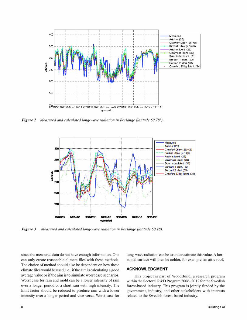
This also explains part of the differences in Table 3.Given all these corrections the equations above do not

give a very accurate reproduction of the long-wave radiationon a detailed level. Figures 2 and 3 show a comparisonbetween the presented formula for 45 days and 5 days, respec-tively, in Borlänge, which shows the variation between theequations.

PRECIPITATION

Precipitation can be measured on an hourly up to a dailybasis in Swedish meteorological stations. It is common tomeasure every 12 h. Blocken and Carmeliet (2008) showed thatto properly model the driving rain on a wall, the hourly drivingrain should be based on nonarithmetic weighted average of 10min measurements of rain and wind. Unfortunately this is notusually available data. Most building simulation programsneed hourly values, so the rain must be distributed over theprevious 12 h by some strategy. Harderup (1988) suggested theuse of hourly relative humidity measurements to do this distri-bution. Other techniques include the use of statistical methods(Günter et al. 2001; Meteonorm handbook). These latter tech-niques are more aimed at hydrological applications and not, forexample, mold estimates in building structures. There is also arisk that purely statistical methods will give conflicting data,for example low humidity and rainfall. As in the case of recon-structing long-wave radiation, it is not possible to accuratelyreconstruct rain based on 12 h values.

Method

Reconstructed hourly values based on 12 h measurementswere compared with hourly measurements from the period ofJanuary 10, 1996 to October 27, 1997 in Stockholm Sweden.The distribution strategy that was chosen was that the hourreceived rain if the relative humidity exceeded a critical valueRHC = 88%. If no hours in the period exceeded this value, thehour with the maximal hour received the rain. This limit valuewas chosen since it maximized the fitted r value or quality of

fit (0.486), as well as minimized the mean absolute hourlyerror (0.0565 mm/h).

Results

Reconstructed and measured hourly data for five days inJune are shown in Figure 4. It is clear that the differencebetween the reconstructed and measured values is high. Thestandard deviation for reconstructed and measured data was:0.198 mm/h and 0.310 mm/h, so the reconstructed data had alower variation, which can be expected given the simplechoice of reconstruction method.

Even if the choice of RHC minimizes the mean absoluteerror, it is not a deep minimum. Table 5 shows the r value andmean absolute error for different choices of RHc.

Figure 5 shows the measured rain versus the relativehumidity. It is clear that the reconstruction of the hourly rain-fall from 12 h values is a crude process at best.

CONCLUSIONS AND DISCUSSION

The long-wave radiation can be calculated from meteo-rological data to an accuracy of about 10%, which, inciden-tally, is the same size as the error reported for a pyrgeometer.The hypothesis that there exists one formula that give the mostaccurate values cannot be fully confirmed in this study. Theexisting formula from Kimball et al. (1982), together withDilley and O’Brian, gave a good fit. This formula has theadvantage of using the extraterrestrial global irradiance asreference, which makes it less sensitive to calculation of airmass and turbidity. For Sweden the best formula was a newformula (Clearness identification), which was similar to theone above since it also used the extraterrestrial global solarirradiance as reference. This formula was, however, muchmore simple. The formula by Aubinet (1994) (Equation 25)gave the worst result and, even when the parameters wereidentified to fit the Swedish data (Equation 29), had the lowestaccuracy. Equation 26, using the global solar irradiance on theEarth surface as a reference, was very sensitive to how the airmass, turbidity, and Earth’s albedo were made, especially forlatitudes above 60°N. For the Equation where the parameterswere identified to the Swedish data, the difference in perfor-mance was remarkably low—almost all had a root-mean-square error close to 23.5 Wh/m2·h.

The reconstruction of rain from 12 h to 1 h values basedon relative humidity gave a crude result, even if the chosenlimit value for the humidity minimized the r value and meanabsolute error. Perhaps estimation of the cloud cover could beincluded to increase accuracy, with the assumption that raindoes not fall from a clear sky.

For the reconstruction of both rain and long-wave radia-tion to hourly values, the “true” values can never be achieved

Table 4. Ångström Turbidity from Fox (1994) for Fairbanks Alaska, Latitude 64.82°

Jan Feb Mar Apr May Jun Jul Aug Sep Oct Nov Dec Annual

0.023 0.024 0.027 0.04 0.059 0.048 0.044 0.028 0.029 0.026 0.027 0.022 0.03

S0a

Buildings XI 7

since the measured data do not have enough information. Onecan only create reasonable climate files with these methods.The choice of method should also be dependent on how theseclimate files would be used, i.e., if the aim is calculating a goodaverage value or if the aim is to simulate worst case scenarios.Worst case for rain and mold can be a lower intensity of rainover a longer period or a short rain with high intensity. Thelimit factor should be reduced to produce rain with a lowerintensity over a longer period and vice versa. Worst case for

long-wave radiation can be to underestimate this value. A hori-zontal surface will then be colder, for example, an attic roof.

ACKNOWLEDGMENT

This project is part of WoodBuild, a research programwithin the Sectoral R&D Program 2006–2012 for the Swedishforest-based industry. This program is jointly funded by thegovernment, industry, and other stakeholders with interestsrelated to the Swedish forest-based industry.

Figure 2 Measured and calculated long-wave radiation in Borlänge (latitude 60.78°).

Figure 3 Measured and calculated long-wave radiation in Borlänge (latitude 60.48).

8 Buildings XI

NOMENCLATURE

β = Ångström turbidity, dimensionlessδ = declination of sun, radε = emissivityφ = latitude, radθ = parameter, ( )σ = standard deviation, %, or Stefan Boltzmann constant

in T4 lawτ = transmission coefficient

ωs = sunset hour angle, rad

c = cloud cover, dimensionless

dnr = day number, 1–365

eo = vapor pressure, kPa

h = solar height over horizon, rad

H0 = calculated daily average extraterrestrial radiation, W·h/m2·h

I = solar irradiance, W·h/m2·h

ISC = solar constant, 1367 W·h/m2·h

k = limit for clear and cloudy sky when calculating cloud cover, dimensionless

K0 = clearness index, dimensionless

Lw = long-wave radiation from the sky

m = air mass

MB = mean bias

P = pressure, kPa

r = goodness of fit, dimensionless

ra = albedo for atmosphere, dimensionless

rs = albedo for Earth surface

RHC = critical relative humidity for rain distribution

RMS = root-mean-square error

s = solar index, dimensionless

S0 = calculated global solar irradiance on Earth surface, W·h/m2·h

S0a = albedo corrected global solar irradiance on Earth

surface, W·h/m2·h

T = temperature, K, if nothing else stated

Td = dewpoint temperature, °C

V() = least squares error function

w = precipitable water, mm

z = height over water level, m

Subscripts

a = aerosol

pg = permanent gases

Figure 4 Reconstructed and measured hourly rain data(mm/h) from June 15, 1996 to June 18, 1996 inStockholm.

Figure 5 Measured hourly rain as a function of the relativehumidity October 1, 1996 to October 27, 1997.

Table 5. The r Value and Mean Absolute Error for Some Different RHc

RHc,%

r,dimensionless

Mean Absolute Error, mm/h

85.0 0.485 0.0583

86.0 0.458 0.0582

87.0 0.421 0.0580

88.0 0.486 0.0565

89.0 0.473 0.0565

90.0 0.412 0.0569

91.0 0.132 0.0591

Buildings XI 9

R = Rayleigh scattering

clr = clear sky

cld = cloudy sky

G = global sun

w = water

REFERENCES

Ångstrom, A. 1918. A study of the radiation of the atmo-sphere. Smithsonian Institute Miscellaneous Collections65: 1–159.

Atwater, M.A., and J.T. Ball. 1978. A numerical solar radia-tion model based on standard meteorological observa-tions, Solar Energy 21:163–170.

Aubinet, M. 1994. Longwave sky radiation parameteriza-tions. Solar Energy 53(2):147–54.

Berdahl, P., M. Martin. 1984. Emissivity of clear skies. SolarEnergy 32(5):663–4.

Blocken, B., and J. Carmeliet. 2008. Guidelines for therequired time resolution of meteorological input data forwind-driven rain calculations on buildings. Journal ofWind Engineering and Industrial Aerodynamics96:621–39.

Crawford, T.M., and C. Duchon. 1999. An Improved Param-etrization for Estimating Effective Atmospheric Emis-sivity for Use in Calculating Daytime DowndwellingLongwave radiation. Journal of Applied Meteorolgy38:474–80.

Crawley, D.B., J.W. Hand, and L.L. Lawrie. 1999. Improv-ing weather information available to simulation pro-grams. Proceedings of Building Simulation’99, VolumeII.

Dilley, A.C., and D.M. O’Brien. 1998. Estimating downwardclear sky long-wave irradiance at the surface fromscreen temperature and precipitable water. Q. J. J. Mete-orol. Soc. 124:1391–401.

El-Sebaii, A.A., F.S. Al-Hazmi, A.A. Al-Ghamdi, and S.J.Yaghmour. 2010. Global direct and diffuse solar radia-tion on horizontal and tilted surfaces in Jeddah, SaudiArabia. Applied Energfacy 87:568–76.

Flerchinger, G.N., W. Xaio, D. Marks, T.J. Sauer, and Q. Yu.2009. Comparison of algorithms for incoming atmo-spheric long-wave radiation. Water Resources Research45:W03423.

Fox, J.D. 1994. Calculated Ångström’s Turbidity Coeffi-cients for Fairbanks, Alaska. Journal of Climate 7:506–12.

Günter, A., J. Olsson, A. Calver, and B. Gannon. 2001. Cas-cade-based disaggregation of continous rainfall time

series: the influence of climate. Hydrology and EarthSystem Sciences 5(2):145–64.

Harderup, E. 1988. Methods to choose corrections for vary-ing outdoor climate. In Swedish. TVBH-1011, LundUniversity, Department of Physics, Lund, Sweden.

Hukseflux. IR02 manual v0718. Hukseflux Thermal Sen-sors.

Kimball, B.A., S.B. Idso, and J.K. Aase. 1982, A model ofthermal radiation from partly cloudy and overcast skies.Water Resources Research 18:931–36.

López, G., F.J. Batlles, and J. Tovar-Pescador. 2007. A newand simple parameterization of daily clear-sky globalsolar radiation including horizon effects. Energy Con-version and Management 48:226–33.

Louche, A., M. Maurel, G. Simonnot, G. Peri, and M. Iqbal.1987. Determination of Angstrom's turbidity coefficientfrom direct total solar irradiance measurements. SolarEnergy 38(2):89–96.

Meteonorm. Version 6.0, Handbook part II: Theory, Meteo-test, www.meteonorm.com.

Meyers, T., and R. Dale. 1983. predicting daily insolationwith hourly cloud height and coverage. J. Appl. Meteor.22:537–45.

Niemelä, S., P. Räisänen, and H. Savijärvi. 2001. Compari-son of surface radiative flux parametrizatins—Part I:Long wave radiation. Atmospheric Research 58:1–18.

Persson, T. 1999. Solar radiation climate in sweden. Phys.Chem. Earth (B) 24(3):275–9.

SMHI. 1988. Meteorological codes for SYNOP stations.(Instruktioner för facktjänsten, Nr 8, METEOROLO-GISKA KODER SYNOP för landstationer), NOR-RKÖPING Sweden (in Swedish).

Tang, R., Y. Etzion, and I.A. Meir. 2004. Estimates of clearsky emissivity in the Negev Highlands, Israel. EnergyConversion and Management 45:1831–43.

Wall, M. 1996. Climate and Energy Use in Glazed Spaces,Lund University, Report TABK 96/1009, Lund, Sweden.

Wilcox, S., and M. Marion. 2008. Users Manual for TMY3Data Sets, Technical Report NREL/TP-581-43156.

WUFI manual Frauenhofer Institute.

Yang, K., T. Koike, and B. Ye. 2006. Improving estimationof hourly, daily and monthly solar radiation by import-ing global data sets. Agricultural and Forest Meteorol-ogy 137:43–55.

Yang, K., G.W. Huang, and N. Tamai. 2001. A hybrid modelfor estimating global solar radiation. Solar Energy70(1):13–22.

Young, A.T. 1994. Air mass and refraction. Appl. Opt.33:1108–10.

10 Buildings XI