the transit system, 1975

APL/JHU

TG 1305

DECEMBER 1976Copyio. /[

Tecbnical Memorandum

THE TRANSIT SYSTEM, 1975

"H. D. BLACK

C R. E. JENKINS

L. L. PRYOR

C2)

__ THE JOHNS HOPKINS UNIVERSITYa APPLIED PHYSICS LABORATORY

Approved for public release; distribution is unlimited.

Unclassified PLEASE FOLD BACK IF NOT NEEDEDSECURITY CLASSIFICATION OF THIS PAGE FOR BIBLIOGRAPHIC PURPOSES

REPORT DOCUMENTATION PAGE2, GOVT ACCESSION NO 3. RECIPIENT'S CATALOG NUMBER

TITLE landliubtrie) 5, TYPE OF REPORT & PERIOD COVERED


____AUTHOR___ B. CONTRACT OR GRANT NUMBERIWI

H. ryr, R. %Jenkins. NoR17-72-C-44

9. PERFORMING ORGANIZATION NAME&ADDRESS 10. PROGRAM ELEMENT, PROJECT, TASKAREA & WORK UNIT NUMBERS

The Johns Hopkins University Applied Physics Laboratory v'

Johns Hopkins Rd. Task S1Laurel, MD 20810

11. CONTROLLING OFFICE NAME &ADDRESS 12. REPORT DATE

Strategic Systems Project Office //-Dec _- r76SP- 24 -T. NUMBER ? rO 0-'ECrystal Mall 3, Arlington, VA 20376 63

14, MONITORING AGENCY NAME & ADDRESS /15. SECURITY CLASS. (of this report)

N~va Plnt eprsenttiv OficeUnclassified

Laurel, MD 20810 15, DECLASSIFICATION/DOWNGRADINGSCHEDULE

16. DISTRIBUTION STATEMENT (of thil Report)

Approved for public release; distribution is unlimited, na

-\x

17. DISTRIBUTION STATEMENT (of the abstract entered in Block 20, if different from Report)

na a

18. SUPPLEMENTARY NOTES

na

19, KEY WORDS lContinue on reverse side if necessary and identify by block numberi

DopplerNavigationSatellite navigationTransit system

RACT (Continue on reverse side if necessary and identify by block number)

"1I This report describes the development and 1975 status of the Transit System (Navy NavigationSatellite System). Transit has been available for military use since 1963 and for public use since1967, providing all-weather navigation to world-wide users. For users on land, the system providesa standard for global surveying data. A single 15-min data span provides the necessary data for anon-land user to obtain his position with a 20- to 40-m precision. If all the data available in a2-day period are used, then the position is good to a 1- to 5-m precision. The position is specifiedin a global datum system and is free of the limitations associated with local datum coordinates. Atthe time of this writing, five satellites were in polar orbits. The system has been continuouslyupdated and improved with no user changen required. In late 1975, the geopotential model used forthe previous 7 years was replaced by the DoD model WGS-72. The importance of the change to systemusers is discussed.

DD oIJAN3 1473 Unclassified

5SECURITY CLASSIFICATION OF THIS PAGE

hii.

APL/JHU

TG 1305

DECEMBER 1976

Technical Memorandum


H. D. BLACK

R. E. JENKINS

L. L. PRYOR

-d1

THE JOHNS HOPKINS UNIVERSITY U APPLi'rD PHYSICS LABORATORYJohns Hopkins Road, Laurel, M .,:land 20810Operating under Contract N00017-72.C4401 with the Department of the Navy

Approved for public release; distribution is unlimited.

THE JOHNS HOPKINS UNIVERSITYAPPLIED Ph•YSICS LABORATORY

LAUREL. MARYLAND

"•-••••-" " IABSTRACT

7 IThis report describes the development and 1975 status of theTransit System (Navy Navigation Satellite System). Transit h-.s been

* N available for military use since 1963 and for public use since 1967,providing all-weather navigation to world-wide users. For users onland, the system provides a standard for global surveying data. AII single 15-minute data span provides the necessary data for an on-land user to obtain his position with a 20- to 40-m precision. Ifall the data available in a 2-day period are used, then the positionis good to a 1- to 5-m precision. The position is specified in a

S I global datum system and is free of the limitations associated withI' local datum coordinates. At the time of this writing, there were

five satellites in polar orbits. The system has been continuouslyupdated and improved with no user changes required. In late 1975,

Pi the geopotential model used for the previous 7 years was replaced bythe DoD model WGS-72. The importance of the change to system usersis discussed.

NP

[ -

4 :, . ,/" i"

S- 3 -

yRf

U THE JOHNS HOPKINS UNIVERSITYAPPLIED PHYSICS LABORATORY

LAUREL MARYLAND

CONTENTS

SII List of Illustrations . . . . . . . 6

List of Tables . . . . . .. 7

1 1. Introduction . . . . . . .9

2. How the System Works . . . . . . . 11

3. Current Status . . . . 14

I 4. Opportunities for Obtaining a Fix . . . . 15

5. Accuracy and Quality Control . . . . 16

I •.• 6. Broadcast Ephemerides . . ... 18

7. Satellite Clock . . . . . 20I |8. Geopotential Model . . . ... 22

9. At-sea Navigation 24

1 10. Planned Improvements . 28I10.1 Orbit-determination Software Changes . . . 2810.2 Hardware Changes .. . .. . 29

1 11. WGS-72 Geopotential Modti 30

11.1 Comparison with Other Geopotential Models . . " 32

12. Geoid Height Contour Map . . . . . . 37

13. Sun- and Moon-induced Earth Body-tides . 42

i ] 14. Radiation Pressure . . . .. 46

15. Drag Compensation (DISCOS) . . ... 48

16. Flight Computer and Extra Message . . . . 50

17. Clock Improvements . . . . . . . 51

Acknowledgment . . . . . .. 54

j References .. . . . .. 55

Bibliography . . . . . 59

Appendix . . . . . . . . 61

ACcEs,3O|

02C jn St::I34

u~5hI9flI~ ,VAIAE¶'~CODES

..... .....

THE JOHNS .-O.•PINS UNIVERSrTY

APPLIED PHYSICS LABORATORYLAUREL MARYLAND

ILLUSTRATIONS

1 Schematic of the Transit System . . .. 12

2 Transit Surveying Results . . . .. 17

3 Satellite 1967-92a Clock Error During 1973 . . . 20

4 Satellite Positiun Error Caused by Truncating theGeopotential Coefficients at Degree n, Satelliteat ll00--m Altitude .. .. . 23

5 Orbit Error tor WGS-72 and GEM-I GeopotentialModels . .. . . . . . . 35

6 Orbit Error for WGS-72 and GEM-6 GeopotentialModels .... . 35

7 Orbit Error for WGS-72 and APL 4.5 GeopotentialModels . .. . . . . 368 Orbit Error for WGS-72 and SE 3 Geodesy . . . 36

9 Transit Geoid Map . . . . . . . 38

10 Antenna Height Compensation . ... 39

11 Determination of the 3-Dimenr.ional Position(all satellites, days 40-43, 1974) ... . 41

12 Expected Along-track Residuals (lunar body-tideeffect) . . . . . 44

13 Orbit Determination with and without LunarBody-tide Effect . . . .. 45

14 Comparison Between Observed and SimulatedBody-tide Error .. . . . 45

15 TIP Satellite, Artist's Concept . . . . 49

$ 16 IPS Clock Control System . .. . 52

V

N

*1, "i

4 -6-j

THE JOHNS HOPKINS UNIVERSITY

APPLIED PHYSICS LABORATORYLAUREL, MARYLAND

T TABLES

1 Satellites in Service, May 1975 . . . 14

12 Time and Frequency Errors at the Transiti I Tracking Sites .. . .. 21

3 Precision of Satellite Orbit . . . . . 22

1 4 Data on Roll and Pitch Periods of Ships . . 26

5 Changes to the Transit Stations' Coordinates . 29

6 Transit System - Surveyor's Single-Pass ErrorBudget ..... 30

7 Satellite 1967-48a ... 337

I

UI!

qw I

S1 -7-

THE JOHNS HOPKINS UNWERSrTY

APPLIED PHYSICS LABORATORY• I LAUREL MARYLAND

* 1. INTRODUCTION

T

4 The Transit System (the Navy Navigation Satellite System)was invented by F. T. McClure (Ref. 1). McClure had before himi Ithe new discovery of satellite orbit determination using the Dopp-ler shift measurement (Ref. 2). The invention of Transit came from

the realization that the solution of the orbit problem, using Dopp-ler shift measurements, could be inverted: If the orbit is known1 and the measurement-site location is unknown, then the locationcould be found from measurements of the Dopplet shift. That thesolution is unique cannot be seen in Fny simple, analytic way

j (Ref. 3). The development of the system proceeded at The JohnsHopkins University Applied Physics Laboratory (APL) under DoD sup-port and first met il:s operational specification (to a precision

A of 0.1 nnd navigation) in 1963.

Transit differs strikingly from older forms of navigationi

1. Unlike celestial navigation, no skill or special knowl-edge is required of the navigator; he simply reads theautomatically produced result.

4 2. Directional antennas are not required. A simple whipsuffices.

3. It was the first navigation/surveying system to employan internally consistent global datum.

4. Most important, the system is immune to the vagaries of

the weather, nor does its success depend upon whether

it is night or day.

Although an explanation of how the system works can becouched in a geometrical (intersecting hyperboloids) ffamework(Ref. 4, especially p. 140), the "line-of-position" graphic tech-nique so familiar to celestial navigators is not useful in solving

Ref. 1. F. T. McClure, Method of Navigation, U.S. Patent

No. 3,172,108, filed 12 May 1958, issued 2 March 1965.

Ref. 2. W. H. Guier and G. C. Weiffenbach, "TheoreticalAnalysis of Doppler Radio Signals from Earth Satellites," APL/JHUBB-276, 1958.

Ref. 3. W. H. Guier and G. C. Weiffenbach, "A batelliteo Doppler Navigation System," Proc. IRE, Vol. 48, pp. 407-516, 1960.

Re'. 4. R. B. Kershner and R. R. Newton, "The TRANSIT Sys-tem," J. Inst. Nay., Vol. 15, pp. 129-144 (see p. 140), 1962.

-9-

THE JOHNS HOPKINS UNIVERSITYAPPLIED PHYSICS LABORATORY

LAUREL. MARYLAND

the associated set of simultaneous equations. One reason for thisis that the fix computation (necessarily) produces a frequencycalibration (of the navigator's standard), as well as the latitudeand longitude.

•'.I Transit has been used continuously since 1963 and has beencontinuously improved. The system was released for public use byPresidentiai directive in 1967.

If the reader is familiar with the Transit System and onlyinterested in the newer aspects, he may turn to Section 10.

10


LAUREL MARYLAND

2. HOW THE SYSTEM WORKS

Is .Figure 1 shows schematically the overall "structure" of thesystem.

S |1. There are a number of satellites (5 at the present writ-ing) in near-earth orbits. All orbits are (approximately)polar and circular with an altitude of approximately 1100J km. Each satellite contains

a. A highly precise frequency standard that "drives" twotransmitters nominally at 150 MHz and 400 1MHz. Acounter driven by this same standard functions as asatellite clock.

b. A core memory containing a current ephemeris of thesatellite. (The ephemeris information and the clockcontrol register can be revised from the ground via

S| a command link. The satellite is stabilized so thatj the antennas always face the earth. The ephemeris in-

formation is relayed to the navigator via modulationpatterns on the 150- and 400-MHz transmissions, which

| are never turned off.)

2. There are four stations (in Hawaii, California, Minnesota,and Maine) that "track" the satellite signals at everyopportunity. By "track" we mean that the stations mea-sure the frequency of the sacellite signal at 4-s inter-vals. After the satellite has set (typically, 17 mielapse from rise to set), the measurements are trans-mitted to a central computing facility where all measure-ments from all tracking stations for each satellite are

5i accumulated. At least once a day they are used in alarge computing program to

I a. Determine a contemporary orbit specification for thesatellite and prepare an ephemeris of the satellitefor the next 16 h.

b. Compute the necessary corrections to the satelliteclock to compensate for the predictable part of the

15S oscillator drift - typically, several parts in 10''!4 • day.

4 c. Calibrate all tracking station oscillators and clocksrelative to a common standard.

0I tU

THE JOHNS HOPK(INS UNIVERESITYAPIDPHYSICS LABORATORYAPIDLAUREL MARYLAND

(DWd)

00I-,

Cc,,

ijl)

c 0~

00

CU

44

.2 c 2

Ir E

IN

.1~ I -12

1$"

TTHE JOHNS HOPKINS UNIVERSMTY

APPLIED PHYSICS LABORATORYLAUREL. MARYLAND

The ephemeris prediction and satellite clock correctioninformation is then transmitted back to one of the three"injection" sites. (One station actually performs the

•1 iinjection while a second provides backup in case of equip-' •inent failure.)

3. The injection station inserts this ephemeris into theH •rsatellite memory, writing over one that is about to ex-pire. Typically, injections into the satellite occur at12-h intervals. (Every satellite is visible at everystation at least once every 12 h. The satellite memoryhas sufficient storage to contain a 16-h ephemeris.)

4. In using the satellite to determine his position, a navi-

gator both measures the received frequency at discreteI_ intervals and demodulates the satellite carrier to re-

cover the satellite ephemerides. With his frequencyT measurements, the orbit, and his own motion, he can com-j pute his position. It is not simple, nor amenable to

hand computation. However it is easily programmed fora small digital computer.

I! These then are the basic elements of the system. We haveomitted, in the interest of brevity, a number of details that theinterested reader may find in the references and bibliography. Wehave provided an annotated guide to the more important sources inthe appendix.

"ui,1I

N - 13 -It



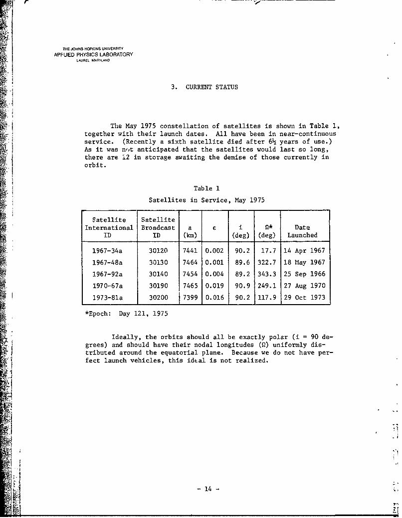
3. CURRENT STATUS

The May 1975 constellation of satellites is shown in Table 1,•} together with their launch dates. All have been in near-continuous

service. (Recently a sixth satellite died after 6½ years of use.)As it was n,,t anticipated that the satellites would last so long,

Sj there are 12 in storage awaiting the demise of those currently in

orbit.

Table 1

Satellites in Service, May 1975

SSatellite SatelliteInternational Broadcast a i Date

ID ID (km) (deg) (deg) Launched

1967-34a 30120 7441 0.002 90.2 17.7 14 Apr 1967

1967-48a 30130 7464 0.001 89.6 322.7 18 May 1967

1967-92a 30140 7454 0.004 89.2 343.3 25 Sep 1966

1970-67a 30190 7465 0.019 90.9 249.1 27 Aug 1970

1973-81a 30200 _7399 0.016 90.2 117.9 29 Oct 1973

S~*Epoch: Day 121, 1975

Ideally, the orbits should all be exactly polar (i = 90 de-grees) and should have their nodal longitudes (Q) uniformly dis-

• I tributed around the equatorial plane. Because we do not have per-fect launch vehicles, this ideal is not realized.

-14 -

A•t



I 4. OPPORTUNITIES FOR OBTAINING A FIX

Since the earth's rotation carries a user under an orbitlimb every 12 h and the satellite period (- 107 min) is short com-pared with a day, there are several opportunities for obtaining afix when a navigator is near the orbit plane. Typically, therewill be several fixes spaced approximately 107 min apart and thena long gap of 8 to 10 h. The sequence will then repeat. As this

•i •is true for any of the five satellites, fixes are availableroughly every 1½ h more frequently for a navigator near the polesand less frequently near the equator.

IO11

gI

gI° !

-15



5. ACCURACY AND QUALITY CONTROL

The operating agency, the Navy Astronautics Group, whoseheadquarters are located at Point Mugu, CA, is responsible formaintaining the satellite system on a continuing basis. Thisgroup of roughly 250 people maintains rigorous quality control

Nsi procedures over the accuracy of its computations and the perfor-• mance of the satellites, the oscillator drift, signal levels, the

ground station hardware, satellite and station clocks, etc. Somemeasure of their accomplishment in operating the system can beobtained from the following statistics (from Ref. 5):

" .From 11 October 1968 until 28 February 1975, therewere 22,871 memory reloads, 5 of which could not be

RMS verified as having properly refreshed the satellitememcry. For three of these five injections there is apossibility that the message being transmitted was goodbut its validity could not be absolutely determined.[Satellite reliability is defined as the percentage of

RZ in-service time the satellites were transmitting validnavigation information.] Between 11 October 1968 and18 February 1975 the NNSS satellite reliability was99.988%. Between 22 January 1973 and 28 February 1975,in-service reliability was 100%..

. Several other organizations independently certify the accu-racy (and integrity) of the system on a continuous basis. Forexample, at APL we have a navigation receiver that monitors allsatellites at every available opportunity. We have been doingthis since 1963. The data are used to navigate the site using theephemeris obtained from the satellite. Figure 2 shows typical re-sults.

The satellites are also routinely monitored by the TRANETSystem of tracking sites. (These tracking stations were originallyinstalled to support the development phase of Transit [1958-1963]

but currently play no role in its normal operation.) In addition,the Transit System data prov:de enough redundancy so that the sys-tem is, by and large, self-checking. For example, no data are ad-mitted to the orbit computation unless they are "consistent" withthe previously obtained orbit. Consistent means that a naviga-tion result produced with the data and the extrapolated ephemeris

Ref. 5. Navy Astronautics Group, Pt. Mugu, CA, private com-

munication, March 1975.

- 16 -

0 W EMT



100

45 passes"(all satellites)O long. = 29 m

0•O'lat. = 32 J•., ' 50 -D =264-277, 19744

.' 1

0-00

-50 0

I1 0 __ _ _ _ _ __ _ _ _j

0 50 100

Longitude (in)

Fig. 2 Transit Surveying Results.

lies within the expected neighborhood of the known station loca-g tion.

In addition to this criterion, the data must be reasonablyfree of gaps (data gaps are associated with instrumentation orSsignal-level problems) and satisfy internal consistency tests onthe noise. It suffices to say that the data editing is the mostintricate and involved part of the orbit determination computation(Ref. 6)..l aI

W Anyone with a Transit navigation receiver/computer can mea-* sure the internal consistency for himself simply by performing

repeated navigations at a fixed site.

4ff~

755

.1 Ref. 6. H. D. Black and B. J. Hook, "The Data EDITOR," APL/

JHU TG 756, 1966.

-i17 -

""A ihnteepctdnihoho fth nw tto oa


LAUREL MARYLAND

6. BROADCAST EPHEMERIDES

The ephemerides broadcast from the satellite are generatedby a least-squares fitting of the Doppler measurements to an ana-

¶i• lytical formulation of the Doppler shift (Ref. 7). The mathemati-cal modeling of the Doppler shift and the equations of motion ofthe satellite are as precise as we can write and currently includea (15 x 15) model of the geopotential, direct luni-solar perturba-tions, radiation pressure, polar motion, and the Jacchia model ofthe upper-atmosphere density (as part of the drag model) (Refs. 8,9, and 10).

For insertion in the satellite, the preci.sion ephemeris isfactored into a precessing-ellipse formulation p~lus corrections"to this approximate form. The combination of the two parts retainsall the precision of the original ephemeris. A word-length re-striction in the satellite memory forces us, as a final step, toround the ephemeris to the nearest 10 m. This numerical, randomnoise source is then ±5 m with a period of 2 or 4 min. This is aminor error source (see Table 6, Section 11) for a moving naviga-tor. The fixed navigator (surveyor) uses multiple passes fromseveral satellites and, as a consequence, many independent samplesof this noise; nevertheless, it is not a negligible error sourcefor users interested in the highest possible precision.

A larger navigation error source arises from incorrectlymodeled drag and radiation pressure acting on the satellite overthe extrapolation interval. Of these two, drag is the more seri-ous, in spite of the fact that drag is usually far smaller than isthe radiation pressure. This is because drag always opposes thealong-orbit motion; thus its effect is cumulative. Drag deter-mines how frequently the satellite orbit is redetermined. The nor-

•] mal mode of operation dictates that there be no measurable secular

(_ Ref. 7. H. D. Black, "Doppler Tracking of Near-earth Satel-lites," APL/JHU TG 1031, 1968.

Ref. 8. L. G. Jacchia, "Static Diffusion Models of theUpper Atmosphere with Empirical Temperature Profiles," SmithsonianContributions to Astrophysics, Vol. 8, No. 9, pp. 215-257, 1965.

Ref. 9. B. B. Holland, J. A. Yingling, and M. A. Walko,"The Second Generation Integration Routine (IGC)," APL/JHU TG 466(Rev.), 1970.

Ref. 10. A. Eisner, "Atmospheric Density Studies," APL/JHUTG 951, 1967.

-18-

STTHE JOHINS HOPKINS UNIVERSITY


o growth in the satellite position error over the extrapolation i.terval. The satellite position error is then dominated by geopo-tential modeling errors. Currently, near the minimum of the solarultraviolet cycle, this means that the satellite orbit must be re-determined daily.

•-I As we currently understand the Transit System, there is no

convincing reason for a user to compute ephemerides independentlyin hopes of achieving higher precision results. The error sourcesthat can be reduced by independent orbit determination (the drag-induced errors over the prediction interval,* the word-length-restriction error, the geopotential model errors) can also be re-duced simply by using a larger data population than would other-wise be necessary and all satellites. Moreover, the process canproceed in real time in the field. As each fix is obtained, themean of all fixes is updated. When this mean stabilizes with avariation less than (say) several meters, it is time to stop asmore data will not help. The March 1975 error budget and satelliteconstellation dictate that this will require 1 to 3 days and 20 to80 passes (see Fig. 2).

Ik The significant fact is that all orbit determination schemes-whatever the claims for their precision - are limited by the samethings, errors arising in

1. The instrumentation used to acquire the data;

2. The coordinates of the pole;

3. Ignoring the attitude motion of the satellite;

4. Higher order propagation (ionospheric) effects; and

5. The instability of the satellite oscillator.

All are on the order of a meter and, moreover, probably put long-term correlation (compared with the pass length) in the navigationerror. We will have more to say on these problems in a later sec-tion.

*The effects of drag (along-track bias) on the navigation resultchange sign for north- and south-going passes. Consequently thedrag error is largely cancelled.

~J & -19-

4..



7. SATELLITE CLOCK

By today's standards, the satellite clock need rot be very

accurate. This statement is true because system errors caused by

timing (bias) errors are never greater than IVSATI • At, IVSATI' 7000 m/s. If then the time bias lAti is less than 10-4 s, navi-gation errors caused by clock errors will be less than 1 m. Gen-erally the clock-associated errors are less than half this amount(Fig. 3). The clock is maintained as a routine part of the normalsystem operation by the Navy Astronautics Group. The techniqueused for "minding" (and utilizing) the clock is described inRef. 11. The primary time standard for Transit is UTC.

Periodically, at 6- to 12-month intervals, a portable cesiumclock (and frequency standard) visits all four tracking sites,after having been set at the Naval Observatory. Secondary cesiumstandards are maintained at all sites. Some recent results ofthese visits are shown in Table 2. We have omitted the Hawaii

10 0 I I I I I I I I I I I I I

80

60-40-

20- 600' 0

t41

V

Ref 1. .Mavn•Te prto o -te.aelie"l

4J 2EI* "%-20- T.".=p~t•

440o

15 55 95 135 175 215 255 295 335S~1973 (days)

• Fig. 3 Satellite 1967-92a Clock Error During 1973.

SRef. 11 C. Marvin, "The Operation of the Satellite Clock

•/• -•Control System," APL/JHU TG 523, 1963.

• •:•-• -20 -

r



Table 2

Time and Frequency Errors at theTransit Tracking Sites

77 rI Clock Error ,Frequency Bias i

Station Date (0s) (parts in 1012)

Maine Jan 72 164 Apr72 7 --

Oct 72 9 1

Apr 73 3 1SSep 74 15 2

V Minnesota Dec 71 10 4May 72 25 --

I Jun 73 17 7May 74 18 4

Nov 74 40 25

California Dec 71 1 --

May 72 11 3May73 1 --

May 74 1 3Nov 74 40 --

Station because it is operated in conjunction with a Naval Observa-tory time and frequency standard. The largest time bias measured

jI at the Hawaii Station is 5 vs.

The Naval Surface Weapons Center routinely evaluates the* satellite clock error using data obtained from the TRANET System,S5 i.e., a oystem of stations that are independent of the stations

used in setting the satellite clocks. Figure 3 shows their dataon Satellite 1967-92a for 1973. From the data, the satellite clockerror is generally less Lhan 50 vs. The system has maintained thisprecision since 1.968.

-V

- •.-• -• •% - 21 -

THE JOHNS HOPK(INS UNIVERSITY


4 8. GEOPOTENTIAL MODEL

There have been only four geopotential models used in theTransit System since the beginning. Listings of coefficients andgeoid maps (for the last two) can be found in Ref. 7. The develop-

¶ ment of these models was by and large the work of W. H. Guier,R. R. Newton, S. M. Yionoulis, and F. T. Heuring. We have com-piled Table 3 to illustrate the precision with which these modelswill determine a satellite orbit.

Table 3

Precision of Satellite Orbit

Orbit*Geopotential Precision

Model (m) Comments

APL 1.0 100-150 Zonals and sectorials through (4,4). Usedfrom December 1963 through December 1965.

2.0 Zonals and sectorials through (6,6). Usedfrom January 1965 through February 1966.

3.5 75-110 Zonals and sectorials through (8,8) plus afew resonant terms of order 13 and 14(Ref. 12). Used February 1966 throughJune 1968.

4.5 15-20 Complete through degree and order 11 plusmost terms through (15,15) (226 coeffi-cients). Used June 1968 through July1975. (Ref. 7)

WGS-72 5-10 Coefficient set complete through degreeand order 19, zonals through degree 24,and additional resonance terms throughorder 27 (479 coefficients). (Ref. 13)

*SaL:ellite altitude, 1100 km.

Ref. 12. W. H. Guier and R. R. Newton, "The Earth's GravityField as Deduced from the Doppler Tracking of Five Satellites,"J. Geophys. Res., Vol. 70, No. 18, pp. 4613-4626, 1965.

Ref. 13. T. 0. Seppelin, "The Department of Defense WorldGeodetic System 1972," The Canadian Surveyor, Vol. 28, No. 5,pp. 496-506, Ottawa, Canada, December 1974.

-22 -



As shown in Fig. 4, these model accuracies can be placed- in a common frame of reference using an analysis developed by

Holland et al. (Ref. 14), and Guier and Newton (Ref. 15).

100 ~1-80

60

T40 4

•, c"u 20C

-- 0

10

4

S2 I__ _ _I__ _ _II

8 10 12 14 16 18 20 22Degree n

Fig. 4 Satellite Position Error Caused by Truncating the Geopotential

Coefficients at Degree n, Satellite at 1 100-km Altitude.

Ref. 14. B. B. Holland et al., "Approaching Geodesy in the

1970's," AP7L/JHU TG 15,1969.

Ref. 15. W. H. Guier and R. R. Newton, "Status of the Geo-Ajdetic Analysis Program at the Applied Physics Laboratory," APL/JHUTG 652, 1965.

-23-

N.S



9. AT-SEA NAVIGATION

Ship navigation using Doppler measurements is, in principle,exactly the same as fixed navigation (surveying), but in practice,

• it is somewhat different. The reason is that the surveyor knowshis velocity with great precision; he is fixed relative to theearth. The at-sea navigator must have independent knowledge of hisvelocity. Moreover, he has a noise source that is not present inthe surveyor's computation: the erratic motion of his antennacaused by sea motion. (Since the doppler shift is a component ofrelative velocity, any unaccounted terms in the antenna motion arenoise/error sources.)

Several things can ameliorate these problems, but first we

should explain the net effect: Following Newton (Ref. 16), we de-rive that the principal effect of the navigator's velocity uncer-tainty is given by

S= r' - 2r cos (Q) + 1 16VI TD

S•cos-l(r cos 0-l.r2 sin () D

where

"r is the geocentric distance to the satellite in unitsof the earth radius,

S1 is tuie longitude difference between the navigatorand satellite when the satellite is at closest ap-proach,

1 6VI is the north component of the navigator's velocityuncertainty, and

TD is the pass duration.

The quantity in brackets lies between 0.5 and 1.1 for pass eleva-tions lying between 158 and 75*. Over this same elevation inter-val, it has a mean value of 0.65.

Ref. 16. R. R. Newton, "The U.S. Navy Doppler Geodetic Sys-tem and Its Observational Accuracy," Phil. Ttans. Roy. Soc. London,Vol. A262, pp. 50-66, 1967.

-24-


F APPLIED PHYSICS LABORATORYLAUREL,. MARYLAND

This equation is the basis of a handy rule of thumb thatis (almost) intuitively obvious:

'5 •K 16VI TD

For K I, this is just the dead-reckoning error at the end of thepass. For TD = 1000 s (typically), I6VI = 1 kt (0.5 m/s), and with

I. jK slightly less than unity, we get 350 m.

As a result (cf. Table 6), the error budget of the usualI, at-sea navigator is dominated by the velocity-uncertainty effect.This is, of course, not true for ships having high-quality inertialor Doppler sonar systems. A surprising fact is that an error in the

north-velocity component causes an error in the east-west position.For more elaborate discussions on this subject, see Newton (Ref. 16)K and Sluiter (Ref. 17).

The usual at-sea navigator could not care less if we provideenough precision in the fix for him to tell his bow from his stern."As a consequence, the 100- to 200-m error that comes from, say, a1/4- to 1/2-kt speed error is of little concern. On the other hand,there are some users for whom this is a serious deficiency, such asthe people using Transit in offshore oil exploration and oceanog-raphers using the system for at-sea magnetic anomaly surveys. Someof these users have elaborate ship-velocity instrumentation (Dopp-ler sonar combined with precision inertial equipment); some do not.

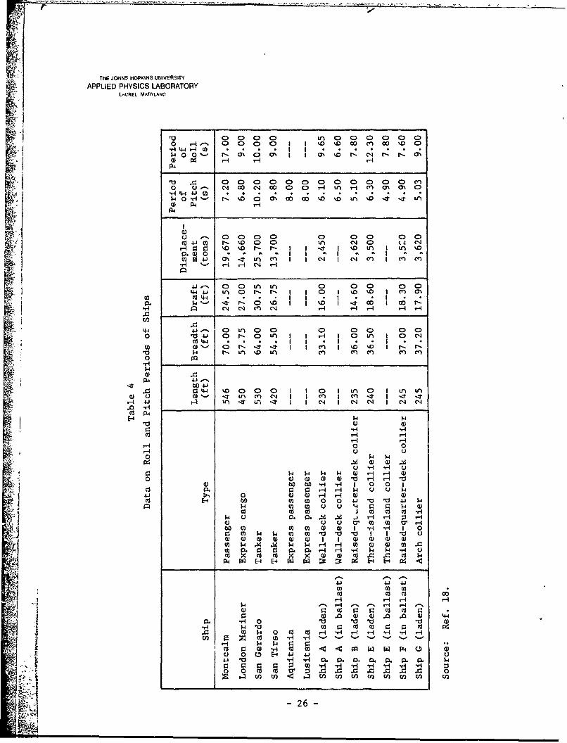
t The following remarks hopefully will help both types: Table 4,from Ref. 18, indicates that many, perhaps most, ships have naturalroll and pitch periods lying between 5 and 20 s. Manning comments

SI ... the natural period of pitching is usually between one-

third and two-thirds the natural period of roll.... Sinceocean waves are not usually of constant period for any sus-tained length of time, and since the longitudinal inertia of

- a ship is very great in comparison to its transverse inertia,it has been found that a ship pitches in its own naturalperiod a much greater part of the time than it rolls in itsown natural period. In other words, forced pitching occurs

* Ref. 17. P. C. Sluiter, "Relative Weighting of Satellite

Fixes," Proceedings of a Symposium on Marine Geodesy, New Orleans,LA, p. 151 et seq., 3-5 November 1969.

Ref. 18. G. C. Manning, "The Motion of Ships Among Waves,"Chapter 1, Principles of Naval Architecture, II, H. E. Rossell andL. B. Chapman, eds., Society of Naval Architects and Marine Engi-neers, p. 45, 1942.

- 25

z N ~ _

IA

THE JOHNS HOPKINS UNIVERSITY~

APIDPHYSICS LABORATORY

0 0 00011%0uiD 00000 .D0

-r-44 -l U) * . . I I~00 rý- M 0 m' %J g a' 90 P- C4 r-N.

0 in H m m 7

P.4

o M U-s %0 ) 0 0 " in 4 4 'a0-44

4 a) 0

0i H- H

4 4.1 0i 0 0- 0- 0 0 0 0 M(a 4-i 4 - . n c4 0~

C-(4 ('4 M~ 04 H H H

44O 0 0 00 0 00 ~ 41 0t 0' 0 in I CI H i 0 '

U)0 C';3 - -~- cnI I ' 0 I~. N34'- in) %.D ien ce cv M ' m cr

0 p

P.4 4jsC4.3

wJ- %0 0 00 I I0 If)n 0 I n in)0I 'T 0'-' cy) C 14 (I I cr) I n 17 - -T --T

H 4.3 t4 ~ v) 'T LI) CI C' (NJ 04N J C*-J

E-4 -

0 0

-H u0 ) 0 1 1 0 H HIr

Q) b 00-H H H

Hd0 - - 0 001> ) - - w - 140I 000 0 " H H0 v $

(0 Co Ofl H k4 00 r. I4p0 l 0. -y H H1.4 -) U- r -4 j

4.3 (a- 0 0 OH H O * 0

E-4- WO WX :2: 004.4 F4 Eq 04 .-

J 001 40 O

~~~Orj U)U ) 0 ) 0

0 0 0 0 I o It 0 0 0 0cc1- p~ 0~ CIS c 1-I H H U)ý 00 -H H

0- NE- E-4 4J~

4.1 -'i -. ' m-SP. m c. .

:j w H H Hr- H4 H9-H0 cd 0 :3 a 00

.1 0 1.4 0 .0 n 0 w ~

~ 0 U) H ''26''



that the period of pitching at sea is usually the ship's

natural period...."

Receivers for at-sea use should be chosen to avoid the 5-to 20-s period for the Doppler-counting interval, particularly ifthe necessary clinometer data are not provided to correct for theroll-pitch effects in the navigation computatlon.

It would be helpful if we could determine a ship's velocity

and position from a single pass of data. We have been unable tosatisfy ourselves that such a computation is practical. For a sat-ellite passing directly overhead (navigator in the orbit plane),the measured Doppler shift is very insensitive to the navigator'svelocity-east component. Were it not for the earth's rotation, wecould say it was "immune" to velocity-east. As a result, attemptsto determine both components of the navigator's position and ve-locity, using unaided Doppler data from a single satellite, do noti ' appear practical. For passes having elevation angles that exceed150, the longitude and velocity-north are strongly coupled and theeffects of velocity-east are practically negligible.

Q-2

I



10. PLANNED IMPROVEMENTS

Beginning in August 1975, a number of improvements areplanned for the Transit System. Some are designed specificallyto automate system operation and thereby cut the operation and main-

tenance costs. These will not be described here; however, reduc-tion in operating costs should have a beneficial effect on the sys-tem's life expectancy.

The changes of real interest to users are those that improvethe system precision (internal consistency); they are, first, in theorbit-determining software and, second, in the hardware.

10.i Orbit-determination Software Changes

We are:

1. Replacing the APL 4.5 geopotential model with the WGS-72model;

2. Consistent with item 1, updating the GM (gravitational

constant times the earth mass) from its currently usedvalue of 398601.5 ± 0.6 km3 /s 2 (Ref. 19) to the moreIi recent determination - including the atmosphere - of

398600.8 ± 0., km3 /s 2 (Ref. 20). We are leaving thespeed of light unchanged at 299,792.5 km/s;

3. Altering the coordinates of the four tracking sites tobring greater internal consistency to the overall net-work. These changes are given in Table 5;

Ref. 19. W. L. Sjogren, "The Ranger III Flight Path and ItsDetermination from Tracking Data," JPL Technical Report, 32563, 22,Jet Propulsion Laboratory, Pasadena, CA, 15 September 1965.

Ref. 20. P. B. Esposito and S. K. Wong, "Geocentric Gravita-tional Constant Determined from Mariner 9 Radio Tracking Data,"Jet Propulsion Laboratory, Pasadena, CA, 1972. (Paper presented atthe International Symposium on Earth Gravity Models and RelatedProblems, St. Louis, MO, 16-18 August 1972.)

-28-

R'i.



2 4 -•Table 5

V •Changes to the Transit Stations' Co r1inates(in meters)

'1 Station Location Latitude Longitude Fadius

1 Maine (311) -0.3 -4.6 +0.6

Minnesota (321) +2.0 +3.2 +5.4

California (330) +1.8 0.0 +0.3

I Hawaii (340) +6.1 +0.6 -4.5

Mean Change +2.4 -0.2 +0.5

Note: To be implemented in the fall of 1975.

T 4. Implementing the (main) body-tide perturbation on thesatellite. This force had previously been neglected; and

5. Introducing an improved model of the radiation pressureforces.

I The changes are scheduled for implementation beginning in

August 1975. No changes are required of any user. We do suggestthat the numerical integrity (consistency) of the older navigation

I programs should be reexamined to ascertain that they do not intro-duce spurious numerical noise as large as 1/2 m. We are leavingthe angular velocity of the earth unchanged at 7.29211585 x 10-5

rad/mean-solar-s because there is nothing to be gained by changingit.

10.2 Hardware Changes

A new type satellite is being introduced into the constella-tion in late 1975. Of principal interest is the DISCOS* device(Ref. 21) and a high precision clock. These improvements will be

i I discussed in detail.

*Disturbance Compensation System, a device that accelerates or de-celerates the satellite to compensate for the effects of drag andradiation pressure.

Ref. 21. Staff of the Space Department, The Johns HopkinsUniversity Appl .ed Physics Laboratory, and the Staff of the Guid-

Q ance and Control Laboratory, Stanford University, "A SatelliteFreed of All But Gravitational Forces: TRIAD I," J. Spacecraftand Rockets, Vol. 11, No. 9, pp. 637-644, 1974.

- 29-

r

-THE JOHNS HOPKINS UNIVERSITY

APPLIED PHYSICS LABORATORYLAURCL. MARYLAND

11. WGS-72 GEOPOTENTIAL MODEL

The single-pass error budget for a surveyor is given inTable 6 both "before" and "after" the introduction of WGS-72.1

Table 6

Li Transit System - Surveyor's Single-Pass Error Budget

Meters

1. Uncorrected propagation effects 1-5(3rd order ionospheric and ne-glected tropospheric effects)

"2. Instrumentation (navigator 1-6satellite oscillator phase (See note)jitter)

3. Geodesy (uncertainty in the 15-20 5-10geopotential model) (APL 4.5 . (WGS-72)

4. Incorrectly modeled surface 10-25forces (secular error growthdue to incorrect period, dragand radiation pressure)

5. Unmodeled UTl-UTC effects andincorrect coordinates of the pole

6. Ephemeris rounding error (last 5digit of ephemeris is rounded)

rss 19-33 12-28(APL 4.5) (WGS-72)

Note: We have some data that indicate that the Geoceiver oscillator/Transiti satellite oscillator contribution is appreciably less than 1 m (Ref.

22). This performance is not unique to Geoceiver but characteristicof the more modern receivers. For the older SRN-9, the contributionis 3 to 6 m (Ref. 7).

4

Ref. 22. B. B. Holland, "Uses of Geoceiver as a Geodetic In-strument," Proceedings of COSPAR XIII, Madrid, Spain, 10-24 May1972, Akademie-Verlag, Berlin, p. 71, 1973.

-30-

0ý- W- "ýý; ~ ~ ~ ~ ~ ý fT __4z -___, -%_- - .W .--- ,:--- *



It is clear that implementing WGS-72 will not have a strik-ing effect on the single-pass error budget; Eor the existing con-stellation, the budget will continue to be dowinated by items 3

and 4 from Table 6. We decided to implement WGS-72 for the follow-

ing reasons:

1. There is a beneficial side effect even for existingsatellites. Reducing the correlated (geodesy) errors

1• gives improved access to the orbit state vector, andtherefore the orbit extrapolation errors are diminished.(Since it is not clear how this improvement will beutilized, we have not reflected this improvement In theerror budget.)

1 2. We found that if we restructured the computation of theU- force terms in the satellite equations of motion, we

could implement WGS-72 with a minimal increase in com-S I puting time.

3. The integrity of any previously derived Transit re-sults would be preserved; the discontinuity in results

K (Table 5) when the system is changed from one geopoten-tial model to another would lie within the previouslyadvertised 1- to 5-m precision (Ref. 23) over most of

3 the western hemisphere. In the Indian Ocean the differ-ences reach a peak of 15 m. We were careful to preservethe longitude reference of the coordinate system whichis implicit in the station coordinates (Ref. 24).I

4. Of some real significance for the new satellite is that,with the single-axis DISCOS system, there is good reason

Sto believe that drag errors will be reduced by a factor* of 10 (see Section 16). If this turns out to be true,

then the largest error sourses for fixed site navigation-t| will be appreciably reduced. For the DISCOS-equipped

satellite, the single-pass error budget will become 7 to13 m; with the combination of DISCOS and WGS-72, we willhave halved the current 19- to 33-m error budget.

Ref. 23. V. L. Pisacane, B. B. Holland, and H. D. Black,"Recent (1973) Improvements in the Navy Navigation Satellite Sys-tem," Navigation, Journal of the Institute of Navigation, Vol. 20,pp. 224-229, 1973.

I Ref. 24. G. Gebel and B. Matthews, "Navigation at the PrimeMeridian," Navigation, Vol. 8, pp. 141-146, 1971. (Note: A re-cent redetermination of the connection between the astronomicalmeridian and the geodetic meridian replaces the 5.64" [given inthis paper] with 5.69" ± 0.17".)

*1t - 31-

THE JOHNS hOPKINS UNIVERSITY

APPLIED PHYSICS LABORATORYLAUP.L MARYLAND

There is another reason, a very human reason, for implement-ing WGS-72: Describing coordinate systems, geopotential models,datums, etc., is a very tedious job. It is a great convenience tosimply say, "the Transit System is on WGS-XX."

11.1 Comparison with Other Geopotential Models

Since certain aspects of WGS-72 are classified, we are notfree to describe it in great detail. This fact does not impugn itsusefulness in deriving positional information. We have performed anumber of experiments comparing orbits derived with WGS-72 withthose obtained using other geopotential models, and leaving allother parts of the process(ors) unchanged.

The orbit error is most conveniently represented as stationposition error (at known sites) resolved in orbit-related coordi-nates (Ref. 7).

We determined a single-state vector (utilizing all data col-

lected at the four tracking sites over two 4-day periods) employingWGS-72. After the orbit determination computation was complete,we then treated each pass of data independently in a station naviga-tion computation. The navigation "errors" become, then, a measureof the internal consistency of the entire system, the earth modelincluded. We repeated the determination for

1. GEM-I (Goddard Earth Model 1) (Ref. 25),

2. GEM-6 (Ref. 26),

3. SAO Standard Earth 3 (Ref. 27), and

4. APL Mk 4.5.

The results are summarized in Table 7 where we show the rms errors4 for both position components. The rms is taken over all data in

the 4-day span.

Ref. 25. D. E. Smith, F. J. Lerch, and C. A. Wagner, "Gravi-tations Field Model for the Earth," Proceedings of COSPAR XIII,Madrid, Spain, 10-24 May 1972, Akademie-Verlag, Berlin, 1973.

Ref. 26. F. J. Lerch, J. E. Brownd, J. A. Richardson, andJ. S. Reece, "Gravitational Models GEM-5 and GEM-6, 1974," contribu-tion to The National Geodetic Satellite Program Final Report, Ameri-can Geophysical Union, Washington, DC, to be published August 1975.

Ref. 27. E. M. Gaposchkin, ed., Smithsonian Standard Earth

III, Smithsonian Astrophysical Observatory Special Report 353, 1973.

- 2-


-~ __ *LAUREL MARYLAND

"I Q) -4 0 040

c, _ _ _ _ _00_ _ _ _ _

01

-H 0 0ý c

0 w

bo 0 IT a

-H

o0w

V.$- 0o 0'0co~ r.p '

% O 0n 4 N '. L%

co HH 0

m~ a) 1 4-Ia) I 41- 4J () 4

4~a) ~ ca :3

ca *dH H 00~zwr $4I

1'Q 0) 4to-). 0 co 0'.0

r: -

cq 0 H . 0 H 4)

1 :3 tO " $4

-N 77 -1 C

0'.a 0'0 '

It ca wI a)) cII... C1 (a m U

cIrCl Cco Cl) Nc U) Nn I'

1 04 0. 0. r9 ~~.t 0 --- 0 -~H *t In ' intnI In If)

ail-i


APPLIED PHYSICS LABORATORYLAUREL MAPYLANO

From the data it would not be difficult to choose WGS-72 inpreference to the others. An impressive fact is that GEM-I was de-termined from optical data, whereas WGS-72 (and APL 4.5) were de-termined using a large population of Doppler data, in particulardata from the Transit satellites.

As a part of these tests, it was necessary to extrapolatethe ephemeris 96 h into the future and repeat the navigations. Un-certainty in drag and radiat.•n pressure corrupt the orbit accuracy,but by the same amount for all model cases; the more accurate perioddetermination possible with WGS-72 is clearly apparent. Graphsshowing the along-orbit error component are shown in Figs. 5 through8 for GEM-I, GEM-6, APL 4.5, and SE 3 geodesy, respectively, with

4 the corresponding WGS-72 results for easy comparison. The left halfof each figure shows the orbit error during the data span. Theright half shows the error during the 4-day prediction. (Operation-ally, the satellite-borne ephemeris is replaced before the seculargrowth rises above the geopotential errors.)

We will have more to say about this secular error in Sec-tion 15.

As another check on the internal consistency of the system,we repeated EXP 1 of Table 7 using data from three, rather thanfour, of the available stations. The data from the fourth station(Minnesota) were used to measure the precision of the resultingephemeris. During the 4-day period, 24 passes from the fourthstation were used in a navigation solution. The mean of the 24fixes differed 0.6 m in latitude and 1.2 m in longitude from ourbest estimate of the true station position.

S J

~i'

334

M-34-

THE JOHNS HOPKiNS .JNIVERSITY


0 0

9) 0

a. (D9

*. (o Mo99* oC

D in cu min a- aD (n

* l . 04.*L 0

*0 9 L.O

0* 9 000 0)* ~0*

0 0 9 0) 0 :I.. L. oLr oLf oL

4& *w slaod o aw. siuaua. wEoj I..oBul .oij I~q* * E

93

r


APPLIED PHYSICS LABORATORYL.AUR1EL MARYLAND

40 aC- 4

9 9do

C1 0 0

r* c U.

* aI

0 C

.0 0

(D2 4- < (o 1 oQ) c* III c

CL 0 LCL

** T co N c: 10 20u - - u 0l o -

* .

0~0

co F0 00

N (U cTU N

(wJ slaodo (wJ siuaodwojo-j 1!(NJu l 0oj ~j-u l

36.


APPLIED PHYSICS LABORArORYLAUREL MARYLAND

12. GEOID HEIGHT CONTOUR MAP

We are frequently asked what geoid map to use with theTransit System. The correct (May 1975) map is sl •wn in Fig. 9;it is rigorously consistent with the currently used (APL 4.5) geo-potential. This .odel is consistent with an ellipsoid having asemi-major axis of

• I "Ia--6378.137 km

and a flattening of

f = 1/298.25.

It is common to report geoid heights relative to various ellipsoids.*W It is not vitally important which ellipsoid is used so long as

Lhe map and associated ellipsoid parameters are used in a consistentI fashion to construct the distance from the coordinate center (earth5 mass-center) to the navigator's antenna. It is this distance which

is important, rather than any of the mathermatical pieces used in

constructing it.

There is a 7- to 9-m inconsistency in most navigators' pro-grams, as we originally recommended values of

S I a = 6378.144 km and

g f = 1/298.23.

Before we describe how to repair this inconsistency it should bepointed out that, as of late 1975, the correct (WGS-72-consistent)

E" value will be

a = 6378.135 km and

f = 1/298.26.

*• These values are close enough to the APL-4.5-consistent values that3 •we can correct immediately to the WGS-72 values.

The simplest way to compensate for the inconsistency men-tioned above is to alter the antenna height (height above mean sea

Slevel). The recipe is as follows:

- W *Although the geoid height can be computed without directly utiliz-

ing the ellipsoid parameters (Bruns' formula), the parameters are1 ýusually lurking in the background and therefore implicitly in-

volved.

-37-

THIF JOHNS HOPKINS UNIVERSI Iy

APPLIED PHYSICS LABORATEORyLAUREL M.RYLAND

0

C) c"IC) C)

-Y 0(0

Cv)

0 00

W_ 0ccv)

0co

C-

0

co o

U) 0 b-1 CD cv)cv

~4 I -

""J-38-

THE JOHNS HOPKINS UNIVERSfTY

APPLIED PHYSICS LABORATORYS ! LAUREL MARYLAND

8-7-

I _

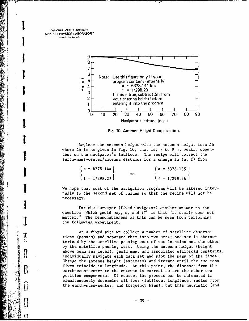
6 Note: Use this figure only if yourE 5 - program contains (internally)

S4- a = 6378.144 kmI f = 1/298.23S3 - If this is true, subtract Ah from

2 - your antenna height before"" 1 - entering it into the program

0 10 20 30 40 50 60 70 80 90

Navigator's latitude (deg

Fig. 10 Antenna Height Compensation.

Replace the antenna height with the antenna height less Ah

where Ah is as given in Fig. 10, that is, 7 to 9 m, weakly depen-dent on the navigator's latitude. The recipe will correct the

earth-mass-center/antenna distance for a change in (a, f) from

t~ =a 6378.144 t a = 6378.135

f = 1/298.231 f = 1/298.26

SWe hope that most of the navigation programs will be altered inter-nally to the second set of values so that the recipe will not benecessary.

For the surveyor (fixed navigator) another answer to thequestion "Which geoid map, a, and f?" is that "It really does not

I matter." The reasonableness of this can be seen from performingthe following experiment.

"At a fixed site we collect a number of satellite observa-"tions (passes) and separate them into two sets; one set is charac-2 •• terized by the satellite passing east of the location and the otherby the satellite passing west. Using the antenna height (heightabove mean sea level), geoid map, and associated ellipsoid constants,

4 individually navigate each data set and plot the mean of the fixes.: Change the antenna height (estimate) and iterate until the two mean"fixes coincide in longitude. At this point, the distance from the

%A earth-mass-center to the antenna is correct as are the other two

position components. Of course, the process can be automated toA • ' , simultaneously determine all four (latitude, longitude, radius from

the earth-mass-center, and frequency bias), but this heuristic (and

~ I,] -9

_Z 4"



practical) technique is usefuJ in understanding why the systemdoes not really require a specific geoid map: The distance fromthe mass center is determinate if multiple passes are used. Re-sults of such an experiment are shown in Fig. 11.

After the fall of 1975, the at-sea navigator can continueto use the geoid map shown in Fig. 9. An examination of a numberof geoid maps (Refs. 26, 28, 29, 30, and 31) and a comparison ofthem with Fig. 9 have convinced the writers that there is littlereason to replace it.

7it

pp. 5377-5411, 1974.

Ref. 29. R. H. Rapp, Numerical Results from the Combinationof Gravimetri,:z and Satellite Data Using the Principles of LeastSquares Collocation, Ohio State University Report No. 200, March1973.

Ref. 30. R. H. Rapp, Procedures and Results Related to theDirect Determination of Gravity Anomalies from Satellite and Ter-restrial Gravity Data, Ohio State University Report No. 211, July1974.

Ref. 31. S. M. Yionoulis, F. T. Heuring, and W. H. Guier,"A Geopotential Model (APL 5.0-1967) Determined from SatelliteDoppler Data at Seven Inclinations," J. Geophys. Res., Vol. 77,No. 20, pp. 3671-3677, 1972.

-40-



Station navigations using various station radii

East

AT - tr 20m A ý &

AA

Z I

East West

r = "correct" -

-140-120-100 -80 -60 -40- 0 20 40 60 80 100 120* 6Xlm)

Ar =-20m

.:• •..East

rlsdlWestN "!•Circles indicate la• " U •Pass west of station

•! , • APass east of station

1 .Fig. 11 Determination of the 3-Dimensional Position (all satellites, days 40-43, 1974).

2J , -41-

74 ,-- FOM-5



13. SUN- AND MOON-INDUCED EARTH BODY-TIDES

To compute the effects of the body-tides (the main semi-diurnal tide) on a near-earth satellite, the geopotential of theearth is augmented by*

iIVT -k rd- \MJ rd! Ir P2 (rt. r)(1

and the resulting acceleration of the satellite is

-(V vT) .

In this equation

k is the tidal Love number, 0.336 (Ref. 34), 0.309(Ref. 35);

R0 is the radius of the earth;

GM is the product of the gravitational constant andthe earth mass (398600.8 km3 /s2 ± 0.4) (Ref. 20);

M /M is the tidal-raising mass/earth mass;t e

*From Refs. 32 and 33.

Ref. 32. R. R. Newton, "An Observation of the Satellite Per-turbation Produced by the Solar Tide," J. Geophys. Res., Vol. 70,pp. 5983-5989, 1965.

Ref. 33. R. R. Newton, "Tidal Numbers and Phases as Deducedfrom Satellite Orbits," APL/JHU TG 905, 1967.

Ref. 34. R. R. Newton, "A Satellite Determivation of Tidal"Parameters and Earth Deceleration," Geophys. J. Roy. Astron. Soc.,Vol. 14, pp. 505-539, 1968.

Ref. 35. K. Lambeck, A. Cazenave, and G. Balmino, "SolidSEarth and Ocean Tides Estimates from Satellite Orbit Analysis,"Rev. Geophys. Space Phys., Vol. 12, No. 3, pp. 421-434, 1974.

J -42 -

STHE JOHNS HOPKINS UNIVERSITY


r is the vector from the earth mass-center to thej° satellite, the point where the potential is to beevaluated, r is the corresponding unit vector,and r, the length of r;

I rd is the distance to the tide-raising body; and

-I rt is the unit vector through the tidal axis, i.e.,

cos cos(a + at)r A cos (6) sin (a + a

' I sin 6

S* wherein a, 6 are the instantaneous coordinatesI (right ascension and declination) of the tide-

raising body and ao is a small angle, "the tidalphase lag" (0.023 -ad for the sun, 0.026 for the3 moon). Lambeck (Ref. 35) gives 0.0087 for both;

P and

) is the 2nd order Legendre polynomial2 [3 cos2 -]poyoil=2

A term like Eq. (1) must be included for both the sun and the moon.J The amplitude of the sun body-tide is about half that of the moon.Because of the higher frequency associated with the lunar effect,about 13 times the frequency of the solar one, the net effect ofI the moon on the satellite is about 1/6 that of the sun (Ref. 36).

The determination of the Love numbers (and their associated!I phaces) is currently an active area of research (Refs. 35 and 37).5 A current goal is to reducb the satellite-determined values for

the effects of the ocean tides. Lambeck estimates this effect tobe 4 to 9%. Our concern is different; consequently we are usingNewton's values which were determined from the Transit satellitesand were not corrected for the effect of the (ocean) tides. Thisis internally consistent with our usage.

FRef. 36. R. R. Newton, "Applied Ancient Astronomy," APL

Technical Digest, Vol. 12, No. 1, pp. 11-20, 1973.

Ref. 37- B. C. Douglas, S. M. Klosko, J. G. Marsh, and R. C.. Williamson, "Tidal Perturbations on the Orbits of GEOS-I and GEOS-2,"

NASA Report X553-72-475, 1972.

-43-

'91 THE JOHNS HOPKINS UNIVERSITYi •APPLIED PHYSICS LABORATORYSLAUREL MARYLAND

The principal effect of the body-tide perturbation is an• 1 oscillation in the "along-track" (along-orbit) direction that has

a period which is one-half the orbital period of the tide-raisingbody (14.5 days for the moon, 6 months for the sun). * To illus-trate this effect and to check once again the numerical consis-tency of our program, we performed the following experiment.

Using the same set of initial conditions (a = 1.17,e = 0.0021, i = 89.68, Q = 3390, d = 40, 1974), we computed theposition of a satellite with and without the moon body-tide. Wethen differenced the ephemerides at common times and resolved thevector difference in the along-track direction. Results of this

' simulation, produced for an 8-day ephemeris, are shown in Fig. 12.This curve is the sum of a linear-time function and a 14.5-day

I sinusoid. The linear term arises because the two orbits do notoccupy the same potential surface and consequently have slightly

. different periods. The sinusoid arises because of the periodicpotential field associated with the lunar tide.

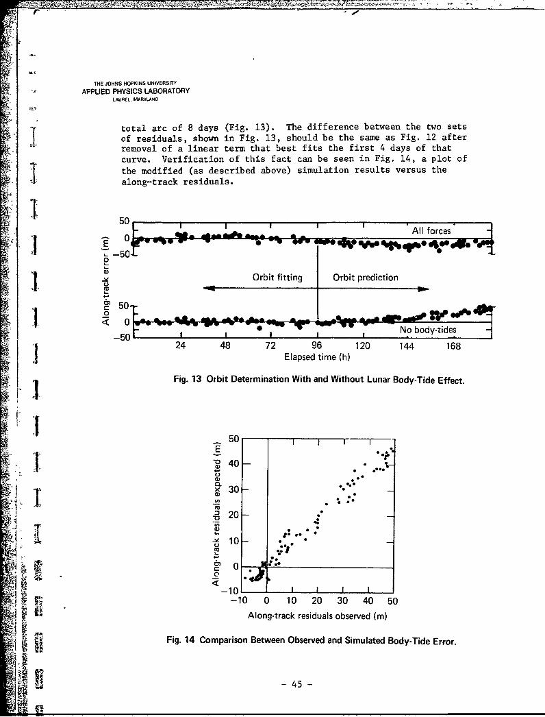
Now, to demonstrate the effect of the moon body-tide onnavigation we selected a 4-day data span and determined two orbitsthat fit the data, one with all forces included, one without body-

tides. While these orbits agree well with the data (and with eachother) over 4 days, they do not agree well when extrapolated to a

2•10 I I I I I I11 1 1 I 1"'

10)8 8o-

.4- 60

40

20

< 0 12 24 36 48 60 72 84 96 108 120 132 144 192

Time (h)

Fig. 12 Expected Along-Track Residuals (lunar body-tide effect).

*If the orbit is redetermined at frequent intervals - frequent mean-1 ing closely spaced compared with the lunar period - the tides have

almost ao effect on the navigation result; no effect even if theyare ignored.

1 - 44-

ol~



total arc of 8 days (Fig. 13). The difference between the two setsof residuals, shown in Fig. 13, should be the same as Fig. 12 afterremoval of a linear term that best fits the first 4 days of thatcurve. Verification of this fact can be seen in Fig. 14, a plot ofthe modified (as described above) simulation results versus thealong-track residuals.

50 •_I 1 1 " All forces 4] •t~ -a--.-- -- ._ ,..-50

0)a)Orbit fitting Orbit prediction

4O

I ~~50--~] ,-a- .. .. AAdl-&e-50 W S PWNo body-tides

24 48 72 96 120 144 168Elapsed time (h)

Fig. 13 Orbit Determination With and Without Lunar Body-Tide Effect.

50

"0 40--

• ~x 30 -0*0

2 -

0

10

"-10- "

0" -10 0 10 20 30 40 50

SAlong-track residuals observed (m)

Fig. 14 Comparison Between Observed and Simulated Body-Tide Error.

-45-



14. RADIATION PRESSURE

Radiation pressure is a very tricky force to deal with inthe numerical integration algorithm used to construct the satel-lite ephemeris. It is tricky because the force has a discontinuitywhen the satellite passes into, or out of, the shadow of the earth.This on-off time can occur anywhere with respect to the beginningof the (discrete) integration step. Since forces are evaluatedonly on the discrete steps, numerical integration errors arise asa consequence. An analysis of the effect (Ref. 38) shows that (onthe average) the orbit error grows as the 3/2's power of (orbit)arc length and at the end of 14 satellite revolutions (s 1 day) itis aboue 2 m (the radiation pressure is about 1 dyale/m 2 ). To re-move this error source, several necessary pieces were assembled.

1. The integration algorithm was shown to give the right"answer for a discontinuous force when the discontinuitywas replaced'with a piece-wise linear function,

I ON

x OFF

providing the length of the ramp was equal to the numeri-cal integration step-size. The obvious was then imple-mented.

2. With an analytical formulation of the orbit, we keep arunning prediction of the shadow-crossing geometry.

3. We center a ramp on the transition point with the lengthof the ramp equal to the integration step-size.

This sounds quite simple but making the program smart enough tocope with the satellite just grazing the terminator complicates thematter!

W

Ref. 38. W. L. Ebert, "Errors in the Ephemerides of Satel-lites Caused by Numerical Integration," APL/JHU TG 1233, 1973.

1 - 46-


APPLIED PHYSICS LABORATORYLAVREIL MARYLAND

We also designed and programmed a version to include the

S j penumbra/umbra transition and the albedo. These elaborations donot currently affect the derived orbit in any significant way:the orbit frequency term, generated by the albedo, is currently an

order of magnitude less than the corresponding term in the geopo-tential uncertainty.

R !

44i

ni

• l

I

Lj

5-47

-

t



15. DRAG COMPENSATION (DISCOS)

As a result of the Transit improvement program, the newtype of satellite to be added to the system has vastly improvedhardware (Ref. 39). The satellite is called TIP-II (Fig. 15).One of the new features is DISCOS, which removes the along-trackcomponent of drag and radiation forces.

In the DISCOS, a closed loop thrusting system keeps thesatellite centered on a "proof mass" that is shielded from thesatellite surface forces. As a result, the satellite is con-strained to the proof-mass orbit which experiences no drag. Anexperimental 3-axis system was successfully flown in the TRIAD-Isatellite in 1972 (Ref. 21). To simplify the system, the opera-tional version was reduced to a single (along-track) axis compen-sation. The single-axis system requires precise, 3-axis stabiliza-tion. The thrust is supplied by ionized Teflon thrusters.

The presence of DISCOS improves the accuracy (predictabil-ity) of the satellite ephemeris. With the drag removed, theephemeris precision becomes limited by the geopotential modelerrors. As indicated earlier (Table 6, item 3), this precisionwill be under 10 m with the WGS-72 geopotential model.

TRIAD-I orbit experiments (Ref. 40) showed that the ephem-eris could be extrapolated with the DISCOS for at least a weekwithout appreciable degradation in accuracy. This reduces systemoperation costs by requiring less frequent orbit computation.

Ref. 39. J. Dassoulas, "The TRIAD Spacecraft," APL Techni-cal Digest, Vol. 12, No. 2, pp. 2-13, 1973.

Ref. 40. R. E. Jenkins, "Performance in Orbit of the TRIAD4 DISCOS System," APL Technical Digest, Vol. 12, No. 2, pp. 27-35, 1973.

-48-

THE JOHNS HOPK(INS UNIVERSITY

'V APPLIED PHYSICS LABORATORYLAUREL HAPYLAND

V

Fig. 15 TIP Satellite, Artist's Concept.

-49-



16. FLIGHT COMPUTER AND EXTRA MESSAGE

Decreasing the orbit error below 10 m will not immediatelybenefit the iavigator using the broadcast ephemeris. This is truebecause of the rounding errors (among other reasons), discussed inSection 6. However, there is another hardware feature of the newTransit satellite that provides the necessary flexibility to removethis error source. Included in TIP is a general-purpose computerto replace the hardwired memory and an additional ephemeris modu-lation that does not affect present receivers.

The flight computer is a 32k, 16-bit-word general processorwith a 4.8-Us memory access time. The computer is about the ilk ofthe second-generation computers such as the IBM 7094. The softwaresystem currently implemented in the flight computer manages theloading and rebroadcasting of the ephemeris and also controls thesatellite clock. Ten days irth of ephemeris can be stored, andthe broadcast ephemeris is m-de to look exactly like the presentmessage. The computer is programmable from the ground.

The important point is that the flight computer permits usto change the message content by reprogramming the management soft-ware. (Whatever we do, no mandatory changes will be required ofany user.)

The extra ephemeris modulation is a phase modulation that is"transparent to existing receivers." It is superimposed on thenormal "double-doublet" ephemeris modulation (Ref. 41). The newmodulation has a data rate that is one-half the current 50 bps.The content of the message will be controlled by the flight computer.

174

Ref. 41. R. J. Heins and E. F. Prozeller, "Development of aCompact Ephemeris Recovery System for the AN/SRN-9/PRN Receiver,"j ;• APL/JHU Quarterly Report C-SQR/74-3, July-September 1974.

-50-

r


APPLIED PHYSICS LABORATORY

I LAUREL MARYLAND

17. CLOCK IMPROVEMENTS

i

The new TIP satellite contains hardware that greatly im-proves the potential precision of the real-time satellite clock.The IPS (incrementally programmable synthesizer) allows precise

V control over the satellite oscillator output. The IPS sysLemoperates as a "programmable black box" and modifies the 5-MHzoscillator frequency according to the transfer function:

Icout Cosc B

A and B are control parameters that can be commanded from the3 ground into the IPS through the flight computer. A and B areI. Ton the order of i0u. A exerts fine control while B is the coarse

control. A portion of the real-time software system in the flighti computer is devoted to manipulating A and B to correct for oscil-

lator offset, aging, drift, and random jumps.

The system can be used to maintain a high-precision clock3by observing the satellite time on the ground and injecting IPS

control parameters for clock steerage. The closed loop system isshown in Fig. 16. The IPS filter-and-control program is a Kalmanfilter that recursively processes the clock error measurementsI and computes the controls (A, B, f) required to steer the clockerror to zero over the specified time interval T. The control

i parameters are then injected into the flight computer from a3- ground station.

The time constant of the loop is quite long (compared with3 most control loops) since the measurement and injection rates are3, set by the times when the satellite is visible. An injection rate

W 1of about one a day is the practical lower limit with the currentground system. Generally, the more often the controls can be ap-plied, the more accurately the clock can be held to the groundreference. The one-a-day rate was chosen to accommodate the satel-lite visibility schedule of the operational ground system.

The oscillator model used in the IPS Kalman filter program

is one of a drifting oscillator that undergoes random (white) jumpsin drift-rate and random jumps in frequency on the average of onceper day. Ground tests of the system using a prototype oscillatorworked well with a one-a-day injection cycle when the standard de-viation of the random jumps in the filter noise model was set at

- 51-

•5i

r oo



00

00

E44

-52- C

I THE JCHNS HOPKINS UNIVERSITY

APPLIED PHYSICS LABORATORYLAM.REL MAAfLANO

1012 in frequency and 2 x 10-2 per day in drift. We were able tocontinuously control the clock error to i0- 7 s for about I week,*which is testimony to the stability of the oscillator. The ulti-mate clock accuracy in orbit depends, of course, on the Prystalperformance, particularly the absence of large random jumps. TheIPS and the time-measurement filter program merely allow correc-tion for the observed long-term (longer than a day) random be-havior of the oscillator.

I All preliminary tests indicate the flight oscillators inthe new satellite should perform as well as the prototype. Ifaccurate ground measurements can be made of the clock epocherrors, then the potential exists for 100-ns control.

Another new subsystem provides the capability for satelliteI clock epoch to be received on the ground with nanosecond precision.

This is the pseudorandom noise (PRN) phase modulation that is im-

posed on the satellite 150- and 400-MHz carriers. This modulation,which is transparent to present navigation receivers, provides aranging system as well as a time recovery system to any receiverequipped to recover PRN. The two-frequency PRN data can be cor-rected for first-order ionosphere time delays and the propagationtime delay can be determined from the "navigated" slant range.

NOTE

I The TIP-II satellite was launched on 12 October 1975. The

solar (power-generation) panels failed to deploy. A second of theseries is scheduled for launch in mid-1976.

I

I

*We actually ran the test for over a month, but a week was thelongest continuous span we could get without a thunderstorm caus-ing a power loss.

-53-

W5

h THE JOHNS HOPKINS UNIVERSITYAPPLIED PHYSICS LABORATORY

LAUkEL MARYLAND

ACKNOWLEDGMENT

The writers are indebted to their colleagues in the SpaceAnalysis and Computation Group, in particular, to Messrs. StanleyDillon and Bruce Holland and Dr. Ward Ebert for their assistancewith the computer experiments. Appreciation for supplying statis-tics on Transit System operation is due the personnel at the NavyAstronautics Group, Point Mugu, CA.

This work was supported by the United States Department ofthe Navy, Strategic Systems Projects, under Contract N00017-62-C-0604. We acknowledge this support with thanks.

Li

g, - 54-


LAUREL MARYLAND

IREFERENCES

1. F. T. McClure, Method of Navigation, U.S. Patent No.3,172,108, filed 12 May 1958, issued 2 March 1965.

2. W. H. Guier and G. C. Weiffenbach, "Theoretical Analysisof Doppler Radio Signals from Earth Satellites," APL/JHUBB-276, 1958.

3. W. H. Guier and G. C. Weiffenbach, "A Satellite DopplerNavigation System," Proc. IRE, Vol. 48, pp. 407-516, 1960.

4. R. B. Kershner and R. R. Newton, "The TRANSIT System,"J. Inst. Nay., Vol. 15, pp. 129-144 (see p. 140), 1962.

5 9. Navy Astronautics Group, Pt. Mugu, CA, private communica-tion, March 1975.

6. 11. D. Black and B. J. Hook, "The Data EDITOR," APL/JHUTG 756, 1966.

I 7, H. D. Black, "Doppler Tracking of Near-earth Satellites,"APL/JHU TG 1031, 1968.

8. L. G. Jacchia, "Static Diffusion Models of the UpperAtmosphere with Empirical Temperature Profiles," Smith-"sonian Contributions to Astrophysics, Vol. 8, No. 9,pp. 215-257, 1965.

1 9. B. B. Holland, J. A. Yingling, and M. A. Walko, "The SecondGeneration Integration Routine (IGC)," APL/JHU TG 466 (Rev.),

, t 1970.

1 10. A. Eisaer, "Atmospheric Density Studies," APL/JHU TG 951,__ .1967.

11. C. Marvin, "The Operation of the Satellite Clock ControlSystem," APL/JHU TG 523, 1963.

12. W. H. Guier and R. R. Newton, "The Earth's Gravity Field asDeduced from the Doppler Tracking of Five Satellites,"J. Geophys. Res., Vol. 70, No. 18, pp. 4613-4626, 1965.

"13. T. 0. Seppelin, "The Department of Defense World GeodeticSystem 1972," The Canadian Surveyor, Vol. 28, No. 5, pp. 496-506, Ottawa, Canada, December 1974.

sill 55 -14


LAUREL. MARYLAND

14. B. B. Holland et al., "Approaching Geodesy in the 1970's,"APL/JHU TG 1055, 1969.

15. W. H. Guier and R. R. Newton, "Status of the Geodetic Analy-sis Program at the Applied Physics Laboratory," APL/JHUTG 652, 1965.

16. R. R. Newton, "The U.S. Navy Doppler Geodetic System andIts Observational Accuracy," Phil. Trans. Roy. Soc. London,Vol. A262, pp. 50-66, 1967.

17. P. C. Sluiter, "Relative Weighting of Satellite Fixes,"Proceedings of a Symposium on Marine Geodesy, New Orleans,LA, p. 151 et seq., 3-5 November 1969.

18. G. C. Manning, "The Motion of Ships Among Waves," Chapter 1,Principles of Naval Architecture, II, H. E. Rossell andL. B. Chapman, eds., Society of Naval Architects and MarineEngineers, p. 45, 1942.

19. W. L. Sjogren, "The Ranger III Flight Path and Its Deter-mination from Tracking Data," JPL Technical Report, 32563,22, Jet Propulsion Laboratory, Pasadena, CA, 15 September1965.

20. P. B. Esposito and S. K. Wong, "Geocentric GravitationalConstant Determined from Mariner 9 Radio Tracking Data,"Jet Propulsion Laboratory, Pasadena, CA, 1972. (Paper pre-sented at the International Symposium on Earth GravityModels and Related Problems, St. Louis, MO, 16-18 August1972.)

21. Staff of the Space Department, The Johns Hopkins UniversityApplied Physics Laboratory, and the Staff of the Guidanceand Control Laboratory, Stanford University, "A SatelliteFreed of All But Gravitational Forces: TRIAD I," J. Space-craft and Rockets, Vol. 11, No. 9, pp. 637-644, 1974.

22. B. B. Holland, "Uses of Geoceiver as a Geodetic Instrument,"Proceedings of COSPAR XIII, Madrid, Spain, 10-24 May 1972,Akademie-Verlag, Berlin, p. 71, 1973.

23. V. L. Pisacane, B. B. Holland, and H. D. Black, "Recent(1973) Improvements in the Navy Navigation Satellite System,"Navigation, Journal of the Institute of Navigation, Vol. 20,pp. 224-229, 1973.

24. G. Gebel ar.d B. Matthews, "Navigation at the Prime Meridian,"

Navigatio'i, Vol. 8, pp. 141-146, 1971. (Note: A recent re-determination of the connection between the astronomicalmeridian and the geodetic meridian replaces the 5.64" [givenin this paper] with 5.68" ± 0.168".)

E -56 -


APPLIED PHYSICS LABORATORYjLAUREL MARYLAND

25. D. E. Smith, F. J. Lerch, and C. A. Wagner, "GravitationsField Model for the Earth," Proceedings of COSPAR XIII,Madrid, Spain, 10-24 May 1972, Akademie-Verlag, Berlin, 1973.

26. F. J. Lerch, J. E. Brownd, J. A. Richardson, and J. S. Reece,"Gravitational Models GEM-5 and GEM-6, 197.," contributionto The National Geodetic Satellite Program Final l'kport,American Geophysical Union, Washington, DC, to be publishedAugust 1975.

27. E. M. Gaposchkin, ed., Smithsonian Standard Earth III, Smith-sonian Astrophysical Observatory Special Report 353, 1973.

28. E. M. Gaposchkin, "Earth's Gravity Field to the EighteenthDegree and Geocentric Coordinates for 104 Stations from Sat-ellite and Terrestrial Data," J. Geophys. Res., Vol. 79,No. 35, pp. 5377-5411, 1974.

1 29. R. H. Rapp, Numerical Results from the Combination of Gravi-metric and Satellite Data Using the Principles of LeastSquares Collocation, Ohio State University Report No. 200,March 1973.

30. R. H. Rapp, Procedures and Results Related to the DirectDetermination of Gravity Anomalies from Satellite and Terres-trial Gravity Data, Ohio State University Report No. 211,July 1974.

. 131. S. M. Yionoulis, F. T. Heuring, and W. H. Guier, "A Geopoten-tial Model (APL 5.0-1967) Determined from Satellite DopplerData at Seven inclinations," J. Geophys. Res,, Vol. 77,No. 20, pp. 3671-3677, 1972.

32. R. R. Newton, "An Observation of the Satellite PerturbationT Produced by the Solar Tide," J. Geophys. Res., Vol. 73,

pp. 5983-5989, 1965.

- 33. R. R. Newton, "Tidal Numbers and Phases as Deduced from Sat-ellite Orbits," APL/JHU TG 905, 1967.

34. R. R. Newton, "A Satellite Determination of Tidal Parametersand Earth Deceleration," Geophys. J. Roy. Astron. Soc., Vol.

4 14, pp. 505-539, 1968.

35. K. Lambeck, A. Cazenave, and G. Balmino, "Solid Earth andOcean Tices Estimates from Satellite Orbit Analysis," Rev.Geophys. Space Phys., Vol. 12, No. 3, pp. 421-434, 1974.

U1- 57-

THE JOHNS HOPKINS UNIVERSITYAPPUED PHYSICS LABORATORY

LAUREL MARYLAND

36. R. R. Newton, "Applied Ancient Astronomy," APL TechnicalDigest, Vol. 12, No. 1, pp. 11-20, 1973.

37. B. C. Douglas, S. M. Klosko, J. G. Marsh, and R. C. Williamson,"Tidal Perturbations on the Orbits of GEOS-I and GEOS-2," NASAReport X553-72-475, 1972.

38. W. L. Ebert, "Errors in the Ephemerides of Satellites Causedby Numerical Integration," APL/JHU TG 1233, 1973.

39. J. Dassoulas, "The TRIAD Spacecraft," APL Technical Digest,Vol. 12, No. 2, pp. 2-13, 1973.

40. R. E. Jenkins, "Performance in Orbit of the TRIAD DISCOSSystem," APL Technical Digest, Vol. 12, No. 2, pp. 27-35, 1973.

41. R. J. Heins and E. F. Prozeller, "Development of a CompactEphemeris Recovery System for the AN/SRN-9/PRN Receiver,"APL/JHU Quarterly Report C-SQR/74-3, July-September 1974.

C

5

•~- 58 -

A - 1-1 ---'_w11--i


LAUREL MARYLAND

BIBLIOGRAPHY

B-I. R. J. Anderle, "Transfora :iou of Terrestrial Survey Datato Doppler Satellite Datum," 2. Geophys. Res., Vol. 79,No. 35, pp. 5319-5331, 1974.

B-2. D. W. Denzler, J. R. Norton, and J. A. Trennepohl, "TRANSIM-A Low Cost Satellite Navigation System," APL/JHU TG 1204A andTG 1204B, Vols. I and II, 1972.

B-3. W. H. Guier, "Ionospheric Contributions to the Doppler Shifti I at VHF from Near-earth Satellites," Proc. IRE, Vol. 49, pp.1 1680-1681, 1961.

B-4. W. H. Guier, "Ionospheric Contributions to the Doppler Shift

at VHF from Near-earth Satellites," APL/JHU CM-1040, 1963.

B-5. W. H. Guier, "Geodetic Problems and Satellite Orbits,"Chapt. 8, Lectures in Applied Mathematics, Vol. 6, SpaceMathematics, Part II, J. Barkley Rosser, ed., American Mathe-matical Society, 1966.

j B-6. W. H. Guier, "Satellite Navigation Using Integral DopplerData: The AN/SRN-9 Equipment," J. Geophys. Res., Vol. 71,

No. 24, pp. 5903-5910, 1966b.

SB-7. W. H. Guier, "Data and Orbital Analysis in Support of theU.S. Navy Satellite Doppler System," Phil. Trans. Roy. Soc.London, Vol. A262, pp. 89-98, 1967.I

B-8 W. H. Guier, R. R. Newton, and G. C. Weiffenbach, 'Analysisof the Observational Contribution to the Errors of the NavyI Satellite Doppler Geodetic System," APL/JHU TG 653, 1965.

B-9. G. Gutheim, "Program Requirements for Two-minute Doppler

"Navigation Solution," APL/JHU TG 819-1, 1967.

2B-10. H. S. Hopfield, "Tropospheric Effect on ElectromagneticallyMeasured Range: Prediction from Surface Weather Data,"

Radio Sci., Vol. 6, pp. 357-367, 1971.

B-11. H. S. Hopfield, "Two-quartic Tropospheric Refractivity Pro--A file for Correcting Satellite Data," J. Geophys. Res., Vol,

"74, No. 18, pp. 4487-4499, 1973.

"R B-12. R. E. Jenkins, "A Satellite Observation of the Relativistic-1 • }JDoppler Effect," Astron. J., Vol. 74, p. 960, 1969.

S-59 -


APPLIED PHYSICS LABORATORYA.4UREL MARYLAND

B-13. R. B. Kershner, "Present State of Navigation by Doppler Mea-surement from Near-earth Satellite," APL Technical Digest,Vol. 5, No. 2, pp. 2-9, 1965.

B-14. K. Lambeck, "The Relation of Some Geodetic Datums to a GlobalGeocentric Reference System," Bull. Geodesique, Vol. 99, No. 1,pp. 37-46, March 1971.

"B-15. R. R. Newton, "The Navy Navigation Satellite System, SpaceResearch VII," Proceedings of the Seventh International Space"Science Symposium, Vienna, Austria, pp. 735-763, 1966.

B-16. J. B. Oakes, "Design of an Ultra-stable Oscillator for Satel-lites," APL Technical Digest, Vol. 2, No. 1, pp. 10-14, 1962.

B-17. Staff of the Space Development Department, The Johns HopkinsUniversity Applied Physics Laboratory, Navy Navigation Satel-lite System User Equipment Handbook, APL/JHU SDO-3100, 1975.

B-18. A. M. Stone and G. C. Weiffenbach, "Radio Doppler Method ofUsing Satellites for Geodesy, Navigation and Geophysics,"Progress in the Astronautical Sciences, Vol. 1, Chapt. III,pp. 95-144, 1962.

B-19. S. M. Yionoulis, "The Use of Datellite Doppler Data for Geo-detic Purposes," published in Les Methodes Dynamiques deGeodetic par Satellites, Centre National d'Etudes Spatiales,Paris, 1967.

B-20. S. M. Yionoulis, "Algorithm to Compute Tropospheric Refrac-tion Effects on Range Measurements," j. Geophys. Res., Vol.75, p. 7636, 1970.

B-21. S. M. Yionoulis, The Johns Hopkins University Applied PhysicsLaboratory contribution to The National Geodetic SatelliteProgram, American Geophysical Union, Washington, DC, to bepublished August 1975.

A

-60-

Ia



Appendix

ANNOTATED GUIDE TO THE REFERENCES AND BIBLIOGRAPHY

1. The effects of ionosphere refraction and how this potentialerror source is removed: B-3, B-4, and B-18.

2. The tropospheric refraction correction: B-10 and B-lI;and its computation: B-20.

3. The details of the measurement and how it depends on thenavigator's position: B-13.

4. The format and content of the satellite-broadcast ephemeris:_B-9 and B-15.

5. The measurement errors and how they are related to the navi-gation error: Ref. 16 and B-8.

6. The orbit-generation computation: Refs. 3, 6, and 7, andB-7.

7. Error budgets on the overall system: Refs. 16 and 23.

8. The Transit geopotential models and their development:Refs. 12 and 31; B-5, B-19, and B-21.

9. Coordinate systems associated with the fix: Refs. 23 and

24.

1 0. Currently available military navigation equipment: B-17.

11. Mathematical details of the navigation computation: B-2,B-6, and B-15

12. Relativistic effects and the formulation of the dopplershift: B-12.

-13. The message modulation: B-15.

_ 14. The design of the satellite oscillator: B-16.

15. A low-cost navigation set: B-2.

J 16. Transformation of fix to local datum coordinates: Ref. 13,B-l, and B-14.

-61-

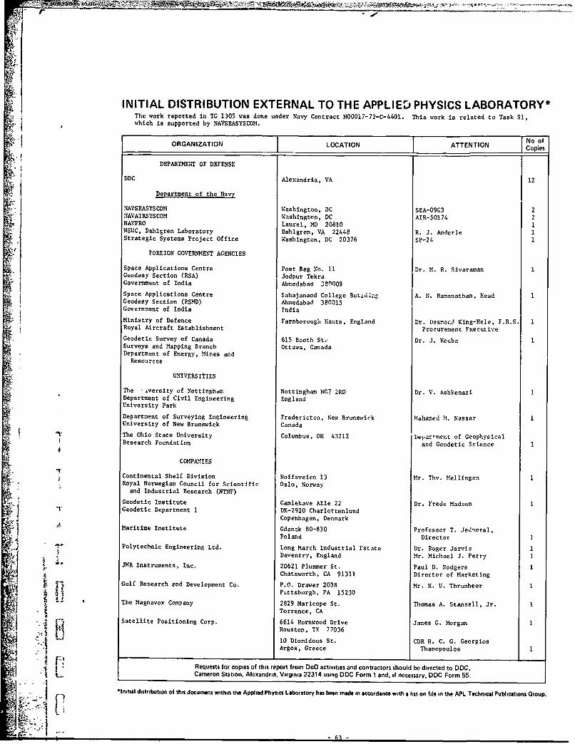
INITIAL DISTRIBUTION EXTERNAL TO THE APPLIED PHYSICS LABORATORY*-I i The work reported in TG 1305 was done under Navy Contract N00017-72-C-4401. This work is related to Task SI,

which is supported by NAVSEASYSCOM.

"ORGANIZATION LOCATION ATTENTION No of

ORGANIZATION Copies

DEPARTMEIT OF DEFENSE

DDC Alexandria, VA 12

Department of the Navy

NAVSEASYSCOM Washington, DC SEA-09G3 2I IAVAIRSYSCOM Washington, DC AIR-50174 2NAVPRO Laurel, MD 20810 1NSUC, Dahlgren Laboratory Dahlgren, VA 22448 R. J. Anderle 1Strategic Systems Project Office Washington, DC 20376 SP-24 I

FOREIGN GOVERNMENT AGENCIES

Space Applications Centre Post Bag No. 11 Dr. M. R. Sivaraman IGeodesy Section (RSA) Jodpur TekraGovernment of India Abmedabad 320009Space Applications Centre Sahajanand College Buildl.g A. N. Ramanathan, Head IGeodesy Section (RSMD) Ahmedabad 380015

Government of India India

Ministry of Defence Farnborough Hants, England Dr. DesnocA. King-Hele, F.R.S. 1Royal Aircraft Establishment Procurement FxecutiveGeodetic Survey of Canada 615 Booth St., Dr. J. Kouba 1Surveys and Mapping Branch Ottawa, CanadaDepartment of Energy, Mines and

Resources

UNIVERSITIES

The -iversity of Nottinghm, Nottingham NG7 2RD Dr. V. Ashkenazi 1Department of Civil Engineering EnglandUniversity Park

Department of Surveying Engineering Fredericton, New Brunswick Mahamed M. Nassar 1University of New Brunswick CanadaThe Ohio State University Columbus, OH 43212 Depar'ment of GeophysicalResearch Foundation and Geodetic Science 1

COMP&NIES

Continental Shelf Division Hoffsveien 13 Mr. Thv. Mellingen 1Royal Norwegian Council for Scientific Oslo, Norway

and Industrial Research (NTNF)

Geodetic Institute Gamlehave Alle 22 Dr. Frede Madsen IGeodetic Department 1 DK-2920 Charlottenlund

Copenhagen, DenmarkMaritime Institute Gdansk 80-830 Professor T. Jednoral,•1 Poland Director 1Polytechnic Engineering Ltd. Long March Industrial Fstate Dr. Roger Jarvis 1

Daventry, England Mr. Michael J. Perry 1

JMR Instruments, Inc. 20621 Plummer St. Paul D. Rodgers 1Chatsworth, CA 91311 Director of Marketing

Gulf Research end Development Co. P.O. Drawer 2038 Mr. H. U. Thrunheer 1Pittsburgh, PA 15230

The Magnavox Company 2829 Maricope St. Thomas A. Stansell, Jr. 1Torrence, CA

"Satellite Positioning Corp. 6614 Hornwood Drive James G. Morgan 1•.1 • Houston, TX 77036

• •. 10 Diomidous St. CDR H. C. G. Georgios"" Argos, Greece Thanopoulos IU Requests for copies of this report from DoD activities and contractors should be directed to DOC,

L Cameron Station, Alexandria. Virginia 22314 using DDC Form 1 and, if necessary. DDC Form 55.

linitil distribution of thes document within the Applied Physics Laboratory has been made in accordance with a list on file in the APL Technical Publications Group.

the transit system, 1975

Documents