The Trade Creating Effects of Business and Social Networks:

Evidence from France ∗

Pierre-Philippe Combes† Miren Lafourcade‡ Thierry Mayer§

June 22, 2004

Abstract

Using both standard and theory-grounded estimations of trade flow equations, the paperquantifies the role that business and social networks play in shaping trade between French regions.The bilateral intensity of networks is investigated using the financial structure and location ofFrench firms and bilateral stocks of migrants. Compared to a situation without networks, migrantsare shown to double bilateral trade flows. Moreover, the effect of migrants at the origin of thetrade flow is generally stronger than at its destination. Firm networks have even larger effects,multiplying trade flows by as much as five in some specifications. Besides providing the magnitudeof network effects, our results also support more the information-based impact of networks thanthe effects of imported preferences. Finally, we show that the role of usual proxies for tradeimpediments could be largely over-estimated when neglecting network effects. Taking them intoaccount reduces the estimated impact of transport costs by as much as 60% and divide the bordereffect by more than three.

JEL classification: F12, F15Keywords: migrants, business groups, networks, border effects, gravity, structural estimation.

∗We thank Jean-Eric Thomas for having kindly made the trade flow data available to us. We are also grateful toJohannes Brocker, Harry Flam, Laurent Gobillon, Keith Head, Christiane Krieger-Boden, and to seminar participants(ERWIT 2002, HWWA Workshop on border regions) for fruitful comments and discussions. Comments by JamesRauch and two anonymous referees were crucial in the improvement of the paper. The hospitality of the FrenchMinistry of Transport Economics Department (SES-DAEI) (Lafourcade’s PhD host) as well as financial support fromSES-DAEI and from NATO (Combes’ advanced fellowship grant) are gratefully acknowledged.

†CERAS-ENPC and Boston University. CNRS researcher also affiliated with the CEPR (combes@enpc.fr,http://www.enpc.fr /ceras/combes/).

‡Universite d’Evry Val d’Essonne (IUT - GLT Department) and CERAS-ENPC (lafourca@enpc.fr,http://www.enpc.fr/ceras/lafourcade/).

§Corresponding author: CERAS, 48 Bd Jourdan, 75014 Paris, France. Also affiliated with TEAM (Universite deParis I), CEPII and the CEPR (tmayer@univ-paris1.fr, http://team.univ-paris1.fr/trombi/mayer/thierry.htm).

1 Introduction

It is one of the most widely accepted results in international economics that trade is impeded by

distance, as testified by the large set of papers estimating standard gravity equations. A more recent

finding, initiated by McCallum (1995), is that, in addition to the impact of distance, the crossing of

national borders also sharply reduces trade.1 Furthermore, contiguity has also been largely shown

to have a positive impact on trade volumes. Hence, spatial proximity matters for trade, but in a

quite complex way that goes beyond the simple (log linear) impact of geographical distance. More

work is still needed to understand fully the reasons why these various notions of proximity matter so

much for trade. Obstfeld and Rogoff (2000) for instance refer to the border effect as one of the “six

major puzzles in international macroeconomics”. Although going a long way towards enlightening

this puzzle through a much improved link with theory, Anderson and van Wincoop (2003) are left

with non trivial “unexplained” trade impediments. In parallel, a recent strand of the literature

surveyed by Rauch (2001) and Wagner, Head and Ries (2002) suggests that business and social

networks operating across borders might promote trade notably through a reduction in information

costs. We try here to provide empirical evidence linking the two phenomena. This paper empirically

assesses the trade-creating effects of business and social networks and quantifies the share of trade

impediments (distance, borders, contiguity) that can be explained by those networks.

Networks can promote trade through different channels. The literature has proposed two main

economic mechanisms: The reduction of information costs and the diffusion of preferences. The

first channel relies on the potential alleviation of costs incurred by economic agents when gathering

information about distant markets. Indeed, informational barriers make it difficult both for con-

sumers to obtain relevant information on the goods produced in another location and for non-local

producers to learn the tastes of consumers or to be aware of the practices of local retailers. Both

effects increase transaction costs and thus perceived prices, which has a negative impact on trade

flows. The empirical work has used observed distributions of international migrants to identify this

effect. It is indeed likely that hosting a large number of migrants from other areas tend to pro-

mote trade because they keep active linkages with their networks at “home”: “Immigrants know the

characteristics of many domestic buyers and sellers and carry this knowledge abroad” (Rauch, 2001,

p.1184). Next to migrant effects, it has been suggested that networks of firms can also contribute

to alleviate information problems in the international marketplace, notably through foreign direct

investment.2 The fall of information costs inside networks also has an indirect positive effect on trade

working through better enforcement of contracts. Gould (1994) and Rauch (2001) detail how the

reciprocal knowledge of trade partners can help to reduce costly opportunism in business, networks

being substitutes of contract enforcement laws. Reputation effects are likely to be magnified inside

1Wei (1996), Helliwell (1996) and (1997), Nitsch (2000), Head and Mayer (2000), Anderson and van Wincoop (2003)and Chen (2003) are all examples of recent papers stating that the impact of national borders on trade volumes is allbut negligible among seemingly highly integrated countries.

2Rauch (2001) notably claims that “foreign direct investment by one or more members of a domestic business hasthe same effect [as the migrant effects]” (p.1185). More generally, strategic behavior inside networks of financially-linked enterprises might also affect trade patterns through subtle effects involving coordination and possible buildingof barriers to entry.

1

a network, due to the increased reciprocal knowledge and number of interactions across members

and the consequent higher speed of information flows. Rauch and Trindade (2002) also mention the

possible common enforcement of sanctions by the entire network against the deviating member as a

mean to deter violations of contracts and commitments.

The second channel for the impact of networks on trade is their role as a conduit for the diffusion

of preferences. Consumers may have a home bias that translates in a higher valuation for the goods

produced locally, either because of persistence in consumption habits inherited from a period where

markets where more fragmented or simply because of “chauvinism”. The presence of foreigners may

alter this tendency. Indeed a high number of migrants might raise imports from origin countries

both because migrants keep part of their taste for home goods and because nationals partly acquire

a taste for those new varieties. Presumably, the preference effect takes place for networks created

and maintained by individuals at the destination of the trade flow only (i.e. on imports). By

contrast, migrant networks at the origin of the trade flow (i.e. the impact of immigrants on exports)

and firm networks at both origin and destination should encompass information effects only. This

suggests several ways to disentangle between the information and preferences channels. Some papers

in the literature compare the effect of migrants on imports and exports so as to assess whether the

information channel is larger than the preferences one. Estimating the impact of networks of firms, as

done in this paper, makes it possible to go one step further (although not all the way) in this direction.

If the empirics reveal that networks of firms have a stronger effect than networks of migrants, it can

be interpreted as evidence of stronger informational effects within networks of firms, combined with

a level of preference effects sufficiently low to be overcome by the difference in information effects.

We use this new identification strategy in the paper.

Gould (1994), Head and Ries (2001), Girma and Yu (2002), Rauch and Trindade (2002) and

Wagner et al. (2002) illustrate the trade-creating effect of networks using estimates of migration

variables in gravity-type equations. The first three papers estimate the impact of migrants settled

in the United States, Canada and the United Kingdom respectively on national trade flows, while

Wagner et al. (2002) use information on the trade volumes of each Canadian provinces with a set of

foreign countries, coupled with the provincial stocks of migrants from each of those trade partners.

All papers find positive impacts of migrations on trade volumes with elasticities ranging from 0.01 to

0.31 (see Wagner et al., 2002, for a detailed comparative analysis of the papers). An interesting result

is that the effect of migrants is not shown to be consistently higher for imports than for exports.

As just highlighted, this casts doubt on the empirical importance of the preference channel, and

therefore supports the information channel. Rauch and Trindade (2002) strengthen this support in

their study of the impact of ethnic Chinese residents in origin and destination countries on the amount

traded by those countries. Their analysis mostly abstract from the preference channel because the

observations involving China as a trade partner are only a marginal part of the sample.3 One of their

key results is that networks between Chinese residents, when at the levels reached in South-East

Asian countries, increase trade by 60%. Additional evidence of the role of the information channel is

3The authors even control fully for this effect in a robustness check set of regressions that excludes Chinese trade.

2

provided through a distinction of the impact of networks across different types of goods, ranging from

most homogenous to most differentiated. The expectation is that for high levels of differentiation,

the need and efficiency of networks as information conduits should be magnified. While networks

appear to matter for all types of goods, the effects steadily increase with the differentiation of

products indeed, which confirms the intuition. Put together, the existing work on migration and

trade points towards a higher relevance of the information-related channels, a result we also find

some evidence of in this paper.

The empirical evidence related to the effects of networks of firms on trade is much scarcer than

the one on the trade impact of migration patterns. Most of the evidence relies on the particular

case of the links between member firms of Japanese keiretsus. Belderbos and Sleuwaegen (1998)

show that the share of production exported to the European Union by a Japanese electronic firm is

substantially higher if this firm is a component subcontractor in a vertical keiretsu and if the parent

firm has previously invested in the EU. A related empirical literature has shown that Japanese

imports are significantly lower in industries where a large share of sales is made by keiretsu members

(Lawrence, 1993, surveys early papers in this vein, while Head, Ries and Spencer, forthcoming, is

a recent application to the specific case of car parts). This last finding suggests that membership

of a keiretsu network facilitates trade between member firms at the expense of outsiders, although

it is unclear whether this effect comes from increased efficiency or exclusionary behavior. The most

important innovation of our paper consists in providing new and more systematic results on the

impact of networks of firms on trade and in comparing it to the strength of migrant ones.

More precisely, we estimate the trade-creating effects of business and social networks on inter-

regional trade flows between 94 French regions. The impact of social networks is quantified using

bilateral migrant stocks. Business network effects are assessed by using data on the links between

plants belonging to the same business group.4 Focusing on flows inside a given country helps to

isolate networks effects from other explanations of trade. In the same spirit as Wolf (2000) for the

United States, there can be in our framework no room for explanations based on trade policy or on

transaction costs associated with the use of different currencies, which both have been mentioned

as possible important trade impediments.5 We estimate standard gravity specifications of trade

flows, which facilitates comparisons with existing estimates of the impact of migrant networks. An

additional novel aspect of our work is the use of “structural” specifications directly derived from

a model of trade characterized by monopolistic competition, home-biased preferences, information

and transport costs. This approach, following recent advances in gravity-type equations, is designed

to reduce mis-specification and endogeneity issues. Within this vein, we present results along the

lines of the fixed-effects approach a la Hummels (1999) and Redding and Venables (2004) and two

different (though compatible) specifications based on Head and Mayer (2000) and Head and Ries

(2001).

Our estimates concerning the impact of migrants are close to those obtained in the literature.

4We use here the definition and terminology of the French National Institute of Statistics and Economic Studies(see Section 3 for more details).

5See Rose (2000), Parsley and Wei (2001) and Taglioni (2002) for recent empirical evidence.

3

Compared to a situation without networks, the average bilateral migrant population doubles trade

flows between French regions. The most important novelty in our results concerns the effect of

networks of firms. The links between plants belonging to the same business group multiply trade

flows by as much as five depending on the specification. Thus, the network effects of firms, working

through the information channel only, are notably higher than migrant ones. The generally higher

effects of migrants at the origin of the flow than at its destination is a further result of ours that

conforts the finding that information transmission would be the main mechanism at work in the

trade creating effects of networks. Finally, we show that the omission of network effects leads to

overestimate the trade depressing role of transport costs, administrative borders and non-contiguity.

The impact of transport costs on trade volumes is for instance reduced by as much as 60% when both

types of networks are controlled for. It is estimated that crossing administrative borders separating

French regions has the effect of dividing trade flows by two, while the same estimate is higher than

six without network controls.

The rest of the paper proceeds as follows. Section 2 presents the theoretical model and the

corresponding specifications to be estimated. The data used are described in Section 3. We separate

our results in two sections. Section 4 evaluates the trade creating effects of business and social

networks as estimated in specifications that consider only inter -regional trade flows and are thus

fully comparable with existing work. Section 5 introduces the trade impact of administrative borders

in the analysis. Using more sophisticated specifications, we quantify the impact of networks on all

trade impediments, whether related to transport cost, borders or contiguity. Section 6 concludes.

2 Theory and estimated specifications

We describe in this section the theoretical underpinnings of the empirical specifications of trade flows

we use. The modelling is inspired by the widely used trade model of monopolistic competition a la

Dixit-Stiglitz-Krugman (Dixit and Stiglitz, 1977; Krugman, 1980), slightly modified to account for

home bias in consumers’ preferences and transaction costs.6

2.1 Standard gravity and the fixed-effects approach

Consumption and trade flows

The representative consumer’s utility in region i depends upon the consumption cijh of all varieties

h produced in any region j. Varieties are differentiated with a constant elasticity of substitution

(CES) but they do not enter symmetrically the utility function: A specific weight, aij , is attached to

all varieties imported from region j, describing preferences of i consumers with respect to j varieties.

Let nj denote the number of varieties produced in region j and N the total number of regions. The

6Feenstra (2003) presents a complete overview of theoretical foundations and empirical applications of the grav-ity equation mainly focused on the monopolistic competition framework. Anderson and Van Wincoop (2003) andEaton and Kortum (2002) are examples of alternative theoretical frameworks that also lead to gravity-type structuralestimations of trade flows.

4

corresponding utility function is

Ui =

N∑j=1

nj∑h=1

(aijcijh)σ−1

σ

σσ−1

, (1)

where σ > 1 is the elasticity of substitution. Let pij denote the delivered price in region i of any

variety produced in region j. Denoting by τij the iceberg-type ad-valorem equivalent transaction

cost between regions j and i and pj the mill price in j, we have pij = (1 + τij) pj . It is then

straightforward to obtain the following demand function

cij = ciPσi njp

−σj aσ−1

ij (1 + τij)−σ , (2)

where ci =∑

j

∑h cijh is total consumption (in quantities7) in region i of differentiated good varieties

imported from all possible source regions (including i) and where Pi is the price index in region i,

Pi ≡(∑

j aσ−1ij njp

1−σij

)1/(1−σ).8

Equation (2) links imports of region i from region j to the size of the demand expressed by the

destination region i (ci), and its price index (Pi), the size of the supply (nj) and the mill price (pj)

of the origin region j, and bilateral effects involving preferences (aij) and transaction costs (τij).

There are two major problems that must be solved in order to obtain an estimable specification

from equation (2). One must first deal with Pi, which complicates the estimation by introducing

non linearity in unknown parameters. Next, the number of varieties produced in region j, nj , and

the delivered prices, pij , are usually not accurately measured and sometimes simply unobservable.

We consider four alternative strategies to tackle these issues. The most usual approach more or

less ignores these problems, merely expecting that they will be of secondary order in the estimation,

trade flows being overwhelmingly determined by the size of partners and a set of transaction costs

proxies. This corresponds to the standard gravity specification. Considering this type of specification

is interesting as it gives a benchmark set of results enabling comparisons with the existing literature.

The second approach establishes a closer link with theory. Equation (2) involves three groups of

variables: Origin (j-specific), destination (i-specific) and “dyadic” (or bilateral ij-specific) variables.

When mostly interested in coefficients on dyadic variables, as is the case here, a theory-consistent

specification of equation (2) uses fixed effects, for origin and destination regions, to capture the first

two groups of variables. This is the fixed-effects approach notably used by Hummels (1999) and

Redding and Venables (2004) in similar theoretical settings.

Last, we use two approaches which go further in the use of the theoretical framework to derive

the specifications to be estimated. We call those the odds and friction specifications respectively.

Presenting the details of these approaches will be easier after the specification of transaction costs

(τij) and of consumers’ preferences (aij).

7Those equations are usually presented in terms of the bilateral value of trade flows (equation 2 times pij). Wework with trade flows in tons in the empirics and accordingly present the equations in quantity terms.

8Note that, with a production function a la Ethier (1982), the demand for inputs and therefore trade flows inintermediates take the same functional form, which is important as this type of shipments is a large share of totaltrade.

5

Transaction costs and preferences

We consider two different elements in transaction costs: Physical transport costs, Tij , and informa-

tion costs, Iij . We model transaction costs as follows:

1 + τij = TijIij . (3)

Transport costs are assumed to have the structure

Tij = (1 + tij)δ exp(−θ(1 + tij)2), (4)

where tij is a measure of transport cost between i and j (detailed in section 3). With this specifica-

tion, the absence of transport costs (tij = 0) would yield Tij = 1, which means that transaction costs

would be entirely caused by information issues. Parameters δ and θ are expected to be positive.

The quadratic cost function chosen embodies a standard feature of increasing returns in transport

activities: The marginal cost of shipping a good is positive but it decreases with distance.

For the information cost, we assume

Iij = (1 + migij)−αI (1 + migji)

−βI (1 + plantij)−γI (1 + plantji)

−ρI exp (ϕIAij − ψICij) . (5)

Aij is a dummy variable set to 1 when i 6= j and Cij is another dummy set to 1 when i and

j are contiguous (but still different) regions. Our hypothesis is that ϕI > 0 and ψI > 0: The

informational transaction cost is lower inside a region than between two regions, but higher between

two non-contiguous regions than between contiguous ones.

The impact of business and social networks on information costs is captured by four variables,

migij , migji, plantij and plantji corresponding to migrant and plant networks. Origin and destination

subscripts of mig variables are chosen so that the historical movements of people underlying those

variable follow the same direction as trade flows. Since cij is the trade flow going from j to i, migij is

the number of people born in region j and working in region i, which corresponds to the cumulated

flow of people that moved from j to i at some point in time and are still located there. We refer

to the effect of migij as the “migrants at destination” effect. Reciprocally, migji is the “migrants

at origin” effect. Note the correspondence with the existing work on migration and trade surveyed

in the introduction. We work here with a single trade matrix and two migration variables, whereas

most of the existing work isolates imports from exports and thus uses two trade matrices but only

one migration variable (estimating the impact of inward migration on imports and exports). The

two approaches rely however on the same two effects: migij is here the effect of inward migrations

on imports and migji the effect of inward migrations on exports.

Following the same logic concerning origin and destination subscripts, let plantij denote the

number of plants located in the importing region i that belong to the same business group as at

least one plant in region j. This variable is labeled the “plants at destination” effect and conversely

for the “plants at origin” effect, plantji. The four network variable labels therefore indicate where

the agent (whether migrant or plant) is located, at the origin or at the destination of the flow. As

6

stated in the introduction, migrant and plant networks are assumed to reduce information costs of

trade shipments going both directions. Parameters αI , βI , γI and ρI are therefore all expected to

be positive.

Consumers are assumed to have both deterministic and stochastic elements in their preferences,

aij . We assume systematic preferences for (i) local goods (produced in the region of consumption),

(ii) goods produced in a contiguous region, and (iii) goods produced in the region where the consumer

was born. This last effect is assumed to be increasing in the migrants at destination variable, migij :

Migrants partly bring their preferences for home products with them in the destination region and

this pattern possibly propagates to the local consumers, raising the level of imports of the host

region. Last, the random component in the preferences is denoted eij , and we assume the structure

aij = (1 + migij)αa exp[eij − ϕaAij + ψaCij ], (6)

on preferences, with αa, ϕa and ψa being parameters, all expected to be positive. Migrants at des-

tination can therefore have an effect on trade through both preference and information channels.

Note that the effects are fundamentally different in both cases. For the preference part, the impact

of migration corresponds to exogenous effects directly affecting the preferences of consumers. Con-

cerning informational costs, they correspond to endogenous demand effects working in equilibrium

through delivered prices that increase with transaction costs.

We now proceed to a presentation of the exact specifications that will be estimated and show

how they relate to the theoretical expression of trade flows given in equation (2), combined with

the specifications of transport costs (equation 4), information costs (equation 5), and preferences

(equation 6).

The gravity specification

The gravity specification has the weakest links with theory. Our data allow a computation of

the destination consumption (ci), which reflects the role of the size of the destination economy in

equation (2). Next, the size of the origin economy (the number of firms/varieties, nj , in equation 2) is

proxied by the value of the production, which we denote by vj . The elasticities for these two variables

are usually assumed to be identical. In fact, theory even suggests that both coefficients should be

unitary. Gravity equations also often incorporate remoteness variables (see Wei, 1996, or Frankel,

1997, for instance), for which the link with theory is at first sight even fuzzier. Those terms are in

fact a way to capture the price terms in equation (2) as is made clear in Wei (1996) and Anderson

and van Wincoop (2003). The price index of region j is often proxied by the remoteness variable

remj =∑

k 6=jdjk

vk. This is admittedly a crude approximation of the true underlying theoretical price

index(Pj =

[∑k a

σ−1jk nkp

1−σjk

]1/(1−σ))

, capturing the fact that a region where competition is fierce

(and hence where the price index is low because of its geographic centrality) is – everything else

equal – harder to penetrate. Again, remoteness variables should have the same, positive, coefficient

(see the theoretical developments of Wei, 1996 and Anderson and van Wincoop, 2003). Following a

7

large part of the gravity equation literature (Rauch and Trindade, 2002, and Rose 2000, are recent

examples), we estimate size and remoteness effects using the product of each couple of variables

(ci × vj and remi × remj respectively). To be as close as possible to usual gravity specifications, we

also consider the effect of contiguity, and drop the observations for trade flows taking place inside

each region, cii, which are re-introduced in section 5. We also proxy the transport cost by the

geographical distance between the main city in each region (dij)9 and drop the quadratic term in

the transport cost specification (equation 4). Using the structure specified above for the impact of

networks on preferences and information costs, and using the notations x ≡ σxI + (σ − 1)xa for

x = α and ψ, and y ≡ σyI , for y = β, γ and ρ, the gravity specification is given by:

ln (cij) = a1 + a2 ln (ci × vj) + a3 ln (remi × remj)− a4 ln (dij) + ψCij

+α ln(1 + migij

)+ β ln

(1 + migji

)+ γ ln

(1 + plantij

)+ ρ ln

(1 + plantji

)+ εij , (7)

where a1 to a4 are parameters that should be positive according to theory. Unfortunately, these

parameters cannot be linked to structural ones, the covariates used being too far from those implied

by theory. Strictly speaking, α, ψ, β, γ and ρ are notations that should also be reserved to structural

estimation of the theoretical model, but we use them here too, in order to keep notation simple.

The fixed-effects specification

In the spirit of Hummels (1999) and Redding and Venables (2004)10, it is possible to derive from

equation (2) a fixed-effects specification fully consistent with the theoretical model, contrary to

the gravity specification. The idea consists in replacing all destination-specific and origin-specific

variables by two groups of destination and origin fixed-effects. Only dyadic variables are then left

in the regression. As for the gravity specification, we try to stay here as close as possible to the

specifications estimated in the literature. We drop internal trade flows (no border effects), and

continue to use a simple log-linear effect of distance as a proxy for transport costs. This leads to the

fixed-effects specification given by:

ln (cij) = fi + fj − b1 ln (dij) + ψCij

+α ln(1 + migij

)+ β ln

(1 + migji

)+ γ ln

(1 + plantij

)+ ρ ln

(1 + plantji

)+ εij . (8)

where fi and fj are destination– and origin–region fixed effects respectively and b1 is an extra

parameter to be estimated. The main drawback of this approach is that it does not allow to estimate

all structural parameters. In particular, the elasticity of substitution between varieties (σ), which

has been the subject of important academic interest in this type of analysis recently, cannot be

recovered.

9We do not consider geodesic distance here, but real road distance.10Harrigan (1996) seems to be one of the first to have used fixed effects in the estimation of a monopolistic competition

model of bilateral trade flows.

8

2.2 The odds and friction specifications

We now present specifications that permit broader identification of parameters. This requires to

use theory further and makes use of a convenient feature of CES demand functions, emphasized in

Anderson, de Palma and Thisse (1992) and often called the Independence of Irrelevant Alternatives

(IIA) due to its similarity with the logit model. With this type of demand structure, the ratio of

two bilateral trade flows to a same destination depends only on the characteristics of the two origins,

which greatly simplifies the specification.11

The Production Side of the Model

Let r denote a reference region. When imports of region i from region j are divided by imports of

region i from region r (equation 2), one gets:

cijcir

=(aij

air

)σ−1(1 + τij1 + τir

)−σ (pj

pr

)−σ (nj

nr

). (9)

While the price index does not enter the equation anymore, one still has to deal with numbers of

varieties and mill prices. It is possible, however, to use the behavior of producers under monopolistic

competition to obtain a correspondence with variables that are easier to observe, namely regional

production and wages. As usual in this type of model, it is assumed that differentiation costs are

sufficiently low to ensure that each variety is produced by a single firm with an increasing returns

to scale technology common to all regions and using labor as the only input.

The Dixit-Stiglitz-Krugman model of monopolistic competition assumes that firms are too small

to have a sizeable impact on the overall price index and on the regional income, when they set their

price to maximize profits. This yields the standard constant markup over marginal cost pricing rule,

pj = σσ−1gwj , where wj is the wage rate in region j and g the unit labor requirement. Consequently,

all varieties produced in region j have the same mill price. The zero profit condition gives the

equilibrium output of each firm, which is the same in all regions, and will be noted q. Let vj denote

the value of the total production in region j, we obtain vj = njpjq. Therefore, using the pricing rule,

nj/nr = (vjwr)/(vrwj). Using the definition of the delivered prices and the pricing rule, equation (9)

can be rewritten ascijcir

=(aij

air

)σ−1(1 + τij1 + τir

)−σ (wj

wr

)−(σ+1) vj

vr. (10)

11The main interest of this approach is to solve the issue of the highly non linear price index term in estimation. Headand Mayer (2000) and Eaton and Kortum (2002) also use this property of the CES function to obtain their estimabletrade equation. Lai and Trefler (2002) and Anderson and van Wincoop (2003) have different empirical approaches ofthe same issue involving non linear estimation techniques.

9

The odds specifications

Replacing in equation (10) the different specifications we assume for the transaction cost (equations 3

to 5) and the preferences (equation 6), we obtain what we call the odds specification

ln(cijcir

)= φ ln

(vj

vr

)− (σ + 1) ln

(wj

wr

)− σδ ln

(1 + tij1 + tir

)+ σθ

[(1 + tij)2 − (1 + tir)2

]+α ln

(1 + migij

1 + migir

)+ β ln

(1 + migji

1 + migri

)+ γ ln

(1 + plantij

1 + plantir

)+ ρ ln

(1 + plantji

1 + plantri

)−ϕ (Aij −Air) + ψ(Cij − Cir) + εij , (11)

where ϕ ≡ σϕI + (σ − 1)ϕa. The fact that εij = (σ − 1)(eij − eir) implies that errors are not

independently distributed. This correlation is accounted for in the estimation through a robust clus-

tering procedure, allowing residuals of the same importing region to be correlated. The theoretical

framework predicts φ = 1. φ is a parameter introduced here in order to give additional flexibility in

the estimations. The results regarding the impact of business and social networks are virtually un-

affected by this standard variant of the model. Furthermore, we propose below another specification

that bypasses the estimation of the coefficient on production.

We actually estimate two different odds specifications. The complete odds specification takes

the internal flow or “imports from self” as a reference, that is, it assumes r = i in equation (11).

This amounts to dividing each inter-regional flow by the corresponding internal flow of the importer.

Then, since only the i 6= j observations are kept in the regression, −ϕ (Aij −Aii) = −ϕ, which is

the constant of the model and provides an estimate of the effect of administrative borders on trade

volumes in France. The complete odds specification is:

ln(cijcii

)= φ ln

(vj

vi

)− (σ + 1) ln

(wj

wi

)− σδ ln

(1 + tij1 + tii

)+ +σθ

[(1 + tij)2 − (1 + tii)2

]+α ln

(1 + migij

1 + migii

)+ β ln

(1 + migji

1 + migii

)+ γ ln

(1 + plantij

1 + plantii

)+ ρ ln

(1 + plantji

1 + plantii

)−ϕ+ ψCij + εij . (12)

In order to fill – or at least shorten – the gap between the estimations of the gravity and the

fixed-effect specifications on the one hand and those coming from the complete odds specification on

the other hand, we also estimate what we call the basic odds specification that does not use internal

trade flows (and thus does not consider border effects). For each destination i the reference region

(r in equation 11) is chosen to be the origin region with the largest flow to region i.

The friction specification

Finally, following Head and Ries (2001), we estimate a specification which goes one step further in

using the IIA property of the CES. An inverse index of “frictions” to trade, often referred to as a

10

freeness of trade index, can be defined as

Φij =√cijcii

cjicjj. (13)

Using equation (12), and assuming that tij = tji, we obtain the friction specification:

ln (Φij) = −σδ ln

(1 + tij√

(1 + tii)(1 + tjj)

)+ σθ

[(1 + tij)2 −

12(1 + tii)2 −

12(1 + tjj)2

]

+(α+ β) ln

(√(1 + migij)(1 + migji)(1 + migii)(1 + migjj)

)+ (γ + ρ) ln

(√(1 + plantij)(1 + plantji)(1 + plantii)(1 + plantjj)

)−ϕ+ ψCij + εij . (14)

The friction specification has the advantage of being compatible with the strict version of the

model implying φ = 1. Importantly, it does not require data on regional values of production (vi)

and wages (wi), which is a noticeable advantage considering the measurement errors and missing

values often found in those series as well as the likely endogeneity issues associated with these

variables. Again, autocorrelation introduced by the fact that εij = 12(εij + εji) is taken into account

in estimation.

2.3 Identification issues

As detailed above, the impact of networks can reflect two broadly defined underlying economic

mechanisms: Reductions in trade-related information costs on the one hand (and the associated fall

in opportunistic behavior), and diffusion of preferences on the other hand. The two mechanisms

have different implications and it is an attractive goal to identify which is the most relevant.

Unfortunately, none of our five specifications allows for an identification of all structural pa-

rameters associated with business and social networks. Take the simplest case of the gravity equa-

tion (7). The estimation gives, as in all specifications used here except friction, α ≡ σαI +(σ−1)αa,

ψ ≡ σψI + (σ − 1)ψa, β ≡ σβI , γ ≡ σγI , and ρ ≡ σρI .

Note first that the information effects in the transaction cost cannot be distinguished from the

preferences effects in α. It is however possible to assess the relative strength of the information and

preference channels in migrant networks by comparing α and β. If one is willing to accept that the

information about trade opportunities conveyed by migrants is similar in the two trade directions,

αI ≈ βI , then α − β ≈ (σ − 1)αa, which is the pure preference effect. This is exactly what Gould

(1994), Girma and Yu (2002) or Wagner et al. (2002) assume when they compare the impact of

immigrants on imports and exports. When the actual implementation of this method gives α−β < 0

(as happens quite frequently in the literature as well as here), it can be concluded that the effect

of preferences is sufficiently weak to be dominated by the information effect of migrants on exports,

even when the information effect on imports is added to preferences.

As stated in the introduction, it seems also possible to use the fact that networks of plants

convey information gains only, while migrants (at destination) additionally incorporate the effect of

11

preference diffusion on trade to distinguish between the two effects from estimated parameters. This

is however only possible if the information effect has the same strength in the two type of networks.

Consider the difference between the two ij network variable parameters: α−γ = σ(αI−γI)+(σ−1)αa.

If the information effects are exactly the same, αI − γI = 0, and the difference between the two

coefficients gives the pure preference effect. In general however, there is no reason to believe that

αI = γI .12 As with the comparison of the two migrants coefficients, a result of α − γ < 0 (which

is what we generally obtain here) means that the pure information effect of plants (σγI) dominates

the combined effect of information and preferences by migrants (σαI + (σ − 1)αa).

Note finally that even less information on network parameters can be retrieved from the friction

specification (14). Only α + β, and γ + ρ are identifiable. This is the drawback of a specification

that offers nevertheless the important advantage of less (potentially noisy) data collection needs and

of reduced endogeneity concerns (see Section 5).

3 Data

The data needed to estimate the specifications just described consist in bilateral trade flows, regional

production and wages, bilateral measures of transport costs and of business and social networks. Our

sample covers trade between and within French regions for the year 1993. Regions are defined ac-

cording to the administrative division of continental France into 94 units called “departements”. The

spatial organization of France in departements was introduced simultaneously with the elaboration

of the first French constitution (there were 83 departements in the original bill voted in 1790). Inter-

estingly, the original design of this key reform of French administration accompanying the change of

political regime was concerned with economic motivations, and more precisely transportation issues:

The size of each departement would have to be such that it would be possible from any point inside

the departement to reach its capital city (usually centrally located) and come back within 48 hours.

This meant, at a time when horses were the fastest mean of transport, departements organized

within a radius of 30 to 40 kilometers around their capitals.

Even today, departements probably represent meaningful lines of demarcation inside France for

both economic activity and networks. One of the reasons for this is that departements have been

given important attributions, with corresponding budgetary transfers, by the “decentralization laws”

of 1982-1983.13 The central government provided the financial means of this policy through (i) the

direct funding of each departement’s budget and (ii) through transfers of direct and indirect local

tax instruments on which the departement has full authority (this part represents the majority of

receipts in the budget of departements, see Ministry of the Interior (DGCL), 2003, for details). The

12Following the logic of Rauch and Trindade (2002), it seems possible to find sufficiently homogenous products sothat αI ≈ γI ≈ 0. This raises new questions, however. First, Rauch and Trindade (2002) find that the informationchannel still matters for their most homogenous goods. Second, such homogenous goods should be the ones where thepreference channel is also negligible (αa ≈ 0), rendering the identification procedure meaningless.

13The most important of those attributions concern social aid actions, the construction and operation costs of the4 first years of secondary schools (“colleges”, with the exception of personnel salaries), and the construction andmaintenance costs of part of the roads (a substantial part in rural areas).

12

elected executive power of each departement thus has a substantial impact on the local economy

through its fiscal and tax policies.14 In parallel, business and social networks are likely to be at least

partly organized around the natural delimitations that departements represent. Although it is hard

to capture precisely something like the density and spatial extent of networks, an example of this

phenomenon is the spatial organization of the chambers of commerce and industry in France. Each

departement has usually one such chamber (the departements with the largest cities or industrial

bases have usually two), taking the name of the departement. Those chambers have the official role of

representing the “commercial and industrial interests of their jurisdiction” to the public authorities

and are elected by the local business community. They notably provide services to local firms in

terms of administrative procedures for the creation of a firm, data and expertise on local markets

and potential suppliers, relationships with local authorities. They are consulted in the making of

local public policies on numerous economic-related subjects. Moreover, those chambers officially

administrate 121 airports, 180 ports, more than 300 educational establishments (and notably a

large number of business schools) and 55 exposition halls (ACFCI, 2002). These institutions are an

example of why departments can constitute relevant geographical units for the establishment and

maintenance of networks in France.

Trade, production and wages

Trade flows between and inside regions come from the French Ministry of Transports database on

commodity flows. The source and construction method of these data are comparable to the U.S.

Commodity Flow Survey (CFS) recently used in Wolf (2000), Anderson and van Wincoop (2003) or

Hillberry and Hummels (2003) for instance. The data is based on an annual survey of a stratified

random sample of vehicles from the road transport industry to which the exhaustive collection of

trade flows shipped by railway is added.

The dataset includes both inter- and intra-regional flows and is originally available at a very

detailed industry level. However, the number of observations being low for some industries, we

aggregate the flows over all industries. This data set suffers from the same imperfections as the CFS

concerning the way loading and unloading are handled. The main issue is the statistical collection

of actual origins and destinations of shipments that transit through warehouses or ports for instance

where they are unloaded and later re-loaded on an often different truck or mode. Those issues

can result in a distorted image of actual trade patterns. It has been notably shown by Hillberry

and Hummels (2003) that shipments originating from wholesalers cover a much lower distance that

shipments from manufacturers, reflecting hub and spoke arrangements in distribution. Those short-

distance flows from wholesalers to retailers contribute to inflate the amount of trade taking place

within the administrative borders of American states and their estimated trade-reducing effect.

Besides, while both the CFS and our dataset try to sort out flows that are only in transit in a region,

a large amount of shipments to and from major ports is admitted to be in reality transit shipments.

14The overall fiscal expenditures of departements in 2003 are around 47 billion euros against a predicted 273 billionsfor the French central government.

13

The corresponding origin region then appears to be an excessive source of flows compared to its

real production (and reciprocally as destination). One way, consistent with theory, to mitigate this

problem is to consider regional production (computed as the sum of the flows departing from the

region including the internal flow) instead of GDP as the origin size variable. Similarly, the size of

the destination region can be computed as the sum of all flows to the region instead of the regional

GDP.15 The fixed-effects approach is another way to account for those transit flows since the dummy

variable for a given region will capture the fact that this region appears to import or export too

much compared to its GDP. Last, labor costs are proxied by dividing the annual regional wage bill

by the regional number of workers. This computation uses the “Enquete Annuelle d’Entreprises”

survey (EAE) from the French National Institute of Statistics and Economic studies (INSEE).

Distance and transport costs

The theoretical model requires the use of a measure of transport costs between and within French

regions. Most studies investigating trade determinants use great circle distance as a proxy for those

costs. In order to make the comparison with previous papers easier, our gravity, fixed-effects and

basic odds specifications are also estimated using distance, but real road distance between the main

cities of the two partner regions.

For the complete odds and the friction specifications, we follow a recent trend in the literature

that uses newly available data on actual transport costs (see for instance Hummels, 1999, Limao

and Venables, 2001). We use the Combes and Lafourcade (2003) data set that provides the cost for

a truck to connect each pair of French regions. This generalized transport cost includes both a cost

per kilometer (gas, tolls,...) and a time opportunity cost (drivers’ wages, insurance,...), and therefore

accounts for both distance and time-related transport costs (see Combes and Lafourcade, 2003, for

more details). The estimation of the complete odds and friction specifications also requires an intra-

regional transport cost for which no data exist in France. We construct those by first regressing

transport costs on real road distances and then applying estimated coefficients to internal distances

in order to obtain the corresponding internal transport costs. The internal distance is obtained using

the standard approximation that each region is a disk upon which all production concentrates at the

center and consumers are uniformly distributed throughout a given proportion of the total land-area

of the region. We choose this proportion to be equal to 116 , which is a reasonable approximation of

the observed concentration of population in France.16 The internal distance formula is thus given

by dii = 1/6√A/π = 0.094

√A where A is the regional land-area.

15Results using GDPs are available upon request. Our primary interest results, coefficients on network effects, arevirtually unaffected.

16INSEE (2001) reports that more than 80% of the French area was occupied by agricultural land in 1999 and that77% of the population lived in urban areas. The impact of alternative choices for the internal distance are discussedin section 5.

14

Business and social networks

The migrant network variables correspond to the number of people working in the destination region

who were born in the origin region (and the reverse). They are thus bilateral stock variables computed

using the Declaration Annuelle the Donnees Sociales survey (DADS) collected by the French National

Statistical Institute, INSEE. The plant network variables correspond to the number of plants located

in the destination region belonging to a business group which has at least one other plant located

in the origin region (and the reverse). A business group has a larger definition than a firm (itself

potentially incorporating several plants). For instance, all plants of the two car-producing firms

Peugeot and Citroen belong to the same business group called PSA. The precise definition of a

business group is the set of firms controlled directly or indirectly by a given firm, itself not controlled

by any other. The definition of control is the ownership of more than 50% of the votes in the

shareholders’ committee. Both types of network variables (four in total) are calculated using 1993

data, the same year as trade flows.

The DADS survey includes a representative 1/24th of the French population (all French citizens

born in October of even years, see Abowd, Kramarz and Margolis, 1999, for a detailed description

of this data). Table 1 gives summary statistics for the data we use. Since the average of the migrant

variables in the DADS survey is around 29, we approximately expect an average of 700 persons born

in a given region and living in another one. This corresponds to an average share of migrants in

region i born in region j around 0.5%. Correspondingly, it is possible to compute that the share of

people still working in the region where they were born is on average 52.6%.

In the average departement, 64 plants have at least one business group connection with any single

other region. The spatial variability of plant networks is lower than that of migrant networks. It

can also be computed that the number of plants having at least another plant belonging to the same

business group located in the same region is 229. Thus, as for migrant networks but to a smaller

extent, plant networks present the feature of much higher values for intra-regional observations: A

ratio of 3.6, against more than 100 for migrations. This can be usefully compared to the fact that

the average intra-regional flow is more than a hundred times larger than the inter-regional average

flow (8220683 against 68883 tons).17

Table 2 presents the simple correlations between all variables. The correlations between flows

and network variables are large. Flows, and migrant networks, are also strongly negatively correlated

with distance or transport costs. As explained in Combes and Lafourcade (2003), the correlation

between bilateral distance and transport costs is very high. Last, a positive correlation between any

two network variables is also observed. This is particularly the case for plant networks for which

this correlation is quite high.

Figure 1 helps further the understanding of these correlations and, more generally, of the spatial

patterns of network variables. The left-hand side maps correspond to the migrant networks and

the right-hand side to the plant ones. Each pair of maps corresponds to one of the destination

17Note also that the average flow inside a department is higher than the maximal flow between two different regionsin our sample.

15

Table 1: Summary Statistics

Variable Mean Sdt. Dev. Min Maxflows (tons) 68883 221971 1 8012491production (1000 tons) 14600 9072 1367 49800consumption (1000 tons) 14500 8762 2169 47800wages (1000 ECUs/year) 23.1 2.1 20.1 33.0distance (kms) 459.2 229.3 11 1282transport costs (French francs) 2666.6 1206.7 290.2 6966.8migrants at destination (# persons) 28.8 141.3 0 7332migrants at origin (# persons) 28.7 141.3 0 7332plants at destination (# plants) 64.3 72.0 0 651plant at origin (# plants) 64.3 72.0 0 651

Note: Statistics calculated for the sample used in section 4 and consisting of inter -regional flows only (omitting the 94 observations where i = j). The constructionof the migrant (plant alternatively) network variables implies that variables atorigin and at destination have identical distributions since each ij observationhas a corresponding ji one taking the same value. The mean values are notexactly identical here however since only non-zero inter-regional trade flows arekept, which excludes 14.8% (1251/8742) of the observations and makes the sampleslightly asymmetric.

Table 2: Correlation matrix

(1) (2) (3) (4) (5) (6) (7) (8) (9) (10)flows (1) 1 0.18* 0.17* 0.09* -0.33* -0.34* 0.42* 0.45* 0.28* 0.27*production at orig. (2) 1 -0.05* 0.31* 0.12* 0.10* 0.07* 0.08* 0.54* 0.29*consumption at dest. (3) 1 -0.02 0.11* 0.09* 0.09* 0.08* 0.31* 0.54*wages at orig. (4) 1 -0.02 -0.04* 0.16* 0.26* 0.60* 0.27*distance (5) 1 0.99* -0.18* -0.18* -0.03* -0.03transport costs (6) 1 -0.18* -0.18* -0.05* -0.05*mig. at dest. (7) 1 0.44* 0.32* 0.33*mig. at orig. (8) 1 0.33* 0.32*plant at dest. (9) 1 0.74*plant at orig. (10) 1Note: * denotes significantly different from 0 at the 1%level.

16

departement hosting the three largest French cities: Paris (top pair), Rhone (Lyon, middle pair) and

Bouches-du-Rhone (Marseille, bottom pair). For each map, the highest class is colored in black and

only includes the region to which the map refers, which facilitates its location.

The top left map shows that Paris hosts large numbers of migrants originating from regions either

relatively proximate to Paris (North, North-West of France), or more remote but larger in terms of

population (the regions hosting Bordeaux, Lyon and Marseille notably). This gravity pattern also

clearly emerges for Rhone and Bouches-du-Rhone. The effect of distance is still strong but large

regions as Paris or Nord appear as major sources of migrants. Regarding plant networks, the impact

of distance is less striking. The size of the origin region, however, still has a clear role, the spatial

pattern of plant networks being quite similar independently from the destination region. Levels

change, however. This conclusion is confirmed by the high correlations between plant variables and

production (see Table 2).

4 The trade creating effect of business and social networks

This section evaluates the statistical significance and economic magnitude of the impact of business

and social networks on trade flows. Results are presented omitting intra-regional trade observations,

and therefore abstracting from the analysis of border effects, covered in the next section.

Significance of network variables

Tables 3, 4 and 5 report the estimations for the gravity, the fixed-effects and the basic odds speci-

fications, respectively. The structure of these tables is the same. Column (1) reports the estimates

without network variables. Migrant effects are introduced one by one in columns (2) and (3) and

simultaneously in column (4). Columns (5) to (7) proceed similarly with plant networks. Last,

column (8) reports results considering all network effects together.

Table 3 reveals standard and expected results on traditional gravity variables. The coefficient

on the size variable is almost unitary, remoteness and contiguity have the expected positive impact

on trade flows, and bilateral distance strongly impedes trade.18 All those coefficients are extremely

precisely estimated, and the overall fit of the regression is within the usual (high) range for gravity

equations. Concerning the network effects we are primarily interested in, a first overall conclusion

to be drawn from Tables 3, 4 and 5 is that the impact of business and social networks is consistent

with theoretical predictions and qualitatively similar in all specifications used. When introduced

separately, all network variables have a positive and very significant impact on trade flows in the

three specifications. When all network variables are simultaneously introduced (in columns 8 of the

three tables), they sometimes exclude each other. Two of them are not significantly different from

18The estimated impact of distance is larger (in absolute value) than usually found. A plausible explanation isthat our sample exclusively incorporates flows transiting through ground transport means, which has been shown byDisdier and Head (2003) to yield substantially higher distance coefficients. They show in a meta-analysis of distancecoefficients in gravity equations that papers involving countries belonging to a single continent have distance coefficientabout 0.4 above the average distance effect estimate. Note also that the distance coefficient gets back to more usualvalues (around minus unity) when using the basic odds specification.

17

Figure 1: Number of Migrants (left) and Number of Plants Connected (right), for Paris (top), Rhone(middle) and Bouches-du-Rhone (bottom)

18

Table 3: Gravity specification

Dependent variable: FlowModel : (1) (2) (3) (4) (5) (6) (7) (8)intercept -3.64 -2.46 -2.76 -2.07 -1.94 -0.16 -0.29 -0.54

(2.78) (2.67) (2.77) (2.64) (2.88) (2.64) (2.71) (2.69)product size 0.93a 0.84a 0.89a 0.83a 0.85a 0.77a 0.77a 0.76a

(0.05) (0.05) (0.05) (0.05) (0.06) (0.05) (0.05) (0.05)product remote 0.61a 0.56a 0.61a 0.56a 0.58a 0.56a 0.56a 0.55a

(0.11) (0.10) (0.11) (0.10) (0.10) (0.10) (0.10) (0.10)distance -1.73a -1.61a -1.69a -1.59a -1.70a -1.67a -1.67a -1.60a

(0.06) (0.08) (0.06) (0.08) (0.06) (0.06) (0.06) (0.07)contiguity 1.04a 0.87a 0.97a 0.85a 1.05a 1.06a 1.05a 0.92a

(0.07) (0.07) (0.07) (0.08) (0.07) (0.07) (0.07) (0.08)migrants dest. 0.14a 0.13a 0.09a

(0.03) (0.03) (0.03)migrants orig. 0.05b 0.03 0.02

(0.02) (0.02) (0.03)plants dest. 0.11a -0.02 -0.03

(0.03) (0.05) (0.05)plants orig. 0.20a 0.22a 0.15a

(0.04) (0.05) (0.05)N 7491 7491 7491 7491 7491 7491 7491 7491R2 0.545 0.549 0.546 0.549 0.546 0.549 0.549 0.551RMSE 1.388 1.382 1.388 1.382 1.387 1.383 1.383 1.381Notes: (i) All variables in logarithm (except the contiguity dummy): See equation (7). (ii)Robust standard errors in brackets. a, b, c: Significance at the 1%, 5%, 10% levels, respectively.

19

zero in the gravity specification (migrants at origin and plants at destination), but only one in the

fixed-effects and the basic odds specifications (one of the plant effects, at origin and destination,

respectively).

The specification with the weakest links with theory (the gravity specification) is also the speci-

fication that leads to slightly less satisfactory results for network variables. The plant at destination

effect is even found to be negative in this set of regressions though the coefficient is very small in

magnitude and not significant. This never happens in the two specifications more directly consis-

tent with theory for which all estimates are positive. Estimates are also about two times larger in

those specifications. In the gravity specification, even when network variables are introduced two

by two only, only one is significant. By contrast, in the basic odds specification, both variables are

simultaneously significant when introduced two by two. In this respect, the fixed-effect specification

estimates seem to be in an intermediary position. While the plants at destination variable excludes

the one at origin, both migrant variables are simultaneously significantly positive.

Explanatory power

In terms of explanatory power, we obtain the expected result that the fixed-effects approach improves

the fit compared to the gravity specification. This is due to the largest flexibility of the model that

does not constrain the origin or destination regions effects to be strictly proportional to production

and remoteness. The R2 of the basic odds specification is lower. The variability of the dependent

variable is higher than in the gravity or the fixed-effects specification, however. In this specification,

all variables are computed as differences with respect to the reference region. This mechanically

reduces the explanatory power of the model as when first-difference estimations are performed in

time-series compared to estimations in levels. By contrast, while R2 gains are fairly small when

network variables are introduced in the gravity or the fixed-effects regressions, it is more significant

in the basic odds specification. This underlines two points. First, network effects substitute to other

effects more than they explain a new part of the variance of flows in all specifications, a point we

detail in section 5. Second, the better specification of trade flows obtained thanks to a closer link

to theory in the basic odds specification makes the explanatory variables more orthogonal to each

other, which allows a better identification of each effect.

These results all point to the conclusion that business and social networks exert a significant

positive impact on trade. The similarity of the results is quite striking between those three fairly

different approaches, specially between the fixed-effects and basic odds specifications which are both

more proximate to the theoretical framework. Network links created by both migrants and plant

connections appear to create trade. Last, the effects are shown to be at work in both directions. In

region i, the migrants from region j or the plants connected to plants in region j would favor both

imports from and exports to region j.

20

Table 4: Fixed-effects specification

Dependent variable: FlowModel : (1) (2) (3) (4) (5) (6) (7) (8)distance -1.76a -1.55a -1.49a -1.40a -1.68a -1.70a -1.67a -1.36a

(0.06) (0.09) (0.07) (0.09) (0.06) (0.06) (0.06) (0.08)contiguity 0.98a 0.63a 0.53a 0.39a 0.92a 0.93a 0.91a 0.38a

(0.07) (0.08) (0.09) (0.09) (0.07) (0.07) (0.07) (0.09)migrants dest. 0.25a 0.16a 0.14a

(0.05) (0.04) (0.04)migrants orig. 0.33a 0.27a 0.25a

(0.04) (0.04) (0.04)plants dest. 0.48a 0.43a 0.37a

(0.07) (0.08) (0.08)plants orig. 0.36a 0.07 0.02

(0.07) (0.09) (0.08)N 7491 7491 7491 7491 7491 7491 7491 7491R2 0.611 0.615 0.617 0.619 0.614 0.613 0.614 0.621RMSE 1.300 1.294 1.290 1.288 1.295 1.297 1.295 1.284Notes: (i) All variables in logarithm (except the contiguity dummy): See equation (8). (ii)Fixed-effects introduced for each origin and destination. (iii) Robust standard errors inbrackets. a, b, c: Significance at the 1%, 5%, 10% levels, respectively.

Table 5: Basic odds specification

Dependent variable: Bilateral flow relative to flow from referenceregion

Model : (1) (2) (3) (4) (5) (6) (7) (8)intercept -2.62a -2.16a -2.04a -1.95a -2.47a -2.46a -2.44a -1.99a

(0.15) (0.15) (0.14) (0.15) (0.13) (0.13) (0.13) (0.14)production 0.80a 0.60a 0.64a 0.57a 0.33a 0.47a 0.35a 0.31a

(0.08) (0.09) (0.08) (0.08) (0.11) (0.09) (0.11) (0.10)wage -1.76a -0.89b -3.08a -1.96a -4.03a -2.83a -3.60a -2.83a

(0.47) (0.37) (0.48) (0.43) (0.63) (0.45) (0.66) (0.59)distance -1.01a -0.79a -0.80a -0.73a -0.97a -0.94a -0.95a -0.75a

(0.09) (0.10) (0.10) (0.10) (0.08) (0.09) (0.08) (0.09)contiguity 2.00a 1.56a 1.50a 1.39a 1.86a 1.86a 1.84a 1.43a

(0.13) (0.13) (0.11) (0.12) (0.11) (0.11) (0.11) (0.12)migrants dest. 0.30a 0.21a 0.20a

(0.06) (0.07) (0.07)migrants orig. 0.32a 0.19a 0.11b

(0.05) (0.05) (0.05)plants dest. 0.57a 0.30b 0.15

(0.09) (0.14) (0.13)plants orig. 0.71a 0.44a 0.40a

(0.11) (0.15) (0.15)N 7491 7491 7491 7491 7491 7491 7491 7491R2 0.366 0.393 0.391 0.400 0.391 0.393 0.395 0.414RMSE 1.594 1.560 1.563 1.551 1.563 1.561 1.557 1.534Notes: (i) All variables in logarithm and computed relatively to the origin correspondingto the highest flow with the destination (except the contiguity dummy): See equation (11).(ii) Robust standard errors in brackets. a, b, c: Significance at the 1%, 5%, 10% levels,respectively.

21

The magnitude of the trade creating effect of networks

Beyond the significance of network effects, even more important is the assessment of their magnitude

and thus of their economic importance. Network effects could well be significant but simultaneously

not account for a large share of trade. Rauch and Trindade (2002) propose to compute the share

of trade created by ethnic Chinese populations. Following their method, we compute the impact on

trade of all network variables, which is given by:

(1 + zij

)%, (15)

where 1 + zij is the average value taken by each network variable (zij = migij , migji, plantij , or

plantji) and % the estimate of the corresponding elasticity. Results are reported in Table 6 and

can be read as follows. Each line corresponds to the specification mentioned. Columns labeled

“Separate” (“Simultaneous”, respectively) report the impact on trade of network variables when

they are introduced in the regression separately (simultaneously, respectively). For instance, the first

figure in line “Gravity” (column “Separate”/“Migrant”/“Dest.”) means that migrants at destination

increase trade by 34.6%, as calculated from the average value of that variable and the coefficient of

a gravity estimation in which this is the only network variable considered.

Table 6: Trade creation (in %)

Separate SimultaneousMigrant Plants Migrant Plants

Dest. Orig. Dest. Orig. Dest. Orig. Dest. Orig.Gravity 34.6 12.0 48.3 113.1 22.0 3.3 -11.0 74.0Fixed-effects 73.3 102.3 483.8 275.1 36.5 73.1 301.6 6.0Basic odds 91.9 99.2 742.1 1315.7 53.0 26.1 75.5 341.8Note: Percentage of trade increase computed as given in equation (15).

To summarize results, we show that the impact of network variables is: (i) larger when variables

are introduced separately than when introduced simultaneously, (ii) slightly stronger in the basic

odds specification than in the fixed-effects, and much stronger than in the gravity one, (iii) generally

stronger for plant networks than for migrant networks. Conclusion (i) is quite intuitive, since network

variables are positively correlated with each other (see Table 2) and tend to exclude each other when

introduced simultaneously. We attribute conclusion (ii) to the fact that the estimated relationship

has a better specification, and is more firmly theory-grounded, when we move from the gravity to

the basic odds specification, which improves the estimation of network effects. Conclusion (iii) is a

new result: Business networks across locations associated with economic links between plants have

a substantially higher impact on trade than networks based on migrant connections.

Interestingly, the impact of migrants is found to be of the same order of magnitude as the

one estimated by Rauch and Trindade (2002) for ethnic Chinese populations. When introduced

separately in a gravity estimation, it appears to be slightly lower than for Chinese populations.

The product of Chinese population shares at origin and destination increase trade in a gravity

22

specification by 60%, while the estimate is 34.6% for the migrants at origin and 12.0% for the

migrants at destination in France. However, the effect of migration is found to be larger here when

computed with the fixed-effects or the basic odds specifications. Similar estimates are obtained in

both cases for the migrant impact at either the origin or the destination, between 73% and 103%.

This is now slightly stronger than the effect of Chinese populations on international trade.

The impact of business networks between plants is found to be generally much larger than the

impact of migrants. To the best of our knowledge this had never been econometrically quantified.

According to the fixed-effects estimation, links between plants belonging to the same business group

would make trade, when introduced separately, between three and five times larger than in the

absence of network effects (between eight and fourteen times larger in the basic odds specification).

Even if a smaller impact is obtained in the gravity specification, these are large numbers.

However, using a single variable to proxy network effects might capture the impact of other

missing network variables. In order to correctly quantify the impact of each variable, it is thus

more consistent to use regressions where all variables are introduced simultaneously. The gravity

specification is problematic in this respect since the high correlation between explanatory variables

and the potential mis-specification seem to cause variables to be potentially mutually exclusive. They

may become insignificant and even possibly negative (though not significantly) when all introduced

simultaneously.

According to the fixed-effects or the basic odds specifications, when controlled for plant networks,

the impact of each migrant variable would be lower than when introduced alone, but still not

negligible: Each kind of migrant variable would create between 26.1% and 73.1% of inter-regional

trade, while both kinds together would increase trade by 36.5 + 73.1 = 109.6% in the fixed effects

specification and 53.0+26.1 = 79.1% in the basic odds specification. One can therefore conclude that

in France, the presence of migrants (from other French regions) would roughly double inter-regional

trade on average, compared to an hypothetical situation without any mobility of people.

The impact of plant networks is lower than when entered in the regression separately. Still, a

given type of plant networks may multiply trade by more than four. Note however that when a

given type of plant networks (at origin, say) has such a large impact, the impact of the other one (at

destination) is largely reduced: Put together, plant networks at both origin and destination multiply

trade by five at the maximum.19

Finally, note that for both migrant and plant networks, it is difficult to state whether the impact

at origin or destination is larger. Results on this question vary depending on the considered variable

and on the way the effect is estimated. This is probably due to the colinearity between network

variables. It is therefore difficult to compare the relative magnitude of the preference effects of

networks to their information counterpart using the comparison of the migrant effects at origin and

destination. However, as proposed above, the use of plant networks here helps in this identification

process. The much larger effects of plant networks compared to migrant networks clearly point to a

dominance of information effects over preference effects.

19341.8 + 75.5 = 417.3% for the basic odds specification.

23

5 Can networks explain the border effect puzzle?

We now turn to the estimation of the last two specifications we propose. They both allow to estimate

the effect of administrative borders in France, identified as the average ratio between intra- and inter -

regional trade flows. This can thus be viewed as a way to properly assess the impact of networks

on all trade impediments (as opposed to focusing on barriers taking place between regions only –

captured by distance and contiguity). The main difference between the basic and the complete odds

specifications relies on the fact that the reference flow is the internal one in the complete version. The

friction approach is more sensibly different since both the dependent and the explanatory variables

are computed as the product of the variables that enter the odds specifications. Note also that we

use here the real measure of transport costs instead of its potentially noisy proxy constituted by

distance.

There are advantages and drawbacks to the new approaches presented in this section. On the

one hand, more data is needed, which is a clear drawback. On the other hand, one might expect

more robust results: Endogeneity concerns for regional sizes and wages for instance disappear in

the friction specification and transport cost data should do a better job than distance at isolating

the transport cost effects from the impact of networks. Second, new results are provided in terms

of the impact of administrative borders on trade, and of networks on this border effect. Indeed, as

recalled in the introduction, even elaborated methodologies have not succeeded in solving entirely the

border effect puzzle. We investigate here whether network effects could be part of the explanation

why borders seem to matter so much for trade patterns. The theoretical literature is actually fairly

agnostic on the question of whether networks should impact trade (log) linearly with distance or not.

If networks do not spill over borders and are bounded inside the regions where they are located, they

could be responsible for the measured border effect. Border effects would consequently be a sort

of statistical illusion, reflecting the bounded nature of networks following administrative borders,

rather than a “real” cost incurred at the physical border. Specifications that consider the standard

log-linear impact of distance, but also contiguity and border effects, allow to assess which trade

impediments, the linear or the non-linear ones, are the most affected by networks. This is what we

present in this section.

5.1 The impact of networks in the complete odds and friction specifications

Significance and magnitude

Results of estimations for the complete odds and the friction specifications are given in Tables 7

and 8, respectively.

According to theory, the relative production coefficient should be equal to 1 in the complete odds

specification. This not the case here, as often in this kind of estimations. The impact of production

is still largely positive, however. The estimate for relative wages is also low compared to theoretical

expectations. This is another usual finding in the empirical literature estimating price elasticities

using trade flows. Recent studies by Head and Ries (2001), Erkel-Rousse and Mirza (2002), Lai and

24

Table 7: Complete odds specification

Dependent Variable: Bilateral flow relative to internal flowModel : (1) (2) (3) (4) (5) (6) (7) (8)intercept -1.84a -1.30a -1.15a -1.02a -1.36a -1.26a -1.25a -0.86a

(0.16) (0.16) (0.18) (0.18) (0.16) (0.16) (0.16) (0.19)production 0.55a 0.41a 0.41a 0.37a 0.21b 0.35a 0.30a 0.26a

(0.06) (0.06) (0.06) (0.06) (0.08) (0.07) (0.07) (0.07)wage -1.99a -1.01a -2.60a -1.89a -3.91a -2.78a -3.13a -2.80a

(0.43) (0.34) (0.44) (0.46) (0.51) (0.45) (0.56) (0.54)transp. cost -2.31a -1.92a -1.83a -1.73a -2.11a -2.06a -2.06a -1.75a

(0.11) (0.16) (0.14) (0.15) (0.11) (0.11) (0.11) (0.16)transp. cost sq. 2.5e-8 1.3e-8 1.1e-8 0.8e-8 1.5e-8c 1.3e-8 1.2e-8 0.4e-8

(0.8e-8) (0.9e-8) (0.8e-8) (0.8e-8) (0.8e-8) (0.8e-8) (0.8e-8) (0.9e-8)contiguity 0.88a 0.67a 0.61a 0.56a 0.87a 0.88a 0.87a 0.69a

(0.08) (0.08) (0.09) (0.08) (0.07) (0.07) (0.07) (0.08)migrants dest. 0.23a 0.13a 0.06

(0.04) (0.05) (0.05)migrants orig. 0.29a 0.22a 0.14a

(0.05) (0.05) (0.05)plants dest. 0.57a 0.15 0.05

(0.06) (0.11) (0.11)plants orig. 0.70a 0.57a 0.53a

(0.07) (0.13) (0.13)N 7491 7491 7491 7491 7491 7491 7491 7491R2 0.422 0.436 0.440 0.443 0.450 0.456 0.456 0.463RMSE 1.518 1.500 1.495 1.490 1.482 1.473 1.473 1.464Notes: (i) All variables in logarithm and computed relatively to the value for the destination region itself(except the contiguity dummy): See equation (12). (ii) Robust standard errors in brackets. a, b, c:Significance at the 1%, 5%, 10% levels, respectively.

25

Trefler (2002), or Hanson (1998) for instance, find higher estimates of price elasticity but have to rely

on different estimation techniques and/or different types of data. Compared with existing studies

estimating price elasticities in gravity-like equations, our levels for this parameter are actually fairly

high. Moreover, we observe that the introduction of plant network effects notably increases those

elasticities.

The estimation of the complete odds specification implies that transport costs impede trade

flows, in the expected convex way. Estimates are very similar for the odds and the friction specifica-

tions. The quadratic term is only significant in the friction specification without network controls.

However, we choose to keep this variable because, as detailed in the working paper version of this

article (Combes, Lafourcade and Mayer, 2003), it improves the global fit of the model and leads to

intermediate, and more realistic, levels of both border and transport costs effects. The presence of

this squared transport cost term has virtually no impact on the estimated network effects, which is

our main interest here.

Both the magnitude and the significance of network effects are similar to those obtained in the

specifications presented in Section 4. Considering internal flows and border effects do not alter

the previous conclusions regarding the trade creating impact of networks. As previously, network

variables may not be all significant when simultaneously introduced in the regressions. Their effect

is always positive, however. In the friction specification, both the migrant and the plant effects

are simultaneously positive and significant. In terms of trade creation, the eight figures of Table 6

for the complete odds specification would be 65.4%, 86.7%, 739.2%, 1245.9%, 15.0%, 36.6%, 20.8%

and 616.1%, which corresponds to the same magnitude as what is obtained with the basic odds

specification. Migrant network effects are slightly smaller, however, and the impact of the plant

networks at origin is larger in the regression where all effects are introduced simultaneously. We

thus confirm our previous finding that the magnitude of trade creation is much larger for plant

networks than for migrant ones, which supports the information channel.

In order to improve our understanding of the magnitude of the impact of networks, Table 9

computes, for the average region, the (inverse) of the relevant term in equation (12):

((1 + zij1 + zii

))%

, (16)

where(

1+zij

1+zii

)is the average across regions of the impact of each network variable (zij = migij ,

migji, plantij , or plantji) and % the corresponding elasticity. The impact of both migrant (or plant)

networks, or of all effects together, is also computed by summing these network effects, which are

evaluated, however, with the estimates of the regressions that consider the effects of network variables

simultaneously. We proceed similarly with the friction specification (equation 14).

The first figure in line “Odds” of Table 9 means that differences across regions in the number

of migrants relative to the people working in the region they are native from (the migrants at

destination variable) make, for the average region and when entering the regression separately, inter-

regional trade flows 3.5 times lower than internal ones. As can be seen in column “Both”, migrant

26

Table 8: Friction specification

Dependent Variable: Friction index of trade flowsModel : (1) (2) (3) (4)intercept -1.93a -1.00a -1.07a -0.70a

(0.16) (0.21) (0.18) (0.21)transp. cost -2.22a -1.54a -1.93a -1.60a

(0.11) (0.11) (0.10) (0.10)transp. cost sq. 2.3e-8b 2.0e-9 6.8e-9 -2.3e-9

(1.1e-8) (9.1e-9) (9.7e-9) (9.0e-9)contiguity 0.88a 0.53a 0.86a 0.67a

(0.08) (0.09) (0.08) (0.08)migrants 0.40a 0.22a

(0.05) (0.04)plants 0.95a 0.80a

(0.10) (0.09)N 3413 3413 3413 3413R2 0.511 0.544 0.573 0.581RMSE 1.182 1.141 1.105 1.094Notes: (i) All variables are the logarithm of the product of bilateralvalues computed relatively to the values for regions themselves (exceptthe contiguity dummy): See equation (14). (ii) Robust standard errorsin brackets. a, b, c: Significance at the 1%, 5%, 10% levels, respectively.

network variables acting simultaneously but not controlling for plant networks would make inter-

regional trade flows 6.5 lower than internal ones. The average difference between inter-regional and

intra-regional plant networks lower inter-regional trade by a factor of 2.8 when migrant networks

are not controlled for. The hierarchy between the effects of migrant and plant networks therefore

depends on the benchmark considered. When comparing inter-regional flows, plant networks are

clearly dominant. On the contrary, when explaining the average surplus of trade taking place within

administrative borders, the effects are reversed, suggesting that the spatial distribution of migrants

is more governed by administrative borders than plant ones.

When all network variables are considered simultaneously (right-hand side of Table 9, columns

“Simultaneous”), the impact of migrant networks appears to be more than twice smaller, while the

combined impact of plant networks decreases by less than 20%. Migrant and plant network effects

are of comparable magnitude. Finally, all network effects together make inter-regional flows 7.1

times lower than intra-regional ones. The impact of networks in shaping trade flows is even larger

according to the friction specification, which is our favourite estimation, since it corrects for the

potential endogeneity of production and wage variables. Business and social networks would make

inter-regional flows almost 10 times lower than intra-regional ones in this case.

Endogeneity

A problem that has been rarely investigated in the literature (Harrigan, 1996, being one of the no-

ticeable exceptions taking this issue carefully into account) is the possible endogeneity of explanatory

variables in trade flows regressions. Endogeneity can be caused here by shocks on trade flows that

27

Table 9: Network effects

Separate SimultaneousMigrants Plants Migrants Plants Both

Dest. Orig. Both Dest. Orig. Both Both Both AllOdds 3.5 4.8 6.5 2.3 2.7 2.8 3.1 2.3 7.1Friction - - 8.4 - - 3.7 3.2 3.0 9.6

also affect the production and wage variables or by the fact that trade, production and wages are

simultaneously determined in equilibrium.20 Note that the friction specification is immune to such

biases, as opposed to the other specifications.

More related to the specific point we address in this paper, there are also two potential sources

of endogeneity for the network variables. One is linked to potentially omitted variables. A positive

productivity shock in a region for instance may simultaneously raise trade flows and attract new

plants or migrants. This induces a correlation between the network variables and the error term in the

regression. The second source of endogeneity is linked to reverse causality. Large merchandise flows

may reflect the fact that migrant candidates will find the commodities they like in the destination

region. Anticipating this, they migrate. Similarly, firms might use the trade flow signal to take their

location decision, anticipating for instance that they will find partners in the destination region, that

production conditions are good, etc. In both cases, causality would go from trade flows to networks,

which would again bias OLS estimates of network effects.

The way we address the possible endogeneity of network variables is twofold. First, the network

variables we use correspond to stocks whereas the trade variable is a flow. That is, we do not proxy

networks with migration flows or with the creation of plants at the date considered for flows, but with

total stocks of migrants and plants present in the region. This should reduce both the simultaneity

and the reverse causality issues. Second, we perform some regressions where network variables are

instrumented. Unfortunately, if network proxies are rare, instruments for these proxies are even

scarcer. We nevertheless have access to the migrant network variables for the year 1978. Since those

correspond to stocks, furthermore computed 15 years earlier than the date at which commodity flows

are observed, we think they provide good instruments for migrant networks.

Instrumented regressions for the complete odds and the friction specifications are given in the

appendix. The explanatory power of instruments is high, the R2 of instrumental regressions being

larger than 0.75. Depending on the regression, migrant network variables are or not endogenous,

which shows that questioning possible endogeneity is a must in this kind of regression. However,

here, endogeneity appears to introduce a downward bias only: All coefficients for migrant network

variables are larger, even if slightly so in most cases, when instrumented. Furthermore, estimates

are simultaneously more significant. Identical conclusions are drawn from the instrumentation of

20This also applies to the remoteness variable in the gravity specification or to the origin and destination fixed effectsin the fixed-effects specification.

28

migrant variables in the gravity, fixed-effects and basic odds specifications.21 We are thus confident

that our results on social networks are not caused by endogeneity issues. More work will however

be needed to find good instruments for network variables in general and the one related to plant

connections in particular, and address the endogeneity issues more generally.

5.2 The decline in the estimates of trade impediments

Border effects without network controls

The line “intercept” in Table 7 gives the coefficient needed to calculate the effect of administrative

borders in France: -1.84 in column (1) means that inter-regional flows between two non contiguous

regions are exp(1.84) = 6.3 times lower than intra-regional ones ceteris paribus, when network effects

are not controlled for in the complete odds specification. Column (1) in Table 8 reports the estimates

for the friction specification without networks effects and leads to a very similar value. The border

effect is evaluated at exp(1.93) = 6.9. Interestingly, both values are only slightly larger than what

Wolf (2000) finds for trade inside the United States in 1993, which is also the year we consider.

The contiguity variable allows to distinguish between two different kinds of border effects. The es-

timate reported in line “contiguity”in Table 7 means that, according to the estimation of the complete

odds specification, inter-regional trade flows between two non-contiguous regions are exp(0.88) = 2.4

times lower than flows between two contiguous ones. Therefore, trade between two contiguous re-

gions are exp(1.84−0.88) = 2.6 times lower than internal trade flows, which we call the “local border

effect”. In other words, the border effect can be decomposed as: 6.3 = 2.4 × 2.6.22 Both drops in

trade flows are of similar magnitude. Note also that the estimate of the contiguity effect is exactly

the same in the friction specification.23

The impact of networks on the distance, border and contiguity effects

Table 10 computes the changes in trade impediments when network variables are introduced. The

first three lines correspond to estimates from the complete odds specification. For instance, the

first figure indicates that when only migrants at destination networks are controlled for in the odds

specification, the total border effect varies by [exp(1.30− 1.84)− 1] = −42.1%, 1.84 and 1.30 being

the estimates of the border effects taken from Table 7 columns (1) and (2), respectively. The other

figures of the line are similarly computed with the other estimations. A similar procedure is then

applied for the effect of contiguity.24 The last line gives the variation for the average region of the

21Results available upon request.22Note that 2.4× 2.6 is not strictly equal to 6.3 because we present rounded figures.23Combes et al. (2003) propose some robustness checks that we do not detail here. It is shown that changing the

definitions of the internal transport cost, or including or not the contiguity dummy, modifies the magnitude of theborder effect. This is mechanical since it directly corresponds to a translation in the intercept of the regression as isnow well-established (see Wei, 1996, and Helliwell and Verdier, 2001, for instance). Our primary interest here is theway trade impediments are affected by networks. And indeed, we find this impact to be very similar across variantsregarding distance, contiguity and border variables, the reason why we concentrate our presentation on one variantonly.

24The variation of the contiguity effect is part of the variation of the border effect.

29

transport cost effect given by the (inverse of the) exponential of:

σδ ln

[(1 + tij1 + tii

)]+ σθ

[((1 + tij)2 − (1 + tii)2)

]. (17)

where(

1+tij1+tii

)is the average across regions of the linear impact of the transport cost, and similarly

for the quadratic impact.

Table 10: Network impact on distance, border and contiguity effects

Separate SimultaneousMigrant Plants Both

Dest. Orig. Both Dest. Orig. Both AllBorder (%) -42.1 -49.9 -56.3 -38.3 -44.3 -45.0 -62.6

Odds Contiguity (%) -18.7 -23.0 -26.9 -0.3 -0.1 -0.1 -17.2Transport (%) -47.2 -55.1 -61.8 -23.5 -28.2 -28.6 -57.3Border (%) - - -60.4 - - -57.6 -70.8

Friction Contiguity (%) - - -29.2 - - -2.1 -18.7Transport (%) - - -66.9 - - -29.6 -59.4

The last column in Table 10 shows that when introduced simultaneously, business and social

networks have a strong impact on the border effect that decreases by 62.6% and 70.8% according

to the complete odds and the friction specifications, respectively. The impact of a single group of

variables introduced separately, either migrant or plant networks, is of the same magnitude as the

total effect, although slightly lower, and similarly for the effects at origin and destination. Migrant

networks make border effects decline slightly more than plant networks. Thus, the “network-part”

of the usually estimated border effects would be more caused by missing migrant network variables

than by plant network ones. The effects of networks at origin are also slightly stronger than those

at destination.

Second, the lines labeled “Contiguity” show that both components of the border effect (the local

border effect and contiguity) are affected by networks. However, the local border effect variation is

three times stronger than the contiguity one when all network variables are introduced simultaneously

either in the complete odds or in the friction specifications. This can be interpreted as evidence that

the effects of networks is stronger at very short distances than at intermediate ones. This is all

the more true for plant networks for which the impact on the contiguity effect is almost zero. The

impacts of migrant networks are more balanced between the local border and the contiguity effects.

When network effects are not considered, the impact of transport costs for the average region,

given by the mean of the transport cost effect given in equation (17), is equal to 88. This means

that the difference between inter-regional and intra-regional transport costs causes, for the average

region, inter-regional trade flows to be 88 times lower than internal flows. Thus, transport costs

largely impede trade, even when border effects are taken into account (with an impact much stronger

than the border one actually). Noticeably, as reported in line “Odds”/“Transport” of Table 10, the

decline of the transport cost impact is equal to 57.3% when all network effects are considered in the

30

complete odds specification estimation. The magnitude of this decline is comparable to the border

effect reduction. Networks at origin also have a slightly stronger impact than at destination. Last,

the reduction implied by migrant networks only is twice as large as the one by plant networks (61.8%

versus 28.6%). Again, this would mean that the spatial scope of migrant networks is wider, while

plant networks would have more of a non-linear impact mainly acting on short distances. Similar

conclusions can be drawn from the estimations of the friction specification, the implied variations

being slightly larger.

6 Conclusion

We quantify in this paper the trade creating effects of business and social networks emphasized

recently by trade economists as an important theoretical and empirical determinant of international

transactions.

The results we obtain for the impact of migrants confirm the existing evidence in the literature.

The average observed level of migrant stocks doubles trade flows compared to a situation without

migration. While these migrant effects can be explained by both preference and information effects,

we also provide new results regarding pure information business effects captured by the intensity of

the links between plants belonging to the same business group. These links would multiply trade flows

by as much as five. These estimates are obtained under several and quite different methodologies,

some of them instrumenting the possibly endogenous migrant network variables. The larger impact

of plant networks, which cannot be attributed to preference effects, implies that the information

channel could be the main vector of the impact of networks.

We also show that network effects, when omitted, are captured to a wide extent by the set of

variables that embody the impact of spatial proximity on trade flows (transport costs, borders and

contiguity). Consequently, our results point to a potential overestimation in the literature of the

effects of these variables. For instance, the impact of transport costs is reduced by as much as 60%

when network controls are introduced. The unexplained remaining border effect is estimated to

multiply internal flows by “only” two compared to inter-regional flows between two non-contiguous

regions. This ratio is more than six when network variables are omitted. Although this could still

seem to be a large number for a country as integrated as France, it is comparable to what is found

for the level of border effects inside the United States by Wolf (2000).

Improvements in the quantification of the role of business and social networks on trade can take

several forms. First, progress can be made in terms of the variety of network proxies and instruments

used. Next, attempts to improve the separate identification of information and preference effects

should be continued. Last, and more generally, the theoretical underpinnings of the network block

of our trade model could also be improved in order to provide more structure to this part of the

estimation.

31

References

Abowd, J. M., F. Kramarz, and D.N. Margolis, 1999, “High wage workers and high wagefirms”, Econometrica, 67: 251333.

ACFCI, 2002, Rapport annuel d’activites des CCI.http://www.acfci.cci.fr/presentationACFCI/index.htm#rac02

Anderson, S.P., A. De Palma and J.-F. Thisse, 1992, Discrete Choice Theory of ProductDifferentiation, Cambridge : MIT Press.

Anderson, J. and E. van Wincoop, 2003, “Gravity with Gravitas: A Solution to the BorderPuzzle”, American Economic Review, 93: 170-192.

Belderbos, R. and L. Sleuwaegen, 1998, “Tariff Jumping DFI and Export Substitution:Japanese Electronics Firms in Europe”, International Journal of Industrial Organization, 16(5):601-638.

Chen, N., (forthcoming), “Intra-national versus international trade in the European Union: whydo national borders matter?”, Journal of International Economics.

Combes, P.P., and M. Lafourcade, 2003, “Core-Periphery Patterns of Generalized TransportCosts: France, 1978-98”, CEPR Discussion Paper, 3958.

Combes, P.P., M. Lafourcade, and T. Mayer, 2003, “Can Business and Social NetworkExplain the Border Puzzle”, CEPR Discussion Paper, 3750.

Disdier A-C. and K. Head, “Exaggerated Reports of the Death of Distance: Lessons from aMeta-Analysis”, mimeo presented at the 2003 meetings of the European Trade Study Group.

Dixit, A. and J. Stiglitz, 1977, “Monopolistic Competition and Optimum Product Diversity”,American Economic Review 67(3): 297-308.

Eaton, J. and S. Kortum, 2002, “Technology, Geography and Trade”, Econometrica, 70(5):1741-1780.

Erkel-Rousse, H. and D. Mirza, 2002, “Import Price-elasticities: Reconsidering the Evi-dence”, Canadian Journal of Economics, 35(2): 282-306.

Ethier, W., 1982, “National and International Returns to Scale in the Modern Theory ofInternational Trade”, American Economic Review, 72: 389-405.

Feenstra, R., 2003, Advanced International Trade: Theory and Evidence, Princeton UniversityPress.

Frankel, J., 1997, Regional Trading Blocs, Institute for International Economics, Washington.Girma, S. and Z. Yu, 2002, “The link between immigration and trade: evidence from the

United Kingdom”, Weltwirtschaftliches Archiv, 138(1): 115–130.Gould, D., 1994, “Immigrant Links to Home Country: Empirical Implications for US Bilateral

Trade Flows”, Review of Economics and Statistics, 76: 302-316.Hanson, G., 1998, “Market Potential, Increasing Returns, and Geographic Concentration”,

NBER Working Paper, 6429. Revised 2001 version available at:http://www-irps.ucsd.edu/faculty/gohanson/Uscnty.pdf

Harrigan, J (1996), “Openness to trade in manufactures in the OECD”, Journal of Interna-tional Economics, (40)1-2: 23-39.

Head, K. and T. Mayer, 2000, “Non-Europe : The Magnitude and Causes of Market Frag-mentation in Europe”, Weltwirtschaftliches Archiv, 136(2): 285-314.

Head, K. and J. Ries, 2001, “Increasing Returns Versus National Product Differentiation asan Explanation for the Pattern of US-Canada Trade”, American Economic Review 91(4): 858-876.

Head, K., J. Ries and B. Spencer, forthcoming, “Vertical Networks and U.S. Auto PartsExports: Is Japan Different?” Journal of Economics Management and Strategy.

Helliwell, J., 1996, “Do National Borders Matter for Quebec’s Trade?”, Canadian Journal ofEconomics, 29(3): 507-522.

Helliwell, J., 1997, “National Borders, Trade and Migration”, Pacific Economic Review, 3(3):165-185.

32

Helliwell J. and G. Verdier, 2001, “Measuring Internal Trade Distances: A New MethodApplied to Estimate Provincial Border Effects in Canada”, Canadian Journal of Economics, 34(4):1024-1041.

Hillberry R. and D. Hummels, 2003, “Intra-national Home Bias: Some Explanations”, Re-view of Economics and Statistics, 85(4): 1089-1092.

Hummels, D., 1999, “Towards a Geography of Trade Costs”, Krannert School of Managementmimeo: http://www.mgmt.purdue.edu/faculty/hummelsd/research/toward/Toward3.pdf.

INSEE, 2001,“Le zonage en aires urbaines en 1999: 4 millions d’habitants en plus dans les airesurbaines”, INSEE Premiere, 765.

Krugman, P., 1980, “Scale Economies, Product Differentiation, and the Pattern of Trade”,American Economic Review, 70: 950-959.

Lai, N. and D. Trefler, 2002, “The Gains from Trade with Monopolistic Competition: Spec-ification, Estimation, and Mis-Specification”, NBER Working Paper, 9169.

Lawrence, R., 1993, “Japan’s Different Trade Regime: An Analysis with Particular Referenceto Keiretsu”, Journal of Economic Perspectives, 7(3): 3-19.

Limao, N. and A. Venables, 2001, “Infrastructure, Geographical Disadvantage, TransportCosts and Trade”, World Bank Economic Review, 15(3): 451-479.

McCallum, J., 1995, “National Borders Matter: Canada-US Regional Trade Patterns”, Amer-ican Economic Review, 85: 615-23.

Ministry of the Interior (DGCL), 2003, Budgets primitifs des departements 2003.http://www.dgcl.interieur.gouv.fr/Publications/budgets primitifs departements 2003/accueil budget departements 2003.htm

Nitsch, V., 2000, “National Borders and International Trade: evidence from the EuropeanUnion”, Canadian Journal of Economics, 22(4): 1091-1105.

Obstfeld, M. and K. Rogoff, 2000, “The Six Major Puzzles in International Macroeco-nomics: Is There a Common Cause?”, NBER Working Paper, 7777.

Parsley, D. and S-J. Wei, 2001, “Explaining the Border Effect: The Role of Exchange RateVariability, Shipping Costs and Geography”, Journal of International Economics, 55(1): 87-105.

Rauch, J., 2001, “Business and Social Networks in International Trade”, Journal of EconomicLiterature, 39: 1177-1203.

Rauch, J. and V. Trindade, 2002, “Ethnic Chinese Networks in International Trade”, Reviewof Economics and Statistics, 84(1):116-130.

Redding, S. and A. Venables (2004), “Economic Geography and International Inequality”,Journal of International Economics, 62(1):53–82.

Rose, A.K., 2000, “One money, One market: the Effect of Common Currencies on Trade”,Economic Policy, 15(30): 7-46.

Taglioni, D., 2002, “Exchange Rate Volatility as a Barrier to Trade: New Methodologies andRecent Evidence”, Economie Internationale, 89-90, 227-259.

Wagner, D., Head, K. and J. Ries, 2002, “Immigration and the Trade of Provinces”, ScottishJournal of Political Economy, 49(5): 507-525.

Wei, S-J., 1996, “Intra-National Versus International Trade : How Stubborn Are Nations inGlobal Integration?”, NBER Working Paper, 5531.

Wolf, H.C., 2000, “Intranational Home bias in Trade”, Review of Economics and Statistics,82(4): 555-563.

33

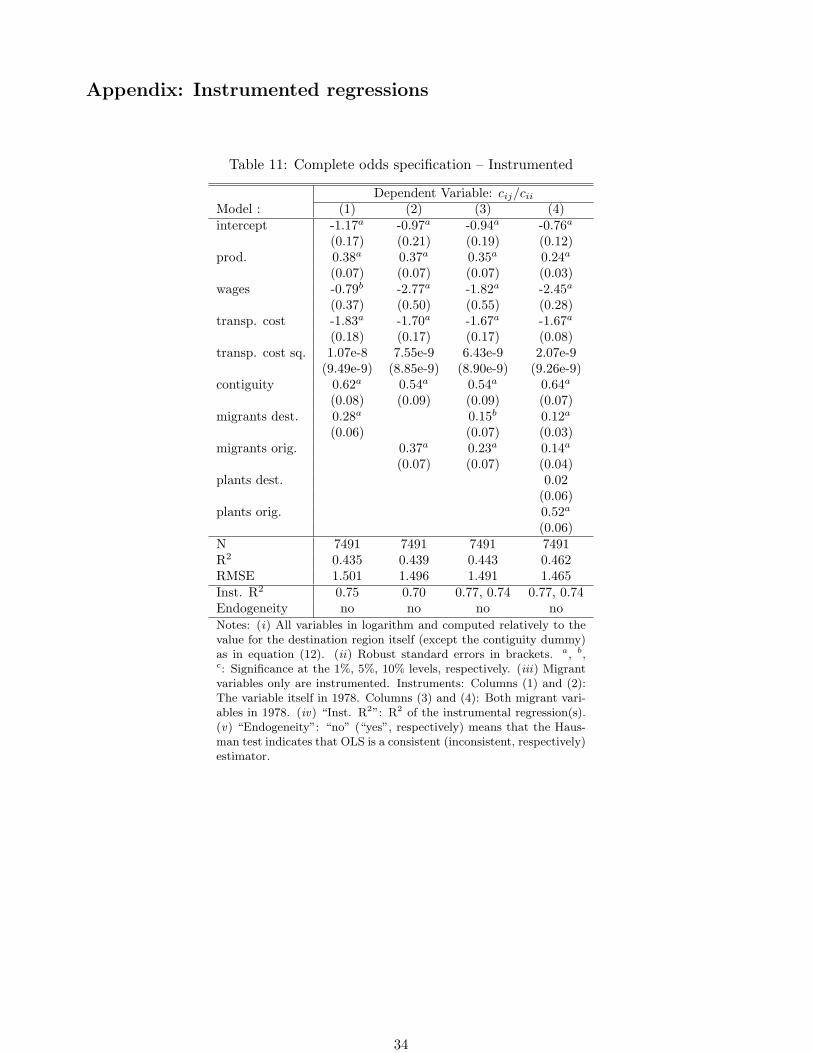
Appendix: Instrumented regressions

Table 11: Complete odds specification – Instrumented

Dependent Variable: cij/ciiModel : (1) (2) (3) (4)intercept -1.17a -0.97a -0.94a -0.76a

(0.17) (0.21) (0.19) (0.12)prod. 0.38a 0.37a 0.35a 0.24a

(0.07) (0.07) (0.07) (0.03)wages -0.79b -2.77a -1.82a -2.45a

(0.37) (0.50) (0.55) (0.28)transp. cost -1.83a -1.70a -1.67a -1.67a

(0.18) (0.17) (0.17) (0.08)transp. cost sq. 1.07e-8 7.55e-9 6.43e-9 2.07e-9

(9.49e-9) (8.85e-9) (8.90e-9) (9.26e-9)contiguity 0.62a 0.54a 0.54a 0.64a

(0.08) (0.09) (0.09) (0.07)migrants dest. 0.28a 0.15b 0.12a

(0.06) (0.07) (0.03)migrants orig. 0.37a 0.23a 0.14a

(0.07) (0.07) (0.04)plants dest. 0.02

(0.06)plants orig. 0.52a

(0.06)N 7491 7491 7491 7491R2 0.435 0.439 0.443 0.462RMSE 1.501 1.496 1.491 1.465Inst. R2 0.75 0.70 0.77, 0.74 0.77, 0.74Endogeneity no no no noNotes: (i) All variables in logarithm and computed relatively to thevalue for the destination region itself (except the contiguity dummy)as in equation (12). (ii) Robust standard errors in brackets. a, b,c: Significance at the 1%, 5%, 10% levels, respectively. (iii) Migrantvariables only are instrumented. Instruments: Columns (1) and (2):The variable itself in 1978. Columns (3) and (4): Both migrant vari-ables in 1978. (iv) “Inst. R2”: R2 of the instrumental regression(s).(v) “Endogeneity”: “no” (“yes”, respectively) means that the Haus-man test indicates that OLS is a consistent (inconsistent, respectively)estimator.

34

Table 12: Friction specification – Instrumented

Dependent Variable: Φij

Model : (1) (2)intercept -0.94a -0.60a

(0.20) (0.20)transport cost -1.49a -1.52a

(0.12) (0.11)transport cost sq. 5.31e-10 -4.53e-9

(9.33e-9) (9.06e-9)contiguity 0.51a 0.63a

(0.09) (0.08)migrants 0.42a 0.27a

(0.05) (0.04)plants 0.76a

(0.09)Inst. R2 0.82 0.82Endogeneity no yesN 3413 3413R2 0.544 0.581RMSE 1.141 1.095Notes: (i) All variables are the logarithm of theproduct of bilateral values computed relativelyto the values for regions themselves (except thecontiguity dummy): See equation (14). (ii) Ro-bust standard errors in brackets. a, b, c: Sig-nificance at the 1%, 5%, 10% levels, respectively.(iii) Migrant variables only are instrumented. In-struments: Columns (1) and (2): The variableitself in 1978. Columns (3) and (4): Both mi-grant variables in 1978. (iv) “Inst. R2”: R2 ofthe instrumental regression(s). (v) “Endogene-ity”: “no” (“yes”, respectively) means that theHausman test indicates that OLS is a consistent(inconsistent, respectively) estimator.

35