the three horsemen of riches: plague, war, and
TRANSCRIPT
The Three Horsemen of Riches:
Plague, War, and Urbanization in Early Modern Europe∗
Nico Voigtländer†, Hans-Joachim Voth‡
First draft: September 2007This draft: June 2012
forthcoming in the Review of Economic Studies
Abstract
How did Europe escape the "Iron Law of Wages?" We construct a simple Malthusian model withtwo sectors and multiple steady states, and use it to explain why European per capita incomes andurbanization rates increased during the period 1350-1700. Productivity growth can only explain a smallfraction of the rise in output per capita. Population dynamics – changes of the birth and death schedules– were far more important determinants of steady states. We show how a major shock to population cantrigger a transition to a new steady state with higher per-capita income. The Black Death was such ashock, raising wages substantially. Because of Engel’s Law, demand for urban products increased, andurban centers grew in size. European cities were unhealthy, and rising urbanization pushed up aggregatedeath rates. This effect was reinforced by diseases spread through war, financed by higher tax revenues.In addition, rising trade also spread diseases. In this way higher wages themselves reduced populationpressure. We show in a calibration exercise that our model can account for the sustained rise in Europeanurbanization as well as permanently higher per capita incomes in 1700, without technological change.Wars contributed importantly to the ’Rise of Europe,’ even if they had negative short-run effects. We thustrace Europe’s precocious rise to economic riches to interactions of the plague shock with the belligerentpolitical environment and the nature of cities.
JEL: E27, N13, N33, O14, O41
Keywords: Malthus to Solow, Long-run Growth, Great Divergence, Epidemics, Demographic Regime
∗We would like to thank the editor, Kjetil Storesletten, and five anonymous referees, as well as Steve Broadberry, Greg Clark,Nick Crafts, Angus Deaton, Matthias Doepke, Oded Galor, Avner Greif, Bob Hall, Nobu Kiyotaki, Ephraim Kleiman, KiminoriMatsuyama, Omer Moav, Joel Mokyr, Rachel Ngai, Ron Lee, Ed Prescott, Diego Puga, Michèle Tertilt, Karine van der Beek,Jaume Ventura, David Weil, and Fabrizio Zilibotti for helpful comments and suggestions. Seminar audiences at Ben Gurion,Brown University, Hebrew University, Humboldt University, the Minnesota Macro Workshop, Northwestern University, PompeuFabra, UC Berkeley, UCLA, Princeton, and Zürich University offered helpful advice. Morgan Kelly shared unpublished results;Mrdjan Mladjan provided outstanding research assistance. Financial support by the Barcelona GSE and the European ResearchCouncil (ERC) is gratefully acknowledged: This paper is produced as part of the project Historical Patterns of Development andUnderdevelopment: Origins and Persistence of the Great Divergence (HI-POD), a Collaborative Project funded by the EuropeanCommission’s Seventh Research Framework Programme, contract number 225342.
†UCLA Anderson School of Management, 110 Westwood Plaza, Los Angeles, CA 90095. Email: [email protected]‡ICREA and Department of Economics, Universitat Pompeu Fabra, c/Ramon Trias Fargas 25-27, E-08005 Barcelona, Spain.
Email: [email protected]
1 Introduction
In 1400, Europe’s potential to overtake the rest of the world seemed limited. The continent was politically
fragmented, torn by military conflict, and dominated by feudal elites. Literacy was low. Other regions, such
as China, appeared more promising. It had a track record of useful inventions, from ocean-going ships togunpowder and advanced clocks (Mokyr, 1990). The country was politically unified, and governed by a
career bureaucracy chosen by competitive exam (Pomeranz, 2000). In 14th century Europe, on the otherhand, few if any of the variables that predict modern-day riches would suggest that its starting position was
favorable.1 By 1700 however, and long before it industrialized, Europe had pulled ahead decisively in termsof per capita income and urbanization – an early divergence preceded the "Great Divergence" that emerged
with the Industrial Revolution (Broadberry and Gupta, 2006; Diamond, 1997).2
This early divergence matters in its own right. It laid the foundations for the European conquest of vast
parts of the globe (Diamond, 1997). It may also have contributed to the even greater differences in percapita incomes that followed. In many unified growth models, an initial rise of per capita income is crucial
for the transition to self-sustaining growth (Galor and Weil, 2000; Hansen and Prescott, 2002). Also, there isgrowing evidence that a country’s development in the more distant past is a powerful predictor of its current
income position (Comin, Easterly, and Gong, 2010). Voigtländer and Voth (2006) develop a model in whichgreater industrialization probabilities are the direct consequence of higher starting incomes. If we are to
understand why Europe achieved the transition from "Malthus to Solow" before other regions of the world,explaining the initial divergence of incomes is crucial.
In a Malthusian economy, the "Iron Law of Wages" should hold – incomes can change temporarily, untilpopulation catches up.3 Nonetheless, many European countries saw marked increases in per capita output.
Maddison (2007) estimates that Western European per capita incomes on average grew by 30% between1500 and 1700. Urbanization rates – often used as a better indicator of per capita output – also rose rapidly.4
In the most successful economies, both incomes and urbanization rates more than doubled. How couldoutput per capita rise substantially in a Malthusian economy?
We develop a simple two-sector model where shocks to population size can lead to permanently higherincomes. Before describing our mechanism, we briefly review the standard Malthusian model in the left
panel of figure 1. Death rates are downward sloping in income, and birth rates are either flat or upwardsloping. This generates a unique steady state (C) that pins down wages and population size. Decreasing
marginal returns to labor set in quickly as population grows because fixed land is an important factor ofproduction. A decline in population can raise wages, moving the economy to the right of C. However, the
1For a recent overview, see Bosworth and Collins (2003), and Sala-i-Martin, Doppelhofer, and Miller (2004).2Western European urbanization rates were more than double those in China (Broadberry and Gupta, 2006; Maddison, 2001).
We discuss the evidence at greater length in section 2 below.3In the words of HG Wells, earlier generations should have always "spent the great gifts of science as rapidly as it got them in
a mere insensate multiplication of the common life" (Wells, 1905). This is the intuition behind Ashraf and Galor (2011), who testfor long-term stagnation of incomes despite variation in soil fertility and agricultural technology.
4Maddison considers urbanization as one of many factors influencing his estimates of GDP. The latest installments of his figurescontain numerous, country-specific adjustments based on detailed research by other scholars.
1
increase in output per capita is only temporary. Birth rates now exceed death rates and population grows,
which in turn will depress wages – the "Iron Law of Wages" holds.5 We modify the standard Malthusianmodel to explain how early modern European incomes could rise permanently. We do so by introducing a
particular mortality regime. In the right-hand panel of figure 1, we show a Malthusian model where deathrates increase with income over some range. We refer to the upward-sloping mortality schedule as the
’Horsemen effect.’ Steady state E0 combines low income per capita with low mortality, while steady stateEH is characterized by higher wages and higher mortality. Point EU is an unstable steady state. Suppose
that the economy starts out in E0. A major positive shock to wages (beyond EU ) will trigger a transition tothe higher-income steady state.
[Insert Figure 1 here]
The Black Death was a shock that raised incomes significantly. It killed between one third and half
of the European population in 1348-50. This raised land-labor ratios, and led to markedly higher wages.In figure 1, such a shock moves the economy beyond point EU . From there, it converges to EH . This is
equivalent to a ’ratchet effect:’ Wage gains after the Black Death became permanent.6
The crucial feature to obtain multiple steady states in figure 1 is an upward-sloping part of the death
schedule. This reflects the historical realities of early modern Europe.7 According to Malthus (1826), factorsreducing population pressure include "vicious customs with respect to women, great cities, unwholesome
manufactures, luxury, pestilence, and war." We focus on three – great cities, pestilence, and war. All of themincreased in importance after the plague because of higher per capita incomes. High wages were partly spent
on manufactured goods, mainly produced in urban areas. Cities in early modern Europe were death-traps,with mortality far exceeding fertility rates. Thus, new demand for manufactures pushed up aggregate death
rates. War and trade reinforced this effect. Between 1500 and 1800, the continent’s great powers werefighting each other on average for nine years out of every ten (Tilly, 1992). This was deadly mainly because
armies on the march often spread epidemics. Wars could be financed more easily when per capita incomeswere high. The difference between income and subsistence increased, leaving more surplus that could be
spent on war. In effect, war was a "luxury good" for princes. In addition, trade grew as people became richer,and it also spread germs.8 In this way, the initial rise in wages after the Black Death was made permanent by
the ’Horsemen effect,’ pushing up mortality rates and producing higher per capita incomes. Thus, Europeexperienced a simultaneous rise in war frequency, in deadly disease outbreaks, and in urbanization. The
5Technological innovation has an affect akin to a drop in population: Wages rise temporarily but eventually converge back tothe unique steady state.
6A large positive shock to technology could theoretically also cause this transition. However, pre-modern rates of productivitygrowth are much too low to trigger convergence to the high-income steady state.
7The theoretical and historical conditions under which the ’Horsemen effect’ led to multiple steady states are discussed in detailin section 2.
8Numerous studies have focused on the interaction between domestic armed conflict and income. Many find that civil warsdecline in frequency after positive growth shocks (Collier and Hoeffler, 1998, 2004; Miguel, Satyanath, and Sergenti, 2004). Incontrast, Grossman (1991) has argued that higher incomes should promote wars ("rapacity" effect), as there is more to fight over.Martin, Mayer, and Thoenig (2008) find that more multilateral trade can lead to more war.
2
Horsemen of the Apocalypse effectively acted as ’Horsemen of Riches.’9
To our knowledge, this study is the first to investigate quantitatively the factors behind Europe’s earlyrise to riches. We do so in a comparative perspective. The great 14th century plague also affected China,
as well as other parts of the world (McNeill, 1977). Why did it not have the same effects there? We arguethat the Chinese demographic regime did not feature multiple steady states. Similar shocks did not lead to
permanently higher death rates for two reasons. Chinese cities were far healthier than European ones. Also,political fragmentation in Europe ensured continuous warfare. China, on the other hand, was politically
unified, except for brief spells of turmoil. There was no link between p.c. income and the frequency of armedconflict. In Western Europe, a unique set of geographical and political starting conditions interacted with
the plague shock to make higher wages sustainable; where these starting conditions were absent, transitionsto higher incomes were much less likely. China can thus be represented by the standard Malthusian model
in the left panel of figure 1, with a unique low-income steady state.We are not the first to argue that higher death rates can raise p.c. income. Young (2005) concludes
that HIV in Africa has a silver lining because it increases the scarcity of labor, boosting the consumption ofsurvivors.10 Clark (2007) highlights the benign effect of higher death rates on p.c. income in the Malthusian
period. Lagerlöf (2003) also examines the interplay of growth and epidemics. He concludes that a declinein the severity of epidemics can foster growth if they stimulate human capital acquisition.11 Brainerd and
Siegler (2003) study the outbreak of "Spanish flu" in the US, and conclude that the states worst-hit in 1918grew markedly faster subsequently. Compared to these papers, we make three contributions. First, we use
the Malthusian model to explain permanently higher wages, not stagnation at a low level. Second, we arethe first to demonstrate how specific European characteristics interacted with a large mortality shock to drive
up incomes over the long run, leading to the ’First Divergence.’ Third, we calibrate our model to show thatit can account for a large part of the ’Rise of Europe’ in the early modern period.
Other related literature includes the unified growth models of Galor and Weil (2000) and Galor andMoav (2002). In both, before fertility limitation sets in and growth becomes rapid, a state variable gradually
evolves over time during the Malthusian regime, making the final escape from stagnation more and morelikely. In Galor and Weil (2000), Jones (2001), and Kremer (1993), the rise in population which in turn
produces more ideas is a key factor; in Galor and Moav (2002), it is the quality of the population.12 Cervellatiand Sunde (2005) argue that the mortality decline from the 19th century onwards was an important element
in the transition to self-sustaining growth, by increasing human capital formation. Hazan (2009) raisesdoubts about the underlying Ben-Porath mechanism. Hansen and Prescott (2002) assume that productivity
9This is the opposite of the negative effect of wars, civil wars, disease, and epidemics on income levels found in many economiestoday (c.f. Murdoch and Sandler, 2002; Hoeffler and Reynal-Querol, 2003). The main reason for this difference is that human capitalis crucial for development today, while it was not in pre-modern times, when decreasing returns to (unskilled) labor in agriculturedominated the production pattern.
10In contrast, Lorentzen, McMillan, and Wacziarg (2008) argue that higher mortality in Africa – including from AIDS – reducesincentives to accumulate capital, and thus reduces growth.
11In a similar vein, Kalemli-Ozcan (2002) argues that declines in mortality were growth-enhancing. Lagerlöf (2010) studiesincome in a Hansen-Prescott type two-sector long-run growth model with war-induced deaths. He shows that the transition to aSolow economy can explain the decline in warfare in the 19th century, i.e., after the period that we focus on.
12Clark (2007) finds some evidence in favor of the Galor-Moav hypothesis, with the rich having more surviving offspring.
3
in the manufacturing sector increases exogenously, until part of the workforce switches out of agriculture;
Desmet and Parente (2009) conclude that market size was key. Strulik and Weisdorf (2008) argue that in aMalthusian regime with a strong preventive check, productivity growth in industry raised the relative cost
of having children.13
Our model emphasizes changes in death rates as a key determinant of output per head. We also show that
technological change can only explain a small fraction of the rising p.c. income in early modern Europe. Oneof the key advantages of our framework is that it can be applied to the cross-section of growth outcomes. In
contrast, the majority of existing unified growth papers implicitly uses the world as their unit of observation.We deliberately limit our attention to the early modern divergence between Europe and China. While models
such as Kremer (1993) and Hansen and Prescott (2002) try to explain the entire transition to self-sustaininggrowth, we simply examine the initial divergence of incomes, long before technological change became
rapid.14
Our paper adds to the literature on the origins of European exceptionalism. Diamond (1997) argued that
a combination of geographical factors with grain and animal endowments in pre-historic times strongly influ-enced which continent did best after 1500. Mokyr (1990) emphasized Europe’s superior record of invention
after 1300. Jones (1981) sees a relatively liberal political environment as key. In the same vein, Acemoglu,Johnson, and Robinson (2005) argue that in Northwestern Europe, Atlantic trade helped to constrain monar-
chical powers, accelerating growth after 1500.15 Our paper emphasizes a combination of geographical andpolitical factors, as well as the peculiar conditions of urban life. These starting conditions interact with the
exogenous shock of the plague in a unique way that could not have occurred in the consolidated imperialstates of the Far East. The large number of European states ensured that higher incomes translated into more
wars. Combined with the filth and overcrowding of European cities, this turned one-off increases in wagesinto permanently higher incomes.
We proceed as follows. The next section provides a detailed discussion of the historical context. Section3 introduces a simple two-sector model that highlights the main mechanism. In section 4, we calibrate our
model and show that it captures the salient features of the ’First Divergence.’ The final section summarizesour findings.
2 Historical Context and Background
In this section we discuss historical evidence for the key elements of the framework presented in figure 1.
A large increase in per capita income can move the economy over the threshold EU so that it converges
13Sharp, Strulik, and Weisdorf (2012) show how falling prices of manufactured goods can lead to fertility decline and thus higherwages in steady state. Vollrath (2011) argues that more labor-intensive agriculture is associated with higher population density andlower per-capita incomes, which can contribute to the First Divergence between Europe and China.
14Galor and Weil (2000) distinguish between a Malthusian, a Post-Malthusian, and a Solow period of growth. We argue in effectthat a period of Malthusian dynamism superseded aeons of Malthusian stagnation, and that doing so prepared the ground for thePost-Malthusian world.
15Their contribution reverses the conclusion of an earlier literature, which had questioned the discoveries’ importance for the’Rise of Europe’ (O’Brien, 1982; Engerman, 1972).
4
to EH – the high income steady state. For this mechanism, an upward-sloping part of the death schedule
is crucial. In the following, we first summarize the impact of the ultimate cause of Europe’s riches in ourmodel – the Black Death’s effect on per capita income. Next, we describe the three factors that cause death
rates to rise with income – urbanization, wars, and trade. In this context, Engel’s Law is important becauseit ensures that manufacturing – and thus urbanization – grows rapidly with income. Finally, we summarize
the evidence for the final outcome, Europe’s precocious rise to riches before 1800 (the "First Divergence").
2.1 The Plague
The plague arrived in Europe from the Crimea in 1347. Tartar troops besieging the Genoese trading outpost
of Caffa passed it on to the defenders. The disease spread with the fleeing Genoese, via Constantinople andSicily to mainland Italy, and finally to the rest of Europe. By December 1350, it had reached the North of
England and the Baltic (McNeill, 1977). Mortality rates amongst those infected varied from 30 to 95%. Bothcities and the countryside suffered. Only a handful of areas in the Low Countries, in Southwest France and
in Eastern Europe were spared the Black Death.16 Aggregate population losses amounted to 15 - 25 mio.,out of a population of roughly 40 mio. The "Great Plague" was followed by a wave of smaller outbreaks.
As shown in the left panel of figure 2, the number of plague epidemics more than quadrupled between the14th and the 17th century, to a peak of 705 in 1630-40. The frequency of outbreaks only declined in the late
17th century.
[Insert Figure 2 here]
Plague was not the only epidemic to strike Europe. There were also outbreaks of smallpox, cholera, and
typhus. Combined with other factors, these epidemics contributed to a downward trend in life expectancy inthe early modern period. The right panel of figure 2 illustrates this for the case of England.
The plague matters in our model because it triggered a large increase in per capita income. The gainsafter 1348 were not fully reversed thereafter. During the "golden age of labor" (Postan, 1972) in England
after 1350, wages approximately doubled (Phelps-Brown and Hopkins, 1981; Clark, 2005). Afterwards, theevidence suggests a decline. Clark (2005) shows that wages fell back from their peak somewhat, but except
for crisis years around the English Civil War, they remained above their pre-plague level.17 The existingwage series therefore reinforce the optimistic GDP figures provided by Maddison (2007), who estimates
that European p.c. income grew by one third between 1500 and 1700.18
16Approximately half of the English clergy died, and in Florence and Venice, death rates have been estimated as high as 60-75%(Ziegler, 1969; Benedictow, 2004).
17The older Phelps-Brown and Hopkins series suggests a stronger decline after 1450. What matters for the predictions of theMalthusian model is per capita output, not wages as such. Accordingly, Broadberry, Campbell, and van Leeuwen (2011) show thatBritish output per head increased by approximately one third in 1350 and stabilized at this high level until the onset of the IndustrialRevolution in the 18th century.
18Not all of Europe did equally well. Allen (2001) found that real wage gains for craftsmen after the Black Death were onlymaintained in Northwestern Europe. In Southern Europe – especially Italy, but also Spain – stagnation and decline after 1500 aremore noticeable. The North-West overtook Southern Europe in terms of urbanization rates and output (Acemoglu et al., 2005).Nonetheless, every European country with the exception of Italy had higher per capita GDP in 1700 than in 1500. Maddison
5
2.2 Elements of the ’Horsemen effect’
In Figure 1, for the existence of multiple equilibria, it is crucial that there is an upward sloping part of the
death schedule – mortality rates have to increase with incomes over some part of the income range. Europe’speculiar mortality pattern was driven by the perils of urban life, and diseases spread by trade and war. We
briefly discuss how each contributed to higher mortality.
City Mortality and Manufacturing
European cities were deadly. Early modern English urban mortality rates were 1.8 times higher than inthe countryside (Clark and Cummins, 2009). A comprehensive survey of rural-urban mortality differences
shows that in Europe before 1800, life expectancy was typically 50 percent higher in the countryside than
in cities (Woods, 2003). In London, 1580-1799, it fluctuated between 27 and 28 years (Landers, 1993), andprovincial towns like York had similar rates of infant mortality (Galley, 1998). At the same time, in England
as a whole, life expectancy was 35-40 years.19
Why did Europeans move to unhealthy cities? First, those who moved were not necessarily the ones
who died – infant mortality was a major contributor to the urban-rural mortality differential. Second, citiesoffered other amenities – a wider range of available goods, and freedom from servitude for those who stayed
long enough. Third, urban wages were generally higher than rural ones. The wage differential reflected theconcentration of manufacturing activities in cities. This was enforced by guilds watching jealously over
their monopoly of producing certain goods. While some manufacturing activity gradually moved to rurallocations from the 16th and 17th century onwards, the vast majority of non-agricultural goods in early modern
Europe was produced in cities and towns (Coleman, 1983).No similar urban mortality penalty existed in China. Chinese infant mortality rates were lower in cities
than in rural areas, and life expectancy was similar or higher.20 Members of Beijing’s elite in the 18th centuryexperienced infant mortality rates that were less than half the rates in France or England.21 On average,
during the period 1644-1899, men born in Beijing had a life expectancy at birth of 31.8 years. In rural Anhui,the corresponding figure was 31 (Lee and Feng, 1999). Other evidence lends indirect support. For example,
life expectancy in Beijing in the 1920s and 1930s was higher than in the countryside.22 Principal reasonsprobably include the transfer of "night soil" (i.e., human excrement) out of the city and onto the surrounding
fields for fertilization, relatively high standards of personal hygiene, and a diet rich in vegetarian food. Sincethe proximity of animals is a major cause of disease, all these factors combined to reduce the urban mortality
assumes that subsistence is equivalent to approximately $400 US-Geary Khamy dollars. Even relatively poor countries like Spainand Portugal had per capita incomes more than twice as high in 1700.
19The only exceptions are two quinquennia when it dropped lower (Wrigley, Davies, Oeppen, and Schofield, 1997). In York,there is not enough data to derive life expectancy. However, infant mortality – a prime determinant of life expectancy – was in thesame range in provincial towns and London.
20The available mortality estimates have been derived from the family trees of clans (Tsui-Jung, 1990), using data from the 15th
to the 19th century.21Woods (2003). The average infant mortality rate in the English cities listed before 1800 is 262; for Beijing, it is 104.22Some recent evidence (Hayami, 2001) on adult mortality questions if Far Eastern cities were indeed healthier than the coun-
tryside, as some scholars have argued (Hanley, 1997; Macfarlane, 1997). There is no discussion about the cities being markedlyless healthy.
6
burden in the Far East.
Relatively high urban mortality in Europe also reflected the way in which cities were built. Becausewarfare was common, European cities were typically surrounded by fortifications. These limited city growth
(De Vries, 1976). In China, the defensive function of city walls declined after the country’s unification;houses and markets spread outside the city walls. This reduced overcrowding and kept mortality rates
relatively low.
Engel’s Law
Consumers grown rich(er) after the Black Death spent relatively less on food, and more on manufacturing
goods: Consumption patterns in medieval England suggest that Engel’s Law held. Dyer (1988) documentshow the share of income spent on food declined with social status. Peasants spent a high proportion; clerical
households earning £20, half of their income; earls earning thousands of pounds sterling, less than a quarter.Over time, following the Black Death, the pattern is also clear. Spending by peasants on dwellings, clothing,
cooking utensils, ceramics, and furniture all increased (as reflected in probate inventories).23 For England inthe early modern period, the income elasticity of food expenditure was 0.76 (Horrell, 1996). This is similar
to estimates for present-day India (0.7, as derived in Subramanian and Deaton, 1996). In combination, thereis ample evidence – both in the cross-section, and over time – that Engel’s law applied after 1350.
The Impact of War
War matters for our model because it pushed up aggregate death rates, raising land-labor ratios. We also ar-gue that it had relatively limited negative direct effects on output, acting more as the early modern equivalent
of a "neutron bomb."Battlefield casualties were generally low, compared to aggregate death rates.24 Armies were generally
too small for military deaths to influence aggregate mortality rates substantially.25 Instead, early modernarmies killed by exposing isolated communities to new germs. In one famous example, a single army of
6,000 men, dispatched from La Rochelle (France) to deal with the Mantuan Succession in Northern Italy,spread plague that may have killed up to one million people (Landers, 2003). As late as the Napoleonic
wars, typhus, smallpox and other diseases spread by armies marauding across Europe proved far deadlierthan guns and swords.
Aggregate civilian population losses in wartime could be heavy. The Holy Roman Empire lost 5-6 mio.out of 15 mio. inhabitants during the Thirty Years War; 20% of the French population died in the late 16th
century as a result of civil war. The figures for early 17th century Germany and 16th century France imply
23Dyer (1988) also notes that the quality of goods improved: "Pewter tableware and metal ewers replaced some wood and potteryvessels for more substantial peasants, and ceramic cisterns supplanted wooden casks. Potters began to supply cups, which had allpreviously been made of wood... The dice, cards, chessmen, footballs, musical instruments and ’nine-men’s morris’ boards showthat resources could be spared..."
24Data on deaths caused by military operations in the early modern period are sketchy. Landers (2003) offers an overview ofbattlefield deaths. Lindegren (2000) finds that military deaths only raised Sweden’s aggregate death rates by 2-3/1000 in mostdecades between 1620 and 1719, a rise of no more than 5%. Castilian military deaths were 1.3/1000, equivalent to 10 percent ofadult male deaths but no more than 3-4% of overall deaths.
25Since infant mortality was high, by the time men could join the army, many male children had died already. This makes it lesslikely for military deaths to matter in the aggregate.
7
that aggregate mortality rates rose by 50 to 100%, and that these rates were sustained for decades. For
the early and mid-nineteenth century, we have additional data on the indirect, country-wide rise in mortalityfrom warfare. During the Swedish-Russian war of 1808-09, mortality rates in all of Sweden doubled, almost
exclusively through disease. In isolated islands, the presence of Russian troops – without any fighting – ledto a tripling of death rates (Landers, 2003).
Warfare became increasingly expensive during the early modern period (Landers, 2003; Tilly, 1992).The "military revolution" brought professional, drilled troops, Italian-style fortifications, ships, muskets,
and cannons. To make war, princes had to draw on liquid funds. After the plague, incomes per capita werehigher; there was more surplus above subsistence that could be expropriated. As a result of the so-called
’commercial revolution’ of the late Middle Ages, the economy had already become more urban, monetizedand commercialized (Lopez, 2008). Surpluses could be taxed more easily, providing the means for fighting
more, and fighting longer. In figure 3, we show the tight link between urbanization rates and tax revenue percapita (as a percentage of the average wage), between 1500 and 1800 (the correlation coefficient is 0.87).26
China in the early modern period saw markedly less warfare than Europe (Pomeranz, 2000). Even on agenerous definition, wars and armed uprisings only occurred in one year out of five, no more than a quarter
of the European frequency.27 Why did Europe see much more inter-state conflict than other parts of theglobe? Tilly (1992) emphasizes the fragmented nature of the European political system in the late medieval
period. In addition, after the Reformation, religious strife contributed to frequent warfare (Jones, 1981).Compared to that, politically unified states like China had many fewer "flash points" leading to military
conflict.
[Insert Figure 3 here]
Not only were wars fewer in China after 1400. They also caused fewer epidemics. Europe is geo-graphically subdivided by rugged mountain ranges and large rivers, with considerable variation in climatic
conditions. China’s main population areas were more homogenous in geographical terms than Europe’s.The history of epidemics in China suggests that by 1000 AD, disease pools had become largely integrated
(McNeill, 1977). Hence, troop movements produced less of a surge in Chinese death rates than in Europe.28
Pre-modern wars were deadly, but they destroyed little capital. Military technology was too primitive
to cause widespread destruction. De Vries (1976) concluded that "it is hard to prove that military action
checked the growth of the European economy’s aggregate output." Malthus himself noted the remarkableability of early modern economies to bounce back from war-induced destruction.29
26We normalize by the wage since this shows that the growth in tax revenue does not simply reflect higher incomes. Instead, itshows that tax revenues grew disproportionately as urbanization increased.
27Counting battles (instead of wars) reinforces this result – there were 1,071 major battles (not peasant revolts, etc.) in Europebetween 1400 and 1800. The corresponding figure for China is 23 (Jaques, 2007).
28We are indebted to David Weil for this point. Weil (2004) shows the marked similarity of agricultural conditions in large partsof modern-day China.
29"The fertile province of Flanders, which has been so often the seat of the most destructive wars, after a respite of a few years,has appeared always as fruitful and as populous as ever. Even the Palatinate lifted up its head again after the execrable ravages ofLouis the Fourteenth" (Malthus, 1798).
8
Several factors kept economic losses small. Pay constituted the single largest expenditure item in war,
and was largely recycled in the local economy. Destruction of capital mattered less where it could be rebuiltquickly. Wooden houses were easy to reconstruct.30 Where fields went untended, agricultural productivity
rose – fallowing increased land fertility. Farm animals have high natural fertility rates, and losses of livestockcan be made up quickly. Finally, war-induced mortality, where it resulted from poor nutrition, was probably
concentrated amongst the more vulnerable groups – the young and the elderly (Tallett, 1992). Thus, waralso reduced the dependency burden.
In our baseline modeling, we will assume that war shifted the mortality schedule, but that it did not affectproductivity. We also examine the effects of negative productivity from warfare in appendix A.8. While this
changes the short-term dynamics, we show that our long-run results are unaffected.
Trade
Trade in early modern Europe frequently spread disease. The Black Death’s advance in the 14th centuryfollowed trade routes (Herlihy, 1997). The last outbreak in Europe is also linked to long-distance trade. A
plague ship from the Levant docked in Marseille in 1720, infecting the local population. It is estimated that50,000 out of 90,000 inhabitants died in the subsequent outbreak (Mullett, 1936). As transport infrastruc-
tures improved, trade increased massively between the medieval period and the eighteenth century. Canalsand better coastal shipping made it possible to trade bulky goods. Since trade increases with per capita
incomes, the positive effect of the Black Death on wages created knock-on effects. These raised mortalityrates yet further. Finally, there were interaction effects between the channels we have highlighted. The
effectiveness of quarantine measures, for example, often declined when wars disrupted administrative pro-cedure (Slack, 1981). All these factors in combination ensured that, after the Black Death, European death
rates increased, and stayed high, in a way that is unlikely to have occurred in other parts of the world.
2.3 European Economic Performance and the First Divergence between Europe and China
After 1350, European per capita incomes surged ahead of those in other parts of the world, most notably
China – a ’First Divergence’ occurred long before the Industrial Revolution. In addition to the real wageevidence discussed above, this conclusion is supported by urbanization rates. These have been widely used
as an indicator of economic development (e.g., Acemoglu et al., 2005). Urbanization rates support theview that Europe’s economy performed well during the early modern period. By this measure, Europe
overtook China at some point between 1300 and 1500, extending its lead thereafter. Figure 4 summarizesthe evidence. We use data from Bairoch, Batou, and Chèvre (1988) and De Vries to construct a consistent
series for the period 1000 - 1800.31 There is a sharp acceleration of urban growth after the 1350, with thepercentage of the population living in cities (with more than 10,000 inhabitants) rising from about 3 to 9
30After the Turkish siege of Vienna in 1683, the Venetian ambassador marveled at the fact that "the suburbs...as well as theneighbouring countryside...have been completely rebuilt in a short space of time" (Tallett, 1992).
31De Vries (1984) uses a cut-off of 10,000 inhabitants to define cities, and shows that the proportion of Europeans living in urbancenters grew from 5.6 to 9.2 percent between 1500 and 1700. His figures only start in 1500. We extend this series using Bairochet al. (1988). Appendix A.1 provides a detailed description of our method.
9
percent during the three centuries after the Black Death.32
[Insert Figure 4 here]
Other regions of the world did not experience similar, sustained growth during this period. The contrastin economic performance with China is particularly instructive. Adam Smith had no doubt that the "real
recompense of labour is higher in Europe than in China" (Smith, 1776). Malthus and many other scholarsagreed (Elvin, 1973; Jones, 1981). While the most pessimistic interpretations of Chinese economic perfor-
mance have been challenged by the "California School," there is convincing evidence that European outputper capita by the end of the early modern period was markedly higher.33
For example, the proportion of the Chinese population living in cities reached 3 percent in the mid-T’angdynasty (762), 3.1 percent in the mid-Sung dynasty (1120), and probably stagnated at the 3-4 percent level
thereafter until the 19th century (Maddison, 2001; see the dashed line in figure 4). Eastern Europe had lowrates of urbanization overall, and it only saw minor increases after 1500. De Vries (1984) shows gains of
1.5% for the period 1500-1700. Similarly, the Middle East – while highly urbanized on some measures –stagnated in terms of urbanization between 1100 and 1800 (Bosker, Buringh, and van Zanden, 2008).
Wage data point in the same direction. Expressed as units of grain or rice, English wages were markedlyhigher throughout the early modern period than Chinese ones: Chinese grain-equivalent wages were 87% of
English ones in 1550-1649, falling to 38% in 1750-1849 Broadberry and Gupta (2006). Expressed in unitsof silver, the differences are even more striking. Allen (2009) finds that Chinese hired farm laborers earned
only one third of the wage of their English peers.34
By the late 18th century, English agriculture released labor on a massive scale to the cities. In contrast,
Chinese agriculture did not release labor; it hoarded it. Allen (2009) shows that output per year and headprobably fell by 40% between 1620 and 1820 in Chinese agriculture, as average farm size declined. He
concludes that "real wage comparisons push the start of the ’Great Divergence’ back from the nineteenthcentury to the seventeenth." This is the view that underlies our interpretation – Chinese output per capita,
while not necessarily below the European norm at the beginning of the early modern period, stagnated orfell for most of it. In contrast, wages and incomes grew in Europe.
Chinese vs. European demography
Our model explains the first divergence between Europe and China as a result of demographic differences
and interactions with the political environment. Demography differed substantially between the two re-gions. Chinese demographic growth was much more rapid than in Europe: Population in China grew by
170% between 1500 and 1820; in Europe, the corresponding figure is 38%.35 A long tradition of scholar-32Prior to the Black Death, Medieval Europe did not experience a similar upward trend in urban population shares. Urban growth
per century was about three times faster in 1300-1700 than in 1000-1300.33Pomeranz (2000) compares England with the Yangtze delta, China’s most productive area. He concludes that Chinese peasants’
incomes were similar or higher in terms of calories than those of English farmers. His work receives support from Li (1998), whopresents optimistic conclusions about grain production in Jiangnan.
34At the same time, peasant farmers who tilled their own soil may have done better than their English contemporaries in the 17th
century. Thereafter, English earnings overtook Chinese ones (Allen, 2009).35Maddison (2007); Lee and Feng (1999) also show Chinese population grew faster than the world on average.
10
ship emphasized differences in fertility – Europeans practiced fertility limitation, by postponing marriage
and having a high percentage of women that never married. In China, marriage occurred early and wasuniversal.36
3 The Model
In this section, we describe the two-sector Malthusian model summarized in the introduction (see figure 1).
The economy is composed of N identical individuals who work, consume, and procreate. NA individualswork in agriculture (A) and live in the countryside, while NM agents live in cities producing manufacturing
output (M ). Production takes place under perfect competition. For simplicity, we assume that there is nophysical capital or storage; wages are the only source of income. Labor mobility ensures that rural and urban
wages equalize. Peasants own their land and pass it on to their children; when peasants migrate to cities,their land is distributed equally among the remaining rural population.37 Agricultural output is produced
using labor and a fixed land area. This implies decreasing returns in food production. Manufacturing useslabor only and is subject to constant returns to scale. Preferences over the two goods are non-homothetic
and reflect Engel’s law: The share of manufacturing expenditures (and thus the urbanization rate NM/N )grows with p.c. income. Technology parameters in both sectors, AA and AM , are fixed throughout the main
part of our analysis. We introduce exogenous technological change below in section 4.3, where we analyzeits contribution to the ’Rise of Europe.’
A proportional tax τ on manufactured goods provides the funds for warfare – the higher tax revenues,the larger the proportion of population affected. Wars spread diseases. As the scale of warfare rises, more
distant, less immune populations are affected; aggregate mortality surges. However, this rise only continues
until the entire population has been affected. Beyond this point, additional warfare does not raise mortality.
3.1 Consumption
Each individual supplies one unit of labor inelastically in every period. There is no investment – all income
is spent on agricultural goods (cA) and manufactured goods (cM ). Agents choose their workplace in orderto maximize income. When migration is unconstrained, this equalizes urban and rural wages: wA = wM =
36Recent research instead argues that fertility rates were not too different overall, with infanticide and low fertility within marriagereducing Chinese birth rates (Lee and Feng, 1999). With comparable fertility rates but much faster population growth in China,mortality rates overall there must have been lower than in Europe. Since income per capita was below the European level, fertilityrates controlling for income were markedly higher in China, while mortality was lower. In other words, given how rich Europeanswere, they should have lived longer and had more children if Europe and China had shared a demographic regime. Instead,Europeans died early and had few children despite their riches. This paper explains why this does not constitute a paradox, byarguing that specific European factors driving up mortality rates pushed up per capita incomes.
37Migration in the opposite direction is irrelevant in our model. Our setup can be interpreted as a reduced form of a more generalmodel with a continuum of representative infinitely lived dynasties. Fertility and mortality depend on consumption, and we assumefor simplicity that parents ignore (or do not internalize) the utility of their children as well as the link between demography andconsumption. Thus, similar to Blanchard (1985), individuals face a given probability of death in each period, and a given fertilitythat is realized during the last period of life. Upon death, children inherit the property rights of land in equal shares. Under theseassumptions, the dynamic problem reduces to a sequence of static problems that we model below.
11
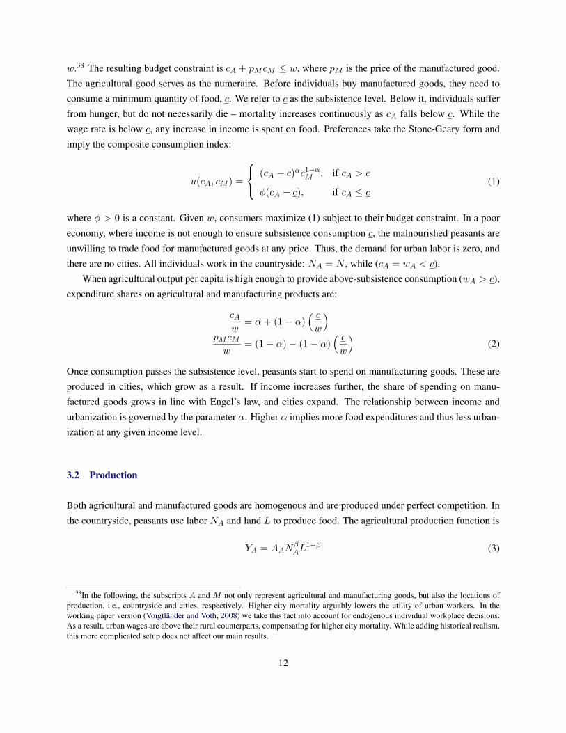
w.38 The resulting budget constraint is cA + pMcM ≤ w, where pM is the price of the manufactured good.
The agricultural good serves as the numeraire. Before individuals buy manufactured goods, they need toconsume a minimum quantity of food, c. We refer to c as the subsistence level. Below it, individuals suffer
from hunger, but do not necessarily die – mortality increases continuously as cA falls below c. While thewage rate is below c, any increase in income is spent on food. Preferences take the Stone-Geary form and
imply the composite consumption index:
u(cA, cM ) =
(cA − c)αc1−αM , if cA > c
ϕ(cA − c), if cA ≤ c(1)
where ϕ > 0 is a constant. Given w, consumers maximize (1) subject to their budget constraint. In a poor
economy, where income is not enough to ensure subsistence consumption c, the malnourished peasants areunwilling to trade food for manufactured goods at any price. Thus, the demand for urban labor is zero, and
there are no cities. All individuals work in the countryside: NA = N , while (cA = wA < c).When agricultural output per capita is high enough to provide above-subsistence consumption (wA > c),
expenditure shares on agricultural and manufacturing products are:
cAw
= α+ (1− α)( c
w
)pMcMw
= (1− α)− (1− α)( c
w
)(2)
Once consumption passes the subsistence level, peasants start to spend on manufacturing goods. These areproduced in cities, which grow as a result. If income increases further, the share of spending on manu-
factured goods grows in line with Engel’s law, and cities expand. The relationship between income andurbanization is governed by the parameter α. Higher α implies more food expenditures and thus less urban-
ization at any given income level.
3.2 Production
Both agricultural and manufactured goods are homogenous and are produced under perfect competition. In
the countryside, peasants use labor NA and land L to produce food. The agricultural production function is
YA = AANβAL
1−β (3)
38In the following, the subscripts A and M not only represent agricultural and manufacturing goods, but also the locations ofproduction, i.e., countryside and cities, respectively. Higher city mortality arguably lowers the utility of urban workers. In theworking paper version (Voigtländer and Voth, 2008) we take this fact into account for endogenous individual workplace decisions.As a result, urban wages are above their rural counterparts, compensating for higher city mortality. While adding historical realism,this more complicated setup does not affect our main results.
12
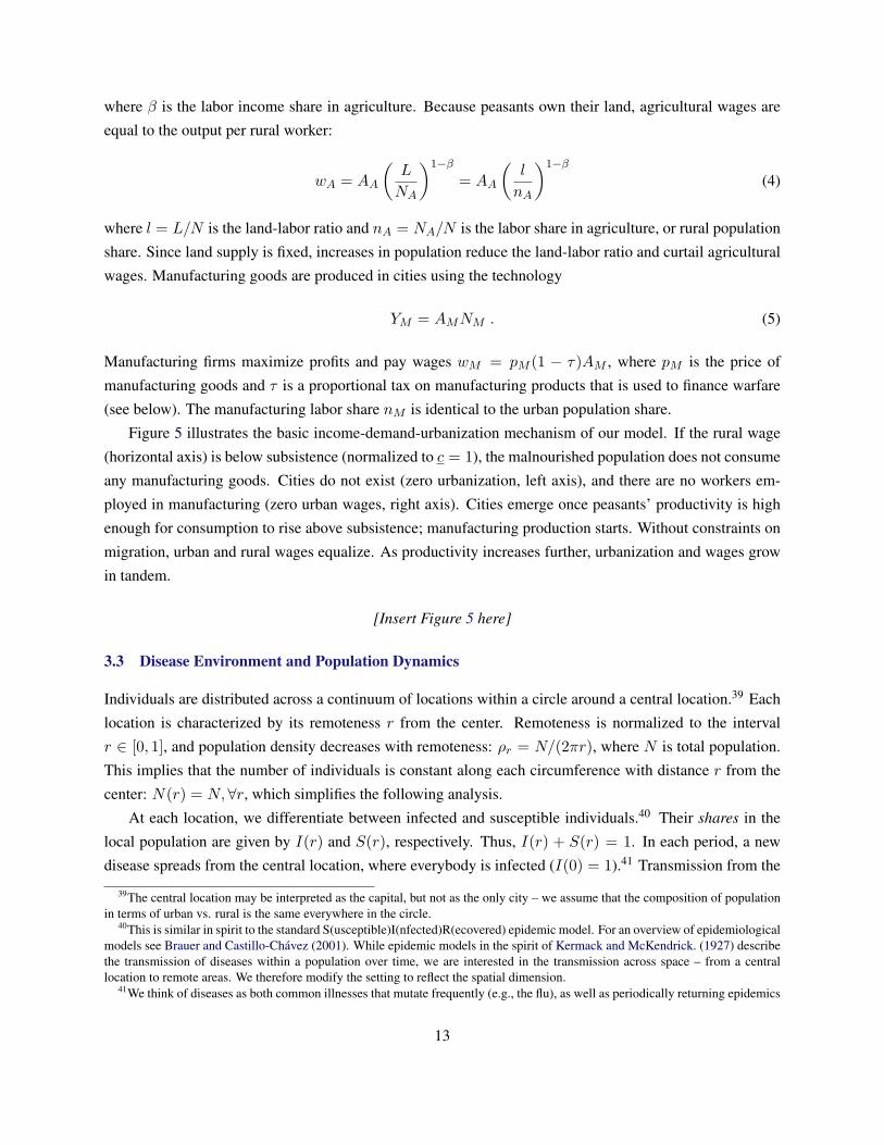
where β is the labor income share in agriculture. Because peasants own their land, agricultural wages are
equal to the output per rural worker:
wA = AA
(L
NA
)1−β
= AA
(l
nA
)1−β
(4)
where l = L/N is the land-labor ratio and nA = NA/N is the labor share in agriculture, or rural population
share. Since land supply is fixed, increases in population reduce the land-labor ratio and curtail agriculturalwages. Manufacturing goods are produced in cities using the technology
YM = AMNM . (5)
Manufacturing firms maximize profits and pay wages wM = pM (1 − τ)AM , where pM is the price ofmanufacturing goods and τ is a proportional tax on manufacturing products that is used to finance warfare
(see below). The manufacturing labor share nM is identical to the urban population share.Figure 5 illustrates the basic income-demand-urbanization mechanism of our model. If the rural wage
(horizontal axis) is below subsistence (normalized to c = 1), the malnourished population does not consumeany manufacturing goods. Cities do not exist (zero urbanization, left axis), and there are no workers em-
ployed in manufacturing (zero urban wages, right axis). Cities emerge once peasants’ productivity is highenough for consumption to rise above subsistence; manufacturing production starts. Without constraints on
migration, urban and rural wages equalize. As productivity increases further, urbanization and wages growin tandem.
[Insert Figure 5 here]
3.3 Disease Environment and Population Dynamics
Individuals are distributed across a continuum of locations within a circle around a central location.39 Eachlocation is characterized by its remoteness r from the center. Remoteness is normalized to the interval
r ∈ [0, 1], and population density decreases with remoteness: ρr = N/(2πr), where N is total population.This implies that the number of individuals is constant along each circumference with distance r from the
center: N(r) = N, ∀r, which simplifies the following analysis.At each location, we differentiate between infected and susceptible individuals.40 Their shares in the
local population are given by I(r) and S(r), respectively. Thus, I(r) + S(r) = 1. In each period, a newdisease spreads from the central location, where everybody is infected (I(0) = 1).41 Transmission from the
39The central location may be interpreted as the capital, but not as the only city – we assume that the composition of populationin terms of urban vs. rural is the same everywhere in the circle.
40This is similar in spirit to the standard S(usceptible)I(nfected)R(ecovered) epidemic model. For an overview of epidemiologicalmodels see Brauer and Castillo-Chávez (2001). While epidemic models in the spirit of Kermack and McKendrick. (1927) describethe transmission of diseases within a population over time, we are interested in the transmission across space – from a centrallocation to remote areas. We therefore modify the setting to reflect the spatial dimension.
41We think of diseases as both common illnesses that mutate frequently (e.g., the flu), as well as periodically returning epidemics
13
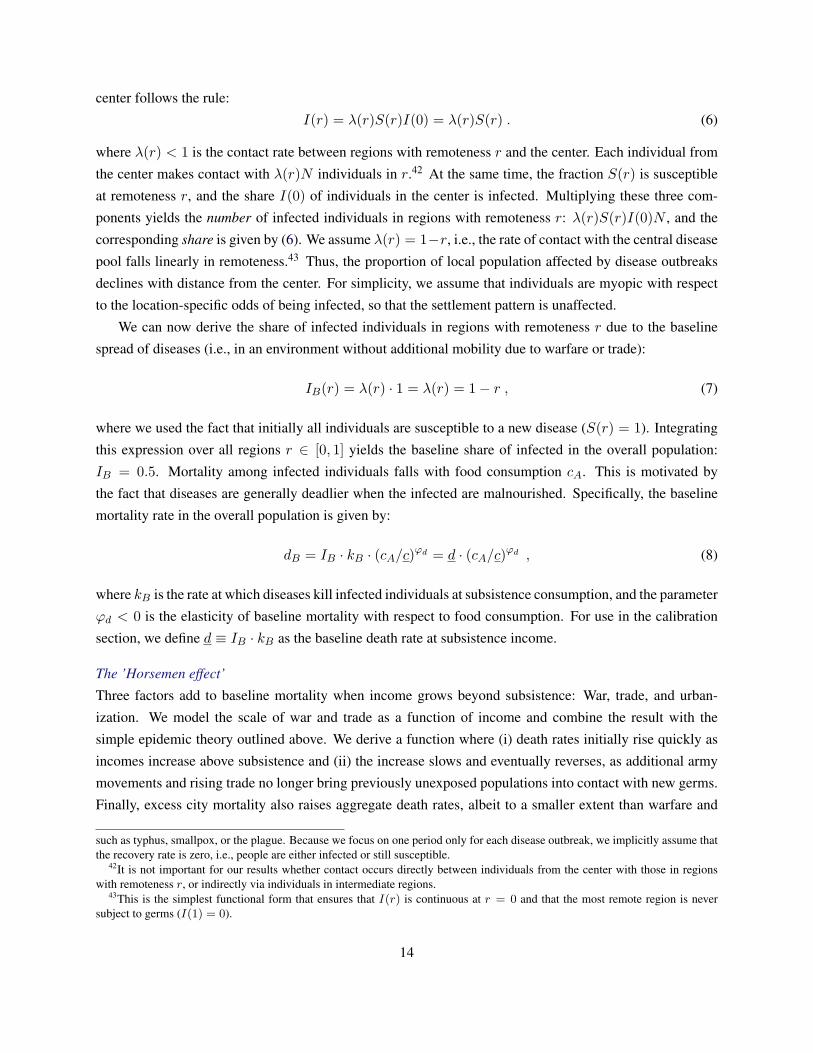
center follows the rule:
I(r) = λ(r)S(r)I(0) = λ(r)S(r) . (6)
where λ(r) < 1 is the contact rate between regions with remoteness r and the center. Each individual fromthe center makes contact with λ(r)N individuals in r.42 At the same time, the fraction S(r) is susceptible
at remoteness r, and the share I(0) of individuals in the center is infected. Multiplying these three com-ponents yields the number of infected individuals in regions with remoteness r: λ(r)S(r)I(0)N , and the
corresponding share is given by (6). We assume λ(r) = 1−r, i.e., the rate of contact with the central diseasepool falls linearly in remoteness.43 Thus, the proportion of local population affected by disease outbreaks
declines with distance from the center. For simplicity, we assume that individuals are myopic with respectto the location-specific odds of being infected, so that the settlement pattern is unaffected.
We can now derive the share of infected individuals in regions with remoteness r due to the baselinespread of diseases (i.e., in an environment without additional mobility due to warfare or trade):
IB(r) = λ(r) · 1 = λ(r) = 1− r , (7)
where we used the fact that initially all individuals are susceptible to a new disease (S(r) = 1). Integratingthis expression over all regions r ∈ [0, 1] yields the baseline share of infected in the overall population:
IB = 0.5. Mortality among infected individuals falls with food consumption cA. This is motivated bythe fact that diseases are generally deadlier when the infected are malnourished. Specifically, the baseline
mortality rate in the overall population is given by:
dB = IB · kB · (cA/c)φd = d · (cA/c)φd , (8)
where kB is the rate at which diseases kill infected individuals at subsistence consumption, and the parameterφd < 0 is the elasticity of baseline mortality with respect to food consumption. For use in the calibration
section, we define d ≡ IB · kB as the baseline death rate at subsistence income.
The ’Horsemen effect’
Three factors add to baseline mortality when income grows beyond subsistence: War, trade, and urban-
ization. We model the scale of war and trade as a function of income and combine the result with thesimple epidemic theory outlined above. We derive a function where (i) death rates initially rise quickly as
incomes increase above subsistence and (ii) the increase slows and eventually reverses, as additional armymovements and rising trade no longer bring previously unexposed populations into contact with new germs.
Finally, excess city mortality also raises aggregate death rates, albeit to a smaller extent than warfare and
such as typhus, smallpox, or the plague. Because we focus on one period only for each disease outbreak, we implicitly assume thatthe recovery rate is zero, i.e., people are either infected or still susceptible.
42It is not important for our results whether contact occurs directly between individuals from the center with those in regionswith remoteness r, or indirectly via individuals in intermediate regions.
43This is the simplest functional form that ensures that I(r) is continuous at r = 0 and that the most remote region is neversubject to germs (I(1) = 0).
14
trade.
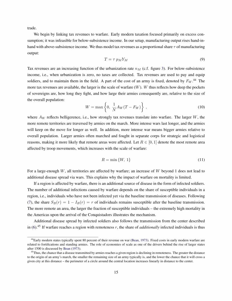
We begin by linking tax revenues to warfare. Early modern taxation focused primarily on excess con-sumption; it was infeasible for below-subsistence income. In our setup, manufacturing output rises hand-in-
hand with above-subsistence income. We thus model tax revenues as a proportional share τ of manufacturingoutput:
T = τ pMYM (9)
Tax revenues are an increasing function of the urbanization rate nM (c.f. figure 3). For below-subsistenceincome, i.e., when urbanization is zero, no taxes are collected. Tax revenues are used to pay and equip
soldiers, and to maintain them in the field. A part of the cost of an army is fixed, denoted by FW .44 Themore tax revenues are available, the larger is the scale of warfare (W ). W thus reflects how deep the pockets
of sovereigns are, how long they fight, and how large their armies consequently are, relative to the size ofthe overall population:
W = max
{0,
1
NAW (T − FW )
}, (10)
where AW reflects belligerence, i.e., how strongly tax revenues translate into warfare. The larger W , themore remote territories are traversed by armies on the march. More intense wars last longer, and the armies
will keep on the move for longer as well. In addition, more intense war means bigger armies relative tooverall population. Larger armies often marched and fought in separate corps for strategic and logistical
reasons, making it more likely that remote areas were affected. Let R ∈ [0, 1] denote the most remote areaaffected by troop movements, which increases with the scale of warfare:
R = min {W, 1} (11)
For a large-enough W , all territories are affected by warfare; an increase of W beyond 1 does not lead to
additional disease spread via wars. This explains why the impact of warfare on mortality is limited.If a region is affected by warfare, there is an additional source of disease in the form of infected soldiers.
The number of additional infections caused by warfare depends on the share of susceptible individuals in aregion, i.e., individuals who have not been infected yet via the baseline transmission of diseases. Following
(7), the share SB(r) = 1 − IB(r) = r of individuals remains susceptible after the baseline transmission.The more remote an area, the larger the fraction of susceptible individuals – the extremely high mortality in
the Americas upon the arrival of the Conquistadors illustrates the mechanism.Additional disease spread by infected soldiers also follows the transmission from the center described
in (6).45 If warfare reaches a region with remoteness r, the share of additionally infected individuals is thus
44Early modern states typically spent 80 percent of their revenue on war (Bean, 1973). Fixed costs in early modern warfare arerelated to fortifications and standing armies. The role of economies of scale as one of the drivers behind the rise of larger statesafter 1500 is discussed by Bean (1973).
45Thus, the chance that a disease transmitted by armies reaches a given region is declining in remoteness. The greater the distanceto the origin of an army’s march, the smaller the remaining size of an army typically is, and the lower the chance that it will cross agiven city at this distance – the perimeter of a circle around the central location increases linearly in distance to the center.
15
given by:
IW (r) = λ(r)SB(r)I(0) = λ(r)r = (1− r)r . (12)
Warfare reaches all regions with remoteness r ≤ R. In even more remote regions, there are no additionalinfections due to warfare. Therefore, we obtain:
IW (r) =
(1− r)r, if r ≤ R
0, if r > R(13)
Next, we derive the average economy-wide share of individuals that are infected due to warfare. Integrating
over r ∈ [0, 1] yields:
IW (R) =
∫ 1
0IW (r)dr =
∫ R
0(1− r)rdr =
1
2R2 − 1
3R3 . (14)
We show below that R is an increasing function of the urbanization rate nM , so as to obtain IW (nM ).Following the same setup as for baseline mortality in (8), the war-related additional death rate is thus given
bydW = IW (nM ) · kB · (cA/c)φd = hW (nM ) · d · (cA/c)φd , (15)
where hW (nM ) ≡ IW (nM )/IB is the war-related ’Horsemen effect,’ i.e., the percentage increase in infec-
tions (and thus aggregate mortality) due to warfare.Trade spreads disease in a similar fashion as warfare. Trade increases with manufacturing output, and
the fixed cost in (10) can be interpreted as expenses for trade infrastructure. The effect of trade on deathrates can thus be modeled along the same lines as warfare, such that hW (nM ) represents both war- and
trade-related disease spread.Finally, higher urbanization raises aggregate death rates because city mortality is above the baseline
level. We represent this fact by a higher death rate of infected individuals in cities, kM > kB . With theproportion nM of individuals dwelling in cities, the corresponding additional impact on aggregate death
rates is given by hM (nM ) = (kM/kB − 1) · nM .46 This is the urbanization-related ’Horsemen effect.’Aggregate death rates are given by baseline mortality, augmented by war, trade, and urbanization:
d = [1 + hW (nM ) + hM (nM )] · d · (cA/c)φd = [1 + h(nM )] · d · (cA/c)φd , (16)
where h(nM ) denotes the aggregate ’Horsemen effect.’ When the Horsemen ride, increasing income has anambiguous effect on mortality. On the one hand, the Horsemen raise background mortality. On the other
hand, greater food consumption translates into lower baseline death rates in (8). The aggregate impact ofincome on mortality depends on the model parameters. Our calibration in section 4.1 demonstrates that
46More specifically, urban death rates are given by dM = IB · kM · (cA/c)φd = (kM/kB) · d · (cA/c)φd . We thus assumethat the share of infected is the same in urban and rural areas, while the deadliness of diseases is different. Alternatively, we couldassume that the rate of infections is larger in cities, which would yield identical results.
16
death rates increase in income – and thus in urbanization – over some range, following an S-shaped pattern
as shown in the right-hand panel of Figure 1.
Population Dynamics
Birth rates depend on nutrition, measured by food consumption cA. Individuals procreate at the rate
b = b · (cA/c)φb (17)
where φb > 0 is the elasticity of the birth rate with respect to nutrition, and b represents the birth rate at
subsistence consumption.Population growth equals the difference between the average birth and death rate, γN = b − d, where
the latter can include the ’Horsemen effect.’ The law of motion for aggregate population N is thus
N ′ = (1 + b− d)N , (18)
where N ′ denotes next period’s population. Births and deaths occur at the end of a period, such that allindividuals N enter the workforce in the current period.
3.4 Steady States
A steady state in our model is characterized by constant output per worker, labor shares, wages, prices,and consumption expenditure shares. We begin by analyzing the economy without technological progress;
in this case, population is also constant in steady state, so that (18) implies b = d.47 Equating (16) and(17) yields an expression that implicitly defines steady state income and illustrates the intuition behind the
’Horsemen effect.’c∗Ac
=
((1 + h∗) · d
b
) 1φb−φd
, (19)
where the asterisk denotes steady state levels. Because φb − φd > 0, an increase in death rates due to the’Horsemen effect’ h∗ raises per capita food consumption (and thus income) in steady state. Multiple steady
states can arise if the function h(nM ) increases in urbanization (and thus income) over some range. Thesteady state level of variables depends on the position of the birth and death schedules. Figure 1 visualizes
the shape of the schedules, depicting the S-shaped pattern of aggregate mortality as implied by (16).48
Points E0 and EH in figure 1 are stable steady states with endogenous population size. During the
transition to steady state, population dynamics influence the land-labor ratio and thus output per worker.Consequently, wages, expenditure shares, prices, and labor shares all change during the transition. In the
following, we analyze these dynamics.
47In the presence of ongoing technological progress, population grows at a constant rate (see section 4.3).48Figure 1 refers to a simple one-sector setup. Because food consumption cA is proportional to wages (see equation (2)), we can
use the same figure to illustrate the intuition in our two-sector model.
17
3.5 Solving the Dynamic Model
The Economy with Below-Subsistence Consumption
To check if agricultural productivity (determined by AA and the land-labor ratio) is sufficient to ensure
above-subsistence consumption, we construct the indicator w, assuming that all individuals work in agricul-ture. Equation (3) with NA = N gives the corresponding per-capita income:
w ≡ YA(N)
N= AA
(L
N
)1−β
(20)
If w ≤ c, all individuals work in agriculture and spend their entire income on food. Since there is nodemand for manufacturing goods (cM = 0), the manufacturing price is zero. This implies zero urban wages
and zero city population (wM = 0 and nM = 0). In addition, wA = cA = w, which can be used in (16)and (17) to derive population growth.49 These equations characterize the economy with below-subsistence
consumption. In principle, our model can have a steady state with below-subsistence consumption, such thatthe economy is completely agrarian. This is the case if death rates are generally low. However, urbanization
rates were not zero in Europe even before the Black Death, so that our calibration below features both E0
and EH with above-subsistence consumption.
Above-Subsistence Consumption
If w > c, agricultural productivity is high enough for consumption levels to rise above subsistence. Follow-
ing (2), well-nourished individuals spend part of their income on manufacturing goods. To produce them,a share nM of the population lives and works in cities. In each period, individuals choose where to live
and work. Wage increases (e.g., driven by shocks to population) lead to more manufacturing demand andspur migration to cities, which occurs until wM = wA. For small income changes, migration responses are
minor, and cities can absorb enough migrants to establish this equality immediately. We refer to this case as
unconstrained city growth. Goods market clearing together with equations (2), (3), (5), and (9) imply50
AANβAL
1−β = [αw + (1− α)c)]N (21)
(1− τ)pMAMNM = [(1− α)(w − c)]N, if w > c (22)
Substituting w = wM = (1 − τ)pMAM into (22) and using (1 − nA) = NM/N yields the employmentshare in agriculture:
nA = α+(1− α)c
w, if w > c (23)
The share of agricultural employment decreases in wages, while urbanization nM = 1− nA increases. The
responsiveness of urbanization to wages is the stronger the smaller α – a result that we use to calibrate this
49Note that the ’Horsemen effect’ is zero because nM = 0; there are neither cities that raise aggregate mortality nor tax revenuesthat would support warfare.
50Note that manufacturing production is split between consumption and tax revenues. The market clearing condition is thus:pMyMN = pMcMN + τpMyMN , so that cM = (1− τ)yM . Substituting this in (2) yields (22).
18
parameter. To solve the model we also need the wage rate. Dividing (21) by N yields
αw + (1− α)c = AA [nA(w)]β
(L
N
)1−β
, (24)
which says that per-capita food demand (left-hand-side) equals per-capita production in agriculture (right-hand-side), with the rural employment share nA depending on wages as given by (23). This equation
implicitly determines the wage rate for a given population size N . It has a unique solution; w increases in
AA and L/N . Given w and pM = w/[(1− τ)AM ], food and manufacturing consumption follow from (2),and the urbanization rate nM = 1− nA is determined by (23). Finally, we derive tax revenues as a function
of urbanization. Using (9), (22), and (23) we obtain:
T = τ nM(1− α)c
1− α− nMN , (25)
which is strictly increasing in nM and defined for nM < 1 − α. Thus, urbanization rates cannot exceedthe share of manufacturing in above-subsistence consumption. Together with (10) and (11), equation (25)
determines the most remote area affected by warfare, R, which is increasing in urbanization but zero aslong as taxes are insufficient to cover the fixed cost of warfare. Using this result in (14) we obtain the share
of additionally infected individuals due to warfare, IW . The war-related ’Horsemen effect’ is hW (nM ) =
IW (nM )/IB . Adding the effect of city excess mortality, we obtain aggregate death rates from (16). This also
implicitly defines the functional form of the ’Horsemen effect,’ which comprises three ranges: First, h(nM )
increases only due to city excess mortality, while war-related disease spread is zero as long as tax revenues
are below the fixed cost FW . Our calibration shows that in this range, the death schedule d is downward-sloping. Because T is increasing in nM , there is a threshold urbanization level at which warfare begins
to spread diseases. The larger the fixed cost FW , the higher this threshold. Second, once this threshold ispassed, h(nM ) increases sharply due to war-related disease spread until the complete area is affected by
warfare (R = 1). Third, beyond this point additional warfare does not increase death rates, and d is againdownward sloping.
The difference between birth rates from (17) and death rates d yields population growth as a function offood consumption and urbanization. All calculations up to now have been for a given N . For small initial
population, births outweigh deaths and N grows until diminishing returns bring down p.c. income enoughfor b = d to hold. The opposite is true for large initial N . To simulate the dynamic model, we derive b and
d for given N , and population in the next period from (18). The steady state is obtained where birth anddeath schedules intersect. The steady state level of population depends on the productivity parameters AA
and AM , and on the available arable surface, L. Wages in a given steady state, however, depend only on theintersection of the b and d schedules (see figure 1), and are independent of the levels of AA, AM , or L.
19
4 Calibration and Discussion of Results
Is the ’Horsemen effect’ powerful enough to explain an important part of the rise in European incomes, andof the divergence between Europe and China? To obtain multiple steady states in our model, death rates must
rise substantially with income. We calibrate our model with and without the additional mortality that comesfrom war, trade, and urbanization. This provides a dynamic path of two economies – one a stylized version
of Europe, the other of China. Parameters are chosen to match historically observed fertility, mortality,and urbanization rates. We then simulate the impact of the plague and derive the steady state levels of
p.c. income and urbanization in the centuries following the Black Death. We also discuss the context androbustness of our results, as well as the implications of our key mechanism for relative prices.
4.1 Calibration
We proceed in six steps. First, we calibrate the relationship between wages, manufacturing demand, andurbanization. Second, we set initial parameters to match the pre-plague characteristics in Europe. Intuitively,
this step locates the fertility and mortality schedule such that point E0 in figure 1 reflects pre-plague birthrates, death rates, and wages (w0, corresponding to information on 14th century urbanization nM,0). The
second step also involves calibrating the slopes of the fertility and mortality schedule. In the third step, weuse historical evidence to gauge the size of the ’Horsemen effect.’ This is followed by the dynamic part of the
’Horsemen effect’ in the fourth step, where we calibrate the relationship between income and tax revenues,the fixed cost of warfare, and the belligerence parameter. Together, these determine the urbanization rate at
which the ’Horsemen effect’ sets in, and the point where it reaches its maximum. Fifth, we set a parameterthat constrains the speed of city growth – a dimension that adds historical realism to our model during
the transition from E0 to EH , but does not influence the steady state outcomes. Finally, we modify twoparameters that differentiate China from Europe: City excess mortality and belligerence. For the impact
of the Black Death we use the same number for Europe and China: A population loss of 40%. This is themid-point of common estimates that report magnitudes between one third and one half (Benedictow, 2004).
The structure of our model is flexible with respect to the length of a period.51 We choose annual periods.
This ensures a detailed representation of population recovery during the years after the Black Death andenables us to model the short-run negative impact of warfare on productivity when analyzing the robustness
of our results.
Step 1: Engel’s Law: Wages, Manufacturing Demand, and Urbanization
We begin by calibrating the relationship between the wage rate and manufacturing expenditures (and thus
urbanization). For low wage levels (w < c), all expenditure goes to food. With higher p.c. income,expenditure shares on manufacturing goods and urbanization both increase. This mechanism is driven by
the relative demand for food vs. manufacturing products. We use α = 0.68, which implies an incomeelasticity of food expenditure between 0.7 and 0.8 over the relevant income range in our model. This is
51See in particular the interpretation of our setup as a continuum of infinitely lived dynasties with probabilistic births and deathsin each period in footnote 37.
20
similar to the figure derived by Horrell (1996) for 18th century England (0.76), and close to contemporary
estimates from India (0.7, as reported by Subramanian and Deaton, 1996). In appendix A.2 we show thatour choice of α also implies a good fit for the historical relationship between wages and urbanization.
Step 2: Initial Steady State
Next, we calibrate the parameters for the pre-plague steady state E0 (Europe before the Black Death). Theintersection of birth and death schedule determines per-capita income and urbanization rates in steady state.
Urbanization rates in Europe before the 14th century were approximately 2-3% (data from De Vries (1984)and Bairoch et al. (1988); see figure 4 and appendix A.1). We choose nM,0 = 2.5%. For cities to exist in
E0, wages have to be above subsistence, i.e., w0 > c. This requires the intersection of b and d to lie to theright of c. Thus, death rates must be higher than birth rates at the subsistence level, d > b. The intuition
for this can be seen in equation (19), where d > b implies above-subsistence consumption even in the low-income steady state. The exact parameter values depend on the slope of the birth and death schedules. Kelly
and Ó Grada (2008) estimate the elasticity of death rates with respect to income before the Black Death(1263-1348). We use the average of their results, φd = −0.55. This is very similar to the figures estimated
by Kelly (2005) for the period 1541-1700.52 For the elasticity of birth rates with respect to real income,we use the estimate in Kelly (2005) of φb = 1.41.53 Both φd and φb rely on estimates for England as a
best-guess for Europe. This is a conservative assumption for our purposes, since the Poor Law is likely tohave softened Malthus’ "positive check" in England. Without the buffer of income support, death rates
elsewhere are likely to have spiked more quickly in response to nutritional deficiencies. Regarding the levelof annual birth and death rates in the pre-plague steady state, we use b0 = d0 = 3.0%, which is in line
with the rates reported by Anderson and Lee (2002). This, together with the elasticities and the pre-plagueurbanization rate of nM,0 = 2.5%, implies d = 3.02% and b = 2.75%.
In agricultural production, we use a labor income share β = 0.6. This is similar to the value implied byCrafts (1985), and is almost identical with the average in Stokey’s (2001) calibrations. For any steady state
wage level derived from the intersection of b and d, we can calculate the corresponding population N .54 Wenormalize L = 1 and choose parameters such that initial population is unity (N0 = 1), and the price of
manufacturing goods is pM,0 = 1.55 This involves the initial productivity parameters AA,0 = 1.076, and(1 − τ)AM,0 = 1.087, where the calibration of the latter is taking into account the proportional tax τ on
manufacturing products. AM,0 can be derived once we obtain τ below. Since our baseline calibration refers
52Kelly and Ó Grada (2008) find φd = −0.59 for 20 large manors and −0.49 for the full sample of 66 manors. These numberscoincide with the one estimated by Kelly (2005), who finds φd = −0.55 using weather shocks as a source of exogenous variation.
53These elasticities are bigger than the estimates in, say, Crafts and Mills (2008), or in Anderson and Lee (2002). Becauseof endogeneity issues in deriving a slope coefficient in a Malthusian setup, the IV-approach by Kelly is more likely to pin downthe magnitude of the coefficients, compared to identification through VARs or through Kalman filtering techniques. For the samereason, we are not convinced that Malthusian forces weakened substantially in the early modern period, as argued by Nicolini(2007), Crafts and Mills (2008), and Galloway (1988).
54For example, rural population is implicitly given by (4), and is the larger (for a given wage) the more land is available and thelarger is AA. We calculate the steady state by solving for birth and death rates for given N , and then iterate over population untilb = d. This procedure gives the long-run stable population as a function of fertility and mortality parameters, productivity, andland area.
55Other values of the relative price, resulting from different AM,0 relative to AA,0, do not change our results.
21
to Europe, we take city excess mortality into account when deriving aggregate death rates in the pre-plague
steady state.
Step 3: Magnitude of the ’Horsemen effect’
We now turn to the calibration of the mortality regime in Europe, where the ’Horsemen effect’ raises death
rates. The direct effect of urbanization comes into play as soon as people dwell in cities, where death ratesare higher. As discussed in the historical overview section, death rates in European cities were approxi-
mately 50% higher than in the countryside, so that kM/kB = 1.5. The term hM in equation (16) capturesthe direct effect of urbanization on background mortality. On average, European urbanization grew from
approximately 3 to 9 percent between 1300 and 1700 (see figure 4).56 This boosts average death rates by0.05% in 1300 and 0.15% in 1700 (compared to a baseline mortality of 3%). City mortality is, however, not
the biggest contributor to higher average death rates.After the Black Death, this direct effect is reinforced by the spread of diseases as a result of war and
trade. These grow with p.c. income, exposing uninfected individuals to new germs. In our model, the war-and trade-related ’Horsemen effect’ is given by the share of additionally infected individuals IW , relative
to the baseline share of infected IB: hW (nM ) = IW (nM )/IB . Recall from (7) that IB = 0.5, while(11) and (14) imply that the upper bound is hM = (1/6)/0.5 = 1/3 (which is reached when the scale of
warfare exceeds one, such that all territory is affected). Note that this number is directly implied by thesimple parametrization in our model. We also provide detailed historical evidence suggesting that war- and
trade-related excess death rates indeed raised background mortality by up to 1/3.In order to derive the maximum impact of warfare on mortality, we obtain the percentage of European
population affected by war between 1500 and 1700. We describe the derivation of this measure in appendixA.3 and plot it over time in figure A.2; it grows from about 12% in 1500 to roughly 50% around 1700,
and decreases in the 18th century. The population share affected by wars mirrors the trend in the numberof plague outbreaks shown in the left panel of figure 2, as it should if wars were one of the main factors
spreading disease in early modern Europe. In times of war, death rates nationwide could rise by 40 to 100%(see section 2). The impact of war was local, but we focus on nationwide effects to match the construction
of the war frequency variable, which also uses nations as the unit of analysis. Given steady state death ratesof 3% per annum, this implies an additional 1.2-3 percent under warfare. Throughout the second half of the
17th century – the 50-year period with the largest war frequency in early modern times – on average 38% ofthe European population were affected by wars. Based on this period, we derive the maximum war-related
mortality increase:
Excess death under warfare × max. share of population affected = [0.46 – 1.14%]
In the baseline calibration, we use the center of this interval – a maximum war-related mortality increase of
0.75%.56We use De Vries’ cutoff level of 10,000 inhabitants to define a city. Evidence from England suggests that York (12,000
inhabitants) had similar life expectancy as London in the 16th and 17th century. Note that our choice is a conservative one – a cutoffof 5,000 would deliver higher urbanization rates and thus a larger direct city mortality effect.
22
To this we add 0.25% for epidemics spread via trade. While we do not know with certainty how many
extra deaths were caused by early modern trade, modern data can help to gauge magnitudes. Oster (2009)argues that in the case of HIV in Africa, a doubling of trade leads to between a doubling and a quadrupling
of infections. If infectious disease in the pre-plague steady state accounted for only one death out of eight,an increase in the death rate by 0.25% is plausible.57 This probably constitutes a lower bound on death by
diseases spread via trade routes – plague, typhoid, smallpox and influenza are more infectious than HIV.Overall, our best guess for the total additional mortality due to warfare and trade is 1%. Given the baseline
mortality of about 3%, this compares very well with the maximum ’Horsemen effect’ hM = 1/3 thatfollows directly from our model.
The maximum ’Horsemen effect’ is reached during the 17th century, which saw savage warfare, withtroop movements over a very wide area, and for extended periods (Levy, 1983). In the following, we use
the mid-point of this century, 1650, to pin down the fixed cost FW and the belligerence parameter AW .
Step 4: Dynamic Part of ’Horsemen effect’
Next, we calibrate the dynamic part of the ’Horsemen effect’ – the link between urbanization and warfare
and trade. We begin with the relationship between urbanization and tax revenues by estimating equation(25) for a panel of countries. We use tax revenue data from Karaman and Pamuk (2010) and obtain an
estimate τ = 0.52, i.e., the tax rate on above-subsistence income in early modern Europe was about fiftypercent. This is equivalent to effective average tax rates of 5-12% between 1300 and 1700, which tallies
well with the tax-to-wage ratio in figure 3.58 Detailed results are presented in appendix A.4.We proceed by deriving an estimate for FW from equation (10). We use the total number of battles
per 25-year period in Europe to capture the scale of warfare W , and combine it with information on taxrevenues to reflect T . There were 374 battles in Europe between 1500 and 1790 (Jaques, 2007). We estimate
Wt = β0+β1Tt+ εt and interpret β0 as fixed cost of warfare. Fixed costs as a proportion of total revenues,
β0/Tt, fall from about 80% in 1550 to approximately 20% in the 17th century. This relationship is shown inappendix A.4, which also provides more detail on the estimation. For our calibration, we use the value from
the mid-17th century, when the ’Horsemen effect’ reached its maximum. This gives FW /T1650 = 0.2. Notethat both T and FW are scaled by population N in (10). We thus calibrate t ≡ T/N and fW ≡ FW /N . To
obtain fW in units consistent with our model, we derive t1650 from (25), using the corresponding historical
57Our estimate is derived as follows: Trade grows with elasticities of 0.8 and 0.65 with respect to income of country A and B, asin the gravity model estimated by Bergstrand (1985, table 1, column 1). This implies that as overall income doubles, trade rises by145%. We focus on the period 1500-1700, where income data are available. In order to provide a conservative estimate, we consideronly the per capita component of overall income growth. That is, we do not take into account the contribution of population growthto aggregate income increases, because growing population might reflect the convergence back to long-run levels after the BlackDeath. Using Bergstrand’s elasticity, combined with the fact that p.c. incomes grew by approximately 30%, suggests that trade mayhave increased by 44% during our period. Using the average elasticity of 1.5 from Oster (2009), infectious disease should havebeen 65% higher. For the aggregate death rate to increase by 0.25% as a result of more trade in 1700, an annual 0.38% (= 0.25% /0.65) of the population must have fallen victim to infectious diseases before the plague. This corresponds to approximately one outof every 8 deaths in the pre-plague steady state.
58The relevant range for our calibration are urbanization rates between 3-9%, i.e., the European numbers between 1300 and1700. These are associated with p.c. incomes of about 10-30% above subsistence in our model. Thus, the effective average tax rateimplied by τ = 0.52 is between 5 and 12 percent.
23
urbanization rates, nM,1650. Urbanization reached 8% in the mid-17th century (De Vries, 1984). The implied
fixed cost of warfare is fW = 0.2 · t1650 = 0.2 · τ nM,1650(1−α)c/(1−α−nM,1650) = 0.011. Finally, wecalibrate the belligerence parameter AW , using the fact that the war-related ’Horsemen effect’ reaches its
maximum in the mid-17th century; thus, W1650 = 1. Re-arranging (10), we obtain AW = W1650/(t1650 −fW ) = 22.54.
As a consistency check of the calibrated parameters, we derive the urbanization rate at which per-capitatax revenues are large enough to cover the fixed cost of warfare fW . Using (25), we calculate nM such that
t(nM ) = fW . This implies nM = (1 − α)fW /[τ(1 − α)c + fW ] = 2.0%. Recall that we calibrate ourmodel such that urbanization in the low-income steady state is nM,0 = 2.5%. Thus, there is some warfare
even before the Black Death. However, the effect on mortality is very small – in the lower part of the S-shaped mortality function – and not sufficient to push the economy towards the high-income steady state.
In appendix A.4 we show that an alternative calibration of fW – based on a threshold level for taxation –yields very similar values.
Step 5: Constraints on City Migration
In this step, we calibrate the limit to city migration. Migration from the countryside to cities was notimmediate. Building new houses and enlarging cities was slow and costly. Migrants caused over-crowding,
making further migration to the cities less attractive. To capture these difficulties during the transition phase,we assume that city growth was constrained (see appendix A.5 for detail). While none of the long-run results
depend on this assumption, we gain historical realism and can compare predicted transitional dynamics with
the data. Immediately after the Black Death, migration into cities was largely unconstrained because manycity dwellers had died. We assume that after the Black Death, overall city population can reach its pre-
plague level immediately. Once this threshold is reached, we set the maximum urban growth equal to the95th percentile of observed urbanization growth across 20 countries over the period 1400-1700. This implies
ν = 0.46%, based on data from Bairoch et al. (1988).
Step 6: Chinese Parameters
When simulating the Chinese economy, we use the same parameters as for Europe with two exceptions.
First, there is no excess city mortality: kChinaM = kB . Second, the frequency of war in China after 1400 was
substantially lower than in Europe. As explained in section 2, wars and armed uprisings in China occurred
at no more than a quarter of the European frequency. We thus use AChinaW = 0.25 · AEurope
W . This is aconservative estimate of the difference between the two regions – when counting individual battles instead
of the number of conflicts, the ratio is as low as 0.02, reflecting 23 major battles in China between 1400 and1800 vs. 1,071 in Europe (Jaques, 2007). Table 1 summarizes the calibrated parameters.
[Insert Table 1 here]
4.2 Steady States with strong ’Horsemen Effect:’ Europe
Using the calibrated parameters for Europe, the left panel of figure 6 shows two stable steady states, E0 andEH , and an unstable one, EU . Initially, the European economy is in E0, and all variables remain unchanged
24
in the absence of technological progress. In order to initiate the transition from E0 to EH , a shock to
population (or productivity) must be large enough to push the economy beyond EU , where Horsemen-augmented death rates exceed birth rates.59 We argue that early modern Europe underwent such a transition.
Following the Black Death, p.c. incomes surged. The demand for urban goods made cities grow, fosteringtrade and providing the means for warfare. Enhanced mobility spread epidemics and raised mortality. Driven
by this ’Horsemen effect,’ the economy converges to point EH in figure 6. This steady state is characterizedby higher birth and death rates (about 3.8%) and higher urbanization (8.2%). The corresponding dynamics
are shown in the right panel of figure 6. The Black Death kills 40% of the population. Immediately afterthis, the urbanization rate rises steeply until the pre-plague urban housing stock is re-occupied. Thereafter,
the constraint on migration becomes binding so that the urbanization rate increases more slowly (until about1450 in the simulation), and eventually converges to its new steady state.
[Insert Figure 6 here]
Urbanization, trade, and war increased per capita incomes in early modern Europe. As by our cal-ibration, their individual contributions to aggregate death rates in EH are approximately 0.15%, 0.25%,
and 0.75%, respectively. This corresponds to the 17th century, when the ’Horsemen effect’ reached itsmaximum. Given the slope of the birth schedule, we can translate the increasing death rates into the corre-
sponding changes in urbanization. City mortality alone would have raised urbanization by over one percent.The effect of trade is similar, but slightly larger. The single biggest contributor, according to our baseline
calibration, is war. It alone raises urbanization rates by approximately 4%. In combination, the Horsemencan account for an increase in the percentage of Europeans living in towns and cities from 2.2% in C to
approximately 8% in EH . Using the relationship depicted in figure 5, we can translate those urbanizationrates into p.c. income levels. The 2.2% in C correspond to a p.c. income of 1.08 (where 1.0 is subsistence),
which grows to 1.34 in EH . The resulting increase in p.c. income of approximately 25% is very similar tothe number provided by Maddison (2007) for Western European growth between 1500 and 1700: 30%.60
Our story can explain rising urbanization and individual income in early modern Europe in the absenceof technological change. However, in this reduced form our model predicts falling population, which con-
tradicts the observed trend. Next, we allow for slowly growing productivity.
4.3 The Role of Technological Progress
Technological progress in pre-modern times alone is not enough to escape from the Malthusian trap. While a
growing population eventually reverses the benefits of one-time inventions, ongoing progress implies higher,but still stagnating, steady state p.c. income. Its effects are thus similar to a permanent outward shift of the
death schedule. The new steady state can be derived from equation (3). Constant p.c. income (and thus a
59With ongoing technological progress the argument is similar. Continuous technological progress implies rising population atstagnant p.c. income. We analyze this case below.
60Maddison does not report income figures for 1300. Interpolating the estimates for 1000 and 1500 to obtain a proxy for 1300implies p.c. income growth of approximately 50% between 1300 and 1700.
25
constant agricultural labor share) implies γN = γA/(1−β), with γA representing TFP growth. Thus, steady
state population growth is proportional to the rate of technological progress.The setup with ongoing technological progress corresponds to a steady state in point T in the left panel
of figure 7, where the birth rate exceeds the death rate and technological progress offsets the falling land-labor ratio. The right panel of figure 7 illustrates the orders of magnitude involved. The rate of technological
change before the Industrial Revolution was low, approximately 0.1% (Galor, 2005). For purposes of illus-tration, we begin in 1300. Progress is assumed to set in after 50 years of stagnating technology. As the figure
shows, this raises the urbanization rate by less than 2%. This is an extreme scenario where the economyjumps from complete stagnation to continuous inventions. The corresponding increase of urbanization is
thus an upper bound for the impact of technology on individual income. Our calibrated model thereforesuggests that the effect of technological progress in early modern Europe was markedly smaller than the
impact of rising death rates.
[Insert Figure 7 here]
How fast would technology have to improve to explain the rise of early modern Europe? Based on
Maddison’s (2007) figures we derive a lower bound, focusing on the period 1500-1700. Over these twocenturies, European p.c. income increased by 30%. If technological improvements were the sole cause for
this rise, the rate of population growth in 1700 would be at least 1.7%.61 To sustain per capita incomes at
30% above the 1500 level, technological progress would have to offset the rapid population growth, whichimplies TFP growth rates of γA = (1− β)γN ≃ 0.7%. TFP increases of this magnitude were not observed
before the second half of the 19th century (Crafts and Harley, 1992; Antràs and Voth, 2003). If we assessedthe strength of Malthusian responses accurately, technological progress cannot be a candidate to explain the
’Rise of Europe’ in the early modern period.
4.4 Model Fit
How well does our model fit the data? We begin simulations in 1000 AD to show both the pre- and post-plague fit of the model.62 While the ’Horsemen effect’ by itself can account for much of the observed
increase in European urbanization (see figure 6), technological progress is responsible for the growth inpopulation. In other words, technological progress alone, without the Horsemen, translates into rapid pop-
ulation increases, while per capita income stagnates. On the other hand, the Horsemen alone, without TFPgrowth, deliver higher per capita income (figure 6), but aggregate income decreases because of the substan-
tial population decline. Both mechanisms together deliver growing population and per capita income, and61To derive this number, we normalize p.c. income to unity in 1500, y1500 = 1, and set b0 = d0 = 3%. Together with (8) and
(17) this setup implies γ1500N = 0. We then use a linear approximation to derive the population growth rate, γ1700
N , corresponding tothe higher level of p.c. income in 1700. This yields γ1700
N = (φb − φd)b0(y1700 − y1500) = (1.41 + 0.5) · 3% · 0.3 = 1.72%.
62We allow technology to grow at γA = 0.1% throughout the simulation. This is in line with the estimates by Galor (2005)of roughly 0.05-0.15% per year. The model is calibrated to yield the same pre-plague (1350) values as above for population,urbanization, fertility, mortality, and relative prices (as given in the lower part of table 1). Intuitively, this technology-progress-adjusted calibration corresponds to shifting the death schedule downwards by γA/(1 − β) in figure 7. The new steady state withongoing technological progress (but lower mortality) then involves the same urbanization rate as the previous C in the figure.
26
therefore also rising aggregate income.63 A simple calculation sheds light on the relative importance of the
two components. Using Maddison’s (2007) numbers for Europe in 1500 and 1700, we find that rising percapita income accounts for 42 percent of aggregate GDP increases over this period, and population growth
explains the remaining 58 percent.64 Finally, figure 8 shows our simulation results together with the data.Our model performs well in reproducing both population growth and urbanization.65
[Insert Figure 8 here]
Implications for Relative Prices
Our model has implications for the relative price of urban vs. rural goods. First, as the plague raises wages,the price of goods produced in cities should rise relative to those produced in the countryside. The reason
is that richer consumers want to buy more of the highly income-elastic goods produced in towns. Citiescannot grow at infinite speed because of the need to build urban infrastructure (reflected by the parameter
ν in our model). This bottleneck means that higher demand translates into higher relative prices after theplague. As migration to cities continues, growing supply of urban goods leads to declining relative prices.
This effect is reinforced by declining demand: With population slowly recovering, p.c. income falls. Our
model thus predicts a hump-shaped pattern for the relative price of urban goods during the aftermath of theBlack Death.
We investigate this prediction by analyzing the price data collected by Clark (2005).66 His databasecontains retail prices for numerous manufactured goods, most of which are typical ’urban’ products. Figure
9 plots the price of four manufactured goods, relative to the price of wheat, for the period 1300-1750. Allfour goods – bricks, manufactured goods made of iron, nails, and linen – show strong price increases im-
mediately after the Black Death. Relative prices peaked 50-80 years after the plague. This seems a sensibletime horizon over which the immediate disruptions of production (which we do not model) could dissipate.
Eventually, during the 15th century, urban infrastructure could catch up with demand, and migration into thetowns raised the supply of urban goods. This explains the falling relative price of urban goods after 1400.
What is crucial for testing our model is that in the medium run – following the impact of the Black Death,the relative price of manufactured goods increases. This confirms our use of Engel curves to predict higher
demand for urban products after the plague.
[Insert Figure 9 here]
63In our calibration, the rate of TFP growth γA = 0.1% is sufficiently large for productivity-driven population increases toovercompensate population losses due to the Horsemen.
64Aggregate European GDP grew at rate of 0.31% p.a. between 1500 and 1700, with p.c. income and population growing at0.13% and 0.18%, respectively.
65Note that urbanization rates spike immediately after the Black Death because the empty urban housing stock is reoccupied.Thereafter, the city growth constraint ν is binding, and urbanization rises more slowly. From about 1450 onward, the constraint isnot binding anymore as the model predicts fewer migrants moving to cities.
66We thank Gregory Clark for sharing this data with us.
27
4.5 Plague and Steady State with weak ’Horsemen Effect:’ China
Next, we present simulation results for China, which was less belligerent than Europe and did not experience
urban excess mortality. Thus, the ’Horsemen effect’ is substantially smaller in China – mortality rises onlymodestly with urbanization, so that the Chinese economy is resembles the left panel of figure 1.67 The
economy is trapped in Malthusian stagnation in a unique steady state C. The fertility and mortality schedulesintersect at approximately 3%, while 2.2% of the population live in cities. The latter corresponds to wages
that exceed subsistence by 8 percent. The Black Death in China has a transitory effect (see appendix A.6for a graphical illustration). Before the plague, population and urbanization stagnate. We assume that – as
in Europe – the Black Death reduces population by 40%. As an immediate consequence, wages and p.c.consumption rise. Urbanization rates initially spike as empty urban housing stock is quickly re-occupied.
From then on, urbanization increases more slowly because the migration constraint binds. In the aftermathof the plague, population grows because the economy is now situated to the right of the steady state in point
C, with fertility higher than mortality. The falling land-labor ratio eventually drives the economy back toC, with all variables returning to their pre-plague values.
4.6 Robustness of Calibration Results
Next, we examine the robustness of our calibration results when alternative parameter values are used. The
size of the ’Horsemen effect’ is central to our results. To shed light on the margin of error of the overalleffect, we discuss the contribution of individual components. Data on excess city mortality are relatively
reliable. Table 2 shows the corresponding magnitudes in 1300 and 1700 for various countries and twodifferent city mortality penalties – one corresponding to our baseline calibration and the other representing
an upper bound, 80%. The upper bound is derived from the ratio of Northern town mortality and the ruralSussex death rate in 1841 (Szreter and Mooney, 1998). Clark and Cummins (2009) find a similar differential
between the offspring of urban and rural testators in early modern England.68 From one country to the next,the magnitude of the direct ’Horsemen effect’ varies substantially depending on overall urbanization rates.
In England it is initially close to zero. As urban centers grow, it increases to 0.2-0.32 percent. In the mosturbanized countries in Europe, such as the Netherlands, the direct effect reaches 0.5-0.8%. On average in
Europe, city mortality contributed 0.05 to 0.22% to overall death rates. With the value from our baselinecalibration, 0.14%, this factor alone can account for 1.2% higher urbanization rates, or one fifth of the total.
[Insert Table 2 here]
Next, we turn to the indirect ’Horsemen effect’ due to warfare and trade. In section 4.1 we argued thatwar-related deaths added 0.5-1.0%, based on the war frequency in the second half of the 17th century. For
trade we based our estimate of 0.25 percent on an analogy with the trade and HIV in modern-day Africa
67The exact calibrated schedules for China are shown in appendix A.6.68The life expectancy at birth on farms in his sample is 41.8; in cities and towns, it falls from 32 to 29. The latter is derived from
the weighted average of London mortality and that in other urban centers.
28
(Oster, 2009). Even if we use the lower bound of the warfare effect (0.5%), and assume zero for trade, the
’Horsemen’ play a substantial role. Under these conservative assumptions, the two remaining effects (citydeath and warfare) raise urbanization rates to about 6 percent (appendix A.7).
The responsiveness of population growth to p.c. income changes is important for our findings. Thisvariable is governed by the elasticity of birth and death rates to nutrition, based on Kelly’s (2005) estimates
for early modern Britain. More recent work by Kelly and Ó Grada (2008) confirms the orders of magnitudeinvolved. If the b and d schedules are flatter than in our baseline calibration, population growth reacts more
slowly to income increases. Consequently, there is more scope for technological progress to improve livingstandards. On the other hand, the model also becomes more sensitive to an increase in background mortality,
which increases the power of the Horsemen. More precisely, if both b and d have only half the slope that weused in the baseline calibration, technological progress at 0.1% p.a. delivers a 4% increase in urbanization
(corresponding to roughly 9% increase in p.c. income).69 This leaves ample scope for the ’Horsemen ofRiches’ to contribute to the ’Rise of Europe.’
Our calibration implicitly determines the minimum size of the ’Horsemen effect’ that is required togenerate multiple steady states, i.e., to have a long-run effect. For this to be the case, the birth and death
schedule must cross more than once. In figure 6, the ’Horsemen effect’ has to account for at least the mor-tality differential between EU and C – approximately 0.25%. Our lower-bound estimate for the war-related
’Horsemen’ alone is almost double in size (see section 4.1). Mortality changes were thus large enough forour model to capture important aspects of the historical experience in early modern Europe. China, on the
other hand, has only one Malthusian steady state even if we increase its belligerence parameter to half of itsEuropean counterpart. This is because lower belligerence implies a flatter slope of the ’Horsemen effect,’ so
that the death schedule does not cross the birth schedule from below (see appendix A.7 for the correspondinggraph).
Finally, we include two extensions of our model in the appendix. First, in appendix A.8 we allow for neg-ative effects of warfare on productivity, reflecting the destruction of physical capital, slaughter of livestock,
and the disruption of communications during early modern military campaigns. While dynamics in the shortrun change, our long-run results are robust to this extension. Second, appendix A.9 introduces the effect of
the European Marriage Pattern (EMP) into our setup with multiple Malthusian steady states. EMP alleviatedpopulation pressure by reducing birth rates – an effect that was particularly strong in North-Western Europe.
Elsewhere, we argue that EMP contributed importantly to intra-European divergence (Voigtländer and Voth,2011). In the case of England, where income surged ahead of other European countries after 1500, the
’Horsemen effect’ alone accounts for approximately one half of the rise in wages and urbanization. EMP
can explain much of the remainder.
69To derive this result, we follow the approximation shown in footnote 61, using the fact that population must grow at γN =γA/(1− β) in steady state.
29
5 Conclusion
Europe saw almost continuous warfare during the early modern period. It also suffered numerous disease
outbreaks. Its cities were major death traps. Far from undermining the strength of the European economy,we argue that death and disease spelled riches and power, contributing to Europe’s economic ascendancy. We
use a simple two-sector Malthusian model in which higher population lowers incomes because of decliningmarginal returns to labor. The Black Death killed between a third and half of the European population. In
a Malthusian setting, a boost to incomes after an epidemic should be transitory. Yet the plague shock was
so big that several generations of population growth would have been necessary to reverse the substantialwage gains. In the meantime, political and structural changes effectively produced a ratchet effect. Europe’s
"golden age of labor" after 1350 saw a richer population buying more manufactured goods, produced to alarge extent in urban centers. Because early modern European cities were "graveyards" (Bairoch, 1991),
this boost to urbanization rates reduced pressure on land-labor ratios, helping to stabilize incomes. Theplague shock also perpetuated higher incomes through two other channels. Higher incomes meant that there
was more money available for taxation and borrowing. Thus princes fought more often, and for longer.Higher incomes also stimulated trade, which spread disease. These repercussions of the Black Death acted
as ’Horsemen of Riches’ because they jointly increased mortality, preserving post-plague wage gains.Permanently higher mortality rates, indirectly caused by the Black Death, were quantitatively important.
In our calibrations, the mortality channel alone can account for at least half of the increase in per capitaincomes in early modern Europe. Of this increase, the largest component came from more frequent warfare.
Diseases spread by trade and excess city mortality made smaller contributions.Non-reproducible factors of production, such as land, still play a role in production in today’s Third
World (Weil and Wilde, 2009). That is why deadly epidemics such as AIDS may raise per capita incomes(Young, 2005). Oster (2009) shows that HIV in Africa spreads along trade routes. Since trade is linked to
incomes, a similar feedback mechanism to the one we identified in early modern Europe may operate indeveloping countries. Urbanization and war, on the other hand, are unlikely to have similar effects. Military
technology has become markedly more destructive. In addition, cities are no longer notably less healthythan rural areas.
Why did war, disease, and urbanization not yield similar results outside Europe in pre-modern times?Neither plagues, war, nor cities were unique to Europe. However, European cities were remarkably un-
healthy, for a variety of cultural reasons. A highly fragmented political environment gave rise to frequentwars. The absence of these factors limited the operation of the ’ratchet effect’ elsewhere. The plague in
China could not produce a similar, self-reinforcing cycle of higher incomes and rising mortality. There, aone-off increase in wages did not produce a lasting rise in death rates. Similarly, the Justinian Plague that
hit Imperial Rome – possibly just as devastating at its 14th century counterpart – occurred at a time whenRoman cities were amply provided with clean water. They were also not as overcrowded as early modern
European cities. The latter kept concentrating ever larger numbers of people in the same area, protected bymassive fortifications. In 14th century China and in Justinian Rome, another crucial ’Horseman of Riches’ –
30

war – was also not available. Both regions were politically unified, and a rise in city wealth did not translate
into more frequent warfare.70
Economic fortunes diverged markedly within Europe during the early modern period. North-Western
Europe pulled decisively ahead of other areas, such as the Mediterranean (Acemoglu et al., 2005). While wedo not explore this aspect in detail, the differential impact of the plague also appears to be a good predictor of
changes in urbanization. Figure 10 plots the increase in the share of urban population against the populationlosses as a result of the Black Death. Where the plague shock was largest, subsequent gains in urbanization
were strongest. Also, there is some evidence that areas that were affected the most by war saw the biggestincreases in the share of the population living in cities.
[Insert Figure 10 here]
Our paper emphasizes the paradoxical increase of incomes in early modern Europe. Europe’s politicalfragmentation and geographical heterogeneity interacted with the negative shock of the Black Death in a
unique way. In combination, urbanization, warfare, and trade produced a mortality regime that was differentfrom the one prevailing in other parts of the world. As a result, death and disease contributed importantly to
the ’Rise of Europe.’
ReferencesAcemoglu, D., S. Johnson, and J. A. Robinson (2005). The Rise of Europe: Atlantic Trade, Institutional Change and
Economic Growth. American Economic Review 95(3), 546–579.
Allen, R. C. (2001). The Great Divergence in European Wages and Prices from the Middle Ages to the First WorldWar. Explorations in Economic History 411–447(4), 38.
Allen, R. C. (2009). Agricultural Productivity and Rural Incomes in England and the Yangtze Delta, c. 1620–c.1820.Economic History Review 62(3), 525–550.
Anderson, M. and R. Lee (2002). Malthus in State Space: Macro Economic-demographic Relations in English History,1540 to 1870. Journal of Population Economics 15, 195–220.
Antràs, P. and H.-J. Voth (2003). Factor Prices and Productivity Growth during the British Industrial Revolution.Explorations in Economic History 38, 52–77.
Ashraf, Q. and O. Galor (2011). Dynamics and Stagnation in the Malthusian Epoch. American Economic Re-view 101(5), 2003–41.
Bairoch, P. (1991). Cities and Economic Development from the Dawn of History to the Present. Chicago: Universityof Chicago Press.
Bairoch, P., J. Batou, and P. Chèvre (1988). La Population des villes Europeenees de 800 à 1850: Banque de Don-nées et Analyse Sommaire des Résultats. Geneva: Centre d’histoire economique Internationale de l’Université deGenève, Libraire Droz.
Bean, R. (1973). War and the Birth of the Nation-State. Journal of Economic History 33(1), 203–221.
Benedictow, O. J. (2004). The Black Death 1346–1353. The Complete History. Woodbridge: The Boydel Press.
70Political fragmentation was also much lower in the Middle East, which was hard-hit by the 14th century plague. Much of it wasquickly unified under first the Mamluks, then the Ottomans. This limited the potential for death rates to be driven up by continuedfighting. In addition, the destruction of irrigation systems in the Middle East by the Mongols did much to undermine production.Europe did not have similarly centralized, vulnerable infrastructure.
31
Bergstrand, J. H. (1985). The Gravity Equation in International Trade: Some Microeconomic Foundations and Em-pirical Evidence. The Review of Economics and Statistics 67(3), 474–81.
Biraben, J.-N. (1975). Les hommes et la peste en France et dans les pays européens et méditerranéens. Paris · LaHaye: Mouton.
Blanchard, O. J. (1985). Debt, Deficits, and Finite Horizons. Journal of Political Economy 93(2), 223–247.
Bosker, M., E. Buringh, and J. L. van Zanden (2008). From Baghdad to London: The Dynamics of Urban Growth inEurope and the Arab World, 800-1800.
Bosworth, B. P. and S. M. Collins (2003). The Empirics of Growth: An Update. Brookings Papers on EconomicActivity 34(2), 113–206.
Brainerd, E. and M. Siegler (2003). The Economic Effects of the 1918 Influenza Epidemic. CEPR DiscussionPapers (3791).
Brauer, F. and C. Castillo-Chávez (2001). Mathematical Models in Population Biology and Epidemiology. NY:Springer.
Broadberry, S., B. M. S. Campbell, and B. van Leeuwen (2011). Arable Acreage in England, 1270-1871. WorkingPaper.
Broadberry, S. and B. Gupta (2006). The Early Modern Great Divergence: Wages, Prices and Economic Developmentin Europe and Asia, 1500-1800. Economic History Review 59, 2–31.
Buringh, E. and J. L. van Zanden (2009). Charting the "Rise of the West": Manuscripts and Printed Books in Eu-rope, A Long-Term Perspective from the Sixth through Eighteenth Centuries. Journal of Economic History 69(2).forthcoming.
Cervellati, M. and U. Sunde (2005). Human Capital Formation, Life Expectancy, and the Process of Development.American Economic Review 95(5), 1653–1672.
Chow, G. C. and A. Lin (1971). Best Linear Unbiased Interpolation, Distribution, and Extrapolation of Time Seriesby Related Series. Review of Economics and Statistics 53(4), 372–375.
Clark, G. (2005). The Condition of the Working Class in England, 1209-2003. Journal of Political Economy 113(6),1307–1340.
Clark, G. (2007). A Farewell to Alms: A Brief Economic History of the World. Princeton: Princeton University Press.
Clark, G. and N. Cummins (2009). Urbanization, Mortality and Fertility in Malthusian England. American EconomicReview, Papers and Proceedings 99(2), 242–47.
Coleman, D. C. (1983). Proto-Industrialization: A Concept Too Many. Economic History Review 36(3), 435–448.
Collier, P. and A. Hoeffler (1998). On Economic Causes of Civil War. Oxford Economic Papers 50, 563–573.
Collier, P. and A. Hoeffler (2004). Greed and Grievance in Civil War. Oxford Economic Papers 56, 563–595.
Comin, D., W. Easterly, and E. Gong (2010). Was the Wealth of Nations Determined in 1000 BC? American EconomicJournal: Macroeconomics 2(3), 65–97.
Crafts, N. F. R. (1985). British Economic Growth During the Industrial Revolution. Oxford: Oxford University Press.
Crafts, N. F. R. and K. Harley (1992). Output Growth and the British Industrial Revolution: A restatement of theCrafts-Harley View. Economic History Review 45, 703–730.
Crafts, N. F. R. and T. Mills (2008). From Malthus to Solow: How the Malthusian Economy Really Evolved. Journalof Macroeconomics (forthcoming).
de Moor, T. and J. L. van Zanden (2010). Girlpower. The European Marriage Pattern and Labor Markets in the NorthSea Region in the Late Medieval and Early Modern Period. Economic History Review 63(1), 1–33.
de Vries, J. (1976). The Economy of Europe in an Age of Crisis. Cambridge: Cambridge University Press.
de Vries, J. (1984). European Urbanization 1500-1800. London: Methuen and Co Ltd.
Desmet, K. and S. L. Parente (2009). The Evolution of Markets and the Revolution of Industry: A Quantitative Modelof England’s Development, 1300-2000. Mimeo, Universidad Carlos III.
32
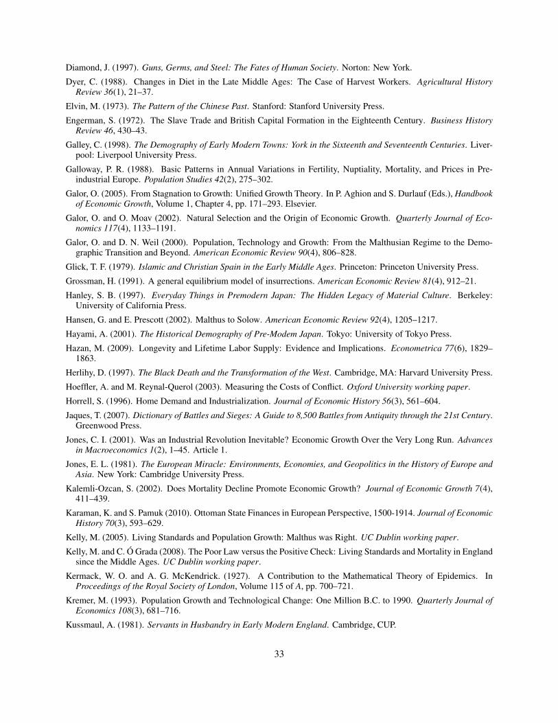
Diamond, J. (1997). Guns, Germs, and Steel: The Fates of Human Society. Norton: New York.
Dyer, C. (1988). Changes in Diet in the Late Middle Ages: The Case of Harvest Workers. Agricultural HistoryReview 36(1), 21–37.
Elvin, M. (1973). The Pattern of the Chinese Past. Stanford: Stanford University Press.
Engerman, S. (1972). The Slave Trade and British Capital Formation in the Eighteenth Century. Business HistoryReview 46, 430–43.
Galley, C. (1998). The Demography of Early Modern Towns: York in the Sixteenth and Seventeenth Centuries. Liver-pool: Liverpool University Press.
Galloway, P. R. (1988). Basic Patterns in Annual Variations in Fertility, Nuptiality, Mortality, and Prices in Pre-industrial Europe. Population Studies 42(2), 275–302.
Galor, O. (2005). From Stagnation to Growth: Unified Growth Theory. In P. Aghion and S. Durlauf (Eds.), Handbookof Economic Growth, Volume 1, Chapter 4, pp. 171–293. Elsevier.
Galor, O. and O. Moav (2002). Natural Selection and the Origin of Economic Growth. Quarterly Journal of Eco-nomics 117(4), 1133–1191.
Galor, O. and D. N. Weil (2000). Population, Technology and Growth: From the Malthusian Regime to the Demo-graphic Transition and Beyond. American Economic Review 90(4), 806–828.
Glick, T. F. (1979). Islamic and Christian Spain in the Early Middle Ages. Princeton: Princeton University Press.
Grossman, H. (1991). A general equilibrium model of insurrections. American Economic Review 81(4), 912–21.
Hanley, S. B. (1997). Everyday Things in Premodern Japan: The Hidden Legacy of Material Culture. Berkeley:University of California Press.
Hansen, G. and E. Prescott (2002). Malthus to Solow. American Economic Review 92(4), 1205–1217.
Hayami, A. (2001). The Historical Demography of Pre-Modem Japan. Tokyo: University of Tokyo Press.
Hazan, M. (2009). Longevity and Lifetime Labor Supply: Evidence and Implications. Econometrica 77(6), 1829–1863.
Herlihy, D. (1997). The Black Death and the Transformation of the West. Cambridge, MA: Harvard University Press.
Hoeffler, A. and M. Reynal-Querol (2003). Measuring the Costs of Conflict. Oxford University working paper.
Horrell, S. (1996). Home Demand and Industrialization. Journal of Economic History 56(3), 561–604.
Jaques, T. (2007). Dictionary of Battles and Sieges: A Guide to 8,500 Battles from Antiquity through the 21st Century.Greenwood Press.
Jones, C. I. (2001). Was an Industrial Revolution Inevitable? Economic Growth Over the Very Long Run. Advancesin Macroeconomics 1(2), 1–45. Article 1.
Jones, E. L. (1981). The European Miracle: Environments, Economies, and Geopolitics in the History of Europe andAsia. New York: Cambridge University Press.
Kalemli-Ozcan, S. (2002). Does Mortality Decline Promote Economic Growth? Journal of Economic Growth 7(4),411–439.
Karaman, K. and S. Pamuk (2010). Ottoman State Finances in European Perspective, 1500-1914. Journal of EconomicHistory 70(3), 593–629.
Kelly, M. (2005). Living Standards and Population Growth: Malthus was Right. UC Dublin working paper.
Kelly, M. and C. Ó Grada (2008). The Poor Law versus the Positive Check: Living Standards and Mortality in Englandsince the Middle Ages. UC Dublin working paper.
Kermack, W. O. and A. G. McKendrick. (1927). A Contribution to the Mathematical Theory of Epidemics. InProceedings of the Royal Society of London, Volume 115 of A, pp. 700–721.
Kremer, M. (1993). Population Growth and Technological Change: One Million B.C. to 1990. Quarterly Journal ofEconomics 108(3), 681–716.
Kussmaul, A. (1981). Servants in Husbandry in Early Modern England. Cambridge, CUP.
33
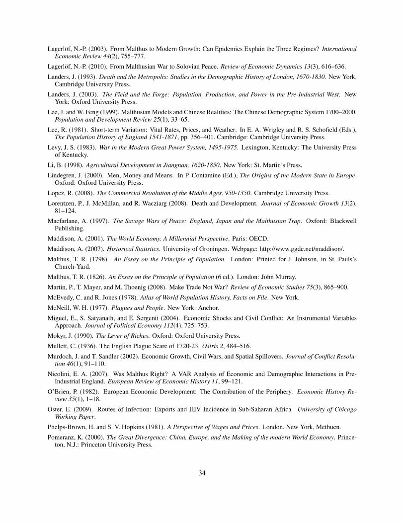
Lagerlöf, N.-P. (2003). From Malthus to Modern Growth: Can Epidemics Explain the Three Regimes? InternationalEconomic Review 44(2), 755–777.
Lagerlöf, N.-P. (2010). From Malthusian War to Solovian Peace. Review of Economic Dynamics 13(3), 616–636.
Landers, J. (1993). Death and the Metropolis: Studies in the Demographic History of London, 1670-1830. New York,Cambridge University Press.
Landers, J. (2003). The Field and the Forge: Population, Production, and Power in the Pre-Industrial West. NewYork: Oxford University Press.
Lee, J. and W. Feng (1999). Malthusian Models and Chinese Realities: The Chinese Demographic System 1700–2000.Population and Development Review 25(1), 33–65.
Lee, R. (1981). Short-term Variation: Vital Rates, Prices, and Weather. In E. A. Wrigley and R. S. Schofield (Eds.),The Population History of England 1541-1871, pp. 356–401. Cambridge: Cambridge University Press.
Levy, J. S. (1983). War in the Modern Great Power System, 1495-1975. Lexington, Kentucky: The University Pressof Kentucky.
Li, B. (1998). Agricultural Development in Jiangnan, 1620-1850. New York: St. Martin’s Press.
Lindegren, J. (2000). Men, Money and Means. In P. Contamine (Ed.), The Origins of the Modern State in Europe.Oxford: Oxford University Press.
Lopez, R. (2008). The Commercial Revolution of the Middle Ages, 950-1350. Cambridge University Press.
Lorentzen, P., J. McMillan, and R. Wacziarg (2008). Death and Development. Journal of Economic Growth 13(2),81–124.
Macfarlane, A. (1997). The Savage Wars of Peace: England, Japan and the Malthusian Trap. Oxford: BlackwellPublishing.
Maddison, A. (2001). The World Economy. A Millennial Perspective. Paris: OECD.
Maddison, A. (2007). Historical Statistics. University of Groningen. Webpage: http://www.ggdc.net/maddison/.
Malthus, T. R. (1798). An Essay on the Principle of Population. London: Printed for J. Johnson, in St. Pauls’sChurch-Yard.
Malthus, T. R. (1826). An Essay on the Principle of Population (6 ed.). London: John Murray.
Martin, P., T. Mayer, and M. Thoenig (2008). Make Trade Not War? Review of Economic Studies 75(3), 865–900.
McEvedy, C. and R. Jones (1978). Atlas of World Population History, Facts on File. New York.
McNeill, W. H. (1977). Plagues and People. New York: Anchor.
Miguel, E., S. Satyanath, and E. Sergenti (2004). Economic Shocks and Civil Conflict: An Instrumental VariablesApproach. Journal of Political Economy 112(4), 725–753.
Mokyr, J. (1990). The Lever of Riches. Oxford: Oxford University Press.
Mullett, C. (1936). The English Plague Scare of 1720-23. Osiris 2, 484–516.
Murdoch, J. and T. Sandler (2002). Economic Growth, Civil Wars, and Spatial Spillovers. Journal of Conflict Resolu-tion 46(1), 91–110.
Nicolini, E. A. (2007). Was Malthus Right? A VAR Analysis of Economic and Demographic Interactions in Pre-Industrial England. European Review of Economic History 11, 99–121.
O’Brien, P. (1982). European Economic Development: The Contribution of the Periphery. Economic History Re-view 35(1), 1–18.
Oster, E. (2009). Routes of Infection: Exports and HIV Incidence in Sub-Saharan Africa. University of ChicagoWorking Paper.
Phelps-Brown, H. and S. V. Hopkins (1981). A Perspective of Wages and Prices. London. New York, Methuen.
Pomeranz, K. (2000). The Great Divergence: China, Europe, and the Making of the modern World Economy. Prince-ton, N.J.: Princeton University Press.
34
Postan, M. M. (1972). The Medieval Economy and Society; an Economic History of Britain, 1100-1500. Berkeley:University of California Press.
Sala-i-Martin, X., G. Doppelhofer, and R. I. Miller (2004). Determinants of Long-Term Growth: A Bayesian Averag-ing of Classical Estimates (BACE) Approach. American Economic Review 94(4), 813–835.
Sharp, P., H. Strulik, and J. Weisdorf (2012). The Determinants of Income in a Malthusian Equilibrium. Journal ofDevelopment Economics 97(1), 112–117.
Slack, P. (1981). The Disappearance of the Plague: An Alternative View. Economic History Review 34(3), 469–476.
Smith, A. (1776). An Inquiry into the Nature and Causes of the Wealth of Nations. Number smith1776 in History ofEconomic Thought Books. McMaster University Archive for the History of Economic Thought.
Stokey, N. L. (2001). A quantitative model of the British industrial revolution, 1780-1850. Carnegie-RochesterConference Series on Public Policy 55(1), 55–109.
Strulik, H. and J. Weisdorf (2008). Population, Food, and Knowledge: A Simple Unified Growth Theory. Journal ofEconomic Growth 13(3), 195–216.
Subramanian, S. and A. Deaton (1996). The Demand for Food and Calories. Journal of Political Economy 104(1),133–162.
Szreter, S. and G. Mooney (1998). Urbanisation, Mortality and the Standard of Living Debate: New Estimates of theExpectation of Life at Birth in Nineteenth-Century British Cities. Economic History Review 50, 84–112.
Tallett, F. (1992). War and Society in Early-Modern Europe, 1495-1715. London: Routledge.
Tilly, C. (1992). Coercion, Capital, and European States, AD 990-1992. Oxford: Blackwells.
Tsui-Jung, L. (1990). Demographic Aspects of Urbanization in the Lower Yangzi Region of China, c. 1500-1900. InA. van der Woude, J. de Vries, and A. Hayami (Eds.), Urbanization in History, pp. 328–351. Oxford: Clarendon.
Voigtländer, N. and H.-J. Voth (2006). Why England? Demographic Factors, Structural Change and Physical CapitalAccumulation during the Industrial Revolution. Journal of Economic Growth 11, 319–361.
Voigtländer, N. and H.-J. Voth (2008). The Three Horsemen of Growth: Plague, War and Urbanization in EarlyModern Europe. UPF manuscript.
Voigtländer, N. and H.-J. Voth (2009). Malthusian Dynamism and the Rise of Europe: Make War, not Love. AmericanEconomic Review, Papers and Proceedings 99(2), 248–54.
Voigtländer, N. and H.-J. Voth (2011). How the West ’Invented’ Fertility Restriction. NBER Working Paper 17314.
Vollrath, D. (2011). The Agricultural Basis of Comparative Development. Journal of Economic Growth 16(4), 343–370.
Weil, D. (2004). Economic Growth. New York: Addison-Wesley.
Weil, D. N. and J. Wilde (2009). How Relevant is Malthus for Economic Development Today? American EconomicReview, Papers and Proceedings 99(2), 255–60.
Wells, H. G. (1905). A Modern Utopia.
Woods, R. (2003). Urban-Rural Mortality Differentials: An Unresolved Debate. Population and Development Re-view 29(1), 29–46.
Wrigley, E. and R. S. Schofield (1981). The Population History of England 1541–1871. Cambridge: CambridgeUniversity Press.
Wrigley, E. A., R. S. Davies, J. E. Oeppen, and R. S. Schofield (1997). English Population History from FamilyReconstitution 1580-1837. New York: Cambridge University Press.
Young, A. (2005). The Gift of the Dying: The Tragedy of AIDS and the Welfare of Future African Generations.Quarterly Journal of Economics 120(2), 423–66.
Ziegler, P. (1969). The Black Death. London: Collins.
35
Figure 1: Steady states in the standard Malthusian model and with ’Horsemen effect’
Steady state in the standard Malthusian model
Wage
Dea
th/B
irth
rate birth rate
death rate
C
wC
Steady states with ’Horsemen effect’
Wage
Dea
th/B
irth
rate
wH
w0
death rate
birth rate
EU
E0
EH
Figure 2: Plague outbreaks and life expectancy
Plague outbreaks in Europe
020
040
060
080
0N
umbe
r of
Out
brea
ks p
er D
ecad
e
1300 1400 1500 1600 1700 1800Year
Life expectancy in early modern England
Data sources: Left panel: Biraben (1975). Data points represent the number of outbreaks over 10 year periods. The solidline is the median of each data point and the two adjacent ones. Right panel: Wrigley and Schofield (1981); 20-year movingaverage.
36
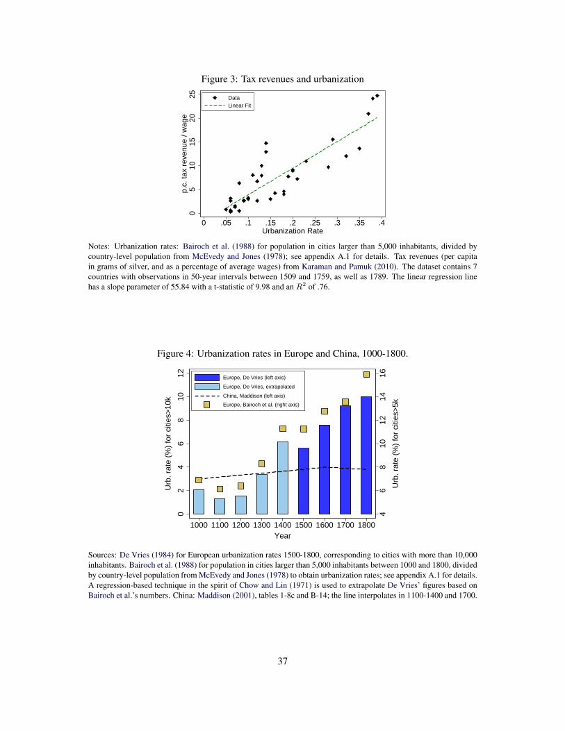
Figure 3: Tax revenues and urbanization
05
1015
2025
p.c.
tax
reve
nue
/ wag
e
0 .05 .1 .15 .2 .25 .3 .35 .4Urbanization Rate
DataLinear Fit
Notes: Urbanization rates: Bairoch et al. (1988) for population in cities larger than 5,000 inhabitants, divided bycountry-level population from McEvedy and Jones (1978); see appendix A.1 for details. Tax revenues (per capitain grams of silver, and as a percentage of average wages) from Karaman and Pamuk (2010). The dataset contains 7countries with observations in 50-year intervals between 1509 and 1759, as well as 1789. The linear regression linehas a slope parameter of 55.84 with a t-statistic of 9.98 and an R2 of .76.
Figure 4: Urbanization rates in Europe and China, 1000-1800.
46
810
1214
16
Urb
. rat
e (%
) fo
r ci
ties>
5k
02
46
810
12
Urb
. rat
e (%
) fo
r ci
ties>
10k
1000 1100 1200 1300 1400 1500 1600 1700 1800Year
Europe, De Vries (left axis)
Europe, De Vries, extrapolated
China, Maddison (left axis)
Europe, Bairoch et al. (right axis)
Sources: De Vries (1984) for European urbanization rates 1500-1800, corresponding to cities with more than 10,000inhabitants. Bairoch et al. (1988) for population in cities larger than 5,000 inhabitants between 1000 and 1800, dividedby country-level population from McEvedy and Jones (1978) to obtain urbanization rates; see appendix A.1 for details.A regression-based technique in the spirit of Chow and Lin (1971) is used to extrapolate De Vries’ figures based onBairoch et al.’s numbers. China: Maddison (2001), tables 1-8c and B-14; the line interpolates in 1100-1400 and 1700.
37
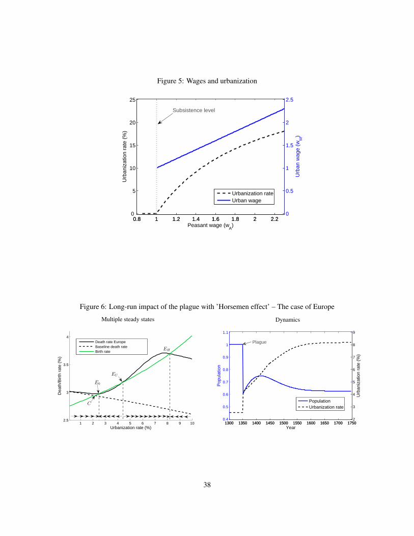
Figure 5: Wages and urbanization
0.8 1 1.2 1.4 1.6 1.8 2 2.20
5
10
15
20
25
Urb
aniz
atio
n ra
te (
%)
Peasant wage (wA)
0.8 1 1.2 1.4 1.6 1.8 2 2.20
0.5
1
1.5
2
2.5
Urb
an w
age
(wM
)
Urbanization rateUrban wage
Subsistence level
Figure 6: Long-run impact of the plague with ’Horsemen effect’ – The case of Europe
Multiple steady states
1 2 3 4 5 6 7 8 9 102.5
3
3.5
4
Urbanization rate (%)
Dea
th/B
irth
rate
(%
)
Death rate EuropeBaseline death rateBirth rate
EU
EH
E0
C
Dynamics
1300 1350 1400 1450 1500 1550 1600 1650 1700 17500.4
0.5
0.6
0.7
0.8
0.9
1
1.1
Pop
ulat
ion
Year
1300 1350 1400 1450 1500 1550 1600 1650 1700 17502
3
4
5
6
7
8
9
Urb
aniz
atio
n ra
te (
%)
PopulationUrbanization rate
Plague
38

Figure 7: Effect of ongoing technological progress
Steady state with ongoing TFP growth
1 2 3 4 5 6 7 8 9 102.5
3
3.5
4
Urbanization rate (%)
Dea
th/B
irth
Rat
e (%
)
Birth RateDeath Rate
C b − d =γA
1−β
T
Dynamics
1300 1350 1400 1450 1500 1550 1600 1650 1700 1750
1
1.3
1.6
1.9
2.2
2.5
2.8
Pop
ulat
ion
Year
1300 1350 1400 1450 1500 1550 1600 1650 1700 17502
3
4
5
6
7
8
9
Urb
aniz
atio
n ra
te (
%)Population
Urbanization rate
Figure 8: Europe: Simulation results vs. data
Population (1000 AD = 1)
1000 1100 1200 1300 1400 1500 1600 1700
1
1.5
2
2.5
3
3.5
4
Year
Inde
x
SimulationData
Urbanization Rate
1000 1100 1200 1300 1400 1500 1600 17000
1
2
3
4
5
6
7
8
9
10
Year
Per
cent
SimulationDe VriesDe Vries − extrapolated
Data sources: Population for Europe (exclusive of the Balkans and Russia) from McEvedy and Jones (1978). Urban-ization rates: For 1500-1700 from de Vries (1984); 1000-1400: De Vries (1984), extrapolated using data from Bairochet al. (1988). See the notes below figure 4 and appendix A.1 for details.
39
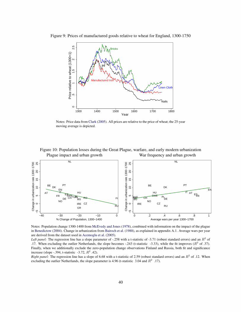
Figure 9: Prices of manufactured goods relative to wheat for England, 1300-1750
Bricks
Linen Cloth
Nails
Manufactured Iron
0.5
11.
52
2.5
Pric
e re
lativ
e to
whe
at (
1300
=1)
1300 1400 1500 1600 1700 1800Year
Notes: Price data from Clark (2005). All prices are relative to the price of wheat; the 25-yearmoving average is depicted.
Figure 10: Population losses during the Great Plague, warfare, and early modern urbanizationPlague impact and urban growth
DE
AT
BE
BG
DK
ES
FIFR
EN
GR
HU
IRE
IT
NO
NL
PL
PT
RO
RU
SWECH
CZ
YUG
−5
05
1015
2025
Cha
nge
in u
rban
izat
ion
rate
130
0−17
00
−40 −30 −20 −10 0% Change of Population, 1300−1400
War frequency and urban growth
DE
AT
BE
BG
DK
ESFR
ENHU
IRE
IT
NO
NL
PL
PT
RO
RU
SWECH
CZ
YUG
−5
05
1015
2025
Cha
nge
in u
rban
izat
ion
rate
130
0−17
00
0 .2 .4 .6 .8 1Average wars per year 1300−1700
Notes: Population change 1300-1400 from McEvedy and Jones (1978), combined with information on the impact of the plaguein Benedictow (2004). Change in urbanization from Bairoch et al. (1988), as explained in appendix A.1. Average wars per yearare derived from the dataset used in Acemoglu et al. (2005).Left panel: The regression line has a slope parameter of -.258 with a t-statistic of -3.71 (robust standard errors) and an R2 of.17. When excluding the outlier Netherlands, the slope becomes -.243 (t-statistic -3.33), while the fit improves (R2 of .37).Finally, when we additionally exclude the zero-population change observations Finland and Russia, both fit and significanceincrease (slope -.394, t-statistic -3.72, R2 .42).Right panel: The regression line has a slope of 6.68 with a t-statistic of 2.59 (robust standard errors) and an R2 of .12. Whenexcluding the outlier Netherlands, the slope parameter is 4.96 (t-statistic 3.04 and R2 .17).
40