the three-body problemsome interesting dynamics inperiodic

Periodic Orbits and Transport:Some Interesting Dynamics in

the Three-Body Problem

Shane RossMartin Lo (JPL), Wang Sang Koon and Jerrold Marsden (Caltech)

CDS 280, January 8, 2001

[email protected]://www.cds.caltech.edu/˜shane/

Control and Dynamical Systems

2

Outline

• Important dynamical objects : Equilibria, periodic orbits,stable and unstable manifolds, bottlenecks

•Context : Three-body problem (Hamiltonian)

• Equilibria : Collinear libration points have saddle × centerstructure

•Periodic orbits : Stable and unstable invariant manifolds divideenergy surface, channeling flow in phase space

•Classification : Interesting orbits can be classified and con-structed using Poincare sections and symbolic dynamics

•Theorem : Near home/heteroclinic orbits, “horseshoe”-like dy-namics exists

•Application : Actual space missions

5

Connecting Orbits

� Simple Pendulum

• Equations of a simple pendulum are θ + sin θ = 0.

• Write as a system in the plane ;

dθ

dt= v

dv

dt= − sin θ

• Solutions are trajectories in the plane.

• The resulting phase portrait shows some important basic fea-tures:

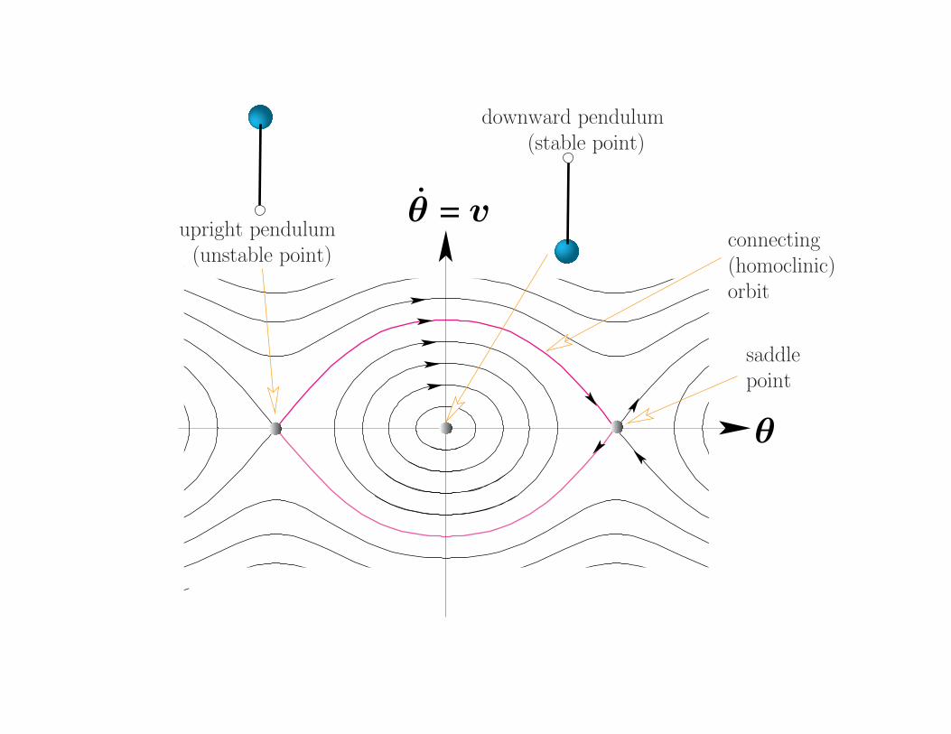
connecting (homoclinic) orbit

saddlepoint

upright pendulum (unstable point)

downward pendulum (stable point)

θ

θ = v

7

� Higher Dimensional Versions are Invariant Manifolds

Stable Manifold

Unstable Manifold

8

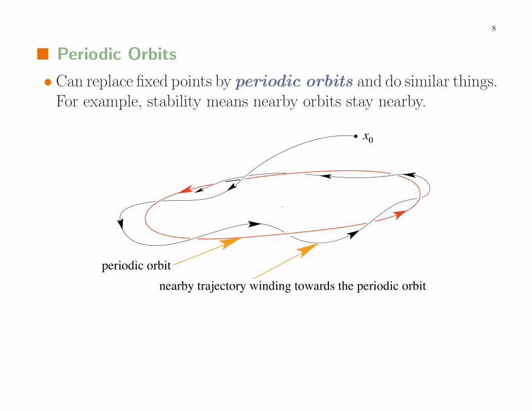
� Periodic Orbits

• Can replace fixed points by periodic orbits and do similar things.For example, stability means nearby orbits stay nearby.

x0

periodic orbit

nearby trajectory winding towards the periodic orbit

9

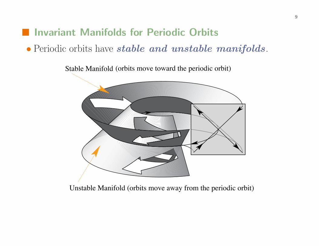
� Invariant Manifolds for Periodic Orbits

• Periodic orbits have stable and unstable manifolds .

Unstable Manifold (orbits move away from the periodic orbit)

Stable Manifold (orbits move toward the periodic orbit)

3

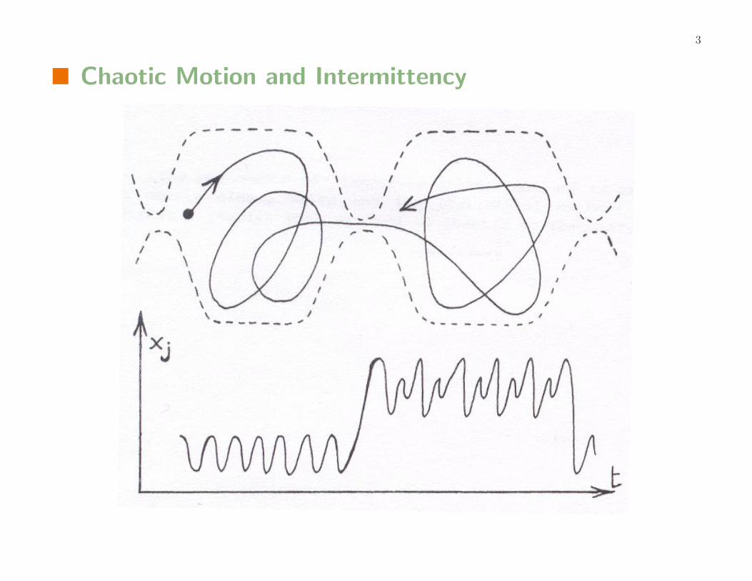
� Chaotic Motion and Intermittency

4

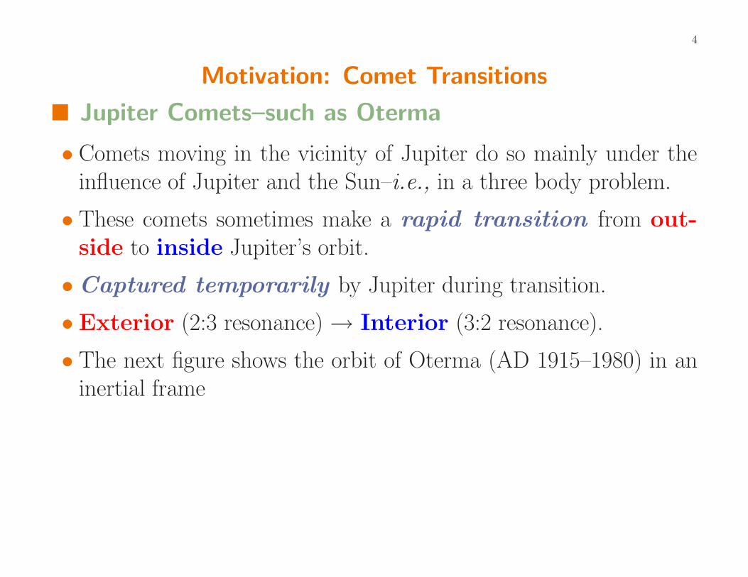
Motivation: Comet Transitions

� Jupiter Comets–such as Oterma

• Comets moving in the vicinity of Jupiter do so mainly under theinfluence of Jupiter and the Sun–i.e., in a three body problem.

• These comets sometimes make a rapid transition from out-side to inside Jupiter’s orbit.

•Captured temporarily by Jupiter during transition.

• Exterior (2:3 resonance)→ Interior (3:2 resonance).

• The next figure shows the orbit of Oterma (AD 1915–1980) in aninertial frame

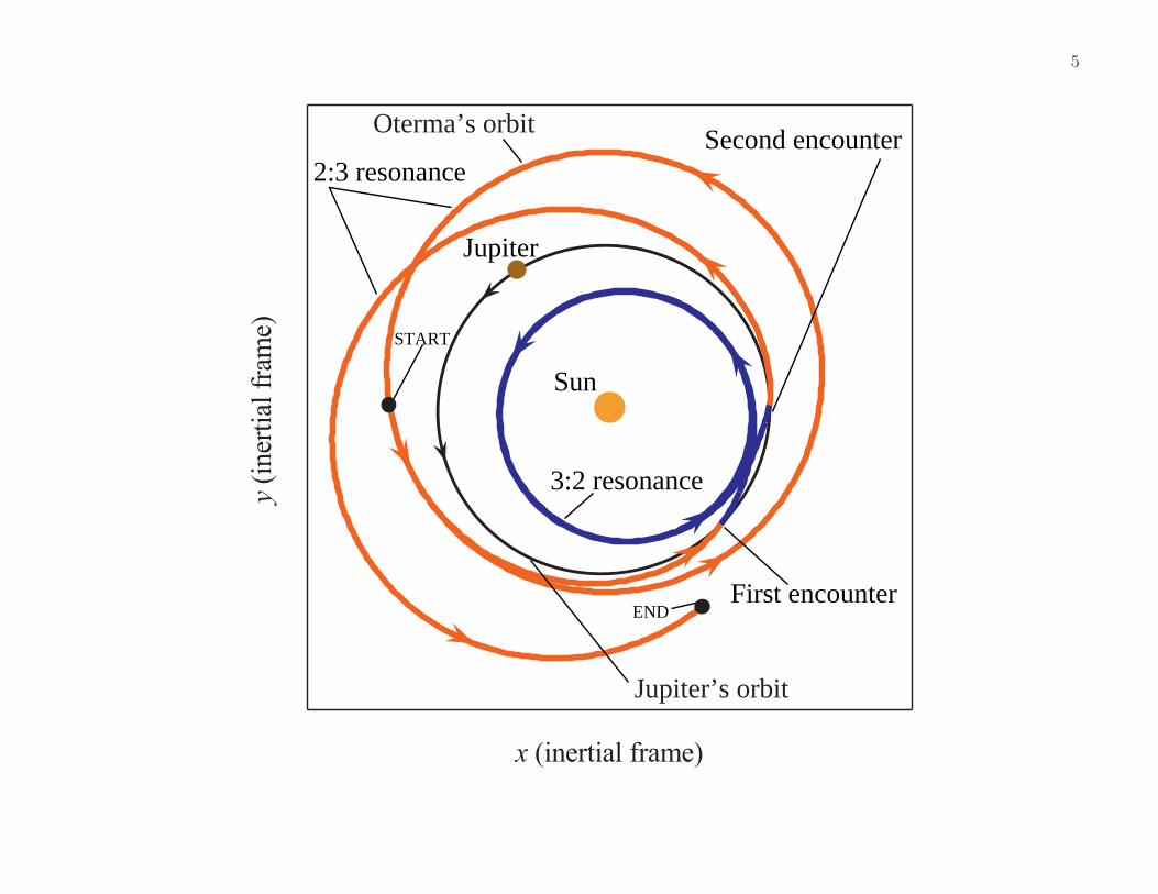
5

x (inertial frame)

y(inertialframe)

Jupiter’s orbit

Sun

END

START

First encounter

Second encounter

3:2 resonance

2:3 resonance

Oterma’s orbit

Jupiter

6

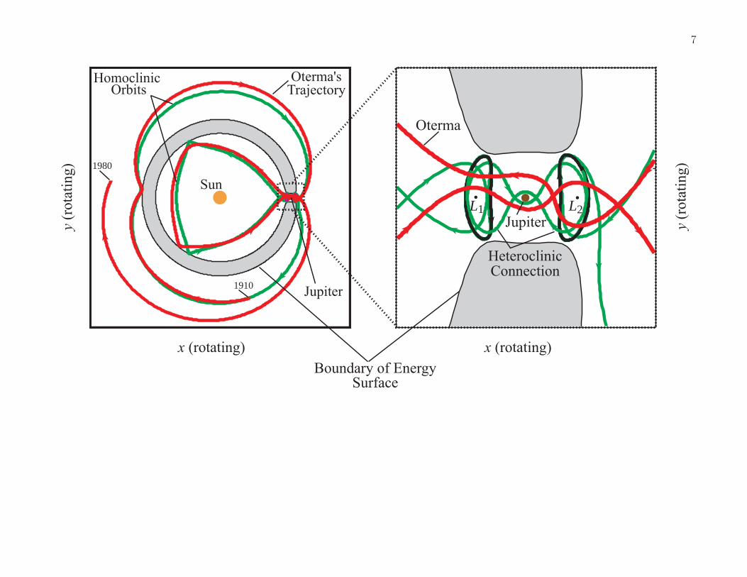
• Next figure shows Oterma’s orbit in a rotating frame (so Jupiterlooks like it is standing still) and with some invariant manifolds inthe three body problem superimposed.

7

y (

rota

ting)

x (rotating)

L1

y (

rota

ting)

x (rotating)

L2Jupiter

Sun

Jupiter

Boundary of EnergySurface

Homoclinic Orbits

1980

1910

Oterma'sTrajectory

HeteroclinicConnection

Oterma

8

Movie: Oterma in arotating frame

9

Planar Circular Restricted 3-Body Problem–PCR3BP

� General Comments

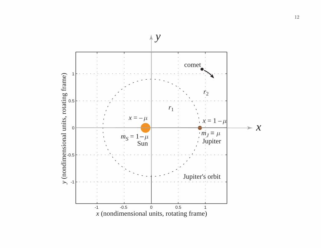
• The two main bodies could be the Sun and Jupiter , or theSun and Earth , etc. The total mass is normalized to 1; theyare denoted mS = 1− µ and mJ = µ, so 0 < µ ≤ 1

2.

◦ The two main bodies rotate in the plane in circles counterclock-wise about their common center of mass and with angular ve-locity normalized to 1.◦ The third body, the comet or the spacecraft , has mass zero

and is free to move in the plane.

• The planar restricted three-body problem is used for simplicity.Generalization to the three-dimensional problem is of courseimportant, but many of the effects can be described well with theplanar model.

10

� Equations of Motion

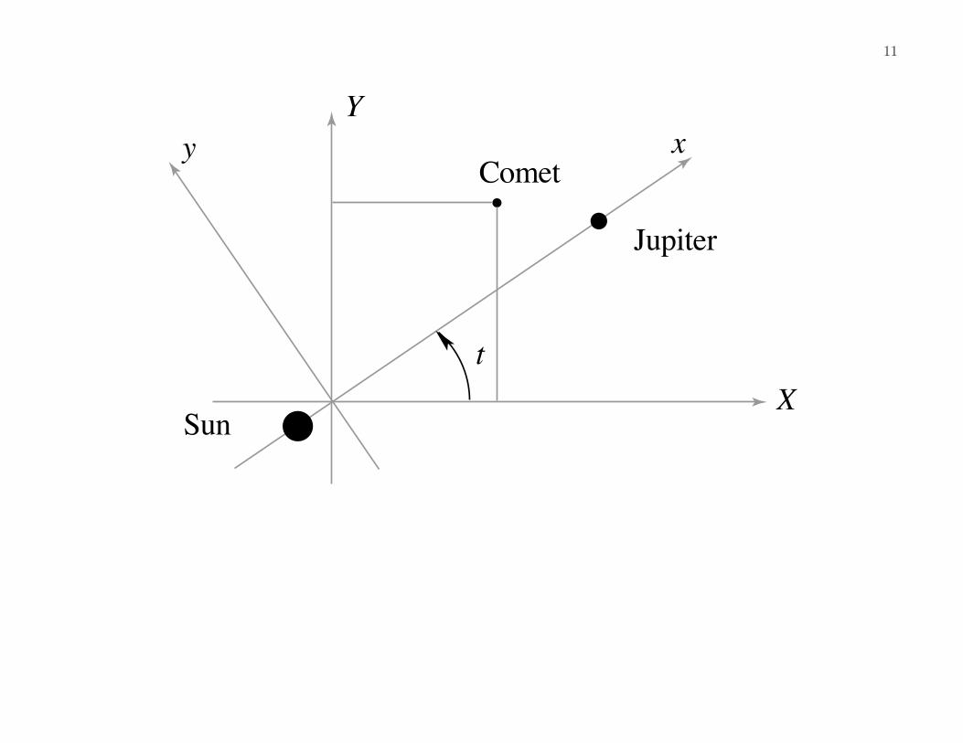
•Notation: Choose a rotating coordinate system so that

◦ the origin is at the center of mass◦ the Sun and Jupiter are on the x-axis at the points (−µ, 0) and

(1−µ, 0) respectively–i.e., the distance from the Sun to Jupiteris normalized to be 1.◦ Let (x, y) be the position of the comet in the plane relative to

the positions of the Sun and Jupiter.◦ distances to the Sun and Jupiter:

r1 =√

(x + µ)2 + y2 and r2 =√

(x− 1 + µ)2 + y2.

11

Y

X

xy

Jupiter

Sun

t

Comet

12

-1 -0.5 0 0.5 1

-1

-0.5

0

0.5

1

x (nondimensional units, rotating frame)

y (n

ondi

men

sion

al u

nits

, rot

atin

g fr

ame)

mS = 1 – µ mJ = µ

Sun

Jupiter's orbit

comet

x = – µ

Jupiter

x = 1 – µ

r1

r2

y

x

13

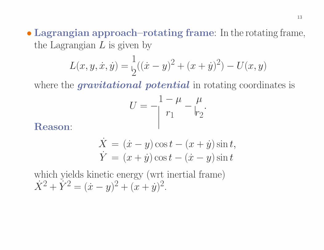
• Lagrangian approach–rotating frame: In the rotating frame,the Lagrangian L is given by

L(x, y, x, y) =12

((x− y)2 + (x + y)2)− U(x, y)

where the gravitational potential in rotating coordinates is

U = −1− µr1− µ

r2.

Reason:

X = (x− y) cos t− (x + y) sin t,Y = (x + y) cos t− (x− y) sin t

which yields kinetic energy (wrt inertial frame)X2 + Y 2 = (x− y)2 + (x + y)2.

14

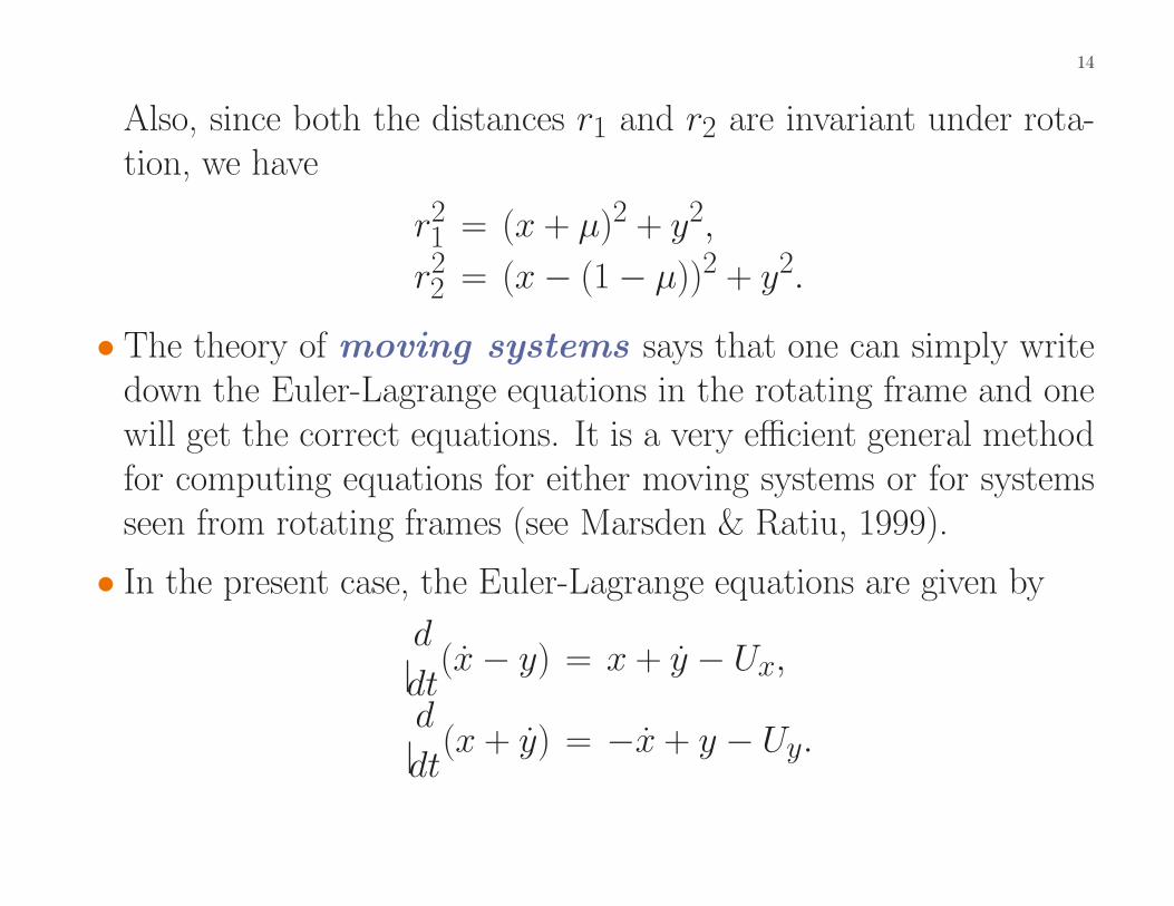
Also, since both the distances r1 and r2 are invariant under rota-tion, we have

r21 = (x + µ)2 + y2,

r22 = (x− (1− µ))2 + y2.

• The theory of moving systems says that one can simply writedown the Euler-Lagrange equations in the rotating frame and onewill get the correct equations. It is a very efficient general methodfor computing equations for either moving systems or for systemsseen from rotating frames (see Marsden & Ratiu, 1999).

• In the present case, the Euler-Lagrange equations are given byd

dt(x− y) = x + y − Ux,

d

dt(x + y) = −x+ y − Uy.

15

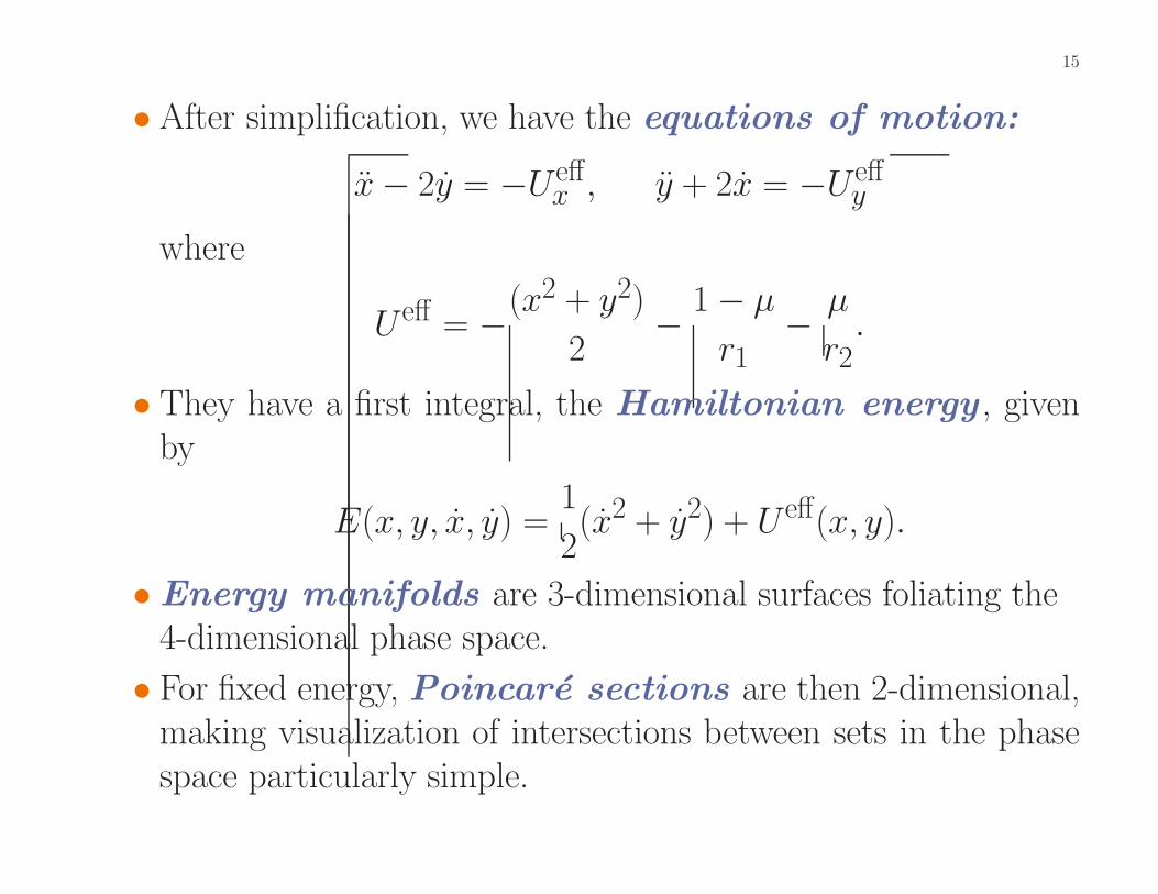
• After simplification, we have the equations of motion:

x− 2y = −Ueffx , y + 2x = −Ueff

y

where

U eff = −(x2 + y2)2

− 1− µr1− µ

r2.

• They have a first integral, the Hamiltonian energy , givenby

E(x, y, x, y) =12

(x2 + y2) + U eff(x, y).

• Energy manifolds are 3-dimensional surfaces foliating the4-dimensional phase space.• For fixed energy, Poincare sections are then 2-dimensional,

making visualization of intersections between sets in the phasespace particularly simple.

16

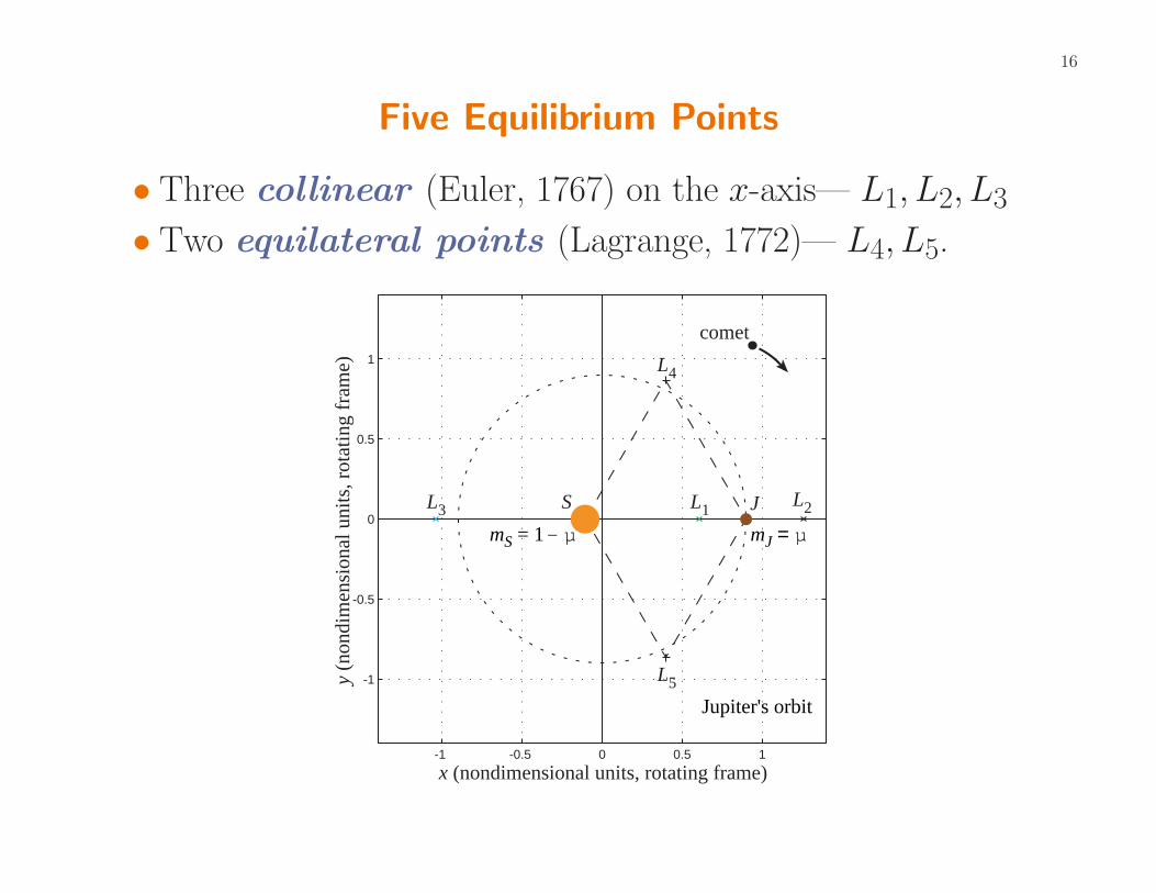
Five Equilibrium Points

• Three collinear (Euler, 1767) on the x-axis— L1, L2, L3• Two equilateral points (Lagrange, 1772)— L4, L5.

-1 -0.5 0 0.5 1

-1

-0.5

0

0.5

1

x (nondimensional units, rotating frame)

y (n

ondi

men

sion

al u

nits

, rot

atin

g fr

ame)

mS = 1 - µ mJ = µ

S J

Jupiter's orbit

L2

L4

L5

L3 L1

comet

17

Energy Manifold

• The energy E is given by

E(x, y, x, y) =12

(x2 + y2) + U eff(x, y)

=12

(x2 + y2)− 12

(x2 + y2)− 1− µr1− µ

r2.

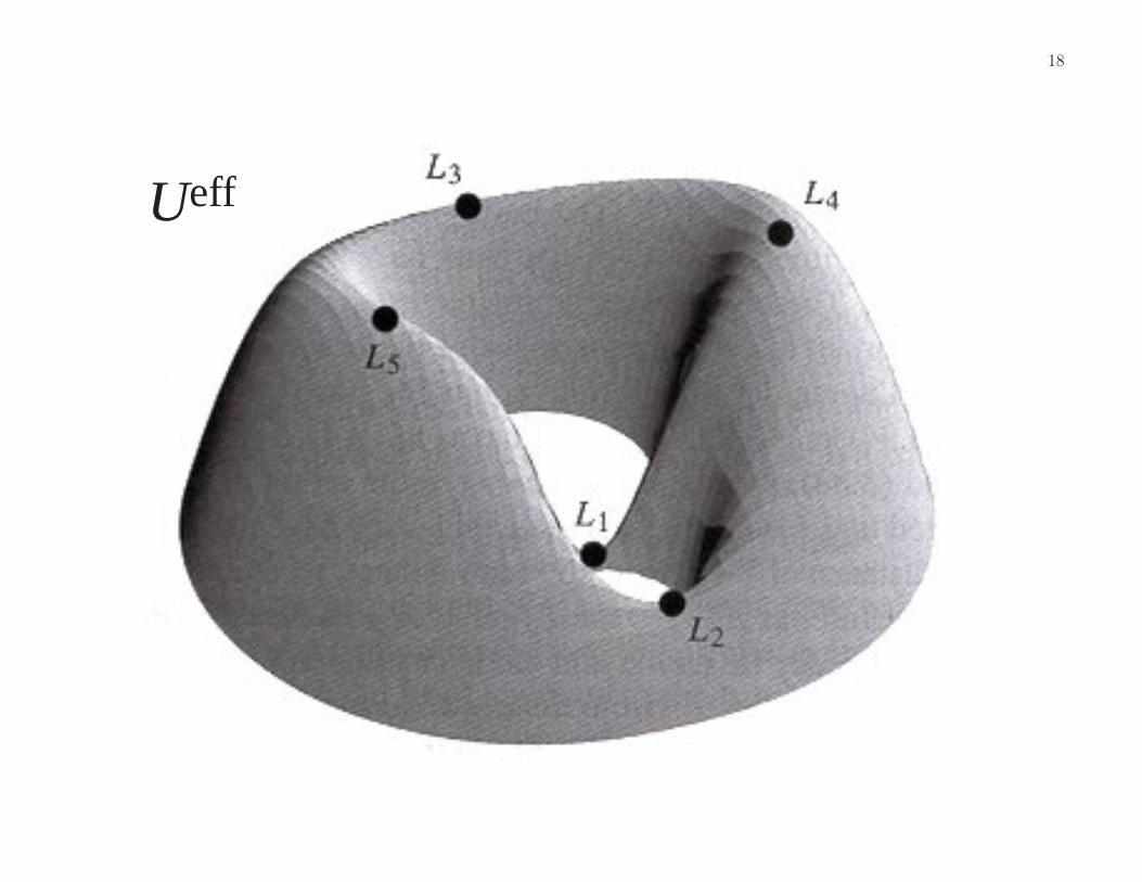
This energy integral will help us determine the region of pos-sible motion , i.e., the region in which the comet can possiblymove along and the region which it is forbidden to move. Thefirst step is to look at the surface of the effective potential U eff.• Note that the energy manifold is 3-dimensional.

18

Ueff

19

◦ Near either the Sun or Jupiter, we have a potential well.◦ Far away from the Sun-Jupiter system, the term that corre-

sponds to the centrifugal force dominates, we have anotherpotential well.◦Moreover, by applying multivariable calculus, one finds that

there are 3 saddle points at L1, L2, L3 and 2 maxima at L4and L5.◦ Let Ei be the energy at Li, then E5 = E4 > E3 > E2 > E1.

20

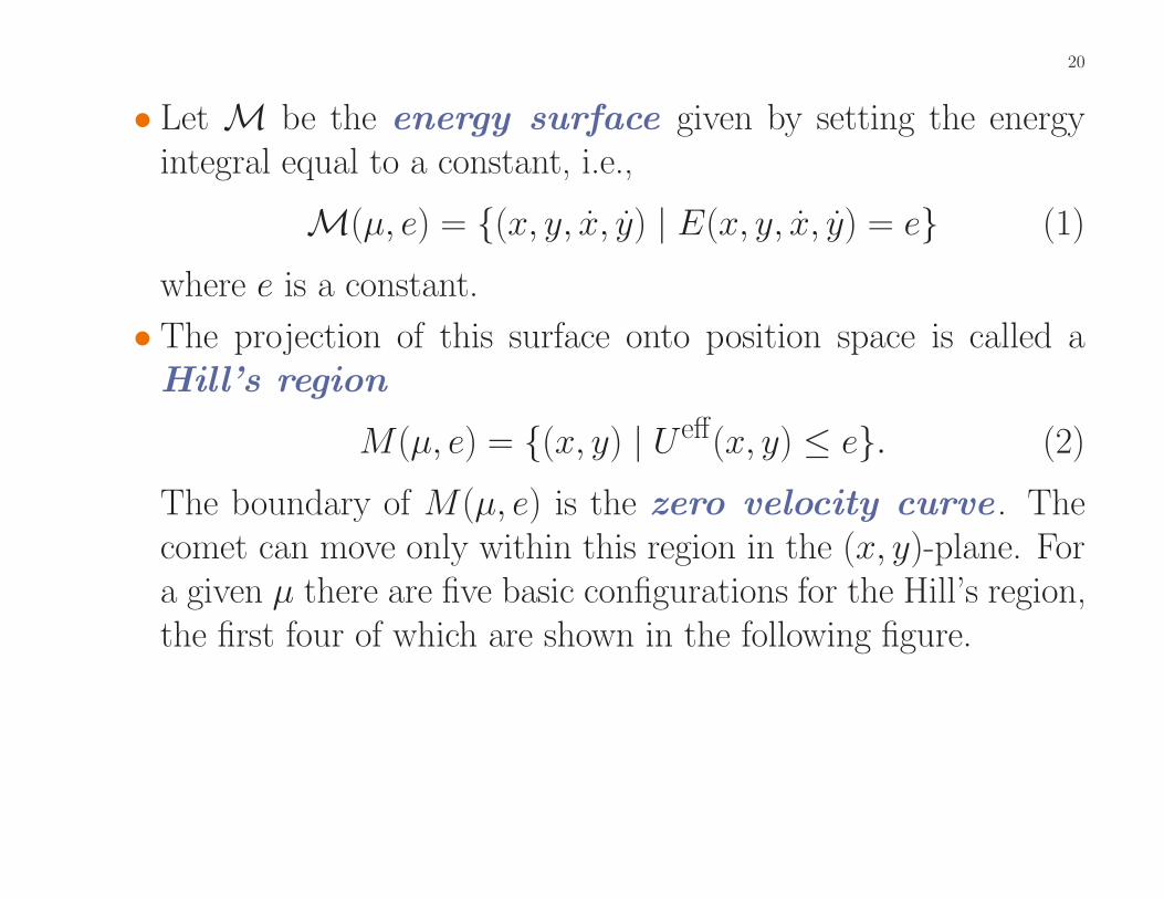
• Let M be the energy surface given by setting the energyintegral equal to a constant, i.e.,

M(µ, e) = {(x, y, x, y) | E(x, y, x, y) = e} (1)

where e is a constant.• The projection of this surface onto position space is called a

Hill’s region

M(µ, e) = {(x, y) | U eff(x, y) ≤ e}. (2)

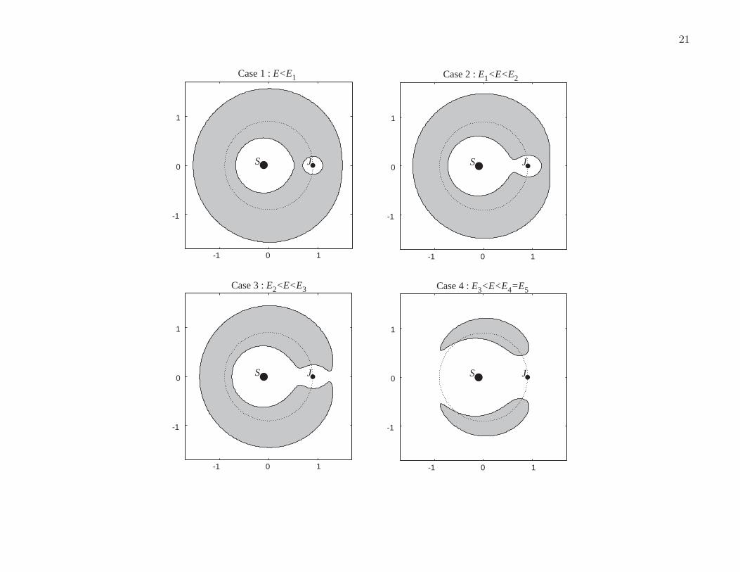
The boundary of M(µ, e) is the zero velocity curve . Thecomet can move only within this region in the (x, y)-plane. Fora given µ there are five basic configurations for the Hill’s region,the first four of which are shown in the following figure.

21

-1 0 1

-1

0

1

-1 0 1

-1

0

1

-1 0 1

-1

0

1

-1 0 1

-1

0

1

S J S J

S JS J

Case 1 : E<E1 Case 2 : E1<E<E2

Case 4 : E3<E<E4=E5Case 3 : E2<E<E3

22

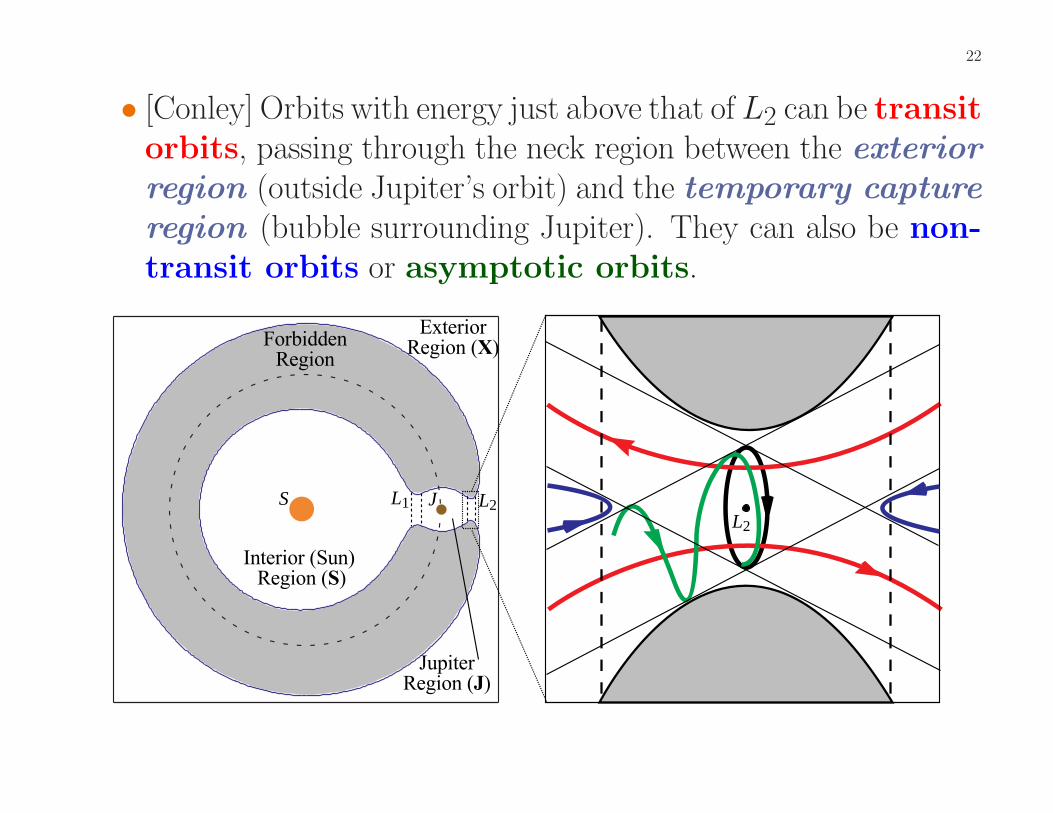
• [Conley] Orbits with energy just above that of L2 can be transitorbits, passing through the neck region between the exteriorregion (outside Jupiter’s orbit) and the temporary captureregion (bubble surrounding Jupiter). They can also be non-transit orbits or asymptotic orbits.

S JL1 L2

ExteriorRegion (X)

Interior (Sun)Region (S)

JupiterRegion (J)

ForbiddenRegion

L2

23

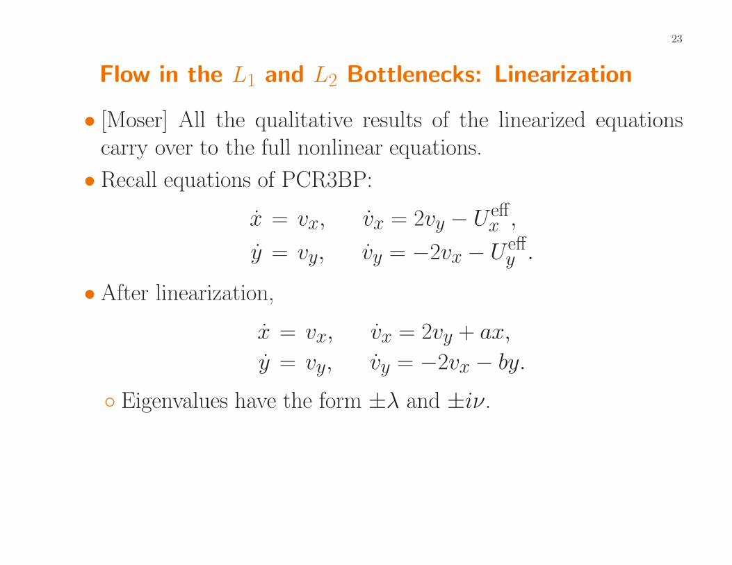
Flow in the L1 and L2 Bottlenecks: Linearization

• [Moser] All the qualitative results of the linearized equationscarry over to the full nonlinear equations.• Recall equations of PCR3BP:

x = vx, vx = 2vy − U effx ,

y = vy, vy = −2vx − Ueffy .

• After linearization,

x = vx, vx = 2vy + ax,

y = vy, vy = −2vx − by.◦ Eigenvalues have the form ±λ and ±iν.

24

◦ Corresponding eigenvectors are

u1 = (1,−σ, λ,−λσ),u2 = (1, σ,−λ,−λσ),w1 = (1,−iτ, iν, ντ ),w2 = (1, iτ,−iν, ντ ).

25

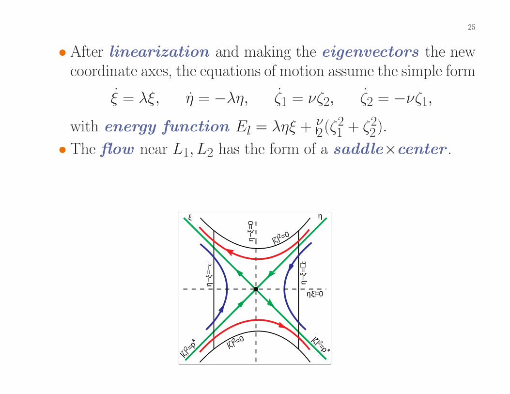
• After linearization and making the eigenvectors the newcoordinate axes, the equations of motion assume the simple form

ξ = λξ, η = −λη, ζ1 = νζ2, ζ2 = −νζ1,

with energy function El = ληξ + ν2(ζ2

1 + ζ22).

• The flow near L1, L2 has the form of a saddle×center .

η−ξ=

−c

η−ξ=

+c

η−ξ=

0

η+ξ=0

|ζ|2 =0

ξ η

|ζ|2 =ρ∗

|ζ| 2=ρ ∗|ζ|2 =0

26

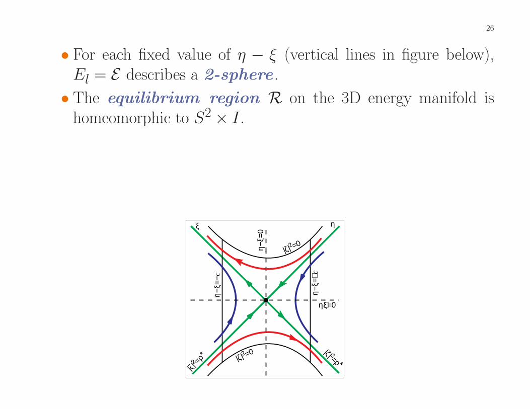
• For each fixed value of η − ξ (vertical lines in figure below),El = E describes a 2-sphere .• The equilibrium region R on the 3D energy manifold is

homeomorphic to S2 × I.

η−ξ=

−c

η−ξ=

+c

η−ξ=

0

η+ξ=0

|ζ|2 =0

ξ η

|ζ|2 =ρ∗

|ζ| 2=ρ ∗|ζ|2 =0

27

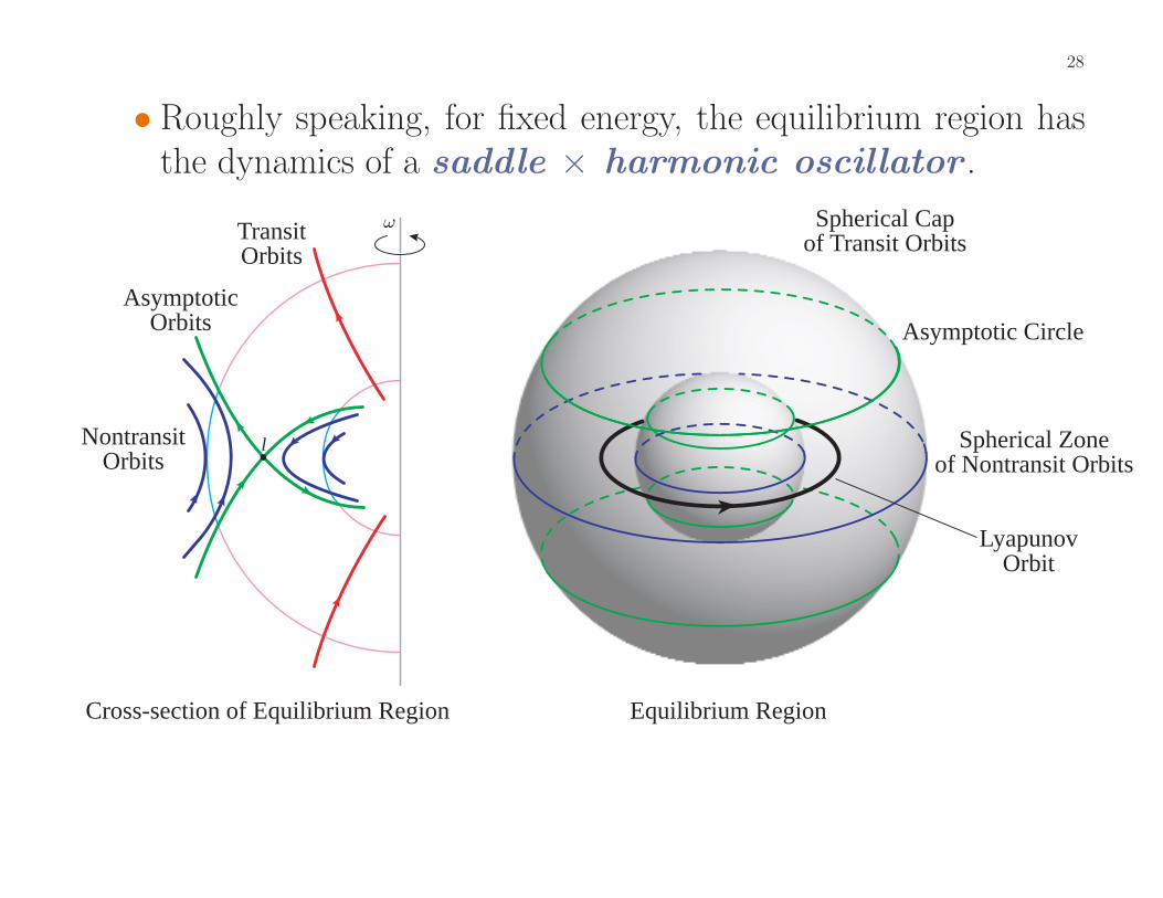
• [McGehee] Can visualize 4 types of orbits in R ' S2 × I.◦Black circle is the unstable periodic Lyapunov orbit.◦ 4 cylinders of asymptotic orbits form pieces of stable and

unstable manifolds. They intersect the bounding spheres atasymptotic circles, separating spherical polar caps , whichcontain transit orbits, from spherical equatorial zones ,which contain nontransit orbits.

LyapunovOrbit

ω

l

TransitOrbits

AsymptoticOrbits

NontransitOrbits

Spherical Capof Transit Orbits

Spherical Zoneof Nontransit Orbits

Asymptotic Circle

Cross-section of Equilibrium Region Equilibrium Region

28

• Roughly speaking, for fixed energy, the equilibrium region hasthe dynamics of a saddle × harmonic oscillator .

LyapunovOrbit

ω

l

TransitOrbits

AsymptoticOrbits

NontransitOrbits

Spherical Capof Transit Orbits

Spherical Zoneof Nontransit Orbits

Asymptotic Circle

Cross-section of Equilibrium Region Equilibrium Region

29

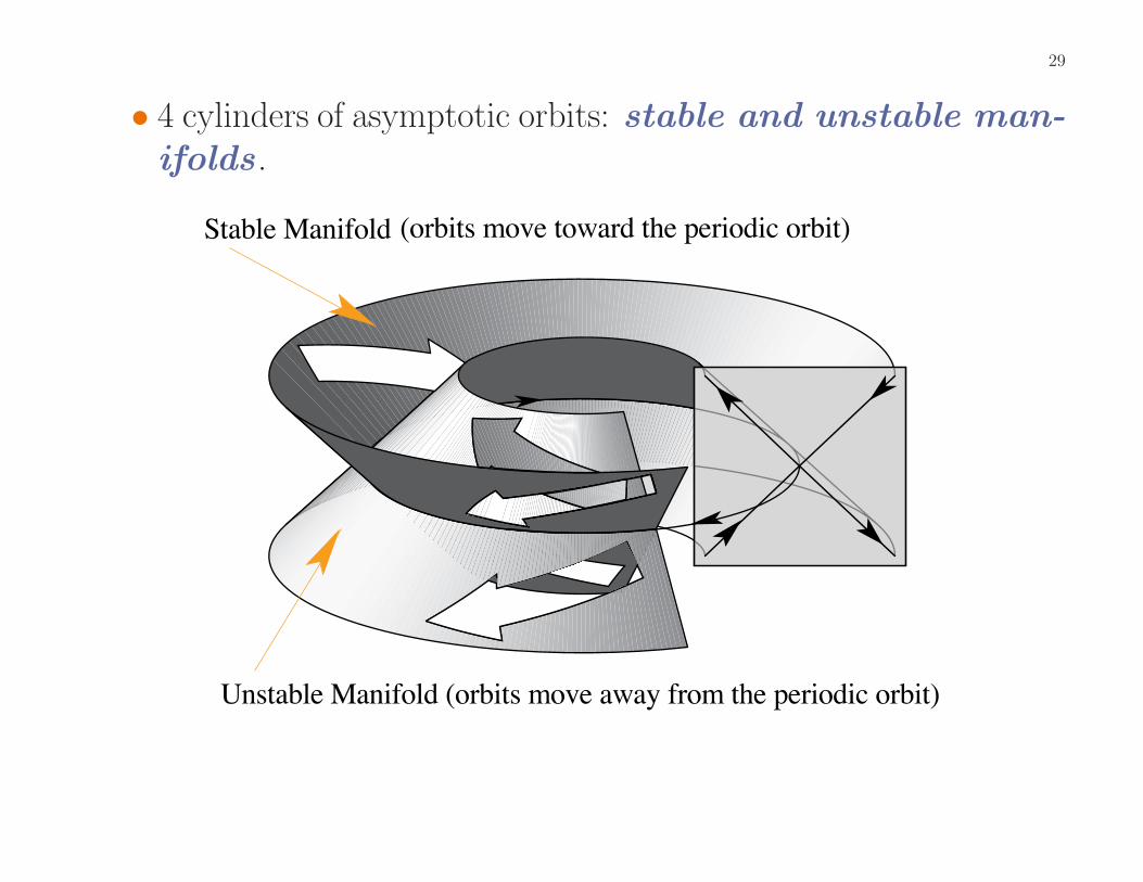
• 4 cylinders of asymptotic orbits: stable and unstable man-ifolds .

Unstable Manifold (orbits move away from the periodic orbit)

Stable Manifold (orbits move toward the periodic orbit)

30

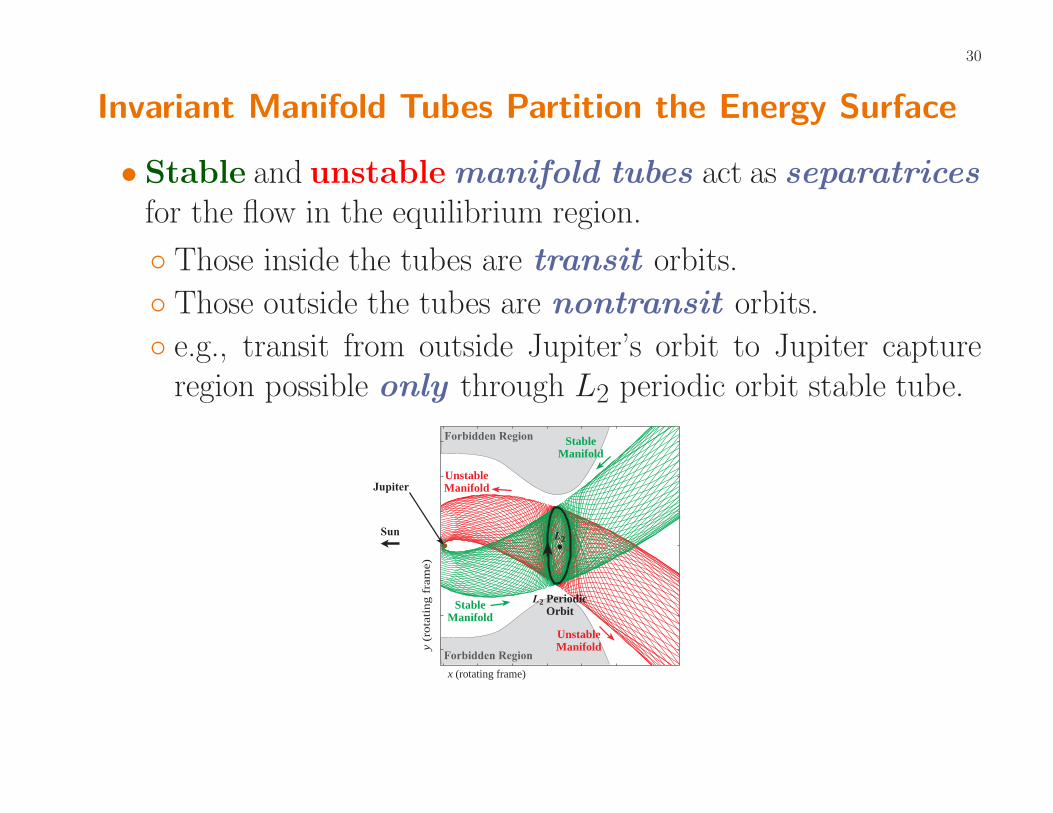
Invariant Manifold Tubes Partition the Energy Surface

• Stable and unstable manifold tubes act as separatricesfor the flow in the equilibrium region.◦ Those inside the tubes are transit orbits.◦ Those outside the tubes are nontransit orbits.◦ e.g., transit from outside Jupiter’s orbit to Jupiter capture

region possible only through L2 periodic orbit stable tube.

x (rotating frame)

y (r

ota

tin

g f

ram

e)

L2 PeriodicOrbitStable

Manifold

UnstableManifold

Sun

StableManifold

Forbidden Region

UnstableManifold

Jupiter

Forbidden Region

L2

31

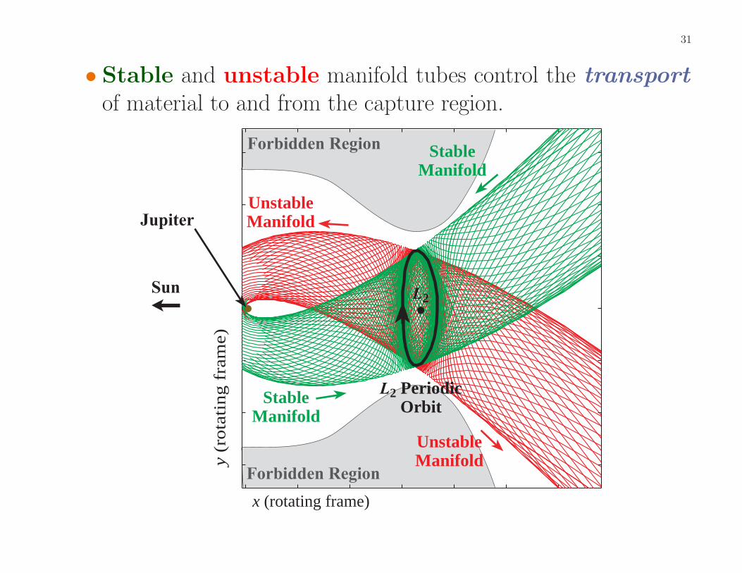
• Stable and unstable manifold tubes control the transportof material to and from the capture region.

x (rotating frame)

y (r

ota

tin

g f

ram

e)

L2 PeriodicOrbitStable

Manifold

UnstableManifold

Sun

StableManifold

Forbidden Region

UnstableManifold

Jupiter

Forbidden Region

L2

32

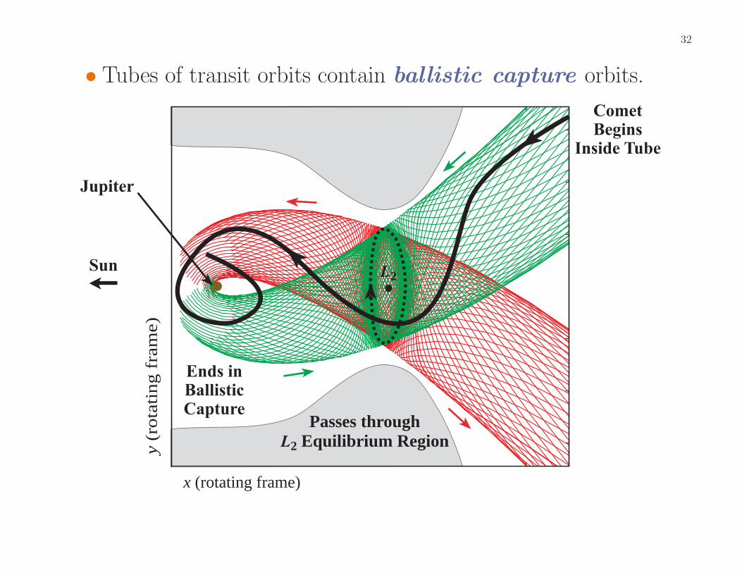
• Tubes of transit orbits contain ballistic capture orbits.

Passes throughL2 Equilib r ium Region

L2

Ends inBallisticCapture

CometBegins

Inside Tube

x (rotating frame)

y (r

ota

tin

g f

ram

e)

Sun

Jupiter

33

• Invariant manifold tubes are global objects — extend far be-yond vicinity of libration points.

Sun L2 orbit

Jupiter

ForbiddenRegion

Tube of TransitOrbits

CaptureOrbit

x (rotating frame)

y (

rota

ting f

rame)

34

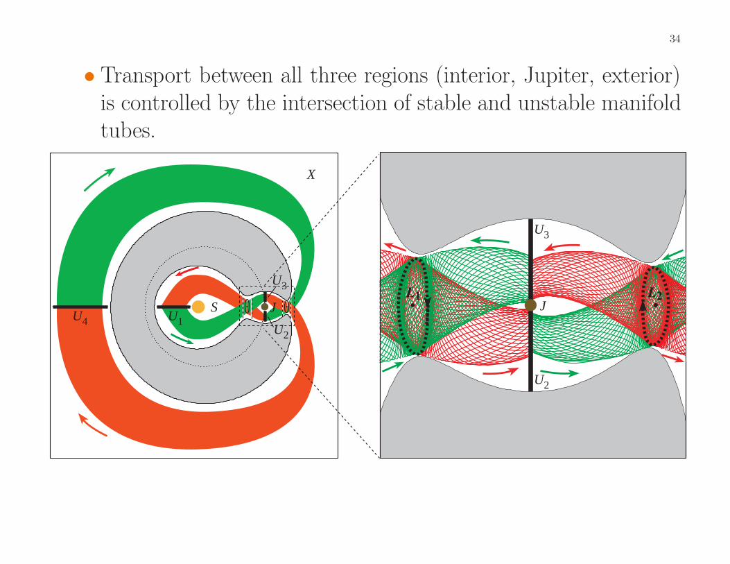
• Transport between all three regions (interior, Jupiter, exterior)is controlled by the intersection of stable and unstable manifoldtubes.

X

S JL1 L2

J

U3

U2

U1U4

U3

U2

35

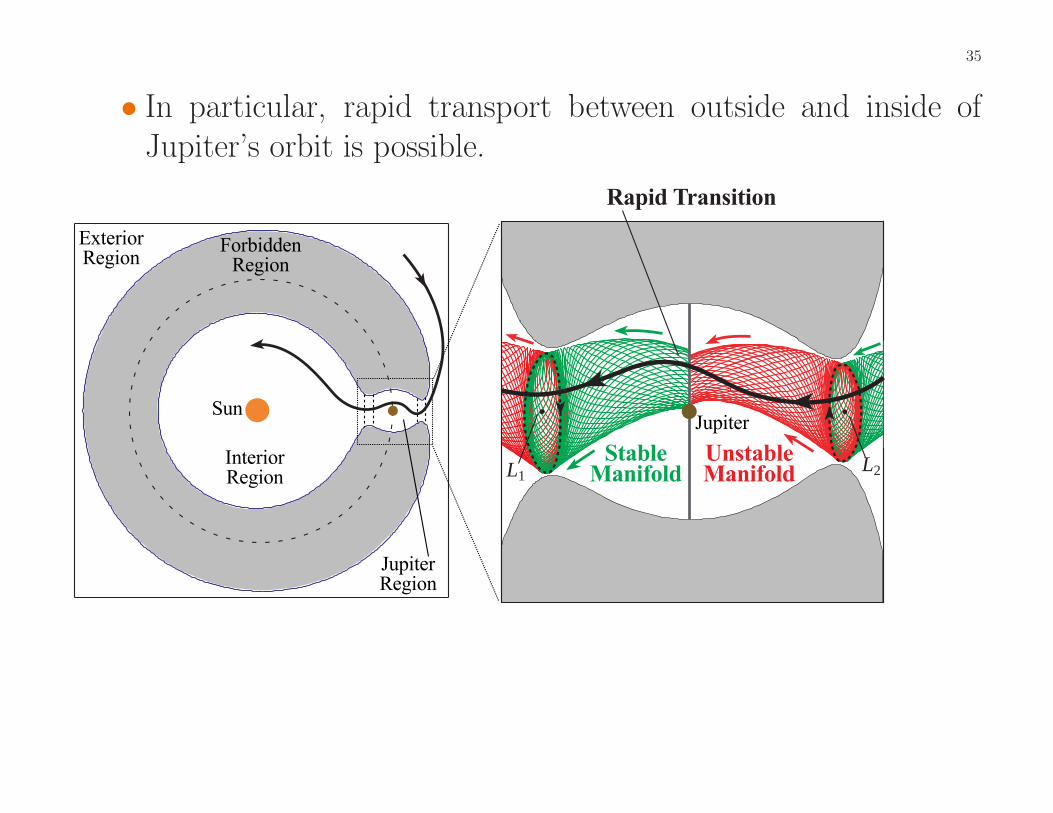
• In particular, rapid transport between outside and inside ofJupiter’s orbit is possible.

ExteriorRegion

InteriorRegion

JupiterRegion

ForbiddenRegion

L1L2

StableManifold

UnstableManifold

JupiterSun

Rapid Transition

36

• This can be seen by recalling the bounding spheres for the equi-librium regions.•We will look at the images and pre-images of the spherical

caps of transit orbits on a suitable Poincare section.◦ The images and pre-images of the spherical caps form the

tubes that partition the energy surface.

Right bounding sphere n1,2

of L1 equilibrium region (R1)Jupiter region (J )

Left bounding sphere n2,1 of L2 equilibrium region (R2)

J

StableManifold

UnstableManifold

Poincare Section U3 (x = 1 − µ, y > 0 )

d1,2+ d2,1

−

37

• For instance, on a Poincare section between L1 and L2,◦We look at the image of the cap on the left bounding sphere

of the L2 equilibrium region R2 containing orbits leavingR2.◦We also look at the pre-image of the cap on the right

bounding sphere of R1 containing orbits entering R1.

38

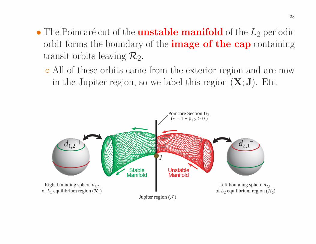
• The Poincare cut of the unstable manifold of the L2 periodicorbit forms the boundary of the image of the cap containingtransit orbits leaving R2.◦ All of these orbits came from the exterior region and are now

in the Jupiter region, so we label this region (X; J). Etc.




J

StableManifold

UnstableManifold


d1,2+ d2,1

−

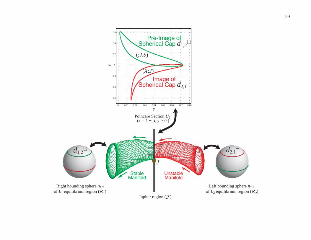
39




0 0.01 0.02 0.04 0.05 0.06 0.07 0.08

-0.6

-0.4

-0.2

0

0.2

0.4

0.6

yy

(;J,S)

(X;J)

Image ofSpherical Cap d2,1

−

J

StableManifold

UnstableManifold

Pre-Image ofSpherical Cap d1,2

+


d1,2+ d2,1

−

0.03

40

◦ The dynamics of the invariant manifold tubes naturally sug-gest the itinerary representation.

∆J = (X;J,S)

Intersection Region

0.92 0.94 0.96 0.98 1 1.02 1.04 1.06 1.08

-0.08

-0.06

-0.04

-0.02

0

0.02

0.04

0.06

0.08

x (rotating frame)

y (r

otat

ing

fram

e)

JL1 L2

Forbidden Region

Forbidden Region

Poincare

section

StableManifold

UnstableManifold

StableManifold Cut

UnstableManifold Cut-0.6

-0.4

-0.2

0

0.2

0.4

0.6

y

(;J,S)

(X;J)

UnstableManifold Cut

StableManifold Cut

(;J,S)

(X;J)

y0 0.01 0.02 0.04 0.05 0.06 0.07 0.08

y0.03

y

41

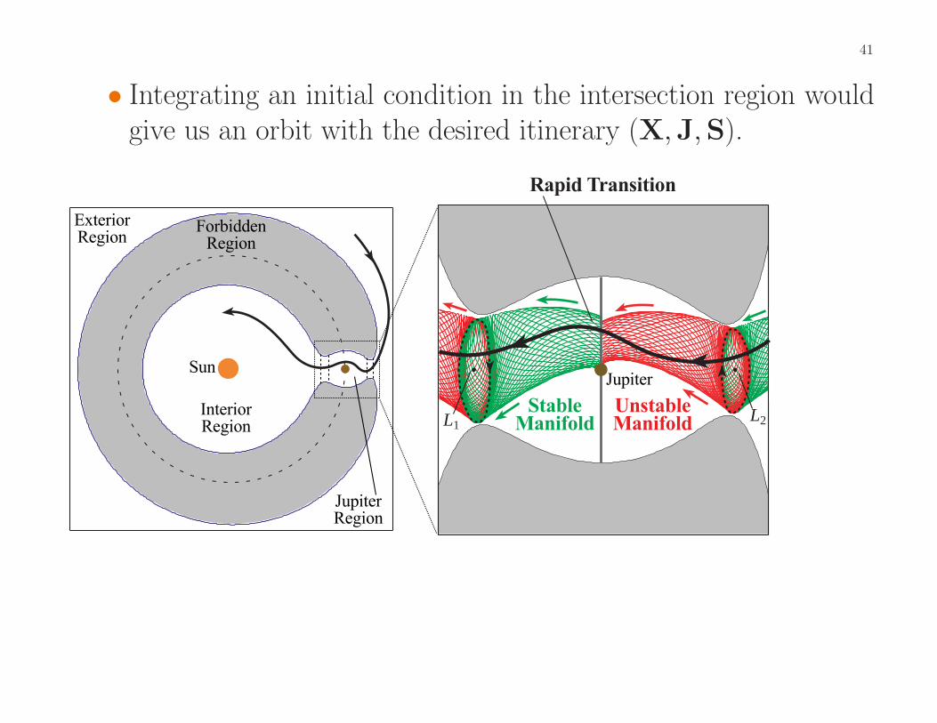
• Integrating an initial condition in the intersection region wouldgive us an orbit with the desired itinerary (X,J,S).

ExteriorRegion

InteriorRegion

JupiterRegion

ForbiddenRegion

L1L2

StableManifold

UnstableManifold

JupiterSun

Rapid Transition

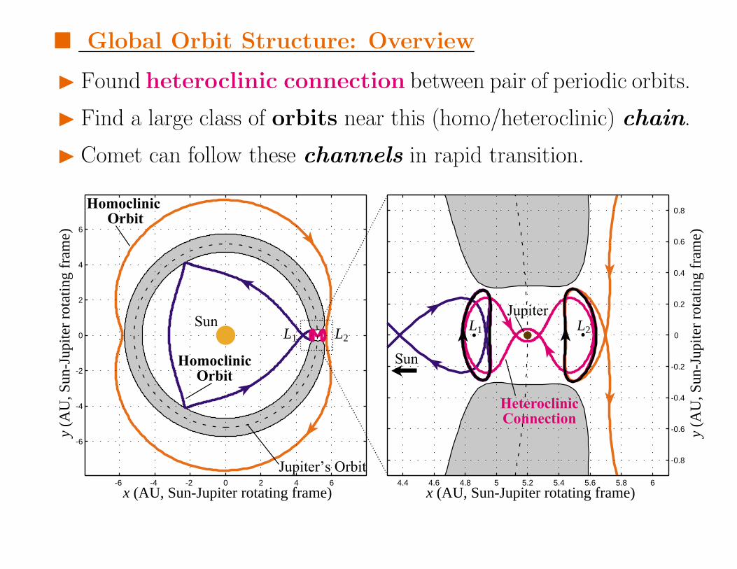
� Global Orbit Structure: Overview

� Found heteroclinic connection between pair of periodic orbits.

� Find a large class of orbits near this (homo/heteroclinic) chain.

� Comet can follow these channels in rapid transition.

-6 -4 -2 0 2 4 6

-6

-4

-2

0

2

4

6

4.4 4.6 4.8 5 5.2 5.4 5.6 5.8 6

-0.8

-0.6

-0.4

-0.2

0

0.2

0.4

0.6

0.8

Sun

Jupiter’s Orbit

x (AU, Sun-Jupiter rotating frame)

y (A

U, S

un-J

upite

r ro

tatin

g fr

ame)


y (A

U, S

un-J

upite

r ro

tatin

g fr

ame)

Jupiter

SunHomoclinicOrbit

Homoclinic Orbit

L1 L2L1 L2


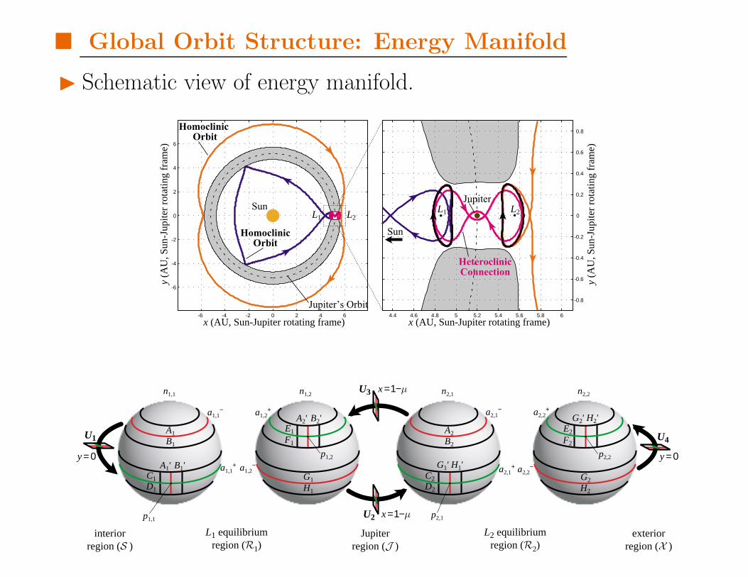
� Global Orbit Structure: Energy Manifold

� Schematic view of energy manifold.

-6 -4 -2 0 2 4 6

-6

-4

-2

0

2

4

6

4.4 4.6 4.8 5 5.2 5.4 5.6 5.8 6

-0.8

-0.6

-0.4

-0.2

0

0.2

0.4

0.6

0.8

Sun

Jupiter’s Orbit


y (A

U, S

un-J

upite

r ro

tatin

g fr

ame)


y (A

U, S

un-J

upite

r ro

tatin

g fr

ame)

Jupiter

SunHomoclinicOrbit

Homoclinic Orbit

L1 L2L1 L2


A1

B1

D1

C1

A1' B1'

E1

F1

H1

G1

A2' B2'A2

B2

D2

C2

G1' H1'

E2

F2

H2

G2

G2' H2'

n1,1 n1,2 n2,1 n2,2

a1,1+

a1,1− a1,2

+

a1,2− a2,1

+

a2,1− a2,2

+

a2,2−

U3

U2

U4U1

interiorregion (S )

exteriorregion (X )

Jupiterregion (J )

L1 equilibriumregion (R1)


p1,1

p1,2

p2,1

p2,2y = 0

x = 1−µ

x = 1−µ

y = 0

� Global Orbit Structure: Poincare Map

� Reducing study of global orbit structure to study of discrete map.

A1

B1

D1

C1

A1' B1'

E1

F1

H1

G1

A2' B2'A2

B2

D2

C2

G1' H1'

E2

F2

H2

G2

G2' H2'

n1,1 n1,2 n2,1 n2,2

a1,1+

a1,1− a1,2

+

a1,2− a2,1

+

a2,1− a2,2

+

a2,2−

U3

U2

U4U1

interiorregion (S )

exteriorregion (X )

Jupiterregion (J )



p1,1

p1,2

p2,1

p2,2y = 0

x = 1−µ

x = 1−µ

y = 0

U3

U2

U4U1interiorregion

exteriorregion

Jupiterregion

A1'

B1'

C1

D1

U1

E1

F1

A2'

B2'

U3

C2

D2

G1'

H1'

U2

E2

F2

G2'

H2'

U4

y = 0

x = 1−µ

x = 1−µ

y = 0

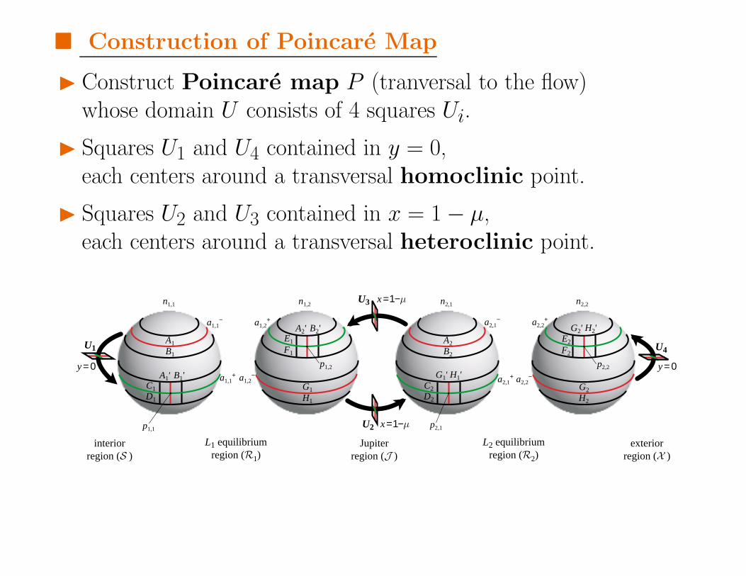
� Construction of Poincare Map

� Construct Poincare map P (tranversal to the flow)whose domain U consists of 4 squares Ui.

� Squares U1 and U4 contained in y = 0,each centers around a transversal homoclinic point.

� Squares U2 and U3 contained in x = 1 − µ,each centers around a transversal heteroclinic point.

A1

B1

D1

C1

A1' B1'

E1

F1

H1

G1

A2' B2'A2

B2

D2

C2

G1' H1'

E2

F2

H2

G2

G2' H2'

n1,1 n1,2 n2,1 n2,2

a1,1+

a1,1− a1,2

+

a1,2− a2,1

+

a2,1− a2,2

+

a2,2−

U3

U2

U4U1

interiorregion (S )

exteriorregion (X )

Jupiterregion (J )



p1,1

p1,2

p2,1

p2,2y = 0

x = 1−µ

x = 1−µ

y = 0

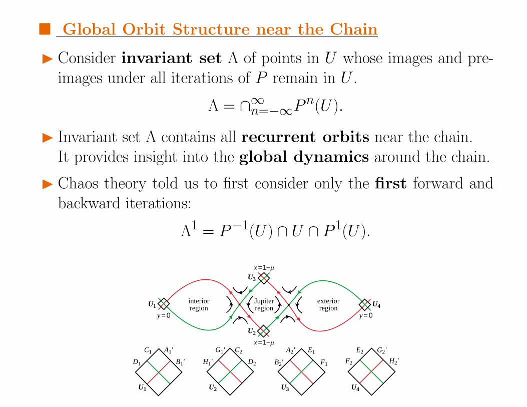
� Global Orbit Structure near the Chain

� Consider invariant set Λ of points in U whose images and pre-images under all iterations of P remain in U .

Λ = ∩∞n=−∞Pn(U).

� Invariant set Λ contains all recurrent orbits near the chain.It provides insight into the global dynamics around the chain.

� Chaos theory told us to first consider only the first forward andbackward iterations:

Λ1 = P−1(U) ∩ U ∩ P 1(U).

U3

U2

U4U1interiorregion

exteriorregion

Jupiterregion

A1'

B1'

C1

D1

U1

E1

F1

A2'

B2'

U3

C2

D2

G1'

H1'

U2

E2

F2

G2'

H2'

U4

y = 0

x = 1−µ

x = 1−µ

y = 0

� Review of Horseshoe Dynamics: Pendulum

� Review of Horseshoe Dynamics: Forced Pendulum

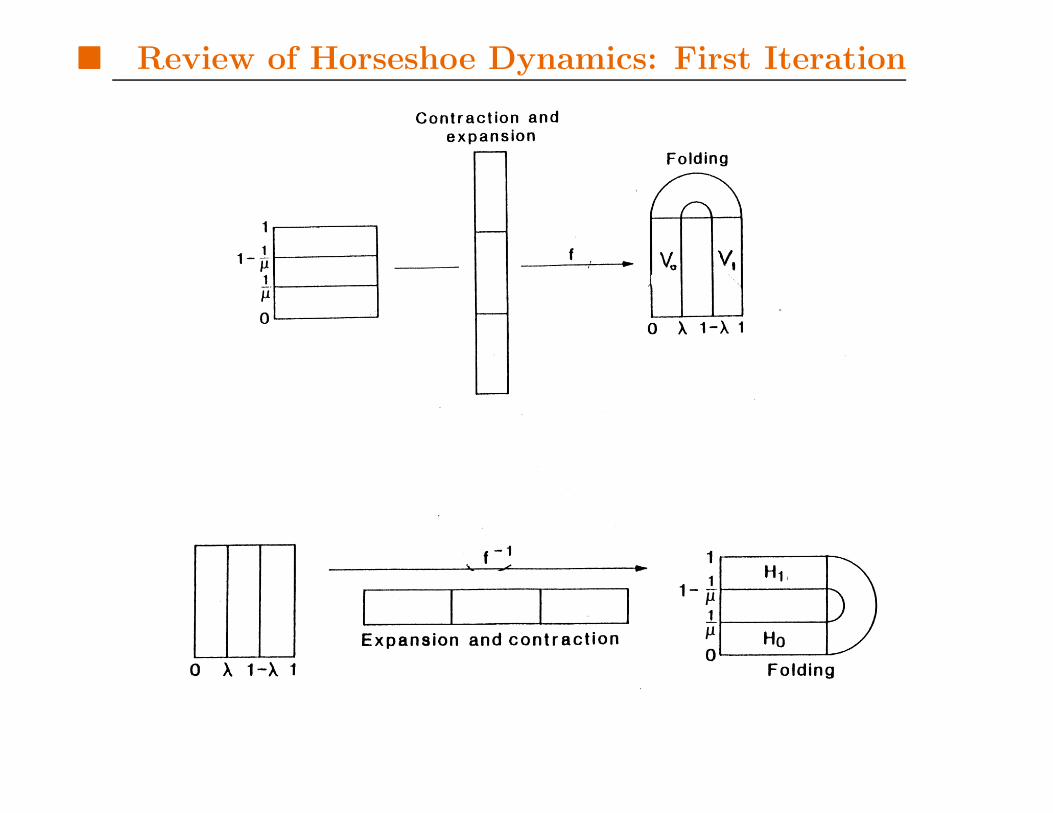
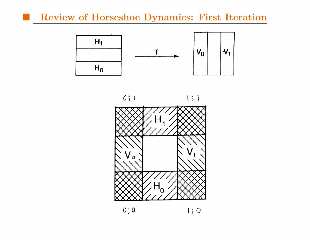
� Review of Horseshoe Dynamics: First Iteration

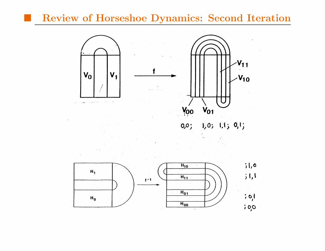
� Review of Horseshoe Dynamics: Second Iteration

� Review of Horseshoe Dynamics: Second Iteration

...0,0; ...1,0; ...1,1; ...0,1;

;1,0...

;1,1...

;0,1...

;0,0...

...1,0;1,1...

D

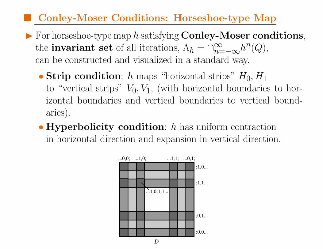
� Conley-Moser Conditions: Horseshoe-type Map

� For horseshoe-type map h satisfying Conley-Moser conditions,the invariant set of all iterations, Λh = ∩∞

n=−∞hn(Q),can be constructed and visualized in a standard way.

• Strip condition: h maps “horizontal strips” H0, H1to “vertical strips” V0, V1, (with horizontal boundaries to hor-izontal boundaries and vertical boundaries to vertical bound-aries).

• Hyperbolicity condition: h has uniform contractionin horizontal direction and expansion in vertical direction.

...0,0; ...1,0; ...1,1; ...0,1;

;1,0...

;1,1...

;0,1...

;0,0...

...1,0;1,1...

D

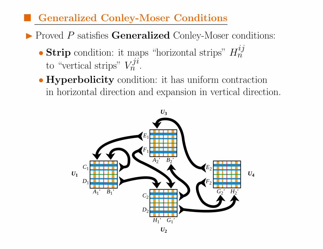
� Generalized Conley-Moser Conditions

� Proved P satisfies Generalized Conley-Moser conditions:

• Strip condition: it maps “horizontal strips” Hijn

to “vertical strips” Vjin .

• Hyperbolicity condition: it has uniform contractionin horizontal direction and expansion in vertical direction.

A1' B1'

C1

D1

U1

U2

H1' G1'

C2

D2

U3

A2' B2'

E1

F1

U4

G2' H2'

E2

F2

� Generalized Conley-Moser Conditions

� Shown are invariant set Λ1 under first iteration.

� Since P satisfies Generalized Conley-Moser Conditions,this process can be repeated ad infinitum.

� What remains is invariant set of points Λ which are in 1-to-1corr. with set of bi-infinite sequences (. . . , ui, m; uj, n, uk, . . . ).

A1' B1'

C1

D1

H2’

Hn11

Hn12

Vm13 Vm

11

C2

D2

C1

D1

A2' B2' A1' B1'

H1' G1'

C2

D2

Hn23

Hn24

Vm21 Vm

23

H2’

A2' B2'

E1

F1

Hn31

Hn32

Vm34 Vm

32

H2’

G2' H2'

E2

F2

Hn43

Hn44

Vm44 Vm

42

U1

U2

U3

U4Qm;n

3;12

� Global Orbit Structure: Main Theorem

� Main Theorem: For any admissible itinerary,e.g., (. . . ,X,1,J,0;S,1,J,2,X, . . . ), there exists an orbit whosewhereabouts matches this itinerary.

� Can even specify number of revolutions the comet makesaround Sun & Jupiter.

S J

L1 L2

X

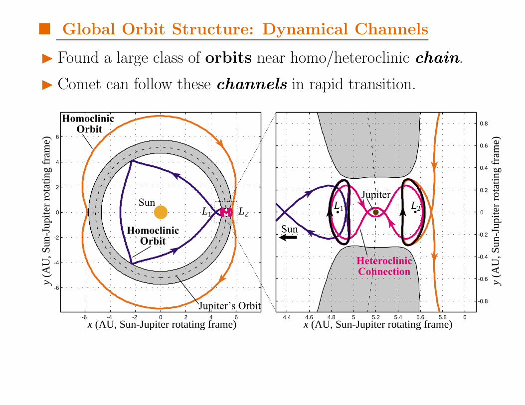
� Global Orbit Structure: Dynamical Channels

� Found a large class of orbits near homo/heteroclinic chain.

� Comet can follow these channels in rapid transition.

-6 -4 -2 0 2 4 6

-6

-4

-2

0

2

4

6

4.4 4.6 4.8 5 5.2 5.4 5.6 5.8 6

-0.8

-0.6

-0.4

-0.2

0

0.2

0.4

0.6

0.8

Sun

Jupiter’s Orbit


y (A

U, S

un-J

upite

r ro

tatin

g fr

ame)


y (A

U, S

un-J

upite

r ro

tatin

g fr

ame)

Jupiter

SunHomoclinicOrbit

Homoclinic Orbit

L1 L2L1 L2


42

Lunar Capture: How to get to the Moon Cheaply

• Using the invariant manifold tubes as the building blocks, wecan construct interesting, fuel saving space mission trajectories.◦ For instance, an Earth-to-Moon ballistic capture orbit.◦ Uses Sun’s perturbation.◦ Jump from Sun-Earth-S/C system to Earth-Moon-S/C sys-

tem.◦ Saves about 20% of onboard fuel compared to Apollo-like

transfer.

43

x

y

L2 orbit

Sun

Lunar Capture

Portion

Earth Targeting Portion

Using "Twisting"

Moon's

Orbit

Earth

L2

Maneuver (∆V)at Patch Point

44

• Intersection found between Earth-Moon stable manifold andSun-Earth unstable manifold, which targets trajectory back toEarth.

xy

L2 orbit

Sun

Lunar Capture

Portion

Earth Backward Targeting

Portion Using "Twisting"

Moon's

Orbit

Earth

L2

0 0.001 0.002 0.003 0.004 0.005 0.006

0.06

0.05

0.04

0.03

0.02

0.01

0

0.01

y(S

un-E

arth

rot

atin

g fr

ame)

.

y (Sun-Earth rotating frame)

Earth-Moon L2Orbit StableManifold Cut

InitialCondition

Sun-Earth L2Orbit

Unstable Manifold CutInitial

Condition

Poincare Section

45

Movie: Shoot the Moon inrotating frame

46

Future Research Directions

• For a single 3-body system:◦When is 3-body effect more important than 2-body?◦ Find “sweet spot” within tubes where transport is most

efficient/fastest?◦ Consider continuous low-thrust control, optimal control.• For coupling multiple 3-body systems:◦Where to jump from one 3-body system to another?◦ Optimal control: trade off between travel time and fuel.◦ Efficient use of resonances• Planetary science/astronomy applications:◦ Statistics: transport rates, capture probabilities, etc.• Chemical/atomic physics applications?

47

• Final Thought: For a class of Hamiltonian systems which havephase space bottlenecks containing unstable periodic orbits, theunstable and stable manifolds of those periodic orbits partition thepart of the energy surface where transport is possible. The mani-folds not only provide a picture of the global behavior of the system,but are the starting point for obtaining the statistical properties ofthe system.

48

Further Information

•Koon, W.S., M.W. Lo, J.E. Marsden and S.D. Ross[2000], Heteroclinic connections between periodic orbits and res-onance transitions in celestial mechanics, Chaos, vol. 10(2), pp.427-469.

•Koon, W.S., M.W. Lo, J.E. Marsden and S.D. Ross[2000], Low energy transfer to the Moon.

• Jaffe, C., D. Farrelly and T. Uzer [1999], Transition statein atomic physics, Phys. Rev. A, vol. 60(5), pp. 3833-3850.

• http://www.cds.caltech.edu/˜shane/

the three-body problemsome interesting dynamics inperiodic

Documents