the theory of(exclusively) local beables
TRANSCRIPT

arX
iv:0
909.
4553
v3 [
quan
t-ph
] 1
7 Ju
n 20
10
The Theory of (Exclusively) Local Beables
Travis Norsen
Marlboro College
Marlboro, VT 05344
(Dated: June 17, 2010)
Abstract
It is shown how, starting with the de Broglie - Bohm pilot-wave theory, one can construct a new theory
of the sort envisioned by several of QM’s founders: a Theory of Exclusively Local Beables (TELB). In
particular, the usual quantum mechanical wave function (a function on a high-dimensional configuration
space) is not among the beables posited by the new theory. Instead, each particle has an associated “pilot-
wave” field (living in physical space). A number of additional fields (also fields on physical space) maintain
what is described, in ordinary quantum theory, as “entanglement.” The theory allows some interesting
new perspective on the kind of causation involved in pilot-wave theories in general. And it provides also
a concrete example of an empirically viable quantum theory in whose formulation the wave function (on
configuration space) does not appear – i.e., it is a theory according to which nothing corresponding to the
configuration space wave function need actually exist. That is the theory’s raison d’etre and perhaps its only
virtue. Its vices include the fact that it only reproduces the empirical predictions of the ordinary pilot-wave
theory (equivalent, of course, to the predictions of ordinary quantum theory) for spinless non-relativistic
particles, and only then for wave functions that are everywhere analytic. The goal is thus not to recommend
the TELB proposed here as a replacement for ordinary pilot-wave theory (or ordinary quantum theory), but
is rather to illustrate (with a crude first stab) that it might be possible to construct a plausible, empirically
viable TELB, and to recommend this as an interesting and perhaps-fruitful program for future research.
1

I. INTRODUCTION
From the very beginning, the quantum revolution centered around the idea of “wave-particle
duality”. Einstein’s revolution-triggering 1905 paper (that is, the one titled “Concerning an heuris-
tic point of view toward the emission and transformation of light”) begins with a discussion of the
“profound formal distinction” between the continuous fields (described by Maxwell’s theory of elec-
tromagnetic processes) and discontinuous particles (exemplified by atoms and electrons) of classical
physics. [1] The need for a novel theory of course arose from the appearance, in certain key ex-
periments, of discontinuous (particle-like) properties in light – and (later) continuous (field-like)
properties in electrons and other material particles.
The obvious and natural way of accounting for such “dual” appearances is simply to take the
duality literally – that is, to say that what we call a “photon” or “electron” actually comprises
two distinct (though inseparable and interacting) entities: a point-like particle, and an associated
wave which somehow guides or choreographs the particle’s motion. Einstein gestured tentatively
toward such a theory of light already in his 1905 paper, and came to endorse such a picture much
more openly (though never fully in publication) in the subsequent decades. Eugene Wigner, for
example, reports that Einstein
“was very early well aware of the wave-particle duality of the behavior of light (and
also of particles); in their propagation they show a wave character and show, in par-
ticular, interference effects. Their emission and absorption are instantaneous, they
behave at these events like particles. In order to explain this duality of their behavior,
Einstein proposed the idea of a ‘guiding field’ (Fuhrungsfeld). This field obeys the
field equations for light, that is Maxwell’s equation. However the field only serves to
guide the light quanta or particles, they move into the regions where the intensity of
the field is high.” [2]
One of Einstein’s early biographers, Philipp Frank, similarly reports that in “conversation Einstein
expressed this dual charater of light as follows: ‘Somewhere in the continuous light waves there are
certain ‘peas’, the light quanta’.” [3]
Given the simplicity and naturalness of this way of understanding the empirical wave-particle
duality, it is not surprising that many other physicists picked up and developed – or independently
arrived at – the same kind of picture. Hendrik Lorentz, for example, still advocated in 1927 (what
de Broglie had dubbed) a “pilot-wave” model of light, and credited the idea to Einstein:
2

“Can the [wave and particle characters of light] be reconciled? I should like to put
forward some considerations about this question, but I must first say that Einstein is to
be given credit for whatever in them may be sound. As I know his ideas concerning the
points to be discussed only by verbal communication, however, and even by hearsay,
I have to take the responsibility for all that remains unsatisfactory.” [4]
Lorentz then goes on to develop a precise – though ultimately untenable – mathematical formulation
of this model.
John Slater reports that, several years earlier, he and many others had also been working on
the same ideas: a
“number of scientists – W.F.G. Swann among others – had suggested that the purpose
of the electromagnetic field was not to carry a continuously distributed density of
energy, but to guide the photons in some manner. This was the point of view which
appealed to me, and during my period at the Cavendish Laboratory in the fall of 1923,
I elaborated it.” [5, 6]
Curiously, though, these early pilot-wave models of light rarely made it into publication, and seem
to have been largely forgotten.
Part of the reason for this is the emergence and ascendancy of the Copenhagen “tranquilizing
philosophy” (as Einstein once called Bohr’s ideology of Complementarity). [7] Slater, for example,
reports that the pilot-wave ontology found no sympathy with Bohr and his colleagues, and was
eventually just lost in the rising tide of the Copenhagen hegemony:
“As soon as I discussed [these ideas] with Bohr and Kramers, I found them enthu-
siastic about the idea of the electromagnetic waves emitted by oscillators during the
stationary states... But to my consternation I found that they completely refused to
admit the real existence of the photons. It had never occurred to me that they would
object to what seemed like so obvious a deduction from many types of experiments.
.... This conflict, in which I acquiesced to their point of view but by no means was
convinced by any arguments they tried to bring up, led to a great coolness between
me and Bohr, which was never completely removed.” [6]
Of course, around this same time, Louis de Broglie had proposed extending the wave-particle
duality – by then a clear empirical fact for light – also to electrons and other material particles.
3

Einstein remarked that de Broglie had thus “lifted a corner of the great veil.” [8, p 43] As Slater
tells it, de Broglie’s
“point of view about the relation of photons and the electromagnetic field was es-
sentially the same one to which I had come practically simultaneously. But he did
not have the antagonism of Bohr to contend with, and consequently he followed his
ideas to their obvious conclusion. If there were an electromagnetic wave to guide the
scattered photon in the Compton effect, why should there not also be a wave of some
sort to guide the recoil electron? The two were inextricably tied together. Thus came
the origin of wave mechanics.” [6]
Wave mechanics reached its culmination in 1926, when Schrodinger developed the dynamical time-
evolution equation for de Broglie’s electron waves. Although Schrodinger himself didn’t favor a
pilot-wave ontology, but instead wanted to invest the wave function alone with physical reality,
several physicists – Einstein, de Broglie, and presumably others – were working during this same
period to construct a full, mathematically-precise pilot-wave theory for electrons. Indeed, Einstein
developed such a theory, which he presented in May of 1927 at a meeting of the Prussian Academy
of Sciences, and which he (it seems) also intended to present at the 1927 Solvay conference. But he
retracted his paper (which was then never published) at the last minute. [9, 10] (See also section
11.3 of Ref. [8].) De Broglie’s pilot-wave theory for electrons was published and subsequently
presented at Solvay in 1927, and was the subject of extensive discussion there. [8]
As is well-known, however, shortly after 1927, the pilot-wave ontology (now for electrons) also
sank into obscurity. This is in no small part due, again, to the rising influence of Bohr and the
Copenhagen approach to quantum theory. [11] De Broglie himself rather tragically abandoned
his own theory, based on some combination of failing to understand fully the implications of his
own ideas, and what seems to have amounted to intense peer pressure. David Bohm, 25 years
later in 1952, independently rediscovered and further developed the pilot-wave approach to (non-
relativistic, many particle) quantum mechanics. [12] But Bohm’s theory too remained outside the
scientific mainstream.
The de Broglie - Bohm theory (a.k.a. “Bohmian Mechanics”) has enjoyed, in recent decades,
renewed attention, triggered largely by the support of J.S. Bell and in particular by the role played
by the pilot-wave theory in stimulating the thinking that led to Bell’s Theorem. But the theory is
still not widely understood, taught, or appreciated by physicists. The philosophical, historical, and
cultural reasons for this rather curious state of affairs (curious, that is, given the naturalness of
4

the pilot-wave approach to understanding the empirical wave-particle duality) has been explored
in Ref. [11].
Of primary interest to us here, however, is a certain more technical issue which seems to have
played an important role in, at least, Einstein’s assessment of his own and de Broglie’s (and later,
Bohm’s) versions of the pilot-wave theory – and which, indeed, continues to feature prominently
in polemics against the pilot-wave ontology.
The issue is this: those (like Slater) who were initially sympathetic to the pilot-wave ontology no
doubt expected that, for a system of N particles moving in three spatial dimensions, the theoretical
description would be of N wave-particle pairs – each pair consisting of a point particle guided in
some way by an associated wave propagating in 3-space. (Presumably there would also exist, in
the general case, dynamical interactions among the wave-particle pairs.)
But Schrodinger’s wave function for such an N -particle system was emphatically not a set of
N (interacting) waves, each propagating in 3-space. It was, rather, a single wave propagating in
the 3N -dimensional configuration space for the system. De Broglie’s 1927 pilot-wave theory simply
inherited this feature: it was a theory of particles being guided through physical 3-space by a wave,
yes, but a very strange and seemingly too-abstract wave which didn’t live in 3-space at all.
J.S. Bell introduced the term “beables” (a deliberate contrast to the vaguely-defined “observ-
ables” which, he thought, played too prominent a role in orthodox, Copenhagen quantum theory)
to name whatever is posited, by a candidate theory, as corresponding directly to something that
is physically real (independent of any “observation”). [14, p 52] He then divides beables into two
categories, local and non-local:
“Local beables are those which are definitely associated with particular space-time
regions. The electric and magnetic fields of classical electromagnetism, E(t, x) and
B(t, x) are again examples, and so are integrals of them over limited space-time regions.
The total energy in all space, on the other hand, may be a beable, but is certainly not
a local one.” [14, p 234-5]
Actually, Bell’s example here leaves something to be desired. In classical electromagnetism, it is
dubious to regard integrals of the fields (or even, for example, the electromagnetic energy density
at a point) as beables. Such quantities certainly in some sense exist (according to the theory),
but they aren’t, in standard readings of the theory at least, supposed to directly describe physical
reality in the same way that the fields themselves do. They are the sorts of things theorists may
be interested in calculating, but not the sorts of things that physical reality itself is (according to
5

the theory) made of. Bell’s example of a non-local beable – “the total energy in all space” – also
doesn’t seem quite right. This is certainly a non-local quantity, in the sense he explains, but it
doesn’t seem plausible to grant it “beable status” [14, p 53] for the theory in question.
Probably the reason for the confusing examples is that Bell is trying to do the impossible:
to give a familiar example of a non-local beable from an intuitively clear, classical theory. But,
arguably, no such objects exist in any such theories.
In any case, the utility of the local vs. non-local beable distinction becomes clear in the context
of quantum theories which include, among the beables, a wave function which lives, not in 3-space,
but
“in a much bigger space, of 3N -dimensions. It makes no sense to ask for the amplitude
or phase or whatever of the wavefunction at a point in ordinary space. It has neither
amplitude nor phase nor anything else until a multitude of points in ordinary three-
space are specified.” [14, p 204]
For any theory in which the wave function has beable status, then, it is necessarily a non-local
beable. And this provides a convenient alternative way to state what is surprising and unfamiliar
about the de Broglie - Bohm pilot-wave theory: in addition to positing local beables (the particles),
the theory also posits a genuinely non-local beable (the configuration space wave function which
pilots them).
Don Howard has argued that this (and/or the intimately related issue Howard dubs “non-
separability”) was Einstein’s primary concern with his own and de Broglie’s 1927 pilot-wave the-
ories. Indeed, the non-local beable character of Schrodinger’s wave function stood out to Einstein
from the very beginning. Here he is, in a letter to Ehrenfest of April 12, 1926, praising Schrodinger’s
wave mechanics in comparison to Heisenberg’s matrix mechanics, but also noting a curious feature
of the former:
“The Born-Heisenberg thing will certainly not be right. It appears not to be possi-
ble to arrange uniquely the correspondence of a matrix function to an ordinary one.
Nevertheless, a mechanical problem is supposed to correspond uniquely to a matrix
problem. On the other hand, Schrodinger has constructed a highly ingenious theory
of quantum states of an entirely different kind, in which he lets the De Broglie waves
play in phase space. The things appear in the Annalen. No such infernal machine,
but a clear idea and – ‘compelling’ in its application.” [13, p 82-3]
6

But, as Howard notes, “Einstein’s enthusiasm was short lived.” On the first of May, he writes to
Lorentz:
“Schrodinger’s conception of the quantum rules makes a great impression on me; it
seems to me to be a bit of reality, however unclear the sense of waves in n-dimensional
q-space remains.” [13, p 83]
And here he is on June 18, in a letter again to Ehrenfest:
“Schrodinger’s works are wonderful – but even so one nevertheless hardly comes closer
to a real understanding. The field in a many-dimensional coordinate space does not
smell like something real.” [13, p 83]
It didn’t take long for his discomfort with this curious aspect of the de Broglie - Schrodinger wave
to turn into a research program – which program would ultimately be incorporated into Einstein’s
infamous and fruitless search for a “unified field theory”. On June 22, Einstein writes to Lorentz:
“The method of Schrodinger seems indeed more correctly conceived than that of
Heisenberg, and yet it is hard to place a function in coordinate space and view it
as an equivalent for a motion. But if one could succeed in doing something similar in
four-dimensional space, then it would be more satisfying.” [13, p 83]
This thought is repeated in an August 21 letter to Sommerfeld:
“Of the new attempts to obtain a deeper formulation of the quantum laws, that by
Schrodinger pleases me most. If only the undulatory fields introduced there could be
transplanted from the n-dimensional coordinate space to the 3 or 4 dimensional!” [13]
And yet again in an August 28 letter to Ehrenfest:
“Schrodinger is, in the beginning, very captivating. But the waves in n-dimensional
coordinate space are indigestible...” [13]
It is clear, then, that the “indigestibility” of a physically real wave on an abstract, high-dimensional
space was a primary roadblock for Einstein’s acceptance of Schrodinger’s wave mechanics. This is
evidently the feature he had in mind when, in a January 11, 1927 letter to Ehrenfest, he described
the “Schrodinger business” as “noncausal and altogether too primitive” and when, on February 16
in a letter to Lorentz, he denied emphatically that the quantum theory could “be the description
of a real process.” [13, p 84]
7
It stands to reason, then, that this same feature of de Broglie’s mature 1927 pilot-wave theory
(which simply incorporates Schrodinger’s configuration space wave function) stands behind Ein-
stein’s (perhaps otherwise surprisingly) cool reaction to that theory – and also his downright cold
reaction to Bohm’s theory 25 years later. [15]
De Broglie himself also seems to have had reservations about this aspect of his theory. Valentini
and Bacciagaluppi summarize him, in his (May 1927) first full published presentation of his pilot-
wave theory, as asserting “that configuration space is ‘purely abstract’, and that a wave propagating
in this space cannot be a physical wave: instead, the physical picture of the system must involve
N waves propagating in 3-space.” [8, p 68] Later, at the 1927 Solvay conference, de Broglie states:
“It appears to us certain that if one wants to physically represent the evolution of a system of N
corpuscles, one must consider the propagation of N waves in space...” [8, p 79] Unlike Einstein,
however, de Broglie (at least at this time) didn’t seem to appreciate the non-trivial character of the
problem. That is, de Broglie seemed to think that it was somehow unproblematic or straightforward
to interpret Schrodinger’s configuration-space wave as some kind of abstract description of the
desired “N waves propagating in 3-space.” [8, p 69-84]
It is not clear what role de Broglie’s eventual realization that this problem was in fact not trivial
at all, might have played in his decision to give up his theory shortly after 1927. It is clear, however
– and perhaps suggestive – that de Broglie began working on this particular issue immediately after
his interest in the pilot-wave ontology was rekindled by Bohm’s work in 1952. See, for example,
Chapter VI of Ref. [16]. See also Ref. [17] for a helpful review of the various attempts by de
Broglie, Vigier, and others in this direction during this period.1
There is reason to think that this issue was a central concern for others (besides Einstein and de
Broglie) as well. As Linda Wessels reports in recounting “Schrodinger’s Route to Wave Mechanics”
“In the case of a single classical particle ψ could be interpreted as a wave function
describing a matter wave. For a system of n classical particles, however, ψ was a func-
tion of 3n spatial coordinates and therefore described a wave in a 3n-dimensional space
that could not be identified with ordinary physical space. To give his theory a wave
interpretation Schrodinger would either have to show how the ψ in 3n-dimensional
1 It should perhaps be noted that these attempts, as reviewed in particular in Section 5 of Ref. [17], seem to berather muddled and unsuccessful. For example, depending on precisely how one interprets the meaning of thesymbol r that appears (for example) in Equation (5.5), this and other Equations are either trivially wrong or valid(but in a way that severely obfuscates the nature and extent of the difficulty). A more careful and extensive reviewof these historical attempts at creating (what is here being called) a TELB – and their relation to the schemeproposed in the current paper – would I think be worthwhile.
8

space determined n waves in 3-dimensional space, or reformulate the theory so that it
would yield directly the required n wave functions. (Eventually each of these escape
routes were to be explored, but neither would prove successful.)” [18, p 333]
Wessels then adds in a footnote, citing a 1962 interview with Carl Eckart conducted by John
Heilbron: “The obvious solution would be to rewrite the equations of wave mechanics so that even
for a system of several ‘particles’, only three-dimensional wave functions would be determined. C.
Eckart has reported that at one time he attempted this and remarked that it was something that
initially ‘everybody’ was trying to do.” (Emphasis added.)
And this concern over the “non-local beable” character of the pilot wave in pilot-wave theory
remains, to this day, a vulnerable point for polemics against the theory and/or the associated
ontology. For example, two recent commentators have noted that
“If only spacetime is real, one would have to figure out a way to write the wave function
as a function of 3-space instead of 3n-space. This would implement de Broglie’s original
interpretation, in which the Ψ-field is conceived of as propagating in physical space.
Although there have been some attempts at doing this, ... none have been completely
successful. In our opinion, if it can be achieved, this is the most desirable option,
although a certain amount of pessimism concerning its chances is probably in order.”
[19]
And even more recently, this point was raised by N. David Mermin in a passing dig at the theory:
advocates of the pilot-wave theory, he suggests, must implausibly give the “3N -dimensional config-
uration space .... just as much physical reality as the rest of us ascribe to ordinary three-dimensional
space.” [20]
Let us summarize the historical background context we have been surveying and then, finally,
state the thesis of the present article. The two central background claims here are that (i) the
pilot-wave picture is a natural and intuitively-appealing way to try to understand the kinds of
phenomena whose explanation has been, from the very beginning, the whole purpose of quantum
theory; but (ii) the pilot-wave theory (in which one evidently must take the wave function as
physically real, as a beable [14, p 128] ) has been hurt – that is, rejected and marginalized – by the
fact that, at least in extant formulations, the wave which does the piloting is a wave not on physical
3-space, but on an abstract 3N -dimensional configuration space, it being (at best) counter-intuitive
to take such an object as physically real.
9

The point of the present article is to show that, after all, it is possible to formulate a pilot-wave
theory of the sort anticipated and then unsuccessfully sought after by Einstein, de Broglie, and
others – that is, a theory in which N particles are guided by N (interacting) fields in 3-space.
Actually, the theory to be proposed here is not precisely of this sort, because (as we will explain)
additional fields (also in 3-space) are involved as well – fields which do not influence the particles
directly, but only indirectly, by exerting direct influence on the pilot-waves. These new fields, as
it turns out, can be understood as necessary precisely to fix the kinds of problems encountered by
Einstein, Bohr-Kramers-Slater, and other early attempts to construct a quantum theory without
non-local beables: such theories lacked what is now called entanglement and so failed to predict,
for example, strict energy and momentum conservation in scattering processes. (See Chapter 9 of
Ref. [8] for a fuller discussion.)
One important feature of the theory to be presented is simply that it shows (by explicit con-
struction) how one can in principle explain entanglement phenomena (which are in some sense the
essence of quantum theory) without positing any such non-local beable as a wave function living on
a high-dimensional space. Unfortunately, what one does need to posit may seem, by comparison,
extravagant to the point of implausibility. So be it. The theory of exclusively local beables (TELB)
put forward here is only intended as an un-serious toy model, to illustrate in principle that the
kind of theory envisioned by (among others) Einstein and de Broglie can, after all, be constructed.
It should thus be considered merely as a possible jumping-off point for those interested in picking
up and developing this long-since- (but, it seems, prematurely-) abandoned idea.
Let us then turn to seeing how this trick can be done.
II. QUALITATIVE OVERVIEW
We begin with the de Broglie - Bohm pilot-wave theory for (spinless) particles. This is a theory
which, as mentioned, contains both local and non-local beables – the particles and pilot-wave,
respectively.
For simplicity and to make certain features more intuitively graspable, we consider the theory
of N = 2 particles which move in a single spatial dimension. Then the configuration space for
the system is two-dimensional. The time-evolution of the wave function is given, as usual, by
Schrodinger’s equation:
i~∂Ψ(x1, x2, t)
∂t= −
~2
2m1
∂2Ψ(x1, x2, t)
∂x21−
~2
2m2
∂2Ψ(x1, x2, t)
∂x22+ V [x1, x2, t] Ψ(x1, x2, t) (1)
10

where m1 and m2 are, respectively, the masses of particles 1 and 2 and V is the potential energy
associated with the configuration (x1, x2) at time t. We also assume, for reasons that will become
obvious, that the wave function is analytic everywhere.
The time-evolution of the particle positionsX1(t) andX2(t) is determined by the gradient, along
the appropriate direction in configuration space, of the phase of Ψ at the actual configuration point:
dXi(t)
dt=
~
mi
Im
(
∇iΨ
Ψ
)
∣
∣
∣
x1=X1(t), x2=X2(t). (2)
The existence, in the theory, of the “actual configuration” – represented by X1(t) and X2(t) –
allows one to define the so-called “conditional wave-function” for each particle. [21] This is, for a
given particle, simply the full, configuration-space wave function evaluated at the actual location
of the other particle. Thus,
ψ1(x, t) ≡ Ψ(x, x2, t)∣
∣
x2=X2(t)(3)
and
ψ2(x, t) ≡ Ψ(x1, x, t)∣
∣
x1=X1(t). (4)
The idea of using such conditional wave functions as part of the ontology of a pilot-wave theory is
not new. [8, p 79-80] This option is usually abandoned, however, based on an argument that an
ontology consisting exclusively of the particle positions and the conditional wave functions, cannot
work. (See, for example, Ref. [2].) Let us review this.
The time-evolution law for each particle position can be written in terms of the associated
conditional wave function as follows:
dXi(t)
dt=
~
mi
Im
(
∂ψi(x, t)/∂x
ψi(x, t)
)
∣
∣
∣
x=Xi(t). (5)
But the time-evolution of the conditional wave functions themselves depends not only on the
structure of those conditional wave functions (and the particle positions), but also on the full,
configuration-space wave function from which the conditional wave functions were extracted. [22]
We illustrate this here with a simple example that will be useful also in later discussions.
Consider a simple scattering experiment (in our impoverished, 2-dimensional configuration space):
particle 1, following a localized wave-packet, is projected toward particle 2, which is at rest (in a
stationary wave packet) near the origin. The two particles have some kind of contact interaction,
e.g., V (x1, x2, t) ∼ δ(x1 − x2). Assume the strength of the interaction is chosen (relative to the
energies and other properties of the two particles) so that the two possible outcomes – particle 1
11

x1
x2
b
b
FIG. 1: A scattering experiment involving two interacting particles in one spatial dimension: particle 1 is
projected toward particle 2, which is initially at rest at the origin. A contact potential between the two
particles (represented by the diagonal grey line in the figure) causes the initial (dark grey) wave packet in
configuration space to split into non-overlapping final packets (represented by the two light grey blobs).
The actual configuration point at the beginning of the experiment is represented by the black dot in the
dark grey blob; the initial conditional wave functions for the two particles are simply the full wave function
evaluated along (respectively) the two dashed lines through the actual configuration point. (And similarly
for the final conditional wave functions.) We suppose that the initial conditions are such that this initial
configuration leads, by the deterministic pilot-wave dynamics, to the final configuration represented by the
other black dot. This corresponds, in 1-D physical space, to particle 1 having suffered a billiard-ball like
collision in which it stops completely and its momentum is transferred to particle 2, which moves off to the
right (in physical space, not configuration space!).
“tunnels” past particle 2 and continues on its way, or particle 1 collides with particle 2 and stops
while particle 2 moves off to the right – are (according to ordinary QM) equally probable.
The dynamical sequence, in the 2-dimensional configuration space, is illustrated in Figure 1.
Here we suppose that the initial particle positions are such as to produce the second possible out-
come: there is a billiard-ball-like collision in which particle 1 is brought to rest and its momentum
is transfered to particle 2, which moves off.
Now the point is that (without changing either the initial particle positions or the initial con-
ditional wave functions) the initial state of the full, configuration-space wave function could have
been changed so as to produce a dramatically different outcome. For example, had the initial state
12

for Ψ involved an appropriate superposition of incoming waves in the configuration space – as
illustrated in Figure 2 – destructive interference would absolutely prohibit the outcome considered
in the first experiment, and would instead ensure that the actual configuration point emerges to
the right in the figure, i.e., that particle 1 simply tunnels through particle 2 and continues its initial
motion to the right.
Comparison of the two examples thus suggests that the particle positions and conditional wave
functions alone cannot be a sufficient ontology for a theory – different things can happen (according
to the full, configuration-space dynamics) even though the initial particle positions and conditional
wave functions are (in the two examples) identical. The comparison also brings out precisely
what aspect is missing from the proposed ontology: the conditional wave functions necessarily
fail to capture information about the structure of the (full, configuration space) wave function
from regions that are “diagonal” from the actual configuration point. Such information will exist
whenever the wave function fails to factorize, i.e., whenever the quantum state is entangled. And
of course – as the above comparison illustrates – such information can be dynamically relevant to
the motion of the particles (and indeed also the evolution of the conditional wave functions). So
any proposed new ontology has to find a way to capture this information if it is going to reproduce
the empirically correct predictions of the configuration space pilot-wave theory for the particle
trajectories.
Before turning to the approach to be advocated, we consider briefly – for contrast and historical
interest – another way one might consider trying to capture the full relevant structure of the wave
function using fields on physical space: instead of using the conditional wave functions for each
particle, one might form, for each particle, an associated wave on physical space by (squaring and)
projecting. For example, one could define a field for particle 1 this way:
η1(x, t) ≡
∫
|Ψ(x, x2, t)|2 dx2 (6)
and similarly for particle 2. This would give, at the beginning of the experiment shown in Figure
1, a wave packet for particle 1 moving toward a stationary wave packet for particle 2. At the end
of the experiment, however, each particle’s η-field would comprise two packets – one moving and
one stationary – corresponding to the two possible final states of motion for each particle.
One might reasonably attempt to interpret the two packets (for a given particle) as indicating
two possible outcomes only one of which is realized (with the fact about which one is realized being
random and – in particular – independently random for each particle). This would seem to provide
a sensible story about what happens during the scattering process, but note that we would then
13

x1
x2
bb
FIG. 2: A similar scattering experiment: the situation is just as before, but now the initial wave function
represents an entangled state for the two particles, leading to a different outcome even though the initial
particle positions and the initial conditional wave functions are the same as before. This illustrates the way
in which the conditional wave functions fail to capture information about the structure of the (configura-
tion space) wave function which is in a “diagonal” direction (in the configuration space) from the actual
configuration point – i.e., the way in which the conditional wave functions fail to capture entanglement.
lose strict energy and momentum conservation: it might turn out, for example, that both particles
end up at rest near the origin after the experiment. Theories of this sort were considered by (at
least) Einstein and Bohr, Kramers, and Slater, but ultimately given up when it was realized that
strict energy/momentum conservation was required by experiment. See Chapter 9 of Ref. [8] for a
more extended discussion. (Note also the intimate connection between the ontology just proposed
and Schrodinger’s own early views, as reviewed and clarified recently in Ref. [23].)
With that (historically important) alternative approach out of the way, let us return to the
approach to be advocated here: using the conditional wave functions as the basis for an ontology
of exclusively local beables, but supplementing the conditional wave functions with some new (local)
beables in order to capture the dynamically-relevant “diagonal” structure of the full, configuration
space wave function.
A possible way of doing this reveals itself as soon as we attempt to extract a time-evolution
law for the conditional wave functions from the (configuration space) Schrodinger equation. Let us
illustrate this using the conditional wave function for particle 1 from above. Using Equation (3),
14

the time-derivative of ψ1(x, t) can be computed as follows:
∂ψ1(x, t)
∂t=∂Ψ(x, x2, t)
∂t
∣
∣
∣
x2=X2(t)+
dX2(t)
dt
∂Ψ(x, x2, t)
∂x2
∣
∣
∣
x2=X2(t). (7)
The derivative in the first term is given by Equation (1), two of the terms on the right hand side
of which can be written in terms of ψ1(x, t) once evaluated at x2 = X2(t). Multiplying through by
i~, we end up with the following Schrodinger-like equation for the time-evolution of ψ1(x, t):
i~∂ψ1(x, t)
∂t= −
~2
2m1
∂2ψ1(x, t)
∂x2+ V [x,X2(t), t] ψ1(x, t) + A + B (8)
where
A = −~2
2m2
∂2Ψ(x, x2, t)
∂x22
∣
∣
∣
x2=X2(t)(9)
and
B = i~dX2(t)
dt
∂Ψ(x, x2, t)
∂x2
∣
∣
∣
x2=X2(t). (10)
The point, of course, is that the terms we have called A and B cannot be written in terms of the
local beables introduced so far (the particle positions and the conditional wave functions).
This could be thought of as an argument that one cannot construct a TELB using the conditional
wave functions. But in fact what the argument shows us is precisely what additional local beables
we need to add to the ontology in order to have a well-defined, closed dynamics. Specifically, we
introduce the new fields
ψ ′
1(x, t) ≡∂Ψ(x, x2, t)
∂x2
∣
∣
∣
x2=X2(t)(11)
and
ψ ′′
1 (x, t) ≡∂2Ψ(x, x2, t)
∂x22
∣
∣
∣
x2=X2(t). (12)
Don’t be fooled by the notation: these are meant to be taken as genuinely new fields, which
certainly cannot be computed or defined in terms of the conditional wave function ψ1(x, t). The
point of introducing them is of course to make the time-evolution law for ψ1(x, t) well-defined in
terms of posited local beables. It now reads:
i~∂ψ1(x, t)
∂t= −
~2
2m1
∂2ψ1(x, t)
∂x2+ V [x,X2(t), t] ψ1(x, t)
−~2
2m2ψ ′′
1 (x, t) + i~dX2(t)
dtψ ′
1(x, t). (13)
15

(One should understand, here and occasionally in what follows, factors like the dX2/dt on the right
hand side as merely a shorthand for the right hand side of Equation (5) with the appropriate value
of i.)
Of course, having introduced these new local beable fields, e.g., ψ ′
1(x, t), we must now define
their time-evolution. But that can be done straightforwardly (if tediously), by simply taking the
time-derivative of the relevant definition, and using again Schrodinger’s equation. One can see that,
for example, the Schrodinger-like equation satisfied by ψ ′
1(x, t) will involve, on the right-hand-side,
terms including
∂3Ψ(x, x2, t)
∂x32|x2=X2(t) (14)
which we incorporate as a new local beable field, ψ ′′′(x, t). And so on.
And of course all of this is happening in parallel also for particle 2 and its associated fields. In
the end, we have a (countable) infinity of fields associated with each particle: a conditional wave
function which (directly) determines the particle’s velocity at each instant, and then a hierarchy
of additional fields which influence the conditional wave function (and one another) and can be
thought of as simply a way to capture or reproduce – by what amounts to simple Taylor expansion
– the information about the structure of the full, configuration space wave function that the
conditional wave functions alone failed to capture.2
We will reflect later on several interesting features of this theory (and/or the slightly modified
version to be considered in Section IV). For now we note just one important feature: despite being a
theory of (i.e., formulated in terms of) exclusively local beables, the theory is manifestly non-local.
For example, the rate of change of ψ1 (at every point in space!) is influenced by the instantaneous
velocity of particle 2 (or, perhaps more accurately, by the imaginary part of the gradient of the
logarithm of particle 2’s pilot-wave field at the location of particle 2). Not surprisingly, similar
dynamical non-localities will appear in the equations defining the time-evolution of the other fields.
This non-local causation is of course essential to the theory’s ability to reproduce the predictions
2 Here we see clearly the importance of having assumed a (configuration space) wave function that is – for all times– everywhere analytic. For a smooth but non-analytic wave function, the Taylor expansions used here will encodea different “entanglement structure” – and hence imply, eventually, different particle trajectories – than the usualformulation of the pilot-wave theory. Thus, the scheme employed here will only reproduce the predictions of theusual pilot-wave theory for the special case of analytic wave functions. The extent to which this is a seriousshortcoming of the current proposal is perhaps debatable. For example, it would be difficult to cite any empiricalevidence that the usual formulation of pilot-wave theory (as opposed to the formulation developed here) makescorrect predictions for situations involving smooth but non-analytic wave functions. And anyway, there will turnout to be several unrelated – and almost certainly more serious – shortcomings, which render the precise assessmentof the seriousness of this particular one rather moot.
16

of ordinary pilot-wave theory, i.e., essential to its ability to be (in light of Bell’s theorem and the
associated experiments) empirically viable. 3
This is admittedly a complicated, ugly, and highly contrived theory. (And although it is straight-
forward to generalize from 2 particles moving in 1 spatial dimension to N particles moving in 3
spatial dimensions, the complexity and ugliness in that more serious context is surely much worse!)
But it nevertheless represents a way of doing what many physicists took to be important but im-
possible, so we believe it is worth taking somewhat seriously – at least to the point of asking how
one could do better. In the following section, we will briefly summarize in a more formal way the
theory’s ontology and its defining equations. A later section will then present some ideas for how
to use the same basic qualitative approach to construct a (marginally) more plausible theory.
III. A COMPLICATED, UGLY, AND HIGHLY CONTRIVED TELB
The previous section explained how a theory of exclusively local beables (TELB) can be con-
structed, “top-down”, by starting with the ordinary pilot-wave theory (with its non-local beable,
a wave function on configuration space). Here, we take the opposite approach to presenting the
theory and simply lay out the theory’s ontology and dynamics. What makes this interesting is, of
course, that the theory to be presented simply does not include anything like the ordinary quantum
mechanical wave function (on configuration space) but is instead formulated exclusively in terms of
local beables. Yet, as the previous section should have made clear, the theory is (by construction)
empirically equivalent to the de Broglie - Bohm pilot wave theory (at least, as noted, for the case
of analytic wave functions) and hence also to ordinary quantum theory. 4
The ontology of the theory (again, for two particles moving in one spatial dimension) is as
follows: each “particle” (in the informal way of speaking) comprises a literal particle (a point
moving with some definite trajectory through physical space), an associated pilot-wave field, and
an infinite set of what might be termed “entanglement fields”. (For the more general case of N
3 Shelly Goldstein (private communication) points out that, in the presence of such dynamical non-localities, thedistinction between local and non-local beables becomes rather fuzzy: one could, for example, take ordinaryBohmian Mechanics and just say that the universal wave function lives at some particular point in 3-space. Thewave function’s choreography of the particle trajectories would then involve dynamical non-locality, but the theorywould be a TELB. Somehow, though, this strikes one as cheating. Probably the underlying intuitions relate to thesuggestion, from the very end of this paper, that we already have – from pre-theoretical interpretations of certainkey experiments – some qualitative sense of what at least some of the local beables ought to be.
4 Actually, the question of empirical equivalency presupposes also some constraints on allowed initial conditions –an issue we intend to gloss over here. We will discuss this important issue in more detail in the following section,where we present a distinct but related theory which might be taken at least a little more seriously.
17

particles, the taxonomy of “entanglement fields” is a little more complicated, but still basically
straightforward.) It is assumed that the image, in the theory, of the familiar material world is
to be found in the particles – that is, somehow, we can see the particles, but the pilot-wave and
entanglement fields are (like the electric and magnetic fields of classical E&M) invisible.
The particles move according to the following law:
dXi(t)
dt=
~
mi
Im
(
∂ψi(x, t)/∂x
ψi(x, t)
)
∣
∣
∣
x=Xi(t)(15)
while the pilot-wave field for particle 1 evolves in time according to:
i~∂ψ1(x, t)
∂t= −
~2
2m1
∂2ψ1(x, t)
∂x2+ V [x,X2(t), t] ψ1(x, t)
−~2
2m2ψ ′′
1 (x, t) + i~dX2(t)
dtψ ′
1(x, t). (16)
Finally, the particle 1 entanglement fields ψ ′
1(x, t), ψ′′
i (x, t), ψ′′′
i (x, t), etc., evolve according to:
i~∂ψ
(n)1 (x, t)
∂t= −
~2
2m1
∂2ψ(n)1 (x, t)
∂x2−
~2
2m2ψ(n+2)1 (x, t)
+i~dX2(t)
dtψ(n+1)1 (x, t) + Pn (17)
where the potential term P is
Pn ≡
n∑
i=0
(
n
i
)
∂iV
∂xi2[x,X2(t), t]ψ
(n−i)1 (x, t). (18)
And of course one has analogous time-evolution equations for the fields associated with particle 2.
This system of equations evidently describes a well-defined, closed dynamical system in the
sense that providing initial conditions for all of the posited beables determines a unique state
for all the beables at all future times. With initial conditions (especially for the “entanglement
fields”) carefully chosen to reproduce the quantum mechanical structure – and in particular with
appropriately random initial positions for the particles – the system will evidently reproduce exactly
the statistical predictions of ordinary quantum theory (at least for analytic configuration-space
wave functions).
It is of course obvious that we have generated this theory by deducing it, in the manner described
in the previous section, from ordinary pilot-wave theory. And as long as one keeps that origin in
mind, it may seem merely like a (pointless and cumbersome) mathematical reformulation of that
theory. In order to appreciate what is interesting about the theory, therefore, one should attempt to
imagine that it (or something like it) could have come about (in, say, 1926 or 1927) from the conflict
between (i) the intuitively-appealing pilot-wave ontology (with the assumption of pilot-waves in
18

physical space) and (ii) the growing realization that something additional would have to be added
to such a theory in order to ensure strict energy-momentum conservation in individual processes
(and other empirically-observable features related to what is now termed “entanglement”).
From this perspective – and to whatever extent one finds this a plausible thing to imagine –
the proposed theory sheds an interesting new light on ordinary quantum theory and in particu-
lar the status of the wave function therein. For one could imagine, after the present theory had
been proposed and tested, mathematical explorations of its structure and predictions revealing the
possibility of a mathematically-equivalent formulation in terms of a single abstract pilot-wave on
configuration space. From this perspective, the (in our world, familiar) configuration space wave
function would be merely a convenient mathematical device, analogous to Hamilton’s principal
function in classical mechanics – an abstract mathematical quantity which perhaps in some situa-
tions makes calculations simpler or more elegant, but which one needn’t take as indicating the real
existence of anything like a physically real field on configuration space.
IV. A MARGINALLY IMPROVED TELB
One of the implausible features of the theory sketched in the previous section is that an in-
credible fine-tuning of initial conditions is required to reproduce the desired quantum mechanical
predictions. In effect, one has to remember that all of the fields have a certain relation to the
configuration space wave function, and choose their initial values on this basis. For example, even
in a situation (like the experiment discussed before and pictured in Figure 1) where there is initially
no entanglement, all of the primed “entanglement fields” from the theory in the previous section
will be (even initially) non-zero and will require the sort of implausibly fine-tuned initial conditions
just mentioned.
A little thought reveals, though, that when there is no entanglement between the particles
the “entanglement fields” defined in the previous section are all simply proportional to the cor-
responding pilot-wave fields. For example, assuming the configuration space wave function has a
non-entangled, product structure
ψ(x1, x2) = α(x1)β(x2) (19)
it follows that the first-order entanglement field for particle 1 is just proportional to ψ1(x) =
α(x)β(X2(t)):
ψ ′
1(x) ≡∂ψ(x, x2)
∂x2
∣
∣
∣
x2=X2(t)= α(x)
∂β(x2)
∂x2
∣
∣
∣
x2=X2(t). (20)
19
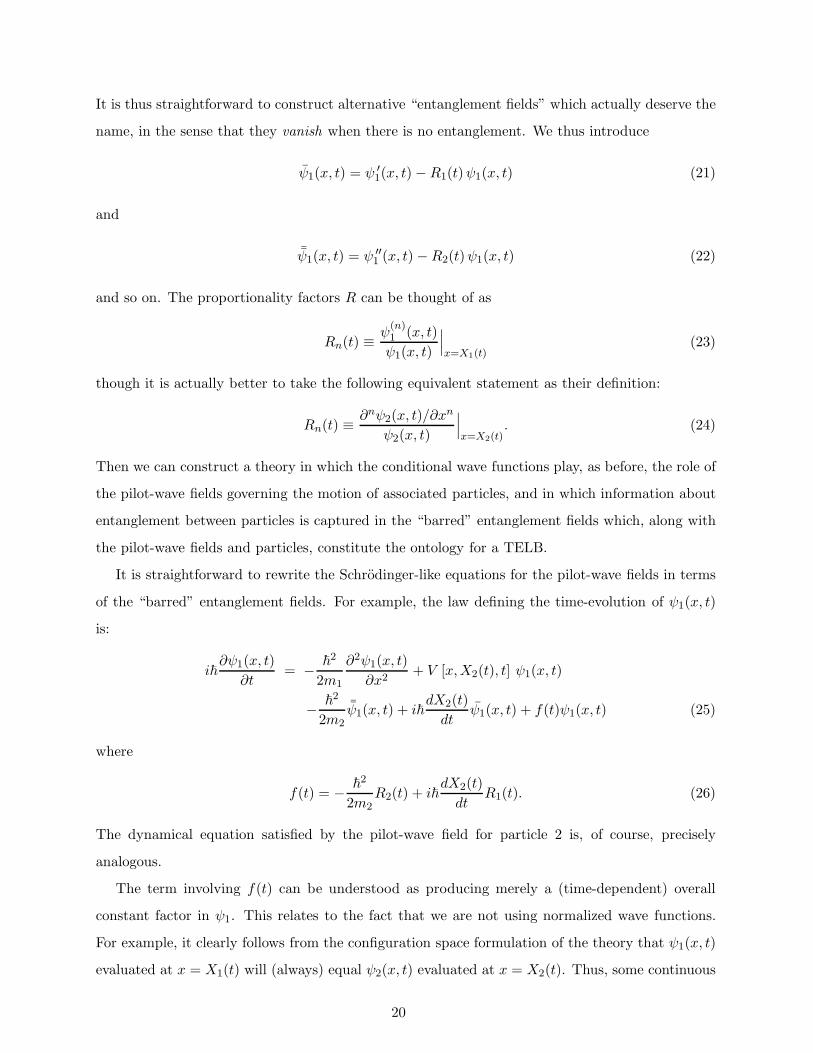
It is thus straightforward to construct alternative “entanglement fields” which actually deserve the
name, in the sense that they vanish when there is no entanglement. We thus introduce
ψ1(x, t) = ψ ′
1(x, t)−R1(t)ψ1(x, t) (21)
and
¯ψ1(x, t) = ψ ′′
1 (x, t)−R2(t)ψ1(x, t) (22)
and so on. The proportionality factors R can be thought of as
Rn(t) ≡ψ(n)1 (x, t)
ψ1(x, t)
∣
∣
∣
x=X1(t)(23)
though it is actually better to take the following equivalent statement as their definition:
Rn(t) ≡∂nψ2(x, t)/∂x
n
ψ2(x, t)
∣
∣
∣
x=X2(t). (24)
Then we can construct a theory in which the conditional wave functions play, as before, the role of
the pilot-wave fields governing the motion of associated particles, and in which information about
entanglement between particles is captured in the “barred” entanglement fields which, along with
the pilot-wave fields and particles, constitute the ontology for a TELB.
It is straightforward to rewrite the Schrodinger-like equations for the pilot-wave fields in terms
of the “barred” entanglement fields. For example, the law defining the time-evolution of ψ1(x, t)
is:
i~∂ψ1(x, t)
∂t= −
~2
2m1
∂2ψ1(x, t)
∂x2+ V [x,X2(t), t] ψ1(x, t)
−~2
2m2
¯ψ1(x, t) + i~dX2(t)
dtψ1(x, t) + f(t)ψ1(x, t) (25)
where
f(t) = −~2
2m2R2(t) + i~
dX2(t)
dtR1(t). (26)
The dynamical equation satisfied by the pilot-wave field for particle 2 is, of course, precisely
analogous.
The term involving f(t) can be understood as producing merely a (time-dependent) overall
constant factor in ψ1. This relates to the fact that we are not using normalized wave functions.
For example, it clearly follows from the configuration space formulation of the theory that ψ1(x, t)
evaluated at x = X1(t) will (always) equal ψ2(x, t) evaluated at x = X2(t). Thus, some continuous
20

re-adjustment of the overall phase and normalization of the pilot-wave fields – unfamiliar from the
point of view of one-particle Schrodinger equations – is clearly necessary here. Of course, one could
eliminate this behavior by using, instead, normalized conditional wave functions as the pilot-wave
fields. This would moderately simplify the Schrodinger-like equations satisfied by those fields, but
would in turn complicate the definition of appropriate entanglement fields. We set this possibility
aside for now.
One can also straightforwardly derive (from the configuration space theory) the time-evolution
equations satisfied by the entanglement fields. For example, ψ1(x, t) will obey the following
Schrodinger-like equation:
i~∂ψ1(x, t)
∂t= −
~2
2m1
∂2ψ1(x, t)
∂x2+ V [x,X2(t), t] ψ1(x, t)
−~2
2m2
(
¯ψ1(x, t)−R1(t)
¯ψ1(x, t))
+ i~dX2(t)
dt
(
¯ψ1(x, t) −R1(t)ψ1(x, t))
+
(
∂V
∂x2[x,X2(t), t]−
∂V
∂x2[X1(t),X2(t), t]
)
ψ1(x, t)
+f(t)ψ1(x, t) (27)
where
f(t) =~2
2m1
∂2ψ1/∂x2
ψ1
∣
∣
∣
x=X1(t)− i~
dX1(t)
dt
∂ψ1/∂x
ψ1
∣
∣
∣
x=X1(t). (28)
The higher-order entanglement fields for particle 1 will obey similar equations (which are straight-
forward to work out), and those for particle 2 are analogous.
Now let’s think about what happens in the scattering experiment discussed earlier (and pictured,
in configuration space, in Figure 1) according to the theory suggested here. At the beginning of
the experiment, there is no entanglement, so all of the (“barred”) entanglement fields vanish
identically – that’s their initial condition. The pilot-wave fields for the two particles will simply be
their ordinary, one-particle wave functions (with the unusual but minor caveat that the amplitude
and phase of the one-particle wave functions should be chosen to respect the condition mentioned
earlier). And the particles themselves should be placed randomly, according to the usual Born
rule prescriptions: P [Xi(0)=x] ∼ |ψi(x, 0)|2. This suffices to define a theory of exclusively local
beables (TELB) which should, like the theory proposed in the previous section, exactly reproduce
the predictions of ordinary pilot-wave theory and hence also ordinary QM, at least for the case
of wave functions which are everywhere analytic. The present re-formulation is an improvement
over that of the previous section because it makes the specification of initial conditions (at least
for situations in which, initially, no entanglement is present) quite natural.
21

The dynamical equations we have presented so far already provide a sufficient basis for under-
standing how things develop in time as the experiment proceeds. To begin with, all the entangle-
ment fields vanish identically, and so the only non-zero terms in Equation (25) will be the familiar
“kinetic energy” and “potential” terms from the usual one-particle Schrodinger equation. (There is
of course also the term, discussed already, which merely changes the overall phase and normaliza-
tion of the pilot-wave field. But this term doesn’t affect the dynamically relevant structure of the
field – i.e., the changes it effects do not influence the motion of the particle being piloted by this
field.) It is also worth mentioning explicitly that the “potential” term involves the “conditional
potential”, i.e., the classical potential field in which particle 1 moves given the actual location of
particle 2. This is, arguably, just what one would expect for the Schrodinger-like equation (for the
pilot-wave) of a single particle, in a pilot-wave TELB.
In any case, it is clear (by thinking about the evolution in configuration space, as indicated in
Figure 1) that entanglement is going to develop when the pilot-wave fields for the two particles
start to overlap in physical space. (Entanglement would develop even earlier if there were long-
range forces between the particles.) We can see how and when this occurs, from the perspective of
the current theory, by examining Equation (27). The only term on the right hand side which can
produce entanglement when there is none to begin with is the term involving ∂V/∂x2 (evaluated at
x2 = X2(t) and then again at the full configuration point) and ψ1(x, t). The factor in parentheses
is like the gradient of the “conditional potential” minus that same quantity evaluated at the actual
location of particle 1. One might call it the “relative conditional potential gradient” – which would
surely not be worth naming in those cumbersome words, if it weren’t for the fact that this quantity
is uniquely responsible for producing (first-order) entanglement between the particles.
For the potential involved in our example – V (x1, x2, t) ∼ δ(x1 − x2) – and given that particle
2 is (at the beginning of the experiment) more or less stationary near the origin, it follows that
the “relative conditional potential gradient” has non-trivial structure (basically, the derivative of
a delta function) also near the origin. So this term comes into play precisely when the incoming
particle 1 wave packet, ψ1(x, t), begins to have support near the origin. This produces (for the first
time) non-zero values for ψ1, which field then acquires a non-trivial dynamical evolution according
to Equation (27). And, of course, the entanglement also feeds back into the dynamical evolution of
the pilot-wave field ψ1(x, t) – and so also the motion of particle 1 – through the appropriate terms
in Equation (25). And of course higher-order entanglement is simultaneously being produced and
feeding back into the dynamics of ψ1 and ψ1. In pattern, it is this production and subsequent
feedback of entanglement which allows our TELB (unlike the earlier TELBs mentioned in the
22

Introduction) to predict strict energy and momentum conservation during the scattering process.
Of course, the main undesirable feature of the theory presented in the previous section is still
with us: a (countably) infinite number of (interacting) fields is still needed to track the dynamics of
the system and reproduce the quantum predictions. We have merely re-organized the information
present in the full configuration space wave function so as to make the specification of initial
conditions more natural; but the same infinite number of fields are still in play.
There is some reason to think, however, that one could achieve sufficiently accurate predictions
by keeping only a finite (and perhaps reasonably small) number of the low-order entanglement fields
for each particle. The basis for this thought is the fact that, at least in the kind of experiment we
have been considering, entanglement is for all practical purposes (FAPP) a transitory phenomenon.
It’s not really transitory, as evidenced by the existence of two widely-separated packets in the
configuration space at the end of the experiment. But it’s FAPP transitory in the sense that
whichever (configuration space) packet fails to contain the actual configuration point, quickly (in
particular, as soon as the packets no longer overlap appreciably) becomes dynamically irrelevant
to the motion of the particles. There is, in the usual language of pilot-wave theory, an “effective
collapse” in the sense that the conditional wave functions acquire (again) the structure of a single
wave packet surrounding the particle and satisfying (again) an ordinary one-particle Schrodinger
equation.
One can understand this, in terms of the theory being developed here, as follows: the en-
tanglement which is present at the end of the experiment is now spread over many high-order
entanglement fields, and manifests as structure in those fields which is far away from the spatial
region where the associated pilot-wave fields have support. It thus affects the pilot-wave fields in
just the same way that they’d be affected by an external potential with non-trivial structure only
where the pilot-wave fields fail to have support – which is to say: it doesn’t affect them at all. The
entanglement, while still in principle present, has become dynamically irrelevant to the evolution
of the pilot-wave fields and hence also the motion of the particles.
Remember, too, that what we are calling the “entanglement fields” can be thought of as captur-
ing (via something like Taylor expansion) the “diagonal” structure of the full configuration space
wave function. And so the thought is: even a finite-order Taylor expansion should do a pretty
fair job of capturing this structure in the immediate vicinity of the point one is expanding around,
which is here the rectangular axes which emerge from the actual configuration point (shown, for
the initial and final moments of the experiment, as the dotted lines in Figure 1).
The lesson is that, at least in this type of phenomenon, the entanglement which is actually
23

relevant to the motion of the particles is transitory and captures information pertaining to regions
of the configuration space wave function that is not too far away (in the configuration space) from
the actual particle configuration. This suggests that we should be able to capture the relevant
entanglement information in a way that is FAPP accurate enough by tracking only a finite (and
not too large) number of the entanglement fields. That is, it suggests that we could truncate the
hierarchy of entanglement fields, keeping only (say) the several lowest-order entanglement fields for
each particle, and still have an empirically adequate theory.
It might be worthwhile to undertake numerical simulations to see what accuracy can be achieved,
for something like the example illustrated in Figure 1, by truncating at different orders. And it
might be worth thinking, in general, about what kinds of situations would most dramatically
distinguish the sort of “truncated TELB” contemplated here with ordinary QM. And it might be
worth studying more carefully the question of whether the dynamics of such a “truncated TELB”
is even mathematically well-defined.
More likely, though, at least at present, such investigations would be simply premature. The
point here is not really to advocate this particular theory. More thinking is needed about how to
best capture the dynamically (most) relevant aspects of the entanglement using fields on physical
space (or other local beables). And more thinking is needed about whether any such theory could
be made to work also in scenarios (such as those involving bound states rather than scattering)
in which dynamically relevant entanglement persists over long periods of time. And there are also
some other reasons (to be discussed shortly) not to take the present theory too seriously. Our goal
here, then, is simply to show that the relevant entanglement information (necessary to reproduce
the strict energy and momentum conservation that was a specific problem for early ideas in the
TELB direction) can, in fact, be captured by local beables – and to suggest that, in principle, a
“reasonable” number of additional fields (or other local beables) might be sufficient to reproduce,
with FAPP sufficient accuracy, the predictions of ordinary quantum theory.
V. DISCUSSION
We have shown that, in principle, it is not hard to construct – starting from extant formulations
of pilot-wave theory involving the configuration space wave function as a non-local beable – a theory
of exclusively local beables (TELB). The sort of theory we have suggested is not precisely of the sort
envisioned by many of QM’s founders (that is, a theory in which the usual wave function on 3N -
dimensional space is replaced by N fields on 3-dimensional space). Instead, this naively-expected
24

ontology forms a foundation on which the full ontology of the new theory is built: it contains
N particles and N pilot-wave fields on physical space, but includes also a number of additional
fields (also on physical space) which capture what is described in ordinary QM as “entanglement”
between particles.
In principle, at least with the kind of scheme explored here, it seems that a (countably) infinite
number of these additional fields is required to precisely reproduce the predictions of ordinary
QM. But as suggested in Section IV there is some reason to think that, for practical purposes, a
finite number of such fields could suffice for empirical adequacy. Of course, this way of putting the
point makes it sound like the purpose of the new theory is merely to replace ordinary QM with an
alternative, in some ways simpler (and for all practical purposes accurate enough) computational
algorithm. The perspective to be considered, though, is just the opposite: the world might include
just a finite number of these entanglement fields, in which case some “truncated pilot-wave theory
of exclusively local beables” like that sketched in the previous section would describe reality ex-
actly, and it would be the ordinary quantum theory (with its configuration space wave function)
which would be merely a convenient computational algorithm, accurate enough for most practical
purposes.
It is interesting to briefly consider the kinds of causation that are present in, say, the theory we
sketched in Section IV. It is clear, first of all, that each particle is “piloted” by its associated pilot-
wave field. In turn, the evolution of a given pilot-wave field is determined by: (i) the structure
of that field itself, as in the usual, one-particle Schrodinger evolution; (ii) the structure of the
associated “entanglement fields” from one and two orders up; and (iii) facts which in some way
pertain to the precise position and/or motion of the other particle. Included in (iii) are several of
the terms on the right hand side of Equation (25) which involve, for example, the instantaneous
velocity of particle 2 and/or facts about the structure of particle 2’s pilot-wave field in the immediate
vicinity of particle 2. And of course the potential energy function (which acts like the potential
energy term in the usual, one-particle Schrodinger equation) is in fact the “conditional potential”,
i.e., the potential field in which particle 1 moves given the actual location of particle 2.
It is sometimes raised as an objection against pilot-wave theory that, in the theory, the wave
function causally influences the particles, but the particles exert no influences back on the wave. [26]
(This, it is apparently thought, suggests that the particles are some kind of mere epiphenomenon,
which might as well be dropped – a bizarre suggestion, for anyone who understands the crucial
role the particles play in making the theory empirically adequate, but still a suggestion one hears
sometimes.) To whatever extent one takes such an objection seriously, then, it is of interest to
25

point out its inapplicability to the pilot-wave theory (of exclusively local beables) sketched here:
each particle’s motion is dictated just by its own associated pilot-wave field, but the evolution
of each pilot-wave field is influenced by all the other particles. Not only, then, do the particles
influence the pilot-wave fields, but the particles can quite reasonably be understood as (indirectly)
affecting each other (through the various fields). Perhaps those who dislike the causality posited
by the usual pilot-wave theory, then, will find the theory sketched here more tolerable.
In elaborating the theory here, we have focused almost exclusively on the case of two spinless,
non-relativistic particles moving in a single spatial dimension. As mentioned already, it is rela-
tively straightforward to generalize everything we’ve done to the case of N spinless non-relativistic
particles moving in 3-space. Incorporating spin is definitely a more serious problem for the specific
theory outlined here, because there is no sensible way to define conditional wave functions for
systems of particles with spin. [21] One might contemplate, instead of incorporating spin through
the wave function as this is done in the currently-standard formulations of the de Broglie - Bohm
theory, introducing spin as a genuine property of particles along the lines of the “rigid rotator”
model presented by Holland [27]; this would seem to allow sensible conditional wave functions for
systems of spinning particles, but at a high price in terms of elegance. Probably a better approach
is to step back and consider alternatives to using the conditional wave functions as the “pilot-wave
fields.” The “conditional quantum potential” and the “conditional velocity field” would seem to
be sensible candidates here since these, like the conditional wave functions, could be thought of
as local beables (in terms of which the motion of the associated particles can be easily specified).
The “conditional density matrices” discussed in Ref. [22] might also be worth considering here.
Considerations of relativistic generalization seem to push in a similar direction. Already in the
case of Galilean boosts in the non-relativistic theory, one has evidence that the conditional wave
functions cannot be taken as the sort of “physical scalar fields” our mathematical formulation makes
them look like. [24] Of course, one could still treat the conditional wave functions as scalar fields if
one abandoned even Galilean relativity and adopted an “Aristotelian” space-time framework. [28]
But it seems much more natural, and much more likely to lead to sensible generalizations in terms
of both spin and relativity, to consider alternative pilot-wave fields (such as those mentioned in the
previous paragraph) as the basis for a pilot-wave TELB.
Finally, we mention again the role of random initial conditions and the emergence of Born rule
probabilities for experimental outcomes. We have suggested that one might be able to increase the
simplicity and plausibility of a theory of exclusively local beables by simply eliminating the high-
order “entanglement fields” – as in the “truncated” theory contemplated in the previous section.
26

Such a maneuvre, while clearly simplifying the theory of exclusively local beables, would instead,
from the point of view of a mathematically equivalent configuration-space theory, complicate things
tremendously! That is, the configuration-space wave function (which would exactly reproduce
the particle trajectories predicted by our truncated TELB) would evidently obey some kind of
complicated, non-linear dynamics, and many of the important mathematical properties of the
usual pilot-wave theory (such as “equivariance” [21]) would no longer hold. From the point of
view of Bohmian Mechanics, it might therefore be hard to see how the “truncated theory of local
beables” could be any kind of positive step – indeed, how such a theory could genuinely be claimed
to make empirically adequate (approximately Born rule) predictions at all.
Here we simply suggest a possible answer. The non-linearities contained in a configuration-space
theory (mathematically equivalent to a “truncated theory of exclusively local beables”) would be,
in principle, similar to the modifications (to standard pilot-wave theory) contemplated by (for
example) Bohm and Vigier, which were believed to drive systems toward Born rule probability
distributions as a kind of dynamical equilibrium. [25] Indeed, it seems that Born rule probability
distributions do emerge naturally at a course-grained level even within the context of the standard,
linear pilot-wave dynamics. [29] This suggests that practically any “small” change to the linear
dynamics (such as that contemplated in the truncated TELBs) might naturally produce Born rule
equilibrium distributions.
If a somewhat more plausible TELB can be constructed (along the lines of the truncated theory
sketched in Section IV, or a new theory with one of the alternative ontologies suggested several
paragraphs back, or something wholly new) it would be quite interesting to investigate in a more
careful way the nature and extent of the differences in empirical predictions between standard
QM and the candidate TELB. Such differences might arise from actual dynamical inequivalencies
(such as those entailed by the truncation scheme suggested earlier), or inequivalencies pertaining in
some way to the implementation or implications of random initial conditions, or from issues arising
from the attempt to develop a TELB which reproduces the predictions of ordinary QM even for
non-analytic wave functions, or from some other novel factor not anticipated here.
For purposes of the present paper, though, our goal is merely to identify the existence of a
large tract of interesting but as-yet completely uncharted theoretical territory – not actually to
start charting it in any serious way. The actual charting will be left for future research, which it is
hoped this paper will help stimulate.
We close with a final remark about “interpreting quantum theory” and the attempt to discover
the real nature of physical systems. The earliest period in the development of quantum theory (from
27

Einstein’s paper in 1905 until, say, de Broglie’s mature pilot-wave theory of 1927) was relatively
healthy from a philosophical point of view. But the subsequent period (after the ascendancy of
Bohr’s Copenhagen approach) had, in retrospect, some clearly unscientific elements and was indeed
detrimental to the ultimate project of understanding the real world (however practical it might
have been in some proscribed, short-term sense to focus on calculations and temporariliy leave
questions of ontology aside). Largely due to the positive influences of J.S. Bell, the community
seems to be recovering from its positivistic ways. To be sure it is still a minority of physicists who
think, for example, that it is important to worry about which realist “interpretation of quantum
theory” might be correct – though the mere existence of such a (growing) minority itself represents
a major turn-around in recent decades.
Unfortunately, though, the most dominant approach to trying to uncover the reality behind
quantum mechanics, is to let the theory itself tell us – as people sometimes say, to simply “read the
correct ontology off” from the equations of the theory. This approach explains (and its dominance
is best established by) the popularity of so-called “many worlds” versions of quantum mechanics,
in which the wave function itself – evolving always according to the unitary Schrodinger equation
– is taken as a complete description of physical reality.
We would like to suggest that this approach is completely flawed, and in fact quite misleading.
One of the lessons of the current work is that mathematically equivalent formulations can have
radically different implications in regard to ontology and causality. (The theory presented in
Section III contains an infinite number of interacting fields on physical space and causal influences
from particles onto the fields associated with other particles – but is mathematically equivalent to
standard pilot-wave theory in which there is just one wave, on configuration space, and no causation
from the particles onto the pilot-wave.) So it seems quite naive to think that one is going to learn
anything useful about external reality by staring at some one particular mathematical formulation
of a theory, and “reading off” an ontology in the most straightforward, naive possible way.
On what, then, should we base our beliefs about the true ontology of the external world? And
what is the proper relationship between ontology and mathematically-formulated physical theories?
Looking at the history of physics suggests an answer. For example, people didn’t come to believe
in the real existence of electric and magnetic fields because vector-valued functions on 3-space were
present in Maxwell’s equations. Rather, the belief in a field ontology came first (via Faraday), and
it was only because this ontology was, at least in a qualitative way, settled, that Maxwell was able
even to conceive the project of working out the detailed mathematical laws for the time-evolution
of those fields.
28
This same pattern seems to play itself out repeatedly in the history of physics: one tries to work
out the correct ontology, the correct slate of beables, first – by making abductive inferences from
the qualitative behaviors observed in certain key experiments – and then one worries about how
to formulate/infer the mathematical laws governing the behavior of those beables.
This is the approach taken by the early developers of quantum theory discussed in the Intro-
duction. It is, for example, quite explicit in one of the remarks of John Slater quoted earlier. And
already in his 1905 paper, Einstein is citing certain key experiments as the basis for the (tentatively)
proposed pilot-wave ontology:
“It seems to me that the observations associated with blackbody radiation, fluores-
cence, the production of cathode rays by ultraviolet light, and other related phenomena
connected with the emission or transformation of light are more readily understood if
one assumes that the energy of light is discontinuously distributed in space.” [1]
Keeping this approach in mind helps one appreciate the fundamental virtue of the pilot-wave
approach. It’s not that pilot-wave theory solves the measurement problem (though it does, and this
is important), nor that the pilot-wave theory allows one to dispense with the usual “measurement
axioms” of orthodox QM and (probably) derive the Born rule (though it does these, too, and these,
too, are important). It’s rather that the pilot-wave theory provides far and away the simplest, most
natural, and most plausible way of understanding all of the key experiments which motivated the
creation of quantum theory in the first place. Einstein and all the other early founders of the
theory perceived this clearly. J.S. Bell, I think, tried to remind us of it when he wrote:
“While the founding fathers agonized over the question
‘particle’ or ‘wave’
de Broglie in 1925 proposed the obvious answer
‘particle’ and ‘wave’.
Is it not clear from the smallness of the scintillation on the screen that we have to do
with a particle? And is it not clear, from the diffraction and interference patterns,
that the motion of the particle is directed by a wave? De Broglie showed in detail how
the motion of a particle, passing through just one of two holes in a screen, could be
29

influenced by waves propagating through both holes. And so influenced that the par-
ticle does not go where the waves cancel out, but is attracted to where they cooperate.
This idea seems to me so natural and simple, to resolve the wave-particle dilemma in
such a clear and ordinary way, that it is a great mystery to me that it was so generally
ignored.” [14, p 191]
While agreeing entirely with Bell here, we also think it is appropriate to concede that there was at
least one puzzling feature of de Broglie’s proposal: the wave, whose real existence is supposed to
have been inferred from the patterns particles make in 3-space, doesn’t itself live in 3-space. So in
a way de Broglie’s theory turned out not to be about what he intended for it to be about.
This, we have suggested, was probably the root of (at least) Einstein’s dissatisfaction not only
with de Broglie’s theory (and later Bohm’s), but the whole “Schrodinger business” – i.e., all of
quantum theory. We have shown, though, that there is actually no significant roadblock in the
way of the kind of theory Einstein (and others) wanted, i.e., a theory whose ontology matches
(or at least includes) the beables one can apparently read off from phenomena like the two-slit
experiment. In fact, there seems to be an abundance of such theories to consider, develop, and
perhaps empirically test.
It is hoped that the ideas presented here will help remind people of this apparently long-
forgotten, but prematurely-abandoned, approach to understanding quantum theory and the world
it describes.
Acknowledgements:
Thanks to Shelly Goldstein, Daniel Victor Tausk, Rob Spekkens, Eric Dennis, and two anony-
mous referees for helpful comments – and in particular for a number of very good, constructively
critical questions, many of which remain insufficiently answered.
[1] Albert Einstein, “Concerning an Heuristic Point of View Toward the Emission and Transformation of
Light”, A.B. Arons and M.B. Peppard, trans., American Journal of Physics, Vol. 33, No. 5, May 1965,
pp 367-374
[2] Eugene P. Wigner, “Thirty Years of Knowing Einstein”, in Some Strangeness in the Proportion, Harry
Woolf, ed., Addison-Wesley, Reading, Massachusetts, 1980
30

[3] Philipp Frank, Einstein: His Life and Times, George Rosen, trans., Alfred A Knopf, New York, 1963,
p 208
[4] H. A. Lorentz, Problems of Modern Physics, Dover Publications, New York, 1967 (a republication of
the work originally published by Ginn and Company in 1927), pp 156-157
[5] See, for example, the note “Radiation and Atoms” in Nature, March 1, 1924, pp 307-8.
[6] John C. Slater, Solid-State and Molecular Theory: A Scientific Biography, John Wiley and Sons, New
York, 1975, pp. 8-14.
[7] K. Przibam, ed., Letters on Wave Mechanics, New York: The Philosophical Library, 1967, p. 31
[8] Antony Valentini and Guido Bacciagaluppi, Quantum Theory at the Crossroads, Cambridge University
Press, 2009 (quant-ph/060918)
[9] Darrin W. Belousek, “Einstein’s 1927 Unpublished Hidden-Variable Theory: Its Background, Context
and Significance”, Stud. Hist. Phil. Mod. Phys. Vol. 27, No. 4, pp. 437-461, 1996
[10] Peter Holland, “What’s wrong with Einstein’s 1927 hidden variable interpretation of quantum mechan-
ics?” Foundations of Physics, 35, 177-96 (2005)
[11] James Cushing, Quantum Mechanics: Historical Contingency and the Copenhagen Hegemony, Univer-
sity of Chicago Press, 1994
[12] David Bohm, “A suggested interpretation of the quantum theory in terms of ‘hidden variables’,” Phys.
Rev., 85 (1952) pp. 166-93
[13] Don Howard, “ ‘Nicht Sein Kann Was Nicht Sein Darf,’ or the Prehistory of EPR, 1909-1935: Einstein’s
Early Worries about the Quantum Mechanics of Composite Systems,” in A.I. Miller, ed., Sixty-Two
Years of Uncertainty, Plenum Press, New York, 1990
[14] J.S. Bell, Speakable and Unspeakable in Quantum Theory, Second Edition, Cambridge University Press,
2004
[15] Here is Einstein, writing to Born in 1952: “Have you noticed that Bohm believes (as de Broglie did, by
the way, 25 years ago) that he is able to interpret the quantum theory in deterministic terms? That
way seems too cheap to me.” Born comments about this: “Although this theory was quite in line with
[Einstein’s] own ideas, to interpret the quantum mechanical formulae in a simple, deterministic way
seemed to him to be ‘too cheap’. Today one hardly ever hears about this attempt of Bohm’s, or similar
ones by de Broglie.” From the perspective being advocated here, it seems that Born has misinterpreted
Einstein’s remark. Einstein is not expressing skepticism about the general project of “interpret[ing] the
quantum theory in deterministic terms” but is instead expressing skepticism about the particular way
this was done by Bohm (and, earlier, de Broglie). Why is the de Broglie - Bohm “way .... too cheap”?
Because it fixes what was, for Einstein, a minor problem (God’s dice-playing), while leaving the major
problem (the presence in the theory of a non-local beable, the wave function on a high-dimensional
space) totally unresolved. Einstein’s letter and Born’s commentary can be found on pages 192-3 of The
Born-Einstein Letters, Irene Born, trans., Walker and Company, New York, 1971.
[16] Louis de Broglie, The Current Interpretation of Wave Mechanics: A Critical Study, Elsevier, Amster-
31

dam, 1964
[17] H. Freistadt, “The Causal Formulation of Quantum Mechanics of Particles (the Theory of De Broglie,
Bohm and Takabayasi)”, Nuovo Cimento, Vol. 5, Supplement 1 (1957) pp. 1-70.
[18] Linda Wessels, “Schrodinger’s Route to Wave Mechanics”, Studies in History and Philosophy of Science
Part A, 10(4), December 1979, pp. 311-340. The remark of Eckart is sourced to a May 31, 1962 interview
with Eckart conducted by J. Heilbron, under the auspices of the AHQP.
[19] Craig Callender and Robert Weingard, “Trouble in Paradise? Problems for Bohm’s Theory”, The
Monist, vol. 80, no. 1 (1997) pp. 24-43
[20] N. David Mermin, “What’s bad about this habit?” Physics Today, May 2009, pp. 8-9.
[21] Detlef Durr, Sheldon Goldstein, and Nino Zanghi, “Quantum Equilibrium and the Origin of Absolute
Uncertainty”, J. Stat. Phys., 67, 843-907 (1992)
[22] Detlef Durr, Sheldon Goldstein, Roderich Tumulka, and Nino Zanghi, “On the Role of Density Matrices
in Bohmian Mechanics”, Foundations of Physics, 35(3), 449-467 (2005)
[23] Valia Allori, Sheldon Goldstein, Roderich Tumulka, and Nino Zanghi, “Many-Worlds and Schroedinger’s
First Quantum Theory”, arxiv 0903.2211
[24] Tim Maudlin, “Completeness, supervenience, and ontology”, J. Phys. A, 40 (2007) 3151-3171.
[25] David Bohm and J.P. Vigier, “Model of the Causal Interpretation of Quantum Theory in Terms of a
Fluid with Irregular Fluctuations”, Phys. Rev., 96, 208-216 (1954)
[26] J. Anandan and H.R. Brown, “On the Reality of Spacetime Geometry and the Wavefunction”, Foun-
dations of Physics, 25 (1995), no. 2, 349
[27] Peter Holland, The Quantum Theory of Motion, Cambridge University Press, 1993
[28] Antony Valentini, “On Galilean and Lorentz invariance in pilot-wave dynamics,” Phys. Lett. A 228
(1997) 215-222.
[29] Antony Valentini and Hans Westman, “Dynamical Origin of Quantum Probabilities”, Proc. Roy. Soc.
London, A461, 253-272 (2005)
32