the theoretical background of factsage - crct

The theoretical background of

GTT-Technologies

The theoretical background of FactSage

The following slides give an abridged overviewof the major underlying principlesof the calculational modulesof FactSage.

GTT-Technologies

Table of Contents

1 Gibbs energy tree and Maxwell relations2 Properties derived from G3 Reaction equilibria and the Law of Mass Action4 Electro-chemical cells5 Complex Equilibria6 From G(T,P,ni) to Phase Diagrams7 Choice of Axes and Types of Phase Diagrams

Note: Click on the icon to return to ToC.

GTT-Technologies

The Gibbs Energy Tree

Mathematical methods are used to derive more information from the Gibbs energy ( of phase(s)or whole systems )

GibbsEnergy

Minimisation

Gibbs-Duhem

Legendre Transform.Partial Derivativeswith Respect tox, T or P

Equilibria

Phase DiagramMaxwellH, U, F µi,cp(i),H(i),S(i),ai,vi

Mathematical Method

Calculational result derived

from G

Page 1.1

GTT-Technologies

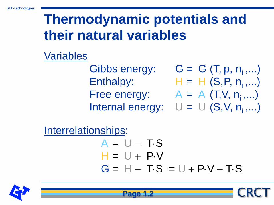
Thermodynamic potentials and their natural variablesVariables

Gibbs energy: G = G (T, p, ni ,...) Enthalpy: H = H (S,P, ni ,...) Free energy: A = A (T,V, ni ,...) Internal energy: U = U (S,V, ni ,...)

Interrelationships:A = U − T⋅SH = U + P⋅VG = H − T⋅S = U + P⋅V − T⋅S

Page 1.2

GTT-Technologies

PTii n

Gµ,

∂∂

=VTin

A

,

∂∂

=PSin

H

,

∂∂

=VSin

U

,

∂∂

=

Maxwell-relations:

Thermodynamic potentials and their natural variables

VPH=

∂∂

STG

−=∂∂

PP TT

S U V

H A

G

S V

and

Page 1.3

GTT-Technologies

...nV,S,const.for0 i,

==

dUU min

...np,T,const.for0 i,

==

dGG min

Thermodynamic potentials and their naturalEquilibrium condition:

...nU,T,const.for0 i,

==

dTA min

...np,S,const.for0 i,

==

dHH min

...nV,U,const.for0 i,

==

dSS max

Page 1.4

GTT-Technologies

Temperature

Composition

ii

i

i

npnpp

np

np

TGT

THc

TGTGSTGH

TGS

,2

2

,

,

,

∂∂

−=

∂∂

=

∂∂

−=+=

∂∂

−=

Use of model equations permits to start at either end!

Gibbs-Duhem integrationPartial Operator

Integral quantity: G, H, S, cp

Partial quantity: µi, hi, si, cp(i)

Thermodynamic propertiesfrom the Gibbs-energy

Page 2.1

GTT-Technologies

With (G is an extensive property!)

one obtains

T,pinG

i

∂∂

=µJ.W. Gibbs defined the chemical potential of a component as:

( ) mi GnG ∑=


( )

( ) mi

im

mii

i

Gn

nG

Gnn

∂∂

+=

∂∂

=

∑

∑µ

Page 2.2

GTT-Technologies

Transformation to mole fractions :

mi

imi

mi Gx

xGx

G∂∂

−∂∂

+= ∑µi

ii x

xx ∂

∂−

∂∂

+ ∑1 = partial operator

ii xn →


mpCipc

mpCmpC

mi

imi

mi Hx

xHx

Hh∂∂

−∂∂

+= ∑

mSis mS mS

Page 2.3

GTT-Technologies

Gibbs energy functionfor a pure substance• G(T) (i.e. neglecting pressure terms) is calculated from the

enthalpy H(T) and the entropy S(T) using the well-knownGibbs-Helmholtz relation:

• In this H(T) is

• and S(T) is

• Thus for a given T-dependence of the cp-polynomial (for example after Meyer and Kelley) one obtains for G(T):

TSHG −=

∫ ⋅= +T

p dTcHH298298

∫ ⋅+=T

p dTTcSS298298

232ln TFTETDTTCTBAG(T) +⋅+⋅+⋅⋅+⋅+=

Page 2.4

GTT-Technologies

Gibbs energy functionfor a solution• As shown above Gm(T,x) for a solution ϕ consists

of three contributions: the reference term, theideal term and the excess term.

• For a simple substitutional solution (only one lattice site with random occupation) one obtains using the well-known Redlich-Kister-Muggianupolynomial for the excess terms:

)/())()()((

))((ln),( )(,

kjii j k

ijkkk

ijkjj

ijkiikji

i j

n

jiijjii

iii

oiiim

xxxTLxTLxTLxxxx

xxTLxxxxRTGxxTGij

+++++

−++=

∑∑∑

∑∑ ∑∑∑=

0ν

ννϕϕ

Page 2.5

GTT-Technologies

Equilibrium condition:or

Reaction : nAA + nBB + ... = nSS + nTT + ...Generally :

For constant T and p, i.e. dT = 0 and dp = 0,and no other work terms:

min G= 0 dG=

∑ =i

iiB 0ν

∑=i

iidndG µ

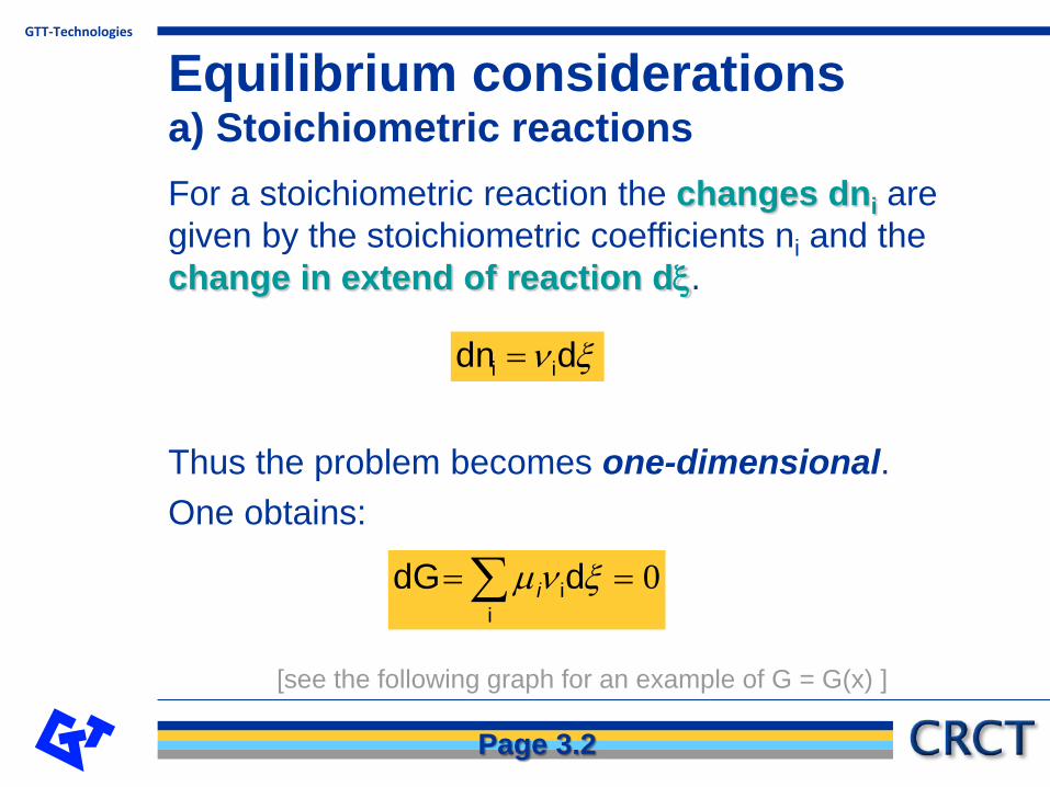
Equilibrium considerationsa) Stoichiometric reactions

Page 3.1

GTT-Technologies

For a stoichiometric reaction the changes dni are given by the stoichiometric coefficients ni and the change in extend of reaction dξ.

Thus the problem becomes one-dimensional.One obtains:

[see the following graph for an example of G = G(x) ]

ξν d dn ii =

0==∑i

id dG ξνµ i


Page 3.2

GTT-Technologies

Gibbs Energy as a function of extent of the reaction2NH3<=>N2 + 3H2 for various temperatures. It is assumed,that the changes of enthalpy and entropy are constant.

Extent of Reaction ξ

Gib

bs e

nerg

y G

0.0 0.1 0.2 0.3 0.4 0.5 0.6 0.7 0.8 0.9 1.0

T = 400K

T = 500K

T = 550K


Page 3.3

GTT-Technologies

Separation of variables results in :

Thus the equilibrium condition for a stoichiometric reaction is:

Introduction of standard potentials µi° and activities aiyields:

One obtains:

0== ∑i

ii µdξdG ν

0==∆ ∑i

ii µG ν

iii aRTµµ ln+=

( ) 0=+ ∑∑i

iii

ii aRTµ lnνν


Page 3.4

GTT-Technologies

It follows the Law of Mass Action:

where the product

or

is the well-known Equilibrium Constant.

∑ ∏−==∆i i

iiiiaRTµG νν ln

∏=i

iiaK ν


∆−=

RTGK

exp

The REACTION module permits a multitude of calculations which are based on the Law of Mass Action.

Page 3.5

GTT-Technologies

Electro-chemical equilibrium

e + ... + N + M = ... + B + A + e NMBA ββαα νννννν

The mass balance equation is now:

Including the effect of the electrons being on different electrical potential one obtains:

0=+∑ ∑ jjjii Fz ϕνµν

Page 4.1

GTT-Technologies

µνϕνϕνααββ iieeeeee = ) z - z - ∑( F

Separation of the electrons from the otherspecies leads to:

( ) ( ln )oe e e i i i i i iF RT aβ αν φ φ ν µ ν µ ν− = = +∑ ∑

Finally one obtains:

Two extreme cases can be distinguished.

ln i

oi i

ie e

RTE aF F

νν µν ν

= +∑ ∏Or: Nernst‘sequation

Page 4.2

GTT-Technologies

A simple concentration cell

The sketch of a lamnda-probe (for control of a car-catalyst).

Page 4.3

GTT-Technologies

βα | (air) O | ZrO | gas)(exhaust O 222 |

βα eairOOe 4)()gasexhaust (4 22 +=+

)gas exh.(

)air(

2

2

22ln)(4

O

OoO

oO p

pRTF +−=− µµϕϕ αβ

) pln - pln ( F 4T R

)gas exh.(O)air(O 22 = E

The Nernst-equation:

The cell scheme:

The cell reaction:

The simple end result:

Page 4.4

GTT-Technologies

The Hall-Heroult cell: Production of liquid aluminium from solid alumina

The decisive phase diagram:

Page 4.5

GTT-Technologies

The Hall-Heroult cell

βe 6 CO 1.5 O 3 C 1.5 2-2 +=+

Al2 Al2e 6 3 =+ +α

The cell sketch:βe 6 CO 1.5 O 3 C 1.5 2

-2 +=+

Al2 Al2e 6 3 =+ +α

Page 4.6

GTT-Technologies

The Hall-Heroult cell

βα CO2(G) Al, eelectrolytmolten C ,OAl 32

Al 2Al 2e 6 3 =+ +α βe 6 CO 1.5 O 3 C 1.5 2

-2 +=+

βα eGCOAlCOAle 6)(5.125.16 232 ++=++

a aa pln

6 +

6 5.1COAl

2Al

5.1CO

32

2

FRT

FG = E

o∆

The cell scheme:

The two half cells:

The total cell reaction:

The Nernst-equation (full and simple):

F 6G o∆ = E

Page 4.7

GTT-Technologies

Modelling of Gibbs energy of (solution) phases

Pure Substance (stoichiometric)

Solution phase

( ),pT,nGG immϕϕϕ =

),(,, pTGG oom

ϕϕϕ µ ==

( )ex

m

idm

idm

refmm

GSTG

GG

,

,

,

ϕ

ϕ

ϕϕ

+∆−=+

=

Equilibrium considerationsb) Multi-component multi-phase approach

Choose appropriate reference state and ideal term, then check for deviations from ideality.See Page 2.5 for the simple substitutional case.

Page 5.1

GTT-Technologies

Complex EquilibriaMany components, many phases (solution phases), constant T and p :

with

or

( )∑ ∑ +==i

ioi

iiii aRTnnG lnµµ

ϕ

ϕ

ϕm

m

im GnG

p

∑ ∑

=

min=G


Page 5.2

GTT-Technologies

Massbalance constraint

j = 1, ... , n of components b

Lagrangeian Multipliers Mj turn out to be the chemical potentials of the system components at equilibrium:

∑ =i

jiij bna

∑=j

jjMbG


Deviding the above equation by Σbj yields theequation of the well know common tangent !

Page 5.3

GTT-Technologies

System ComponentsPhase ComponentsFe N O C Ca Si Mg

Fe 1 0 0 0 0 0 0N2 0 2 0 0 0 0 0O2 0 0 2 0 0 0 0C 0 0 0 1 0 0 0CO 0 0 1 1 0 0 0CO2 0 0 2 1 0 0 0Ca 0 0 0 1 0 0 0CaO 0 0 1 0 1 0 0Si 0 0 0 0 0 1 0SiO 0 0 1 0 0 1 0

Gas

Mg 0 0 0 0 0 0 1SiO2 0 0 2 0 0 1 0Fe2O3 2 0 3 0 0 0 0CaO 0 0 1 0 1 0 0FeO 1 0 1 0 0 0 0

Slag

MgO 0 0 1 0 0 0 1Fe 1 0 0 0 0 0 0N 0 1 0 0 0 0 0O 0 0 1 0 0 0 0C 0 0 0 1 0 0 0Ca 0 0 0 0 1 0 0Si 0 0 0 0 0 1 0

Liq. Fe

Mg 0 0 0 0 0 0 1

Example of a stoichiometric matrix for the gas-metal-slag system Fe-N-O-C-Ca-Si-Mg

aij j

i


Page 5.4

GTT-Technologies

Use the EQUILIB module to execute a multitude of calculations based on the complex equilibrium approach outlined above, e.g. for combustion of carbon or gases, aqueous solutions, metal inclusions, gas-metal-slag cases, and many others .

NOTE: The use of constraints in such calculations (such as fixed heat balances, or the occurrence of a predefined phase) makes this module even more versatile.

Equilibrium considerationsMulti-component multi-phase approach

Page 5.5

GTT-Technologies

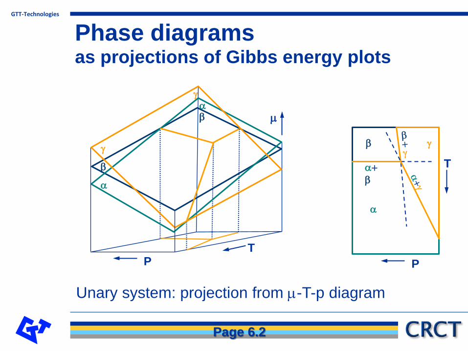
Phase diagrams as projections of Gibbs energy plotsHillert has pointed out, that what is called a phase diagram is derivable from a projection of a so-called property diagram. The Gibbs energy as the property is plotted along the z-axis as a function of two other variables x and y.

From the minimum condition for the equilibriumthe phase diagram can be derived as a projectiononto the x-y-plane.

(See the following graphs for illustrations of this principle.)

Page 6.1

GTT-Technologies

α

β γ

P

Tα+βα

β

γ

αβ

γ

µ

PT

Unary system: projection from µ-T-p diagram

Phase diagrams as projections of Gibbs energy plots

Page 6.2

GTT-Technologies

Binary system: projection from G-T-x diagram, p = const.

300

400

500

600

700

1.0

0.5

0.0

-0.5

-1.0

1.0 0.8 0.6 0.4 0.2 0.0

T

CuxNiNi

G


Page 6.3

GTT-Technologies

Ternary system: projection from G-x1-x2 diagram,T = const and p = const


Page 6.4

GTT-Technologies

Use the PHASE DIAGRAM module to generate a multitude of phase diagrams for unary, binary, ternary or even higher order systems.

NOTE: The PHASE DIAGRAM module permits the choice of T, P, m (as RT ln a), a (as ln a), mol (x) or weight (w) fraction as axis variables. Multi-component phase diagrams require the use of an appropriate number of constants, e.g. in a ternary isopleth diagram T vs x one molar ratio has to be kept constant.

Phase diagrams generated with FactSage

Page 6.5

GTT-Technologies

0i i i iSdT VdP n d q dµ φ+ + = =∑ ∑Gibbs-Duhem:

i i i idU TdS PdV dn dqµ φ= − + =∑ ∑

N-Component System (A-B-C-…-N)

SVnAnB⋅⋅⋅

nN

T-P µAµB⋅⋅⋅

µN

Extensive variables

Corresponding potentials

jqii q

U

∂∂

=φiq

Page 7.1

GTT-Technologies

N-component system(1) Choose n potentials: φ1, φ 2, … , φ n

(2) From the non-corresponding extensive variables(qn+1, qn+2, … ), form (N+1-n) independent ratios(Qn+1, Qn+2, …, QN+1).

Example:

Choice of Variables which always give a True Phase Diagram

( )1+≤ Nn

( )11 +≤≤+ Nin∑+

+=

= 2

1

N

nJj

ij

q

qQ

[φ 1, φ 2, … , φ n; Qn+1, Qn+2, …, QN+1] are then the (N+1) variables of which 2 are chosen as axes

and the remainder are held constant.

Page 7.2

GTT-Technologies

MgO-CaO Binary System

φ1 = T for y-axis

φ2 = -P constant

for x-axis

S T

V -P

nMgO µMgO

nCaO µCaO

Extensive variables and corresponding potentials

Chosen axes variables and constants

( )CaOMgO

CaO

CaO

MgO

nnnQ

nq

nq

+=

=

=

3

4

3

Page 7.3

GTT-Technologies

S T

V -P

nFe mFe

nCr mCr

f1 = T (constant)

f2 = -P (constant)

x-axis

x-axis

(constant)

Fe - Cr - S - O System

Fe

Cr

Fe

Cr

S

O

nnQ

nq

nq=

=

=

=

=

5

6

5

4

3

2

2

µφ

µφ

2

2

S

O

µ

µ

2

2

S

O

n

n

Page 7.4

GTT-Technologies

Fe - Cr - C System improper choice of axes variables

S T

V -P

nC µC

nFe µFe

nCr µCr

φ1 = T (constant)

φ2 = -P (constant)

φ3 = µC → aC for x-axisandQ4 for y-axis

(NOT OK)

(OK)

( )

( )4

4

Cr

Fe C

Cr

e

r

F Cr C

nQn n n

nQn n

=+ +

=+

Requirement: 0 3j

i

dQfor i

dq= ≤

Page 7.5

GTT-Technologies

This is NOT a true phase diagram.

Reason: nC must NOT be used in formula for mole fraction when aC is an axis variable.

NOTE: FactSage users are safe since they are not given this particular choice of axes variables.See next slide!

M23C6

M7C3

bcc

fcc

cementitelog(ac)

Mol

e fr

actio

n of

Cr

0

0.1

0.2

0.3

0.4

0.5

0.6

0.7

0.8

0.9

1.0

-3 -2 -1 0 1 2

Fe - Cr - C Systemimproper choice of axes variables

Page 7.6

GTT-Technologies

Fe - Cr - C Systemproper choice of axes variables

Calculation is donein Phase Diagrammodule withX = mole Cr/(Cr+Fe)and y = log a(C).

Axes are swapedin Figure module.

Page 7.7

GTT-Technologies

- Type 1 or Potential Diagrams:

Two potentials, Φi vs Φj.

- Type 2 or Mixed Diagrams:

One potential and one ratio ofconjugate extensive properties, Φi vs QΦ

j/ΣQΦk.

- Type 3 or Extensive Property Diagrams:

Two ratios of conjugate extensive properties, QΦ

i/ΣQΦk vs QΦ

j/ΣQΦk

Only three types of 2D-phase diagrams possible

Page 7.8

GTT-Technologies

Interrelationship of corresponding Type 1 (b), Type 2 (a,d), Type 3 (c) phasediagrams. (Φ4, Φ5 , ... are held constant; Φ3 is unspecified)

Pelton and Schmalzried, 1973

Page 7.9

the theoretical background of factsage - crct

Documents