the ’t hooft-loop in coulomb gauge - institut für...
TRANSCRIPT

The ’t Hooft Loop in Coulomb Gauge Eurograd Workshop Todtmoos 2007
Contents
� Coulomb Gauge Yang-Mills Theory
� The ’t Hooft Loop as confinement criterion
� Dependency of the ’t Hooft Loop behaviour on the Yang-Mills
vacuum
� Results for the ’t Hooft Loop
� Summary
arXiv:0706.0175 [hep-th]; Accepted for publication in Phys.Rev. D
Dominik Epple Page 1

The ’t Hooft Loop in Coulomb Gauge Eurograd Workshop Todtmoos 2007
Coulomb Gauge Yang-Mills Theory
� Hamiltonian formulation of Yang-Mills Theory
� Weyl gauge: A0 = 0, D.O.F are cartesian coordinates Aai (x),
canonically conjugated momenta Πai (x) = δ
iδAai (x),
ETCRs[Aa
i (x),Πbj(y)
]= iδabδijδ(x − y),
Hamiltonian H =∫
dxΠ2(x) + B2(x)
� Gauss’ Law DiΠi|Ψ〉 = ρm|Ψ〉 guarantees invariance of the
wave functional under small gauge transformations
� chose Coulomb Gauge ∂iAi(x) = 0 to resolve Gauss’ Law
Dominik Epple Page 2

The ’t Hooft Loop in Coulomb Gauge Eurograd Workshop Todtmoos 2007
Coulomb Gauge ∂iAi(x) = 0
� eliminates unphysical degrees of freedom,
� change of coordinates from cartesian to curvilinear ones,
� introduces Jacobian (Fadeev-Popov determinant)
J [A] = det(−∂iDi),
� new physical degrees of freedom are A⊥ai (x).
Dominik Epple Page 3

The ’t Hooft Loop in Coulomb Gauge Eurograd Workshop Todtmoos 2007
Coulomb Gauge Yang-Mills Hamiltonian
H =12
∫d3x
[J−1ΠaiJΠa
i + Bai Ba
i
]+
g
2
∫d3x
∫d3x′J−1ρa(x)F ab(x,x′)J ρb(x′)
Physically motivated ansatz for the vacuum wave functional
(strongly peaked at the Gribov Horizon J = 0)
Ψ[A] = J−12N exp(−1
2
∫d3xd3x′A⊥a
i ω(x,x′)A⊥ai (x′))
Dominik Epple Page 4

The ’t Hooft Loop in Coulomb Gauge Eurograd Workshop Todtmoos 2007
Find solutions for the Yang-Mills Schrodinger equation for the
lowest energy eigenstate form the variational principle
〈Ψ|H|Ψ〉〈Ψ|Ψ〉 → min .
� coupled set of integral equations (Dyson-Schwinger equations),
to be solved numerically1.
1C. Feuchter and H. Reinhardt, Phys. Rev. D70 (2004) 105021
Dominik Epple Page 5

The ’t Hooft Loop in Coulomb Gauge Eurograd Workshop Todtmoos 2007
Quantities which are computed self-consistently are
� Gluon form factor ω(q),〈ω|Aa
i (q)Abj(q
′)|ω〉 = 12(2π)3tij(q)δabδ(q − q′)ω−1(q)
� Ghost form factor d(q), Gω(q) = G0(q)d(q)/g,
G0(x,x′) = 〈x|(−∂2)−1|x′〉 = 14π|x−x′|
� Curvature χ(q), represents the ghost-loop part of the gluon
self-energy,
χ = −12〈δ2 lndet(−D∂)
δAδA 〉,J [A] = det(−D∂) = exp(− ∫
AχA)
Dominik Epple Page 6

The ’t Hooft Loop in Coulomb Gauge Eurograd Workshop Todtmoos 2007
The following IR behaviour holds to leading order:
ω(q) = χ(q) = A · k−α, d(q) = B · k−β, 2β − α = 1
The existence of two kinds of solutions has been predicted:
� One with α ≈ 0.795 (Found by C. Feuchter 2004)
� One with α = 1
We have been able to obtain also the solution with α = 1. Very
careful and elaborate numerics is required for it.
Dominik Epple Page 7

The ’t Hooft Loop in Coulomb Gauge Eurograd Workshop Todtmoos 2007
1
10
100
1000
0.001 0.01 0.1 1 10 100 1000
k [σ1/2]
ω(k) [σ1/2]χ(k) [σ1/2]
1
10
100
1000
10000
0.001 0.01 0.1 1 10 100 1000
k [σ1/2]
d(k)
Figure 1: (left) The Gluon dressing function ω(q) and the curvature χ(q), calculated by
minimizing the vacuum energy functional with a gaussian ansatz for the wave functional.
These curves are from the α = 1 solution. (right) Ghost dressing function d(q) from the
same calculation.
Phys.Rev.D75:045011,2007; hep-th/0612241
Dominik Epple Page 8

The ’t Hooft Loop in Coulomb Gauge Eurograd Workshop Todtmoos 2007
-5
0
5
10
15
20
25
0 2 4 6 8 10 12 14 16 18 20x/x0
[V(r)-V(1)]/k0Linear fit
Figure 2: The Coulomb Potential (quark-antiquark-Potential), computed with the form factors
from the solution with α = 1. We find a linear rising potential within excellent precision
(numerical error < 1%).
Dominik Epple Page 9

The ’t Hooft Loop in Coulomb Gauge Eurograd Workshop Todtmoos 2007
The ’t Hooft Loop as confinement criterion
The Wilson loop W [A(C)] = tr P exp(− ∮dxμAμ)
� Gauge-invariant quantity
� Measures magnetic flux through surface (for abelian theories)
Temporal Wilson Loop: Order parameter for Yang-Mills Theory
〈W [A(C)]〉 ={
exp(−σ · Area(C)), confined phase
exp(−κ · Perimeter(C)), deconfined phase
Dominik Epple Page 10

The ’t Hooft Loop in Coulomb Gauge Eurograd Workshop Todtmoos 2007
Spatial ’t Hooft loop V (C): defined via spatial Wilson Loop
V (C1)W (C2) = ZL(C1,C2)W (C2)V (C1)
with Z = −1 for SU(2) and L = Gaussian linking number.
’t Hooft loop behaviour:
〈V [A](C)〉 ={
exp(−κ · Perimeter(C)), confined phase
exp(−σ · Area(C)), deconfined phase
� dual to the Wilson loop’s behaviour.
(G. ’t Hooft, Nucl. Phys. B138 (1978) 1)
Dominik Epple Page 11
The ’t Hooft Loop in Coulomb Gauge Eurograd Workshop Todtmoos 2007
’t Hooft loop creates a Center Vortex (A(C) denotes a center
vortex field, W [A(C1)](C2) = ZL(C1,C2)):
V (C)Ψ[A] = Ψ(A + A)
Continuum Representation:
(H. Reinhardt, Phys. Lett. B577 (2003) 317-323)
V (C) = exp[i
∫d3xA(C)(x)Π(x)
]
Dominik Epple Page 12

The ’t Hooft Loop in Coulomb Gauge Eurograd Workshop Todtmoos 2007
The ’t Hooft Loop in Coulomb GaugeTo one-loop order, one can calculate
〈V (C)〉 =∫
DA det(−D∂)Ψ∗(A)Ψ(A + A)
= exp(−S(C)), S(C) := S(R)
S(R) = 4πR
∞∫0
dx K(x
R
)︸ ︷︷ ︸physics
π/2∫0
dα (1 − 2 sin2 α) f(2x sin α)
︸ ︷︷ ︸=:A(x), geometry
where f(z) = j0(z) − j′′0(z), j0(z) = sin z
z .
Dominik Epple Page 13
The ’t Hooft Loop in Coulomb Gauge Eurograd Workshop Todtmoos 2007
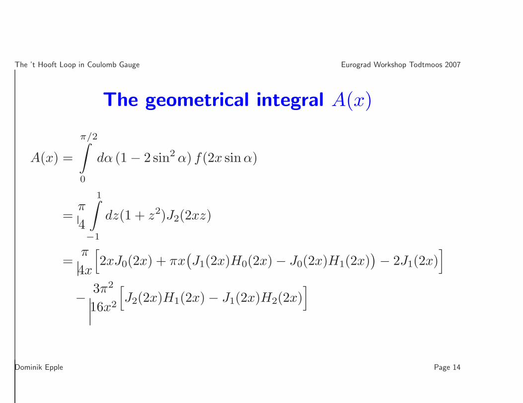
The geometrical integral A(x)
A(x) =
π/2∫0
dα (1 − 2 sin2 α) f(2x sinα)
=π
4
1∫−1
dz(1 + z2)J2(2xz)
=π
4x
[2xJ0(2x) + πx
(J1(2x)H0(2x) − J0(2x)H1(2x)
) − 2J1(2x)]
− 3π2
16x2
[J2(2x)H1(2x) − J1(2x)H2(2x)
]
Dominik Epple Page 14

The ’t Hooft Loop in Coulomb Gauge Eurograd Workshop Todtmoos 2007
The geometrical integral A(x)
0.001
0.01
0.1
1
0.1 1 10 100
A(x
)
x
Numerical value
Dominik Epple Page 15

The ’t Hooft Loop in Coulomb Gauge Eurograd Workshop Todtmoos 2007
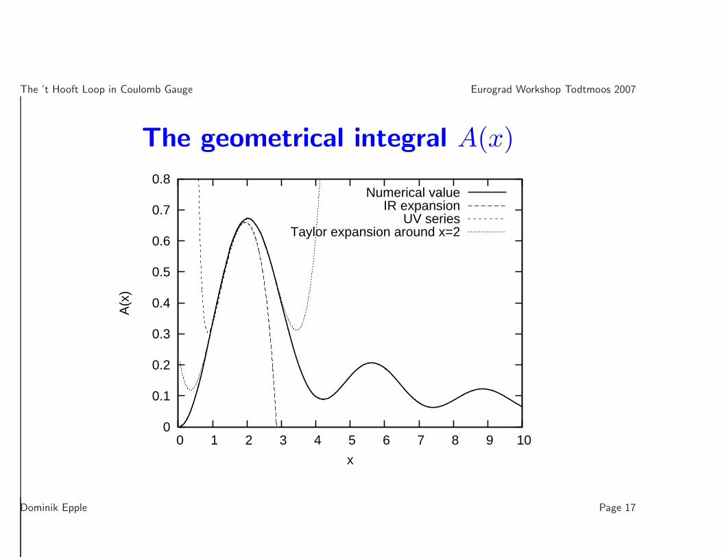
The geometrical integral A(x)Asymptotical properties:
� x → 0: A(x) = 2π15x2 − π
35x4 + O
(x6
)� x → ∞: A(x) = π
4x +√
π2 cos
(2x + π
4
)1√x3
+ O(
1√x5
)
0.001
0.01
0.1
1
0.1 1 10 100
A(x
)
x
Numerical valueIR expansion
UV seriesTaylor expansion around x=2
Dominik Epple Page 16
The ’t Hooft Loop in Coulomb Gauge Eurograd Workshop Todtmoos 2007
The geometrical integral A(x)
0
0.1
0.2
0.3
0.4
0.5
0.6
0.7
0.8
0 1 2 3 4 5 6 7 8 9 10
A(x
)
x
Numerical valueIR expansion
UV seriesTaylor expansion around x=2
Dominik Epple Page 17

The ’t Hooft Loop in Coulomb Gauge Eurograd Workshop Todtmoos 2007
Physics: K(q)
K(q) = [ω(q) − χ(q)][1 − 1
2[ω(q) − χ(q)]
ω(q)
]
=12ω(q)
[1 −
(χ(q)ω(q)
)2]
Asymptotic behavior:
� IR: K(q) IR= [ω(q) − χ(q)] ≈ c0 + c1 q + . . .
� UV: K(q) UV= 12ω(q) ≈ 1
2(q + a0) + . . .
Dominik Epple Page 18

The ’t Hooft Loop in Coulomb Gauge Eurograd Workshop Todtmoos 2007
Discussion of S(R)/R
S(R) = 4πR
∫dxK
(x
R
)A(x)
� Integral for S(R) linearly and logarithmically UV-divergent
� Large-R-behavior of S(R) tests IR-behavior of K(q)
� need to renormalize by subtraction of UV-leading parts in K(q)
Crucial: do not spoil IR-behavior!
Dominik Epple Page 19

The ’t Hooft Loop in Coulomb Gauge Eurograd Workshop Todtmoos 2007
Parametrize ω(q) = A/q + a0 + q.
Replace K(q) → K(q) − K0(q) = K(q):
K(q) =12ω(q)
[1 −
(χ(q)ω(q)
)2]
K0(q) =12(q + a0)
[1 −
(χ(q)ω(q)
)2]
K(q) =A
q
[1 −
(χ(q)ω(q)
)2]
Dominik Epple Page 20
The ’t Hooft Loop in Coulomb Gauge Eurograd Workshop Todtmoos 2007
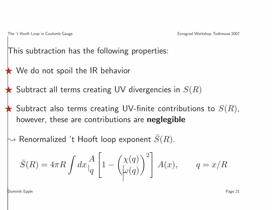
This subtraction has the following properties:
� We do not spoil the IR behavior
� Subtract all terms creating UV divergencies in S(R)
� Subtract also terms creating UV-finite contributions to S(R),however, these are contributions are neglegible
� Renormalized ’t Hooft loop exponent S(R).
S(R) = 4πR
∫dx
A
q
[1 −
(χ(q)ω(q)
)2]
A(x), q = x/R
Dominik Epple Page 21

The ’t Hooft Loop in Coulomb Gauge Eurograd Workshop Todtmoos 2007
Behaviour of the ’t Hooft Loop for differentsolutions of the YM vacuum
Using the asymptotic behavior of A(x), one can show that:
� A finite c0 leads to a logarithmically diverging S(R)/R
� c0 = 0 leads to S(R → ∞)/R → const., which corresponds to
a perimeter law for the ’t Hooft Loop.
These points can be verified numerically also with the full A(x).
Dominik Epple Page 22

The ’t Hooft Loop in Coulomb Gauge Eurograd Workshop Todtmoos 2007
Result for the ’t Hooft Loop
0
1
2
3
4
5
6
7
8
9
0 2 4 6 8 10 12 14 16 18 20
Sba
r(R
)/R
[G
eV]
R [fm]
ξ0=0, ξ= 0.15625ξ0=0, ξ= 0ξ0=0, ξ=-0.15625ξ0=1.44, ξ= 0.15625ξ0=1.44, ξ= 0ξ0=1.44, ξ=-0.15625
Figure 3: The S(R)/R function, calculated numerically using the full expression for A(x)
and the renormalized K(q) as described in the text. The YM-Solution has the property
ω(q) − χ(q) → 0 for q → 0. We see a behaviour of S(R → ∞)/R = const., which
means a perimeter law for the ’t Hooft loop, which corresponds to a confined theory.
Dominik Epple Page 23
The ’t Hooft Loop in Coulomb Gauge Eurograd Workshop Todtmoos 2007
Summary
� We have been able to obtain solutions for the Yang-Mills
vacuum which show a exact linear Coulomb potential.
� We can show a perimeter-law for the ’t Hooft Loop, i.e.
confinement, for a special solutions of the Yang-Mills vacuum.
Dominik Epple Page 24