the supreme court’s many median...

The Supreme Court’s Many Median Justices∗

Benjamin E. LauderdaleLecturer

Methodology InstituteLondon School of [email protected]

Tom S. ClarkAssociate Professor

Department of Political ScienceEmory University

[email protected]

February 7, 2012

ABSTRACT

Limitations in ideal point estimation methods have constrained the study of how pref-erences vary across areas of the law. Using multiple indices of substantive similarityamong cases, we apply a kernel-weighted optimal classification estimator to recover es-timates of judicial preferences that are localized to particular legal issues as well asperiods of time. Allowing preference variation across legal areas significantly improvesthe predictive power of estimated preference orderings versus a model that only allowsfor variation in preferences over time. We find there is substantial variation in the iden-tity of the median justice across areas of the law during all periods of the modern court,suggesting a need to reconsider empirical and theoretical research that hinges on theexistence of a unitary and well-identified median justice. The legal doctrines followedby Supreme Court justices are not reducible to simple left-right ideology.

∗We thank Chuck Cameron, Steve Haptonstahl, John Kastellec, Jeff Lax, Drew Linzer, Curt Signorino, and JeffStaton for helpful comments and discussions. This research was supported by an NSF Grant, Scaling Supreme CourtOpinions, Methodology, Measurement and Statistics (SES-0909235).

1. INTRODUCTION

Political scientists often argue that politics can be described succinctly and accurately as dominantly

unidimensional (Poole & Rosenthal 1997, Martin & Quinn 2002, Clinton, Jackman & Rivers 2004).

This claim has particular import in the context of judicial politics, where scholars have wrestled

with the question of whether, when, and how law and ideology interact. While the traditional

approach to judicial politics asserts that judges’ preferences are dominantly unidimensional and

independent of any legal considerations (e.g., Segal & Spaeth 2002), contemporary developments

in the literature argue that law and ideology must been seen as inextricably linked features of

judicial decision-making, rather than competing forces on judges (Lax 2011). Indeed, historical

accounts of the courts have documented instances of judges’ preferences varying across areas of the

law and over the course of their tenure on the bench (e.g., Greenhouse 2005, Jeffries 1994), and

recent developments in the literature have been particularly concerned with understanding how

Supreme Court justices systematically change their views across different areas of the law (e.g.,

Bailey & Maltzman 2008). Even so, empirical scholarship has been heavily channeled through the

unidimensional spatial model of justices’ preferences, at least in part because technical obstacles

make richer descriptions of preferences difficult to obtain systematically. As a result, we do not

know whether variation in preferences across areas of the law and over time is limited to a few

idiosyncratic examples, or whether it is instead a general feature of judicial preferences that should

shape the way we understand the Court’s internal decision-making and relationship to the broader

political system.

Claims by students of judicial decision-making that judges’ preferences are multidimensional

and intertwined with the law derive from qualitative contrasts of decisions in different areas of law

(e.g., Newman 1997, Stern & Wermiel 2010, Jeffries 1994). In this paper, we bring this insight to the

quantitative measurement of Supreme Court justices’ preferences, enabling systematic measurement

of how preferences vary across areas of the law and over time. To do so, we introduce a novel method

that recovers well-documented instances of variation in judicial preferences and also yields new

insights into the dynamics of decision-making in the U.S. Supreme Court. Our approach is based

1

on a further generalization of the optimal classification techniques introduced by Poole (2000) and

Bonica (2010) and is applicable to a number of small voting chambers other than courts, such as city

councils or the UN Security Council. The estimates that we present provide a richer view into the

justices’ preferences than do previous models that only allow preferences to vary across time (e.g.

Martin & Quinn 2002). We find a great deal of systematic variation in justices’ preferences beyond

simple left-right political ideology: the revealed judicial doctrines expressed through dispositional

votes vary substantially in their relative “liberalism/conservatism” across areas of the law. We find

evidence confirming well-documented instances of ideological shifts by justices over their careers,

but also that most justices remain stable in their relative preferences over time.

Perhaps most strikingly, we discover that the identity of the median justice—a figure whose im-

portance in institutional theories of judicial decision-making and separation-of-powers models can-

not be understated—is much more substantively and temporally varied than previously recognized.

This finding has implications for many substantive problems. Consider three examples. First,

theories of bargaining on the Supreme Court largely implicate the median justice (for an overview,

see Clark & Lauderdale 2010). Thus, while it is common to describe today’s Supreme Court as the

“Kennedy Court” because Justice Kennedy is seen as the median justice (Cole 2006, Alfano 2009),

our analysis reveals that during any given term the identity of the influential median justice varies

from case-to-case in ways that are predictable if one knows which issues are implicated by each

case. Indeed, during the October 2009 term, Kennedy found himself in the majority in only 5

of the 18 cases decided by a 5-4 margin, prompting leading Court observer Linda Greenhouse to

speculate that the Kennedy Court may be over and that the issues the Court is currently dealing

with may be dividing the justices along different cleavages (Greenhouse 2010). Second, studies of

Supreme Court nomination battles suggest a new nominee’s affect on the identity of the median

is an important factor in Senate approval (Moraski & Shipan 1999, Krehbiel 2007). Thus, when

assessing whether a new justice will affect the balance of the Court, one must consider variation in

the justices’ preferences across areas of the law to know when, where, and to what extent the new

justice’s vote may be pivotal. Finally, litigants who are seeking to advance their policy agendas

need to tailor their arguments to the critical members of the Court, which requires knowledge of

2

who is the median, or swing, justice (e.g., Baird 2007). Thus, if the cleavages that divide the Court

are in fact multidimensional, social scientific analyses of whether advocates can effectively target

the pivotal members of the Court will be led astray by an assumption that judicial politics are

unidimensional.

In the rest of this paper, we introduce an approach to evaluating substantive and temporal

variation in judicial preferences and then present novel insights about how preferences vary system-

atically. In Section 2, we describe how our approach to measuring Supreme Court preferences is

different from existing approaches. In Section 3, we describe our estimator in detail, as well as the

data that the estimator employs. Most importantly, we use two sources of information about the

substantive similarity of cases: expert coded categorical indicators of cases’ substantive “issues”

and “issue areas” from the Supreme Court Database (Spaeth, Epstein, Ruger, Whittington, Segal

& Martin N.d.) and distance in the citation network of majority opinions.1 Combined with the

timing of decisions, these data provide the information that our estimator requires to form prefer-

ence estimates situated at each case’s location within the law and in time. In Section 4, we validate

the preference variation recovered by the model by connecting our findings to existing qualitative

assessments of issue- and time-variation in justice preferences. In Section 5, we explore the impli-

cations our findings have for a variety of substantive problems at the core of research on judicial

institutions. Our analysis, we argue, opens the door to exploring several unexplored theoretical

and empirical problems. Section 6 offers concluding remarks.

2. AN ALTERNATIVE APPROACH TO CHARACTERIZING PREFERENCES

Estimation of political actors’ spatial preferences has a rich tradition in political science; in recent

years, the dominant approach has become likelihood or Bayesian estimates of cardinal preference

spaces. This approach rests on random-utility models that yield estimators similar or identical

to item-response theory models from psychometrics. The widely applied Martin-Quinn scores are

1While we deploy these auxiliary sources of information in a new way, our innovation is part of an ongoing trend

towards leveraging additional sources of information in the estimation of ideal points (e.g. Clinton & Meirowitz 2003,

Jessee 2009, Zucco, Jr. & Lauderdale 2011)

3

based on a dynamic model from this family. Multidimensional methods that describe positions

in two or more dimensions, based on varying underlying assumptions, have already been applied

to the U.S. Supreme Court (Grofman & Brazill 2002, Poole 2005, Peress 2009). While existing

multidimensional scaling methods have proved useful in understanding other roll-call voting data,

they are relatively ill-suited to the problem of characterizing variation in Supreme Court justices’

preferences across different kinds of cases. These methods face both identification and interpreta-

tion problems when applied to the U.S. Supreme Court—problems that motivate the alternative

approach that we follow.

2.1. Identifying Preference Dimensions on the Supreme Court

Recovering cardinal ideal point estimates, identifying additional dimensions beyond the first, and

making inter-temporal comparisons are all general problems in ideal point estimation. These prob-

lems are all exacerbated in the context of small voting bodies, such as the Supreme Court. Because

larger chambers have many more possible voting patterns than smaller chambers, larger chambers

provide much richer information about the structure of voting coalitions. Londregan (2000a) shows

that with a small number of voters, bill parameter estimates can only take on a small number of val-

ues because few voting coalitions are possible. This granularity of bill parameter estimates may lead

to inconsistency in ideal point estimates, regardless of how many votes are observed for each voter

and even if all other assumptions of the model are correct. This same lack of information about

bill (case) parameters has implications for scaling models’ ability to recover multiple dimensions.

Multidimensional scaling models attempt to infer how each case activates different preference di-

mensions from variation in the pattern of votes across different cases, precisely the information that

is lacking in small voting bodies because relatively few voting patterns are possible. Because there

are so few voters, the two-dimensional spatial preference maps calculated using differing methods

by Grofman & Brazill (2002), Poole (2005) and Peress (2009) are strikingly different in how they

arrange the Supreme Court justices.

Problems with inter-temporal comparability of estimates plague all ideal point estimators that

4

do not use substantive information about the content of roll-call votes to ensure that the same

locations on the scale have the same political content over time. Bailey (2007) anchors his estimates

of Supreme Court and congressional preferences using a collection of inter-temporal and inter-

chamber bridging observations, whereas Martin & Quinn (2002) rely on an assumption of local

stability in ideal points and a constant distribution of case parameters. The latter assumption is

a weak form of inter-temporal identification in a voting body like the Supreme Court, where large

fractions of the chamber can turn over in short periods of time and the population of cases may

be changing over time. Indeed, we have substantive reasons to worry about the inter-temporal

validity of the resulting estimates. For example, Martin-Quinn estimates of ideal points identify

the October 1972 term as the most conservative term between 1937 and 2009. That is, the median

justice’s ideal point is further to the right at that moment than at any other in the period. As

others have observed (Bailey 2007, 436), the October Term 1972 is the Supreme Court decided Roe

v. Wade by a vote of 7-2. Roe is just one case, but it is hard to reconcile the claim that the Roe

Court was the most conservative during that 73-year span, especially since Roe was only partially

upheld in Planned Parenthood v. Casey by a 5-4 vote in 1992. On the other hand, the first term

of the Roberts Court (the first part of the 2005 term) is identified in the Martin-Quinn scores as

having the left-most median justice since 1968. Few Court watchers would agree that the 2005

Court was comparable in liberalism to the Court of 1968; most would argue that the Court had

moved to the right during the 40 intervening years.

These and other instances stand as stark examples of the potentially misleading inferences that

may be drawn from IRT estimates of judicial ideal points that purport to be comparable cardinal

measures across all cases and time. Indeed, Ho & Quinn (2010) caution against relying on either

the cardinality or the inter-temporal comparability of Martin-Quinn scores. Thus, there is a strong

argument for generating descriptions of Court preferences that are limited to unidimensional rank

orderings of sets of justices who are on the Court simultaneously, the information that is most

strongly identified by dispositional voting data.2 Unfortunately, that stricture appears to rule

2Alternatively, one can make the additional assumptions necessary to use the bridging observations collected and

used by Bailey (2007).

5

out any characterization of how justices’ preferences vary across legal issues, at least with current

multidimensional scaling methods. However, those models are not the only way to summarize

the votes of Supreme Court justices. In the next part of this section, we describe an alternative

approach to characterizing how the preferences of justices vary across legal issues, one which has

advantages for the interpretation of issue-varying preferences as well as for the identification of such

variation.

2.2. Unidimensional Preferences in Case Subsets

The intuition for our approach follows most naturally if we begin with an example. Consider the

Supreme Court from October 1967 to May 1969. The Court handed down non-unanimous rulings

on 175 cases during these 19 months. We might reasonably ask whether justices express different

preferences through their dispositional votes in certain subsets of these cases. Roughly half (91) of

these 175 non-unanimous votes are in the “Criminal Procedure” and “Civil Rights” categories of

the Supreme Court Database. Using Poole’s (2000) optimal classification (OC) method in those

91 cases, we find the justices are ordered from left to right as follows: Douglas, Fortas, Brennan,

Marshall, Warren, Stewart, White, Harlan, Black. Applying the OC method to the remaining 84

cases, we find a justice ordering of Douglas, Fortas, Black, Warren, Brennan, Marshall, White,

Stewart, Harlan. These orders are very similar, with one major exception: Justice Black is the

right-most justice in the set of Criminal Procedure and Civil Rights cases but is third from the left

in all the other cases.3 This is a substantively large difference in location.4 Put directly in terms of

voting, the most common coalitions of justices in these two issue areas during this period of time

are different from the most common coalitions of justices in other issues areas.

In the preceding example, we have taken a set of cases, and instead of finding a single uni-

dimensional preference ordering of justices or a multidimensional preference map of justices, we

have estimated two unidimensional orderings that each apply to disjoint subsets of the cases, with

3The justice orderings under an IRT model exhibit a similar difference in the location of Justice Black.4In this instance it may be partly due to the small number of cases considered, but in general this kind of

comparison is a natural one to make.

6

the subsets defined by an auxiliary source of data about which cases share certain similarities (an

expert coding of the subject of individual cases). Our approach, which we describe fully in Section

3, simply takes this logic much further. We allow for different orderings in every case.5 For each

case, the estimated ordering depends primarily on voting behavior in the set of other cases that are

most substantively and chronologically proximate, given our auxiliary sources of data. Estimation

details aside, this is a conceptually different way to describe preferences from that of standard mul-

tidimensional ideal point estimation. But why does it makes sense to take this novel approach to

describing the preferences of justices? Why not estimate justice locations in a higher dimensional

space using an existing estimator?

While one advantage of our approach over this alternative is relative ease of identification,

perhaps more important is the relative ease of interpretation. On the basis of the example above,

we were able to make the statement that Justice Black was more conservative relative to other

justices in Criminal Procedure and Civil Rights cases than he was in other cases during the natural

court running from October 1967 to May 1969. Statements of this kind—justice X is relatively

liberal/conservative in some area of the law—are not easy to make from the perspective of standard

multidimensional ideal point estimators. Instead, in standard multidimensional models this kind

of statement would be made indirectly from an analysis of the relative positions of justices in the

different dimensions combined with a considering of how a given vote divided justices in those

dimensions.

Statements about variation in justices’ relative liberalism/conservatism and the identity of the

Court median directly implicate the most widely applied theories of the Court. In the example

above, we can see that Chief Justice Warren is estimated to be the median in Criminal Procedure

and Civil Rights; Justice Brennan is estimated to be the median in the remaining areas. This kind

of statement is potentially important for evaluations of the many theories of the Court which imply

a distinctive role for the median justice. Indeed, Martin, Quinn & Epstein (2005, 1280) observe

that the “[i]n the contemporary study of judicial politics, it is difficult to identify research that

5To be clear, as in this example, we assume a unidimensional ordering, but simply allow a different ordering (or,

dimension) for each case.

7

does not represent the Court on the basis of the preferences of the ‘median Justice’ or otherwise

make use of that concept.” Yet, from the perspective of standard multidimensional ideal point

estimators, it is very hard, if not impossible, to talk about median justices. There is no median

voter for multidimensional spatial preference maps.6

Our quantities of interest, then, are the relative propensities of each justice to vote for each of

the two sides of a case in a given area of law decided at a given time. For a single case, this is a

unidimensional quantity, but one for which the justices’s relative ordering may not be the same for

all cases. The estimation problem is one of in-sample prediction: given all of the Supreme Court

decisions other than case t, what is our best guess about the relative propensity of the justices to

vote for either side in case t? To answer this question, it might turn out that justices’ decisions

in all other cases are equally informative about justices’ decisions in case t. Intuitively, though,

it seems more likely that some cases are more informative than others, and so they ought to have

higher predictive weight for case t. In particular, we expect that cases involving similar issues or

decided at about the same time would be the best indicators of the likely preferences of the justices

in case t. If we have data about which cases are most likely to be relevant to predicting preferences

in case t, we can can put higher weight on those cases, and assess whether in-sample prediction

is improved. This is a data-driven form of “multidimensionality”. If our auxiliary data about

case similarity does not predict variation in justices’ preferences, then we will recover the same

unidimensional preference ordering for all cases because the same set of cases with the same set of

weights are used to predict voting in all cases. We also preserve interpretability: our estimates of

the preference ordering for case t are our best guess at the relative propensity of each justice to

vote in a given direction in that case, based on the most substantively and chronologically similar

cases.

Estimating case-specific preferences for justices might appear to violate the spirit of ideal point

estimation as a data reduction exercise. Indeed, compared to a single unidimensional ordering, our

approach yields a less parsimonious description of decision-making. However, our estimates are

built on much more extensive information than conventional ideal point estimates: we combine the

6Except in the degenerate cases described by Plott (1967).

8

roll-call (vote) matrix with multiple sources of auxiliary data about which votes are substantively

and temporally similar. Because we use richer data, the summaries of justices’ decisions that result

from our approach can convey a more nuanced and accurate account of judicial decision-making.

3. DATA AND METHODS

3.1. Data

We begin with the same matrix of justices’ dispositional votes on cases that form the basis for

previous studies of Supreme Court preferences (Martin & Quinn 2002, Grofman & Brazill 2002,

Bailey 2007, Peress 2009). These data are drawn from the Supreme Court Database (Spaeth

et al. N.d.). There are 4186 non-unanimous majority decisions between 1953 and 2006 for which

we have all necessary data sources, which cover at least part of the careers of 29 justices. The

dispositional vote for justice i in case t is coded Yi,t ∈ {0, 1}, where 1 corresponds to a majority vote.

We exclude unanimous cases because they convey no information about the preference orderings

of justices.7 Overall, in these data, there are 25,428 majority votes and 10,728 dissenting votes.

For our approach, we need an additional kind of data: measures of the similarity among cases.

We have three kinds of similarity measures between any pair of Supreme Court decisions: one

chronological and two substantive. The first measure is the number of years between two decisions

Tt,t′ , which is drawn from the Supreme Court Database (Spaeth et al. N.d.). We use years, rather

than a smaller unit of time or the ordinal ordering of decisions, because we do not expect justices to

change their doctrinal perspectives on time-scales shorter than a year.8 Various factors, including

the nature of the decisions themselves, can influence precisely when cases are officially decided

7These cases can be included at no cost other than computation time.8An anonymous reviewer noted that there is an argument for also using a measure of distance in terms of natural

courts to reflect the possibility that court composition changes the cert process or otherwise leads to substantively

important shifts in the justices’ decision-making. As will become clearer below, our approach does place less weight

on votes in different natural courts from that of case t because the number of possible misclassifications in a case t′

declines with the number of justices shared with the case t Court for which we are estimating an ordering.

9

within a term, which could induce biases if we tried to use a more finely-grained measure of

temporal similarity.

The second (dis)similarity measure is a three-level distance measure derived from expert codings

of the substantive issue at hand in each case. The Supreme Court Database assigns to each case

an “issue” and “issue area” code, which identify the primary substantive legal questions at stake

in each case. The broader “issue area” is a 13-category classification; within each of these areas

there are varying numbers of narrower “issues”. We convert these issue area and issue codes into a

trichotomous measure of distance, It,t′ . If two cases are in the same issue It,t′ = 0; if they are in the

same issue area but not the same issue, It,t′ = 1; and if they are in different issue areas, It,t′ = 2.

We explored separating this into two binary distance measures, but found that there was negligible

gain from the more flexible model.9

The third (dis)similarity measure makes use of data on citations between majority opinions,

which is based on Shephard’s citations (a database maintained by LEXIS which identifies all ci-

tations among Supreme Court opinions). Where each case is a network node, each citation forms

a direct link between two of those nodes. By calculating the minimum number of these links re-

quired to travel between case t and case t′, we generate a citation network distance measure Ct,t′ .10

For example, to reach the search and seizure case Mapp v. Ohio (1961) from the abortion rights

case Roe v. Wade (1972), the shortest distance is 2 citations. One such path is via the search and

seizure case Katz v. United States (1967). Katz cites Mapp as an important precedent in search and

seizure jurisprudence. Roe then cites Katz as one of several cases in which the Court recognized a

constitutional right to personal privacy not explicitly indicated in the text of the Constitution. We

consider chains of citation going both forward and backward in time: Katz was decided after Mapp

and before Roe, but is considered to be one unit of distance from both cases. These three cases

are all, to varying degrees, related to the issue of privacy, and so it is not surprising that they are

relatively close together in the citation network. Most Supreme Court cases are connected within

six degrees of citation, none is further than eight, and nearly the entire network is connected.11

9For reasons that will become clear below, the computational complexity of cross-validation increases significantlyif this distance measure is split in two.

10We include unanimous decisions when calculating citation network distance.11The disconnected opinions are short opinions with no citations to any other decision in the data. These discon-

10

3.2. Kernel-Weighted Optimal Classification

To combine these sources of information about preferences (justices’ votes) and about case similarity

(year, Spaeth issue, and citation network distance), we use a variant on optimal classification

techniques. In one dimension, optimal classification is based on a spatial voting model in which the

justices are arranged in rank order from left to right, and each vote is characterized by a cutting line

that separates voters who are predicted to vote way from voters who are predicted to vote the other

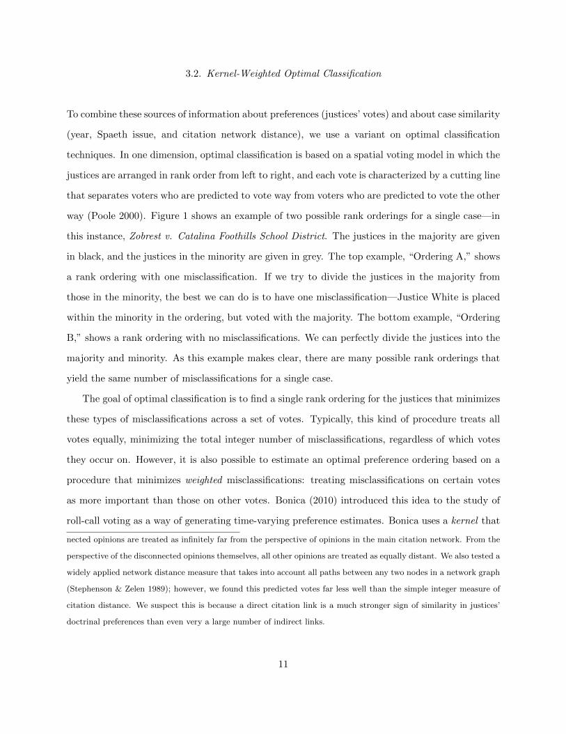
way (Poole 2000). Figure 1 shows an example of two possible rank orderings for a single case—in

this instance, Zobrest v. Catalina Foothills School District. The justices in the majority are given

in black, and the justices in the minority are given in grey. The top example, “Ordering A,” shows

a rank ordering with one misclassification. If we try to divide the justices in the majority from

those in the minority, the best we can do is to have one misclassification—Justice White is placed

within the minority in the ordering, but voted with the majority. The bottom example, “Ordering

B,” shows a rank ordering with no misclassifications. We can perfectly divide the justices into the

majority and minority. As this example makes clear, there are many possible rank orderings that

yield the same number of misclassifications for a single case.

The goal of optimal classification is to find a single rank ordering for the justices that minimizes

these types of misclassifications across a set of votes. Typically, this kind of procedure treats all

votes equally, minimizing the total integer number of misclassifications, regardless of which votes

they occur on. However, it is also possible to estimate an optimal preference ordering based on a

procedure that minimizes weighted misclassifications: treating misclassifications on certain votes

as more important than those on other votes. Bonica (2010) introduced this idea to the study of

roll-call voting as a way of generating time-varying preference estimates. Bonica uses a kernel that

nected opinions are treated as infinitely far from the perspective of opinions in the main citation network. From the

perspective of the disconnected opinions themselves, all other opinions are treated as equally distant. We also tested a

widely applied network distance measure that takes into account all paths between any two nodes in a network graph

(Stephenson & Zelen 1989); however, we found this predicted votes far less well than the simple integer measure of

citation distance. We suspect this is because a direct citation link is a much stronger sign of similarity in justices’

doctrinal preferences than even very a large number of indirect links.

11

StevensBlackmun

WhiteSouter

O'ConnorKennedy

Rehnquist

ThomasScalia

1 2 3 4 5 6 7 8 9

StevensBlackmun

SouterO'Connor

KennedyWhite

RehnquistScalia

Thomas

Ordering B

Ordering A

Figure 1: Example rank orderings using optimal classification, Zobrest v. Catalina Foothills SchoolDistrict (1993). Figure shows two possible rank orderings for the nine justices deciding Zobrestv. Catalina Foothills School District. Ordering A shows an ordering with one misclassification;Ordering B shows an ordering with no misclassifications. Names in grey are justices in the caseminority; names in black are justices in the case majority.

puts more weight on avoiding misclassifications in more chronologically proximate votes, yielding an

estimator that recovers different unidimensional orderings for different moments in time as the set

of cases receiving the most weight changes. We extend this approach to the problem of estimating

preferences that vary across both time and issues. Our approach is to use a kernel that weights votes

in other cases not just by their chronological proximity but also by their substantive similarity. In

addition to assessing temporal variation in judicial preferences by using a kernel weighting function

that discounts misclassifications in chronologically distant cases, we assess variation in judicial

preferences across legal issues by using a kernel that also discounts voting behavior in cases that

are distant in our two issue measures. This enables us to generate estimates of the preference

ordering that are particular, or localized, to each case in our data set. Thus, in describing the

estimation procedure, we will frequently refer to estimates for “the case under consideration” to

reference the particular case for which we are estimating a rank ordering.

12

Kernel Weighting. To weight misclassifications, we use the following exponential product kernel

function:

wtt′ =

0 if t = t′

αIt,t′ · βCt,t′ · τTt,t′ if t 6= t′(1)

When estimating the ordering in case t, the votes in case t itself receive no weight (wtt = 0). We

omit the votes in the case under consideration from the estimation of the preference ordering in

that case to avoid over-fitting and to facilitate meaningful assessment of whether our approach

improves predictive power versus a constant unidimensional ordering.12

When estimating the ordering in case t, the votes in every other case, t′, receive a weight, wtt′ ,

corresponding to their substantive and temporal similarity. The relative degree to which the kernel

discounts votes in the three dimensions of similarity is determined by three bandwidth parameters.

These parameters, α ∈ (0, 1], β ∈ (0, 1] and τ ∈ (0, 1], determine the weight given to each of

the three measure of similarity: issue area, citation distance, and time, respectively. For all three

of these parameters, smaller values correspond to more local estimates in which justice orderings

vary over small distances in the similarity measures, while higher values correspond to more global

estimates in which justice orderings vary only across larger distances in the similarity measures.

To generate an intuition for this kernel function, is is instructive to consider the special cases

for each of the three parameters. If α = 1, Spaeth issue does not affect the weight assigned to

cases. As α gets closer to 0, cases from different Spaeth issues and issue areas are increasingly

discounted when estimating the rank ordering in the case under consideration. If β = 1, distance

in the citation network does not affect a case’s weight. As β gets closer to 0, more weight is put on

the cases that cite or are cited by the case under consideration. If τ = 1, case weights are invariant

to chronological distance. As τ gets closer to 0, more weight is put on cases that were decided in

the same year as the case under consideration. Thus, when α = β = τ = 1, all cases are weighted

12For purely descriptive applications, one might include each case in the estimates at that case. If one does this, one

should do it lexicographically, considering only the preference orderings that are compatible with the dispositional

votes in that case. The major difficulty of this approach is that it becomes difficult to specify left and right without

auxiliary data about case polarity; but, combined with information in the Supreme Court database, this could be a

useful approach for some applications.

13

equally, and we recover constant unidimensional orderings (the preference ordering is the same in

each case). In our discussion below, we often use the constant ordering model as a baseline and

refer to it as the constant ideal point model.13

Estimation Strategy. Though the objective function for kernel-weighted optimal classification

is simple—the number of misclassifications for a given justice ordering multiplied by their case-

specific kernel weights, summed across cases—we must specify a procedure for finding the justice

orderings that optimize this objective function. One candidate approach is Poole’s Eliza algorithm,

which alternates between finding the best cut-points and the best voter-ordering. Unfortunately,

this algorithm can get “stuck” at suboptimal orderings when there are very few voters, which makes

it an unreliable estimation strategy for voting bodies as small as the U.S. Supreme Court (see Poole

2000, Tahk 2006). Bonica’s (2010) estimator for weighted optimal classification is based on this same

optimization procedure, so it inherits the same problem if applied to small legislatures. Fortunately,

the small size of the Court enables alternative approaches to optimization. Our estimation strategy

is a nested optimization process, described in the following two paragraphs. The first of these

describes how we find the best orderings for each case in our data, given particular values for

the bandwidth parameters. The second of these describes how we find the best set of bandwidth

13While the functional form of the kernel is usually far less important in non-parametric estimation than is finding

appropriate values for bandwidth parameters (Wasserman 2005, 72), the exponential functional form is particularly

attractive for this application. First, for Spaeth categories, the functional form is very simple: a multiplicative

penalty for being in a different issue and the same penalty again for being in a different issue area. Second, for

network distance, an exponential decay is a natural choice because the number of cases at a given network distance

grows approximately exponentially for short distances. Therefore, to have a truly local estimate the kernel must

penalize distance (at least) exponentially. Third, for time, we use the same exponentially decaying kernel as for

the issue distances because it ensures that the estimation procedure can make tradeoffs between the importance

of chronological and issue proximity. Our choice to use a kernel with infinite support rather than one with finite

support reflects the fact that we have multiple distance measures. The tricubic kernel used by Bonica (2010) has

finite support, which is appropriate given that he only weights by a single chronological distance measure and there

are always sufficient votes within the moving window defined by his kernel. However, to make tradeoffs between case

pairs that are close in time and far in issue and case pairs that are far in time and close in issue, it is necessary to

have a kernel function that is never exactly zero, as can be the case for kernels with finite support.

14

parameters in order to minimize misclassifications.

For given values of each of the three bandwidth parameters, we find the optimal rank orderings

for each case as follows. We start with the first case in the data and rank the justices participating

in the case randomly. We then identify all other cases in which at least three justices from the

target case participated.14 We then calculate the total number of weighted misclassifications that

result from each of the 18 possible cutpoint locations and polarities of the ordering in each of the

other cases with at least three justices in common,15 with the weighting determined by the kernel

function. Then we try every other possible ordering that can be reached by moving one justice to a

new location in the ordering, and assess whether the weighted classification score improves.16 We

adopt the justice ordering that yields the least weighted misclassifications, and repeat this search

for single justice moves that improve weighted classification until there are none remaining.17 This

yields our estimated ordering for the first case in the data set, and yields a count of misclassifications

when applied to that case. We repeat this search procedure for every case in the data and sum the

resulting integer misclassifications that result from applying the resulting case-specific estimated

orderings to each of those cases. This procedure yields an integer number of total misclassifications

across the entire data set, conditional on the bandwidth parameters: E(α, β, τ).

Because this number of misclassifications is conditional on the bandwidth parameters, we must

specify a procedure for identifying the best parameter values. Since we have omitted the votes

in the target case from the estimation of preferences for that case, we can use E(α, β, τ) as a

leave-one-out cross-validation score for the in-sample predictive power of the model. In general,

14No misclassifications can occur with less than three voters.15The justices could be divided at any point, and the majority could be on the left or the right.16Each of the 9 justices can be moved to 8 alternative locations while keeping the other justices in the same order;

however, each of the 8 possible swaps of adjacent justices can be generated by moving either of the two justices, so

there are 9 × 8 − 8 = 64 possible alternative rank orderings. We thank a reviewer for noting that we were failing to

take advantage of these redundant moves.17As a final step, we fix the polarity for each ordering of justices such that Justice Douglas is on the left and

Justice Rehnquist is on the right. We choose these justices because they span the entire period under study with

the minimum number of constraints, and their alignments were among the most consistent of all justices. Even so,

because our orderings are case-specific, occasionally one of these justices is estimated to be the median. In such cases,

the polarity of the Court is indeterminate. This is a problem for very few cases.

15

cross-validation methods are based on the idea of training (fitting) a model using a subset of the

data and then testing the resulting estimates by predicting the remaining observations. Leave-

one-out cross-validation is the special case of cross-validation where the withheld test data set is

a single observation: the model is fit once for each observation, each time leaving that particular

observation out of the data. The cross-validation score—the quantity to be minimized—is then the

sum or average of the errors in predicting every observation in the data, when those observations

were omitted from the estimation.

The optimal values of the bandwidth parameters involve balancing a tradeoff between our desire

to use only relevant cases in estimating preferences and our need to use a sufficient number of cases

in order to make reliable estimates. If the bandwidth parameters are too small, prediction will

suffer because very few cases will have any weight in the estimation of the ordering for a given case,

and our estimates will be noisy as a result. If the bandwidth parameters are too large, prediction

will suffer because too much weight is put on cases that are chronologically or substantively distant

and our estimates will not vary enough across issue and time. The best bandwidth parameters will

be those that give the optimal level of partial pooling—the model will rely heavily on decisions in

the most similar cases when there are many similar cases but rely instead on the larger pool of less

similar cases when the given case has few similar cases (in terms of time and issue). However, even

though cross-validation imposes no additional cost over fitting the model once, because we omit

case t anyway, we do have to re-estimate the entire model for every set of bandwidth parameters

we wish to consider. As a consequence, computation time is a constraint on the procedures that we

can use for optimization of the bandwidth parameters.18 To keep computation time tractable, we

used a hybrid procedure, beginning with a hill-climbing procedure to find approximately optimal

bandwidth values. Since the number of misclassifications is an integer, this procedure eventually

gets stuck, at which point we switched to a local three dimensional grid search on a spacing of 0.01.

We report statistics on how the fit of the model depends on the bandwidth parameters in Section

4.

18With compiled C++ code (using the Rcpp and inline packages for R (Eddelbuettel & Francois 2011, R Devel-

opment Core Team 2008)) and a 2011 vintage computer, estimating orderings for all cases in our data with a single

set of bandwidth parameters takes about 10 minutes.

16

3.3. Features and Limitations

There are three features of our model that bear brief discussion. The first concerns our assumption

that orderings within cases are unidimensional. While Supreme Court cases present complex ques-

tions, the decision at hand in any given case ultimately boils down whether to affirm or reverse the

lower court. While we do occasionally observe different vote coalitions across different questions

raised in a case, the fact that the Court requires cases to be narrowly focused and concerned with a

limited number of legal questions suggests that a unidimensional model within each case is a useful

approach to modeling judicial votes. Of course, further refinements to our model are possible, in

which distinct votes within a case are coded separately (Spaeth et al. N.d.) and opinion texts are

divided into distinct sections from which the relevant citation network distances are calculated.

A second, related, feature of our model is that our estimation procedure guards against over-

fitting by excluding the votes in a given case from the estimation of the justice ordering for that

case. This is important because it provides a principled way to determine how much preference

variation is present across time and issue. However, we have not found a way to generate satisfac-

tory measures of uncertainty for our estimator. The interrelated nature of judicial decision-making

is a severe obstacle—both conceptually and practically—to using resampling methods to generate

bootstrap uncertainty estimates. The observed cases are the exhaustive set of all Supreme Court

decisions and they are fundamentally interdependent, not only through the ways that justices’

dispositional votes sometimes depend on previous court decisions, but also through the citation

process. Citation distances would change under re-sampling, making it difficult to define an appro-

priate procedure that captures our substantive uncertainty about judicial preferences. Thus, while

one might calculate bootstrap uncertainty estimates for our model, we have chosen not to in order

to guard against misinterpretation of those quantities.

The third feature that bears discussion concerns the utility of our model for making out-of-

sample predictions. Our model can easily be applied to do so, requiring only the generation of

suitable proxies for the missing measures of substantive distance. With respect to the issue measure,

the coding rules for this variable are publicly available and can easily be applied to any potential

17

case coming before the Court. With respect to the measure of citation distances, one could generate

this measure by looking to the citation patterns in the appellate court majority opinion or briefs

filed by the litigants, the sources on which much of the language and cited doctrine in Supreme

Court opinions draw (Spriggs & Hansford 2002). Predicted rank orderings for such a hypothetical

case could then be generated by using the resulting kernel weights given the estimated bandwidth

parameters and the proxied data on substantive similarity. While we do not explore this out-of-

sample prediction problem in this paper, it has potential applications to studies of the Court’s

decisions to grant certiorari (the choice whether to hear a case), as well as to predicting likely

justice alignments in cases on the Court’s docket.

4. RESULTS AND VALIDATION

We now review the primary results from our estimation. Our discussion serves two purposes. First,

we demonstrate systematic variation in justices preferences over time and across substantive areas

of the law. In doing so, we are able to compare the relative predictive power of each of the sources

of similarity that we have included in our estimator. We are also able to describe the extent to

which different areas of the law are associated with more varied preferences and which areas of the

law are associated with common preference orderings among justices. Second, through our analysis

of these results, we document several well-known (and other less well-known) instances of variation

in particular justices’ preferences. This evidence helps serve to establish the validity of our model.

4.1. Relative Predictive Power of Issue, Citation and Chronological Distances

We begin our analysis by comparing the relative predictive power of the three sources of dissimilarity

we included in our model. To do so, we identify the number of misclassifications under a variety

of possible combinations of bandwidths for each of the various parameters. In the first column

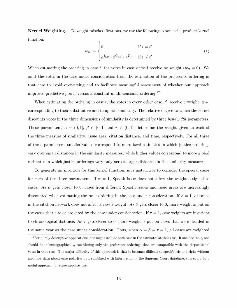
of Figure 2, we report the results of cross-validation and the misclassification rates of the best

models we find as a function of time and issue areas. As a baseline, we consider first the case where

18

0.0

0.2

0.4

0.6

0.8

1.0

2600280030003200340036003800

Ban

dwid

th

Misclassifications

Alp

haB

eta

Tau

Alp

ha (

Ran

dom

ized

)B

eta

(Ran

dom

ized

)Ta

u (R

ando

miz

ed)

Bandw

idth

Mis

class

ifica

tions

Model

αβ

τC

ount

Red

uct

ion

vs.

Unanim

ity

vs.

Const

ant

Unanim

ity

--

-10728

0.0

00

-C

onst

ant

11

13148

0.7

07

0.0

00

Tim

e-O

nly

11

0.1

82944

0.7

24

0.0

65

Cit

ati

on-O

nly

10.0

71

2833

0.7

36

0.1

00

Issu

e-O

nly

0.0

61

12792

0.7

40

0.1

13

All

0.3

00.1

80.7

52534

0.7

64

0.1

95

1960

1970

1980

1990

2000

0.00.20.40.60.81.0

Year

Average Misclassifications per Case

Con

stan

tS

paet

hC

itatio

nT

ime

Bes

t

Ave

rage

Mis

clas

sific

atio

ns p

er C

ase

Spaeth Issue Area

0.0

0.2

0.4

0.6

0.8

1.0

1.2

n=10

94

n=73

7

n=42

4

n=15

8

n=56

n=46

n=17

2

n=71

2

n=39

9

n=16

4

n=17

n=14

6

n=13

Crim

inal

Pro

cedu

re

Civ

il R

ight

s

Firs

t Am

endm

ent

Due

Pro

cess

Priv

acy

Atto

rney

s

Uni

ons

Eco

nom

ic A

ctiv

ity

Judi

cial

Pow

er

Fed

eral

ism

Inte

rsta

te R

elat

ions

Fed

eral

Tax

atio

n

Mis

cella

neou

s

Con

stan

tS

paet

hC

itatio

nT

ime

Bes

t

Fig

ure

2:R

esu

lts

from

cross

-vali

dati

on

an

dm

odel

com

pari

son

.T

he

left

colu

mn

show

sth

ere

sult

sof

cros

s-va

lid

atio

n.

Th

eto

ple

ftfigu

resh

ows

the

tota

lnu

mb

erof

mis

clas

sifi

cati

ons

wh

enop

tim

izin

gea

chb

and

wid

thp

aram

eter

ind

ivid

ual

ly,

wh

ile

hol

din

gth

eot

her

two

at

1,

usi

ng

the

tru

eca

sed

ata

and

ran

dom

lyre

sam

ple

dca

sed

ata.

Th

eb

otto

mle

ftta

ble

show

sth

eop

tim

alva

lues

ofth

eb

an

dw

idth

par

amet

ers

and

the

corr

esp

ond

ing

rate

sof

mis

clas

sifi

cati

onfo

rm

od

els

that

allo

wn

one,

one,

oral

lof

the

ban

dw

idth

para

met

ers

tova

ryfr

om

1.(W

hen

ab

and

wid

thp

aram

eter

iseq

ual

to1,

the

sou

rce

ofsi

mil

arit

yd

oes

not

affec

tth

era

nk

ord

erin

gs.

Th

ecl

oser

the

ban

dw

idth

para

met

eris

toze

ro,

the

less

wei

ght

dis

sim

ilar

case

sh

ave

onth

ees

tim

ated

ran

kor

der

ings

.)T

he

right

colu

mn

com

pare

sm

iscl

ass

ifica

tion

rate

sfo

rth

eb

otto

mfi

vem

od

els

from

the

low

erle

ftta

ble

asa

fun

ctio

nof

sub

stan

tive

vari

able

s.T

he

top

righ

tfi

gu

resh

ows

the

rate

ofm

iscl

assi

fica

tion

sp

erdec

isio

nov

erti

me.

Th

elo

wer

righ

tfi

gure

show

sth

era

teof

mis

class

ifica

tion

sp

erdec

isio

nfo

rea

chof

the

13S

pae

this

sue

area

s.

19

α = β = τ = 1, a constant ideal point model in which justices’ preferences do not vary across time

or area of the law (the rightmost point in the top left panel of Figure 2). This model results in a

total of 3148 misclassifications across the set of cases we consider, compared with a naive baseline

model assuming all cases are unanimous, which results in 10,728 misclassifications.

We then identify the optimal bandwidth for each of the other parameters—Spaeth issue code,

citation network distance, and year of decision—holding the other two parameters at 1 (the minima

in the top left panel of Figure 2). We find that using the Spaeth issue and issue area codes leads

the the greatest reduction in misclassifications (11.3%, from 3148 to 2792), followed by citation

network distance (10%, from 3148 to 2833), followed by chronological distance (6.5%, from 3148 to

2944). In other words, preferences vary more across substantive legal issues than across time. At

one level this must be true, because of the substantial number of misclassifications for the constant

unidimensional model; however, the fact that these misclassifications are predictable on the basis

of basic information about the substance of cases is striking given past research’s prioritization of

temporal variation over substantive variation.

Using all three sources of similarity among cases provides the best estimates of justice prefer-

ences. By allowing all three bandwidth parameters to vary, we are able to find a set of bandwidth

parameters that lead to only 2534 misclassifications. How real and how large are these improve-

ments in misclassification rates? To demonstrate that these improvements do not result from simply

having a more flexible model, we randomly reassigned the case data to different cases, breaking the

substantive link between the data on issue and time of decision and the data on dispositional votes.

The top left panel of Figure 2 shows that when we repeat the cross-validation procedure for this

randomized data, we see no improvements in classification for any values of any of the bandwidth

parameters: more localized estimates with respect to meaningless measures of distance only make

misclassification worse. If there were no substantive information in the issue and case data, there

would be no improvement in classification over the 1D model, and cross-validation would recover 1

for all three bandwidth parameters.

How large these improvements are depends on our point of comparison. When compared to the

very naive null model that all justices vote for the majority, the constant ideal point model reduces

20

misclassifications by 70.7% (from 10728 to 3148), while the best estimates reduce misclassifications

by 76.2% (from 10728 to 2534). Versus the constant unidimensional ordering, our “best” estimate

represents a 19.5% reduction in misclassifications. This improvement in fit is driven by the fact that

the distance measures we use are informative about which cases are most similar. In contrast, the

model only allowing preferences to vary over time results in just a 6% reduction in misclassifications

over the constant ordering model. It is important to note that while moving to a two dimensional

spatial model would reduce misclassifications by a larger degree than 19.5%, it would do so by

considering more profiles of justice votes to have no misclassifications. Our model treats only 18 (9

cutpoints × 2 polarities) of the 29 = 512 possible voting profiles for a given vote as perfect spatial

votes. In contrast, a two dimensional model allows as many as 36 voting profiles to be perfect

spatial votes, guaranteeing a substantial reduction in misclassifications.

The optimal bandwidths when we use all three distance measures are larger than the bandwidths

for the same distance measures when the latter are used separately. This is true for two reasons.

First, the issue and citation distance measures are capturing some of the same information about

which cases are related. Consequently, when both are included, the model relies less on each of

these measures to identify predictive cases. Second, the more localized our estimates become, the

smaller the number of cases that are being used to predict case t. Eventually one reaches the point

where almost all the information is being drawn from just a few cases, and the predictions begin

to become less accurate. When we weight misclassifications on three distances instead of one, we

cannot be as aggressively local in each dimension without running out of cases to predict case t.

Where do our best estimates improve fit the most? Return to Figure 2. The right-hand column

in this figure breaks the misclassification improvements down by time and Spaeth issue area. In

the top panel, we see the rate of misclassification over time. Until about 1990, incorporating

substantive similarity among cases reduces misclassifications more than temporal variation, but in

the most recent 5 years incorporating temporal variation is a greater source of misclassification

reduction. However, at almost all times, the “best” estimate (allowing variation across both time

and issue) outperforms the alternative models. The “best” model improves our predictions most

during the 1960s and 1970s, less so during the 1980s and 1990s, and increasingly so again during

21

the early 2000s. At the bottom right-hand corner of Figure 2, we find a similar pattern across

Spaeth issue areas. Only in the very small categories of “Attorneys” cases (46 cases) and Interstate

Relations cases (17 cases) is the “best” model inferior to other models.19 Our estimate performs

worse in these areas because the bandwidth values that are optimal across the entire data set are

too localized within these areas where there are few cases. In general, we find evidence that the

justices’ preferences vary across substance more than time, but also that the best estimates are

those that allow for both substantive and temporal variation in preferences.

Finally, it bears noting that while the mix of cases the Court hears varies over time, the repre-

sentation of each issue area on the Court’s docket does not change enormously. Criminal Procedure

cases almost always constitute the plurality of the Court’s docket, with Economic Activity, Civil

Rights, and Judicial Power representing the next largest classes of cases. First Amendment cases

are the major case of an issue area changing in relative frequency: such cases constituted 10-20% of

the Court’s docket during the 1960s and 1970s but were consistently less than 10% of the Court’s

docket during the 1980s and 1990s. The First Amendment category is one where both Spaeth

distance and citation distance reduce misclassifications by a relatively large amount, but the de-

clining number of cases in this category is only partially responsible for the lesser gains in predictive

performance after the end of the 1970s.

4.2. Issue- and Time- Variation in Justice Preferences

We now turn to a consideration of how individual justices’ preference vary across time and sub-

stantive issues. Consider as an example Katz vs. United States (1967), which was a turning point

in modern search and seizure doctrine. Katz overruled the widely applied precedent Olmstead vs.

United States (1928) that electronic eavesdropping did not constitute a search under the Fourth

Amendment. The Katz majority was nearly unanimous, with just a lone dissent from Justice

Black, who argued for a limited view of the Fourth Amendment’s protections. Thus, it may seem

19Among the Attorneys cases, the estimator that allows only substantive variation (and not temporal variation)

outperforms the “best” model. Among the Interstate Relations cases, our “best” model is outperformed by all models

except the one only allowing variation by citation network distance.

22

surprising that Justice Black, an FDR appointee and relatively liberal justice, would have supplied

the lone vote and lone voice for a kind of argument more typically made by conservatives. However,

that Justice Black was was distinctly unsympathetic towards convicted criminals and more con-

servative on issues of criminal procedure and civil rights is well known (e.g., Newman 1997). Our

analysis confirms this qualitative account of Black’s world views. While our constant ideal point

model puts Black near the far left of the Court, our best estimates put him near almost at the far

right end in this particular case. How do our estimates put Black in the correct place substantively

when the constant ideal point estimates put him nearly on the other end of the spectrum?

Understanding why Black’s vote and argument in this case vary so starkly from his general

spatial position on the Court requires taking into account both time-variation and issue-variation.

In order to examine this kind of variation in individual justices’ ranks across cases, in Figures 3

and 4 we show estimates from an additive model that decomposes case-specific justice ranks into

marginal effects of issue, composition of the court, and time.20 The model for a given justice’s rank

in a given case consists of additive terms for the Spaeth issue area, for the presence of each other

justice on the Court (to account for shifts in rank due to the replacement of a left justice with a

right justice or vice versa), and a spline term for the year.

Consider first Figure 3, which shows that a variety of patterns of issue-variation are present

in the data. While Justices Brennan, Douglas, and Scalia vary little in their preferences across

issues, this is not true for all Justices. Justices Black, Clark, Goldberg and Reed, as examples,

have preferences that vary considerably over the range of issues before the Court. Justice Clark

was markedly more conservative on issues of civil rights and criminal procedure than on other

issues, such as economic activity, unions, and economic activity. While traditionally considered

a moderate, examination of his record demonstrates that he simply did not have positions that

mapped cleanly onto traditional left-right politics. A similar pattern emerges when we consider

Justice Reed, who was further to the left on issues of interstate relations, economic activity, and due

process and further to the right on issues of privacy, criminal procedure, and civil rights. Perhaps

20Time effects are estimated as a smooth spline, composition effects as dummy variables for each justice’s presence

on the court, and issue as dummy variables for each Spaeth issue area. We estimate the model separately for each

justice to describe how their position on the Court varies.

23

Rank Relative to Criminal Procedure

AttorneysCivil Rights

Criminal ProcedureDue Process

Economic ActivityFederal Taxation

FederalismFirst Amendment

Interstate RelationsJudicial PowerMiscellaneous

PrivacyUnions

−2 −1 0 1 2

●●

●

●

●

●

●

●

●

●

●

●

●

Black

●●

●

●

●

●

●

●

●

●

●

●

●

Blackmun

−2 −1 0 1 2

●●

●

●

●

●

●

●

●

●

●

●

●

Brennan

●●

●

●

●

●

●

●

●

●

●

●

●

Breyer

−2 −1 0 1 2

●●

●

●

●

●

●

●

●

●

●

●

●

Burger

●●

●

●

●

●

●

●

●

●

●

●

●

Burton

−2 −1 0 1 2

●●

●

●

●

●

●

●

●

●

●

●

●

ClarkAttorneys

Civil RightsCriminal Procedure

Due ProcessEconomic ActivityFederal Taxation



PrivacyUnions

●●

●

●

●

●

●

●

●

●

●

●

●

Douglas

●●

●

●

●

●

●

●

●

●

●

●

●

Fortas

●●

●

●

●

●

●

●

●

●

●

●

●

Frankfurter

●●

●

●

●

●

●

●

●

●

●

●

●

Ginsburg

●●

●

●

●

●

●

●

●

●

●

●

●

Goldberg

●●

●

●

●

●

●

●

●

●

●

●

●

Harlan

●●

●

●

●

●

●

●

●

●

●

●

●

KennedyAttorneys





PrivacyUnions

●●

●

●

●

●

●

●

●

●

●

●

●

Marshall

●●

●

●

●

●

●

●

●

●

●

●

●

Minton

●●

●

●

●

●

●

●

●

●

●

●

●

O'Connor

●●

●

●

●

●

●

●

●

●

●

●

●

Powell

●●

●

●

●

●

●

●

●

●

●

●

●

Reed

●●

●

●

●

●

●

●

●

●

●

●

●

Rehnquist

●●

●

●

●

●

●

●

●

●

●

●

●

ScaliaAttorneys





PrivacyUnions

●●

●

●

●

●

●

●

●

●

●

●

●

Souter

−2 −1 0 1 2

●●

●

●

●

●

●

●

●

●

●

●

●

Stevens

●●

●

●

●

●

●

●

●

●

●

●

●

Stewart

−2 −1 0 1 2

●●

●

●

●

●

●

●

●

●

●

●

●

Thomas

●●

●

●

●

●

●

●

●

●

●

●

●

Warren

−2 −1 0 1 2

●●

●

●

●

●

●

●

●

●

●

●

●

White

●●

●

●

●

●

●

●

●

●

●

●

●

Whittaker

Figure 3: Preference ranks for each justice by Spaeth issue area, relative to Criminal Procedure (thelargest category). Points indicate average rank in each issue area, relative to the justice’s rank inCriminal Procedure cases; negative values indicate more liberal rank; conservative values indicatemore conservative rank. These estimates are adjusted for replacements on the court and justice-specific time trends using a generalized additive model. There are insufficient cases to estimate thismodel for Justice Jackson.

24

1960

1980

2000

−2−1012B

lack

1960

1980

2000

−2−1012

Ree

d

1960

1980

2000

−2−1012

Fra

nkfu

rter

1960

1980

2000

−2−1012

Dou

glas

1960

1980

2000

−2−1012

Bur

ton

1960

1980

2000

−2−1012

Cla

rk

1960

1980

2000

−2−1012

Min

ton

1960

1980

2000

−2−1012

War

ren

1960

1980

2000

−2−1012H

arla

n

1960

1980

2000

−2−1012

Bre

nnan

1960

1980

2000

−2−1012

Whi

ttake

r

1960

1980

2000

−2−1012

Ste

war

t

1960

1980

2000

−2−1012

Whi

te

1960

1980

2000

−2−1012

Gol

dber

g

1960

1980

2000

−2−1012

For

tas

1960

1980

2000

−2−1012

Mar

shal

l

1960

1980

2000

−2−1012B

urge

r

1960

1980

2000

−2−1012

Bla

ckm

un

1960

1980

2000

−2−1012

Pow

ell

1960

1980

2000

−2−1012

Reh

nqui

st

1960

1980

2000

−2−1012

Ste

vens

1960

1980

2000

−2−1012

O'C

onno

r

1960

1980

2000

−2−1012

Sca

lia

1960

1980

2000

−2−1012

Ken

nedy

1960

1980

2000

−2−1012S

oute

r

1960

1980

2000

−2−1012

Tho

mas

1960

1980

2000

−2−1012

Gin

sbur

g

1960

1980

2000

−2−1012

Bre

yer

Fig

ure

4:

Tim

etr

ends

inju

stic

era

nks

.T

ren

ds

esti

mat

edby

spli

ne

fit

ina

gen

eral

ized

add

itiv

em

od

elw

ith

fixed

effec

tsfo

rea

chS

pae

this

sue

are

aan

dfo

rev

ery

oth

erju

stic

es’

pre

sen

ceon

the

Cou

rt.

25

because of lack of a consistent ideological position across issues, Reed was generally considered a

moderate during his 19-year tenure on the Court, holding views comparable to those of Robert

Jackson. Finally, we see in Figure 3 that Black was at his most conservative in civil rights cases

(like Katz ).

Crucially, these findings reveal a pattern that substantive scholars of the courts will not find

surprising, but one which has eluded quantitative characterizations of judicial preferences. Judicial

preferences vary considerably across substantive areas of the law for most justices, not just for a

select few.21 While some judges fall in the same ideological location on the Court across all areas of

the law, most of the justices exhibit considerable cross-issue variation. Indeed, as we show below,

even the most critical median justices seem to oscillate in and out of that pivotal seat across areas

of the law.

Turning from variation across substantive questions to temporal variation in judicial prefer-

ences, while the cross-validation results reported earlier show that time-variation explains a smaller

fraction of deviations from a constant ideal point model than does issue-variation, we do find evi-

dence of some justices’ preferences shifting over time. Figure 4 plots the marginal effects for time,

net of the additive effects for case issue area and the additive effects for Court composition. Our

estimated time trends are much more limited than those found by Martin & Quinn (2002) because

our preference estimates are ordinal rather than cardinal. Martin and Quinn find large cardinal

movements of individual justices, particularly for justices that are far from the center of the court.

Such movements typically involve no justice pairs crossing, which are the only movements that

are identified non-parametrically. Such cardinal movements may result from the fact that under

an IRT model, the absolute location of the most extreme justices is poorly identified by the data,

which makes the location of such justices very sensitive to the assumption that the distribution of

case parameters is constant over time. Because our estimates are ranks, when we observe a time

trend for a justice, it implies that justice has passed another justice from left to right or right to

left.22

21This is consistent with the earlier evidence from misclassification rates that issue variation is more important for

predicting votes than is temporal variation.22On average, over all areas of the law.

26

The three largest shifts by individual justices are that of Justice Black at the end of his career

on the Court, that of Justice Blackmun at the beginning of his, and that of Justice White over his

whole career. That Justices Black and Blackmun shifted during their careers is a finding that is

corroborated by both qualitative accounts of the justices’ tenures (e.g., Greenhouse 2005, Newman

1997) as well as quantitative ideal preference measures (Martin & Quinn 2002, Bailey 2007). The

conservative shift we identify for Justice White, by contrast, is comparable to the trend identified

in Bailey (2007) but inconsistent with the lack of movement identified by Martin & Quinn (2002).

If course, what constitutes remaining at a constant position in the context of a changing law and a

changing docket is not well identified, whether one applies our estimation approach or any other that

does not substantively anchor the spatial scale over time. Thus, in the case of Justice Blackmun,

while we observe him shifting to the left, we also see rightward shifts in rank during the same period

for several of the Justices that Blackmun passed from right to left of: Stewart, White, and to a

lesser extent, Stevens and Powell (though for the latter, the effect is masked by Powell’s shift to

the left of White late in their careers). It is important to note that based on the rank information,

we could just as easily interpret these as rightward shifts by the justices Blackmun passed, in fact

Justice White shifted rightwards past other justices as well as Blackmun.

4.3. Every Justice is the Median Justice Sometimes

Individual-level variation in rank orderings across issues and time leads to consequential fluctuations

in the Court’s aggregate ideology. Specifically, individual variation leads to systematic variation in

who serves as the pivotal median justice. Figure 5 shows the identity of the median justice over

time, for the constant ideal point estimates (α = β = τ = 1) and the best fit ideal point estimates

allowing variation across issue and time. Each vertical tick mark is a single case. A point’s location

along the x-axis shows its place in time, and its location along the y-axis shows the median justice

for that case. Thus, starting at the left side of the top panel, we find that using the constant ideal

points, Felix Frankfurter was the median justice; subsequently, Tom Clark became the median

justice and remained so until Byron White’s first, brief period of time as median justice. By the

27

Median Justice − Constant Ideal Points

Decision

BlackReed

FrankfurterDouglasJackson

BurtonClark

MintonWarrenHarlan

BrennanWhittaker

StewartWhite

GoldbergFortas

MarshallBurger

BlackmunPowell

RehnquistStevens

O'ConnorScalia

KennedySouter

ThomasGinsburg

Breyer

BlackReedFrankfurterDouglasJacksonBurtonClarkMintonWarrenHarlanBrennanWhittakerStewartWhiteGoldbergFortasMarshallBurgerBlackmunPowellRehnquistStevensO'ConnorScaliaKennedySouterThomasGinsburgBreyer

1960 1970 1980 1990 2000

||||||||||||||||||||||||||||||||||||||||||||||||||||||||||||||||||||||||||||||||||||||||||||||||||||||||||||||||||||||||||||||||||||||||||

|||||||||||||||||||||||||||||||||||||||||||||||||||||||||||||||||||||||||||||||||||||||||||||||||||||||||||||||||||||||||||||||||||||||||||||||||||||||||||||||||||||||||||||||||||||||||||||||||||||||||||||||||||||||||||||||||||||||||||||||||||||||||||||||||||||||||||||||||||||||||||||||||||||||||||||||||||||||||||||||||||||||||||||||||||||||||||||||||||||||||||||||||||||||||||||||||||||||||||||||||||||||||||||||||||||||||||||||||||||||||||||||||||||||||||||||||||||||

||||||||||||||||||||||||||||||||||||||

|||||||||||||||||||||||||||||||||||||||||||||||||||||||||||||||||||||||||||||||||||||||||||||||||||||||||||||||||||||||||||||||||||||||||||||||||||||||||||||||||||||||||||||||||||||||||||||||||||||||||||||||||||||||||||||||||||||||||||||||||||||||||||||||||||||||||||||||||||||||||||||||||||||||||||||||||||||||||||||||||||||||||||||||||||||||||||||||||||||||||||||||||||||||||||||||||||||||||||||||||||||||||||||||||||||||||||||||||

|||||||||||||||||||||||||||||||||||||||||||||||||||||||||||||||||||||||||||||||||||||||||||||||||||||||||||||||||||||||||||||||||||||||||||||||||||||||||||||||||||||||||||||||

||||||||||||||||||||||||||||||||||||||||||||||||||||||||||||||||||||||||||||||||||||||||||||||||||||||||

|||||||||||||||||||||||||||||||||||||||||||||||||||||||||||||||||||||||||||||||||||||||||||||||||||||||||||||||||||||||||||||||||||||||||||||||||||||||||||||||||||||||||||||||||||||||||||||||||||||||||||||||||||||||||||||||||||||||||||||||||||||||||||||||||||||||||||||||||||||||||||||||||||||||||||||||||||||||||||||||||||||||||||||||||||||||||||||||||||||||||||||||||||||||||||||||||||||||||||||||||||||||||||||||||||||||||||||||||||||||||||||||||||||||||||||||||||||||||||||||||||||||||||||||||||||||||||||||||||||||||||||||||||||||||||||||||||||||||||||||||||||||||||||||||||||||||||||||||||||||||||||||||||||||||||||||||||||||||||||||||||||||||||||||||||||||||||||||||||||||||||||||||||||||||||||||||||||||||||||||||||||||||||||||||||||||||||||||||||||||||||||||||||||||||||||||||||||||||||||||||||||||||||||||||||||||||||||||||||||||||||||||||||||||||||||||||||||||||||||||||||||||||||||||||||||||||||||||||||||||||||||||||||||||||||||||||||||||||||||||||||||||||||||||||||||||||||||||||||||||||||||||||||||||||||||||||||||||||||||||||||||||||||||||||||||||||||||||||||||||||||||||||||||||||||||||||||||||||||||||||||||||||||||||||||||||||||||||||||||||||||||||||||||||||||||||||||||||||||||||||||||||||||||||||||||||||||||||||||||||||||||||||||||||||||||||||||||||||||||||||||||||||||||||||||||||||||||||||||||||||||||||||||||||||||||||||||||||||||||||||||||||||||||||||||||||||||||||||||||||||||||||||||||||||||||||||||||||||||||||||||||||||||||||||||||||||||||||||||||||||||||||||||||||||||||||||||||||||||||||||||||||||||||||||||||||||||||||||||||||||||||||||||||||||||||||||||||||||||||||||||||||||||||||||||||||||||||||||||||||||||||||||||||||||||||||||||||||||||||||||||||||||||||||||||||||||||||||||||||||||||||||||||||||||||||||||||||||||||||||||||||||||||||||||||||||||||||||||||||||||||||||||||||||||||||||||||||||||||||

|||||||||||||||||||||||||||||||||||||||||||||||||||||||||||||||||||||||

||||||||||||||||||||||||||||||||||||||||||||||||||||||||||||||||||||||||||||||||||||||||||||||||||||||||||||||||||||||||||||||||||||||||||||||||||||||||||||||||||||||||||||||||||||||||||||||||||||||||||||||||||||||||||||||||||||||||||||||||||||||||||||||||||||||||||||||||||||||||||||||||||||||||||||||||||||||||||||||||||||||||||||||||||||||||||||||||||||||||||||||||||||||||||||||||||||||||||||||||||||||||||||||||||||||||||||||||||||||||||||||||||||||||||||||||||||||||||||||||||||||||||||||||||||||||||||||||||||||||||||||||||||||||||||||||||||||||||||||||||||||||||||||||||||||||||||||||||||||||||||||||||||||||||||||||||||||||||||||||||||||||||||||||||||||||||||||||||||||||||||||||||||||||||||||||||||||||||||

Median Justice − Case−Specific Ideal Points

Decision

BlackReed

FrankfurterDouglasJackson

BurtonClark

MintonWarrenHarlan

BrennanWhittaker

StewartWhite

GoldbergFortas

MarshallBurger

BlackmunPowell

RehnquistStevens

O'ConnorScalia

KennedySouter

ThomasGinsburg

Breyer

BlackReedFrankfurterDouglasJacksonBurtonClarkMintonWarrenHarlanBrennanWhittakerStewartWhiteGoldbergFortasMarshallBurgerBlackmunPowellRehnquistStevensO'ConnorScaliaKennedySouterThomasGinsburgBreyer

1960 1970 1980 1990 2000

||||||||

||

||

|

||

|

||

|

|

|

|

|

||

||

|

|

||

||

|

|

|

|

|||||

||

||

|

||

||

|

|||

||

|

|

|

|

|

|||||||

|

|

|

|

|

||

||||

|||

|

|

|

|

|

|

|

||

||||||

|||

|

|

|

|

|

|

|

||||

|

|

|

|

|

||

||

|||

|

|

|

|

|

|||

|

|

||

||

|||||||||

||||

||

|

|||

|

|

||

|

|

||||||

||

|||

|

|

|||||||

|

||

|

|

|

|

|

||

|

||||

|

||

|

|

|

||

|

||

||

|

|

||

|

||

||

||

|

||

|

|

||

||

|

|

|

|

|

|

|||||

|

||

|

|

||

||

|

||

|

|

|

|||

|

||||||||||

|

|

||

|

|

|

|

|

|

||||

||

||

|

|||

|

|

||||

|

||

||

|

||||

|

||

||||

||

||

|

|

|||||||

||||

|||||||

|

|||||

|||||

||||

||

||

|

|

||

|||

|

||

|

|

|

|

||

|

|

||

|

||

|

|||

|

|||||

|

||||

|||

|

|||||

|||

|||||

|

|

||||

|

||

||||

|||||

|||

|

|

|||

|

|

|

|

|

|

|||

|

|

||

||

||

|

|

|

|

|

|

|

||

|

|

|

|

|

|

|

|

|

|||||||

|

|

|

||||

|||

|

|

|||

|

||

|

|||||

||

||

|

||||||

|

|

|

|

|

|

|||||||||||

|

|

|

||

|||

||

||

||||

|||||

|

|||

|

|

|

||

|||

||

||||

|

|

|

|

||

||||

|

||

|

||

|||

|||

|

||

|

||

||

|

|

||||

||

|

|

|

|||||||||||||||||||

||

||

|

|

|

||

|

||||

||

|

||||

|

|

|

|

|

|||

|

|

|||

||

||

|

|

|

||

|

|

||

|

||

||

||||

|

||||||

|

|

|||

||||

|

|

|

||

|

|||||

|

|

|

|||||

||

|

|

|

|

|

|

|

|

|

|

|

|

||||

|

|

|

|

|

|

|

|

|||

|

|

||

||

|

||

|

||

|

|

|

|

||

|

|

|

|

|

|

|

|

|

|||

|

|

|

|

|

||

|

|

||||||

|||||

|

|||||

|

||

|

|

||

||

|||

||

|||||

|

|

|

|

|

|

|

||

|

|

||

|

|

|

|

||

|

||

|||

|

|

|

||

|

|

|

|

|

|

||

||

|

||

||

|

|||

|

|||

|||

|

|

|||||

||

|

|

||

|

|||||||

|

|

||||

|

|

|

|

|

|

||

|

||

|

|

|

|

|

|||

|

|||

|

||

|

|

|

|

|

|

||||

|

|

|

|

|

|

||

|

|||||||

||

|

|||

|

|

|

|

|

|

|||

|

|

|

|

|

|||

||

||

||||

|

|

|

||||

|

|

|||||

|

|||

|

|

|

|

|

|

|

|

|||

|

|

|

|

|

|

|

|

|

|

|

|||

|

|

||

|

|

||

|

|

|

|

|

|

|

||

||||

||

|

|

|

|

|

|

|||

|

|

||

|

|

|||

|

||

||||

|

|

|

|

|

|

|

|

|

|

|

|||||

|

|

||

||

|

|

|

|

||

|

|

|

||||

|

|

|

|||

|||

|

|

|

||

|

|

||||

||

|

|

|||

|

|||

|

|

||

|

||||||

|

||||

||

|

|

||

|||||||||

|

||

|

|

|

||

|

|

|

||

|||

|

|

||

|

|

|

|||

||

|

||||

|

|

||

|

|

|

||

|

|

|

||||

|||

|

|||

|

||

|||

|

|

|

|||

|

|

|

||

|

||||

|

|||||||

|

|

|||||

||

|||||

|

|||

|

|

||

||

|

|

|||||||

||

||

|

|

|

|

|||

|

|

|||

|

|||

||

|||

|

|||

|

|

|

|||||||||||

|

|||||

|

|

|

|

|

||

|

|||

||||

|||||||

|

|||||

||||

||

|

|||||

||

|

|

||||

|

|

|||

|

||||

||||

|

|

|

|||

|

|

||

|

||||||

||

|||

|

|

|||

||

|

||

|||||

|

|||

|

|||

||||

|

|

|

|

||||||

||

||

||

|

||||

|

||

|||

|

|

|

|

||

|||

|||||

|

|

|

|

|

|||||

||

|

|

|

||

||

|

|||||

|

|

||

|

|

|

|

|

|

|||

|

|||||

||

||||||

||||

|||

|||

|

||

|

|

||

||

||

||

|

|

|

|||

||

|

|||

||

||||||

|||||

|

|

|||

|

||

|

|

||

||

|

||

||

||

||||||

||

|

|

|

|

|

||

||

|

|

|||||||||

|

|

|

|||

|

|||

|

|

|

|||||||||

|

||

|

|

||

||||

|

||||

||

||

|

|||||||||

|

|||

|

|

|

||

|

|

|

|||||||

|

||||||||

|

|

|

|||

|||

||||

|

|

|

||

|

|||||||||||||

||

||||||

||

|||

||||

|||||

|

|||

|

|

||

||

|

|||||

|

|||

|

||

||

|||||||

|

|

||||

|

||

|

||||

|

||||

||

||||||||

|

||||||||||

|

|

||

||

|||||

||

||||||

|

|

||||

|

|

|

|

||

|

|||||||||||

|

||

|

|||||||

|

|||

|

||

||

||||

|

||

|

|||

|

||

||

|

|||

|

||

|

|||||||

||

||||||||||||

|

|

|||||

|||

|||

|||||

|

||

|

|||

|

||||||||||

|

|

|

|

|||

|

|||

|||

|

|

||

|||

|

||||

|

|

|

|

|

|

|

||

||||

|

|

||

|

||

|

|||||||

|

|||

|

|

|

|

||

||

||

|

|

||

|

|

|

|

|

|

||

|

|

||

|||

|

||

||

|

||

|

|||

||

||

|

|

|

|

||||||||||

|

||

|||

||

|

|

||

|||||

|

|

|

|

|

|

|

||

||

|

|||

|||

|

|

|

|

|||

||

|

|

|

|

|

||

|

||

|

|

|

||

||||

||

|

|||||

||

|

||

|

|

|

|

|

|

|

||

|

||

||

||

||

||

|

|

||||

|

|

|

|

|

||

|

|

|

|

|

|||||||||

||||

||

|

|

|

|

||

||

|

|||

||

|

|

|

|

|

|

|

|||

||

||

||

|||||

|

|

|

|

||||

|

|

|

||||||||

|||||

|

|

|

|

|

|

|

|

|

|

|

|

|

|

|

||||

|

|

|||

|

||

|

|

|

||

|

||

||

|

|||||||

|

|||

|

|

|

||

|

||

|

||||||

||

|

||

|||

|

||||||

||

|

|

|||||

||

||

|

||

|

|||

|

|

|

||

|

||||

|

||

|

|

|

|

|

|||||

|

||

|

|

|

|||||||||||||

|

|

|

|

|||

||

|||

|

||||

|

||

|

|||||||

|

||||||

|

||||||

|

||

||

|

|

|

|||

||||

|

||

|

|

||||||

|

|

|

||||

||

||

|

|

|

|||

|

||||

|||

|||||

|||||

||

|||

|||

|||

|

||

|

|

|

|

|

||

|

|

||||

|

|

|

|

|

|

|

|

|

|

||

|

|

||

||||

|

||||

|||

||

||

||

|

||

|

|||||

|

||

|

|

|

|||

|

|

|

|

||

|||

||

|

||

|

|

|

|||||||

|

||||

||

|||

||

|

||

||||

|

|

||

||

|

|

||

|

|||||

||

|

|

||

|

|||

|||

|

||

|||

|

||

||

||

|

|

||

||

||||

|

|||

|

|

|

|

||||

|

||

||

|

|

|

|

|

||

||

||

|

|

|||

|

|||

|

|

|||

|

|

|

|

|

|||

|

|||

|

|||||||

||

|

|

|

|

|

|

|

|

|

|||

|

|

|

||

||

|||

||||

|

|

|

|

|

|

|

||

||||||

||||

||

|

||

|||||

|

|

||

|

|

|

||

|

|||

||

||

|

|

|

||

|

||

|

||

|

||

|

|

|

|

|

|

|

||

||

|

|

|

||

|||

|

|

|||

|

|

|

||

||

|

|

|||

||||

|

|

||

|

|

|||

||||

|

|||

||

||||

|

|||

|||

||||

|

||||

|||

|||||||||||||||||

|

||||||

|

|

|

|

|

|

||||

|

|

|

|

||||||||

|

|||||

|

||

|

|

|

|||

|

|

|

|

|||||

|

|||||||||||

||

|

|

||||||||

|

||

|

|

||

||||||

|

||||||

|

|

|

||

|

|||||

|

|

|

||

||

|

|

|

|

|

||

|

||

||

|||

|

|

||||||||||||||

|

||

|

|||||

|

|

|

|||

||

|

|

|

|

|

|

|

|||

|

||

|

|

|

||||||

|

|

||

|

|

|||||||

||

||

|

|

||

||

||

|

||||

||

||

|

|

|

|

|

|||||

|

|||

|

|||||||||

||

|||

|

||||

|

|||||||||

|

|||||||||||||||||

|||

||||||||||

|

||||

|

|

||

|

||

||

|

||||

|

|

|

|

|

|

|||

|

|

||||

|

|

|

|

|

|

|

||

||

||||

|

|||

|

|

|

||

|

|

|

|

|

|

||

|

|||

|

|

|

||

|

|

|

|

|

||

|

|

|

|

|

|

|||

|

|

||

|

|

||||

|

|

|

|

|||||

|

||

|

|

|

||

|||

|

|

|

|

||

||||

|

|||

|

|||

||||

||||

|||

||||

||||

|

|

|

|

||

|

||

|

||

|||||||

|

|||||||||

|||||

|

|

|

|||

|

|

|||

|

|

|

|||

|

|

||

|

|||

|

|

||

||

|||

||

|

||||

|||

|

|||||||

|

|

|

||

|

||

|

|

|

|||

||

||

|

|||

||

|

|

||

|||

|

||||

||||

|

|

|

|||

|

||||||

||||

|

|

|

||||

||

||||||

|

||

|

|

|

||||||

|

||

||||

|||||||||

|||

||

||

|

|

||||||

|

|||||||

|

|||

|

||||

||

|

|

||||

|||||||||

||||

|||

||

||

||

|

|

|||||||

|

|||||

|

|

|

|||||

||||

||

|

|||||||||||||||||||

|

|||

|

|||||||||||||||

|

||||||

|

|

||||||||||||||||

|

||

|

|||||

|

|||||

||

||||||||||

||

||||

|

||

|

|

|

||||||||||||||||

|

|

|

|

|||||||||||||||

|

||||

|

||||||||||

|

|||||||

|

|||||||||||

|

|||||||

|

|||

|

||||||||||||

|

|||||||||||

|

|||||||

|

|||

|

||||||||

|

||||

|||||||

|

|

|

||||

|

|

||||

||||||

|

|||

|

||||||||

|

|||

Figure 5: Identity of median justice, case-by-case. Each vertical tick mark identifies the medianjustice in a single case. The x-axis shows the date of the case’s decision, and the y-axis indexesindividual justices. The top figure shows the identity of the median justice over time (spaced bydecisions) when the bandwidth parameters are constrained to be 1 (preferences do not vary overtime or substantive issue), the bottom figure shows the same information for the optimal values ofthose bandwidth parameters (the best model).

28

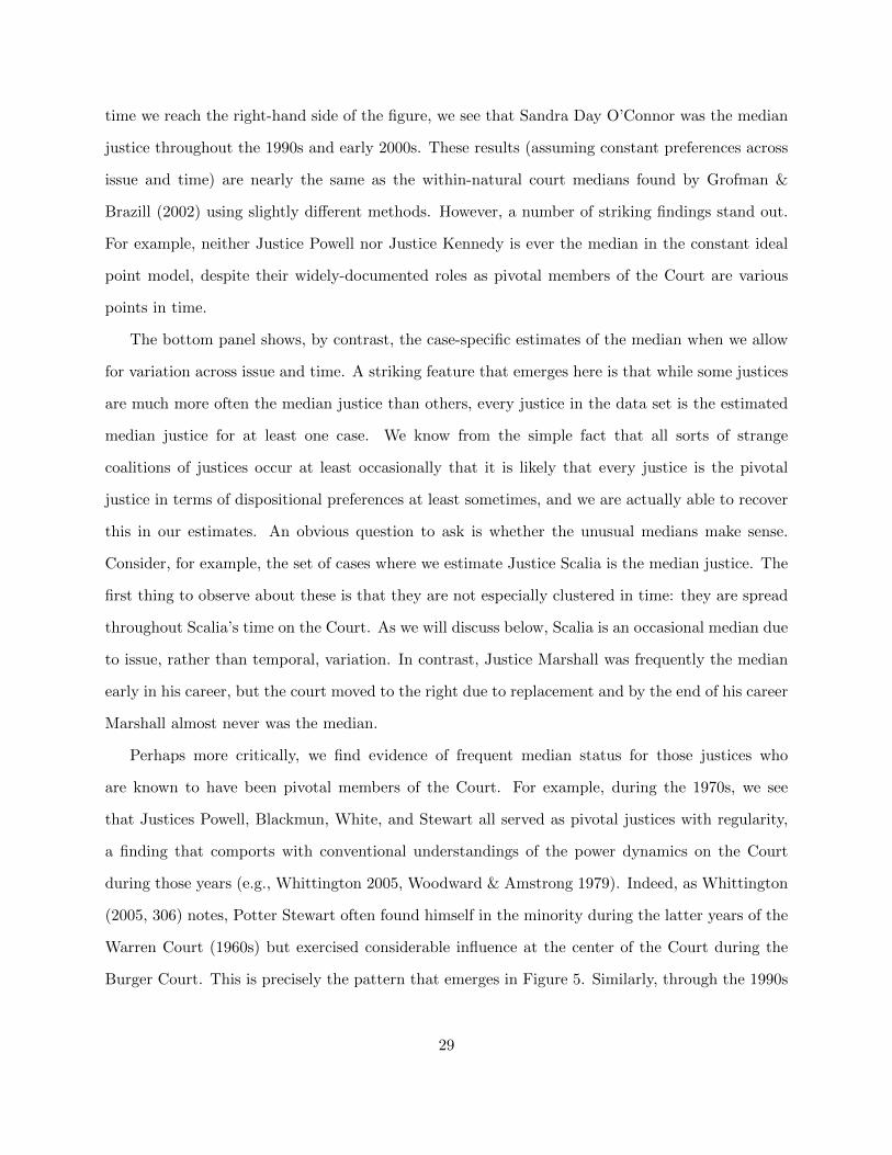
time we reach the right-hand side of the figure, we see that Sandra Day O’Connor was the median

justice throughout the 1990s and early 2000s. These results (assuming constant preferences across

issue and time) are nearly the same as the within-natural court medians found by Grofman &

Brazill (2002) using slightly different methods. However, a number of striking findings stand out.

For example, neither Justice Powell nor Justice Kennedy is ever the median in the constant ideal

point model, despite their widely-documented roles as pivotal members of the Court are various

points in time.

The bottom panel shows, by contrast, the case-specific estimates of the median when we allow

for variation across issue and time. A striking feature that emerges here is that while some justices

are much more often the median justice than others, every justice in the data set is the estimated

median justice for at least one case. We know from the simple fact that all sorts of strange

coalitions of justices occur at least occasionally that it is likely that every justice is the pivotal

justice in terms of dispositional preferences at least sometimes, and we are actually able to recover

this in our estimates. An obvious question to ask is whether the unusual medians make sense.

Consider, for example, the set of cases where we estimate Justice Scalia is the median justice. The

first thing to observe about these is that they are not especially clustered in time: they are spread

throughout Scalia’s time on the Court. As we will discuss below, Scalia is an occasional median due

to issue, rather than temporal, variation. In contrast, Justice Marshall was frequently the median

early in his career, but the court moved to the right due to replacement and by the end of his career

Marshall almost never was the median.

Perhaps more critically, we find evidence of frequent median status for those justices who

are known to have been pivotal members of the Court. For example, during the 1970s, we see

that Justices Powell, Blackmun, White, and Stewart all served as pivotal justices with regularity,

a finding that comports with conventional understandings of the power dynamics on the Court

during those years (e.g., Whittington 2005, Woodward & Amstrong 1979). Indeed, as Whittington

(2005, 306) notes, Potter Stewart often found himself in the minority during the latter years of the

Warren Court (1960s) but exercised considerable influence at the center of the Court during the

Burger Court. This is precisely the pattern that emerges in Figure 5. Similarly, through the 1990s

29

and 2000s, we find Justices O’Connor and Kennedy are both frequently median. Popular observers

of the Court widely noted the way O’Connor and Kennedy shared power during those years (e.g.,

Lane 2006, Lithwick 2006).

Figure 6 shows the frequency of median status for each justice, as a function of issue area instead

of time. Each justice is represented along the y-axis, and each issue area is represented along the

x-axis. For each issue area, the height of the bar indicates the frequency with which he or she was

the median justice in that issue area.

The variation in the identity of the median justice across areas of the law is visible in comparisons

of justices whose tenure on the Court overlapped significantly. Consider again Justices O’Connor

and Kennedy. As we saw in Figure 5, both were regular medians during those years. Which justice

was median depended in part on the issue area of a given case. We see in Figure 6 that Justice

O’Connor was especially likely to be the median in Privacy, Criminal Procedure, Civil Rights,

First Amendment, and Judicial Power Cases. Justice Kennedy, by contrast, was most often the

median in Economic Activity and Federal Taxation cases. Importantly, and as noted above, there is

considerable variation in the extent to which each of these issue areas occupies the Court’s docket.

Federal Taxation and Privacy cases are a very small fraction of the Court’s docket, while Criminal

Procedure, Civil Rights, and First Amendment cases represent a much greater proportion. Indeed,

we see in Figure 6 that Justice O’Connor was more likely to be the median than Justice Kennedy in

the areas with the most cases (those areas to the left end of the x-axis), which is why O’Connor is

identified as the median in analyses that ignore issue variation. At the same time, we also see that

Justices Powell and Blackmun alternated as median justices across issue areas. Justice Powell was

most likely to be the median in Criminal Procedure, First Amendment, and Privacy cases, while

Justice Blackmun was the pivotal member of the Court in Union, Economic Activity, and Judicial

Power cases.

Finally, consider the relatively liberal Justice Breyer and relatively conservative Justice Scalia.

Given their perception as relatively extreme justices, it may have been striking that we found above

in Figure 5 that each of them had been the median justice in at least one case. Though, as we also

see in Figure 5, they are medians in only a small handful of cases, we see in Figure 6 where these

30

Frequency of Median Status by Justice by Issue Area

Crim

inal

Pro

cedu

re

Civ

il R

ight

s

Firs

t Am

endm

ent

Due

Pro

cess

Priv

acy

Atto

rney

s

Uni

ons

Eco

nom

ic A

ctiv

ity

Judi

cial

Pow

er

Fed

eral

ism

Inte

rsta

te R

elat

ions

Fed

eral

Tax

atio

n

Mis

cella

neou

s

Breyer

Ginsburg

Thomas

Souter

Kennedy

Scalia

O'Connor

Stevens

Rehnquist

Powell

Blackmun

Burger

Marshall

Fortas

Goldberg

White

Stewart

Whittaker

Brennan

Harlan

Warren

Minton

Clark

Burton

Jackson

Douglas

Frankfurter

Reed

Black

Figure 6: Frequency of median status, by justice, by issue area. Bars indicate frequency of medianstatus in cases for each justice in each issue areas.

31

justices have had the opportunity to serve as the median. Table 1 lists the 25 cases in which Justice

Scalia is estimated to be the median justice. Interestingly, these cases are concentrated in a few

specific issues. In particular, if Justice Scalia is to be the median justice, it is disproportionately

likely to be in the issue area of Criminal Procedure (15 cases), particularly on the issue of Search

and Seizure (7). Five times, Scalia was the median in Economic Activity cases, four times in Civil

Rights cases, and one in an Attorneys case. Many of these cases occur early in Scalia’s tenure,

before a rightward drift through the 1990s and the appointment of more liberal justices Souter,

Ginsburg, and Breyer. However, throughout the 1990s and early 2000s, Scalia has been pivotal

in Criminal Procedure and Economic Activity cases. In the even rarer instances where Justice

Breyer has had the opportunity to serve as the median, it has been in cases involving the First

Amendment. Indeed, Justice Breyer is known to be more conservative (and thus closer to the

center of the Court) in cases involving freedom of speech than other areas of the law. For example,

we estimate Justice Breyer to be the median justice in Turner Broadcasting v. FCC (1997), a 5-4

case in which he joined Chief Justice Rehnquist and Justices Kennedy, Stevens, and Souter in the

majority, but wrote his own concurring opinion that hinted he was sympathetic to the dissenters’

positions on some issues.

In sum, the cross-issue variation in the identity of the median justice comports with conventional

understandings of the justices’ varying influence across areas of the law. However, our analysis also

yields results that were not anticipated, such as the finding that every justice has served as the

pivotal voter at least once. The substantial and measurable variation in the identity of the median

justice across contemporaneous cases implications for several theoretical and empirical puzzles in

the judicial politics literature.

5. IMPLICATIONS

The preceding analysis demonstrates that the estimation approach we have advanced can recover

well-documented patterns in judicial preferences that were previously not capable of being studied

systematically. What is more, the analysis also documents new, systematic patterns in which

32

Case

Nam

eY

ear

Issu

eA

rea

Issu

e

Mary

lan

dv.

Gar

riso

n198

7C

rim

inal

Pro

ced

ure

Sea

rch

and

seiz

ure

U.S

.v.

Du

nn

1987

Cri

min

alP

roce

du

reS

earc

han

dse

izu

reO

’Con

nor

v.

Ort

ega

1987

Cri

min

alP

roce

du

reS

earc

han

dse

izu

reC

TS

Corp

.v.

Dyn

am

ics

Cor-

pora

tion

198

7E

con

omic

Act

ivit

yS

tate

regu

lati

on,

esp

.of

bu

sin

ess

Ric

har

dso

nv.

Mar

sh198

7C

rim

inal

Pro

ced

ure

Con

fron

tati

onN

ewY

ork

v.

Bu

rger

1987

Cri

min

alP

roce

du

reS

earc

han

dse

izu

reF

razi

erv.

Hee

be

1987

Civ

ilR

ights

Res

iden

cyre

qu

irem

ents

Gri

ffin

v.

Wis

con

sin

1987

Cri

min

alP

roce

du

reS

earc

han

dse

izu

reG

reer

v.

Mil

ler

198

7C

rim

inal

Pro

ced

ure

Mir

and

aw

arn

ings

Pen

nsy

lvan

iav.

Del

awar

eV

all

eyC

itiz

ens’

Cou

nci

l198

7A

ttor

ney

sA

ttor

ney

s’fe

es

Cali

forn

iav.

Gre

enw

ood

1988

Cri

min

alP

roce

du

reS

earc

han

dse

izu

reC

ity

of

Can

ton

v.

Harr

is19

89

Civ

ilR

ights

Des

egre

gati

on(o

ther

than

sch

ool

s)G

rad

yv.

Corb

in199

0C

rim

inal

Pro

ced

ure

Dou

ble

jeop

ard

yU

.S.

v.

Mon

talv

o-M

uri

llo

1990

Cri

min

alP

roce

du

reS

tatu

tory

con

stru

ctio

nof

crim

inal

law

sP

aci

fic

Mu

tualL

ife

v.

Cle

op

a-tr

aH

asli

p199

1E

con

omic

Act

ivit

yL

iab

ilit

y,p

un

itiv

ed

amag

es

Wya

ttv.

Cole

1992

Civ

ilR

ights

Lia

bil

ity,

civil

righ

tsU

.S.

v.

Gra

nd

erso

n19

94

Cri

min

alP

roce

du

reS

tatu

tory

con

stru

ctio

nof

crim

inal

law

sB

arc

lay’s

v.

Fra

nch

ise

Tax

Boar

d199

4E

con

omic

Act

ivit

yS

tate

tax

Lib

rett

iv.

U.S

.199

5C

rim

inal

Pro

ced

ure

Fed

eral

rule

sof

crim

inal

pro

ced

ure

Min

nes

ota

v.

Cart

er1998

Cri

min

alP

roce

du

reS

earc

han

dse

izu

reH

ills

ide

Dair

yv.

Lyo

ns

200

3E

con

omic

Act

ivit

yS

tate

regu

lati

on,

esp

.of

bu

sin

ess

Gen

eral

Dyn

am

ics

v.

Cli

ne

2004

Civ

ilR

ights

Em

plo

ym

ent

dis

crim

inat

ion

(oth

erth

ange

nd

erd

iscr

imin

atio

n)

Sch

riro

v.

Su

mm

erli

n2004

Cri

min

alP

roce

du

reR

etro

acti

vit

yU

.S.

v.

Booker

2005

Cri

min

alP

roce

du

reSta

tuto

ryco

nst

ruct

ion

ofcr

imin

alla

ws

Gra

nh

olm

v.

Hea

ld200

5E

con

omic

Act

ivit

ySta

tere

gula

tion

,es

p.

ofb

usi

nes

s

Tab

le1:

Case

sin

whic

hou

rB

est

Mod

eles

tim

ate

sS

cali

ato

beth

em

edia

nju

stic

e.T

able

show

sn

ames

ofca

ses,

the

year

sth

eca

ses

wer

ed

ecid

ed,

the

Sp

aeth

Issu

eA

rea

assi

gned

toth

eca

se,

and

the

Sp

aeth

Issu

eas

sign

edto

the

case

.

33

preferences vary across areas of the law and over time. However, our analysis has still further a

series of implications for previously unexplored elements of judicial decision-making and power.

Perhaps most critically, the analysis reveals that judicial preferences are simultaneously systematic

and predictable but also variable across substantive areas of the law. In other words, to repeat

from above, judicial preferences over law and legal doctrine cannot be succinctly represented as

simple left-right ideology. While some contemporary research on rule-making in the courts has

been concerned with the theoretical problems associated with multidimensionality within a case

(e.g., Lax 2007), our analysis reveals that judicial politics is both dynamic and multidimensional

across cases. This insight opens the door to a number of previously unexplored features of judicial

power and provides an invitation for new kinds of theorizing.

Nominations and Confirmations. Among the substantive problems for which our analysis

has implications, the most direct is the politics of Supreme Court nominations and confirmations.

While the subject of Supreme Court nominations and confirmations has received a great deal of

attention, one of the fundamental findings that permeates all such studies is that modern Supreme

Court confirmation decisions are largely shaped by anticipations about what the nominees’ policy

views are and, by implication, what affect they will have on the Court’s ideological orientation

(e.g., Cameron, Cover & Segal 1990, Caldeira & Wright 1998, Kastellec, Lax & Phillips 2010). Our

analysis sheds new light on the dynamics of this process and raises theoretical nuance that has not

previously been treated in the literature. For example, because of the primacy of the median justice

for the Court’s decision-making, the stakes of a given Supreme Court nomination may be thought

to hinge on the effect that the nomination will have on the location of the median (Krehbiel 2007).

However, our analysis reveals that any given nomination can do more (or less) than simply move

a median—a nomination may move a median in a small or large number of cases; it may collapse

power from a set of medians into a single median; it may spread power from a concentrated median

to a diffuse set of medians. As a consequence, there are more complicated dynamics involved in

the selection and confirmation of a Supreme Court nominee than simply whether he or she is to

the left or right of the current median. For example, when Justice Stewart, who was one of the

three or four different medians towards the end of his tenure, was replaced with Justice O’Connor,

34

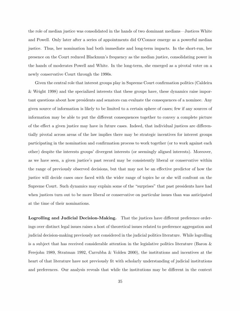
the role of median justice was consolidated in the hands of two dominant medians—Justices White

and Powell. Only later after a series of appointments did O’Connor emerge as a powerful median

justice. Thus, her nomination had both immediate and long-term impacts. In the short-run, her

presence on the Court reduced Blackmun’s frequency as the median justice, consolidating power in

the hands of moderates Powell and White. In the long-term, she emerged as a pivotal voter on a

newly conservative Court through the 1990s.

Given the central role that interest groups play in Supreme Court confirmation politics (Caldeira

& Wright 1998) and the specialized interests that these groups have, these dynamics raise impor-

tant questions about how presidents and senators can evaluate the consequences of a nominee. Any

given source of information is likely to be limited to a certain sphere of cases; few if any sources of

information may be able to put the different consequences together to convey a complete picture

of the effect a given justice may have in future cases. Indeed, that individual justices are differen-

tially pivotal across areas of the law implies there may be strategic incentives for interest groups

participating in the nomination and confirmation process to work together (or to work against each

other) despite the interests groups’ divergent interests (or seemingly aligned interests). Moreover,

as we have seen, a given justice’s past record may be consistently liberal or conservative within

the range of previously observed decisions, but that may not be an effective predictor of how the

justice will decide cases once faced with the wider range of topics he or she will confront on the

Supreme Court. Such dynamics may explain some of the “surprises” that past presidents have had

when justices turn out to be more liberal or conservative on particular issues than was anticipated

at the time of their nominations.

Logrolling and Judicial Decision-Making. That the justices have different preference order-

ings over distinct legal issues raises a host of theoretical issues related to preference aggregation and

judicial decision-making previously not considered in the judicial politics literature. While logrolling

is a subject that has received considerable attention in the legislative politics literature (Baron &

Ferejohn 1989, Stratman 1992, Carrubba & Volden 2000), the institutions and incentives at the

heart of that literature have not previously fit with scholarly understanding of judicial institutions

and preferences. Our analysis reveals that while the institutions may be different in the context

35

of courts, judicial preferences are heterogeneous across topics in predictable ways, allowing for the

possibility of more complicated bargaining dynamics. While the Court does not operate in such a

way that might allow for explicit vote-trading or logrolling (i.e., cases are not decided in packages

together, which undermines the ability to credibly commit to a logroll), previously unappreciated

bargaining dynamics may arise given the long-run nature of judicial relationships, the nearly com-

plete control the Court has over which cases to hear, and the institutionally-unconstrained nature

of judicial decision-making.

As a consequence, perhaps one of the most significant implications of our analysis is that it

opens the door to questions about the nature of judicial bargaining that have not been examined in

the literature. When power is spread across many medians, for example, different incentives arise

concerning the choice to hear a case, because the likely outcome of a case is surely a function of the

preferences of whomever finds him- or herself at the center of the Court on that particular case.

By contrast, when power is concentrated in a single, dominant median justice, the politics of case

selection likely become less contentious. We leave it to future scholarship to more directly develop

these theoretical implications; we raise them only to highlight the types of questions that have been

overlooked in light of the past focus on unidimensional understandings of judicial preferences.

Strategic Litigation. A third substantive problem for which our analysis has important impli-

cations is one that remains under-studied in the judicial politics literature. While a great deal of

the qualitative literature on social reform has contemplated how the courts can be used to achieve

policy changes (e.g., Irons 1982, McCann 1994), political scientists have paid less attention to how

policy-motivated litigants can strategically shape their litigation strategies to achieve their goals

through the courts (for a notable exception, see Baird 2007). Nevertheless, the topic of strategic

litigation has been one of interest to economists and economically-oriented lawyers studying lit-

igation (deFigueiredo 2005, Yates & Coggins 2009). The preceding analysis suggests a series of

important lessons for studies of strategic litigation. First, how an issue is framed can affect who

plays a critical role on the Court for a given case. For example, during the 1970s, a case framed

as a Criminal Procedure case would more likely depend on the view of Justice Powell than if it

were framed as a Civil Rights case, in which Justice White would have been the more likely median

36

justice. Similarly, during the 1990s, a strategic litigant bringing a privacy case would have to cater

more to the views of Justice O’Connor than a litigant with a federal taxation case, where Justice

Kennedy was the more likely median. Because special interests seeking social change may have the

choice to bring their issue to the Court in any one of a series of contexts, this information can be

critical to those interests. We expect that future studies of strategic litigation should incorporate

the multidimensional nature of judicial preferences into the framework in which litigants choose

not just which cases to bring but how to bring those cases.

Beyond The Supreme Court. While the tool we have developed here leverages data sources

that are particular to the US Supreme Court, the key to generating judicial rank orderings that

vary across legal issues is the use of some auxiliary information about which votes are most similar.

Because citation is a feature of legal decision-making more generally, our method could be used to

study other courts as well. With comparable sources of information about citation networks, one

could directly apply our model to other multi-member courts including the US Courts of Appeals;

the European Court of Justice; the European Court of Human Rights; or high courts within other

countries, such as the new Supreme Court in the UK. More generally, there is nothing peculiar to

judicial decision-making about our approach: it is the similarity data rather than the method that

is application-specific. Multidimensional kernel-weighted optimal classification is applicable to a

number of other substantive institutions of interest. This is especially valuable for moving beyond

unidimensional study of other small voting chambers, from city councils to the United National

Security Council. Data on the timing of votes is always available, so the task for researchers is to

identify appropriate measures of substantive similarity between votes. These could be the countries

involved in a negotiation, the industry being regulated, or the constitutional power being exercised

by a legislature, to give just a few examples. Methods for computing relative similarity of texts, such

as cosine distance and latent semantic analysis, may be useful in generating appropriate measures

without manual coding from the various documents that often accompany voting decisions.

37

6. CONCLUSIONS

Nearly all empirical analyses of American political institutions implicate the underlying policy

preferences of political actors. In the context of judicial politics, for example, that judges are

motivated by their policy goals is a finding that first caused considerable controversy within the

subfield and now occupies a place as a virtually unassailable stylized fact. Perhaps as a consequence

of the ubiquity of individual policy preferences in institutional theories of politics, the measurement

of those preferences has emerged as a vibrant and exciting component of contemporary research in

political science. Much of that research has come to be dominated by the use of powerful empirical

tools for measuring latent political spaces. Among the tools employed to measure these spaces,

item-response theory models have become particularly prevalent. However, there are applications

where existing item-response models have severe limitations, and describing variation beyond a

single dimension in an institution with few voters is one of those applications.

By reformulating the problem of describing how preferences vary across issues, we have proposed

an alternative approach that mitigates some of the theoretical and practical limitations of IRT

models. Perhaps most important, the technique we have developed allows us to investigate how

judicial preferences vary across both areas of the law and over time. Our approach allows us to

demonstrate that there is much more to Supreme Court justices’ dispositional voting behavior than

a single left-right political dimension that applies to all legal issues. Justices’ vary in their expressed

doctrine across areas of the law in ways that we can understand and characterize.

Moreover, beyond opening the doors to the new lines of inquiry described above, the case-specific

rank orderings for justices that we recover can facilitate a number of substantive lines of inquiry in

judicial politics. Three such examples, in our view, are as follows. First, powerful theories of rule-

making on the Supreme Court have contemplated how different preference orderings across different

legal dimensions affects the Court’s doctrine (e.g., Lax 2007, Lax & Cameron 2007, Bonneau,

Hammond, Maltzman & Wahlbeck 2007). Our model allows scholars to identify how preference

orderings vary from case-to-case. Indeed, while virtually all theories of bargaining on the Court

assume a unidimensional policy preference structure in the context of an individual decision, none

38

assumes that that dimension or ordering is the same from case-to-case. When examining bargaining

over decisions at the Supreme Court, scholars can make use of our case-specific preference ordering

to evaluate those formal models.

Second, and related, our method allows scholars to investigate the extent to which power is

shared among justices at any given time. Figure 5, for example, shows that during the last 20

years, Justices O’Connor and Kennedy essentially shared power as the median justice of the Court.

By contrast, between 1970 and 1980, more justices were frequently pivotal, with Powell, Blackmun,

White and Stewart holding median status in many cases. Previous research has been concerned

with the relative influence that various median justices exercise (Epstein & Jacobi 2008), but those

studies have been limited by their inability to identify variation in the median across contempora-

neous cases.

A third example concerns the study of compliance in the judicial hierarchy. The study of

compliance often asks whether lower court judges comply with the preferences of superior courts

(e.g., Cameron, Segal & Songer 2000). That empirical exercise requires the analyst to estimate

the “preferences of the Court”; usually, the median justice serves as a stand-in for the Court as a

whole (e.g., Cameron, Segal & Songer 2000, Clark 2009, Westerland, Segal, Epstein, Cameron &

Comparato 2010). Using our methodology, scholars can now capture more nuance and subtlety in

judicial preferences than previous measures made possible—namely variation in judicial preferences

across time and areas of the law.

While we have developed our method in the context of judicial decision-making, our estimation

approach is also applicable, with suitable modifications to address computational issues, to the

study of legislative voting. For example, applications of our method to the legislative context

might make use of many potential measures of which roll call votes are most closely related—

committee of origin, procedural status, the texts of the proposals themselves—that each provide

information about which votes are on substantively similar issues. Such an approach would be

useful for characterizing how legislators’ behavior varies across different kinds of bills, just as in

this paper it provided a useful way of characterizing how judges’ behavior varied across different

kinds of cases.

39

Finally, while the method developed in this paper represents a powerful advance over past

techniques, there is more work to be done. Future research can, and should, develop a probability

model that can capture the kinds of issue variation in preferences that we observe while facilitating

characterizations of estimation uncertainty that are not compatible with our approach. While

the problems of estimating cardinal, inter-temporally comparable remain, methods that combine

varying preferences across time and issue with anchoring data like that of Bailey (2007) would help

ameliorate such concerns. Such techniques could also be applied to courts at different levels of the

judicial hierarchy, generating comparable estimates for the entire U.S. federal Court system. In

this paper, we have demonstrated that there is meaningful, recoverable variation in Supreme Court

justices’ preferences across issues, and we expect this information will provide fruitful groundwork

on which these types of endeavors can build.

REFERENCES

Alfano, Sean. 2009. “The Kennedy Court.”.

URL: http://www.cbsnews.com/stories/2006/07/04/opinion/courtwatch/main1774288.shtml

Bailey, Michael A. 2007. “Comparable Preference Estimates across Time and Institutions for the

Court, Congress, and Presidency.” American Journal of Political Science 51(3):433–448.

Bailey, Michael A. & Forrest Maltzman. 2008. “Does Legal Doctrine Matter? Unpacking Law and

Ideology on the U.S. Supreme Court.” American Political Science Review 102(3):369–384.

Baird, Vanessa A. 2007. Answering the Call of the Court: How Justices and Litigants Set the

Supreme Court Agenda. Charlottesville: University of Virginia Press.

Baron, David P. & John F. Ferejohn. 1989. “Bargaining in Legislatures.” American Political Science

Review 83(4):1181–1206.

Bonica, Adam. 2010. A Day by Day Measure of Legislator Ideology PhD thesis New York University.

40

Bonneau, Chris W., Thomas H. Hammond, Forrest Maltzman & Paul J. Wahlbeck. 2007. “Agenda

Control, the Median Justice, and the Majority Opinion on the U.S. Supreme Court.” American

Journal of Political Science 51(4):890–905. Forthcoming.

Caldeira, Gregory A. & John R. Wright. 1998. “Lobbying for Justice: Organized Interests, Supreme

Court Nominations, and the United States Senate.” American Journal of Political Science

42(2):499–523.

Cameron, Charles M., Albert D. Cover & Jeffrey A. Segal. 1990. “Senate Voting on Supreme Court

Nominees: A Neoinstitutionalist Model.” American Political Science Review 84(2):525–534.

Cameron, Charles M., Jeffrey A. Segal & Donald R. Songer. 2000. “Strategic Auditing in a Political

Hierarchy: An Informational Model of the Supreme Court’s Certiorari Decisions.” American

Political Science Review 94:101–16.

Carrubba, Clifford J. & Craig Volden. 2000. “Coalitional Politics and Logrolling in Legislative

Institutions.” American Journal of Political Science 44(2):261–277.

Clark, Tom S. 2009. “A Principal-Agent Model of En Banc Review.” Journal of Law, Economics

& Organization 25(1):55–79.

Clark, Tom S. & Benjamin Lauderdale. 2010. “Locating Supreme Court Opinions in Doctrine

Space.” American Journal of Political Science 54(4):871–890.

Clinton, Joshua D. & Adam Meirowitz. 2003. “Integrating Roll Call Analysis and Voting Theory:

A Framework.” Political Analysis 11:381–396.

Clinton, Joshua D., Simon Jackman & Douglas Rivers. 2004. “The Statistical Analysis of Roll Call

Data.” American Political Science Review 98(2):355–370.

Cole, David. 2006. “The ‘Kennedy Court’.”.

deFigueiredo, John M. 2005. “Strategic Plaintiffs and Ideological Judges in Telecommunications

Litigation.” Journal of Law, Economics & Organization 21(2):501–523.

41

Eddelbuettel, Dirk & Romain Francois. 2011. “Rcpp: Seamless R and C++ Integration.” Journal

of Statistical Software 40(8):1–18.

URL: http://www.jstatsoft.org/v40/i08/

Epstein, Lee & Tonja Jacobi. 2008. “Super Medians.” Stanford Law Review 61:37–100.

Greenhouse, Linda. 2005. Becoming Justice Blackmun: Harry Blackmun’s Supreme Court Journey.

New York: Times Books.

Greenhouse, Linda. 2010. “Is the ‘Kennedy Court’ Over?”.

URL: optinionator.blogs.nytimes.com/2010/07/15/rethinking-the-kennedy-court

Grofman, Bernard & Timothy J. Brazill. 2002. “Identifying the Median Justice on the Supreme

Court through Multidimensional Scaling: Analysis of “Natural Courts” 1953-1991.” Public

Choice 112(1/2):55–79.

Ho, Daniel E. & Kevin M. Quinn. 2010. “How Not to Lie with Judicial Votes: Misconceptions,

Measurement, and Models.” California Law Review 98(3):813–876.

Irons, Peter H. 1982. The New Deal Lawyers. Princeton University Press.

Jeffries, Jr., John C. 1994. Justice Lewis F. Powell, Jr.: A Biography. Fordham University Press.

Jessee, Stephen. 2009. “Spatial Voting in the 2004 Presidential Election.” American Political

Science Review 103:59–81.

Kastellec, Jonathan P., Jeffrey R. Lax & Justin H. Phillips. 2010. “Public Opinion and Senate

Confirmation of Supreme Court Nominees.” Journal of Politics 72(3):767–784.

Krehbiel, Keith. 2007. “Supreme Court Appointments as a Move-the-Median Game.” American

Journal of Political Science 51(2):231–240.

Lane, Charles. 2006. “Kennedy Reigns Supreme on Court.” Washington Post July 2, 2006.

Lax, Jeffrey R. 2007. “Constructing Legal Rules on Appellate Courts.” American Political Science

Review 101(3):591–604.

42

Lax, Jeffrey R. 2011. “The New Judicial Politics of Legal Doctrine.” Annual Review of Political

Science 14:131–157.

Lax, Jeffrey R. & Charles M. Cameron. 2007. “Bargaining and Opinion Assignment on the U.S.

Supreme Court.” Journal of Law, Economics, and Organization 23(2):276–302.

Lithwick, Dahlia. 2006. “Swing Time.”.

URL: http://www.slate.com/id/2134421/

Londregan, John. 2000a. “Estimating Legislators’ Preferred Points.” Political Analysis 8(1):35–56.

Londregan, John. 2000b. Legislative Institutions and Ideology in Chile. Cambridge University Press.

Martin, Andrew D. & Kevin M. Quinn. 2002. “Dynamic Ideal Point Estimation via Markov Chain

Monte Carlo for the U.S. Supreme Court, 1953-1999.” Political Analysis 10:134–153.

Martin, Andrew D., Kevin M. Quinn & Lee Epstein. 2005. “The Median Justice on the U.S.

Supreme Court.” North Carolina Law Review 83(5):1275–1322.

McCann, Michael W. 1994. Rights at Work. University of Chicago Press.

Moraski, Byron J. & Charles R. Shipan. 1999. “The Politics of Supreme Court Nominations:

A Theory of Institutional Constraints and Choices.” American Journal of Political Science

43(4):1069–1095.

Newman, Roger K. 1997. Hugo Black: A Biography. New York: Fordham University Press.

Peress, Michael. 2009. “Small Chamber Ideal Point Estimation.” Political Analysis 17:276–290.

Plott, Charles R. 1967. “A Notion of Equilibrium and Its Possibility Under Majority Rule.” Amer-

ican Economic Review 57:787–806.

Poole, Keith T. 2000. “Nonparametric Unfolding of Binary Choice Data.” Political Analysis

8(2):211–237.

Poole, Keith T. 2005. Spatial Models of Parliamentary Voting. Cambridge University Press.

43

Poole, Keith T. & Howard Rosenthal. 1997. Congress: A Political-Economic History of Roll Call

Voting. Oxford University Press.

R Development Core Team. 2008. R: A Language and Environment for Statistical Computing.

Vienna, Austria: R Foundation for Statistical Computing.

Segal, Jeffrey A. & Harold J. Spaeth. 2002. The Supreme Court and the Attitudinal Model Revisited.

Cambridge University Press.

Spaeth, Harold, Lee Epstein, Ted Ruger, Keith Whittington, Jeffrey Segal & Andrew D. Martin.

N.d. “The Supreme Court Database.”.

Spriggs, II, James F. & Thomas G. Hansford. 2002. “The U.S. Supreme Court’s Incorporation and

Interpretation of Precedent.” Law & Society Review 32(1):139–159.

Stephenson, Karen & Marvin Zelen. 1989. “Rethinking Centrality: Methods and Examples.” Social

Networks 11:1–37.

Stern, Seth & Stephen Wermiel. 2010. Justice Brennan: Liberal Champion. Houghton Mifflin

Harcourt.

Stratman, Thomas. 1992. “The Effects of Logrolling on Congressional Voting.” American Economic

Review 82(5):1162–1176.

Tahk, Alexander M. 2006. “A New Approach to Optimal Classification.” Annual Meeting of the

American Political Science Association .

Wasserman, Larry. 2005. All of Nonparametric Statistics. Springer.

Westerland, Chad, Jeffrey A. Segal, Lee Epstein, Charles M. Cameron & Scott Comparato. 2010.

“Strategic Defiance and Compliance in the U.S. Courts of Appeals.” American Journal of

Political Science 54:891–905.

Whittington, Keith E. 2005. The Burger Court, 1969-1986: Once More in Transition. In The United

States Supreme Court: The Pursuit of Justice, ed. Christopher Tomlins. Boston: Houghton

Mifflin pp. 300–322.

44

Woodward, Bob & Scott Amstrong. 1979. The Brethren. Simon & Schuster.

Yates, Jeff L. & Elizabeth Coggins. 2009. “The Intersection of Judicial Attitudes and Litigant

Seleciton Theories: Explaining U.S. Supreme Court Decision Making.” Washington University

Journal of Law and Policy 29(1):263–299.

Zucco, Jr., Cesar & Benjamin E. Lauderdale. 2011. “Distinguishing Between Influences on Brazilian

Legislative Behavior.” Legislative Studies Quarterly .

45

the supreme court’s many median...

Documents