the strategic interaction between committing and … the strategic interaction between committing...
TRANSCRIPT

1
The Strategic Interaction between Committing and Detecting
Fraudulent Misreporting*
Buhui Qiu; Steve L. Slezak
ABSTRACT
The paper considers an agency model of fraudulent misreporting which implies a rich set of
relationships between the commission of fraud, the observation or detection of fraud, economic
performance, and the compensation policy of the firm. The paper develops a number of testable
empirical implications and highlights several interesting phenomena, including implications on
exogenous variables that can cause an increase in the amount of fraud committed but a decrease
in the amount of fraud being observed (and visa versa). Thus, empirical studies that seek to
identify the firm or managerial characteristics associated with the commission of fraud cannot
infer a relationship by simply examining how the amount of observed fraud varies with these
characteristics. In addition, the paper also shows that an increase in an industry’s growth
potential can cause that industry to fall from a high-productivity pooling equilibrium (with high
levels of incentive compensation and effort and, as a result, many high-productivity firms) to the
lower-productivity mixed-strategy equilibrium (with lower levels of incentive compensation and
effort and, as a result, fewer high-productivity firms), resulting in a drop in economic
performance.
* Buhui Qiu (who will attend the meeting and present the paper) is assistant professor in finance from Rotterdam School of Management Erasmus University, Burgemeester Oudlaan 50, 3062 PA Rotterdam, The Netherlands (Tel:31-10-4088520; Fax: 31-10-4089017; E-mail: [email protected]). Steve Slezak is associate professor in finance from College of Business, University of Cincinnati, Cincinnati, Ohio 45221, USA (Tel: 1-513-5567023; Fax: 1-513-5564891; Email: [email protected]). We thank Sandra Betton, Mathijs van Dijk , Alan Douglas, Mike Ferguson, Hui Guo, Young Koan Kwon, Albert (Pete) Kyle (FMA doctoral seminar session chair), Gregory Lipny, Carolina Salva, Raj Singh (WFA discussant), Weihong Song, James Thomson, Marno Verbeek, Kenneth Vetzal, Tracy Wang, seminar participants at Concordia University (Montreal), Rotterdam School of Management (Erasmus University), Singapore Management University, the University of Cincinnati, the University of Waterloo, and Vlerick Leuven Gent Management School, session participants at the 2008 Western Finance Association annual meeting in Waikoloa, Hawaii, session participants at the 2008 Finance Management Association annual meeting and FMA doctoral seminar in Dallas, Texas, and session participants at the 14th Conference on the Theories and Practices of Securities and Financial Markets (SFM) in Kaohsiung, Taiwan for helpful comments and suggestions. Qiu also gratefully acknowledges the financial support from the 14th SFM conference through their Taiwan Stock Exchange best paper award for an earlier version of the paper. This paper is the first chapter from Buhui Qiu’s doctoral dissertation. All errors are ours.

2
1. Introduction
The revelation of fraudulent misreporting in numerous high-profile cases in the United
States around the start of the twenty-first century (e.g., Adelphia, Enron, Global Crossing, Tyco,
Waste Management Inc., and Sunbeam) resulted in a substantial loss in market value.1 It is
unclear, however, whether these cases represent isolated instances of lapses in corporate ethical
judgment or whether they indicate a general degradation in corporate morality and/or an increase
in the incentive to commit fraud. Clearly indicating a belief in a systemic source, the U.S.
Congress enacted the Sarbanes-Oxley Act in 2002 in an effort to rein in managers in what was
feared to be a pervasive “fast and loose with the facts” opportunistic corporate culture. Yet, it is
still unclear what social or economic forces changed to cause the increase in fraudulent
misreporting. In addition, without knowing the cause, it is also unclear whether
Sarbanes-Oxley will be an effective counter-measure (especially given the time-series and
cross-sectional variation in the economic conditions firms face). In fact, the recent arrests of
two Bear Sterns hedge fund managers and the Securities and Exchange Commission
investigations of dozens of corporate fraud cases related to sub-prime mortgage securities would
seem to raise doubt.
The above issues are difficult to address because the amount of fraud committed is not
directly observable; we only observe the amount of fraud that is detected, which is jointly
determined by the amount of fraud actually being committed and the probability of getting
caught given the extent to which fraudulent activities are investigated. To the extent that
environmental influences may affect the commission and investigation of fraud differently, there
1 According to Cornerstone Research, 231 fraud lawsuits in the year 2002 alone resulted in a total disclosed dollar loss of $203 billion in market capitalization. From 1996 to 2004, on average there were 195 lawsuits per year with a total disclosed dollar loss of $127 billion per year; typically around 80% of these lawsuits involve misrepresentation of financial statements. When looking into these misrepresentation cases, one can find that almost all of them involve earning inflation of some sort.

3
may not be a one-to-one correspondence between the amount of fraud observed and the amount
committed. Thus, the fact that fraudulent behavior is not observable makes it difficult to
discover and document links between potential environmental influences and fraudulent behavior.
Instead, we must develop theoretical models which provide testable implications with respect to
observable phenomena and, when these models are supported by the data, infer relationships
among non-observable variables based on the implications of such models. In order to provide
such structure, this paper develops a theoretical model of fraud with two critical features: (1)
there is a strategic interaction between the commission and detection of fraud (which allows us
to develop conditional statements on what can and cannot be inferred about the commission of
fraud from the observation of fraud), and (2) the extent of fraud committed and investigated
varies with the economic environment (which allows us to develop time-series and
cross-sectional implications on the amount of fraud and the effectiveness of regulation).
Specifically, we develop an agency model in which managers are induced via an
equity-based compensation (EBC) contract to exert personally costly effort that increases the
expected returns of the firm. In the model, the realized return of the firm is not observable by
the market; rather the manager must report its value. Similar to Goldman and Slezak (2006),
EBC provides the manager the incentive to exert effort – but also the incentive to upwardly bias
reports. The regulatory agency, seeking to minimize the deadweight loss associated with fraud,
is responsible for detecting fraud and imposing penalties; it bases its investigation strategy on the
manager’s equilibrium fraud commission strategy in order to optimally trade off the benefit of
reducing fraud against the agency’s detection cost.
To capture both cross-sectional and time-series variation (high growth versus
old-economy firms and recession versus expansion), we assume that after the initial stage, a

4
potential new investment project arrives with a certain probability (proxying for growth
potential). After privately observing the project’s expected profitability, the manager either
adopts or rejects it. In order to obscure past fraud, fraudulent managers have the incentive to
over-invest (i.e., invest in new projects that have negative expected NPV). This
overinvestment results in the deadweight loss associated with fraud.2
Depending upon the parameters characterizing the regulatory and contracting
environment, three potential types of equilibrium may obtain: truthful separating equilibrium in
which each manager truthfully reports their realized return, pooling equilibrium in which all
poorly-performing managers mimic the reports of highly-performing managers but the regulatory
agency does not monitor to verify reports, and a mixed strategy equilibrium in which
poorly-performing managers commit fraud with an equilibrium probability while the regulatory
agency randomly audits those firms that report high earnings.
The paper provides a number of empirical implications regarding the commission and
detection of fraud, incentive contracts, and economic performance. First, the model implies
that fraudulent reporting activities will be concentrated in high-growth industries. This result is
similar to the theory predictions of Wang (2006) and consistent with the empirical evidence in
Wang (2005) and Johnson, Ryan and Tian (2003).3 Second, the model implies that while the
fraud incentive is strongest in good times, fraud commission and detection are more likely to
2 The exact nature of the deadweight loss is not critical for most of our results; all that is needed is that there be some benefit to reducing fraud (in terms of more efficient production) so that the regulator must balance the benefit of reduced fraud against the implementation costs associated with monitoring fraud. However, the paper does develop some implications related to the specific form of fraud inefficiency we assume. 3 Wang (2005) provides empirical evidence that firms engaging in fraudulent reporting tend to overinvest relative to their peers. Johnson, Ryan and Tian (2003) find that their sample of exposed fraudulent reporting firms are not random draws from all possible industries, but rather demonstrates a statistically significant industry concentration, with the concentrated industries having significantly higher than average growth potential.

5
occur when the high growth industries fall into downturns.4 Specifically, when the parameters
are such that the pooling equilibrium obtains, then there will be relatively high levels of EBC,
high average short-term performance, and no fraud being exposed (although fraud is committed).
In contrast, when the parameters are such that the mixed strategy equilibrium obtains, the
equilibrium will have low EBC, low average short-term performance, and fraud will be exposed.
Thus, consistent with the empirical evidence in Johnson, Ryan and Tian (2003), these results
imply that exposed fraud will occur in periods with relatively weak economic performance.5
Third, the model implies that an increase in growth potential, which is typically good
news (i.e., implies higher future profitability and, as a result, increased firm value), can strikingly
have a negative impact on value and economic performance. Specifically, we show that, by
altering the incentives to commit and investigate fraud, an increase in growth potential alone can
cause an industry to fall from a high-productivity pooling equilibrium (with high levels of EBC
and effort and, as a result, many high-productivity firms) to the lower-productivity
mixed-strategy equilibrium (with lower levels of EBC and effort and, as a result, fewer
high-productivity firms), resulting in a drop in economic performance. We show that, given the
strategic interaction between the incentives to commit and investigate fraud, this drop in
economic performance will be accompanied by an increase in the amount of exposed fraud.
These results imply that, while innovation may be beneficial to economic growth by generating
increased future growth opportunities, innovation can also have a dark side when fraud is
possible. In fact, there are many examples of innovations that were accompanied by fraud
scandals: financial innovation in mortgage derivatives, product innovation in
4 Its primary focus, the model in Povel, Singh, and Winton (2007) generates similar “boom-and-bust” results. As discussed below, the two models and the mechanisms by which these boom-and-bust results obtain differ. 5 Their results show that both the exposed fraud firms and their (industry- and size-matched) control firms significantly underperformed the overall stock market during the fraudulent reporting periods.

6
telecommunications, and innovation created by the deregulation of energy markets, to name a
few.
Fourth, the model implies that the extent of detected fraud need not be indicative of the
extent of fraud committed. This is in contrast to the signal jamming models of fraud (see, for
example, Goldman and Slezak (2006)) in which the equilibrium probability of committing fraud
is one. In these types of models, an increase in the probability of detection will necessarily
result in an increase in the incidence of observed fraud. In our model, however, the equilibrium
probability of committing fraud can be inversely related to the probability of observing detected
fraud (in the mixed strategy equilibrium), leading to potential ambiguity in the statistical
relationship between the amount of fraud detected and committed.
Similar to our model, there is a strategic interaction between the commission and
detection of fraud in Povel, Singh, and Winton (2007), hereafter PSW, and Wang (2006); in both
of these models the extent to which managers are monitored depends upon the information
content of the managers’ equilibrium reports and the extent to which managers commit fraud (i.e.,
bias and reduce the informativeness of reports) depends upon the likelihood of being monitored.
In both models, monitoring serves to reduce adverse selection caused by fraud. In Wang (2006),
managers commit fraud on behalf of current equity holders who benefit from a lower cost of
capital stemming from inflated equity prices caused by fraud. In PSW, managers seek outside
funding for their projects and provide (potentially fraudulent) information on the prospects of
these projects to potential investors who face adverse selection in deciding whether or not to
provide funding. In their model, managers receive non-contractible control benefits from any
(even negative NPV) investment and, as a result, they commit fraud in an effort to mislead
investors into funding negative NPV projects so that they can obtain these benefits of control.

7
In both models, the cost of fraud derives from an over-investment problem similar to Myers and
Majluf (1984).
In contrast to these models, fraud in our model stems from an agency problem between
managers and shareholders, with managers seeking to manipulate prices upward in order to
increase their equity-based compensation. As in Goldman and Slezak (2006), equity-based
compensation is a “double-edged sword” in that it provides both the incentive for the managers
to exert costly effort in improving the profitability of the firm and the incentive to commit fraud.
Given this dual role, the possibility of fraud alters the incentive contract, which alters the
equilibrium level of effort and the productivity of firms. Thus, in contrast to PSW and Wang
(2006), which take the distribution of firm productivity as given and consider how fraud affects
the allocation of resources among the fixed set of firms, our model endogenously determines the
productivity of the set of firms via the incentive contract. In contrast to Goldman and Slezak
(2006), which takes the investigation of the regulatory agent as given, our model considers the
strategic interaction between the regulatory agent and the manager in the context of this agency
problem. We show that this combination of elements generates new insights.
Another key difference between our model and the model in Wang (2006) is that we
consider the behavior of a regulatory agency that is concerned with social welfare.6 In Wang
(2006), the monitor chooses whether or not to investigate by trading off the investigation cost
against the penalties the monitoring agency “earns” when fraud is detected. That is, the
monitor in Wang (2006) seeks to maximize the expected profit from monitoring, with the
penalties -- set exogenously -- representing revenue to the monitor. Thus, since the
6 In PSW, firms are not monitored by a regulatory agency such as the SEC. Rather, the potential investors decide whether or not to investigate the claims of firms further prior to investing. Although there is no regulatory agency in PSW, their potential investors’ decision to investigate depends upon trade-offs that are analogous to those considered by the RA in our model.

8
exogenously set penalty is not tied to the endogenously-determined cost of fraud, the behavior of
the monitor in Wang (2006) is not motivated by social welfare. In contrast, our monitor’s
behavior is motivated by social welfare.7
The remainder of the paper is organized as follows. Section 2 describes the model.
Section 3 discusses the equilibria. Section 4 discusses the empirical implications of the model.
Section 5 concludes. All proofs, as well as a numerical example, are provided in the appendix.
2. The Model
The model consists of a large number of competitive firms (in a variety of different
industries) owned by atomistic risk-neutral investors and managed by risk neutral agents. Every
firm within a given industry has exactly the same characteristics. The sequence of events unfolds
over four periods as following.
2.1. Period 1: The Contracting Stage
In period t = 1, an entrepreneur with an idea starts a firm consisting of real and intellectual
assets whose initial value is normalized to 1. The entrepreneur has limited expertise at managing
the on-going operations of the firm and, thus, hires a wealth-constrained professional manager
from a competitive managerial labor market to manage the firm for her. Because the manager is
wealth constrained, the first-best contracting solution, in which the entrepreneur sells the firm to
the manager, is not feasible. Instead, the entrepreneur offers the manager a compensation
contract ),( αw , where w is a nonnegative fixed wage (paid to the manager at t = 1) and α is
the percentage of the firm’s shares offered to the manager in the form of a stock option with a zero
strike price; the option vests in period t = 2. The manager either accepts or rejects the contract,
7 Both the investors in PSW and the regulatory agency in our model trade off the benefit of reduced over-investment against the investigation cost (which includes the cost of investigating truthful firms). In both models, the deadweight loss associated with fraud-induced resource misallocation and the costs incurred to limit fraud are minimized.

9
based on a comparison of the manager’s expected utility under the contract and his reservation
utility, which for simplicity (and without a loss of generality) is assumed to be zero. Once a
manager has been hired and the terms of the contract are set, the entrepreneur sells her ownership
stake in the firm at an initial public offering. The risk-neutral entrepreneur chooses the contract in
order to maximize her expected wealth, given that the value of the firm will depend, via rational
expectations, on the incentives embodied in the contract and on other features of the market,
especially the regulatory environment and the behavior of the regulatory agency (hereafter referred
to as the RA).
After the manager is hired and the IPO is complete, the manager exerts an unobservable
amount of costly effort e , which affects the return on the firm’s assets realized in period t = 2
(described further in the next section). The manager chooses the amount of effort to exert given
the trade off between its beneficial effect on his compensation (via its effect on firm value) and its
detrimental effect on his utility via a disutility of effort given by 2
2e
δ, where δ is a positive
constant. That is, the manager’s objective function is U(.) = E[W] - 2
2e
δ, where E[W] is his
expected wealth conditional on the contract and the economic/regulatory environment.
2.2. Period 2: The Reporting and Investigating Stage
In period t = 2, the return on the firms initial assets is realized and privately observed by the
manager. For simplicity, we assume that the gross return of the firm is either Ha or
La <Ha .8
The probability that the gross return is Ha is eeP ϕ=)( , where ϕ (i.e., the marginal
8 In the real world, the returns of firms are likely to be continuous. However, all that is required for our results is that the return support be bounded above. If the return distribution is bounded from above, then there is a limit to the amount that higher-type managers can exaggerate their return. As a result, since the higher-type managers will not always report returns exceeding those of lower-type managers (at some point their claims cease to be feasible), there will exist situations in which lower-type managers will pool (with some positive probability) with higher-type managers.
10
productivity of effort) is a positive constant and ]/1,0[ ϕ∈e ; while the probability that the gross
return is La is 1 - )(eP .
Once the manager privately observes the realized return on assets, he must make an
earnings report (denoted r) to the market. Since the realized return is not directly observable by
anyone other than the manager, the manager can chose to either report truthfully or fraudulently.
We assume the manager can either truthfully disclose or inflate his earning. Specifically, a
manager with a realized return Ha reports earning truthfully thus r(
Ha ) = Ha . However, a
manager with a realized return of La may report truthfully (i.e., r( La ) = La ) or fraudulently (i.e.,
r( La ) = Ha ). 9 Given the equilibrium information content of the manager’s equilibrium
reporting strategy, market investors rationally value the firm conditional on the firm’s reported
earnings. The manager then exercises his stock option and sells all his vested shares to the
market.10
The RA, which seeks to protect the interests of investors (including the entrepreneur), is
responsible for investigating and detecting fraud. For simplicity, we assume that if the RA
chooses to investigate fraud, it will always detect fraud when it exists and will never “detect” fraud
when it does not exist. That is, the RA does not make ex-post Type I or Type II errors. In order
9 Since there are only two return values possible, the manager will report either r =Ha or r =
La . Any other
reports will not be credible as other values of r are not feasible. 10 Here we assume the manager has a short horizon. We do this for two reasons. First, there is some evidence that this is consistent with the situations in many real-world fraud cases. (Bergstresser and Philippon (2006) present evidence that CEOs exercise unusually large amount of options during periods of high accruals (which indicate intensive earning manipulation).) Second, it markedly simplifies the analysis without affecting the nature of the results. Even if the manager is given a multi-period contract, as long as he receives some compensation based on intermediate value of the firm, he will still have an (albeit mitigated) incentive to manipulate earnings reports to raise the intermediate price of the firm. In a setting in which the manager receives part of his compensation based on long-term value, the weight placed on long-term value will reduce the incentive to commit fraud and will complement the incentives created by penalties for fraud. Since our model has both incentives (EBC) and disincentives (penalties) to commit fraud, adding an addition disincentive (by placing weight on the terminal value) will not change the nature of our results. See Wang (2006) for an analysis of the case where the manager has a long horizon.

11
to detect fraud, however, the RA must choose to investigate fraud. Thus, a manager who has
committed fraud can “get away with it” if the RA chooses not to investigate the manager’s firm.
We assume that it costs IC > 0 to investigate fraud and that the RA decides whether to
investigate fraud to minimize the deadweight loss associated with fraudulent reporting, taking into
consideration both the expected benefits (i.e., the deterrent effect) and costs associated with its
investigation policy. If the RA detects fraud, the manager is assessed a penalty
)( LHD aaffa −≡ proportional to the extent of the misreporting, where f is the constant of
proportionality.11
2.3. Period 3: The Investment Stage
At t = 3, new investment opportunities may become available. The probability that a new
investment opportunity arrives is λ . For simplicity, all new investment opportunities require an
additional investment of capital equal to I , which is raised by issuing equity. If a new investment
opportunity arrives, its gross return will be εµ + , where µ is the mean of the gross return and ε
is a white-noise term following ),0( 2σN . We assume that the manager privately observes the
realized value of mean µ , but that, with respect to the investors information set, µ is a random
variable distributed as ),( µµUniform with µµ <<< 10 and 1)( ≤µE .12 The white noise
error ε is realized at the end of the economy at t = 4. The distributions of µ and ε are
common knowledge. The manager makes an optimal investment decision to maximize his own
payoff; if he is indifferent between investing and forgoing the project, he will invest in any positive
11 As we will see below, the only type of fraud committed is when the manager reports
Ha when in fact La has
occurred. Thus, the “extent” of the fraud is )( LHD aaa −≡ and f is the marginal penalty. For simplicity,
we do not model the optimal choice of f by the RA.
12 We assume 1)( ≤µE to reflect the fact that it is not easy to find positive NPV projects in the real world.

12
NPV project to maximize the ultimate shareholders’ value.13
2.4. Period 4: The Liquidation Stage
At t = 4, the firm is liquidated and the gross returns from old and (if existing) new projects
are distributed to shareholders. Once the firm is liquidated, the truth in past reports may be
revealed. For example, consider the situation in which there is undetected fraud (i.e., the gross
return was aL, the manager reported aH but the RA did not investigate at t = 2). If there is no new
investment at t = 3, the realized terminal cash flow of the firm, aL, will make it apparent that the
manager committed fraud when he reported aH. The RA has no discretion and has to investigate
such cases. If, however, there is new investment at t = 3, the terminal cash flow will be
La µ ε+ + . As a result, if the new investment is taken, there will be no direct evidence of fraud
since the support of La µ ε+ + overlaps with the support of La µ ε+ + . We assume that if the
cash flow is sufficiently low, such that the probability that the t= 2 gross return was aL is
sufficiently high, then the RA will investigate.14 That is, there is a set critical value K such that if
the terminal cash flow is at or below this critical value, the RA will investigate fraud. Since the
realized cash flow of a non-fraudulent firm may also fall below K, non-fraudulent firms may be
investigated. However, again we assume that the RA does not make any ex-post Type I or Type II
errors once it decides to investigate. That is, if it investigates a fraudulent firm, the manager is
caught and assessed the penalty; if it investigates a non-fraudulent firm, the manager is exonerated
and no penalty is assessed. 13 These assumptions are employed to abstract away from the Myers-Majluf type underinvestment problem associated with high-return firms. These assumptions simplify our model and are consistent with the manager receiving some performance-based compensation based on the overall terminal value of the firm. If we instead assume the manager acts to maximize old shareholder value as is in Myers and Majluf (1984), the fraudulent firm manager will have additional incentive to overinvest (i.e., to exploit the overvaluation of his firm’s stock price). Thus, the nature of our results will be the same. 14 Wang (2006) provides a detailed justification for this behavior by showing how mingling cash flows from multiple projects negatively affects the information content of realized returns with respect to fraud. We adopt a simple abstraction of her model to capture this feature.

13
Given that the RA investigates at t = 4 whenever the reported gross return from new
investment is lower than K , if prior undetected fraud exists and there is new investment at t = 3,
the firm will be investigated if its gross return from the new investment is lower than KI
aD + .
The first term is the difference in the return that the new investment must make up for the final
return to be consistent with the manager’s prior earnings report. The value of K is an addition
term that requires the reported return from new investment to be sufficiently unusual to warrant
investigation. We assume that K is small (K<<1) and its value is set prior to t = 1.15,16 The
investigation cost of the RA is again IC per case.
3. Equilibrium
The model is solved by backward induction. Section 3.1 determines the optimal
investment rule of the manager at t = 3 as a function of the exogenous parameters as well as the
endogenous variables determined prior to t = 3 (i.e., the compensation contract ),( αw and the
manager’s reporting strategy). Section 3.2 derives the optimal reporting and auditing strategies,
anticipating the investment strategy derived in section 3.1 and taking as given the compensation
contract ),( αw . Section 3.3 characterizes the optimal compensation contract ),( αw offered to
15 Since the objective of the RA is to minimize deadweight loss, if the RA chooses K at t = 4, it will set K equal to zero. This is true because (as can be seen in the next section) the only benefit of fraud detection in our model is to prevent the cost associated with over-investment, which, at t = 4, is sunk. Thus, there is no benefit to investigating at t = 4 and, given the positive investigation cost, the optimal amount to investigate is zero. 16 We assume that K is small and exogenously set (rather than endogenously determined) in the model. We do this because there are likely to be many factors outsider the bounds of this model that will affect the setting of K in the real world. For example, in the model, for simplicity we assume that the RA makes no ex-post type I and type II errors, and that the investigation cost is fixed per case. However, in the real world, corporate executives are insiders and understand the complicated businesses of their firms much better than outsiders. When a firm is big and there exist multiple investment projects, it is very difficult for outsiders to distinguish cash flows from different projects of the firm. The investigation and litigation process will become very lengthy and very costly, and ex-post type I and type II errors, which are very costly to stakeholders of the firm, are also possible to be made. Thus, although ideally an optimal K should be set through trading off the expected benefits of deterring fraud and the investigation costs, there will be other important factors outside the boundary of this model that will affect the optimal K, which justifies K to be set exogenously and be small.

14
managers at t = 1, anticipating all of the optimal strategies in the subsequent sub-games. To fully
characterize the equilibrium, Section 3.4 describes the conditions under which a specific type (e.g.,
separating, pooling, or mixed) of equilibrium obtains.
The equilibrium concept we adopt is the rational expectation perfect Bayesian equilibrium
(PBE) characterized by: (a) common belief of the RA and market investors (regarding the
investment behavior of the manager at t = 3, the probability that a firm that reports a high return
is truly an Ha -type firm at t = 2, and the managerial effort choice at t = 1) is reasonable (derived
from the manager’s effort choice and reporting and investing strategies with rational expectation
and using Bayes’ rule whenever possible); and (b) given the reasonable common belief, the effort
choice and reporting strategy of the manager, the evaluation strategy of market investors and the
detecting strategy of the RA are sequentially rational.17
3.1. The Investment Decision of the Manager at t = 3
In the liquidation process (i.e., t = 4) prior undetected fraud (if any) will be investigated
and the fraudulent-reporting ( La -type) manager will be subsequently penalized if either new
investment does not occur at t = 3, or the realized return from new investment is too low (i.e.,
KI
aD +<+ εµ ).
At t = 3, if there is no prior undetected fraud, the manager will invest in the expansion
opportunity when 1≥µ . That is, a non-fraudulent manager only invests in opportunities with an
expected NPV greater than or equal to zero. If there is prior undetected fraud, however, the
manager will rationally invest in any project (even a negative expected NPV project) that arrives.
17 The PBE concept here should be equivalent to the sequential equilibrium concept of Kreps and Wilson (1982) since there are only two types of firms in the model – the sequential equilibrium concept will be stronger if the types of firms are more than two. See Fudenberg and Tirole (1991) for a proof.

15
Thus, fraud causes an overinvestment problem. 18 The reason for this overinvestment is
straightforward. If the manager does not invest in the expansion opportunity, evidence of his
prior fraud will be exposed in liquidation and he will be penalized with probability 1. If, however,
he invests in the project, the probability of his getting caught for prior fraud will be
1)()(Pr <−+
Φ=−+<σ
µµε
KI
a
KI
aob
D
D . Since this probability is less than 1 for all projects,
the manager with undetected fraud will rationally invest in any available project in order to reduce
his probability of being penalized at t = 4. Consequently, the ex ante probability of a manager
with new investment (and undetected fraud) being prosecuted at t = 4 is
∫−+
Φ−
≡µ
µµ
σ
µ
µµd
KI
a
H
D
)(1
. (1)
Moreover, at t = 4 the RA is also likely to investigate a non-fraudulent Ha -type firm with
new investment at t = 3, if the firm’s gross return from new investment happens to be lower than
K . The ex-ante probability of this (ex-ante) type I error is
∫−
Φ−
≡µ
µσ
µ
µµ1)(
1d
KL , (2)
which is less than H.
The expected value of future investments (including the possibility λ that a new project
will arrive) from non-fraudulent managers is given by
18 One way to solve the overinvestment problem is to decouple the investment decision at t=3 with the (fraudulent) reporting decision at t=2 so that the person making the investment decision is not interested in covering up fraudulent reports. One way to do this is to always require the manager at t=2 be replaced. But, this policy is likely to be very costly (especially in non-fraud situations) as continuity in management/leadership is important and the expertise of the initial manager is likely to be useful as old projects come to fruition.

16
0)(2
)1( 2
>−
−≡
µµ
µλIG . (3)
While the expected value of future investments from fraudulent manager is simply
02
)2(≤
−+≡
µµλIB . (4)
The difference between the expected value of optimal future investment (G) and sub-optimal
future investment associated with fraud (B) is the expected over-investment (deadweight) loss
associated with fraud:
)(2
)1( 2
µµ
µλ
−
−≡−≡
IBGJ .19 (5)
3.2. The Reporting and Auditing Strategies at t = 2
The following proposition describes the optimal reporting strategy of the manager and the
auditing strategy of the RA as a function of the contract α and the parameters of the model.
Intuition is provided following the proposition. First, we define:
)1()1(
)1(
LCHCJ
HCJP
II
ICrit
RAλλ
λ
−+−−
−−≡ , (6)
Ja
JfaHP
D
DCrit
Manager+
++−≡
αλλ /)1(, (7)
and
H
fCrit
−
−≡
1
1 α
λ . (8)
In what follows, we assume that 1≥f (i.e., penalties such as loss of reputation and a prison term
19 So that the problem is non-trivial, we assume that the expected overinvestment loss J is larger than
ICH )1( −λ ; otherwise the RA would never audit at t = 2.

17
are substantial) so that 1/ ≤fα . Further define *P to be the probability of realizing the high
return Ha .
Proposition 1: For given values for α and *P (and the exogenous parameters):
a. If Critλλ ≤ , all managers truthfully report and the RA does not audit (i.e., separating).
b. If Critλλ > , the exact reporting and audit strategies depend on the following conditions.
i. When ],[* Crit
Manager
Crit
RA PPMaxP ≥ , the optimal reporting strategy is pooling (i.e.,
HL aar =)( and HH aar =)( ) and the RA does not audit.
ii. When ],[* Crit
Manager
Crit
RA PPMaxP < , and Crit
Manager
Crit
RA PP ≥ (or, equivalently,
(1 ) / M
D Df H a Vα λ λ≥ − + ), the optimal reporting strategy is mixed.
Specifically, Ha managers always truthfully report, but La managers
fraudulently report Ha with probability m and truthfully report La with
probability m−1 ,where
)]1()[1(
)1(*
*
HCJP
LPCm
I
I
−−−
−=
λ
λ. (9)
In this case, the RA investigates any claimed Ha -type firm with probability n :
)1()1(
11
D
M
D
fa
V
Hn
α
λ−
−−= , (10)
where
)1()1(
))(1(
LCHCJ
JaLCaV
II
DI
D
M
Dλλ
λ
−+−−
+−−= . (11)
iii. When ],[* Crit
Manager
Crit
RA PPMaxP < , and Crit
Manager
Crit
RA PP < (or, equivalently,
M
DD VaHf /)1( λλα +−< ), the optimal reporting strategy is mixed, with Ha
managers always truthfully reporting, but La managers fraudulently
reporting Ha with probability m and truthfully reporting
La with
probability m−1 , where
]/)1()[1(
]/)1(1[*
*
αλλ
αλλ
D
D
faHJP
fHaPm
+−+−
+−−= . (12)

18
In this case, however, the RA never investigates.
Proof. See the appendix.
Henceforth we refer to situations in which the condition specified in part a holds as either
the truthful or separating equilibrium. Similarly, situations in which the condition in part b holds
will be referred to as fraudulent equilibria; within the set of fraudulent equilibria, we will refer to
pooling (as in part b.i), fully mixed (as in part b.ii), or partially mixed (as in part b.iii) equilibrium.
When the firm’s growth potential λ is sufficiently low (i.e., Critλλ ≤ as in part a.), the
probability that the manager will be able to mask his fraud via new investment will be low enough
to prevent fraudulent reporting. Furthermore, since there is no fraudulent reporting, the RA does
not need to audit at t = 2. The proposition also shows that the higher the EBC, the lower the
threshold growth potential. This is true because the higher the EBC, the greater the manager’s
gain from committing fraud and selling his shares at the fraudulently inflated price. Thus, for a
given distribution of potential growth levels within an industry, the larger the value of α , the
larger is the set of firms in that industry that will commit fraud.20
When the industry’s growth potential is sufficiently high (i.e., Critλλ > ), low-return firms
may misreport their earnings, knowing that it is very likely that they will receive a new investment
opportunity at t = 3 that will allow them to “hide” their prior fraud. When *P is sufficiently high
(as in part b.i), the market will believe that any firm reporting a high earning is very likely telling
the truth, and thus will give it a value close to that given to a true high earning type. In this case,
an La manager has much to gain by reporting Ha and selling his shares at the relatively high
pooled price. Thus, in addition to the higher likelihood (due to high λ ) of being able to obscure
20 This is consistent with recent empirical studies. In particular, Johnson, Ryan and Tian (2003) find that their sample of exposed fraud firms uses a significantly higher level of EBC than their (size- and industry-matched) control sample. Peng and RÖell (2004) find that incentive pay in the form of vested options increases the probability of securities class action litigation.
19
past fraud with new investment (which lowers the expected penalty), the expected benefit to
misreporting is also greater due to the higher pooled price. In addition, the RA will not
investigate any claimed high earning firm (even if all low return firms misreport their earnings)
since, in this case, the deadweight cost IC of investigating potential fraud is large relative to the
low expected gain from preventing the infrequently occurring La firms from committing fraud
and over-investing. In such a “favorable” environment, all low-earnings firms will naturally
misreport their earnings to pool with the high-return firms.
When *P is small (as in parts b.ii and b.iii), the optimal reporting strategies are mixed.
To understand this result, suppose that all low-earning firms chose to pool with the high earning
firms by reportingHL aar =)( . The RA would rationally investigate any firm claiming to be a
Ha type, since the expected gain from preventing the deadweight overinvestment loss of a
potential fraud firm will outweigh the investigation cost. It then would not be profitable for the La
firm managers to misreport earnings. However, if La firms misreport earnings with a certain
equilibrium probability (less than 1), the RA will choose not to investigate all claimed high
earnings firms. The proposition shows that there exists a mixed fraudulent reporting probability
that makes the RA indifferent between investigating any claimed high-earnings firm and not
investigating such a firm. Similarly, there exists a mixed strategy investigation probability that
makes low-earnings managers indifferent between truthful disclosure and fraudulent reporting.
Hence, the proposition characterizes the mixed strategy probabilities m and n such that the
mixed strategies of low-earnings managers and the RA are rational reactions to each other. When
the parameters are such that Crit
Manager
Crit
RA PP < , the manager optimally mixes even though the RA
never investigates at t = 2 because the mixed fraudulent reporting probability m is low enough

20
(due to low α ) such that the RA cannot justify bearing the investigation costs at t = 2.
Corollary 1 is self evident given Proposition 1.
Corollary 1. If the equity-based executive compensation α is small enough such that fH≤α ,
that is, 1≥Critλ , it will be impossible for fraud to exist in any equilibrium; if α is large enough
such that f≥α , that is, 0≤Critλ , fraud will exist in any equilibrium.
It is clear from Corollary 1 that if the probability of a fraudulent-reporting manager with
new investment being prosecuted at t = 4, H , is big, then it will be difficult for fraud to exist in
equilibrium. However, if σ is small, K is small and I is relatively large compared with Da
such that µ≤+ KIaD / , then 0→H , which we assume in the rest of the paper to ensure the
existence of equilibrium fraud.21
3.3. The Contracting Problem at t = 1
In this section, we examine the contracting problem faced by the entrepreneur who
anticipates the equilibrium strategies that will occur in the subsequent sub-games. For each of the
potential equilibria, we solve for the managerial compensation contract that maximizes the IPO
price, which reflects the effect of the contract on managerial effort and the assumed subsequent
strategies. In Section 3.4, we then refine the set of potential equilibria by including only those for
which the assumed reporting/auditing strategies are optimal given the optimal contract under those
assumed reporting/auditing strategies.
The next proposition specifies the optimal contracts for each of the potential equilibria.
Proposition 2: Let Σ denote the set of all possible collections of the exogenous parameters.
Let TΩ ∈Σ denote the set of parameters for which the truthful equilibrium obtains at t = 2.
Similarly denote PΩ ∈Σ , MΩ ∈Σ , and NΩ ∈Σ as the sets of parameters for which, respectively,
21 Corollary 2 presented in the appendix provides partial comparative static results on how the mixing probabilities in the fully mixed case (characterized in b.ii of Proposition 1) vary with growth potential and marginal fraud penalty
given values for α and *P . These partial comparative static results are useful in the proofs of subsequent
propositions and corollaries.

21
the pooling, the fully mixed, and the partially mixed equilibrium (in which “No” monitoring
occurs) obtain. For each type of t=2 equilibrium, the optimal compensation contract ),( ** αw
and the managerial effort *e induced by that optimal contract are as follows:
a. Separating: For any TΩ∈Ω ,
0* =Tw , ])(
)(1[
2
12
*
ϕ
δα
D
L
Ta
Ga +−= ; (13)
δ
ϕα D
TT
ae
** = . (14)
b. Pooling Equilibrium: For any PΩ∈Ω ,
0* =Pw , ])(
)()1(1[
2
122
*
Ja
Ba
Ja
faH
D
L
D
D
P+
+−
+
+−−=
ϕ
δλλα ; (15)
δ
λλϕ
δ
ϕα DD
PP
faHJae
)1()(** +−+
+= . (16)
c. Fully Mixed: For any MΩ∈Ω ,
0* =Mw , ])(
1[2
12
*
M
D
L
MV
Ga
φϕ
δα
+−= ; (17)
δ
ϕα
M
D
MM
Ve
** = , (18)
where
M
D
I
I
D
I
IM
D VHCJ
JLCa
HCJ
LCV >
−−
−−=
−−
−+≡
)1(
)1(]
)1(
)1(1[
λ
λ
λ
λφ ,
and M
DV is as defined in Proposition 1.
d. Partially Mixed: For any NΩ∈Ω ,
Optimal contract does not exist;
δ
λλϕ D
N
faHe
)1(* +−= . (19)
Proof. See the appendix.
Since no optimal compensation contract exists when agents anticipate the partially mixed
strategy equilibrium at t = 2, the partially mixed strategy equilibrium does not exist for the overall
game. Thus, this case is not analyzed further below.

22
Corollary 3: The following comparative static relationships hold.
a. Separating Equilibrium: for any Ω strictly inside TΩ :
i. 0*
<λ
α
d
d T , 0*
=df
d Tα, 0
*
>ϕ
α
d
d T , 0*
<δ
α
d
d T ;
ii. 0*
<λd
deT , 0*
=df
deT , 0*
>ϕd
deT , 0*
<δd
deT ;
iii. 0*
<λd
dPT , 0*
=df
dPT , 0*
>ϕd
dPT , 0*
<δd
dPT .
b. Pooling Equilibrium: for any Ω strictly inside PΩ :
i. 0*
>λ
α
d
d P , 0*
<df
d Pα, 0
*
>ϕ
α
d
d P , 0*
<δ
α
d
d P ;
ii. 0*
<λd
deP if f is sufficiently large , 0*
>df
deP , 0*
>ϕd
deP , 0*
<δd
deP ;
iii. 0*
<λd
dPP if f is sufficiently large, 0*
>df
dPP , 0*
>ϕd
dPP , 0*
<δd
dPP .
c. Fully Mixed Equilibrium: For any Ω strictly inside MΩ :22
i. λ
α
d
d M
*
is ambiguous, 0*
=df
d Mα, 0
*
>ϕ
α
d
d M , 0*
<δ
α
d
d M ;
ii. λd
deM
*
is ambiguous, 0*
=df
deM , 0*
>ϕd
deM , 0*
<δd
deM ;
iii. λd
dPM
*
is ambiguous, 0*
=df
dPM , 0*
>ϕd
dPM , 0*
<δd
dPM .
Proof: These results can be easily verified using Proposition 2.23
3.4. The Equilibrium of the Overall Game
22 If we take into consideration the fact that market investors can rationally infer the probability n that the RA adopts in investigating fraud (i.e., market investors can rationally expect the RA to correct the overinvestment problem of a portion n of the fraudulent reporting firms) at t = 2, M
HV thus M
DV will be greater, and the changes
in M
DV and n will always reinforce each other. Since 0/ <∂∂ fn , we will have 0/ <∂∂ fVM
D, and, as a result
0/* <dfd Mα , 0/* <dfdeM, and 0/* <dfdPM
. See also footnote 28.
23 Since the proofs are fairly tedious but straightforward, we do not provide proofs in the appendix for brevity. However, they are available upon request from the authors.

23
In this section we show that for each of the three types of equilibrium (separating, pooling,
and fully mixed) there exists a non-empty set of parameters for which a particular type of
equilibrium obtains. Proposition 3 is obvious given Propositions 1 and 2:
Proposition 3: For λ sufficiently small, the equilibrium to the overall game is such that the
truthful separating equilibrium obtains in the t = 2 reporting/auditing sub-game. Thus, the set
TΩ is non-empty and includes firms/industries that have low growth opportunities.
Proof: See the Appendix.
In the event that there are high growth options, Proposition 4 states that, depending upon
the collection of exogenous parameters, either the pooling or the fully mixed equilibrium obtains.
Proposition 4: For λ sufficiently high, the equilibrium to the overall game is such that either
the pooling or the fully mixed equilibrium obtains in the t = 2 reporting/auditing sub-game. Thus,
the sets PΩ and MΩ are non-empty and include firms/industries that have high growth
opportunities.
Proof: See the appendix.
Figure 1 illustrates how the equilibrium depends upon the parameters. The figure plots
*Tα , *
Pα , and *Mα as a function of λ . Corollary 3 and the proof of Proposition 4 justify the
ranking and the shape of each curve. In addition, figure 1 also plots 1
1Crit f
H
α
λ−
=−
as a function of
α . That is, the line labeled Critλ denotes, for a given α , the specific value of λ (i.e., the value
on the Critλ line associated with that α ) that is such that if λ is smaller (greater) than that value,
the separating (a fraudulent) equilibrium obtains. The line ˆCritλ denotes, for a given α , the
boundary where Crit Crit
RA ManagerP P= (or equivalently M
DD VaHf /)1( λλα +−= ); any λ strictly to the
right of this line corresponds to a value such that M
DD VaHf /)1( λλα +−≥ , which is the condition
for the fully mixed equilibrium.
As implied by Proposition 1, in order to obtain a separating equilibrium, α and λ must

24
be below (to the left of) the Critλ line. Similarly, in order for a pooling equilibrium to obtain, α
and λ must be above (to the right of) the Critλ line. A fully mixed equilibrium obtains if α and
λ are above (to the right of) the ˆCritλ line. For both the pooling and fully mixed potential
equilibria, Proposition 1 imposes an additional condition on the equilibrium level of P* which will
further refine which equilibrium obtains. Finally, if, for a specific λ , all of the corresponding
values of α are such that none of the above rankings is satisfied, then no equilibrium exists. We
next consider some specific ranges.
First consider the equilibrium for any value of 1λ λ≤ . Specifically, consider 0λ λ= .
For 0λ , the optimal α under the assumption that the separating equilibrium obtains is *0( )Tα λ
(i.e., the value of α on the *Tα line that corresponds to 0λ ). For this combination of α and λ ,
the conditions required for the separating equilibrium are satisfied: *0 0( ( ))Crit
Tλ λ α λ< . None of
the other potential equilibria obtain for 1λ λ< because the optimal α for that λ under other
potential equilibria do not satisfy the conditions required for those equilibria (since
*0 0( ( ))Crit
Pλ λ α λ< and *0 0( ( ))Crit
Mλ λ α λ< ).
Next consider any value of 3λ λ> . In particular, consider 4λ λ= . For 4λ , the optimal α
under the various potential equilibria are *4( )Tα λ , *
4( )Pα λ , and *4( )Mα λ . For each combination of
α and λ , only the conditions required for the pooling and fully mixed equilibria are satisfied.
The separating equilibrium does not obtain in this case since *4 4( ( ))Crit
Tλ λ α λ> . Let * *( )M MP α
denote the probability of the high return given the optimal α and the optimal managerial effort
under fully mixed and * *( )P PP α denote that probability under pooling. If
* * * *( ) [ ( ), ( )]Crit Crit
M M RA M Manager MP Max P Pα α α< and * *( )P PP α < * *[ ( ), ( )]Crit Crit
RA P Manager PMax P Pα α , then the only
equilibrium at 4λ λ= is the fully mixed equilibrium. If )](),([)( ****M
Crit
ManagerM
Crit
RAMM PPMaxP ααα >

25
and * * * *( ) [ ( ), ( )]Crit Crit
P P RA P Manager PP Max P Pα α α> , then the only equilibrium at 4λ λ= is the pooling
equilibrium. If * * * *( ) [ ( ), ( )]Crit Crit
M M RA M Manager MP Max P Pα α α< and * * * *( ) [ ( ), ( )]Crit Crit
P P RA P Manager PP Max P Pα α α> ,
then both pooling and mixed equilibria are possible, and which one occurs depends on the
entrepreneurial utility in these two equilibria (as the entrepreneur is the Stackelberg leader in the
overall game and can pick the equilibrium by setting α ). A similar analysis implies that for
values of λ such that 2 3λ λ λ< < , the only possible equilibrium is pooling while for values of λ
such that 1 2λ λ λ< < , no equilibrium exists.
Figure 2 is similar to Figure 1 and isolates the effect of f on the equilibrium.
Specifically, it shows how α and f are related for the separating (T), pooling (P), and mixed
(M) equilibria. The line labeled Critλ indicates the boundary between separation and
fraudulent equilibria, with values of f below (i.e., to the right) such that separation obtains (i.e.,
Critλ λ> ). The line labeled ˆCritλ denotes the boundary between fully mixed and partially
mixed, with values of f to the left implying fully mixed (i.e., M
DD VaHf /)1( λλα +−≥ ). As can
be seen, for f greater than f3, only separating equilibria occur. For f between f2 and f3, either pooling
or separating occur (depending on whether the condition on P is satisfied for pooling or not and
on the entrepreneur’s utility). Between f1 and f2 only pooling is possible. And for f < f1, either
pooling or fully mixed occurs (again depending on the conditions on P and on the
entrepreneurial utility).
4. Empirical Implications
In this section we examine the implications of the model with respect to (1) the commission,
detection, and observation of fraud, (2) the impact of fraud on equity based executive
compensation, and (3) public policy and economic performance.
4.1. The Incidence of Fraud

26
With respect to the incidence of fraud, the first empirical implication of the model is that
fraudulent reporting will be concentrated in “new economy” industries for which growth
opportunities are high (Propositions 1, 3, and 4). Conversely, fraud will not occur in ‘old
economy’ industries for which the expected arrival of new projects is not sufficient to provide
enough potential masking of fraud to create the incentive to commit fraud in the first place.
The second empirical implication of the model is that while fraud incentive is strongest in
good times (i.e., when the marginal productivity of effort and the probability of realizing good
earnings are high, and the pooling PBE occurs), a significant amount of detected fraud is more
likely to occur when the ‘new economy’ industries fall into downturns (i.e., when the marginal
productivity of effort and the probability of realizing good earnings are low, and the fully mixed
PBE occurs). To understand this point, consider a situation where a high growth industry is in the
pooling PBE. If there is a decrease in the marginal productivity of effort (which usually is a result
of industry downturns), the equilibrium probability of realizing good returns, *PP , will decrease.
However, the threshold probability for pooling, )](,[ *P
Crit
Manager
Crit
RA PPMax α , will weakly increase
due to a reduction in *Pα caused by the decrease in ϕ . If this decrease in ϕ is big enough, it
can result in *PP < )](,[ *
P
Crit
Manager
Crit
RA PPMax α . The pooling PBE is no longer feasible and a drop
from pooling to fully mixed occurs (the proof of Proposition 4 shows that the fully mixed PBE is
the only feasible equilibrium in this case since
*MP *
PP< ≤< )](,[ *P
Crit
Manager
Crit
RA PPMax α )](,[ *M
Crit
Manager
Crit
RA PPMax α ). Thus we will observe
substantially worse economic performance and a significant amount of detected fraud in the
industry.
The third main empirical implication of the model concerns the relationship between the
commission of fraud and the ex-post observation of fraud in the fully mixed strategy equilibrium.

27
Combining the results of Corollary 2 (in the Appendix) and Corollary 3, we have the following
comparative statics regarding the probability of committing fraud (i.e., mPM )1( *− ), the
probability of detecting fraud (i.e., n ), and the probability of observing firms being caught for
fraud (i.e., mnPM )1( *− ).
Corollary 4: If the set of parameter values are such that the fully mixed strategy equilibrium
obtains, the following comparative statics results hold for the probability of committing fraud, the
probability of detecting fraud, and the probability of observing firms being caught for fraud:
1) 0)1( *
<−
λd
mPd M , 0>λd
dn, 0
)1( *
>−
λd
mnPd M if 2*
≥M
f
α;
2) 0)1( *
=−
df
mPd M , 0<df
dn, 0
)1( *
<−
df
mnPd M ;24
3) 0)1( *
>−
ϕd
mPd M , 0>ϕd
dn, 0
)1( *
>−
ϕd
mnPd M ;
4) 0)1( *
<−
δd
mPd M , 0<δd
dn, 0
)1( *
<−
δd
mnPd M .
Proof: Parts 2), 3), and 4) can be easily verified. Part 1) can only be verified numerically. We
examine a wide range of parameter values and find the results of Part 1) hold.
Part 1 shows that an increase in an industry’s growth potential has opposite effects on the
probability of committing fraud and the probability of detecting fraud in the fully mixed
equilibrium, with the increase in the detection probability dominating the decrease in the
commission probability, resulting in a net increase in the amount of frauds that are exposed. A
numerical illustration is provided in Panel D of Table 1. Thus, if the number of exposed frauds is
taken as a (proportional) proxy for the amount of fraud being committed, cross-sectional
24 If we take into consideration the fact that market investors can rationally infer the probability n that the RA adopts in investigating fraud (i.e., market investors can rationally expect the RA to correct the overinvestment
problem of a portion n of the fraudulent reporting firms) at t = 2, we should also have 0)1( *
<−
df
mPd M . See also
footnotes 22 and 28.

28
comparisons of exposed frauds in industries differing only in their growth potential would
inappropriately conclude that the industries with fewer exposed frauds have less fraud being
committed.
The basic intuition is as follows. When the industry’s growth potential increases, the
expected overinvestment loss of a potential fraud firm will increase and it will be more difficult for
fraud to get exposed in future liquidation. Thus, the RA will choose to detect fraud at t = 2.
Low-earnings managers hence need to commit fraud with lower probability in order to keep the
RA indifferent between investigating and not investing a claimed high earning firm in equilibrium.
When the industry’s growth potential increases, however, fraudulently-reporting managers are less
likely to suffer a penalty (from being caught) in the future (since fraud is now less likely to get
exposed in liquidation), and the difference in market value between a claimed high earning firm
and a claimed low earning firm (i.e., M
DV ) is larger (since the low earning firms now misreport
their earnings with a lower probability). Hence, earning misreporting becomes more attractive to
the low-earnings managers. To keep the low-earnings managers indifferent between truthful
disclosure and misreporting, the probability of detecting fraud at t = 2 must increase. When the
fraud penalty is substantial, the effect of a reduction in personal cost to fraudulent reporting
managers due to the increase in growth potential (thus less likelihood of future fraud exposure)
will also be quite significant. Therefore, the probability of detecting fraud has to substantially
increase in order to balance this reduction in personal cost to fraudulent reporting managers,
resulted in (ex post) higher probability of any firm in the industry being caught for committing
fraud.
Since a marginal change in fraud penalty does not affect the (t = 2 or t = 4) payoff to the
RA, it should not directly cause the probability of committing fraud to change, as this probability

29
should keep the RA indifferent between investigating and not investigating a claimed high earning
firm.25 However, as fraud penalty increases, it will be more costly for the low-earnings managers
to commit fraud. Thus, the probability of detecting fraud at t = 2 need to be reduced so that the
low earning managers can still be indifferent between fraudulent reporting and truthful disclosure
in equilibrium, resulted in lower probability of observing firms being caught for fraud.
Similar to Goldman and Slezak (2006), our model also predicts that EBC is a double-edged
sword. Higher EBC induces more managerial effort but also makes fraud easier to occur in the
reporting/auditing sub-game, and increases both the probability of committing fraud and the
probability of detecting fraud in the fully mixed equilibrium. Given a marginal increase in EBC
(caused by either an increase in marginal productivity of effort ϕ or a decrease in managerial
disutility of effort δ , or other reasons not incorporated in our simple model), ceteris paribus, in
the fully mixed equilibrium the optimal managerial effort will increase, which in turn will increase
the probability of realizing high earnings thus make the RA choose not to investigate a claimed
high earning firm at t = 2. Consequently, the equilibrium probability of (any low-earnings firm)
committing fraud will increase (so that the RA can still be indifferent between investigating and
not investigating a claimed high earning firm). Furthermore, when EBC increases, earning
misreporting will become more attractive to the low return manager as his personal benefit from
misreporting increases while his personal cost remains unchanged. Therefore, in order to keep
the manager still indifferent between truthful disclosure and misreporting in equilibrium, the
probability of detecting fraud has to increase. Hence, this increase in both the probability of
committing fraud and that of detecting fraud results in higher probability of observing firms being
caught for fraud in the industry.
25 However, as pointed out in footnote 22, a marginal increase in f reduces *
MP , thus it also reduces the
probability of fraud commission.

30
4.2. Incentive Compensation, Effort, and Fraud
The model also generates empirical implications regarding the effects of growth options
and fraud penalties on the equilibrium level of α and effort (thus economic performance).
Corollary 3 specifies the effects. In general, growth opportunities and fraud penalties will have
different marginal effects on α and effort, depending on the type of equilibrium that obtains for
those parameters changes.
As the growth potential increases, the equilibrium α under separation decreases. When
λ increases, the firm’s growth value (thus the firm value) also increases. However, keeping the
compensation contract constant, the manager’s chosen effort levels remain unchanged given an
increase in λ . The entrepreneur would pay the manager too much for his effort if she did not
adjust the original compensation level accordingly – the original α would be too costly to the
entrepreneur given the higher firm value associated with a higher λ . Therefore, the entrepreneur
will lower the manager’s α in response to an increase in λ . Since changes in the severity of
fraud penalty f affect neither the manager’s effort choice nor the firm value in the truthful
disclosure separating equilibrium, the optimal α will not vary with f .
As the growth potential increases, the equilibrium α under pooling generally increases.
In the pooling PBE, a marginal increase in λ will make fraudulent reporting less likely to be
exposed in the future. If f is big enough, this reduced likelihood of future penalty will be quite
substantial to the manager. The manager will optimally respond by reducing his costly effort.
Since he can fraudulently report return as Ha if the firm actually realizes
La , and he is now less
likely to suffer penalty in the liquidation stage, he needs not exert the same level of costly effort as
before. This reduction in managerial effort hurts the entrepreneur (as the firm now has more
chance to realize low return and suffer overinvestment loss due to misreporting). Moreover,

31
when λ increases, the firm’s overinvestment loss (i.e., J ) will also increase. Therefore, it is
meaningful for the entrepreneur to respond by optimally increasing α in order to induce more
managerial effort. On the contrary, a marginal increase in f will make the manager work harder
in order to avoid becoming an La type and suffer the intensified expected future penalty. This
intensified penalty can partially substitute for the effort incentive provided by costly executive
compensation. The entrepreneur will then respond by optimally reducing α .
As the growth potential increases, the change in equilibrium α under fully mixed is
ambiguous. In the mixed strategy equilibrium, keeping the compensation contract constant and
given a marginal increase in λ , the manager will increase his effort. The reason is that a
marginal increase in λ will enlarge the difference in market value between the claimed Ha and
La types (i.e., M
DV ) through reducing the La type’s probability of misreporting; thus the
manager will work harder to increase his probability of being an Ha type. Thus, an increase in
λ can partially substitute for the effort incentive provided by α , which becomes increasingly
costly to the entrepreneur given the increase in λ as the firm’s growth value is now higher. This
effect will cause the entrepreneur to reduce the α . However, since the increase in λ enlarges
the difference in market value between the claimed Ha - and claimed
La -type firms, it will
increase the difference in personal benefits between the Ha -type and
La -type managers.
Therefore, α will become more effective in providing managerial effort incentive, i.e., a
marginal increase in α will spur more incremental managerial effort. Furthermore, given the
now increased market value difference between the claimed Ha - and claimed
La -type firms,
managerial effort becomes more important and valuable to the entrepreneur. Therefore, it makes
sense for the entrepreneur to respond by increasing α . The simultaneous working of these two
32
effects results in the overall effect of the increase in λ on α being ambiguous. As pointed out
by footnote 22, since a marginal increase in f reduces the detection probability n thus reduces
M
DV (under fully mixed), it also reduces α .
In the US, the ‘old economy’ industries (e.g., the manufacturing industry) have low growth
potential. Thus, they are usually in the truthful disclosure PBE. Our model then implies a
negative effect of a marginal change in λ on equilibrium α and no effect of a marginal change
in f on α for such industries. On the contrary, the ‘new economy’ industries (e.g., the high-tech
industry) have high growth potential. Thus they are usually in the fraudulent equilibria. Our
model implies a positive effect of a marginal change in λ on α especially when the marginal
productivity of effort is high thus these industries are booming (i.e., under pooling PBE), and a
negative effect of f on α for such industries.26,27
4.3. Growth Opportunities, Fraud, and Economic Performance
This section examines a situation in which a marginal increase in growth potential can
cause a regime switch from a high-performance, no-exposed-fraud equilibrium (i.e., the high EBC
and high effort pooling equilibrium) to a low-performance, exposed-fraud equilibrium (i.e., the
lower EBC, lower effort fully mixed PBE). Thus, paradoxically, an increase in growth potential,
which typically implies increased future prosperity, can, via its impact on fraud and EBC, result in
worse economic performance and a significant increase in the amount of fraud exposed. That is,
there is a dark side to innovation. For example, following innovations in financial instruments
26 A numerical illustration of the situation where the marginal productivity of effort is high and the pooling PBE dominates the fully mixed PBE (in terms of entrepreneurial utility) for the ‘new economy’ industries can be obtained from the authors. 27 This implication can potentially explain the empirical finding of Murphy (2003), Itner, Lambert and Larcker (2003), and Anderson, Banker and Ravindran (2000). These papers document that the high growth ‘new economy’ sector substantially more and more rely on EBC to provide managerial incentive, while the phenomenon is not as pronounced in the low growth ‘old economy’ sector.

33
designed to increase efficiency in risk sharing and capital allocation (for example, from the
financial innovation during the roaring twenties to the recent wide-spread use of mortgage-backed
securities), there have been episodes of significant declines in economic performance (the great
depression following the twenties and the credit/liquidity crisis following the mortgage
“meltdown” in 2007) combined with the revelation of significant amounts of fraudulent behavior
(widespread abuse during the twenties and over dozens of SEC investigations of corporate fraud in
connection with the sub-prime mortgage meltdown). Similarly, deregulation which implies
increased growth opportunities can also lead to increased exposure of fraud. For example,
deregulation of energy markets lead to increased growth opportunities associated with efficiency
gains from production and demand smoothing – but is also associated with the Enron scandal.
Figure 3 illustrates this regime shift. The figure plots *PP and *
MP as a function of λ .
It also plots Crit
RAP , )( *P
Crit
ManagerP α and )( *M
Crit
ManagerP α as a function of λ . Equations 6 and 7,
Corollary 3 and the proof of Proposition 4 justify the ranking and the shape of each curve. Since
*PP is decreasing in λ (due to the reduction in managerial effort) and Crit
RAP is increasing in λ
(due to the strategic reaction of the RA to higher deadweight overinvestment loss and lower
likelihood of fraud exposure at t = 4), the pooling equilibrium is not feasible beyond 1λ (where
*PP = Crit
RAP ). Consider an increase in λ from 0λ to 2λ . If the high growth industry is in the
pooling PBE at 0λ , this increase in growth potential alone will cause the industry to drop from
the pooling PBE to the fully mixed PBE (the fully mixed PBE is the only feasible equilibrium at
λ = 2λ since *MP *
PP< Crit
RAP< ). We will then observe significantly worse economic
performance and a significant amount of detected fraud in the industry. A numerical illustration
of such a fall is presented in Panel B and Panel C of Table 1. When the growth potential λ

34
increases from 0.9 to 0.93, the pooling PBE is no longer feasible and a drop from pooling to fully
mixed PBE occurs. The economic performance of the industry substantially deteriorates (the
probability of realizing good earnings falls from 0.819 to 0.242) and the amount of exposed fraud
cases in the industry significantly increases (from 0 percent to 0.52 percent of the firms in the
industry).
4.4. Public Policy, Fraud, and Economic Performance
Next we examine how an increase in the penalty for fraud will affect the extent of fraud
and the economic performance of the firm/industry. Proposition 1 shows that, holding fixed the
compensation contract, an increase in f will lead to less fraud being committed in the economy as
a whole since an increase in f raises Critλ ; as Critλ increases, more firms will fall into the
parameter space in which separation obtains, thus reducing fraudulent activity. Thus effect is
presumably the intended effect of increased penalties.
Proposition 2, however, implies that as penalties increase, the compensation contract may
change. Firms already in TΩ are obviously unaffected by an increase in f. There is no
impact on the compensation contract, and, as a result, no change in the manager’s effort ( *Te ) or
productivity ( *T
P ). Firms that are in PΩ , however, will respond to the increase in f by lowering
*P
α . This happens because the fraud penalties act as substitutes for α under pooling. Holding
fixed α , the manager will exert more effort when f increases so as to raise P*, which results in a
lower probability of realizing the low return state in which the manager knows he will commit
fraud. An increase in the penalties make the manager want to avoid the low return state more
and, thus, raises his effort level. Given the increased effort, the entrepreneur can scale back α ,
thus allowing shareholders to retain more of the firm’s cash flow, which raises the entrepreneur’s
wealth since shareholders are willing to pay more for the firm at the IPO. Proposition 2 shows

35
that an increase in f on net increases e and P*, with the increase in effort due to an increase in f
dominating the drop in effort due to the resulting fall in α . Thus, for the pooling case, an
increase in f results in both a drop in fraud (as intended) and the spillover effect of an increase in
economic performance as the probability of realizing the high return P increases.
On the other hand, if the firm is in MΩ , penalties generate mixed results. Although an
increase in f will be successful at reducing the amount of fraud committed and observed (see
Corollary 4 and footnote 24), an unfortunate side-effect of the increase in f is that both e and P*
fall (footnote 22), resulting in declining economic performance. While there are clearly other
forces at work, this result indicates that the increased penalties imposed by Sarbanes-Oxley may
have contributed to the weak performance of the U.S. economy following its enactment.
5. Conclusion
In contrast to existing models of fraud, this paper considers an agency model in which the
auditing/investigation strategy of the regulatory agency is strategically determined by considering
the equilibrium fraud commission strategy of managers and investigation costs. We show that the
strategic interaction of the manager’s and the regulator’s strategies under an agency framework
generates a rich set of implications on (1) the commission, detection, and observation of fraud, (2)
the impact of growth opportunities and fraud penalties on managerial equity based compensation,
(3) the surprising effect of growth opportunities on short-run economic performance and exposed
fraud, and (4) the relationship between public policy with respect to fraud and economic
performance. For example, we show that in some cases, an increase in growth potential alone can
result in worse economic performance and a significant amount of detected fraud for a high growth
industry. We also show that when growth opportunities increase, the amount of fraud being
committed may fall, but that the amount of fraud observed (i.e., committed fraud that is detected)

36
will always increase. Thus, cross-sectional and time-series comparisons in the amount of fraud
observed may not be indicative of differences in the amount of fraud being committed. The
model highlights the existence of an equilibrium link between the level of EBC, economic
performance, and the extent of fraud committed and observed.

37
Table 1: A Simple Numerical Illustration of the Model
We assume the following parameter values: the high gross return from the firm’s assets in place is aH=2, and the low return is aL=0.5; the scale of new investment is I=5, its mean gross return is µ ~Uniform(0.7,
1.2), and its white noise return error is ε ~N(0, 0.052); the critical reported level from new investment below which the RA will have to investigate fraud at t = 4 is K=0.3; the marginal fraud penalty is f=1.2; the manager’s effort disutility coefficient is δ =0.45; the RA’s investigation cost is CI=0.08 per case; the marginal productivity of effort ϕ =0.62, thus the probability of realizing a high return is eeP 62.0)( = .
Based on these parameter values, it can be calculated that the ex ante probability of a manager with prior undetected fraud and new investment being prosecuted at t = 4 is H=8.48*10-4 and the ex ante probability of the RA investigating a non-fraudulent firm (with new investment) in period 4 is virtually zero, i.e., L=0.
Panel A: Separating (Truthful Disclosure) Equilibrium
λ f(1-λ+λH) G *
Tα *Te P( *
Te ) Principal’s
Utility
0.1 1.080 0.020 0.365 0.754 0.467 0.776
0.2 0.960 0.040 0.360 0.743 0.461 0.788
0.3 0.840 0.060 0.354 0.732 0.454 0.801
0.4 0.720 0.080 0.349 0.722 0.447 0.814
0.5 0.601 0.100 0.344 0.711 0.441 0.827
0.6 0.481 0.120 0.339 0.700 0.434 0.841
0.7 0.361 0.140 0.334 0.689 0.427 0.854
Panel B: Pooling Equilibrium
λ f(1-λ+λH) J Crit
RAP Crit
ManagerP G B *Pα *
Pe P( *Pe ) Principal’s
Utility
0.8 0.241 0.360 0.787 0.745 0.160 (0.200) 0.352 1.400 0.868 1.240 0.85 0.181 0.383 0.797 0.582 0.170 (0.213) 0.380 1.361 0.844 1.162 0.9 0.121 0.405 0.806 0.446 0.180 (0.225) 0.408 1.321 0.819 1.086 0.93 0.085 0.419 0.811 0.375 0.186 (0.233) 0.424 1.297 0.804 1.042 0.95 0.061 0.428 0.815 0.331 0.190 (0.238) 0.435 1.281 0.794 1.013 0.97 0.037 0.437 0.818 0.290 0.194 (0.243) 0.445 1.265 0.784 0.985 0.99 0.013 0.446 0.821 0.251 0.198 (0.248) 0.456 1.249 0.774 0.957 1 0.001 0.450 0.822 0.232 0.200 (0.250) 0.461 1.241 0.769 0.943

38
Table 1 (Continued)
Panel C: Mixed Strategy Equilibrium
λ f(1-λ+λH) Crit
RAP Crit
ManagerP f(1-λ+λH)
M
DD Va /* M
DV φ *Mα *
Me P( *Me )
Principal’s
Utility
0.85 0.181 0.797 0.780 0.243 1.118 1.403 0.250 0.385 0.239 1.005 0.9 0.121 0.806 0.595 0.160 1.131 1.403 0.249 0.388 0.241 1.018 0.93 0.085 0.811 0.485 0.112 1.138 1.403 0.248 0.390 0.242 1.025 0.95 0.061 0.815 0.413 0.080 1.143 1.403 0.248 0.390 0.242 1.030 0.97 0.037 0.818 0.341 0.048 1.147 1.403 0.248 0.391 0.243 1.034 0.99 0.013 0.821 0.270 0.017 1.151 1.403 0.247 0.392 0.243 1.039 1 0.001 0.822 0.234 0.001 1.153 1.403 0.247 0.392 0.243 1.041
Panel D: Probabilities of Fraud Commission and Detection in Mixed Strategy Equilibrium
λ P( *Me ) m n (1 -P( *
Me ))*m (1 -P( *Me )*m*n
0.85 0.2388 0.0798 0.0054 0.0607 0.0003
0.9 0.2407 0.0761 0.0620 0.0578 0.0036
0.93 0.2416 0.0740 0.0929 0.0562 0.0052
0.95 0.2421 0.0727 0.1124 0.0551 0.0062
0.97 0.2426 0.0714 0.1310 0.0541 0.0071
0.99 0.2429 0.0701 0.1488 0.0530 0.0079
1 0.2431 0.0694 0.1574 0.0526 0.0083

39
Figure 1: Equilibrium in EBC-Growth Potential Space
α
1 /
1Crit f
H
αλ
−=
−
1 /( )ˆ1
MCrit D DV fa
H
αλ
−=
−
1/2
Pooling
Separating Equilibrium Equilibrium
*4( )Pα λ
*0( )Tα λ
*Tα
*Mα
*4( )Tα λ
Fully Mixed
Equilibrium
*Pα
*4( )Mα λ
0λ *0( ( ))Crit
Tλ α λ 1λ 2λ 3λ 4λ 1 λ

40
Figure 2: Equilibrium in EBC-Fraud Penalty Space α
ˆCritλ Pooling Equilibrium
Critλ
*P
α
*Tα
Separating Equilibrium
*M
α
Fully Mixed Equilibrium
f1 f2 f3 f

41
Figure 3: Discrete Drop from Pooling to Mixed Given an Increase in Growth Potential P Pooling Equilibrium
Crit
RAP
*PP
Discrete Drop from Pooling to Mixed
*MP
)( *M
Crit
ManagerP α
Fully Mixed Equilibrium
)( *P
Crit
ManagerP α
0λ 1λ 2λ λ

42
References
Anderson, M., R. Banker, and S. Ravindran, 2000. Executive compensation in the information technology industry. Management Science 46, 530-47.
Bergstresser, D. and T. Philippon, 2006. CEO incentives and earnings management. Journal of
Financial Economics 80, 511-529. Cho, I-K. and D.M. Kreps, 1987. Signaling games and stable equilibria. Quarterly Journal of
Economics 102, 179-221. Fudenberg, D. and J. Tirole, 1991. Perfect Bayesian equilibrium and sequential equilibrium.
Journal of Economic Theory 53, 236-60. Goldman, E. and S.L. Slezak, 2006. An equilibrium model of incentive contracts in the presence of
information manipulation. Journal of Financial Economics 80, 603-26. Itner, C.D., R.A. Lambert, and D.F. Larcker, 2003. The structure and performance consequences
of equity grants to employees of new economy firms. Journal of Accounting and Economics 34, 89-127.
Jensen, M.C., 2005. Agency costs of overvalued equity. Financial Management 34, 4-19. Johnson, S.A., H.E. Ryan, and Y.S. Tian, 2003. Executive compensation and corporate fraud.
Working paper, Texas A&M University. Kreps, D.M. and R. Wilson, 1982. Sequential equilibrium. Econometrica 50, 863-94. Mas-Colell, A., M.D. Whinston, and J.R. Green, 1995. Microeconomic Theory. New York:
Oxford University Press. Murphy, K.J., 2003. Stock-based pay in new economy firms. Journal of Accounting and
Economics 34, 129-47. Myers, S.C. and N.S. Majluf, 1984. Corporate financing and investment decisions when firms
have information that investors do not have. Journal of Financial Economics 13, 187-221. Peng, L. and A. RÖell, 2004. Executive pay, earnings manipulation and shareholder litigation.
Working paper, City University of New York. Povel, P., R. Singh, and A. Winton, 2007. Booms, Busts, and Fraud. Review of Financial Studies
20, 1219-54. Wang, T.Y., 2005. Real investment and corporations’ incentive to misreport. Working paper,
University of Minnesota.

43
Wang, T.Y., 2006. Securities fraud: An economic analysis. Working paper, University of Minnesota.
Appendix
Proof of Proposition 1, Part a: As is discussed in Section 3.1, truthful managers will only invest
in positive NPV projects. As a result, in a truthful revelation separating PBE to the
reporting/auditing sub-game (in which all managers are truthful at t = 2), market investors will
rationally value firms reporting Har = as GaV HH += and firms reporting Lar = as
GaV LL += . Furthermore, since there is no auditing of claims made at t = 2 in the proposed
separating equilibrium, a fraudulent manager only faces the penalty Dfa if he is caught at t = 4,
which occurs with probability Hλλ +− )1( . Thus, a separating PBE for the reporting sub-game
exists if every La -type manager prefers the expected utility under truthful reporting
Lar = to
fraudulent reporting Har = : DD faHa ])1[( λλα +−≤ , where the left-hand side is the
incremental benefit (in terms of extra compensation) from misreporting and the right hand side is
the expected penalty associated with fraud. (Obviously, the Ha -type manager never has an
incentive to misreport when α is non-negative.) This condition can be rearranged as follows:
H
f
−
−≤
1
1 α
λ . (A1)
If condition (A1) holds, then the La -type manager has no incentive to mimic the
Ha type, and
the conjectured market expectations (conditional on the reports) are rational and the conjectured
auditing strategy of the RA is also optimal (there is no need to audit if all agents truthfully report
even when no auditing occurs), thus the separating PBE in which both types truthfully disclose
earnings and the RA never audits at t = 2 exists. Note that this equilibrium is also unique. When

44
inequality (A1) is strictly satisfied, the La -type manager will find reporting
Ha unprofitable,
even when market investors believe that the firm is a real Ha type and his fraudulent reporting
will never be detected by the RA at t = 2. When (A1) holds only weakly and the La -type
manager is indifferent between reporting La or Ha , if any La -type managers commit fraud in (a
different candidate) equilibrium, the benefit of committing fraud will fall (as the market rationally
discounts firms with Ha -reported returns), then the La type managers will strictly prefer
truthfully disclosing their returns. Thus, only the pure strategy separating equilibrium exists
when condition (A1) holds. Q.E.D.
Proof of Proposition 1, Part b.i: In the pooling PBE to the reporting/auditing sub-game with both
types reporting returns as Ha and RA never detecting any firm at t = 2, market investors will
rationally value a firm reporting Ha as
))(1()( **BaPGaPV LHpooling +−++= ,
where *P denotes the probability of realizing the high return (anticipated by investors given the
expected optimal effort level induced in the equilibrium) in the pooling equilibrium. When all
firms claim returns as Ha , the payoff to RA if it chooses to investigate a firm at t = 2 will be
ICJP −− )1( * , where the first term is the expected overinvestment loss prevented by the
investigation, and the second term is the investigation cost. If RA chooses not to investigate any
firm at t = 2, its payoff will be ICLPHP ])1)(1[( ** λλλ ++−−− . Thus, for such a pooling
equilibrium to exist, we must have
II CLPHPCJP ])1)(1[()1( *** λλλ ++−−−≤−− ,
which implies

45
1)1()1(
)1(* <≡−+−−
−−≥ Crit
RA
II
I PLCHCJ
HCJP
λλ
λ. (A2)
Otherwise, RA would optimally choose to investigate any firm reporting return as Ha at t = 2
(thus the La -type manager would never want to pool with the Ha type). For an La -type
manager to be willing to fraudulently report return as Ha , his payoff from doing so must be no
less than that from truthfully disclose La . Thus, we must have
DpoolingL faHVV )1( λλαα +−−≤ , which is
DLHL faHBaPGaPGa )1()])(1()([)( ** λλαα +−−+−++≤+ . This inequality can be
simplified to )(/)1( * JaPJfaH DD +≤++− αλλ . We then have
Crit
Manager
D
D PJa
JfaHP ≡
+
++−≥
)(
/)1(* αλλ (A3)
Therefore, given H
f
−
−>
1
1 α
λ thus )1( Hf λλα +−> , the necessary condition for the pooling
PBE to exist is
],[* Crit
Manager
Crit
RA PPMaxP ≥ (A4)
This proves the ‘only if’ part. Now let us prove the ‘if’ part and the claim that the pooling
outcome is the only possible outcome simultaneously. When inequality (A4) is strict, the RA will
never investigate any firm in the industry at t = 2, and the La -type manager will strictly prefer
reporting return as Ha (i.e., no
La -type manager would want to mix), therefore the pooling PBE
exists and is the only PBE to the reporting/auditing sub-game. Now let us consider the case where
(A4) is weakly satisfied, that is ],[* Crit
Manager
Crit
RA PPMaxP = . If Crit
RA
Crit
Manager PPP >=* , then again
RA will never audit at t = 2. Suppose in equilibrium some La type chooses to truthfully disclose

46
earning. Market value of firms reporting Ha will be higher, then the
La type will strictly prefer
fraudulently reporting Ha . Again, the pooling PBE is the only PBE in this case. Finally, if
Crit
Manager
Crit
RA PPP ≥=* , for the same reason the La type cannot adopt mixed strategy – when the
La
type mixes, the RA will never investigates at t = 2 and market value of firms reporting Ha will be
higher, thus all La -type firms will strictly prefer reporting returns as
Ha . So the pooling PBE (in
which RA never investigates fraud at t = 2 and all La -type firms pool with the Ha type) again
exists and the pooling outcome is the only possible outcome. Q.E.D.
Proof of Proposition 1, Part b.ii: Given the conditions Part b.ii, we know from prior proofs of
Part a and Part b.i that the only possible PBE to the reporting/auditing sub-game should be a mixed
strategy PBE in which the La type mixes between reporting
La and Ha . If the RA believes
that an La -type manager fraudulently reports
Ha with probability m , then the RA will be
indifferent between investigating a claimed Ha -type firm and not investigating such a firm if
II CLPmP
PH
PmP
PmCJ
PmP
Pm]
)1()1(
)1(
)1([
)1(
)1(**
*
**
*
**
*
λλλ−+
++−−+
−−=−
−+
−,
where *P denotes the probability of realizing the high return (anticipated by investors given the
expected optimal effort level induced in the equilibrium) in the mixed strategy equilibrium. The
left-hand-side is the payoff to the RA if it chooses to investigate any claimed Ha -type firm, and
the right-hand-side is the (future) payoff to the RA if it chooses not to investigate such a firm.
Rearrange the equation, we get
)]1()[1(
)1(*
*
HCJP
LPCm
I
I
−−−
−=
λ
λ. (A5)
Probability m equals 1 when Crit
RAPP =* . Since we have Crit
RAPP << *0 , we should also have

47
10 << m . For such a mixed strategy equilibrium to exist, the La -type manager has to feel
indifferent between reporting La and Ha . If the RA investigates a claimed Ha -type firm with
probability n , and market investors evaluate a claimed La -type firm as M
LV and a claimed
Ha -type firm as M
HV in at t = 2, then we should have
])1()[1()( D
M
HD
M
H
M
L faHVnfaVnV λλααα +−−−+−= .
Rearrange the above equation, we get
)1()1(
11
D
M
D
fa
V
Hn
α
λ−
−−= , with M
L
M
H
M
D VVV −≡ . (A6)
A claimed Ha -type firm should be valued by the market as28
)()1(
)1()(
)1( **
*
**
*
BaPmP
PmGa
PmP
PV LH
M
H +−+
−++
−+= .
From equation (A5), we have
)1()1(
)1(
)1(
)1(**
*
LCHCJ
LC
PmP
Pm
II
I
λλ
λ
−+−−
−=
−+
−, and
)1()1(
)1(
)1( **
*
LCHCJ
HCJ
PmP
P
II
I
λλ
λ
−+−−
−−=
−+.
Therefore, we get
)()1()1(
)1()(
)1()1(
)1(Ba
LCHCJ
LCGa
LCHCJ
HCJV L
II
I
H
II
IM
H +−+−−
−++
−+−−
−−=
λλ
λ
λλ
λ.
28 In the current version of the model, when calculating market value of the claimed
Ha -type firm at t = 2, we do
not take into consideration the fact that market investors can rationally infer the probability n that the RA adopts in investigating fraud (i.e., market investors can rationally expect the RA to correct the overinvestment problem of a portion n of the fraudulent reporting firms). In another version of the model, we take this rational expectation of market investors into consideration – all main results remain the same (if not stronger) as those in the current version, but the mathematical formulation is substantially more complicated. The reason why our results will not be changed, however, is quite straightforward. If we take this rational expectation of market investors into account,
M
HV thus M
DV will be greater, and the changes in M
DV and n will always reinforce each other. Thus, the effects
in our results will actually be stronger. We adopt the current version for the ease of mathematical presentation.

48
A claimed La type firm should be valued as GaV L
M
L += . So we have
JLCHCJ
LCa
LCHCJ
HCJVVV
II
I
D
II
IM
L
M
H
M
D)1()1(
)1(
)1()1(
)1(
λλ
λ
λλ
λ
−+−−
−−
−+−−
−−=−≡ .
Rearrange the above equation, we get
)1()1(
))(1(
LCHCJ
JaLCaV
II
DI
D
M
Dλλ
λ
−+−−
+−−= . (A7)
From equation (A7) we know that D
M
D aV < , thus equation (A6) gives us 1<n . To complete the
proof, we still need to make sure that 0≥n , which is equivalent to require that
αλλ /)1( HfaV D
M
D +−≥ . (A8)
Substitute the expression of M
DV into inequality (A8), we get
]/)1(1[)1()1(
))(1(αλλ
λλ
λHfa
LCHCJ
JaLCD
II
DI +−−≤−+−−
+−. (A9)
But from the conditions of the proposition we already have
)1()1(
)1(/)1(
LCHCJ
HCJ
Ja
JfaH
II
I
D
D
λλ
λαλλ
−+−−
−−≤
+
++−.
Therefore,
)1()1(
)1(/)1(
LCHCJ
LC
Ja
faHa
II
I
D
DD
λλ
λαλλ
−+−−
−≥
+
+−−.
Rearrange the above inequality and we can get inequality (A9). Therefore, we are sure that 0≥n .
Up to this point, we complete the proof of the existence of the mixed strategy PBE to the
reporting/auditing sub-game. This proof, combined with prior proofs of Part a and Part b.i, also
show that the mixed strategy PBE is the only possible PBE given the conditions of Part b.ii.
Q.E.D.
Proof of Proposition 1, Part b.iii: Given the conditions of Part b.iii, we first prove the existence

49
of such a mixed strategy equilibrium. If the La -type fraudulently reports
Ha with probability m
and the RA never detects any claimed Ha -type firm, we must have
DHL faHVV )1( λλαα +−−= ,
Where
GaV LL += , and
)()1(
)()1(
)1(**
*
**
*
GaPmP
PBa
PmP
PmV HLH +
−+++
−+
−= .
We then have
JPmP
Pma
PmP
PVVfaH DLHD
)1(
)1(
)1(/)1(
**
*
**
*
−+
−−
−+=−=+− αλλ
Simplify the above equation, we get
]/)1()[1(]/)1([ ** αλλαλλ DDD faHJPmfaHaP +−+−=+−− , and
]/)1()[1(
]/)1(1[*
*
αλλ
αλλ
D
D
faHJP
fHaPm
+−+−
+−−= .
The RA will never investigate any claimed Ha -type firm if
II CLPmP
PH
PmP
PmCJ
PmP
Pm]
)1()1(
)1(
)1([
)1(
)1(**
*
**
*
**
*
λλλ−+
++−−+
−−<−
−+
−.
The above inequality is equivalent to
)1()]1()[1( ** LPCHCJPm II λλ −<−−− .
Thus, for such a mixed strategy equilibrium to exist, we must have
)]1()[1(
)1(
]/)1()[1(
]/)1(1[*
*
*
*
HCJP
LCP
faHJP
fHaPm
I
I
D
D
−−−
−<
+−+−
+−−=
λ
λ
αλλ
αλλ.
However, from the condition of Part b.iii we have

50
)1()1(
)1(/)1(
LCHCJ
HCJ
Ja
JfaH
II
I
D
D
λλ
λαλλ
−+−−
−−>
+
++−, thus
)1()1(
)1(/)1(
LCHCJ
LC
Ja
faHa
II
I
D
DD
λλ
λαλλ
−+−−
−<
+
+−−, which is equivalent to
)1(
)1(1
/)1( LC
HCJ
faHa
Ja
I
I
DD
D
λ
λ
αλλ −
−−+>
+−−
+.
Thus,
)1(
)1(
/)1(
/)1(1
/)1( LC
HCJ
faHa
faHJ
faHa
Ja
I
I
DD
D
DD
D
λ
λ
αλλ
αλλ
αλλ −
−−>
+−−
+−+=−
+−−
+.
Then we have
)1(
)1(
/)1(
]/)1(1[
HCJ
LC
faHJ
fHa
I
I
D
D
−−
−<
+−+
+−−
λ
λ
αλλ
αλλ.
Therefore, inequality )]1()[1(
)1(*
*
HCJP
LCPm
I
I
−−−
−<
λ
λ is satisfied.
To complete the proof of the existence of such a mixed strategy equilibrium, we still need to show
that 10 << m . 0>m is obvious given H
f
−
−>
1
1 α
λ (thus )1/)1( <+− αλλ Hf ). We still need
to show that 1]/)1()[1(
]/)1(1[*
*
<+−+−
+−−=
αλλ
αλλ
D
D
faHJP
fHaPm , which is equivalent to require that
1/)1(
/)1(
]/)1(1[1 ** <
+−+
+=
+−+
+−−+
αλλαλλ
αλλ
D
D
D
D
faHJ
JaP
faHJ
fHaP . Thus we need to have
Ja
JfaHP
D
D
+
++−<
αλλ /)1(* , which is true given the conditions of Part b.iii. We complete the
proof of the existence of the specified mixed strategy PBE. Given the conditions of the Part b.iii,
we know (from Part a, Part b.i and Part b.ii) that none of the truthful disclosure separating

51
equilibrium, the pooling equilibrium or the mixed strategy equilibrium with both the La type and
the RA adopt mixed strategies can exist, thus the specified mixed strategy equilibrium is the only
PBE to the reporting/auditing sub-game in this case. Q.E.D.
Corollary 2. Given values for α and *P (and the exogenous parameters), in the mixed
strategy case characterized in b.ii of Proposition 1, the following (partial) comparative statics
results with respect to growth potential and marginal fraud penalty hold:
0<∂
∂
λ
m, 0>
∂
∂
λ
n, and 0
)(>
∂
∂
λ
mn if 2≥
α
f;
0=∂
∂
f
m, 0<
∂
∂
f
n, and 0
)(<
∂
∂
f
mn.
Proof. 0<∂
∂
λ
m is straightforward from equation (A5). To prove 0>
∂
∂
λ
n, we need to prove
0>∂
∂
λ
M
DV first. It is not difficult to show that
2)]1()1([
)]1()1([)1(/)]1([
LCHCJ
LCHCJLJaHCLCaJV
II
IIDIID
M
D
λλ
λλλλ
λ −+−−
−+−−+−−−−=
∂
∂.
From equation (A9), we have
DD
II
DI aHfaLCHCJ
JaLC<+−−≤
−+−−
+−]/)1(1[
)1()1(
))(1(αλλ
λλ
λ.
The above inequality gives us
DIID aHCLCaJ )1()]1([ −>−− λλ , thus
DIID aHCLCaJ )1(/)]1([ −>−− λλ .
Therefore, we have 0>∂
∂
λ
M
DV. Since

52
λλ
αα
λλ
λα
λλ ∂
∂
−+−
−=
∂
∂
−+
−=
∂
∂ M
D
DD
M
D
M
D
D
V
Hfafa
V
H
V
HfaH
n
)1()1(
)1(
1)/(
)1()1(
122
,
0>∂
∂
λ
n is obvious due to the fact that 0)1( >−
D
M
D
fa
Vα and 0>
∂
∂
λ
M
DV.
Now let us prove that 0)(
>∂
∂
λ
mn given 2≥
α
f.
)1()1()]1()[1(
)1(
)]1()[1(
)1(*
*
*
*
D
M
D
I
I
I
I
fa
V
HHCJP
LPC
HCJP
LPCmn
α
λλ
λ
λ
λ−
−−−−
−−
−−−
−= .
It can be shown that
.)1()]1()[1(
)1(
)1()]1()[1(
)]1()1)(2[()(
*
*
2*
*
λλλ
αλ
λλ
λα
λ
λ ∂
∂
−−−−
−+
−−−−
−−−−
=∂
∂ M
D
DI
I
I
D
M
D
IV
faHHCJP
LPC
HHCJP
Hfa
VLPC
mnThe
refore, a sufficient condition for 0)(
>∂
∂
λ
mn is
)1()1)(2( Hfa
VL
D
M
D −>−− λα
λ . (A10)
Given 2≥α
f, we have )]1([11)1(2)1(2
D
M
D
D
M
D
fa
VLH
ffa
V αλ
αα−−−>≥−>− , thus inequality
(A10) is satisfied. So we have 0)(
>∂
∂
λ
mn given 2≥
α
f.
0=∂
∂
f
m and 0<
∂
∂
f
n are self-evident from equations (A5) and (A6) respectively. Therefore, we
should have 0)(
<∂
∂
f
mn. Q.E.D.
Proof of Proposition 2: In our risk-neutral principal-agent setting, giving a positive fixed wage to
the agent (i.e., the manager) can be shown to be suboptimal for the principal (i.e., the entrepreneur),
thus we should have 0* =w in any equilibrium. The entrepreneur will then solve the following

53
simplified optimal contracting problem if she anticipates the separating PBE in the subsequent
sub-games.
(1) )1(0 Hf
Maxλλα +−≤≤
]))[(1(])[()1( ** GaePGaeP LTHT +−++−α
s.t. 02
1]))[(1(])[(
2*** ≥−+−++ TLTHT eGaePGaeP δα
=*Te
e
maxarg 2
2
1]))[(1(])[( eGaePGaeP LH δα −+−++
Solving the optimal effort choice problem of the manager (i.e., the second constraint) given
constant the compensation contract α , we have δ
ϕα D
T
ae =* . Further notice that the first-order
derivative of the left-hand-side of the first constraint (i.e., the manager’s individual rationality
constraint) with regard to α is always positive. Therefore, the first constraint will be binding if
0=α thus 0* ==δ
ϕα D
T
ae . Substitute
δ
ϕα D
T
ae =* into the objective function of the
entrepreneur, then the first-order condition being zero will give us ])(
)(1[
2
12
*
ϕ
δα
D
L
Ta
Ga +−= . It is
easy to see that there always exists some set of parameter values (e.g., the marginal productivity of
effort, ϕ , being sufficiently large and/or managerial effort disutility, δ , being sufficiently small)
such that 0* >Tα , i.e., it is worthwhile for the entrepreneur to hire the manager and give him some
portion of the firm’s shares. Since 2/1* <Tα , given that λ is sufficiently small,
)1(* HfT λλα +−≤ can always be satisfied.
The entrepreneur will solve the following simplified optimal contracting problem if she
anticipates the pooling PBE in the subsequent sub-games.
(2) )1( Hf
Maxλλα +−>
)]))((1())(()[1( ** BaePGaeP LPHP +−++−α

54
s.t. 02
1)1)((1(
2** ≥−+−−− PDPpooling efaHePV δλλα
=*Pe
e
maxarg 2
2
1)1)((1( efaHePV Dpooling δλλα −+−−−
Given constant the compensation contract α and solving the optimal effort choice problem of the
manager, we have
δ
λλϕ
δ
ϕα DD
P
faHJae
)1()(* +−+
+= .
Substitute the expression of *Pe into the objective function of the principal, then the first-order
condition being zero will give us
])(
)()1(1[
2
122
*
Ja
Ba
Ja
faH
D
L
D
D
P+
+−
+
+−−=
ϕ
δλλα .
There always exists some set of parameter values (e.g., ϕ being sufficiently large and/or δ
being sufficiently small, and λ being sufficiently high) such that 0)1(* >+−> HfP λλα
(recall that 0→H ). Notice that the manager’s individual rationality constraint will also be
satisfied (the first-order derivative of the left-hand-side of the constraint with regard to α is
always positive; given that λ is sufficiently high, the individual rationality constraint will bind
when α is close to zero).
The entrepreneur will solve the following simplified optimal contracting problem if she
anticipates the first mixed strategy PBE (in which the RA adopts mixed strategy at t = 2) in the
subsequent sub-games.
(3) M
DD VaHf
Max/)1( λλα +−≥
)1))((1()]))(1()()[1( *** M
LM
M
HMM VmePVmePeP −−+−+−α
s.t. 02
1]))(1()([
2*** ≥−−+ M
M
LM
M
HM eVePVeP δα
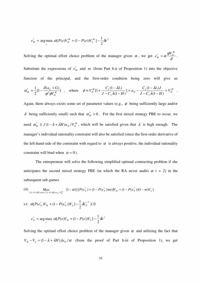
55
=*Me
e
maxarg 2
2
1]))(1()([ eVePVeP
M
L
M
H δα −−+
Solving the optimal effort choice problem of the manager given α , we get δ
ϕα
M
D
M
Ve =* .
Substitute the expressions of *Me and m (from Part b.ii of Proposition 1) into the objective
function of the principal, and the first-order condition being zero will give us
])(
1[2
12
*
M
D
L
MV
Ga
φϕ
δα
+−= , where M
D
I
I
D
I
IM
D VHCJ
JLCa
HCJ
LCV >
−−
−−=
−−
−+≡
)1(
)1(]
)1(
)1(1[
λ
λ
λ
λφ .
Again, there always exists some set of parameter values (e.g., ϕ being sufficiently large and/or
δ being sufficiently small) such that 0* >Mα . For the first mixed strategy PBE to occur, we
need M
DDM VaHf /)1(* λλα +−≥ , which will be satisfied given that λ is high enough. The
manager’s individual rationality constraint will also be satisfied (since the first-order derivative of
the left-hand-side of the constraint with regard to α is always positive, the individual rationality
constraint will bind when 0=α ).
The entrepreneur will solve the following simplified optimal contracting problem if she
anticipates the second mixed strategy PBE (in which the RA never audits at t = 2) in the
subsequent sub-games.
(4)M
DD VaHfHf
Max/)1()1( λλαλλ +−<<+−
)1))((1()]))(1()()[1( ***LNHNN VmePVmePeP −−+−+− α
s.t. 02
1]))(1()([
2*** ≥−−+ NLNHN eVePVeP δα
=*Ne
e
maxarg 2
2
1]))(1()([ eVePVeP LH δα −−+
Solving the optimal effort choice problem of the manager given α and utilizing the fact that
αλλ /)1( DLH faHVV +−=− (from the proof of Part b.iii of Proposition 1), we get

56
δ
λλϕ DN
faHe
)1(* +−= , which is independent of α . Thus, )( *
NeP is also independent of α .
Substitute the expressions of m (from Part b.iii of Proposition 1) into the objective function of the
principal, and it can be shown that the first-order derivative of the objective function with regards
to α is always negative. Thus the principal will want to minimize α in this case (this is
intuitive given that the managerial effort level is independent of α ). It can also be verified that the
left-hand-side of the individual rationality constraint of the manager can be simplified to
δ
λλϕα
2
])1([ 2D
L
faHV
+−+ , which is always greater than zero. Therefore, the entrepreneur will
pick α to be as close to )1( Hf λλ +− as possible as, but can never set )1(* HfN λλα +−=
(recall that we must have )1(* HfN λλα +−> , otherwise, the separating equilibrium will occur in
the subsequent sub-games). The optimal *Nα hence does not exist. Q.E.D.
Proof of Proposition 3: For a given set of exogenous parameters Ω , let
)),(()( * ΩΩ=Ω T
CritCrit
T αλλ , where )),(( * ΩΩT
Crit αλ is the function defined in equation (8)
evaluated at )(* Ω= Tαα , conditional on all the relevant parameters in Ω . From equation (13) it
is clear that 21)(* <ΩTα . From equation (8) we then have 0)( >ΩCrit
Tλ , thus there will always
exist sufficiently low value of λ such that )(Ω< Crit
Tλλ and the separating equilibrium occurs.
Q.E.D.
Proof of Proposition 4: There always exists some subset of Ω such that 0* >Tα (e.g., given
that the coefficient of disutility of effort, δ , is small and/or marginal productivity of effort, ϕ , is
big), thus (since fHT >*α ) we will have 1)( <ΩCrit
Tλ . Therefore, for sufficiently high value of
λ such that )(Ω> Crit
Tλλ , the separating equilibrium cannot exist, thus fraud must exist in any

57
alternative equilibrium. In that case, depending on different parameter values, either the pooling
equilibrium or mixed strategy equilibrium obtains, or no equilibrium exists. Similarly, there
always exist some subset of Ω such that 0* >Pα (e.g., δ is small and/or ϕ is big and λ is
high), thus (since fHP >*α ) we will have 1)( <ΩCrit
Pλ . Therefore, for sufficiently high value of
λ such that )(Ω> Crit
Pλλ , if )](),([)(* ΩΩ≥Ω Crit
Manager
Crit
RA PPMaxP , the pooling equilibrium
obtains. Also, there always exist some subset of Ω such that 0* >Mα (e.g., δ is small and/or
ϕ is big), thus (given that fHV
aM
D
D
M )(* >α ) we will have 11
)(1 *
<−
−
H
faV D
M
DMα . Thus, for
sufficiently high value of λ such that H
faV D
M
DM
−
−≥
1
)(1 *αλ , if
)](),([)(* ΩΩ<Ω Crit
Manager
Crit
RA PPMaxP , the fully mixed equilibrium obtains.
From Proposition 2, it is easy to verify that **MT αα > . For sufficiently high value of λ ,
we also have ***MTP ααα >> , thus,
)]),((),([)]),((),([ ** ΩΩΩ≥ΩΩΩ P
Crit
Manager
Crit
RAM
Crit
Manager
Crit
RA PPMaxPPMax αα .
It is also easy to verify that
φδ
ϕλλ
δ
ϕ
22)(
)(2])1([
2)(
2*
2* Ga
VPJa
BafaHJaP LM
DM
D
L
DDP
+−=Ω>
+
+−+−++=Ω .
Therefore, for some subset of Ω such that 1)( <ΩCrit
Pλ and 11
)(1 *
<−
−
H
faV D
M
DMα (i.e., 0* >Pα
and 0* >Mα ; recall that 0→H ), for sufficiently high value of λ such that
H
f
H
faV PD
M
DM
−
−>
−
−≥
1
1
1
)(1 ** ααλ , we should have either
i) )),((),([)]),((),([)()( **** ΩΩΩ≥ΩΩΩ>Ω>Ω P
Crit
Manager
Crit
RAM
Crit
Manager
Crit
RAMP PPMaxPPMaxPP αα ,

58
or
ii) )()()),((),([)]),((),([ **** Ω>Ω>ΩΩΩ≥ΩΩΩ MPP
Crit
Manager
Crit
RAM
Crit
Manager
Crit
RA PPPPMaxPPMax αα ,
or
iii) )()),((),([)]),((),([)( **** Ω>ΩΩΩ≥ΩΩΩ>Ω MP
Crit
Manager
Crit
RAM
Crit
Manager
Crit
RAP PPPMaxPPMaxP αα ,
or
iv) )()),((),([)()]),((),([ **** Ω>ΩΩΩ>Ω>ΩΩΩ MP
Crit
Manager
Crit
RAPM
Crit
Manager
Crit
RA PPPMaxPPPMax αα ,
or
v) )),((),([)()]),((),([)( **** ΩΩΩ>Ω>ΩΩΩ>Ω P
Crit
Manager
Crit
RAMM
Crit
Manager
Crit
RAP PPMaxPPPMaxP αα ,
or
vi) )),((),([)()()]),((),([ **** ΩΩΩ>Ω>Ω>ΩΩΩ P
Crit
Manager
Crit
RAMPM
Crit
Manager
Crit
RA PPMaxPPPPMax αα .
It is clear that pooling is the only possible equilibrium under i) and fully mixed is the only possible
equilibrium under ii). Under iii) to vi), both pooling and fully mixed are possible. Which one
obtains then depends on the entrepreneurial utility (since the entrepreneur is the Stackelberg leader
in the overall game). Thus, when λ is sufficiently high, either the pooling equilibrium or the
mixed strategy equilibrium obtains. Q.E.D.