HAL Id: hal-01299161https://hal.archives-ouvertes.fr/hal-01299161

Submitted on 7 Apr 2016

HAL is a multi-disciplinary open accessarchive for the deposit and dissemination of sci-entific research documents, whether they are pub-lished or not. The documents may come fromteaching and research institutions in France orabroad, or from public or private research centers.

L’archive ouverte pluridisciplinaire HAL, estdestinée au dépôt et à la diffusion de documentsscientifiques de niveau recherche, publiés ou non,émanant des établissements d’enseignement et derecherche français ou étrangers, des laboratoirespublics ou privés.

The stochastic topic block model for the clustering ofvertices in networks with textual edges

Charles Bouveyron, P Latouche, R Zreik

To cite this version:Charles Bouveyron, P Latouche, R Zreik. The stochastic topic block model for the clustering ofvertices in networks with textual edges. Statistics and Computing, Springer Verlag (Germany), 2016,<10.1007/s11222-016-9713-7>. <hal-01299161>

The Stochastic Topic Block Model for the Clustering ofNetworks with Textual Edges

C. Bouveyron1, P. Latouche2, R. Zreik1,2

April 7, 20161Laboratoire MAP5, UMR CNRS 8145

Université Paris Descartes & Sorbonne Paris Cité

2Laboratoire SAMM, EA 4543Université Paris 1 Panthéon-Sorbonne

Abstract

Due to the significant increase of communications between individuals via social medias (Face-book, Twitter) or electronic formats (email, web, co-authorship) in the past two decades, networkanalysis has become a unavoidable discipline. Many random graph models have been proposedto extract information from networks based on person-to-person links only, without taking intoaccount information on the contents. In this paper, we have developed the stochastic topic blockmodel (STBM) model, a probabilistic model for networks with textual edges. We address herethe problem of discovering meaningful clusters of vertices that are coherent from both the networkinteractions and the text contents. A classification variational expectation-maximization (C-VEM)algorithm is proposed to perform inference. Simulated data sets are considered in order to assessthe proposed approach and highlight its main features. Finally, we demonstrate the effectivenessof our model on two real-word data sets: a communication network and a co-authorship network.

1 IntroductionRanging from communication to co-authorship networks, it is nowadays extremely frequent to observenetworks with textual edges. It is obviously of strong interest to be able to model and cluster thosenetworks using information on both the network structure and the text contents. Techniques able toprovide such a clustering would allow a deeper understanding of the studied networks. As a motivatingexample, Figure 1 shows a network made of 3 “communities” where one of the communities can in factbe split into two separate groups based on the topics of communication between nodes of these groups.Despite the important efforts in both network analysis and text analytics, only a few works have focusedon the joint modeling and clustering of network vertices and textual edges.

Statistical models for network analysis On the on hand, the statistical analysis of networks hasonly emerged fifteen year ago with the seminal work of Hoff et al. (2002) and, since, the topic hasknown a strong development. In particular, statistical methods have imposed theirselves as efficientand flexible techniques for network clustering. Most of those methods look for specific structures,so called communities, which exhibit a transitivity property such that nodes of the same communityare more likely to be connected (Hofman and Wiggins, 2008). A popular approach for communitydiscovering, though asymptotically biased (Bickel and Chen, 2009), is based on the modularity scoregiven by Girvan and Newman (2002). Alternative methods usually rely on the latent position clustermodel (LPCM) of Handcock et al. (2007) or stochastic block model (SBM) (Wang and Wong, 1987;Nowicki and Snijders, 2001). The LPCM model assumes that the links between the vertices dependon their positions in a social latent space and allows the simultaneous visualization and clustering of anetwork. The SBM model is a flexible random graph model which can also characterize communities,but not only. It is based on a probabilistic generalization of the method applied by White et al.(1976) on Sampson’s famous monastery (Fienberg and Wasserman, 1981). It assumes that each vertexbelongs to a latent group, and that the probability of connection between a pair of vertices dependsexclusively on their group. Because no specific assumption is made on the connection probabilities,various types of structures of vertices can be taken into account. While SBM was originally developed

1

Figure 1: A sample network made of 3 “communities” where one of the communities is made of twotopic-specific groups. The left panel only shows the observed (binary) edges in the network. The centerpanel shows the network with only the partition of edges into 3 topics (edge colors indicate the topicsof texts). The right panel shows the network with the clustering of both nodes and edges (vertice colorsindicate the groups). The latter visualization allows to see the topic-conditional structure of one of thethree communities.

to analyze mainly binary networks, many extensions have been proposed since to deal for instance withvalued edges (Mariadassou et al., 2010), categorical edges (Jernite et al., 2014) or to take into accountprior information (Zanghi et al., 2010; Matias and Robin, 2014). Note that other extensions of SBMhave focused on looking for overlapping clusters (Airoldi et al., 2008; Latouche et al., 2011) or onthe modeling of dynamic networks (Matias and Miele, 2016; Yang et al., 2011; Xu and Hero III, 2013;Bouveyron et al., 2016). The inference of SBM-like models is usually done using variational expectationmaximization (VEM) (Daudin et al., 2008), variational Bayes EM (VBEM) (Latouche et al., 2012),or Gibbs sampling (Nowicki and Snijders, 2001). Moreover, we emphasize that various strategies havebeen derived to estimates the number of corresponding clusters using model selection criteria (Daudinet al., 2008; Latouche et al., 2012), allocation sampler (Mc Daid et al., 2013), greedy search (Cômeand Latouche, 2015), or non parametric schemes (Kemp et al., 2006). We refer to (Salter-Townshendet al., 2012) for a recent overview of statistical models for network analysis.

Statistical models for text analytics On the other hand, statistical model for texts has appearedat the end of the last century with an early model described by Papadimitriou et al. (1998) for latentsemantic indexing (LSI) (Deerwester et al., 1990). LSI is known in particular for allowing to recoverlinguistic notions such as synonymy and polysemy from “term frequency - inverse document frequency”(tf-idf) data. Hofmann (1999) proposed an alternative model for LSI, called probabilistic latent semanticanalysis (pLSI), which models each word within a document using a mixture model. In pLSI, eachmixture component is modeled by a multinomial random variable and the latent groups can be viewedas “topics”. Thus, each word is generated from a single topic and different words in a document can begenerated from different topics. However, it may be criticized that pLSI has no model at the documentlevel and that it may suffer from overfitting. Notice that pLSI can also be viewed has an extension ofthe mixture of unigrams, proposed by Nigam et al. (2000). The model which finally concentrates alldesired feature was proposed by Blei et al. (2003) and is called latent Dirichlet allocation (LDA). TheLDA model has rapidly become a standard tool in statistical text analytics and is even used in differentscientific fields such has image analysis (Lazebnik et al., 2006) or transportation research (Côme et al.,2014) for instance. The idea of LDA is that documents are represented as random mixtures over latenttopics, where each topic is characterized by a distribution over words. LDA is therefore similar to pLSIexcept that the topic distribution in LDA has a Dirichlet prior. Note that a limitation of LDA wouldbe the inability to take into account possible topic correlations. This is due to the use of the Dirichletdistribution to model the variability among the topic proportions. To overcome this limitation, thecorrelated topic model (CTM) has been recently developed by Blei and Lafferty (2006). Similarly, the

2

relational topic model (RTM) (Chang and Blei, 2009) models the links between documents as binaryrandom variables conditioned on their contents, but ignoring the community ties between the authors ofthese documents. Notice that the “itopic” model (Sun et al., 2009) extends RTM to weighted networks.The reader may refer to Blei (2012) for an overview on probabilistic topic models.

Statistical models for the joint analysis of texts and networks Finally, a few recent works havefocused on the joint modeling of texts and networks. Those works are mainly motivated by the will ofanalyzing social networks, such as Twitter or Facebook, or electronic communication networks. Someof them are partially based on LDA: the author-topic (AT) (Steyvers et al., 2004; Rosen-Zvi et al.,2004) and the author-recipient-topic (ART) (McCallum et al., 2005) models. The AT model extendsLDA to include authorship information whereas the ART model includes authorships and informationabout the recipients. Though potentially powerful, these models do not take into account the networkstructure (communities, stars, ...) while the concept of a community is very important in the context ofsocial networks, in the sense that a community is a group of users sharing similar interests. Among themost advanced models for the joint analysis of texts and networks, the first models which explicitly takeinto account both text contents and network structure are the community-user-topic (CUT) modelsproposed by (Zhou et al., 2006). Two models are proposed: CUT1 and CUT2, which differs on the waythey construct the communities. Indeed, CUT1 determines the communities only based on the networkstructure whereas CUT2 model the communities based on the content information solely. The CUTmodels are therefore dealing each with only a part of the problem we are interested to address here.It is also worth noticing that the authors of these models rely for inference on Gibbs sampling whichmay prohibit their use on large networks. A second attempt was made by Pathak et al. (2008) whoextended the ART model by introducing the community-author-recipient-topic (CART) model. TheCART model adds to the ART model that authors and recipients belong to latent communities andallows CART to recover groups of nodes that are homogenous both regarding the network structureand the message contents. Notice that CART allows the nodes to be part of multiple communities andeach couple of actors to have a specific topic. Thus, though extremely flexible, CART is also a highlyparametrized model. In addition, the recommended inference procedure based on Gibbs sampling mayalso prohibit its application to large networks. More recently, the topic-link LDA (Liu et al., 2009)also performs topic modeling and author community discovery in a unified framework. As its namesuggests, topic-link LDA extends LDA with a community layer where the link between two documents(and consequently its authors) depends on both topic proportions and author latent features through alogistic transformation. However, whereas CART focuses only on directed networks, topic-link LDA isonly able to deal with undirected networks. On the positive side, the authors derive a variational EMalgorithm for inference, allowing topic-link LDA to eventually be applied to large networks. Finally, afamily of 4 topic-user-community models (TUCM) were proposed by Sachan et al. (2012). The TUCMmodels are designed such that they can find topic-meaningful communities in networks with differenttypes of edges. This in particular relevant in social networks such as Twitter where different typesof interactions (followers, tweet, re-tweet, ...) exist. Another specificity of the TUCM models is thatthey allow both multiple community and topic memberships. Inference is also done here through Gibbssampling, implying a possible scale limitation.

Contributions of the present work We propose here a new generative model for the clustering ofnetworks with textual edges, such as communication or co-authorship networks. Conversely to existingworks which have either too simple or highly-parametrized models for the network structure, our modelrelies for the network modeling on the SBM model which offers a sufficient flexibility with a reasonablecomplexity. This modeling is also one of the few models able to both recover structures such ascommunities, stars or disassortative clusters. Regarding the topic modeling, our model is based on theLDA model, in which the topics will be conditioned on the latent groups. Thus, the proposed modelingwill be able to exhibit node partitions that are meaningful both regarding the network structure and thetopics, with a model of limited complexity, highly interpretable, and for both directed and undirectednetworks. In addition, the proposed inference procedure – a classification-VEM algorithm – allows theuse of our model on large-scale networks.

3

Organization of the paper The proposed model, named stochastic topic block model (STBM), isintroduced in Section 2. The model inference is discussed in Section 3 as well as model selection.Section 4 is devoted to numerical experiments highlighting the main features of the proposed approachand proving the validity of the inference procedure. Two applications to real-world networks (the Enronemail and the Nips co-authorship networks) are presented in Section 5. Section 6 finally provides someconcluding remarks.

2 The modelThis section presents the notations used in the paper and introduces the STBM model. The jointdistributions of the model to create edges and the corresponding documents are also given.

2.1 Context and notations

A directed network with M vertices, described by its M ×M adjacency matrix A, is considered. Thus,Aij = 1 if there is an edge from vertex i to vertex j, 0 otherwise. The network is assumed not to haveany self-loop and therefore Aii = 0 for all i. If an edge from i to j is present, then it is characterizedby a set of Nij documents, denoted Wij = (W d

ij)d. Each document W dij is made of a collection of Nd

ij

words W dij = (W dn

ij )n. In the directed scenario considered, Wij can model for instance a set of emailsor text messages sent from actor i to actor j. Note that all the methodology proposed in this papereasily extends to undirected networks. In such a case, Aij = Aji and W d

ij = W dji for all i and j. The

set W dij of documents can then model for example books or scientific papers written by both i and j.

In the following, we denote W = (Wij)ij the set of all documents exchanged, for all the edges presentin the network.

Our goal is to cluster the vertices into Q latent groups sharing homogeneous connection profiles, i.e.find an estimate of the set Y = (Y1, . . . , YM ) of latent variables Yi such that Yiq = 1 if vertex i belongsto cluster q, and 0 otherwise. Although in some cases, discrete or continuous edges are taken intoaccount, the literature on networks focuses on modeling the presence of edges as binary variables. Theclustering task then consists in building groups of vertices having similar trends to connect to others. Inthis paper, the connection profiles are both characterized by the presence of edges and the documentsbetween pairs of vertices. Therefore, we aim at uncovering clusters by integrating these two sourcesof information. Two nodes in the same cluster should have the same trend to connect to others, andwhen connected, the documents they are involved in should be made of words related to similar topics.

2.2 Modeling the presence of edges

In order to model the presence of edges between pairs of vertices, a stochastic block model (Wang andWong, 1987; Nowicki and Snijders, 2001) is considered. Thus, the vertices are assumed to be spreadinto Q latent clusters such that Yiq = 1 if vertex i belongs to cluster q, and 0 otherwise. In practice,the binary vector Yi is assumed to be drawn from a multinomial distribution

Yi ∼M (1, ρ = (ρ1, . . . , ρQ)) ,

where ρ denotes the vector of class proportions. By construction,∑Qq=1 ρq = 1 and

∑Qq=1 Ziq = 1,∀i.

An edge from i to j is then sampled from a Bernoulli distribution, depending on their respectiveclusters

Aij |YiqYjr = 1 ∼ B(πqr). (1)

In words, if i is in cluster q and j in r, then Aij is 1 with probability πqr. In the following, we denoteπ the Q×Q matrix of connection probabilities. Note that in the undirected case, π is symmetric.

All vectors Yi are sampled independently, and given Y = (Y1, . . . , YM ), all edges in A are assumedto be independent. This leads to the following joint distribution

p(A, Y |ρ, π) = p(A|Y, π)p(Y |ρ),

4

where

p(A|Y, π) =

M∏i6=j

p(Aij |Yi, Yj , π)

=

M∏i6=j

Q∏q,l

p(Aij |πqr)YiqYjr ,

and

p(Y |ρ) =

M∏i=1

p(Yi|ρ)

=

M∏i=1

Q∏q=1

ρYiqq .

2.3 Modeling the construction of documents

As mentioned previously, if an edge is present from vertex i to vertex j, then a set of documentsWij = (W d

ij)d, characterizing the oriented pair (i, j), is assumed to be given. Thus, in a generativeperspective, the edges in A are first sampled using previous section. Given A, the documents inW = (Wij)ij are then constructed. The generative process we consider to build documents is stronglyrelated to the latent Dirichlet allocation (LDA) model of Blei et al. (2003). The link between STBMand LDA is made clear in the following section. The STBM model relies on two concepts at the coreof the SBM and LDA models respectively. On the one hand, a generalization of the SBM model wouldassume that any kind of relationships between two vertices can be explained by their latent clustersonly. In the LDA model on the other hand, the main assumption is that words in documents are drawnfrom a mixture distribution over topics, each document d having its own vector of topic proportions θd.The STBM model combines these two concepts to introduce a new generative procedure for documentsin networks.

Each pair of clusters (q, r) of vertices is first associated to a vector of topic proportions θqr = (θqrk)ksampled independently from a Dirichlet distribution

θqr ∼ Dir (α = (α1, . . . , αK)) ,

such that∑Kk=1 θqrk = 1,∀(q, r). We denote θ = (θqr)qr. The nth word W dn

ij of documents d in Wij

is then associated to a latent topic vector Zdnij assumed to be drawn from a multinomial distribution,depending on the latent vectors Yi and Yj

Zdnij | {YiqYjrAij = 1, θ} ∼ M (1, θqr = (θqr1, . . . , θqrK)) . (2)

Note that∑Kk=1 Z

dnkij = 1,∀(i, j, d), Aij = 1. Equations (1) and (2) are related: they both involve the

construction of random variables depending on the cluster assignment of vertices i and j. Thus, if anedge is present (Aij = 1) and if i is in cluster q and j in r, then the word W dn

ij is in topic k (Zdnkij = 1)with probability θqrk.

Then, given Zdnij , the word W dnij is assumed to be drawn from a multinomial distribution

W dnij |Zdnkij = 1 ∼M (1, βk = (βk1, . . . , βkV )) , (3)

where V is the number of (different) words in the vocabulary considered and∑Vv=1 βkv = 1,∀k.

Therefore, if W dnij is from topic k, then it is associated to word v of the vocabulary (W dnv

ij = 1) withprobability βkv. Equations (2) and (3) lead to the following mixture model for words over topics

W dnij | {YiqYjrAij = 1, θ} ∼

K∑k=1

θqrkM (1, βk) ,

where the K × V matrix β = (βkv)kv of probabilities does not depend on the cluster assignments.Note that words of different documents d and d

′in Wij have the same mixture distribution which only

5

w

Zθα

β

Aij

Y ρ

Π

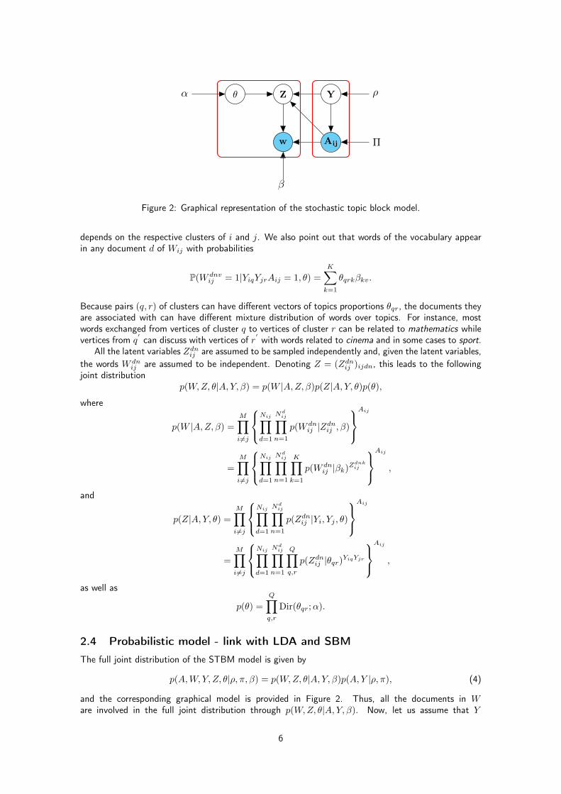
Figure 2: Graphical representation of the stochastic topic block model.

depends on the respective clusters of i and j. We also point out that words of the vocabulary appearin any document d of Wij with probabilities

P(W dnvij = 1|YiqYjrAij = 1, θ) =

K∑k=1

θqrkβkv.

Because pairs (q, r) of clusters can have different vectors of topics proportions θqr, the documents theyare associated with can have different mixture distribution of words over topics. For instance, mostwords exchanged from vertices of cluster q to vertices of cluster r can be related to mathematics whilevertices from q

′can discuss with vertices of r

′with words related to cinema and in some cases to sport.

All the latent variables Zdnij are assumed to be sampled independently and, given the latent variables,the words W dn

ij are assumed to be independent. Denoting Z = (Zdnij )ijdn, this leads to the followingjoint distribution

p(W,Z, θ|A, Y, β) = p(W |A,Z, β)p(Z|A, Y, θ)p(θ),

where

p(W |A,Z, β) =

M∏i 6=j

Nij∏d=1

Ndij∏

n=1

p(W dnij |Zdnij , β)

Aij

=

M∏i 6=j

Nij∏d=1

Ndij∏

n=1

K∏k=1

p(W dnij |βk)Z

dnkij

Aij

,

and

p(Z|A, Y, θ) =

M∏i6=j

Nij∏d=1

Ndij∏

n=1

p(Zdnij |Yi, Yj , θ)

Aij

=

M∏i6=j

Nij∏d=1

Ndij∏

n=1

Q∏q,r

p(Zdnij |θqr)YiqYjr

Aij

,

as well as

p(θ) =

Q∏q,r

Dir(θqr;α).

2.4 Probabilistic model - link with LDA and SBM

The full joint distribution of the STBM model is given by

p(A,W, Y, Z, θ|ρ, π, β) = p(W,Z, θ|A, Y, β)p(A, Y |ρ, π), (4)

and the corresponding graphical model is provided in Figure 2. Thus, all the documents in Ware involved in the full joint distribution through p(W,Z, θ|A, Y, β). Now, let us assume that Y

6

is available. It then possible to reorganize the documents in W such that W = (W̃qr)qr whereW̃qr =

{W dij ,∀(d, i, j), YiqYjrAij = 1

}is the set of all documents exchanged from any vertex i in

cluster q to any vertex j in cluster r. As mentioned in the previous section, each word W dnij has a

mixture distribution over topics which only depends on the clusters of i and j. Because all words inW̃qr are associated with the same pair (q, r) of clusters, they share the same mixture distribution.Removing temporarily the knowledge of (q, r), i.e. simply seeing W̃qr as a document d, the samplingscheme described previously then corresponds to the one of a LDA model with D = Q2 independentdocuments W̃qr, each document having its own vector θqr of topic proportions. The model is thencharacterized by the matrix β of probabilities. Note that contrary to the original LDA model (Blei et al.,2003), the Dirichlet distributions considered for the θqr depend on a fixed vector α.

As mentioned in Section 2.2, the second part of (4) involves the sampling of the clusters and theconstruction of binary variables describing the presence of edges between pairs of vertices. Interestingly,it corresponds exactly to the complete data likelihood of the SBM model, as considered in Zanghi et al.(2008) for instance. Such a likelihood term only involves the model parameters ρ and π.

3 InferenceWe aim at maximizing the complete data log likelihood

log p(A,W, Y |ρ, π, β) = log∑Z

∫θ

p(A,W, Y, Z, θ|ρ, π, β)dθ, (5)

with respect to the model parameters (ρ, π, β) and the set Y = (Y1, . . . , YM ) of cluster membershipvectors. Note that Y is not seen here as a set of latent variables over which the log likelihood shouldbe integrated out, as in standard expectation maximization (EM) (Dempster et al., 1977) or variationalEM algorithms (Hathaway, 1986). Moreover, the goal is not to provide any approximate posteriordistribution of Y given the data and model parameters. Conversely, Y is seen here as a set of (binary)vectors for which we aim at providing estimates. This choice is motivated by the key property ofthe STBM model, i.e. for a given Y , the full joint distribution factorizes into a LDA like term andSBM like term. In particular, given Y , words in W can be seen as being drawn from a LDA modelwith D = Q2 documents (see Section 2.4), for which fast optimization tools have been derived, aspointed out in the introduction. Note that the choice of optimizing a complete data log likelihoodwith respect to the set of cluster membership vectors has been considered in the literature, for simplemixture model such as Gaussian mixture models, but also for the SBM model (Zanghi et al., 2008).The corresponding algorithm, so called classification EM (CEM) (Celeux and Govaert, 1991) alternatesbetween the estimation of Y and the estimation of the model parameters.

3.1 Variational decomposition

Unfortunately, in our case, (5) is not tractable. Moreover the posterior distribution p(Z, θ|A,W, Y, ρ, π, β)does not have any analytical form. Therefore, following the work of Blei et al. (2003) on the LDA model,we propose to rely on a variational decomposition. In the case of the STBM model, it leads to

log p(A,W, Y |ρ, π, β) = L (R(·);Y, ρ, π, β) + KL (R(·) ‖ p(·|A,W, Y, ρ, π, β)),

whereL (R(·);Y, ρ, π, β) =

∑z

∫θ

R(Z, θ) logp(A,W, Y, Z, θ|ρ, π, β)

R(Z, θ)dθ, (6)

and KL denotes the Kullback-Leibler divergence between the true and approximate posterior distribu-tions of (Z, θ), given the data and model parameters

KL (R(·) ‖ p(·|A,W, Y, ρ, π, β)) = −∑z

∫θ

R(Z, θ) logp(Z, θ|A,W, Y, ρ, π, β)

R(Z, θ)dθ.

Since log p(A,W, Y |ρ, π, β) does not depend on the distribution R(Z, θ), maximizing the lower boundL with respect to R(Z, θ) induces a minimization of the KL divergence. As in Blei et al. (2003), we

7

assume that R(Z, θ) can be factorized over the latent variables in θ and Z. In our case, this translatesinto

R(Z, θ) = R(Z)R(θ) = R(θ)

M∏i 6=j

Nij∏d=1

Ndij∏

n=1

R(Zdnij ).

3.2 Model decomposition

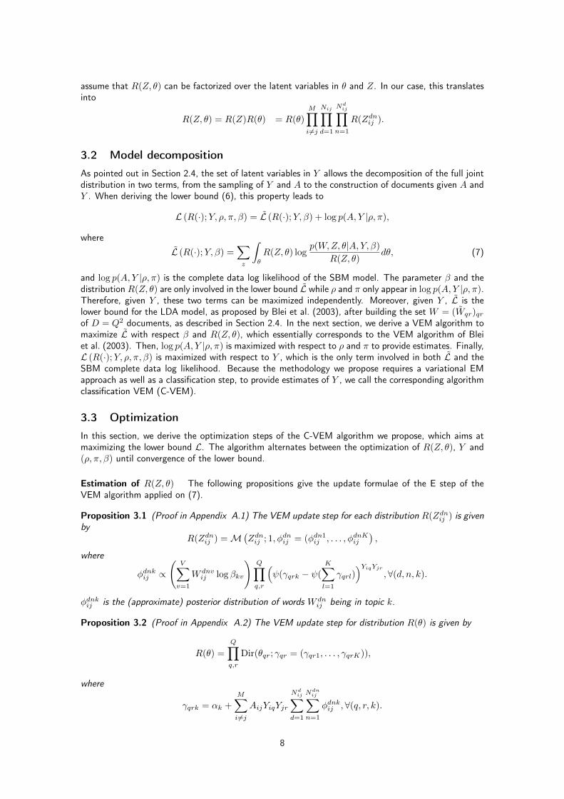
As pointed out in Section 2.4, the set of latent variables in Y allows the decomposition of the full jointdistribution in two terms, from the sampling of Y and A to the construction of documents given A andY . When deriving the lower bound (6), this property leads to

L (R(·);Y, ρ, π, β) = L̃ (R(·);Y, β) + log p(A, Y |ρ, π),

whereL̃ (R(·);Y, β) =

∑z

∫θ

R(Z, θ) logp(W,Z, θ|A, Y, β)

R(Z, θ)dθ, (7)

and log p(A, Y |ρ, π) is the complete data log likelihood of the SBM model. The parameter β and thedistribution R(Z, θ) are only involved in the lower bound L̃ while ρ and π only appear in log p(A, Y |ρ, π).Therefore, given Y , these two terms can be maximized independently. Moreover, given Y , L̃ is thelower bound for the LDA model, as proposed by Blei et al. (2003), after building the set W = (W̃qr)qrof D = Q2 documents, as described in Section 2.4. In the next section, we derive a VEM algorithm tomaximize L̃ with respect β and R(Z, θ), which essentially corresponds to the VEM algorithm of Bleiet al. (2003). Then, log p(A, Y |ρ, π) is maximized with respect to ρ and π to provide estimates. Finally,L (R(·);Y, ρ, π, β) is maximized with respect to Y , which is the only term involved in both L̃ and theSBM complete data log likelihood. Because the methodology we propose requires a variational EMapproach as well as a classification step, to provide estimates of Y , we call the corresponding algorithmclassification VEM (C-VEM).

3.3 Optimization

In this section, we derive the optimization steps of the C-VEM algorithm we propose, which aims atmaximizing the lower bound L. The algorithm alternates between the optimization of R(Z, θ), Y and(ρ, π, β) until convergence of the lower bound.

Estimation of R(Z, θ) The following propositions give the update formulae of the E step of theVEM algorithm applied on (7).

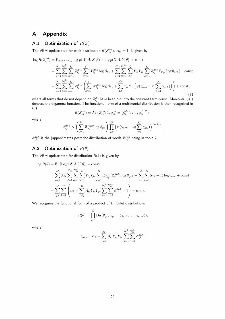
Proposition 3.1 (Proof in Appendix A.1) The VEM update step for each distribution R(Zdnij ) is givenby

R(Zdnij ) =M(Zdnij ; 1, φdnij = (φdn1ij , . . . , φdnKij

),

where

φdnkij ∝

(V∑v=1

W dnvij log βkv

)Q∏q,r

(ψ(γqrk − ψ(

K∑l=1

γqrl))YiqYjr

,∀(d, n, k).

φdnkij is the (approximate) posterior distribution of words W dnij being in topic k.

Proposition 3.2 (Proof in Appendix A.2) The VEM update step for distribution R(θ) is given by

R(θ) =

Q∏q,r

Dir(θqr; γqr = (γqr1, . . . , γqrK)),

where

γqrk = αk +

M∑i 6=j

AijYiqYjr

Ndij∑

d=1

Ndnij∑

n=1

φdnkij ,∀(q, r, k).

8

Estimation of the model parameters Maximizing the lower bound L in (7) is used to provideestimates of the model parameters (ρ, π, β). We recall that β is only involved in L̃ while (ρ, π) onlyappear in the SBM complete data log likelihood.

Proposition 3.3 The estimates of β, ρ, and π, are given by

βkv ∝M∑i6=j

Aij

Nij∑d=1

Ndnij∑

n=1

φdnkij W dnvij ,∀(k, v),

ρq ∝Q∑i=1

Yiq,∀q,

πqr =

∑Mi 6=j∑Qq,r YiqYjrAij∑M

i 6=j∑Qq,r YiqYjr

,∀(q, r).

Estimation of Y At this step, the model parameters (ρ, π, β) along with the distribution R(Z, θ)are held fixed. Therefore, the lower bound L in (7) only involves the set Y of cluster membershipvectors. Looking for the optimal solution Y maximizing this bound is not feasible since it involvestesting the QM possible cluster assignments. However, heuristics are available to provide local maximafor this combinatorial problem. These so called greedy methods have been used for instance to lookfor communities in networks by Newman (2004); Blondel et al. (2008) but also for the SBM model(Côme and Latouche, 2015). They are sometimes referred to as on line clustering methods (Zanghiet al., 2008).

The algorithm cycles randomly through the vertices. At each step, a single vertex is considered andall membership vectors Yj are held fixed, except Yi. If i is currently in cluster q, then the method looksfor every possible label swap, i.e. removing i from cluster q and assigning it to a cluster r 6= q. Thecorresponding change in the lower bound is then computed. If no label swap induces an increase in thelower bound, then Yi remain unchanged. Otherwise, the label swap that yields the maximal increaseis applied, and Yi is changed accordingly. Finally, the method terminates if a complete pass over thevertices did not lead to any increase in the lower bound.

3.4 Model selection

The C-VEM introduced in the previous section allows the estimation of R(Z, θ), Y , as well as (ρ, π, β),for a fixed number Q of clusters and a fixed number K of topics. Since a model based approach isproposed here, two STBM models will be seen as different is they have different values of Q and/orK. Therefore, the task of estimating Q and K can be viewed as a model selection problem. Manymodel selection criteria have been proposed in the literature, such as the Akaike information criterion(Akaike, 1973) (AIC) and the Bayesian information criterion (Schwarz, 1978) (BIC). In this paper, weconsider a BIC like criterion which is known to have relevant asymptotic properties (Leroux, 1992).Such a criterion estimates the marginal log likelihood using Laplace approximation.

4 Numerical experimentsThis section aims at highlighting the main features of the proposed approach on synthetic data andproving the validity of the inference algorithm presented in the previous section. Model selection isalso considered to validate the criterion choice. Numerical comparisons with state-of-the-art methodsconclude this section. Let us notice that only directed networks are considered here since they correspondto the most general case.

4.1 Simulation setup

In order to illustrate the interest of the proposed methodology, three different simulation setups will beused in this section. To simplify the characterization and facilitate the reproducibility of the experiments,we designed three different scenarios. The three simulation setups are as follows:

9

Scenario A Scenario B Scenario C

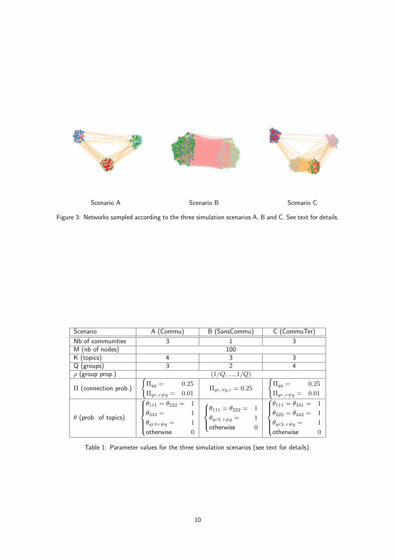
Figure 3: Networks sampled according to the three simulation scenarios A, B and C. See text for details.

Scenario A (Commu) B (SansCommu) C (CommuTer)Nb of communities 3 1 3M (nb of nodes) 100K (topics) 4 3 3Q (groups) 3 2 4ρ (group prop.) (1/Q, ..., 1/Q)

Π (connection prob.)

{Πqq = 0.25

Πqr, r 6=q = 0.01Πqr, ∀q,r = 0.25

{Πqq = 0.25

Πqr, r 6=q = 0.01

θ (prob. of topics)

θ111 = θ222 = 1

θ333 = 1

θqr4 r 6=q = 1

otherwise 0

θ111 = θ222 = 1

θqr3, r 6=q = 1

otherwise 0

θ111 = θ331 = 1

θ222 = θ442 = 1

θqr3, r 6=q = 1

otherwise 0

Table 1: Parameter values for the three simulation scenarios (see text for details).

10

• scenario A consists in networks with Q = 3 groups, corresponding to clear communities, wherepersons within a group talk preferentially about a unique topic and use a different topic whentalking with persons of other groups. Thus, those networks contain K = 4 topics.

• scenario B consists in networks with a unique community where the Q = 2 groups are onlydifferentiated by the way they discuss within and between groups. Persons within groups #1and #2 talk preferentially about topics #1 and #2 respectively. A third topic is used for thecommunications between persons of different groups.

• scenario C, finally, consists in networks with Q = 4 groups which use K = 3 topics to commu-nicate. Among the 4 groups, two groups correspond to clear communities where persons talkpreferentially about a unique topic within the communities. The two other groups correspond toa single community and are only discriminated by the topic used in the communications. Peoplefrom group #3 use topic #1 and the topic #2 is used in group #4. The third topic is used forcommunications between groups.

For all scenarios, the simulated messages are sampled from four texts from BBC news: one text is aboutthe birth of Princess Charlotte, the second one is about black holes in astrophysics, the third one isfocused on UK politics and the last one is about cancer diseases in medicine. All messages are made of150 words. Table 1 provides the parameters values for the three simulation scenarios. Figure 3 showssimulated networks according to the three simulation scenarios. It is worth noticing that all simulationscenarios have been designed such that they do not to strictly follow the STBM model and thereforethey do not favor our model in comparisons.

4.2 Introductory example

As an introductory example, we consider a network of M = 100 nodes sampled according to scenario C(3 communities, Q = 4 groups and K = 3 topics). This scenario corresponds to a situation where bothnetwork structure and topic information are needed to correctly recover the data structure. Indeed,groups #3 and #4 form a single community when looking the network structure and it is necessary tolook at the way they communicate to discriminate the two groups.

The C-VEM algorithm for STBM was run on the network with the actual number of groups andtopics (the problem of model selection will be considered in next section). Figure 4 first shows theobtained clustering, which is here perfect both regarding the simulated node and edges partitions.More interestingly, Figure 5 allows to visualize the evolution of the lower bound L along the algorithmiterations (top-left panel), the estimated model parameters Π and ρ (right panels) and the most frequentwords in the 3 found topics (left-bottom panel). It turns out that both the model parameters, Π andρ (see Table 1 for actual values), and the topic meanings are well recovered. STBM indeed perfectlyrecover the three themes that we used for simulating the textual edges: one is a “royal baby” topic,one is a political one and the last on is focused on Physics. Notice also that this result was obtainedin only a few iterations of the C-VEM algorithm, that we proposed for inferring STBM models.

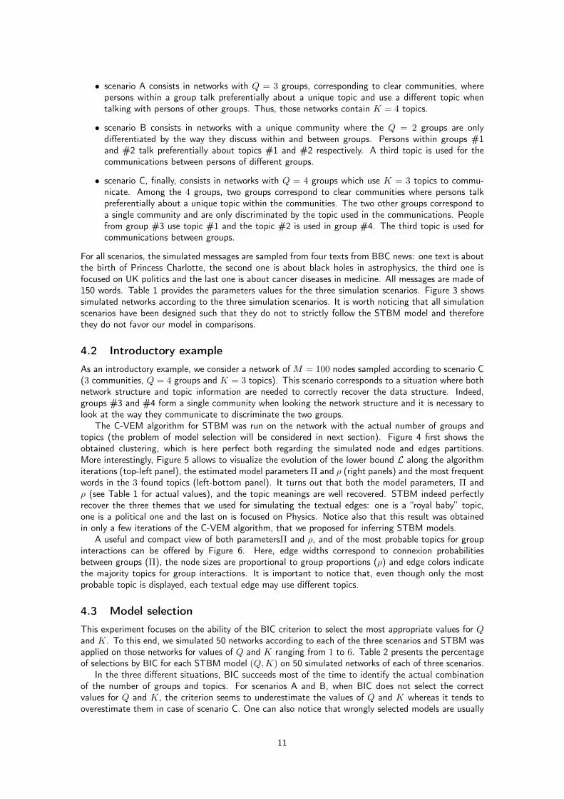
A useful and compact view of both parametersΠ and ρ, and of the most probable topics for groupinteractions can be offered by Figure 6. Here, edge widths correspond to connexion probabilitiesbetween groups (Π), the node sizes are proportional to group proportions (ρ) and edge colors indicatethe majority topics for group interactions. It is important to notice that, even though only the mostprobable topic is displayed, each textual edge may use different topics.

4.3 Model selection

This experiment focuses on the ability of the BIC criterion to select the most appropriate values for Qand K. To this end, we simulated 50 networks according to each of the three scenarios and STBM wasapplied on those networks for values of Q and K ranging from 1 to 6. Table 2 presents the percentageof selections by BIC for each STBM model (Q,K) on 50 simulated networks of each of three scenarios.

In the three different situations, BIC succeeds most of the time to identify the actual combinationof the number of groups and topics. For scenarios A and B, when BIC does not select the correctvalues for Q and K, the criterion seems to underestimate the values of Q and K whereas it tends tooverestimate them in case of scenario C. One can also notice that wrongly selected models are usually

11

Final clustering

Figure 4: Clustering result for the introductory example (scenario C). See text for details.

●

●

●

●

●

●

●

●

● ● ● ● ●

2 4 6 8 10 12

−52

0000

−50

0000

−48

0000

−46

0000

−44

0000

Lower−Bound

Iterations

Val

ue o

f the

Low

er−

Bou

nd

Connexion probabilities between groups (πq)

Recipient

Sen

der

0.23 0.01 0.01 0.23

0.01 0.26 0.01 0.01

0.01 0.01 0.23 0.01

0.25 0.02 0.01 0.26

1 2 3 4

1

2

3

4

Topics

Topic 1 Topic 2 Topic 3

event party greatgranddaughter

credit government kensington

shadow lost duke

light resentment duchess

gravity united palace

see snp queen

will kingdom cambridge

holes political charlotte

hole david birth

black seats princess

Group proportions (ρq)

Q (clusters)

Fra

ctio

n of

the

sam

ple

0.00

0.05

0.10

0.15

0.20

0.25

0.30

27

23

25 25

1 2 3 4

Figure 5: Clustering result for the introductory example (scenario C). See text for details.

12

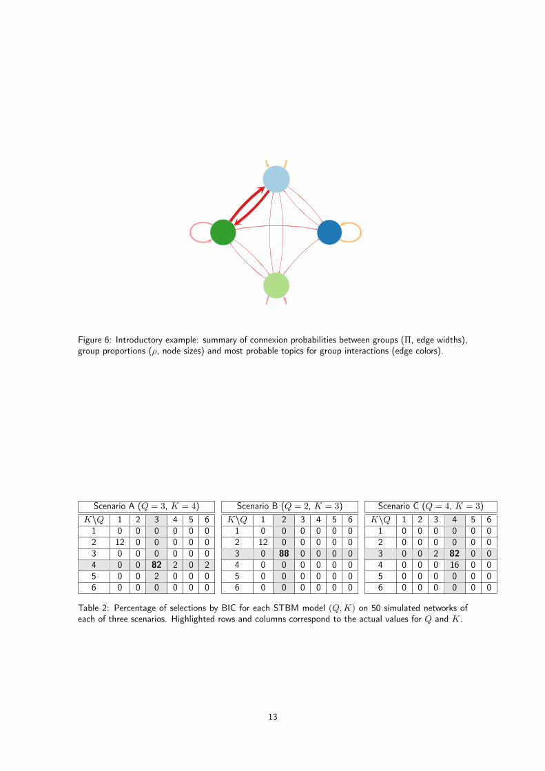
Figure 6: Introductory example: summary of connexion probabilities between groups (Π, edge widths),group proportions (ρ, node sizes) and most probable topics for group interactions (edge colors).

Scenario A (Q = 3, K = 4)K\Q 1 2 3 4 5 61 0 0 0 0 0 02 12 0 0 0 0 03 0 0 0 0 0 04 0 0 82 2 0 25 0 0 2 0 0 06 0 0 0 0 0 0

Scenario B (Q = 2, K = 3)K\Q 1 2 3 4 5 61 0 0 0 0 0 02 12 0 0 0 0 03 0 88 0 0 0 04 0 0 0 0 0 05 0 0 0 0 0 06 0 0 0 0 0 0

Scenario C (Q = 4, K = 3)K\Q 1 2 3 4 5 61 0 0 0 0 0 02 0 0 0 0 0 03 0 0 2 82 0 04 0 0 0 16 0 05 0 0 0 0 0 06 0 0 0 0 0 0

Table 2: Percentage of selections by BIC for each STBM model (Q,K) on 50 simulated networks ofeach of three scenarios. Highlighted rows and columns correspond to the actual values for Q and K.

13

Easy

Scenario A Scenario B Scenario CMethod node ARI edge ARI node ARI edge ARI node ARI edge ARISBM 1.00±0.00 – 0.01±0.01 – 0.69±0.07 –LDA – 0.97±0.06 – 1.00±0.00 – 1.00±0.00STBM 0.98±0.04 0.98±0.04 1.00±0.00 1.00±0.00 1.00±0.00 1.00±0.00

Hard1

Scenario A Scenario B Scenario CMethod node ARI edge ARI node ARI edge ARI node ARI edge ARISBM 0.01±0.01 – 0.01±0.01 – 0.01±0.01 –LDA – 0.90±0.17 – 1.00±0.00 – 0.99±0.01STBM 1.00±0.00 0.90±0.13 1.00±0.00 1.00±0.00 1.00±0.00 0.98±0.03

Hard2

Scenario A Scenario B Scenario CMethod node ARI edge ARI node ARI edge ARI node ARI edge ARISBM 1.00±0.00 – -0.01±0.01 – 0.65±0.05 –LDA – 0.21±0.13 – 0.08±0.06 – 0.09±0.05STBM 0.99±0.02 0.99±0.01 0.59±0.35 0.54±0.40 0.68±0.07 0.62±0.14

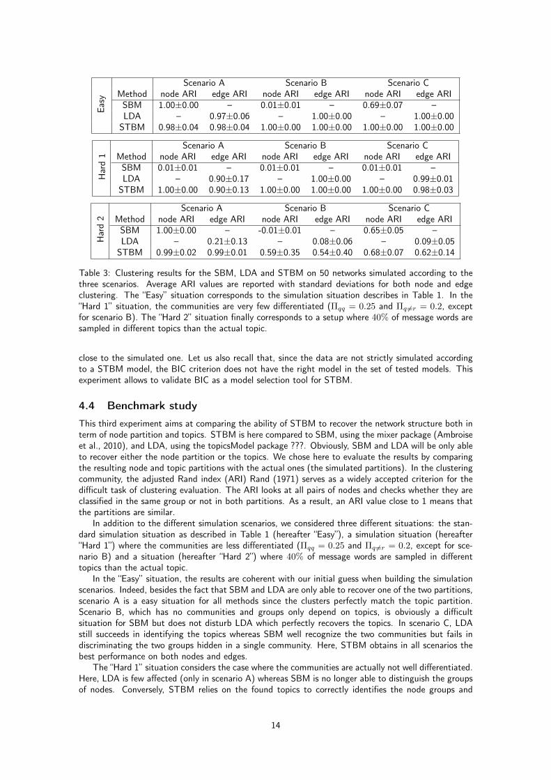
Table 3: Clustering results for the SBM, LDA and STBM on 50 networks simulated according to thethree scenarios. Average ARI values are reported with standard deviations for both node and edgeclustering. The “Easy” situation corresponds to the simulation situation describes in Table 1. In the“Hard 1” situation, the communities are very few differentiated (Πqq = 0.25 and Πq 6=r = 0.2, exceptfor scenario B). The “Hard 2” situation finally corresponds to a setup where 40% of message words aresampled in different topics than the actual topic.

close to the simulated one. Let us also recall that, since the data are not strictly simulated accordingto a STBM model, the BIC criterion does not have the right model in the set of tested models. Thisexperiment allows to validate BIC as a model selection tool for STBM.

4.4 Benchmark study

This third experiment aims at comparing the ability of STBM to recover the network structure both interm of node partition and topics. STBM is here compared to SBM, using the mixer package (Ambroiseet al., 2010), and LDA, using the topicsModel package ???. Obviously, SBM and LDA will be only ableto recover either the node partition or the topics. We chose here to evaluate the results by comparingthe resulting node and topic partitions with the actual ones (the simulated partitions). In the clusteringcommunity, the adjusted Rand index (ARI) Rand (1971) serves as a widely accepted criterion for thedifficult task of clustering evaluation. The ARI looks at all pairs of nodes and checks whether they areclassified in the same group or not in both partitions. As a result, an ARI value close to 1 means thatthe partitions are similar.

In addition to the different simulation scenarios, we considered three different situations: the stan-dard simulation situation as described in Table 1 (hereafter “Easy”), a simulation situation (hereafter“Hard 1”) where the communities are less differentiated (Πqq = 0.25 and Πq 6=r = 0.2, except for sce-nario B) and a situation (hereafter “Hard 2”) where 40% of message words are sampled in differenttopics than the actual topic.

In the “Easy” situation, the results are coherent with our initial guess when building the simulationscenarios. Indeed, besides the fact that SBM and LDA are only able to recover one of the two partitions,scenario A is a easy situation for all methods since the clusters perfectly match the topic partition.Scenario B, which has no communities and groups only depend on topics, is obviously a difficultsituation for SBM but does not disturb LDA which perfectly recovers the topics. In scenario C, LDAstill succeeds in identifying the topics whereas SBM well recognize the two communities but fails indiscriminating the two groups hidden in a single community. Here, STBM obtains in all scenarios thebest performance on both nodes and edges.

The “Hard 1” situation considers the case where the communities are actually not well differentiated.Here, LDA is few affected (only in scenario A) whereas SBM is no longer able to distinguish the groupsof nodes. Conversely, STBM relies on the found topics to correctly identifies the node groups and

14

Date

Fre

quen

cy

050

010

0015

0020

00

09/01 09/09 09/17 09/25 10/03 10/11 10/19 10/27 11/04 11/12 11/20 11/28 12/06 12/14 12/22 12/30

Figure 7: Frequency of messages between Enron employees between September 1st and December 31th,2001.

obtains, here again, excellent ARI values in the all three scenarios.The last situation, the so-called “Hard 2” case, aims to highlight the effect of the word sampling

in the recovering of the used topics. On the one hand, SBM now achieves a satisfying classificationof nodes for scenarios A and C while LDA fails in recovering the majority topic used for simulation.On those two scenarios, STBM performs well on both nodes and topics. This proves that STBM isalso able to recover the topics in a noisy situation by relying on the network structure. On the otherhand, scenario B presents an extremely difficult situation where topics are noised and there are nocommunities. Here, although both LDA and SBM fail, STBM achieves a satisfying result on bothnodes and edges. This is, once again, an illustration of the fact that the joint modeling of networkstructure and topics allows to recover complex hidden structures in a network with textual edges.

5 Application to real-world problemsIn this section, we present two applications of STBM to real-world networks: the Enron email and theNips co-authorship networks. These two data sets have been chosen because one is a directed networkof moderate size whereas the other one is undirected and of a large size.

5.1 Analysis of the Enron email network

We consider here a classical communication network, the Enron data set, which contains all emailcommunications between 149 employees of the famous company from 1999 to 2002. The original dataset is available at https://www.cs.cmu.edu/~./enron/. Here, we focus on the period September,1st to December, 31th, 2001. We chose this specific time window because it is the denser period interm of sent emails and since it corresponds to a critical period for the company. Indeed, after theannouncement early September 2001 that the company was “in the strongest and best shape that ithas ever been in”, the Securities and Exchange Commission (SEC) opened an investigation on October,31th for fraud and the company finally filed for bankruptcy on December, 2nd, 2001. By this time, itwas the largest bankruptcy in U.S. history and resulted in more than 4,000 lost jobs. Unsurprisingly,those key dates actually correspond to breaks in the email activity of the company, as shown by Figure 7.

The data set considered here contains 20 940 emails sent between the M = 149 employees. Allmessages sent between two individuals were coerced in a single meta-message. Thus, we end up with

15

Final clustering

●

●

●

●

●

●

●

●

●

●

Group 1

Group 2

Group 3

Group 4

Group 5

Group 6

Group 7

Group 8

Group 9

Group 10

Topic 1

Topic 2

Topic 3

Topic 4

Topic 5

Final clustering

●

●

●

●

●

●

●

●

●

●

Group 1

Group 2

Group 3

Group 4

Group 5

Group 6

Group 7

Group 8

Group 9

Group 10

Topic 1

Topic 2

Topic 3

Topic 4

Topic 5

Figure 8: Clustering result with STBM on the Enron data set (Sept.-Dec. 2001).

Topics

Topic 1 Topic 2 Topic 3 Topic 4 Topic 5

clock heizenrader contracts floors netting

receipt bin rto aside kilmer

gas gaskill steffes equipment juan

limits kuykendall governor numbers pkgs

elapsed ina phase assignment geaccone

injections ermis dasovich rely sara

nom allen mara assignments kay

wheeler tori california regular lindy

windows fundamental super locations donoho

forecast sheppard saturday seats shackleton

ridge named said phones socalgas

equal forces dinner notified lynn

declared taleban fantastic announcement master

interruptible park davis computer hayslett

storage ground dwr supplies deliveries

prorata phillip interviewers building transwestern

select desk state location capacity

usage viewing interview test watson

ofo afghanistan puc seat harris

cycle grigsby edison backup mmbtud

Figure 9: Most specific words for the 5 found topics with STBM on the Enron data set.

16

a data set of 1 234 directed edges between employees, each edge carrying the text of all messagesbetween two persons.

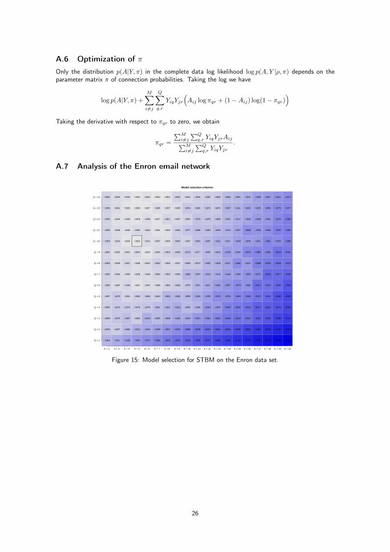
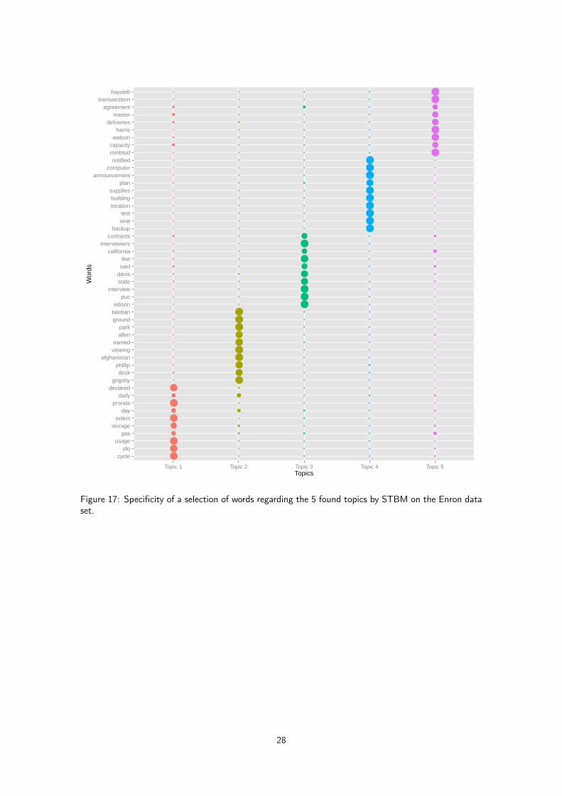
The CVEM algorithm we developed for STBM was run on these data for a number Q of groupsfrom 1 to 14 and a number K of topics from 2 to 20. As one can see on Figure 15 in Appendix A.7,the model whit the highest value was (Q,K) = (10, 5). Figure 8 shows the clustering obtained withSTBM for 10 groups of nodes and 5 topics. As previously, edge colors refer to the majority topics forthe communications between the individuals. The found topics can be easily interpreted by looking atthe most specific words of each topic, displayed in Figure 9. In a few words, we can summarize thefound topics as follows:

• Topic 1 seems to refer to the financial and trading activities of Enron,

• Topic 2 is concerned with Enron activities in Afghanistan (Enron and the Bush administrationwere suspected to work secretly with Talibans up to a few weeks before the 9/11 attacks),

• Topic 3 contains elements related to the California electricity crisis, in which Enron was involved,and which almost caused the bankruptcy of SCE-corp (Southern California Edison Corporation)early 2001,

• Topic 4 is about usual logistic issues (building equipment, computers, ...),

• Topic 5 refers to technical discussions on gas deliveries (mmBTU represents 1 million of Britishthermal unit, which is equal to 1055 joules).

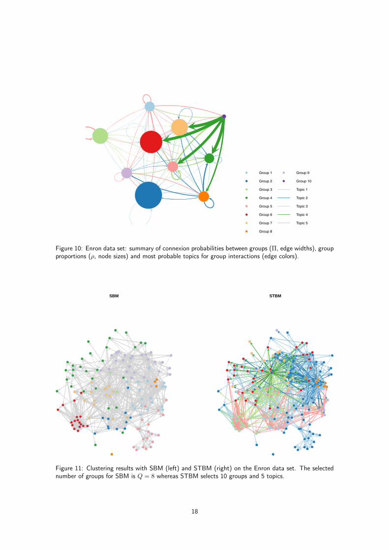
Figure 10 presents a visual summary of connexion probabilities between groups (the estimated Π matrix)and majority topics for group interactions. A few elements deserve to be highlighted in view of thissummary. First, group 10 contains a single individual who has a central place in the network and whomostly discusses about logistic issues (topic 4) with groups 4, 5, 6 and 7. Second, group 8 is made of6 individuals who mainly communicates about Enron activities in Afghanistan (topic 2) between themand with other groups. Finally, groups 4 and 6 seem to be more focused on trading activities (topic 1)whereas groups 1, 3 and 9 are dealing with technical issues on gas deliveries (topic 5).

As a comparison, the network has also been processed with SBM, using the mixer package (Ambroiseet al., 2010). The chosen numberK of groups by SBM was 8. Figure 11 allows to compare the partitionsof nodes provided by SBM and STBM. One can observe that the two partitions differ on several points.On the one hand, some communities found by SBM (the bottom-left one for instance) have been splitby STBM since some nodes use different topics than the rest of the community. On the other hand,SBM isolates two “hubs” which seem to have similar behaviors. Conversely, STBM identifies a unique“hub” and the second node is gathered with other nodes, using similar discussion topics. STBM hastherefore allowed a better and deeper understanding of the Enron network through the combination oftext contents with network structure.

5.2 Analysis of the Nips co-authorship network

This second network is a co-authorship network within a scientific conference: the Neural InformationProcessing Systems (Nips) conference. The conference was initially mainly focused on computationalneurosciences and is nowadays one of the famous conferences in statistical learning and artificial in-telligence. We here consider the data between the 1988 and 2003 editions (Nips 1–17). The dataset, available at http://robotics.stanford.edu/~gal/data.html, contains the abstracts of 2 484accepted papers from 2 740 contributing authors. The vocabulary used in the paper abstracts has14 036 words. Once the co-authorship network reconstructed, we have an undirected network between2 740 authors with 22 640 textual edges.

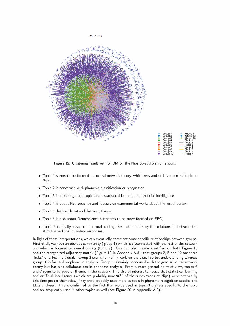
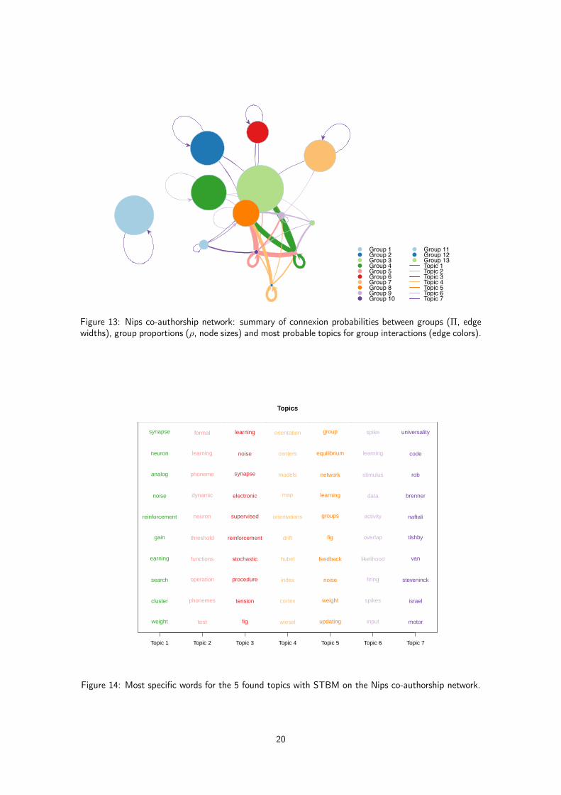
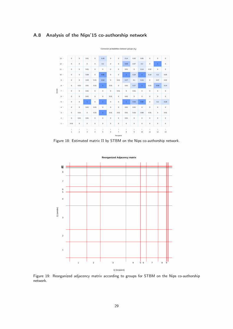
We applied STBM on this large data set and the selected model by BIC was (Q,K) = (13, 7).Figure 12 shows the clustering obtained with STBM for 13 groups of nodes and 7 topics. Due tosize and density of the network, the visualization and interpretation from this figure are actually tricky.Fortunately, the meta-view of the network shown by Figure 13 is of a greater help and allows to get aclear idea of the network organization. To this end, it is necessary to first to picture out the meaningof the found topics (see Figure 14):

17

Final clustering

●

●

●

●

●

●

●

●

●

●

Group 1

Group 2

Group 3

Group 4

Group 5

Group 6

Group 7

Group 8

Group 9

Group 10

Topic 1

Topic 2

Topic 3

Topic 4

Topic 5

Figure 10: Enron data set: summary of connexion probabilities between groups (Π, edge widths), groupproportions (ρ, node sizes) and most probable topics for group interactions (edge colors).

SBM STBM

Figure 11: Clustering results with SBM (left) and STBM (right) on the Enron data set. The selectednumber of groups for SBM is Q = 8 whereas STBM selects 10 groups and 5 topics.

18

2 4 6 8 10

24

68

10

Index

1:10

●

●

●

●

●

●

●

●

●

●

●

●

●

Group 1Group 2Group 3Group 4Group 5Group 6Group 7Group 8Group 9Group 10

Group 11Group 12Group 13Topic 1Topic 2Topic 3Topic 4Topic 5Topic 6Topic 7

Figure 12: Clustering result with STBM on the Nips co-authorship network.

• Topic 1 seems to be focused on neural network theory, which was and still is a central topic inNips,

• Topic 2 is concerned with phoneme classification or recognition,

• Topic 3 is a more general topic about statistical learning and artificial intelligence,

• Topic 4 is about Neuroscience and focuses on experimental works about the visual cortex,

• Topic 5 deals with network learning theory,

• Topic 6 is also about Neuroscience but seems to be more focused on EEG,

• Topic 7 is finally devoted to neural coding, i.e. characterizing the relationship between thestimulus and the individual responses.

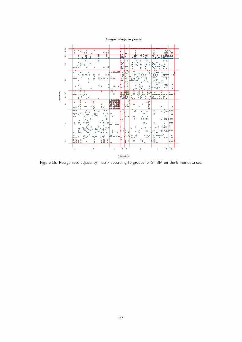
In light of these interpretations, we can eventually comment some specific relationships between groups.First of all, we have an obvious community (group 1) which is disconnected with the rest of the networkand which is focused on neural coding (topic 7). One can also clearly identifies, on both Figure 13and the reorganized adjacency matrix (Figure 19 in Appendix A.8), that groups 2, 5 and 10 are three“hubs” of a few individuals. Group 2 seems to mainly work on the visual cortex understanding whereasgroup 10 is focused on phoneme analysis. Group 5 is mainly concerned with the general neural networktheory but has also collaborations in phoneme analysis. From a more general point of view, topics 6and 7 seem to be popular themes in the network. It is also of interest to notice that statistical learningand artificial intelligence (which are probably now 90% of the submissions at Nips) were not yet bythis time proper thematics. They were probably used more as tools in phoneme recognition studies andEEG analyses. This is confirmed by the fact that words used in topic 3 are less specific to the topicand are frequently used in other topics as well (see Figure 20 in Appendix A.8).

19

5

9

12

13

5

9

12

13

5

9

12

13

5

9

12

13

5

9

12

13

5

9

12

13

5

9

12

13

5

9

12

13

5

9

12

13

5

9

12

13

5

9

12

13

5

9

12

13

5

9

12

13

5 912

13

5 912

13

5 912

13

5 912

13

5 912

13

5 912

13

5 912

13

5 912

13

5 912

13

5 912

13

5 912

13

5 912

13

5 912

13

2 4 6 8 10

24

68

10

Index

1:10

●

●

●

●

●

●

●

●

●

●

●

●

●

Group 1Group 2Group 3Group 4Group 5Group 6Group 7Group 8Group 9Group 10

Group 11Group 12Group 13Topic 1Topic 2Topic 3Topic 4Topic 5Topic 6Topic 7

Figure 13: Nips co-authorship network: summary of connexion probabilities between groups (Π, edgewidths), group proportions (ρ, node sizes) and most probable topics for group interactions (edge colors).

Topics

Topic 1 Topic 2 Topic 3 Topic 4 Topic 5 Topic 6 Topic 7

weight test fig wiesel updating input motor

cluster phonemes tension cortex weight spikes israel

search operation procedure index noise firing steveninck

earning functions stochastic hubel feedback likelihood van

gain threshold reinforcement drift fig overlap tishby

reinforcement neuron supervised orientations groups activity naftali

noise dynamic electronic map learning data brenner

analog phoneme synapse models network stimulus rob

neuron learning noise centers equilibrium learning code

synapse formal learning orientation group spike universality

Figure 14: Most specific words for the 5 found topics with STBM on the Nips co-authorship network.

20

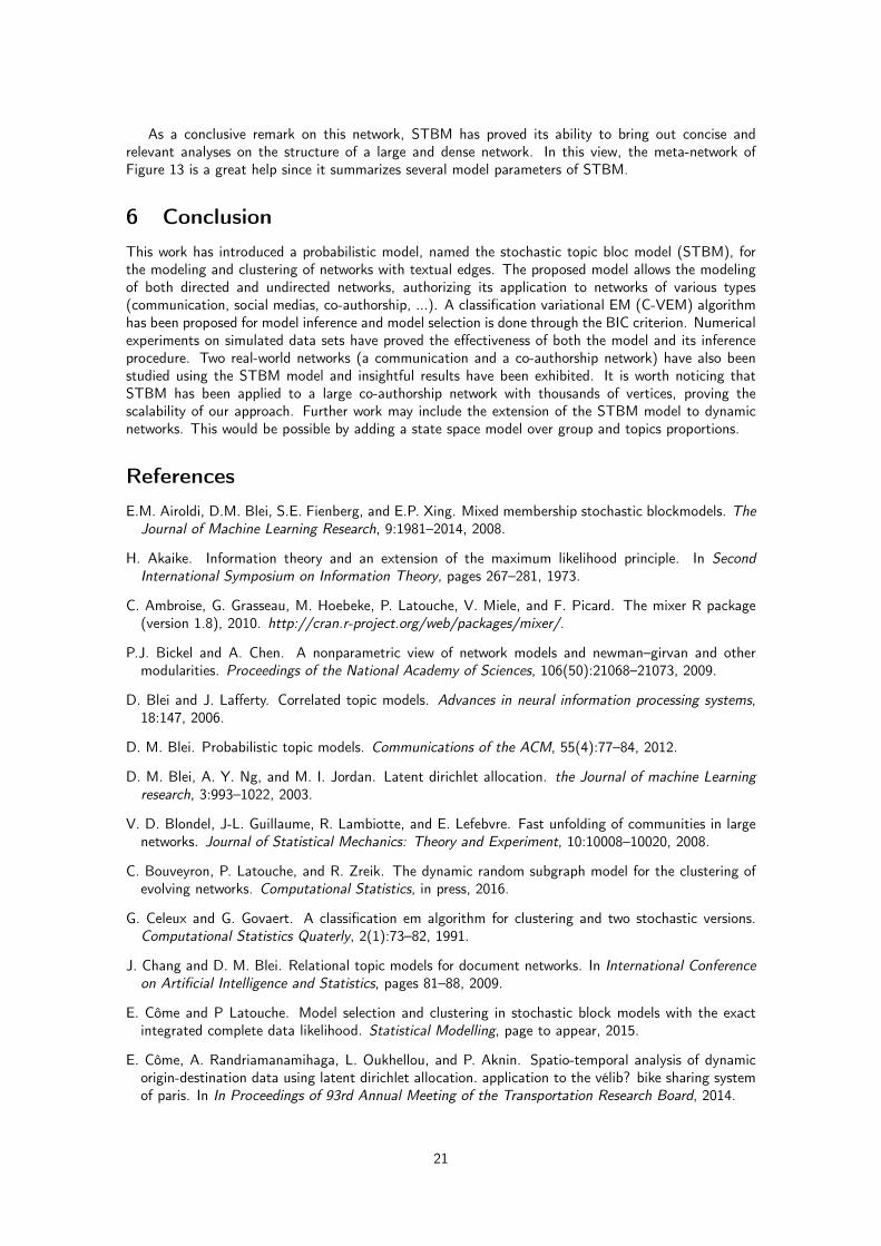
As a conclusive remark on this network, STBM has proved its ability to bring out concise andrelevant analyses on the structure of a large and dense network. In this view, the meta-network ofFigure 13 is a great help since it summarizes several model parameters of STBM.

6 ConclusionThis work has introduced a probabilistic model, named the stochastic topic bloc model (STBM), forthe modeling and clustering of networks with textual edges. The proposed model allows the modelingof both directed and undirected networks, authorizing its application to networks of various types(communication, social medias, co-authorship, ...). A classification variational EM (C-VEM) algorithmhas been proposed for model inference and model selection is done through the BIC criterion. Numericalexperiments on simulated data sets have proved the effectiveness of both the model and its inferenceprocedure. Two real-world networks (a communication and a co-authorship network) have also beenstudied using the STBM model and insightful results have been exhibited. It is worth noticing thatSTBM has been applied to a large co-authorship network with thousands of vertices, proving thescalability of our approach. Further work may include the extension of the STBM model to dynamicnetworks. This would be possible by adding a state space model over group and topics proportions.

ReferencesE.M. Airoldi, D.M. Blei, S.E. Fienberg, and E.P. Xing. Mixed membership stochastic blockmodels. TheJournal of Machine Learning Research, 9:1981–2014, 2008.

H. Akaike. Information theory and an extension of the maximum likelihood principle. In SecondInternational Symposium on Information Theory, pages 267–281, 1973.

C. Ambroise, G. Grasseau, M. Hoebeke, P. Latouche, V. Miele, and F. Picard. The mixer R package(version 1.8), 2010. http://cran.r-project.org/web/packages/mixer/.

P.J. Bickel and A. Chen. A nonparametric view of network models and newman–girvan and othermodularities. Proceedings of the National Academy of Sciences, 106(50):21068–21073, 2009.

D. Blei and J. Lafferty. Correlated topic models. Advances in neural information processing systems,18:147, 2006.

D. M. Blei. Probabilistic topic models. Communications of the ACM, 55(4):77–84, 2012.

D. M. Blei, A. Y. Ng, and M. I. Jordan. Latent dirichlet allocation. the Journal of machine Learningresearch, 3:993–1022, 2003.

V. D. Blondel, J-L. Guillaume, R. Lambiotte, and E. Lefebvre. Fast unfolding of communities in largenetworks. Journal of Statistical Mechanics: Theory and Experiment, 10:10008–10020, 2008.

C. Bouveyron, P. Latouche, and R. Zreik. The dynamic random subgraph model for the clustering ofevolving networks. Computational Statistics, in press, 2016.

G. Celeux and G. Govaert. A classification em algorithm for clustering and two stochastic versions.Computational Statistics Quaterly, 2(1):73–82, 1991.

J. Chang and D. M. Blei. Relational topic models for document networks. In International Conferenceon Artificial Intelligence and Statistics, pages 81–88, 2009.

E. Côme and P Latouche. Model selection and clustering in stochastic block models with the exactintegrated complete data likelihood. Statistical Modelling, page to appear, 2015.

E. Côme, A. Randriamanamihaga, L. Oukhellou, and P. Aknin. Spatio-temporal analysis of dynamicorigin-destination data using latent dirichlet allocation. application to the vélib? bike sharing systemof paris. In In Proceedings of 93rd Annual Meeting of the Transportation Research Board, 2014.

21

J-J. Daudin, F. Picard, and S. Robin. A mixture model for random graphs. Statistics and Computing,18(2):173–183, 2008.

S. Deerwester, S. Dumais, G. Furnas, T. Landauer, and R. Harshman. Indexing by latent semanticanalysis. Journal of the American society for information science, 41(6):391, 1990.

A. Dempster, N. Laird, and D. Rubin. Maximum likelihood from incomplete data via the EM algorithm.Journal of the Royal Statistical Society. Series B (Methodological), pages 1–38, 1977.

S.E. Fienberg and S.S. Wasserman. Categorical data analysis of single sociometric relations. SociologicalMethodology, 12:156–192, 1981.

M. Girvan and M.E.J. Newman. Community structure in social and biological networks. Proceedingsof the National Academy of Sciences, 99(12):7821, 2002.

M.S. Handcock, A.E. Raftery, and J.M. Tantrum. Model-based clustering for social networks. Journalof the Royal Statistical Society: Series A (Statistics in Society), 170(2):301–354, 2007.

R. Hathaway. Another interpretation of the EM algorithm for mixture distributions. Statistics &Probability Letters, 4(2):53–56, 1986.

P.D. Hoff, A.E. Raftery, and M.S. Handcock. Latent space approaches to social network analysis.Journal of the American Statistical Association, 97(460):1090–1098, 2002.

J.M. Hofman and C.H. Wiggins. Bayesian approach to network modularity. Physical review letters, 100(25):258701, 2008.

T. Hofmann. Probabilistic latent semantic indexing. In Proceedings of the 22nd annual internationalACM SIGIR conference on Research and development in information retrieval, pages 50–57. ACM,1999.

Y. Jernite, P. Latouche, C. Bouveyron, P. Rivera, L. Jegou, and S. Lamassé. The random subgraphmodel for the analysis of an acclesiastical network in merovingian gaul. Annals of Applied Statistics,8(1):55–74, 2014.

C. Kemp, J.B. Tenenbaum, T.L. Griffiths, T. Yamada, and N. Ueda. Learning systems of conceptswith an infinite relational model. In Proceedings of the National Conference on Artificial Intelligence,volume 21, pages 381–391, 2006.

P. Latouche, E Birmelé, and C. Ambroise. Overlapping stochastic block models with application to thefrench political blogosphere. Annals of Applied Statistics, 5(1):309–336, 2011.

P. Latouche, E Birmelé, and C. Ambroise. Variational bayesian inference and complexity control forstochastic block models. Statistical Modelling, 12(1):93–115, 2012.

S. Lazebnik, C. Schmid, and J. Ponce. Beyond bags of features: Spatial pyramid matching for recog-nizing natural scene categories. In Computer Vision and Pattern Recognition, 2006 IEEE ComputerSociety Conference on, volume 2, pages 2169–2178. IEEE, 2006.

B.G. Leroux. Consistent estimation of amixing distribution. Annals of Statistics, 20:1350–1360, 1992.

Y. Liu, A. Niculescu-Mizil, and W. Gryc. Topic-link lda: joint models of topic and author community. Inproceedings of the 26th annual international conference on machine learning, pages 665–672. ACM,2009.

M. Mariadassou, S. Robin, and C. Vacher. Uncovering latent structure in valued graphs: a variationalapproach. Annals of Applied Statistics, 4(2):715–742, 2010.

C. Matias and V. Miele. Statistical clustering of temporal networks through a dynamic stochastic blockmodel. Preprint HAL n.01167837, 2016.

C. Matias and S. Robin. Modeling heterogeneity in random graphs through latent space models: aselective review. Esaim Proc. and Surveys, 47:55–74, 2014.

22

A. Mc Daid, T.B. Murphy, Frieln N., and N.J. Hurley. Improved bayesian inference for the stochasticblock model with application to large networks. Computational Statistics and Data Analysis, 60:12–31, 2013.

A. McCallum, A. Corrada-Emmanuel, and X. Wang. The author-recipient-topic model for topic androle discovery in social networks, with application to enron and academic email. In Workshop on LinkAnalysis, Counterterrorism and Security, pages 33–44, 2005.

M. E. J. Newman. Fast algorithm for detecting community structure in networks. Physical ReviewLetter E, 69:0066133, 2004.

K. Nigam, A. McCallum, S. Thrun, and T. Mitchell. Text classification from labeled and unlabeleddocuments using em. Machine learning, 39(2-3):103–134, 2000.

K. Nowicki and T.A.B. Snijders. Estimation and prediction for stochastic blockstructures. Journal ofthe American Statistical Association, 96(455):1077–1087, 2001.

C. Papadimitriou, P. Raghavan, H. Tamaki, and S. Vempala. Latent semantic indexing: A probabilisticanalysis. In Proceedings of the tenth ACM PODS, pages 159–168. ACM, 1998.

N. Pathak, C. DeLong, A. Banerjee, and K. Erickson. Social topic models for community extraction.In The 2nd SNA-KDD workshop, volume 8. Citeseer, 2008.

W.M. Rand. Objective criteria for the evaluation of clustering methods. Journal of the AmericanStatistical association, pages 846–850, 1971.

M. Rosen-Zvi, T. Griffiths, M. Steyvers, and P. Smyth. The author-topic model for authors anddocuments. In Proceedings of the 20th conference on Uncertainty in artificial intelligence, pages487–494. AUAI Press, 2004.

M. Sachan, D. Contractor, T. Faruquie, and L. Subramaniam. Using content and interactions fordiscovering communities in social networks. In Proceedings of the 21st international conference onWorld Wide Web, pages 331–340. ACM, 2012.

M. Salter-Townshend, A. White, I. Gollini, and T. B. Murphy. Review of statistical network analysis:models, algorithms, and software. Statistical Analysis and Data Mining, 5(4):243–264, 2012.

G Schwarz. Estimating the dimension of a model. Annals of Statistics, 6:461–464, 1978.

M. Steyvers, P. Smyth, M. Rosen-Zvi, and T. Griffiths. Probabilistic author-topic models for informationdiscovery. In Proceedings of the tenth ACM SIGKDD international conference on Knowledge discoveryand data mining, pages 306–315. ACM, 2004.

Y. Sun, J. Han, J. Gao, and Y. Yu. itopicmodel: Information network-integrated topic modeling. InData Mining, 2009. ICDM’09. Ninth IEEE International Conference on, pages 493–502. IEEE, 2009.

Y.J. Wang and G.Y. Wong. Stochastic blockmodels for directed graphs. Journal of the AmericanStatistical Association, 82:8–19, 1987.

H.C. White, S.A. Boorman, and R.L. Breiger. Social structure from multiple networks. i. blockmodelsof roles and positions. American Journal of Sociology, pages 730–780, 1976.

K. Xu and A. Hero III. Dynamic stochastic blockmodels: Statistical models for time-evolving networks.In Social Computing, Behavioral-Cultural Modeling and Prediction, pages 201–210. Springer, 2013.

T. Yang, Y. Chi, S. Zhu, Y. Gong, and R. Jin. Detecting communities and their evolutions in dynamicsocial networks: a bayesian approach. Machine learning, 82(2):157–189, 2011.

H. Zanghi, C. Ambroise, and V. Miele. Fast online graph clustering via erdos-renyi mixture. Patternrecognition, 41:3592–3599, 2008.

H. Zanghi, S. Volant, and C. Ambroise. Clustering based on random graph model embedding vertexfeatures. Pattern Recognition Letters, 31(9):830–836, 2010.

D. Zhou, E. Manavoglu, J. Li, C. Giles, and H. Zha. Probabilistic models for discovering e-communities.In Proceedings of the 15th international conference on World Wide Web, pages 173–182. ACM, 2006.

23

A Appendix

A.1 Optimization of R(Z)

The VEM update step for each distribution R(Zdnij ), Aij = 1, is given by

logR(Zdnij ) = EZ\i,j,d,n,θ[log p(W |A,Z, β) + log p(Z|A, Y, θ)] + const

=

Nij∑d=1

Ndnij∑

n=1

K∑k=1

Zdnkij

V∑v=1

W dnvij log βkv +

Nij∑d=1

Ndnij∑

n=1

Q∑q,r

YiqYjr

K∑k=1

Zdnkij Eθqr [log θqrk] + const

=

Nij∑d=1

Ndnij∑

n=1

K∑k=1

Zdnkij

(V∑v=1

W dnvij log βkv +

Q∑q,r

YiqYjr

(ψ(γqrk − ψ(

K∑k=1

γqrk)))

+ const,

(8)where all terms that do not depend on Zdnij have been put into the constant term const. Moreover, ψ(·)denotes the digamma function. The functional form of a multinomial distribution is then recognized in(8)

R(Zdnij ) =M(Zdnij ; 1, φdnij = (φdn1ij , . . . , φdnKij

),

where

φdnkij ∝

(V∑v=1

W dnvij log βkv

)Q∏q,r

(ψ(γqrk − ψ(

K∑l=1

γqrl))YiqYjr

.

φdnkij is the (approximate) posterior distribution of words W dnij being in topic k.

A.2 Optimization of R(θ)

The VEM update step for distribution R(θ) is given by

logR(θ) = EZ [log p(Z|A, Y, θ)] + const

=

M∑i 6=j

Aij

Nij∑d=1

Ndij∑

n=1

Q∑q,r

YiqYjr

K∑k=1

EZdnij

[Zdnkij ] log θqrk +

Q∑q,r

K∑k=1

(αk − 1) log θqrk + const

=

Q∑q,r

K∑k=1

αk +

M∑i 6=j

AijYiqYjr

Ndij∑

d=1

Ndnij∑

n=1

φdnkij − 1

+ const.

We recognize the functional form of a product of Dirichlet distributions

R(θ) =

Q∏q,r

Dir(θqr; γqr = (γqr1, . . . , γqrK)),

where

γqrk = αk +

M∑i6=j

AijYiqYjr

Ndij∑

d=1

Ndnij∑

n=1

φdnkij .

24

A.3 Derivation of the lower bound L̃ (R(·);Y, β)The lower bound L̃ (R(·);Y, β) in (7) is given by

L̃ (R(·);Y, β) =∑z

∫θ

R(Z, θ) logp(W,Z, θ|A, Y, β)

R(Z, θ)dθ

= EspZ [log p(W |A,Z, β)] + Eθ[log p(Z|A, Y, θ)] + Eθ[log p(θ)]− EZ [logR(Z)]− Eθ[logR(θ)]

=

M∑i 6=j

Aij

Nij∑d=1

Ndnij∑

n=1

K∑k=1

φdnkij

V∑v=1

W dnvij log βkv

+

M∑i6=j

Aij

Nij∑d=1

Ndnij∑

n=1

Q∑q,r

YiqYjr

K∑k=1

φdnkij

(ψ(γqrk)− ψ(

K∑l=1

γqrl))

+

Q∑q,r

(log Γ(

K∑l=1

αk)−K∑l=1

log Γ(αl) +

K∑k=1

(αk − 1)(ψ(γqrk)− ψ(

K∑l=1

γqrl)))

−M∑i 6=j

Aij

Nij∑d=1

Ndnij∑

n=1

K∑k=1

φdnkij log φdnkij

−Q∑q,r

(log Γ(

K∑l=1

γqrl)−K∑l=1

log Γ(γqrl) +

K∑k=1

(γqrk − 1)(ψ(γqrk)− ψ(

K∑l=1

γqrl)))(9)

A.4 Optimization of β

In order to maximize the lower bound L̃ (R(·);Y, β), we isolate the terms in (9) that depend on β andadd Lagrange multipliers to satisfy the constraints

∑Vv=1 βkv = 1,∀k

L̃β =

M∑i 6=j

Aij

Nij∑d=1

Ndnij∑

n=1

K∑k=1

φdnkij

V∑v=1

W dnvij log βkv +

K∑k=1

λk(

V∑v=1

βkv − 1).

Setting the derivative, with respect to βkv, to zero, we find

βkv ∝M∑i 6=j

Aij

Nij∑d=1

Ndnij∑

n=1

φdnkij W dnvij .

A.5 Optimization of ρ

Only the distribution p(Y |ρ) in the complete data log likelihood log p(A, Y |ρ, π) depends on the pa-rameter vector ρ of cluster proportions. Taking the log and adding a Lagrange multiplier to satisfy theconstraint

∑Qq=1 ρq = 1, we have

log p(Y |ρ) +

M∑i=1

Q∑q=1

Yiq log ρq.

Taking the derivative with respect ρ to zero, we find

ρq ∝Q∑i=1

Yiq.

25

A.6 Optimization of π

Only the distribution p(A|Y, π) in the complete data log likelihood log p(A, Y |ρ, π) depends on theparameter matrix π of connection probabilities. Taking the log we have

log p(A|Y, π) +

M∑i 6=j

Q∑q,r

YiqYjr

(Aij log πqr + (1−Aij) log(1− πqr)

)Taking the derivative with respect to πqr to zero, we obtain

πqr =

∑Mi 6=j∑Qq,r YiqYjrAij∑M

i6=j∑Qq,r YiqYjr

.

A.7 Analysis of the Enron email network

Model selection criterion

K = 2 K = 3 K = 4 K = 5 K = 6 K = 7 K = 8 K = 9 K = 10 K = 11 K = 12 K = 13 K = 14 K = 15 K = 16 K = 17 K = 18 K = 19 K = 20

Q = 1

Q = 2

Q = 3

Q = 4

Q = 5

Q = 6

Q = 7

Q = 8

Q = 9

Q = 10

Q = 11

Q = 12

Q = 13

Q = 14

−1904 −1921 −1938 −1955 −1971 −1988 −2005 −2022 −2038 −2055 −2072 −2089 −2106 −2122 −2139 −2156 −2173 −2189 −2206

−1876 −1867 −1889 −1912 −1924 −1939 −1957 −1975 −1989 −2009 −2023 −2041 −2054 −2075 −2092 −2106 −2122 −2139 −2157

−1868 −1876 −1887 −1865 −1915 −1895 −1909 −1926 −1924 −1951 −1964 −1983 −2006 −2014 −2013 −2044 −2062 −2089 −2104

−1860 −1870 −1870 −1870 −1878 −1891 −1902 −1919 −1895 −1906 −1954 −1954 −1992 −2003 −2018 −2047 −2051 −2064 −2084

−1857 −1870 −1851 −1860 −1866 −1864 −1902 −1898 −1899 −1919 −1939 −1970 −1970 −1984 −1996 −2013 −2031 −2068 −2085

−1855 −1842 −1849 −1831 −1842 −1845 −1854 −1864 −1875 −1901 −1921 −1943 −1957 −1974 −1960 −2021 −2015 −2034 −2064

−1853 −1846 −1840 −1838 −1840 −1854 −1853 −1858 −1899 −1897 −1916 −1918 −1944 −1945 −1958 −1972 −2030 −2027 −2038

−1858 −1839 −1847 −1836 −1842 −1862 −1845 −1847 −1869 −1873 −1902 −1909 −1927 −1966 −1947 −1988 −2003 −2009 −2013

−1852 −1835 −1841 −1843 −1825 −1845 −1854 −1863 −1879 −1877 −1894 −1903 −1940 −1936 −1976 −1986 −1982 −2014 −2004

−1858 −1840 −1826 −1822 −1841 −1837 −1835 −1864 −1857 −1883 −1897 −1912 −1917 −1938 −1945 −1951 −1981 −1975 −1995

−1856 −1838 −1836 −1845 −1844 −1831 −1834 −1863 −1877 −1886 −1884 −1900 −1910 −1927 −1968 −1958 −1969 −1991 −1995

−1853 −1834 −1834 −1828 −1838 −1827 −1851 −1847 −1854 −1879 −1878 −1880 −1901 −1912 −1930 −1948 −1955 −1978 −1998

−1856 −1841 −1829 −1826 −1827 −1840 −1837 −1839 −1874 −1863 −1874 −1873 −1907 −1911 −1931 −1935 −1956 −1973 −1977

−1853 −1840 −1835 −1824 −1834 −1823 −1824 −1855 −1845 −1859 −1865 −1868 −1893 −1901 −1915 −1938 −1947 −1955 −1973

Figure 15: Model selection for STBM on the Enron data set.

26

Reorganized Adjacency matrix

Q (recipient)

Q (

send

er)

1 2 3 4 5 6 7 8 9

1

2

3

4

5

6

7

8

910

Figure 16: Reorganized adjacency matrix according to groups for STBM on the Enron data set.

27

●●●●●●●●●

●●

●

●

●

●

●

●

●

●

●

●

●

●

●

●

●

●

●

●

●

●

●

●

●

●

●

●

●

●

●

●

●

●

●

●

●

●

●

●

●

●

●

●

●

●

●

●

●

●

●●●●●●●●●●

●

●

●

●

●

●

●

●

●

●

●

●

●

●

●

●

●

●

●

●

●

●

●

●

●

●

●

●

●

●

●

●

●

●

●

●

●

●

●

●

●

●

●

●

●

●

●

●

●

●●●●●●●●●●

●

●

●

●

●

●

●

●

●

●

●

●

●

●

●

●

●

●

●

●

●

●

●

●

●

●

●

●

●

●

●

●

●

●

●

●

●

●

●

●

●

●

●

●

●

●

●

●

●

●●●●●●●●●●

●

●

●

●

●

●

●

●

●

●

●

●

●

●

●

●

●

●

●

●

●

●

●

●

●

●

●

●

●

●

●

●

●

●

●

●

●

●

●

●

●

●

●

●

●

●

●

●

●

●●●●●●●●●

cycleofo

usagegas

storageselect

dayprorata

dailydeclared

grigsbydesk

phillipafghanistan

viewingnamed

allenpark

groundtalebanedison

pucinterview

statedavissaiddwr

californiainterviewers

contractsbackup

seattest

locationbuildingsupplies

planannouncement

computernotified

mmbtudcapacitywatson

harrisdeliveries

masteragreement

transwesternhayslett

Topic 1 Topic 2 Topic 3 Topic 4 Topic 5Topics

Wor

ds

Figure 17: Specificity of a selection of words regarding the 5 found topics by STBM on the Enron dataset.

28

A.8 Analysis of the Nips’15 co-authorship network

Connexion probabilities between groups (πq)

Recipient

Sen

der

0.01 0 0 0 0 0 0 0 0 0 0 0 0

0 0.01 0.01 0 0 0 0 0.01 0 0 0 0 0

0 0.01 0 0.01 1 0.01 0.01 0.01 0.03 0.08 0.01 0 0.01

0 0 0.01 0.01 0 0 0 0.01 0.01 0 0 0 0

0 0 1 0 1 0 0 1 0.53 0.92 0 0.2 0.28

0 0 0.01 0 0 0.01 0 0.01 0 0 0 0 0

0 0 0.01 0 0 0 0.01 0 0.01 0 0 0 0

0 0.01 0.01 0.01 1 0.01 0 0.01 0.27 1 0.01 0.59 0.14

0 0 0.03 0.01 0.53 0 0.01 0.27 0.1 0.24 0 0.07 0.02

0 0 0.08 0 0.92 0 0 1 0.24 1 0.14 0.2 0.05

0 0 0.01 0 0 0 0 0.01 0 0.14 0.02 0 0

0 0 0 0 0.2 0 0 0.59 0.07 0.2 0 1 0

0 0 0.01 0 0.28 0 0 0.14 0.02 0.05 0 0 0

1 2 3 4 5 6 7 8 9 10 11 12 13

1

2

3

4

5

6

7

8

9

10

11

12

13

Figure 18: Estimated matrix Π by STBM on the Nips co-authorship network.

Reorganized Adjacency matrix

Q (recipient)

Q (

send

er)

1 2 3 4 5 6 7 8 9

1

2

3

4

56

7

8

910111213

Figure 19: Reorganized adjacency matrix according to groups for STBM on the Nips co-authorshipnetwork.

29

●●●●

●●●●●●

●

●

●

●

●

●

●

●

●

●

●

●

●

●

●

●

●

●

●

●

●

●

●

●

●

●

●

●

●

●

●

●

●

●

●

●

●

●

●

●

●

●

●

●

●

●

●

●

●

●

●

●

●

●

●

●

●

●

●

●

●●

●●●●●●●

●

●

●

●

●

●

●

●

●

●

●

●

●

●

●

●

●

●

●

●

●

●

●

●

●

●

●

●

●

●

●

●

●

●

●

●

●

●

●

●

●

●

●

●

●●●

●

●

●

●

●

●

●

●

●

●

●

●

●●●●●●●

●

●

●

●

●

●

●

●

●

●

●

●

●

●

●

●

●

●

●

●

●

●

●

●

●

●

●

●

●

●

●

●

●

●

●

●

●

●

●

●

●

●

●

●

●

●

●

●

●

●

●

●

●

●

●

●

●

●

●

●

●●●●●●●●●●

●

●

●

●

●

●

●

●

●

●

●

●

●

●

●

●

●

●

●

●

●

●

●

●

●

●

●

●

●

●

●

●

●

●

●

●

●

●

●

●

●

●

●

●

●

●

●

●

●

●

●

●

●

●

●

●

●

●

●

●

●●●●●●

●

●

●

●

●

●

●

●

●

●

●

●

●

●

●

●

●

●

●

●

●

●

●

●

●

●

●

●

●

●

●

●

●

●

●

●

●

●

●

●

●

●

●

●

●

●

●

●

●

●

●

●

●

●

●

●

●

●

●

●

●●●●●●●●●

●

●

●

●

●

●

●

●

●

●

●

●

●

●

●

●

●

●

●

●

●

●

●

●

●

●

●

●

●

●

●

●

●

●

●

●

●

●

●

●

●

●

●

●

●

●

●

●

●

●

●

●

●

●

●

●

●

●

●

●

●●●●●●●●●●

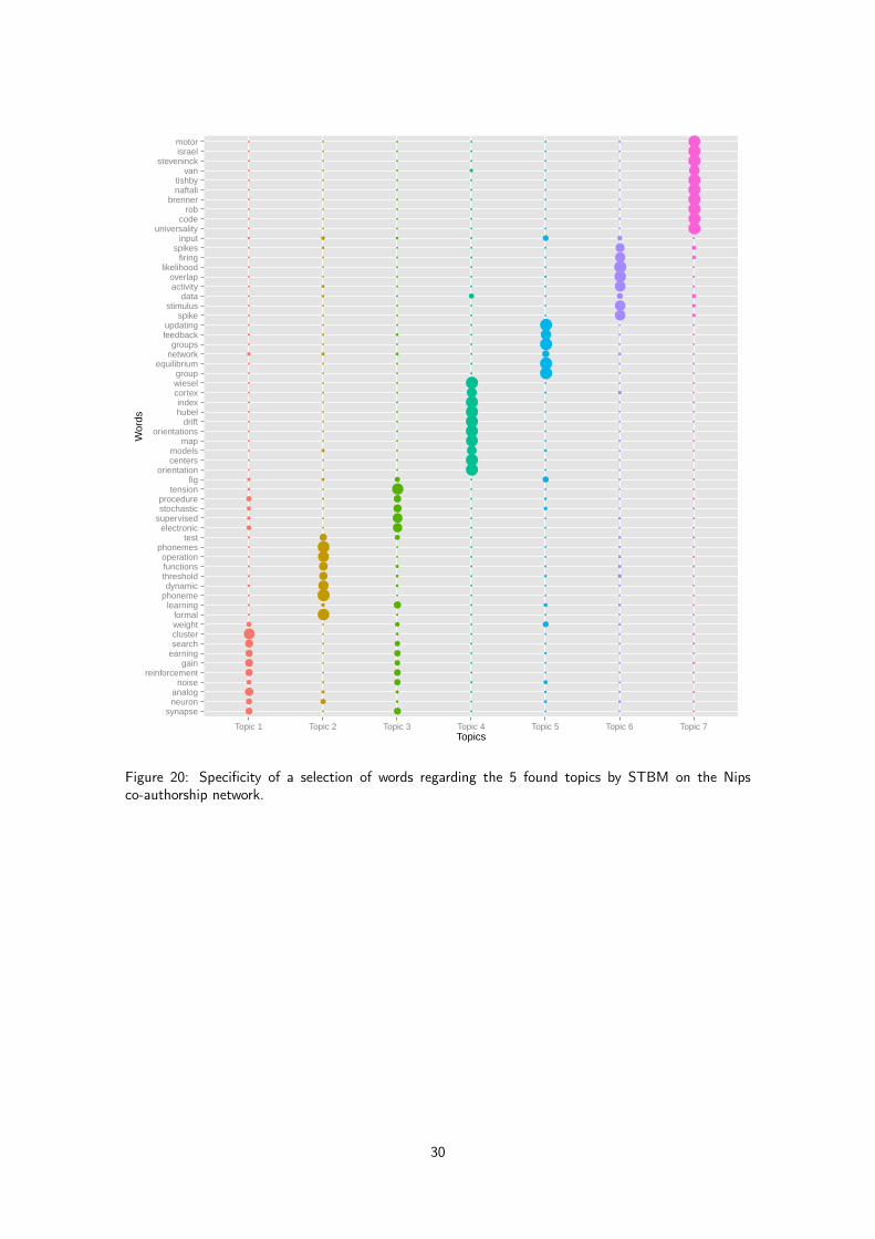
synapseneuronanalog

noisereinforcement

gainearningsearchclusterweightformal

learningphonemedynamic

thresholdfunctionsoperation

phonemestest

electronicsupervisedstochasticprocedure

tensionfig

orientationcentersmodels

maporientations

drifthubelindex

cortexwieselgroup

equilibriumnetworkgroups

feedbackupdating

spikestimulus

dataactivityoverlap

likelihoodfiring

spikesinput

universalitycode

robbrenner

naftalitishby

vansteveninck

israelmotor

Topic 1 Topic 2 Topic 3 Topic 4 Topic 5 Topic 6 Topic 7Topics

Wor

ds

Figure 20: Specificity of a selection of words regarding the 5 found topics by STBM on the Nipsco-authorship network.

30