the stepping stone effects of training contracts: testing
TRANSCRIPT

1
The stepping stone effects of training contracts: testing this hypothesis for the Spanish Labour Market
David Troncoso-Ponce 1 Department of Economics Universidad Pablo de Olavide, Spain J. Ignacio García-Pérez Department of Economics Universidad Pablo de Olavide, Spain
Yolanda Rebollo-Sánz Department of Economics Universidad Pablo de Olavide, Spain
[Very preliminary version]
Abstract
Training contracts is the typical tool to reduce unemployment incidence and to favour job stability for workers with low educational attainment levels. In this paper, we investigate whether training contracts increase the transition rate to regular work. In that case, training contracts may enhance the acquisition and accumulation of skills that outwith their low educational attainment levels. We use longitudinal administrative data of young individuals to estimate a multi-state duration model, applying the “timing of events” approach. To deal with selectivity, the model incorporates both transitions from employment and from unemployment, it allows for competing risk at each state, and unobserved determinants of the transition rates. Our results unambiguously show that training contracts serve as stepping-stones towards regular employment. They reduce the incidence of unemployment and they substantially increase the fraction of low qualified young workers who have regular work within a few years after entry into a training contract, as compared to a situation with other kind of temporary contract. However, these positive effects are only present when the worker moves from one job to another without passing through unemployment. Being fired from a training contract or not finding a new job just after the end of the training contract translates a bad signal to potential employers which makes these workers indistinguishable from the rest of temporary workers.
Keywords Duration analysis; Training contracts; Stepping-stone effect; Unobserved heterogeneity; Temporary contracts
JEL classification C41, J64
1 Corresponding author (David Troncoso).
E-mail address: [email protected]

2
1. Introduction
During the current big recession the unemployment rate has increased across many
European countries and this increase has been particularly high for young workers and
especially for low educated ones. The number of young people out of work in the
OECD area is nearly a third higher than in 2007 and set to rise still further in most of
the countries with already very high unemployment in the months ahead. Youth
unemployment rates exceeded 25% in nine OECD countries at the end of the first
quarter of 2013, including Ireland, Italy, Portugal, Spain and Greece. The sharp increase
in youth unemployment has lead the European Union to send a clear message that more
must be done to provide youth with the skills and help they need to get a better start in
the labour market and progress in their career.
One of the countries where this situation is more dramatic is Spain. According to
Spanish Labour Force Survey (LFS hereafter), there exist important differences in the
unemployment rates by educational attainment levels. At the beginning of the Spanish
economic crisis, by the second quarter of 2008, 31.4% of non-educated young workers
were unemployed (16.9% among all young people). Two years later, in the middle of
the economic crisis this rate raised to 52.1% (31.6%), and six years after (2014) the
unemployment rate reached 56.9% (39.4%). These numbers show the weakness of an
important segment of the Spanish young workforce, and highlight the need to carry out
economic policy actions oriented to solve this important social problem.
As in many European countries, the training or vocational contract has been the
preferred tool within the sets of Active Labour Market Policies (ALMP) in Spain to
facilitate the integration of young workers in the labour market. Especially for low
educated ones which in 2014 still represented 8.1% of the young population. The main
aim of this type of contract is to reduce youth unemployment at the same time that to
improve the skills of young workers. As in other countries, in Spain this contract
implies an agreement between the worker and the firm, in which the latter commits to
invest in workers’ training. However, little is known on whether this contract effectively
help low skill workers to acquire the skills needed to decrease unemployment incidence
and the strong level of job turnover suffer for many low educated workers.
In this paper, we analyze the effect of this active labour market policy, on the
subsequent career development of young individuals. For that purpose, we compare the
labour market career of workers who get a training contract in their first spell of

3
employment relative to the ones who get other temporary contract types at their first
spell of employment. The idea is to test whether the investment in training within the
company has any impact on both employability and job stability for the workers who
benefited from this contract. In particular we analyzed the time needed to find a
permanent job.
An important issue in the ALMP evaluation literature is the difficulty of controlling for
selection biases that may lead to specious positive or negative programme effects. We
use longitudinal administrative data of individuals to estimate a multi-state duration
model, applying the “timing of events” approach (Abbring and Van den Berg, 2003). To
deal with selectivity, the model incorporates transitions from unemployment to
temporary jobs and unobserved determinants of the transition rates.
An important advantage of the dataset we used over survey data is that we have detailed
information of all the employment and unemployment records of each worker since they
first entered the labour market allowing us to trace workers' employment and
unemployment histories over an extended period of time. Using the information
provided by this database we can set up an evaluation exercise. In particular, we
analyzed the labour market history, with a ten years time horizon, of two different
groups: those who began their career through a Training contract –treated workers-, and
those who did it through any other type of temporary contract –control group.
To perform this evaluation analysis we develop a mixed proportional hazards rate model
with multiple states –employment and unemployment, and allowing competing risks for
each state. For the employment state the competing risk are: exit to unemployment; exit
to a temporary contract; and exit to a permanent job. And for the unemployment state
they are: exit to temporary contract and exit to a permanent job. This specification
allows us a precise control of the different labour market transitions an individual can
experience before entering into a permanent contract –which is our absorption state. We
also control for the presence of unobserved heterogeneity. In addition to this, we include
an equation to control for the initial conditions that have an impact on the type of the
employment contract under which the individual has during his first working
experience. Moreover, in this equation, the unobservable factors that influence this
initial condition are considered to be correlated with the unobservable components
affecting both employment and unemployment exit rates in our model.

4
The results obtained show that training contracts notably favour job stability of workers
who start their first spell of employment with this type of contract. These gains in job
stability come from different sources. First, workers who held training contracts have a
lower probability of exit to unemployment during the first year of the contract (10.5%)
than workers who hold other types of temporary contracts (24.7%). Hence they do not
suffer from high job turnover as the “typical” temporary worker does. Second, workers
benefited from a training contract have a much higher probability of having a job-to-job
transition into a permanent contract, than other temporary workers. The differences
found are striking. Although they are almost inexistent after 12 months in the job, by the
end of the second year of the contract, the exit probability to a permanent contract is
30.4% for workers holding a training contract, while it is only 3.9% for workers holding
other kind of temporary contracts. Moreover, at the end of the third year, these
differences get even higher: 44% and 4.7%, respectively. These rates also show the
importance of the treatment duration on the job-to-job rate, and particularly on job
stability, for those hired under this type of contract.
However, these positive outcomes disappear when the worker is not able to get a job-to-
job transition and goes to unemployment after working under a training contract.
Indeed, we get that going through a period of unemployment implies a penalty in the
professional career of all workers in our sample, reflected in reduced and constant exit
rates to a permanent job. Moreover, we observe that this exit rate equals to that of those
who have previously been employed through a Temporary contract (around 5%).
Furthermore, we observe that the exit rate from unemployment to a Temporary job also
equal among those who have just been employed through a Training Contract, and those
who have just been employed under a Temporary one.
The structure of the paper is as follows. Section 2 describes data used and sample
selection. Section 3 reviews existing empirical literature. Section 4 briefly presents a
descriptive analysis of data. The econometric model and the estimation results obtained
are described in Section 5 and 6, respectively. Section 7 shows the importance of
controlling for the presence of unobserved heterogeneity, and Section 8 focuses on the
stepping-stone effect hypothesis. Section 9 presents the results of estimating by
educational levels and discusses the differences obtained. Finally, Section 10 concludes.

5
2. Data
We use administrative longitudinal data from the Spanish Social Security database, the
waves 2011 to 2013 of the Continuous Sample of Working Histories (hereafter CSWH).
The CSWH is compiled annually and every year comprises a 4 percent non-stratified
random sample of the population registered with the Social Security Administration.
Hence, the initial database includes all individuals who came into contact with the
Social Security system -- including both wage and salary workers and recipients of
Social Security benefits, namely, unemployment benefits, disability, survivor pension,
and maternity leave2.
In addition to age, gender, nationality, state of residence (Comunidad Autónoma),
education, and presence of children in the household, the CSWH provides highly
detailed information about the worker's previous job. More specifically, we observe the
dates the employment spell started and ended, the monthly earnings history, the contract
type (permanent versus fixed-term), the occupation and industry, public versus private
sector, and the firm size.3 The CSWH also informs us on the reason for the end of the
employment spell (quit versus layoff), and whether the worker receives unemployment
benefits and the type (UI versus UA). We compute the duration of each unemployment
episode by measuring the time between the end date of the worker’s previous contract
and the start date of the new one.
2.1. Sample selection
The sample finally used in the analysis is defined by the type of active labour market
policy analysed. The training contract is a fixed-term contract (with a maximum
duration of 3 years) addressed to young workers (between 16 and 30 years old) who
lack acknowledged vocational qualification. The aim of this contract is twofold: first,
candidates need to complete some kind of formal educational qualification during the
duration of the contract; second, the skills acquired through qualifications are directly
applied to the hiring company.
2 García-Pérez (2008) and Lapuerta (2010) contain a deep exposition about features of CSWL as well as all necessary techniques to
perform a duration analysis using working lives information.
3 Earnings are deflated using the Spanish CPI (2011, Base).

6
In correspondence with the aim of the training contract, our selected sample is
composed of newly incoming young workers aged between 16 and 30 years old who
started their working career from the year 2000 onwards and for whom their fist
employment spell was a low qualified one4. The strategy followed to analyze the effect
of a Training Contracts in our model is to split sample in two groups of individuals:
those who have been employed through a Training Contract versus those who have been
employed with other type of temporary contract. The purpose of this selection is to get a
sample of workers as homogeneous as possible, for whom the observable differences
are only due to the type of labour contract by which they have start their working career.
In our final sample we have that 24.30% started with a training program, 66.77% started
with another kind of temporary contract and 8.93% started with a Permanent Contract5 .
Table 1 Descriptive statistics
Training Contract Temporary Contract Total spells 20,352 210,070 Completes 19,172 195,723 Censured 1,180 14,347 By Gender Male 64.17 % 63.47 % Female 35.83 % 36.53 % By age 16-19 years old 70.37 % 21.48 % 20-23 years old 26.04 % 38.99 % 24-27 years old 2.70 % 25.27 % 28-30 years old 0.69 % 8.96 % 31 and older 0.20 % 5.29 % By employment duration 1 to 6 months 51.17 % 77.88 % 6 months to 1 year 16.40 % 13.21 % 1 to 2 years 28.47 % 5.87 % 2 to 3 years 3.70 % 1.74 % More than 3 years 0.26 % 1.30 % By qualification level
4 In the CSWL we have information on the qualification level of each employment spell, so we can observe the qualification level
of workers on the job. In this paper, we differentiate four qualification levels: High qualification, Mid-high qualification, Mid-low qualification and Low qualification.
5 We think that this last group might have different observable, and especially unobservable, characteristics. So these can
distinguish them from other workers in the sample. Therefore, to avoid obtaining estimates biased motivated by this fact, we have remove the observations of this group of individuals. However, we do use the information from their first employment spell (that is, the corresponding to the first quarter, since our model defines a quarterly duration) for the identification of Initial Conditions equation defined in the likelihood function of our model. Doing this , we allow that unobservable factors affecting the probability of first access to the labor market through a certain type of labor contract (these are, Training, Temporary or Permanent) are correlated with unobserved components affecting employment exit rates in subsequent jobs through the career path.

7
High qualif. - 2.57 % Mid-High qualif. - 7.78 % Mid-Low qualif. - 39.55 % Low qualif. 100.00 % 50.10 %
3. Related Literature
There exists previous empirical literature that deals with the evaluation of specific
contract regulations as a tool to enhance labour market careers for certain group of
workers. Typically these papers test the stepping-stone effect of different kind of
temporary contracts. For instance, Marloes de Graaf and Van den Berg (2011)
investigate whether temporary work increases the transition rate to regular work. Their
results unambiguously show that temporary jobs serve as stepping-stones towards
regular employment. They shorten the duration of unemployment and they substantially
increase the fraction of unemployed workers who have regular work within a few years
after entry into unemployment, as compared to a situation without temporary jobs.
However, these authors analyzed only transitions from unemployment.
Van den Berg, Holm, and Van Ours (2002) analyze the carrier paths in the medical
profession. They also apply "timing-of-event" approach to analyze the existence of a
stepping-stone effect. The methodology proposed in this article attempts to identify a
causal effect of treatment by controlling for the presence of unobserved heterogeneity
both in the selection to the treatment and in the exit rates analyzed.
However, we have not find any empirical paper that deals with the role of training
contracts on future prospects of workers taking into account on only the short-run
effects but also the medium run effects.
[To be completed]
4. Descriptive analysis
In this section we present the empirical exit rates from employment and unemployment.
To compare like-minded workers, this analysis focuses on the first spell of employment
in their working lives. Specifically, we divide our sample in two different groups: those

8
workers who began their working life through a training contract, and those who did
through another kind of temporary contract.
The competing risks for the exit from employment are: 1) unemployment; 2) temporary
contract; and 3) permanent contract. Figures 1 and 2 show the exists rates from
employment by type of contract and gender. On the other hand, from the unemployed
state, there are two competing risks: exit into a temporary contract or exit into a
permanent job. The exit rates for the unemployment state are presented in Figures 3 and
4.
These Figures show importance differences in the dynamics of the exit rates from
employment for workers holding a training contract relative to workers holding a other
kind of permanent contract. For the first group of workers we have that 40% of men
(and somewhat less for women) who are employed at least two years go directly (job-
to-job) to a Permanent job. And this percentage raises to 50% for those who exhaust the
maximum legal duration of this type of labour contract (36 months). However workers
employed with other temporary contracts, don't experience theses pronounced speaks
neither to a permanent job nor to another Temporary job. And two hazard rate (both to a
Temporary and a Permanent job) remain a pattern practically constant with the duration
spell. It seems that the possible effect of this type of labour contract is being reflected
through the direct transition (job-to-job) from these contract into other Temporary
contract, and especially into a Permanent job.6
6 Much of these direct transitions into a permanent job are experiences within the same firm where the worker has been trained
through the Training Contract. So we think that many of these labor contracts are performing as an investment in human capital and as signaling to the worker within the firm. As a part of our future research agenda, we will introduce in our econometric model a specific risk of these direct transitions (job-to-job) into the same employer. In this paper we focus on a broader objective, that is to analyze transitions into a permanent job without identifying firms of origin and destination.

9
Figure 1 Exit from employment. Kaplan-Meier estimates (first spell). Males.
0.2
.4.6
0 10 20 30 40durmes
CF->U CF->CT CF->CI
0.2
.4.6
0 10 20 30 40durmes
CT->U CT->CT CT->CI
Kaplan Meier : Spell E1
Figure 2 Exit from employment. Kaplan-Meier estimates (first spell). Females.
0.1
.2.3
.4
0 10 20 30 40durmes
CF->U CF->CT CF->CI
0.1
.2.3
.4
0 10 20 30 40durmes
CT->U CT->CT CT->CI
Kaplan Meier : Spell E1

10
Figure 3 Exit from unemployment. Kaplan-Meier estimates (first spell). Males.
0.0
5.1
.15
.2.2
5
0 10 20 30 40durmes
CF->U->CT CF->U->CI
0.0
5.1
.15
.2.2
5
0 10 20 30 40durmes
CT->U->CT CT->U->CI
Kaplan Meier : Spell U1
Figure 4 Exit from unemployment. Kaplan-Meier estimates (first spell). Females.
0.0
5.1
.15
.2
0 10 20 30 40durmes
CF->U->CT CF->U->CI
0.0
5.1
.15
.2
0 10 20 30 40durmes
CT->U->CT CT->U->CI
Kaplan Meier : Spell U1
Hence, this empirical evidence initially points that training contracts might favour the
stability of low educated young workers since they notably increase the transition
probability into a permanent contract. Let's test whether this initial result remains once
we control properly for observed and unobserved characteristics as well as for selection
issues.
5. Econometric model
We have developed a duration model to jointly estimate employment and
unemployment exit rates, using a mixed proportional hazards model with multiple
competing risks depending on the specific state in which the individual is, and
controlling for the presence of unobserved heterogeneity, both for unemployment and

11
employment exits. In addition, we include an equation to control for the initial
conditions that affect the type of labour contract by which the individual had in his first
spell of employment. This equation also allows for unobservable factors that affect this
initial condition to be correlated with unobservable components affecting employment
exit rates in our model.
The different exits depend on the specific state of the individual (if employed or
unemployed). From an employment state, the individual faces three competing risks:
exit to unemployment, to a temporary contract7, or to a permanent contract8. On the
other hand, from the unemployed state, there are two competing risks: exit into a
temporary contract or exit into a permanent job.
To control for the presence of unobserved heterogeneity we estimate our model
following the work of Heckman and Singer (1984), according to which no distribution
for unobserved components should be impose a priori, modelling the distribution of
unobserved heterogeneity nonparametrically. Specifically, we assume the presence of
two different values of heterogeneity, one for employment exit and the other one for the
unemployment's. Also, we allow the existence of a specific heterogeneity component
for each type of exit. And, as mentioned before, given the importance that the literature
gives to the initial conditions problem (see Wooldridge, 2005), we have included an
equation (using a multinomial logit) to control for observable and, specially,
unobservable factors which explain the entry into the labour market of the individual
through a three different types of labour contracts: Training contract, Temporary
contract , or Permanent contract.9 The main purpose of including this equation is to
7 Exit to a Temporary contract (either from employment or from unemployment) also contains the exits to another Training contract.
It is due to small sample reasons, because of the number of observations of exits to a Training Contract is very reduced, since over 60% of employment spells under this type of labor contracts are held on the first work experience in the working lives. Therefore, for reasons of computation, we cannot identify a specific risk in our model to control for exit to a Training Contract. Thus, we have included this specific exits into the rest of Temporary contracts. However, this fact does not prevent us to differentiate them, because we have included explanatory variables to the control for under what type of labor contract is the worker employed, and which type of contract was prior to the current period.
8 In this paper, we consider the event to find a permanent job as an absorption state, by which once the worker has find this type of job, he leaves the sample and its remaining labor history is removed from our estimation sample from that time. 9 In relation to the concept of absorption state explained above, we remove from our estimation sample the remain working lives of
those individuals who begin through a Permanent job. We do this because we believe that workers who begin their working career through a Permanent job may have different features of the rest of our sample, assuming that it could be a possible source of bias in our estimates. Therefore, in our model this group of workers only contributes to the likelihood function through the initial conditions equation. This means eliminating the entire working career of a total of 4,953 individuals who represent 8.93% of all individuals who begin their working lives in our sample. Thus, we guarantee that in our model we are analyzing the effect on exit rates of only two types of labor contract: Training Contract versus other Temporary one.

12
correlate the unobservable component that explains the entry into the labour market
through a particular type of contract (training, temporary or permanent) to the factors,
also unobserved, that affect employment exit rates throughout their future career path.
Unlike Abbring and Van den Berg (2003), we introduce these unobserved components -
that influence the participation in the treatment (defined here as the Training contract)-
in the initial conditions equation. So, doing this, we have not estimating an isolate
causal effect for the treatment, because, although we can guarantee that there's not exist
anticipation effects, in the initial conditions equation there is not exogenous variability
enough. However, we are not trying to estimate a causal effect of the treatment, but the
differential effect in career paths of workers who have been employed under this type of
labour contract.
5.1. Functional form of hazard rates
We estimate a discrete time duration model in intervals defined by quarters. In this
model, we define the exit rate from every specific state towards each one of the
competing risks faced by individuals. This exit rate follows a multinomial logit with the
following general specification:
),,),(),(|( ,,,,,, SSSSSS DST
DSF
DST
DSF
DSDS vzzjxjxjh
S TDS
TDS
TDS
TDS
TDS
TDS
FDS
FDS
FDS
FDS
FDS
DST
DST
DST
DST
DST
DSF
DSF
DSF
DSF
DSF
DS
S
SSSSSSSSSSS
SSSSSSSSSSS
vzjxjzjxj
vzjxjzjxj
,,,,,,,,,,,
,,,,,,,,,,,
)()()()(exp1
)()()()(exp
In each quarter the individual can stay in one of two specific states: employment or
unemployment. This two states define the range of S = {E, U}, i.e. E = employment,
and U = unemployment. The competing risks faced by the individual, which are specific
to each state, define the range of DS. Therefore DE = {U, T, P}, where DE = U implies
exit to unemployment; DE = T implies exit to a Temporary Contract; and DE = P implies
exit to a Permanent Contract. Similarly, defining the two possible risks from the state of
unemployment, we define DU = {T, P}. Therefore DU = T implies exit to a Temporary
Contract; and DU = P implies exit to a Permanent Contract.
We suppose that explanatory variables may affect to exit rates differently if individual is
employed under a Training contract or under a Temporary contract. Therefore we have

13
interacted all these explanatory variables with one of two dummies: a dummy that
identifies if individual is employed under a Training contract (or if he comes from an
employment spell under a Training Contract -for the unemployment state-), and a
dummy that identifies if individual is employed under a Temporary contract (or if he
comes from an employment spell under a Temporary Contract -for the unemployment
state-). Using this type of specification, in practice we are estimating two different
hazard rates, but we may impose a common unobservable heterogeneity component for
two hazard rates.
)(, jxFDS S
and )(, jxTDS S
are two vectors that include time-varying variables specific to
each state and to each competing risk. These vectors include variables such as the
current age 10 of individual in each quarter of the current year, current age squared, the
rate of employment growth, the interaction between the rate of employment growth and
the logarithm of duration spell.
Variables )(, jFDS S
and )(, jTDS S
provide the baseline hazard on exit rates. Specifically,
we introduce a flexible specification of the baseline hazard by defining these variables
as dummies that identifies each quarter in duration spell.
Vectors FDS S
z , and TDS S
z , provide explanatory variables that are not time-varying. These
are: gender of individual, the region, year dummies that allow differentiate periods
before and after the Spanish economic crisis, industry dummies, and variables that
provide information about the past work history of individual: number of temporary
contracts has had to date, a dummy to differentiate if individual have had more than one
Training contract, and the number of unemployment spells.
5.2. Unobserved heterogeneity
As explained above, we have defined unobserved heterogeneity component specific to
each state and to each destination. So, we have several possible values that depend on
the different values for the combination state-destination. In our model, we have defined
SDSv , according to the following structure:
Regarding employment exit rates, since state S = E, and as we defined earlier, we have
three possible destinations specific to state S = E, namely DE = {U, T, P}. Therefore we 10 In our model, we introduce through this variable the difference between the worker's current age in each quarter and the minimum legal age at which individuals can access to a Training Contract (16 years old), and that is the minimum age observed in our sample.

14
define the following unobservable heterogeneity components specific to employment
exit rate:
1. Unobservable heterogeneity component specific to the exit from employment to
unemployment:
EUEUE kv *,,
2. Unobservable heterogeneity component specific to the exit from employment to a
Temporary contract:
ETETE kv *,,
3. Unobservable heterogeneity component specific to the exit from employment to a
Permanent contract:
EPEPE kv *,,
The component E can take two possible values, namely },{ 21EEE . Furthermore,
we normalize the value 1, UEk . So that EUEv , .
With respect to unemployment exit rates, given that state S = U, and as we defined
above, we have two possible competing risks specific to state S = U, given by DU = {T,
P}. Therefore we define the following unobservable heterogeneity components specific
to unemployment exit rate:
1. Unobservable heterogeneity component specific to exit from unemployment to a
Temporary contract:
UTUTU kv *,,
2. Unobservable heterogeneity component specific to exit from unemployment to a
Permanent contract:
UPUPU kv *,,
The component U can take two possible values, namely },{ 21UUU . Furthermore,
we normalize the value 1, TUk . So that UTUv , .

15
5.3. Initial conditions
We have developed the initial conditions equation using a multinomial logit with the
following specification:
S
ISS
ISIS
ISS
ISISISS
ISISS vx
vxvxsh
exp1
exp),|(
In this equation the individual may go into the labour market through a Training
Contract, or do it under a Permanent contract, versus alternative of being employed
under a Temporary Contract. Therefore, we define the range S = {F, P}, where S = F
implies to start their working life under a Training Contract; and S = P implies starting
with a Permanent contract.
As we explained before, the main reason for introducing this equation in our model is to
allow that unobserved components, that affect the type of labour contract under which
the individual starts his working life, are correlated with unobserved factors that affect
employment exit rates throughout their future career path. This is achieved by defining
the unobserved component ISSv .
Thus, we define:
1. Unobservable heterogeneity component specific to those accessing with a Training
contract:
EISF
ISF kv *
2. Unobservable heterogeneity component specific to those accessing with a Permanent
contract:
EISP
ISP kv *
The component E is the same unobserved component we have included in the
employment exit rates specification. Therefore, E can take two possible values,
namely },{ 21EEE . Thus, E is the common unobserved component that makes the
correlation between unobserved factors that affect the type of labour contract under
which the individual starts his working life, and those that affect employment exit rates
throughout their future career path

16
5.4. Likelihood function
Once we have defined functional form of the different exit rates, the initial condition
equation's, and the unobserved heterogeneity structure; we're going to define the
likelihood function of our model.
Following the methodology of Heckman and Singer (1984), the unobserved
heterogeneity is not restricted to a specific probability distribution. Thus, in the
estimation process, we define the likelihood function using four mass-points obtained
for different combinations of two values defined in the range of },{ 21EEE and
},{ 21UUU . To each point-mass is assigned a probability parameter which is
estimated jointly with the rest of the model parameters. The probability parameters
follows a multinomial logit, so that:
3
1
exp1
exp
jj
jj
p
p , for j=1,2,3.
As a result of this combination, we define four different types of individuals: 1) those
who experience shorter episodes of both employment and unemployment; 2) those with
shorter spells of employment and longer spells of unemployment; 3) those with longer
spells of employment and shorter spells of unemployment; and 4) those who experience
longer episodes of both employment and unemployment.
In the model, each mass-point is associated with an estimated probability, and these
build the following four mass-points:
),;,,;,Pr( 111,,1,,1,1,,1,1EIS
PISP
EISF
ISF
EPEPE
ETETE
EUE
UPUPU
UTU kvkvkvkvvkvv
),;,,;,Pr( 222,,2,,1,1,,1,2EIS
PISP
EISF
ISF
EPEPE
ETETE
EUE
UPUPU
UTU kvkvkvkvvkvv
),;,,;,Pr( 111,,1,,1,2,,2,3EIS
PISP
EISF
ISF
EPEPE
ETETE
EUE
UPUPU
UTU kvkvkvkvvkvv
),;,,;,Pr(1 222,,2,,2,2,,2,3214EIS
PISP
EISF
ISF
EPEPE
ETETE
EUE
UPUPU
UTU kvkvkvkvvkvv
The total likelihood function of the model is given by the following expression:
N
i m
T
t
Em
Umitmi
i
lL1
4
1 1
,
And taking the logarithm of this function, we obtain:

17
N
i m
T
t
Em
Umitmi
i
lL1
4
1 1
,loglog
Each of the four mass-point that compose the likelihood function takes the following
expression:
eyIyIyI
PETEUE
yIEmPEPE
yIEmTETE
yIEmUE
Em
Umit
eit
eit
eit
eit
eit
eit hhhkhkhhl
)3()2()1(1
,,,
)3(
,,
)2(
,,
)1(
, 1,
)1()2()1(1
,,
)2(
,,
)1(
, 1e
yIyIPUTU
yIUmPUPU
yIUmTU
uit
uit
uit
uit hhkhh
11111 )2()1(1)2()1(1
eyIyIIS
PISF
yIEm
ISP
ISP
yIEm
ISF
ISF
eit
eit
eit
eit hhkhkh
Due to model complexity and the estimation sample size, composed by quarterly
expanded employment and unemployment spells, we need to program manually first
and second derivatives, because the lack of these would imply that computation time
requirements to get the model parameter estimates would be huge. Moreover, doing
this, we guarantee a better accuracy of parameter estimates, and a more precise standard
errors. Thus, we implement the optimization process by building our own likelihood
function, our gradient vector containing the first derivatives (first order conditions
equations), and our hessian matrix containing the second derivatives (second order
conditions equations). Therefore, the improvement obtained thanks to this model is
outstanding in terms of estimates accuracy and of the programming time required.
Besides the model allows the possibility of estimating sample sizes that otherwise could
not be implemented, thus ensuring the soundness of the coefficients obtained. To carry
out this, we use Stata programming language (see Gould, Pitblado and Sribney, 2006).
The main formulas for gradient vector and hessian matrix can be seen in the Technical
Appendix.

18
6. Estimation results
It is important to know if training contracts are ―stepping stones , using Booth et al.’s
(2002) terminology. If training contracts are not a stepping stone, then the problem
becomes evident because there is a proportion of the population that given they low
educational attainment levels will have strong difficulties to have a stable labour market
career.
In this section we present the estimation results from the econometric model described
in previous section. To show the effect of Training contract on employment and
unemployment exit rates, we build predicted mean hazard rates by calculating the
weighted average of estimated hazard rates from two types of individuals estimated
(type I and type II), where the weights are given by estimated probabilities associated to
each mass-point of the likelihood function defined in our econometric model. Tables A1
y A2 show these predicted mean hazard rates for employment and unemployment exits,
and Figures 5 and 6 plots these rates. Moreover, to see the importance of introducing
unobserved heterogeneity, Tables A3 and A4 show the predicted hazard rates calculated
for each type of individual estimated (type I and type II), and Figures A5 and A6 plots
these rates. Furthermore, the Results Appendix provides tables with the estimation
results. Table A8 shows the coefficients of the initial conditions equation; and Tables
A9 and A10 contain the coefficients from the parameters estimated of employment and
unemployment hazard rates, respectively.
To analyze exit rates we group the explanatory variables into three groups: duration
variables that explain the baseline hazard; variables containing previous labour history
of the individual (in which we will focus in this section); and explanatory variables for
control purposes. In this last group, we have included several control variables: 1) those
relating to individual characteristics: gender, age and nationality; 2) variables to control
for the business cycle, including dummies to differentiate between pre and post
economic crisis period, and the employment growth rate, as well as its interaction with
the logarithm of duration of employment and unemployment spells; 3) regional
dummies to control for the regional effect on hazard rates; 4) variables concerning the
characteristics of the employer: firm size, and the industry in which it has its economic
activity.

19
6.1. Initial conditions
The 66.24% of spells of training contracts in our sample (20.352 spells) occurs right at
the beginning of working life. This is a very important aspect, since our model must
control for the factors that influence workers' selection to the treatment at the beginning
of their careers. This justifies the inclusion of an initial conditions equation, linking the
unobservable factors explaining the choice to treatment with unobservable components
affecting rates from employment.
As explained above, we include this equation to control for the observable and
unobservable factors that explain the individuals began their working life through a
particular labour contract: Training Contract or Permanent Contract, against the
alternative of being employed under a Temporary Contract.
The main objective of this equation is to allow unobservable factors affecting the start
of the working life (through the type of labour contract) are correlated with
unobservable factors that affect employment exit rates, namely },{ 21EEE .
Table A7 shows the explanatory variables included in the initial conditions equation.
These variables include information concerning to individual's personal characteristics
(gender, age, educational level, nationality); characteristics of the employer (size,
economic activity, public or private firm); and regional dummies.
By including this equation in our model, we avoid estimation biases that could lead to
overestimate the possible effect of treatment (Training Contract). Thus, our model takes
into account the unobservable characteristics of workers who first access to the labour
market through a Training contract, against those who enter through another
Temporary contract. Thereby, by introducing in our model heterogeneity components
that affect the selection to treatment (to have a Training contract) and, specially, to
allow this unobservable components are correlated with unobserved factors affecting
employment exit rates, and in particular the probability of finding a permanent job,11 we
are correcting a major source of bias in our econometric estimates.
11 Recall that the unobservable component that affects the selection to the treatment just at the beginning of working life is given by
EISF
ISF kv * , where
E is the unobserved heterogeneity component that affects the exit from employment state.
Therefore, this common factor correlate the unobservable factors that affect the selection to the treatment at the beginning of working life, with unobservable factors affecting employment exit rates throughout the entire working career.

20
6.2. Exit from employment
As we can see in Figure 5 and Table 2, the probability of exiting from a Training
contract shows significant differences depending on the destination state. On the one
hand, we can see that the probability of exiting to unemployment remains relatively
stable throughout the entire duration of the contract, reaching values close to 14% in the
main quarters of spell. 12 However, when we focus on the other competing risks —i.e.
exit to another temporary contract, and exit to a permanent job—, we find that the
employment hazard rates show a quite different pattern. Throughout the duration of
Training contract, there exist only two quarters when treated workers can transit directly
to another job with a very high probability. These peaks are observed in quarter 8 (two
years of contract), and in quarter 12 (the maximum legal duration of Training contract).
Thus, the probability of exiting to another temporary contract in quarter 8 reaches
25.48% (27.17% in quarter 12); and the probability of finding a permanent job in
quarter 8 reaches 33.60% (49.69% in quarter 12). However, in quarters other than 8 and
12, these probabilities decreases to 4-8%, and to 1-3%, for exits to a temporary job and
to a permanent one, respectively.
It seems that workers holding a Training contract have a layoff probability
relatively constant throughout the duration of the Training contract (10-14%), and this is
especially important for those who have employed less than two years: for these treated
workers, the only way out is unemployment. This issue has a particular relevance, since
over 40% of our sample of treated workers —those holding a Training contract— don't
achieve to stay employed at least the two-year. This reflects that there is a high
12 Training Contracts are more stable than the rest of Temporary Contracts. This differential effect varies according to the risk that the individual faces, but for the three possible exits the effect is negative. According to the structure of our model (previously discussed in the previous section), the "clean" effect of having a Temporary contract (other than Training) is included in the two
components of the unobserved heterogeneity, E1 and E
2 (depending on the type of worker). For example for Type 1, the effect of
having a Temporary contract on the exit into unemployment is given by 113.01, -v EUE . Similarly, the effect of having a
Temporary contract on the exit into another Temporary one is given by -1.702(-0.113)* 1kv ETETE 06.5* 1,, . And finally,
the effect of having a Temporary contract on the exit into a Permanent job is given by
772.253.4* 1,, -(-0.113)* 2kv EPEPE . Therefore, to compare the differential effect of having a Training Contract on
employment exit rates, we have to add to these heterogeneity components previously calculated the constant value estimated given by the coefficient called Training contract, taking the following values, depending on the type of output: -1.597 in exit to unemployment; -1.659 to exit to a Temporary contract; and -2.471 to exit to a Permanent job. For example for Type 1, the effect of
having a Training Contract on the exit to unemployment would be given by: 597., 1v UE , namely 1.711.597-0.113- .
The effect of having a Training Contract on the exit to a Temporary one is given by: 659., 1v TE , namely
3.3611.6591.702 . Finally, the effect of having a Training Contract on the exit to a Permanent job is given by:
2.471v PE ,, namely 5.2432.4712.772- .

21
proportion of treated workers for whom the Training contract seems to have no
(immediate) effect on their reemployment rates. However, workers who get to be
employed for at least two years, face to direct reemployment probabilities (via job-to-
job) to a temporary contract, and specially to a permanent job, very high.
This may be a consequence of a potential dual effect triggered by the Training contract,
i.e. the Training contract may be creating a polarized group of treated workers: those
who survive for at least two years (and whose reemployment rates are very high) and
those who cannot be treated long enough to have reemployment probabilities and,
therefore, they exit to unemployment. This might be explained by the fact firms use this
type of contract strategically to recruit workers. It is quite possible that employers may
be using the Training contract as a signalling device: the employer would hire the
worker for the minimum time that the contract requires (i.e. one year), and throughout
the year the employer can evaluate worker productivity.
The firm can hire the worker for the minimum time established by the contract
regulations, which is one year, and depending on employee productivity observed by
the employer throughout this one year period, the firm may decide to renew the
Training contract for six months periods up to three years (which is the maximum legal
contract duration).
This may be explained by the different characteristics (observable, and especially
unobservable) of workers in the company: the more motivated workers could get to stay
employed longer under the Training contract until they reach the legal limit duration of
three years, and the less productive workers would leave out after reaching the
completion (termination) of the contract, without the company's renewed.
Table 2 Predicted mean hazard. Exit from employment (main quarters)
E => U E => T E => P
Training Temporary Training Temporary Training Temporary
Quarter 1 14,26% 32,31% 4,50% 10,05% 0,71% 2,59%
Quarter 4 10,24% 26,42% 6,85% 11,87% 2,31% 5,31%
Quarter 6 14,01% 12,63% 8,11% 5,87% 3,51% 3,28%
Quarter 8 14,95% 13,57% 25,48% 6,51% 33,60% 4,75%
Quarter 12 15,87% 11,23% 27,17% 5,91% 49,69% 4,61%

22
Figure 5 Predicted mean hazard. Exit from employment
0
.1
.2
.3
.4
.5
0 5 10 15(mean) durtrim
E => U E => T E => P
Transition from E: CF
0
.1
.2
.3
.4
.5
0 5 10 15(mean) durtrim
E => U E => T E => P
Transition from E: CT
Previous work experience effect
We focus here on analyzing the effect of past labour history on the employment hazard
rate. To achieve this, we have included in our model a set of variables to control for the
effect that prior labour history accumulated by the individual can have on the exit rates.
Specifically, we have included: 1) a dummy that identifies if individual has been
employed under a Training contract twice or more times 13; 2) a continuous variable that
summarizes the total number of Temporary contracts under the individual has been
employed until the current moment; and 3) a continuous variable that summarizes the
total number of episodes of unemployment 14 that individual has had until the current
moment.
13 This may be due to extension of the current Training Contact within the same firm (whenever duration doesn't exceed the legal maximum of three years). This may also be due to a new Training Contract signed with a different employer. The rules governing this type of contract provides for this possibility, and allows workers to access more of one training contract, whenever worker get to a different qualification to that previously obtained in the previous one.
14 In our sample, unemployment spells include both experiences collecting unemployment benefits (either from a contributory benefit, or a care one), and episodes that mediate between a drop out of a contribution relation with Social Security and the next employment. The latter cases could be called non-employment spells, because we don't observe the individual during period in the MCVL, but we know that neither he is employed nor is collecting any public benefit that involves a contribution relation with Social Security.

23
We can see that work experience has an important effect on the type of transitions, and
especially for those who are employed under a Training contract, especially in the time
it takes to find a permanent job. Thus, according to Table A8, we can observe that for
the individuals who have previously had a Training contract, the probability of find a
job (via job-to-job) raises, and the probability of going to unemployment reduces (the
latter only for employees with a Temporary contract). This effect is much more
pronounced for those who are in a Training contract, for whom we can observe that this
effect is maximum in transitions from a Training contract to a Permanent job.
As Table A8 shows, workers with a Training contract, and previous experience in
another Training contract, have a higher reemployment probability towards another
Temporary contract (0.542), and especially towards a Permanent job (0.730). The effect
of the previous experience variables on reemployment rates is much lower for
Temporary workers (in addition, coefficient associated with the probability of exiting to
a Permanent job is not statistically significant). Although for this group of workers we
can see that the probability of leaving unemployment decreases with prior experience in
a Training Contract.
Then, previous work experience increases the probability of moving into employment,
and reduces the probability of exit to unemployment. And previous episodes of
unemployment seems to have the opposite effect. Furthermore, we observe that all the
variables that summarize the past labour history have a stronger effect on exit rates for
those workers who are employed by a Training contract.
These results show that the positive effects of having had previously a Training contract
on reemployment rates are only observed in those workers who are currently employed
under a Training contract. It seems that to have had a Training contract has no effect on
reemployment rates once the contract has ended, what reinforce our hypothesis through
which this contract does not imply a stepping-stone effect on the future worker's career.
In section 8, we discuss this issue more in depth by analyzing the effect of the most
recent work experience on reemployment hazard rates.

24
6.3 Exit from unemployment
In this section we analyze the exit rates in two groups of workers analyzed: those who
just had a Training contract (treated workers) and those who just had a Temporary one
(control group). As explained above, in our model we define two different risks specific
to unemployment state: exiting to a Temporary contract, and exiting to a Permanent job.
Figure 6 shows the unemployment hazard rates for two groups of workers, and Table 3
contains the same hazard rates for the relevant quarters of the unemployment spell. As
we can see in Figure 6, in contrast to what was observed in the employment hazard
rates, the unemployment hazard rates are quite similar in two groups of workers
analyzed.
As we did in previous section, to capture the effect of duration, we introduce a set of
quarterly dummies, namely quarter 2 to quarter 9. The effect of duration is negative for
exits from both type of labour contracts, except for the exit to a Permanent job for
whose that, previously to the current unemployment state, have been employed under a
Training contract. However this coefficient is not statistically significant. So, as
expected, with increasing duration in the unemployment state, the probability of finding
a job is reducing.
The probability that a treated worker, being unemployed, finds a Temporary contract in
the first quarter of the spell of unemployment is 33.7% (34.8% for workers in the
control group), and this probability is decreases as duration in the state of
unemployment is increasing, with the exception of the quarters 4 and 8, when the exit
rates increases until 29.03% and 24.46%, respectively. However, we can see that
though unemployment hazard rates decreases as duration in unemployment spell is
increasing, however this drop is not too large, since 21.76% of treated workers (15.56%
of control workers) who are unemployed for at least a year and a half —in quarter 6—
find a Temporary job. We are analyzing a sample of young workers, and we think that
for those workers the incidence of negative effects from log term unemployment might
be minimal. On the other hand, if we look at exit rates to a Permanent job, we can see
that the probability of finding a Permanent job is very low, around 3-4% in both groups
of workers, and this rate does not vary with the duration of the unemployment spell.

25
In contrast with what was observed in the employment exit rates for whose workers
with a Training contract, the high peaks of transition to a new job (both to a Temporary,
and specially to a Permanent one) disappear. So, it seems that to go through a period of
unemployment implies a penalty in the professional career of workers in our sample,
reflected in reduced and constant exit rates to a permanent job, around 5%. And we
observe that this exit rates equal to those who have previously been employed through a
Temporary contract (around 5%). Furthermore, we observe that the exit rate from
unemployment to a Temporary job also equal among those who have just been
employed through a Training Contract, and those who have just been employed under a
Temporary one.
Therefore, the possibility of finding a permanent job, by having been employed under a
Training contract, is lost when passing from this type of labour contract to
unemployment. So, we clearly see that the effect of this type of contract occurs through
direct transitions from employment (job-to-job).
Table 3 Predicted mean hazard. Exit from unemployment (main quarters)
U => T U => P
Training Temporary Training Temporary
Quarter 1 33,74% 34,83% 3,80% 4,25%
Quarter 2 25,49% 25,19% 3,06% 3,35%
Quarter 4 29,03% 32,20% 3,23% 3,43%
Quarter 6 21,76% 15,56% 2,15% 3,25%
Quarter 8 24,46% 23,15% 4,07% 4,46%

26
Figure 6 Predicted mean hazard. Exit from unemployment
0
.1
.2
.3
.4
0 2 4 6 8 10(mean) durtrim
U -> T U -> P
U -> E (previous Training)
0
.1
.2
.3
.4
0 2 4 6 8 10(mean) durtrim
U -> T U -> P
U -> E (previous Temporary)
Previous work experience effect
In the unemployment equation, we have included a set of explanatory variables for
analyzing the effect that the previous employment history has on the probability of
leaving unemployment state. These variables include information on: 1) whether the
worker
previously had one or more Training contracts; 2) the number of Temporary contracts
the worker has had until the current unemployment spell; and 3) the number of
unemployment episodes the worker has had until the current unemployment spell.
Our estimates show that previous experience in a Training contract increases the
probability of leaving unemployment. For workers who have had only one episode of
Training contract, the effect on the exit toward a Temporary job is practically the same
in both groups of workers: 0.274 and 0.265 for treated and control workers,
respectively. However, for treated workers the effect on the probability of finding a
Permanent job is negative (although the associated coefficient is not statistically
significant) while for workers in the control group, this effect is positive (0.349) and
statistically significant.
27
Again, by analyzing the similarities in the unemployment exit rates of two groups of
workers, our hypothesis, by which the potential treatment effect disappears once the
Training contract ends (i.e. non-exactly stepping-stone effect), is gaining strength.
Although these results must be interpreted with carefully, since, as we discussed above,
in this section we are analyzing workers who didn't achieve a direct transition from the
treatment —Training contract— to another job. Therefore, we may be observing a
group of "bad" workers, i.e. a group of treated workers less productive that have failed
in getting a matching with the employer while they was hired with a Training contract.
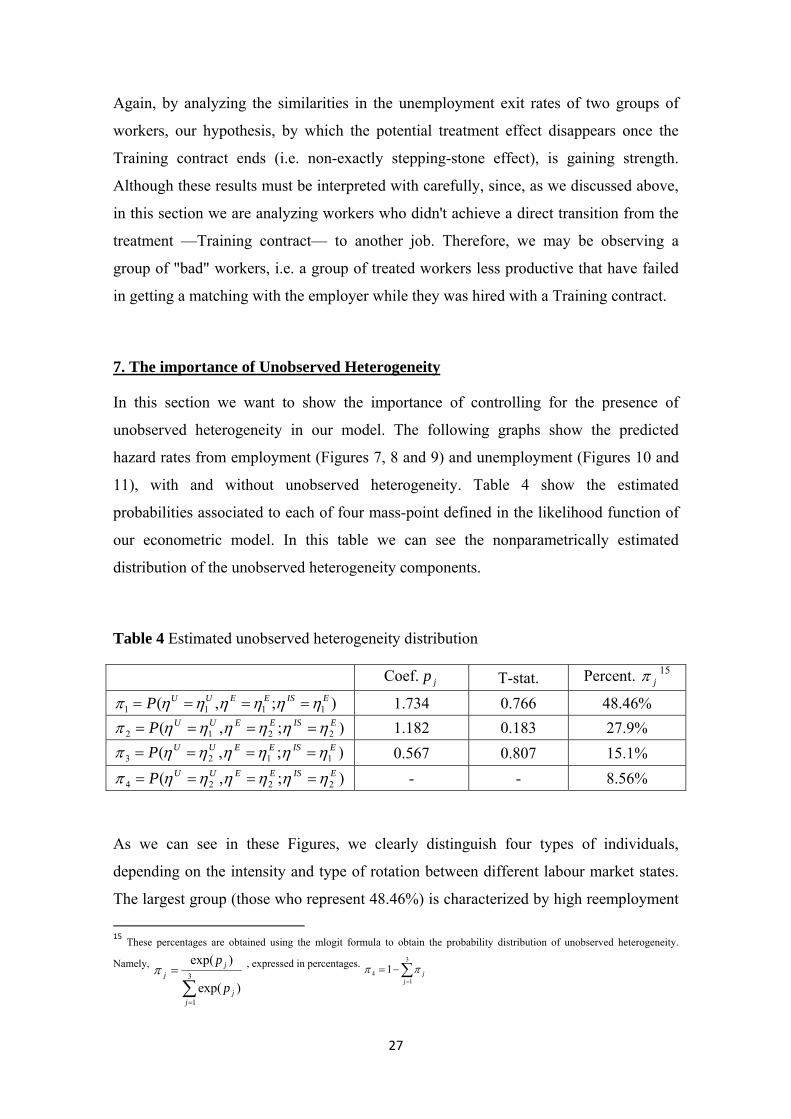
7. The importance of Unobserved Heterogeneity
In this section we want to show the importance of controlling for the presence of
unobserved heterogeneity in our model. The following graphs show the predicted
hazard rates from employment (Figures 7, 8 and 9) and unemployment (Figures 10 and
11), with and without unobserved heterogeneity. Table 4 show the estimated
probabilities associated to each of four mass-point defined in the likelihood function of
our econometric model. In this table we can see the nonparametrically estimated
distribution of the unobserved heterogeneity components.
Table 4 Estimated unobserved heterogeneity distribution
Coef. jp T-stat. Percent. j 15
);,( 1111EISEEUUP 1.734 0.766 48.46%
);,( 2212EISEEUUP 1.182 0.183 27.9%
);,( 1123EISEEUUP 0.567 0.807 15.1%
);,( 2224EISEEUUP - - 8.56%
As we can see in these Figures, we clearly distinguish four types of individuals,
depending on the intensity and type of rotation between different labour market states.
The largest group (those who represent 48.46%) is characterized by high reemployment
15 These percentages are obtained using the mlogit formula to obtain the probability distribution of unobserved heterogeneity.
Namely,
3
1
)exp(
)exp(
jj
jj
p
p , expressed in percentages.
3
14 1
jj

28
rates (via job-to-job), as well as high exit rates from unemployment: when they go into
an unemployment episode, also experience a quick exit from this state to a new job.
This is the group with the desired work behaviour, since most of them come directly
from one job to another (via job-to-job), and once unemployed find a new job quickly.
For these, treatment (having a Training contract) has a great effect on reemployment
rates (via job-to-job) from the Training contract to another Temporary contract (the
27.48% of those who carry at least 8 quarters Training employees with leave to a
Temporary contract, and this rate rises to 28.09% for those who exhaust treatment).
This effect is even higher when we analyze reemployment rates (via job-to-job) from
Training contract to a Permanent job: 33.75% of those holding a Training contract at
least 8 quarters find a Permanent job, and 48.20% of workers who exhaust treatment do.
There is another group of workers, who represent 8.56% of sample. These workers
experience high reemployment rates from treatment, therefore Training contract has a
positive effect on their reemployment rates. But if they go from Training contract into
an unemployment episode, the probability of find a new job is quite lower than for the
previous group described earlier. Furthermore, we observe that once unemployed, the
probability of finding a Permanent job is practically zero and it does not depend on the
duration of unemployment spell.
In fact, as we can see in Figures 10 and 11, the predicted unemployment hazard rates
estimated without unobserved heterogeneity mainly describe the behaviour of 36.46%
of sample (as result of adding the percentages %9.272 and %56.84 ). Thus, if
we had not considered the presence of unobserved heterogeneity in our model, we
would have been unable to identify the remaining 63.54% of individuals whose work
behaviour differs from the rest, and for whom the treatment seems to have no effect on
reemployment rates. This would had implied a clear source of bias in our estimates.
8. A non exactly stepping-stone effect In Section 6, we have seen that unemployment hazard rates of both treated and control
workers tend to be very similar. This may can show that treated workers who don't
achieve a direct transition —from the Training contract to another Temporary contract,
or to a Permanent one— and therefore go into unemployment state, loose the higher
opportunities of finding a Permanent job, provided by the Training contract. Thus, upon

29
at unemployment state, treated workers have almost the same probabilities of finding a
new job (temporary or permanent) than workers in the control group. Figures 10 and 11
show the similarity of the probabilities of leaving unemployment among those who
have just had a Training contract, and those who have been employed with a Temporary
one
The main aim of this paper is to investigate whether the Training contract imply (or not)
a stepping-stone effect on the prospect labour career of treated workers. To do this, we
have include a set of explanatory variables in the employment equation that focus on
information about the most recent past labour experience of workers. We define this set
of variables only for the workers of control group (i.e. for workers who are currently
employed under a Temporary contract). By doing this, we want to analyze if the
potential treatment effects disappear when the treatment ends (i.e. when the Training
contract finishes).
This set of variables includes: 1) A dummy variable that takes value one if the
temporary worker comes just from an unemployment spell; 2) A dummy variable that
takes value one if the temporary worker comes just from a Training contract with a
duration between one and three quarters; 3) A dummy variable that takes value one if
the temporary worker comes just from a Training contract with a duration between four
and six quarters; and 4) A dummy variable that takes value one if the temporary worker
comes just from a Training contract with a duration between 7 and 12 quarters.
By analyzing the estimated coefficients associated to these variables, we highlight the
following results: Firstly, temporary workers who come from an unemployment spell
have a higher probability of go back to unemployment state (the associated coefficient
is 0.168 and is statistically significant), and have a lower probability of exiting directly
to another job, both to a Temporary contract (-0.038), and to a Permanent job (-0.0763).
Secondly, temporary workers who come from a Training contract have a lower
probability of exiting both to an unemployment spell, and to another job.
As Table A8 shows, as duration of previous Training contract increases, the probability
of exiting to unemployment decreases, what may reflects that duration of the treatment
affects substantially to transitions from temporary employment to unemployment.
Furthermore, the probability of finding a temporary job is significantly affected by the

30
duration of treatment. Again, we find that coefficients associated —to the exit toward a
temporary job— become more negative as the duration of treatment increases. This is a
striking result since we would expect the opposite sign for these last coefficients (i.e.
that the probability of finding a new job was positively correlated with the duration of
treatment).

31
Figure 7 Employment hazard rates (E => U) , without and with unobserved heterogeneity (by type of individual)
0
.1
.2
.3
.4
0 5 10 15(mean) durtrim
Without U.H.
With U.H. (Type I)
With U.H. (Type II)
Transition from CF => U
0
.1
.2
.3
.4
0 5 10 15(mean) durtrim
Without U.H.
With U.H. (Type I)
With U.H. (Type II)
Transition from CT => U
Figure 9 Employment hazard rates (E => P) , without and with unobserved heterogeneity (by type of individual)
0
.2
.4
.6
0 5 10 15(mean) durtrim
Without U.H.
With U.H. (Type I)
With U.H. (Type II)
Transition from CF => P
0
.2
.4
.6
0 5 10 15(mean) durtrim
Without U.H.
With U.H. (Type I)
With U.H. (Type II)
Transition from CT => P
Figure 8 Employment hazard rates (E => T) , without and with unobserved heterogeneity (by type of individual)
0
.1
.2
.3
0 5 10 15(mean) durtrim
Without U.H.
With U.H. (Type I)
With U.H. (Type II)
Transition from CF => T
0
.1
.2
.3
0 5 10 15(mean) durtrim
Without U.H.
With U.H. (Type I)
With U.H. (Type II)
Transition from CT => T

32
Figure 10 Unemployment hazard rates (U => T) , without and with unobserved heterogeneity (by type of individual)
.1
.2
.3
.4
0 2 4 6 8 10(mean) durtrim
Without U.H.
With U.H. (Type I)
With U.H. (Type II)
U => T (previous Training)
.1
.2
.3
.4
0 2 4 6 8 10(mean) durtrim
Without U.H.
With U.H. (Type I)
With U.H. (Type II)
U => T (previous Temporary)
Figure 11 Unemployment hazard rates (U => P) , without and with unobserved heterogeneity (by type of individual)
0
.02
.04
.06
.08
0 2 4 6 8 10(mean) durtrim
Without U.H.
With U.H. (Type I)
With U.H. (Type II)
U => P (previous Training)
0
.02
.04
.06
.08
0 2 4 6 8 10(mean) durtrim
Without U.H.
With U.H. (Type I)
With U.H. (Type II)
U => P (previous Temporary)

33
9. Estimation by educational levels
In this section we investigate whether the educational level (differences) achieved by
workers in our sample may have a significance influence on the treatment effect.
Therefore, we have split our sample according to three educational levels, and we have
estimated the econometric model in each of these three subsamples.
We define the following three educational levels: 1) Low education (this subsample
consists of workers with incomplete primary education); 2) Mid education (this
subsample consists of workers with complete primary education and workers with the
first stage of secondary education); and 3) vocational training and bachelor degree (this
subsample consists of workers with a vocational training degree and workers with a
bachelor degree).
Tables 5 and 6 show, for the main quarters of the spell, the predicted employment and
unemployment hazard rates, respectively; and Figures 12 and 17 plot theses hazard rates
evaluated in the sample mean. 16As we can see in Table 5, employment hazard rates
show important differences by educational levels. The results show that treated workers
with mid education and workers with a vocational or bachelor degree have a much
lower probability of exiting to unemployment; have a lightly high probability of exiting
to another Temporary contract; and have a much higher probability of finding a
Permanent job.
The differences are striking. With respect to the transitions from the Training contract to
unemployment, in quarter 6 this probability for workers with a vocational or bachelor
degree is 8.5% (10.95% in quarter 8); for workers with mid education is 14.1% (16.56%
in quarter 8); and for workers without education is 17.21% (16.24% in quarter 8).
If we focus on transitions from the Training contract to a Permanent job, we see that for
example in quarter 8, the probability of finding a Permanent job for workers with a
vocational or bachelor degree is 33% (50.21% in quarter 12); for workers with mid
education is 34.22% (52.85% in quarter 12); and for workers without education is
28.63% (43.63% in quarter 12).
16 All these estimation results are available upon request.

34
Table 5 Predicted mean hazard, by educational level. Exit from employment (main quarters)
Without Education Low Education Vocational training or
bachelor degree
E => U Training Temporary Training Temporary Training Temporary
Quarter 1 13,80% 31,84% 13,59% 30,92% 12,85% 33,87%
Quarter 4 10,96% 26,77% 10,44% 26,42% 7,86% 26,62%
Quarter 6 17,21% 14,29% 14,10% 12,21% 8,50% 11,54%
Quarter 8 16,24% 13,21% 16,56% 12,56% 10,95% 14,79%
Quarter 12 19,93% 13,10% 13,00% 11,20% 13,51% 7,85%
Without Education Low Education Vocational training or
bachelor degree
E => T Training Temporary Training Temporary Training Temporary
Quarter 1 3,66% 9,42% 4,98% 10,47% 4,69% 10,26%
Quarter 4 6,04% 11,51% 7,28% 12,63% 5,80% 11,13%
Quarter 6 7,26% 5,73% 7,98% 6,26% 7,66% 5,61%
Quarter 8 25,52% 6,16% 25,62% 7,01% 23,53% 6,66%
Quarter 12 26,87% 6,66% 29,25% 6,88% 26,62% 5,08%
Without Education Low Education Vocational training or
bachelor degree
E => P Training Temporary Training Temporary Training Temporary
Quarter 1 0,54% 2,06% 0,78% 2,66% 0,89% 3,28%
Quarter 4 1,70% 4,61% 2,57% 5,27% 2,14% 6,02%
Quarter 6 2,86% 2,48% 3,41% 3,43% 3,37% 3,91%
Quarter 8 28,63% 3,87% 34,22% 4,60% 33,00% 6,14%
Quarter 12 43,63% 3,60% 52,82% 4,29% 50,21% 7,01%
Table 6 Predicted mean hazard, by educational level. Exit from unemployment (main quarters)
Without Education Low Education Vocational training or
bachelor degree
U => T Training Temporary Training Temporary Training Temporary
Quarter 1 33,10% 34,24% 35,18% 36,49% 34,55% 33,16%
Quarter 2 26,20% 25,69% 26,92% 27,09% 24,48% 23,38%
Quarter 4 24,54% 25,96% 26,35% 29,04% 45,10% 42,06%
Quarter 6 22,05% 14,85% 22,54% 17,72% 24,10% 15,09%
Quarter 8 20,38% 19,59% 20,92% 20,88% 42,13% 29,81%
Without Education Low Education Vocational training or
bachelor degree
U => P Training Temporary Training Temporary Training Temporary
Quarter 1 2,71% 3,30% 3,49% 4,55% 4,81% 5,05%
Quarter 2 1,96% 2,80% 3,00% 3,78% 4,18% 3,84%
Quarter 4 3,41% 2,24% 2,02% 3,17% 4,49% 5,58%
Quarter 6 1,64% 1,92% 1,89% 4,34% 3,35% 4,34%
Quarter 8 3,60% 2,59% 3,97% 5,20% 4,27% 6,68%

35
0
.1
.2
.3
.4
0 5 10 15(mean) durtrim
E -> U E -> T E -> P
Transition from E: CF
0
.1
.2
.3
.4
0 5 10 15(mean) durtrim
E -> U E -> T E -> P
Transition from E: CT
Low Education
Figure 12 Exit from employment. Low education
0
.1
.2
.3
.4
.5
0 5 10 15(mean) durtrim
E -> U E -> T E -> P
Transition from E: CF
0
.1
.2
.3
.4
.5
0 5 10 15(mean) durtrim
E -> U E -> T E -> P
Transition from E: CT
Mid Education
Figure 13 Exit from employment. Mid education
0
.1
.2
.3
.4
.5
0 5 10 15(mean) durtrim
E -> U E -> T E -> P
Transition from E: CF
0
.1
.2
.3
.4
.5
0 5 10 15(mean) durtrim
E -> U E -> T E -> P
Transition from E: CT
Vocational Education
Figure 14 Exit from employment. Vocational and bachelor degree

36
0
.1
.2
.3
.4
0 2 4 6 8 10(mean) durtrim
U -> T U -> P
U -> E (previous CF)
0
.1
.2
.3
.4
0 2 4 6 8 10(mean) durtrim
U -> T U -> P
U -> E (previous CT)
Low Education
Figure 15 Exit from unemployment. Low education
0
.1
.2
.3
.4
0 2 4 6 8 10(mean) durtrim
U -> T U -> P
U -> E (previous CF)
0
.1
.2
.3
.4
0 2 4 6 8 10(mean) durtrim
U -> T U -> P
U -> E (previous CT)
Mid Education
Figure 16 Exit from unemployment. Mid education
0
.1
.2
.3
.4
.5
0 2 4 6 8 10(mean) durtrim
U -> T U -> P
U -> E (previous CF)
0
.1
.2
.3
.4
.5
0 2 4 6 8 10(mean) durtrim
U -> T U -> P
U -> E (previous CT)
Vocational Education
Figure 17 Exit from unemployment. Vocational and bachelor degree

37
10. Concluding Remarks
Training contracts have become a major form of active labour market policy to reduce the
unemployment incidence of low educated young workers and to enhance their chances of
entering into a regular work. If training contracts are not a stepping stone, then the problem
becomes evident because there is a proportion of the population that, given they low
educational attainment level, will have strong difficulties to have a stable labour market
career. Available evidence about whether these contracts are a stepping stone to a permanent
employment are not common since the empirical literature has mostly focused on the role of
temporary contracts of any kind as a device to favour future regular employment. However,
training contracts are not the typical temporary contract since benefited workers may acquire
formal education and training during the life of the contract. Hence, they deserve special
attention.
For testing the stepping-stone hypothesis, we analyse a sample of low educated young
employees (16-30 years old) for the period 2000-2012, obtained from Spanish administrative
Social Security records, and apply a mixed proportional hazards rate model with multiple
states –employment and unemployment– facing multiple competing risks, and controlling for
the presence of unobserved heterogeneity.
The results obtained show that 30% of young people hired at least for two years under this
contract find a permanent job immediately after the training contract (without any
unemployment period in between). This rate increases almost to 50% for those who complete
the full duration of the contract, which shows the importance of the treatment duration on the
job-to-job rate for those hired under this type of contract. Hence, it seems that in Spain, some
firms make use of this type of contract as a signalling device—once trained and qualified,
these employees are reintroduced into their production process.
However, it is not clear the presence of a stepping-stone effect, since the treatment effect is
reflected in the reemployment rates (directly from the Training contract to another Temporary
contract, and especially, to a Permanent job), but this effect seems to disappear once treatment
has ended (i.e. once the Training contract has concluded). That is, if throughout the duration
of the Training contract the worker fails, and hence, he does not get a new job before the end
of contract; once the treatment is finished, and he goes into an unemployment episode, the
probability of finding a job will be practically the same for anyone who has not previously

38
received the treatment. Therefore, according to the results obtained, we can argue that
Training contract has a positive effect on employment rates immediately after receiving the
treatment, but we cannot conclude that Training contract involve a stepping-stone effect in
working career of individuals treated.
References Abbring, Jaap H. and Gerard J. Van den Berg, (2003): "The nonparametric identification of treatment effects in duration models", Econometrica, Vol. 71, No. 5, 1491-1517. García-Pérez, J.I. and Muñoz-Bullón, F. (2011): "Transitions into Permanent Employment in Spain: An Empirical Analysis for Young Workers", The British Journal of Industrial Relations, Vol 49(1), pp. 103-143.
Gould, W., Pitblado, J. and Sribney, W. (2006), Maximum Likelihood Estimation with Stata, Third Edition, Stata Press. Heckman, J. J. and Singer, B. (1984): “A Method for Minimizing the Impact of the Distributional Assumptions in Econometric Models for Duration Data”, Econometrica, Vol. 52, pp. 271–320. Heckman, J.J. and B.E. Honoré (1989): "The identifiability of the competing risk models", Biometrika, 76, 325-330.
Honoré, B.E. (1993): "Identification results for duration models with multiple spells", Review of Economic Studies, 60, 241-246.
Kaplan, E.L. and Meier, P. (1958): “Nonparametric estimation from incomplete observations”, Journal of the American Statistical Association, 53, pp. 457-481. Lancaster, T. (1990), The econometric analysis of transition data, Cambridge University Press, Cambridge. Marloes de Graaf-Zijl, Gerard J. van den Berg, Arjan Heyma (2011): "Stepping stones for the unemployed: the effect of temporary jobs on the duration until (regular) work", Journal of Population Economics, 24:107–139. Rebollo, Yolanda (2011): "Landing a permanent contract in Spain: Do job interruptions and employer diversification matter?", The Manchester School, Vol. 79, No. 6, pp. 1197-1236.

39
Van den Berg, G.J. (1999): "Duration models: specification, identification and multiple durations", in J.J. Heckman and E. Leamer (eds.), Handbook of Econometrics, Volume V, North-Holland, Amsterdam.
Wooldridge, J. (2005): "Simple solutions to the initial conditions problem for dynamic, nonlinear panel data models with unobserved heterogeneity", Journal of Applied Econometrics 20(1): 39-54.

40
Results Appendix
Table A1 Predicted mean hazard. Exit from employment
CF -mean hazard- CT -mean hazard- Duration of spell
(in quarters) E => U E => T E => P E => U E => T E => P 1 14,26% 4,50% 0,71% 32,31% 10,05% 2,59%
2 14,26% 4,50% 0,71% 32,31% 10,05% 2,59%
3 4,80% 3,17% 0,63% 20,33% 8,71% 3,07%
4 10,24% 6,85% 2,31% 26,42% 11,87% 5,31%
5 4,04% 3,86% 1,19% 13,98% 6,28% 2,80%
6 14,01% 8,11% 3,51% 12,63% 5,87% 3,28%
7 2,77% 3,39% 2,16% 12,21% 5,29% 2,90%
8 14,95% 25,48% 33,60% 13,57% 6,51% 4,75%
9 3,10% 4,41% 4,12% 9,28% 4,78% 2,83%
10 3,10% 4,41% 4,12% 9,28% 4,78% 2,83%
11 3,10% 4,41% 4,12% 9,28% 4,78% 2,83%
12 15,87% 27,17% 49,69% 11,23% 5,91% 4,61%
13 0,00% 0,00% 0,00% 7,02% 4,68% 3,44%
Table A2 Predicted mean hazard. Exit from unemployment
CF -mean hazard- CT -mean hazard- Duration of spell
(in quarters) U => T U => P U => T U => P 1 33,74% 3,80% 34,83% 4,25%
2 25,49% 3,06% 25,19% 3,35%
3 30,21% 3,15% 29,87% 3,38%
4 29,03% 3,23% 32,20% 3,43%
5 19,08% 3,87% 18,22% 3,32%
6 21,76% 2,15% 15,56% 3,25%
7 23,64% 3,73% 19,03% 3,56%
8 24,46% 4,07% 23,15% 4,46%
9 18,31% 5,53% 14,60% 4,43%

41
Table A3 Predicted hazard, by type of individual. Exit from employment
CF -Type I- CT -Type I- CF -Type II- CT -Type II- Duration of spell (in quarters) E => U E => T E => P E => U E => T E => P E => U E => T E => P E => U E => T E => P
1 14,27% 5,15% 0,87% 31,84% 11,38% 3,15% 14,24% 3,36% 0,43% 33,13% 7,74% 1,61%
2 14,27% 5,15% 0,87% 31,84% 11,38% 3,15% 14,24% 3,36% 0,43% 33,13% 7,74% 1,61%
3 4,82% 3,64% 0,77% 20,08% 9,88% 3,74% 4,77% 2,35% 0,37% 20,76% 6,68% 1,90%
4 10,17% 7,80% 2,82% 25,80% 13,35% 6,43% 10,35% 5,19% 1,41% 27,51% 9,30% 3,36%
5 4,04% 4,43% 1,47% 13,88% 7,15% 3,43% 4,02% 2,88% 0,72% 14,15% 4,77% 1,72%
6 13,85% 9,20% 4,28% 12,53% 6,68% 4,01% 14,29% 6,21% 2,17% 12,79% 4,46% 2,01%
7 2,77% 3,88% 2,65% 12,14% 6,03% 3,55% 2,77% 2,54% 1,30% 12,32% 4,00% 1,77%
8 13,11% 26,39% 38,04% 13,41% 7,38% 5,79% 18,16% 23,90% 25,87% 13,86% 4,99% 2,94%
9 3,09% 5,02% 5,04% 9,24% 5,46% 3,47% 3,14% 3,34% 2,51% 9,35% 3,61% 1,72%
10 3,09% 5,02% 5,04% 9,24% 5,46% 3,47% 3,14% 3,34% 2,51% 9,35% 3,61% 1,72%
11 3,09% 5,02% 5,04% 9,24% 5,46% 3,47% 3,14% 3,34% 2,51% 9,35% 3,61% 1,72%
12 13,10% 26,85% 54,13% 11,12% 6,72% 5,62% 20,69% 27,72% 41,97% 11,44% 4,52% 2,84%
13 0,00% 0,00% 0,00% 6,99% 5,33% 4,21% 0,00% 0,00% 0,00% 7,09% 3,54% 2,10%

42
Table A4 Predicted hazard, by type of individual. Exit from unemployment
CF -Type I- CT -Type I- CF -Type II- CT -Type II- Duration of spell (in quarters) U => T U => P U => T U => P U => T U => P U => T U => P
1 37,10% 4,82% 38,20% 5,38% 22,89% 0,53% 23,93% 0,60%
2 28,33% 3,89% 28,00% 4,26% 16,30% 0,40% 16,14% 0,43%
3 33,40% 3,99% 33,02% 4,28% 19,89% 0,42% 19,69% 0,45%
4 32,14% 4,10% 35,50% 4,34% 19,00% 0,43% 21,54% 0,47%
5 21,32% 4,92% 20,40% 4,22% 11,86% 0,48% 11,19% 0,41%
6 24,32% 2,73% 17,46% 4,14% 13,46% 0,27% 9,40% 0,39%
7 26,29% 4,74% 21,27% 4,53% 15,06% 0,48% 11,78% 0,44%
8 27,17% 5,17% 25,72% 5,66% 15,73% 0,53% 14,84% 0,58%
9 20,40% 7,02% 16,37% 5,64% 11,54% 0,70% 8,90% 0,54%

43
Figure A5 Predicted mean hazard, by type of individual. Exit from employment
0
.2
.4
.6
0 5 10 15(mean) durtrim
E => U E => T E => P
Transition from E : CF -Type I-
0
.2
.4
.6
0 5 10 15(mean) durtrim
E => U E => T E => P
Transition from E : CT -Type I-
0
.2
.4
.6
0 5 10 15(mean) durtrim
E => U E => T E => P
Transition from E : CF -Type II-
0
.2
.4
.6
0 5 10 15(mean) durtrim
E => U E => T E => P
Transition from E : CT -Type II-

44
Figure A6 Predicted mean hazard, by type of individual. Exit from unemployment
0
.1
.2
.3
.4
0 2 4 6 8 10(mean) durtrim
U -> T U -> P
U -> E (previous Training): Type I
0
.1
.2
.3
.4
0 2 4 6 8 10(mean) durtrim
U -> T U -> P
U -> E (previous Temporary): Type I
0
.1
.2
.3
.4
0 2 4 6 8 10(mean) durtrim
U -> T U -> P
U -> E (previous Training): Type II
0
.1
.2
.3
.4
0 2 4 6 8 10(mean) durtrim
U -> T U -> P
U -> E (previous Temporary): Type II

45
Table A7 Initial conditions
Training Permanent
Personal characteristics (dummies)
Female (=1) 0.330*** -0.143***
Age 20-23 -0.864*** 0.280***
Age 24-30 -2.576*** 0.470***
Economic Immigrant -0.682*** 0.351***
Firm characteristics (dummies)
Public firm 2.390*** -3.469***
Firm size without info. 2.890*** -0.241***
Firm size small (1-2 workers) 2.535*** 0.223***
Economic sector (dummies)
Industry or Construction sectors 1.063*** 0.0836*
Commercial or Hospitality sectors 0.783*** 0.654***
Regional dummies
Andalucia 1.038*** -0.743***
Aragon 0.0346 -0.258**
Asturias 1.524*** -0.497***
Baleares 0.0446 -0.685***
Canarias -0.0795 -0.306***
Cantabria 0.809*** -0.933***
Castilla La Mancha 0.550*** -0.275***
Castilla Leon 0.413*** -0.460***
Valencia 0.428*** -0.325***
Extremadura 1.284*** -0.499***
Galicia 1.512*** -0.590***
Madrid 0.756*** 0.0994*
Murcia 0.643*** 0.0421
Navarra 0.373*** -0.470***
Pais Vasco 0.464*** -0.409***
Observations 49,484

46
Table A8 Exit from employment
Worker currently employed under a Training contract Worker currently employed under a Temporary contract
E => U E => T E => P E => U E => T E => P
Baseline hazard Baseline hazard
Quarter 3 -1.215*** -0.476*** -0.250** Quarter 3 -0.673*** -0.353*** -0.0395 U1 -0.786***
Quarter 4 -0.332*** 0.422*** 1.184*** Quarter 4 -0.225*** 0.145*** 0.699*** (0.0209)
Quarter 5 -1.383*** -0.273*** 0.402*** Quarter 5 -1.172*** -0.806*** -0.257*** U2 -1.546***
Quarter 6 0.0625 0.672*** 1.687*** Quarter 6 -1.291*** -0.891*** -0.118** (0.0365)
Quarter 7 -1.767*** -0.411*** 0.985*** Quarter 7 -1.342*** -1.013*** -0.258*** E
1 -0.113***
Quarter 8 1.182*** 2.900*** 5.045*** Quarter 8 -1.179*** -0.747*** 0.295*** (0.0230)
Quarters 9-11 -1.617*** -0.111 1.671*** Quarters 9-11 -1.659*** -1.157*** -0.326*** E2 -0.143***
Quarter 12 2.516*** 4.252*** 6.732*** Quarter 12 -1.408*** -0.883*** 0.224** (0.0308)
Quarter 13 -1.959*** -1.199*** -0.153 UPk 3.282***
Current spell Current spell (0.113)
Training contract (=1) -1.597*** -1.659*** -2.471*** Part time job (=1) -0.00211 0.0823*** 0.000104 ETk 15.06***
Past labour experience Past labour experience (2.811)
Previous Training contract/s (=1) -0.0145 0.542*** 0.730*** Previous Training contract/s (=1) -0.178*** 0.114*** 0.0468 EPk 24.53***
Previous Temporary contracts (number) -0.101*** 0.202*** 0.151***
Previous Temporary contracts (number) -0.0391*** 0.134*** 0.0191** (4.596)
Previous unemployment spells (number) 0.189*** -0.0312 -0.0632
Previous unemployment spells (number) 0.0864*** -0.0676*** -0.0330***
Fk 29.44***
Comes from an unemployment spell (=1) 0.168*** -0.0380*** -0.0763*** (5.555)
Comes from a Training contract (1-3 quarters) (=1) -0.382*** -0.188*** -0.282***
Pk 16.08***
Comes from a Training contract (4-6 quarters) (=1) -0.502*** -0.231*** -0.0831 (2.784)
Comes from a Training contract (7-12 quarters) (=1) -0.815*** -0.527*** -0.0218 1p 1.734**
Personal characteristics Personal characteristics (0.766)
Female (=1) 0.168*** -0.0591 -0.000228 Female (=1) 0.119*** -0.0102 0.0971*** 2p 1.182***
Current Age - 16 -0.169*** -0.0497** 0.0860*** Current Age - 16 -0.172*** -0.0179*** 0.0621*** (0.183)

47
(Current Age - 16)^2 0.00627*** -0.00243 -0.0121*** (Current Age - 16)^2 0.00696*** -0.000458 -0.00416*** 3p 0.567
Economic Immigrant -0.0168 0.155 0.276** Economic Immigrant -0.00213 0.239*** -0.0539 (0.807)
Low Education (=1) -0.0140 0.0181 0.0858 Low Education (=1) 0.0230** 0.0438*** 0.143***
Vocational Training (Low degree) (=1) 0.144*** 0.151** 0.292*** Vocational Training (Low degree) (=1) 0.0593*** 0.0584** 0.294***
Vocational Training (High degree) (=1) 0.415*** 0.245*** 0.335*** Vocational Training (High degree) (=1) 0.200*** 0.0687*** 0.309***
Bachelor Degree (=1) 0.501*** -0.0302 0.278** Bachelor Degree (=1) 0.279*** 0.0622*** 0.267***
Economic cycle Economic cycle Quarterly employment growth rate (Q.e.g.r.) -0.00764** 0.0706*** 0.0772***
Quarterly employment growth rate (Q.e.g.r.) 0.00594*** 0.0789*** 0.0793***
Other control dummies Other control dummies
Industry or Construction sectors 0.501*** 0.614*** 0.600*** Industry or Construction sectors 0.0911*** -0.0490*** -0.203***
Commercial or Hospitality sectors 0.701*** 0.650*** 0.968*** Commercial or Hospitality sectors 0.254*** 0.0788*** 0.384***
Firm size without info. 0.578*** 0.742*** 1.161*** Firm size without info. 0.259*** 0.413*** 0.0812***
Firm size small (1-2 workers) -0.570*** -0.312*** 0.334*** Firm size small (1-2 workers) 0.150*** 0.0298 0.0366
Regional dummies Regional dummies
Andalucia 0.0487 -0.0520 -0.986*** Andalucia -0.140*** -0.192*** -0.743***
Aragon 0.139 0.0329 7.64e-05 Aragon -0.126*** -0.101** -0.201***
Asturias 0.129* 0.0747 -0.483*** Asturias -0.203*** -0.289*** -0.584***
Baleares 0.217** 0.168 0.316* Baleares 0.0699*** -0.122*** -0.541***
Canarias 0.245*** -0.0495 -0.554*** Canarias -0.0529** -0.128*** -0.574***
Cantabria 0.308*** 0.0321 -0.830*** Cantabria -0.153*** -0.108** -0.503***
Castilla La Mancha -0.126** 0.00990 -0.370*** Castilla La Mancha -0.130*** -0.126*** -0.294***
Castilla Leon 0.133** 0.0807 -0.229** Castilla Leon -0.135*** -0.187*** -0.395***
Valencia -0.0654 -0.130* -0.522*** Valencia -0.0812*** -0.0859*** -0.307***
Extremadura -0.00296 -0.153 -0.896*** Extremadura -0.212*** -0.483*** -1.026***
Galicia 0.217*** 0.182*** -0.600*** Galicia -0.251*** -0.220*** -0.578***
Madrid 0.149*** -0.0545 -0.0584 Madrid -0.156*** -0.0670*** -0.210***
Murcia -0.166** -0.162* -0.616*** Murcia -0.172*** -0.199*** -0.320***
Navarra 0.144 0.103 -0.332 Navarra -0.141*** -0.103* -0.361***
Pais Vasco 0.179** 0.0813 -0.00776 Pais Vasco -0.175*** -0.121*** -0.520***
Observations 716,138
Log-likelihood -612263

48
Table A9 Exit from unemployment
Unemployed worker has just been employed under a Training contract
Unemployed worker has just been employed under a Temporary contract
U => T U => P U => T U => P
Baseline hazard Baseline hazard
Quarter 2 -0.424*** -0.369*** Quarter 2 -0.494*** -0.418*** U1 -0.786***
Quarter 3 -0.180*** -0.263** Quarter 3 -0.252*** -0.334*** (0.0209)
Quarter 4 -0.237*** -0.254* Quarter 4 -0.138*** -0.279*** U2 -1.546***
Quarter 5 -0.793*** -0.217 Quarter 5 -0.918*** -0.535*** (0.0365)
Quarter 6 -0.650*** -0.795*** Quarter 6 -1.112*** -0.593*** E
1 -0.113***
Quarter 7 -0.516*** -0.189 Quarter 7 -0.860*** -0.447*** (0.0230)
Quarter 8 -0.464*** -0.0830 Quarter 8 -0.591*** -0.146 E2 -0.143***
Quarter 9 -0.821*** 0.153 Quarter 9 -1.172*** -0.278** (0.0308)
Current spell Current spell UPk 3.282***
Unemployment benefits (U.B.) -1.350*** -1.782*** Unemployment benefits (U.B.) -0.801*** -0.717*** (0.113)
Past labour experience Past labour experience ETk 15.06***
One just previous Training contract (=1) 0.274*** -0.185
One previous Training contract (=1) 0.265*** 0.349*** (2.811)
Two or more previous Training contract/s (=1) 0.374*** 0.465***
Two or more previous Training contract/s (=1) 0.356*** 0.390***
EPk 24.53*** Previous Temporary contracts (number) 0.305*** 0.322***
Previous Temporary contracts (number) 0.128*** 0.0624*** (4.596)
Previous unemployment spells (number) -0.186*** -0.277***
Previous unemployment spells (number) -0.0909*** -0.120***
Fk 29.44***
Part time job (=1) -0.105*** -0.0137 (5.555)
Personal characteristics Personal characteristics Pk 16.08***
Female (=1) -0.0655** 0.0126 Female (=1) -0.0343*** -0.0361 (2.784)
Current Age - 16 0.0974*** 0.372*** Current Age - 16 0.108*** 0.242*** 1p 1.734**
(Current Age - 16)^2 -0.00726*** -0.0241*** (Current Age - 16)^2 -0.00587*** -0.0115*** (0.766)
Economic Immigrant 0.146 0.394** Economic Immigrant 0.288*** 0.224*** 2p 1.182***
Low Education (=1) -0.0112 0.0694 Low Education (=1) 0.0748*** 0.146*** (0.183)
Vocational Training -0.234*** 0.0787 Vocational Training 0.0569*** 0.237*** 3p 0.567

49
(Low degree) (=1) (Low degree) (=1)
Vocational Training (High degree) (=1) -0.341*** -0.242*
Vocational Training (High degree) (=1) -0.0752*** -0.0774* (0.807)
Bachelor Degree (=1) -0.431*** -0.295** Bachelor Degree (=1) -0.128*** -0.115***
Economic cycle Economic cycle Quarterly employment growth rate (Q.e.g.r.) 0.0284*** 0.00958
Quarterly employment growth rate (Q.e.g.r.) 0.0326*** 0.0385***
(Q.e.g.r.) x ln(dur. unemployment) -0.0169*** -0.0112 (Q.e.g.r.) x ln(dur. unemployment) -0.00949*** -0.0131***
2004-2007 period (=1) 0.0965** 0.371*** 2004-2007 period (=1) 0.194*** 0.254***
2008-2012 period (=1) -0.329*** -0.363** 2008-2012 period (=1) -0.139*** -0.291***
Other control dummies Other control dummies
Industry or Construction sectors 0.0475 -0.157 Industry or Construction sectors 0.119*** 0.0486
Commercial or Hospitality sectors -0.0715 -3.94e-05 Commercial or Hospitality sectors -0.0233 0.284***
Firm size without info. -0.115*** 0.0475 Firm size without info. -0.0216 -0.0930***
Firm size small (1-2 workers) 0.114** 0.297** Firm size small (1-2 workers) -0.00518 0.0651
Regional dummies Regional dummies
Andalucia -0.124** -1.160*** Andalucia -0.0385** -0.900***
Aragon -0.0141 -0.437 Aragon -0.000235 -0.367***
Asturias -0.158 -0.536*** Asturias -0.0986** -0.848***
Baleares 0.0454 -0.652** Baleares 0.0589* -0.303***
Canarias -0.298*** -0.573*** Canarias -0.0598** -0.474***
Cantabria 0.111 -1.016*** Cantabria 0.0913* -0.507***
Castilla La Mancha 0.0619 -0.517*** Castilla La Mancha 0.0148 -0.590***
Castilla Leon -0.146* -1.028*** Castilla Leon -0.0160 -0.477***
Valencia 0.000971 -0.484*** Valencia 0.0121 -0.336***
Extremadura -0.0579 -0.765*** Extremadura -0.170*** -0.875***
Galicia -0.0351 -0.798*** Galicia 0.0406 -0.678***
Madrid 0.123* 0.00184 Madrid 0.108*** -0.0187
Murcia -0.0543 -0.311 Murcia -0.0785** -0.376***
Navarra -0.109 -0.164 Navarra 0.140*** -0.495***
Pais Vasco -0.115 -0.837*** Pais Vasco 0.127*** -0.545***
Observations 716,138
Log-likelihood -612263

50
Technical Appendix General form of first derivatives composing gradient vector:
1. Exits from unemployment state
N
i j
T
tUD
Uu
UDUDUDit
Uu
UDUDUDit
jit
l
ji
UD
i
U
j
UUU
j
UUU
iT
t
jit
U
kx
kx
lepr
L
L
1 4,3,2,1 1
log log1log1
With
3,4j if 2
1,2j if u j
1
Where UD contains two specific destinations from unemployment state: a temporary employment (T), and a
permanent job (P). Thus, PTDU , . Therefore, we estimate two different parameter vectors specific to
each exit from unemployment state: UT and UP .
UUD
L
log
is a 1xku vector, where uk : number of covariates include in equation of unemployment exits.
2. Exits from employment state
N
i j
T
tED
Ee
EDEDEDit
Ee
EDEDEDit
jit
l
ji
ED
i
E
j
EEE
j
EEE
iT
t
jit
E
kx
kx
lepr
L
L
1 4,3,2,1 1
log log1log1
With
2,4j if 2
1,3j if e j
1
Where ED contains three specific destinations from employment state: an unemployment spell (U), a
temporary employment (T), and a permanent job (P). Thus, PTUDE ,, . Therefore, we estimate three
different parameter vectors specific to each exit from employment state: EU , ET and EP .
EUD
L
log
is a 1xkE vector, where Ek : number of covariates include in equation of employment exits.
3. Unobserved heterogeneity components affecting unemployment exits
N
i j
T
tU
jit
l
ji
U
i
iT
t
jit l
eprL
L
1 2,1 1 1
log
1
log1log1
N
i j
T
tU
jit
l
ji
U
i
iT
t
jit l
eprL
L
1 4,3 1 2
log
2
log1log1

51
N
i j
T
tUD
Uu
UDUDUDit
Uu
UDUDUDit
jit
l
ji
UD
i
U
j
UUU
j
UUU
iT
t
jit
U k
kx
kx
lepr
Lk
L
1 4,3,2,1 1
log log1log1
With
3,4j if 2
1,2j if u j
1
With PDU , since 1UTk .
U
L
1
log
, U
L
2
log
and UUDk
L
log
are scalars.
4. Unobserved heterogeneity components affecting employment exits
N
i j
T
tE
jit
l
ji
E
i
iT
t
jit l
eprL
L
1 3,1 1 1
log
1
log1log1
N
i j
T
tE
jit
l
ji
E
i
iT
t
jit l
eprL
L
1 4,2 1 2
log
2
log1log1
N
i J
T
tED
Ee
EDEDEDit
Ee
EDEDEDit
jit
l
ji
ED
i
E
j
EEE
j
EEE
iT
t
jit
E k
kx
kx
lepr
Lk
L
1 4,3,2,1 1
log log1log1
With
2,4j if 2
1,3j if e j
1
With PTDE , , since 1EUk .
E
L
1
log
, E
L
2
log
and EEDk
L
log
are scalars.
5. Probabilities associated to mass points
N
i j m
jl
im p
pre
Lp
LiT
t
jit
1 4,3,2,1
log1
1log where 3,2,1m
3,2,1
1m
p
p
m m
m
e
epr and 321
3,2,1
4 11
1prprpr
epr
m
pm

52
General form of second derivatives composing Hessian matrix:
1. Exits form unemployment state with exits form unemployment state
N
iUD
iUD
i
i
N
iUDUD
i
iUDUD UUUUUU
LL
L
L
L
L
12
1
22 11log
Where UD contains two specific destinations from unemployment state: a temporary employment (T), and a
permanent job (P). Thus, PTDU , .
UU UDUD
L
log2
is a uu xkk matrix, where uk : number of covariates include in equation of unemployment
exits.
2. Exits from employment state with exits from employment state
N
iED
iED
i
i
N
iEDED
i
iEDED EEEEEE
LL
L
L
L
L
12
1
22 11log
Where ED contains three specific destinations from employment state: an unemployment spell (U), a
temporary employment (T), and a permanent job (P). Thus, PTUDE ,, .
EE EDED
L
log2
is a ee xkk matrix, where ek : number of covariates include in equation of employment exits.
3. Exits from unemployment state with exits from employment state
N
iUD
iED
i
i
N
iEDUD
i
iEDUD UEEUEU
LL
L
L
L
L
12
1
22 11log
With PTDU , and PTUDE ,, .
EU EDUD
L
log2
is a eu xkk matrix, where uk : number of covariates include in equation of unemployment exits,
and ek : number of covariates include in equation of employment exits.
4. Exits from unemployment with unobserved heterogeneity components affecting unemployment exits
N
iUD
iUi
i
N
iUUD
i
iUUD UUU
LL
L
L
L
L
1 12
1 1
2
1
2 11log
With PTDU , .
N
iUD
iUi
i
N
iUUD
i
iUUD UUU
LL
L
L
L
L
1 22
1 2
2
2
2 11log
With PTDU , .

53
N
iUD
iUP
i
i
N
iUPUD
i
iUPUD UUU
L
k
L
Lk
L
Lk
L
12
1
22 11log
With PTDU , .
UUDU
L
1
2 log
, UUDU
L
2
2 log
, UPUD k
LU
log2
are 1xku vectors, where uk : number of covariates include in equation
of unemployment exits.
5. Exits from employment with unobserved heterogeneity components affecting employment exits
N
iED
iEe
i
i
N
iEe
EDi
iEe
ED EEE
LL
L
L
L
L
12
1
22 11log
With 2,1e and PTUDE ,, .
N
iED
iED
i
i
N
iEDED
i
iEDED EEEEEE
L
k
L
Lk
L
Lk
L
12
1
22 11log
Where destination for sk E ' parameters are only PTDE , since 1EUk .
Ee
EDE
L
log2
and EE EDED k
L
log2
are 1xke vectors, where ek : number of covariates include in equation of
employment exits.
6. Exits from employment with unobserved heterogeneity components affecting unemployment exits
N
iED
iUu
i
i
N
iUu
EDi
iUu
ED EEE
LL
L
L
L
L
12
1
22 11log
N
iED
iUP
i
i
N
iUPED
i
iUPED EEE
L
k
L
Lk
L
Lk
L
12
1
22 11log
With 2,1u and PTUDE ,, .
Uu
EDE
L
log2
and UPED k
LE
log2
are 1xke vectors, where ek : number of covariates include in equation of
employment exits.
7. Exits from unemployment with unobserved heterogeneity components affecting employment exits
N
iUD
iEe
i
i
N
iEe
UDi
iEe
UD UUU
LL
L
L
L
L
12
1
22 11log
With 2,1e and PTDU , .

54
N
iUD
iED
i
i
N
iEDUD
i
iEDUD UEEUEU
L
k
L
Lk
L
Lk
L
12
1
22 11log
Where PTDU , , and destinations for sk E ' parameters are only PTDE , since 1EUk .
Ee
UDU
L
log2
and EU EDUD k
L
log2
are 1xku vectors, where uk : number of covariates include in equation of
unemployment exits.
8. Unobserved heterogeneity components affecting unemployment exits
N
iUu
iUu
i
i
N
iUu
i
iUu
LL
L
L
L
L
12
12
2
2
2 11log
With 2,1u .
N
iUi
Ui
i
N
iUU
i
iUU
LL
L
L
L
L
1 122
1 21
2
21
2 11log
N
iUu
iUP
i
i
N
iUPU
u
i
iUPU
u
i L
k
L
Lk
L
Lk
L
12
1
22 11log
With 2,1u
Uu
L
22 log
, UU
L
21
2 log
and UPU
u k
L
log2
are scalars.
9. Unobserved heterogeneity components affecting employment exits
N
iEe
iEe
i
i
N
iEe
i
iEe
LL
L
L
L
L
12
12
2
2
2 11log
With 2,1e .
N
iEi
Ei
i
N
iEE
i
iEE
LL
L
L
L
L
1 122
1 21
2
21
2 11log
N
iEe
iED
i
i
N
iEDE
e
i
iEDE
e
i L
k
L
Lk
L
Lk
LEEE
12
1
22 11log
With 2,1e , and destinations for sk E ' parameters are only PTDE , since 1EUk .
Ee
L
22 log
, EE
L
21
2 log
and EEDE
e k
L
log2
are scalars.

55
10. U. h. components affecting unemployment exits with u.h. components affecting employment exits
N
iUu
iEe
i
i
N
iEe
Uu
i
iEe
Uu
LL
L
L
L
L
12
1
22 11log
With 2,1u and 2,1e .
N
iUi
EDi
i
N
iEDU
i
iEDU
L
k
L
Lk
L
Lk
LEEE
1 12
1 1
2
1
2 11log
With PTDE , , since 1EUk .
Ee
Uu
L
log2
and EEDU k
L
1
2 log
are scalars.
11. U. h. components affecting employment exits with u.h. components affecting unemployment exits
N
iEi
PUi
i
N
iPUE
i
iPUEi L
k
L
Lk
L
Lk
L
1 1,2,
1
2
,1
2 11log
PUEi
k
L,
1
2 log
is a scalar.