the statistics of the mimo frequency selective fading...
TRANSCRIPT
DRAFT SUBMITTED NOVEMBER 2002 - SCAGLIONE, SALHOTRA 1
The Statistics of the MIMO Frequency
selective Fading AWGN Channel Capacity
Anna Scaglione (Contact Author), Member, IEEE
Atul Salhotra
A. Scaglione and A. Salhotra are with the Department of Electrical and Computer Engineering, Cornell Univer-
sity, Ithaca, NY 14853 USA (e-mail: [email protected], [email protected]). This work was supported by the
NSF grant CCR-0133635.
November 2002 DRAFT

DRAFT SUBMITTED NOVEMBER 2002 - SCAGLIONE, SALHOTRA 2
Abstract
The classic problem of maximizing the information rate over parallel Gaussian independent sub-
channels with a limit on the total power leads to the elegant closed form water-filling solution. In the case
of multi-input multi-output MIMO frequency selective channel the solution requires the derivation of the
eigenvalue decomposition of the MIMO frequency response which, for every frequency bin, have generalized
Wishart distribution. This paper shows the methodology used to derive the statistics of eigenvalues and
eigenvectors and applies this methodology to the derivation of the average channel Capacity and of its
characteristic function. The bound on the outage Capacity is then obtained using the characteristic
function. Simple expressions are derived for the case of uncorrelated Rayleigh fading and for an arbitrary
finite number of transmit and receive antennas.
Keywords
Capacity, Information Theory, Statistics and Frequency Selective Channel
I. Introduction
Extensive efforts are being made to improve the spectral efficiency of communication
channels. To this end, the study of MIMO channels has gained prominent attention.
Rather than increasing the bandwidth of the channel, which is quite an expensive treat-
ment, the MIMO architecture is employed to exploit the propagation diversity. This
calls for the study of the channel’s limitations. Hence, the analysis of the Capacity of
the multiple-antenna channels is worth a task and has already attracted a number of
researchers.
Telatar [1], Foschini in [2] and Marzetta and Hochwald in [3] studied the Capacity MIMO
flat fading channels by using a block fading model. Specifically, Telatar [1] investigated
the use of multiple antennas at both the transmitting and the receiving ends of a single
user channel and found that the Capacity gain was considerable under the assumption
of independently faded channels, compared to single-antenna environment. When the
channel is known at both the transmitter and the receiver side, it was shown that the
Capacity in Rayleigh flat-fading increases linearly with the minimum between the number
of transmitters and receivers. The Rayleigh case allows to use several closed form results
(see also e.g. [4]).
Zheng and Tse in [5] employed the same model to study the Capacity of the channel
as a function of the number of transmitter and receiver antennas at high SNR. They
November 2002 DRAFT

DRAFT SUBMITTED NOVEMBER 2002 - SCAGLIONE, SALHOTRA 3
used the geometric interpretation of the Capacity expression as the sphere packing in
the Grassmann manifold to obtain the ergodic (mean) Capacity expression for arbitrary
number of transmitter and receiver antennas for the case of flat fading channels.
This paper is concerned mainly with the derivation of the statistics of the MIMO fre-
quency selective channel Capacity. Deriving the channel Capacity for MIMO systems
requires the non trivial step of deriving the joint statistics of the eigenvalues of the ran-
dom MIMO frequency response. We use the insight similar to the one used by Zheng and
Tse [5] and view the matrix factorization as mere change of variables. The contribution
of this paper is twofold: 1) the condensed review on the key tools and results in the study
of complex random matrices, 2) the derivation of the channel Capacity and of its charac-
teristic function, that allows us to calculate the Chernoff bound on the outage Capacity.
As part of our overview on the random matrix analysis, in Section III we will present
the rules of exterior differential calculus which is used to compute the Jacobian of matrix
decompositions and perform integration over matrix groups.
Contrary to other authors, who have provided asymptotic results for similar problems
[see e.g. [3], [6]] the analysis developed in this paper applies for an arbitrary finite number
of inputs and outputs and our review paves the road for the derivation of other performance
measures which depend on the factors of MIMO channel decompositions. Unlike [1] and [5],
we analyze the channel which is frequency selective and look at the outage Capacity rather
than ergodic Capacity. Our results are particularly useful in the context of the broad-band
multi-carrier Space-Time communications for wireless local area networks (WLAN), where
the number of carriers will be relatively high but number of input and output antennas is
naturally going to be limited to a few elements [7]. For the case of Rayleigh fading, we
provide simplified expressions for the characteristic function, which are useful to provide
the Chernoff bound for the outage Capacity. Finally, we present numerical examples that
support the theoretical results obtained.
Notation: Boldface letters are vectors (lower case) or matrices (upper case). The
tr(A), |A|, λ(A) are the trace, determinant and eigenvalues of A, a = vec(A) is formed
stacking vertically the columns of A. Continuous time signals vectors are like a(t) discrete
time vector sequences like a[n]. Sequences of vectors obtained by stacking consecutive
November 2002 DRAFT

DRAFT SUBMITTED NOVEMBER 2002 - SCAGLIONE, SALHOTRA 4
blocks, such as ai = [a[iM ], . . . , a[iM + M − 1]], are characterized by a suffix i. To
manipulate blocked matrices we introduce vectors of indices k = (k1, . . . , km) and the
notation A[k] ≡ (A[k1]H , . . . ,A[km]H)H .
II. System Model
The system considered has NT transmit and NR receive antennas. The baseband equiv-
alent transmitted signal is the vector x(t) := (x1(t), . . . , xNT(t))T of complex envelopes
emitted by the transmit antennas. We assume a digital link with linear modulation so
that the vector x(t) is related to the (coded) symbol vector x[n] by
x(t) =+∞∑
n=−∞x[n]gT (t− nT ), (1)
where gT (t) is the transmit pulse. Correspondingly, z(t) = y(t) + n(t) is the received
NR×1 vector which contains the channel output y(t) and additive noise n(t). For a linear
(generally time-varying) channel, the input-output (I/O) relationship can be cast in the
form of an integral equation
y(t) =
∫ ∞
−∞
∫ ∞
−∞gR(t− θ)H(θ, τ)x(θ − τ)dτdθ. (2)
where gR(t) is the impulse response of the receive filter (usually a square-root raised cosine
filter) matched to the transmit filter gT (t), and the (k, l)th entry of matrix H(θ, τ) is the
impulse response of the channel between the l-th transmit and the k-th receive antennas.
Introducing the discrete-time time-varying impulse response
H[k, n] ≡∫ ∞
−∞
∫ ∞
−∞H(θ, τ)gT (θ − τ − (k − n)T )gR(kT − θ)dτdθ, (3)
we can write the vector of received samples y[k] := y(kT ) as
y[k] =∞∑
n=−∞H[k, k − n]x[n]. (4)
If the channel H[k, n] is causal and has finite memory L we can write the I/O relationship
(4) as a finite linear system of equations. Specifically, stacking P = K + L transmit
snapshots in a PNT × 1 vector xi ≡ vec([x[iP ], . . . , x[iP + P − 1]]) and K received
snapshots in a KNR × 1 vector yi ≡ vec([y[iP + L], . . . , y[iP + P − 1]]), where yi starts
November 2002 DRAFT

DRAFT SUBMITTED NOVEMBER 2002 - SCAGLIONE, SALHOTRA 5
from the Lth array snapshot so that the inter-block interference (IBI) is not considered,
we have
yi = H xi, (5)
where H is an NRK ×NT P block-Toeplitz matrix:
H =
H [L] · · · H [0] 0 . . . 0
0 H [L] · · · H [0]. . .
......
. . . . . . . . . . . . 0
0 · · · 0 H [L] · · · H [0]
NRK×NT P
. (6)
Assuming that the Gaussian additive noise is spatially and temporally white, space-time
OFDM will convert our frequency selective MIMO system into a set of K parallel inde-
pendent MIMO systems. In fact, if the channel matrix H is sandwiched between the two
matrices
ET ≡ (WK ⊗ INT×NT) , ER ≡ (WH
K ⊗ INR×NR) (7)
where WK+L,K is an extended (K + L) × K IFFT matrix, i.e., WKk,n := ej2πk(n−L)
K ,
k = 0, . . . , K − 1 and n = 0, . . . , P − 1 with a proper phase shift that creates the so called
cyclic prefix, and WK is the K×K IFFT matrix, i.e., WKk,n := ej2π knK k = 0, . . . , K−1
and n = 0, . . . , K−1, then similar to what happen in the scalar case, the equivalent channel
is:
H ≡ ERHET = diag(H[k]) , k ≡ (0, . . . , K − 1),
where H [k] is the MIMO transfer function at the kth frequency bin:
H [k] =L∑
l=0
H[l]e−j2π klK . (8)
Channel modelling and performance analysis over fading wireless channels have been stud-
ied extensively and in numerous cases the receiver performance can be expressed in closed
form (see e.g. [8]). Most of the results apply to narrow-band SISO/SIMO transmission.
In this context the channel model is often expressed only in terms of the statistics of the
fading envelope αr,t[l] ≡ |H [l]r,t| of each path coefficient for the (r, t) link. The inter-
esting and challenging aspect of the MIMO case is that the performance is expressed in
November 2002 DRAFT

DRAFT SUBMITTED NOVEMBER 2002 - SCAGLIONE, SALHOTRA 6
terms of the eigenvalues of the matrix HHH and thus the results for the scalar case are not
generalized in a straightforward way to MIMO systems. The goal of this paper is twofold:
we will first describe how the statistics of the eigenvalues of HHH are linked to the joint
statistics of H(d) = (HH [0], . . . , HH [L])H and then we will specialize the analysis to the
case of wide-sense stationary Rayleigh fading, deriving the statistics of the channel Ca-
pacity (C) for an arbitrary number of transmit and receive antennas. Prior to this we will
provide an overview on exterior differential forms which explain the derivations done in
the following.
III. Elements of exterior differential forms
The study of random eigenvalues, initiated by the pioneering work of Wigner [9], pro-
vides a wide range of tools to analyze the statistics of several matrix factorizations beside
the eigenvalues decomposition (EVD). The first step in deriving the statistics of the result-
ing matrices consists in deriving the Jacobian of the change of variables from the original
matrix to its factors. When the decomposition is unique (at least up to a sign and per-
mutation), the number of independent variables in the matrix and in the corresponding
factors is the same and the Jacobian matrix is square. This can be verified to be true
in the case of EVD (eigenvalue), QR or LU (lower-upper) decompositions and Cholesky
decomposition for example [10].
To keep the presentation self-cointained, next we informally introduce some of the con-
cepts used in the statistical analysis of random matrices (see e.g. [11]). One of such
tools is based on the seminal work of Elie Cartan on exterior differential calculus [12].
The concept of exterior product, denoted by the symbol ∧, was introduced by Hermann
Gunter Grassmann in 1844 and was utilized by Cartan in the study of differential forms.
Ordinary vectors are 1-vectors, wedge products of p independent vectors generates the
space of p-vectors. Given vectors α, β, γ the basic axioms of Grassman algebra are:
• Associativity: (α ∧ β) ∧ γ = α ∧ (β ∧ γ)
• Anti-Commutativity: α ∧ β = −β ∧ α
• Distributivity: (aα + bβ) ∧ γ = a(α ∧ γ) + b(β ∧ γ).
November 2002 DRAFT

DRAFT SUBMITTED NOVEMBER 2002 - SCAGLIONE, SALHOTRA 7
The axioms are sufficient to establish that:1
α ∧ α = 0 and (Aα) ∧ β = |A|(α ∧ β). (9)
Cartan’s exterior differential calculus (a very clear book is [12]) is built around the observa-
tion that, if we do consider the sign in the Jacobian, products of differentials dxdy behave
as dx∧dy: this can be easily observed introducing a dummy transformation x(u, v), y(u, v)
and realizing that dxdy = |∂(x, y)/∂(u, v)|dudv equals 0 for u = v = x and equals −dydx
for u = y and v = x. The rules of exterior differential calculus are derived by applying
Grassman algebra to 1-forms such as dx or the gradient of a differentiable function ∇f .
An r−form is:
α =∑
k1<k2...<kr
A(x1, . . . , xn)dxk1 ∧ . . . ∧ dxkr (10)
There is an axiomatic definition of the d operator and, in particular:
• d(r-form) = (r + 1)-form
• d(α + β) = dα + dβ
• if α is an r−form and β is an s−form d(α ∧ β) = dα ∧ β + (−1)rα ∧ dβ
• d(dx) = 0 (Poincare Lemma)
These rules are systematic and the results are simpler to grasp than the theory of man-
ifolds. In addition, they provide a way of deriving the Jacobian of an arbitrary matrix
factorization, by applying the d operator first and then evaluating the ∧ product of all
the independent differentials. This last task entails some additional complexity, because it
requires the description of the group of matrices by mean of their independent parameters
(see e.g. Section IV). The evaluation of this Jacobian is essential to derive the probability
density function (pdf) of the factors from the pdf of the original matrix. We will borrow
the notation from [10] and indicate by dA the matrix of differentials and by (dA) the
exterior product of the independent entries in dA, for example:
• for an arbitrary A, (dA) = ∧i ∧j daij
• if A is diagonal (dA) = ∧idaii
• if A = AT or A is lower triangular (dA) = ∧1≤i≤j≤ndaij
1If A is m× n and m > n or if it is rank deficient |A| has to be replaced by 0. If m ≤ n, |A| has to be replaced
by the matrix compound ∧mA, i.e. the matrix of all cofactors of order m, if m ≤ n [12].
November 2002 DRAFT

DRAFT SUBMITTED NOVEMBER 2002 - SCAGLIONE, SALHOTRA 8
• see Section IV for Q unitary.
When dealing with complex matrices we can apply the same rules remembering that any
complex dz has associated a (dz) = d<[z]d=[z] or, more precisely, (dz) = d<[z] ∧ d=[z].
Therefore dz can be treated as a bidimensional vector. Since the multiplication of z =
x + jy by a complex number α = a + j b can be viewed as:
(x, y)
a −b
b a
, (11)
from (9) it follows that (dαz) = |α|2dxdy. In general [11]:
Lemma 1: If w=u+jv are analytical functions of z=x+jy then
det
(∂(u,v)
∂(x, y)
)=
∣∣∣∣det
(∂w
∂z
)∣∣∣∣2
(12)
Other properties of the complex case are easily derived, for example: i) (dz) = −(dz∗); ii)
dz ∧ dz∗ = 0. Note that for B = XA (dB) = |X|n(dA) in Rn (the absolute value square
of |X| in Cn). Because of (9) and Lemma 1, orthogonal or unitary linear mappings of A
do no not change (dA), i.e. if QHQ = I (QHdA) ≡ (dA).
IV. The Stiefel Manifold
In the description of the joint distribution of matrix decompositions such as the QR
the EVD etc., there is the clear need of identifying what is (dQ). A unitary Q can
be described by n2 smooth functions that can be integrated over nice enough intervals
which describe the so called Stiefel Manifold: clearly, the independent parameters of the
Stiefel Manifold are not the real and imaginary parts of the elements of Q, which would
be 2n2 parameters. For the purpose of studying the statistics of matrix decompositions,
such as the QR or the EVD, n out of the n2 parameters are redundant (in the sense
that the decomposition is unique up to n parameters). This ambiguity could be removed
by having the diagonal elements of Q set to be real for example. Note that, because
of QQH = I → QdQH = −dQQH : thus, QdQH is antisymmetric and the diagonal
elements of QdQH are purely imaginary. Note also that, when Q is m × n and semi-
unitary with n ≤ m, we have 2mn − n(n + 1) real parameters (the roles are reversed if
n > m) and we can always define an m×m matrix Q = (Q,Q⊥) such that QHQ = Im,n,
so that (dQ) = (QH
dQ).
November 2002 DRAFT

DRAFT SUBMITTED NOVEMBER 2002 - SCAGLIONE, SALHOTRA 9
Several different approaches can be taken to represent Q using n2 independent param-
eters, for example:
• Q is product of Givens rotations [Ch.5 [13]], i.e. for Q n× n:
Q =n∏
k=1
k∏i=1
G(k, i) (13)
each G(k, i) is all zero except for the sub-matrix formed with the (k, k), (i, i), (k, i), (i, k)
elements2.
• Q is product of n Householder rotations Hi = I − 2vivHi /(vH
i vi) [Ch.5 [13]], where for
i = 0, . . . , n− 1 each vi is described by n− i complex parameters.
• Decomposing Q = Ω1DΩ2, with Ωi, i = 1, 2 orthogonal matrices and D = diag(ejφ1 ,
. . . , ejφn).
• Using Q = ejΘ where Θ is Hermitian (the description is unique ∀ Θ : 0 ≤ Θ ≤ πI).
• For Q not having eigenvalues equal to−1 (a probability zero event for continuous random
Q), the Cayley transform Q = (I+jS)−1(I+jS) where S is skew Hermitian, i.e. SH = −S.
Note that S = (I + Q)−1(I−Q).
The 3 × 3 orthogonal matrix case is illustrated in Fig. 1. The uniform p.d.f. in the
Stiefel group of orthogonal or unitary matrices is called Haar distribution [11, Ch.1]. If Q
is n × n and is decomposed as in (13) with Euler angles θik that define G(k, i) uniquely
(the number of independent parameters of Q in this case is n(n− 1)/2):
pQ(Q)(QT dQ) =n∏
k=1
Γ(k/2)
2(π)k/2
n−1∏
k=1
k∏i=1
sini−1(θik)n−1∧
k=1
k∧i=1
dθik (14)
where Γ(x) is the Gamma function and 2(π)k/2/Γ(k/2) is the volume of a unit sphere in
Rk and θ1k ∈ [0, 2π) , θik ∈ [0, π) i = 2, . . . , k; k = 1, . . . , n− 1.
To determine the volume of (QHdQ) in Cm integrated over QHQ = I, we can observe,
as in [10], that the QR decomposition of an m vector z = rq is trivially given by r =√
zHz
2 G(k, i)i,i G(i, k)i,k
G(k, i)k,i G(i, k)k,k
=
c −s
s∗ c∗
.
which is described by one parameter (the Euler angle) when Q is orthogonal (c = cos θik, s = sin θik). When
it is unitary the extra constraint is that |c|2 + |s|2 = ejφik, hence the parameters are 4, 3 if unimodular (i.e.
|c|2 + |s|2 = 1).
November 2002 DRAFT
DRAFT SUBMITTED NOVEMBER 2002 - SCAGLIONE, SALHOTRA 10
and q = z/r. Note that (dq) = ∧ni=2dqi because only n − 1 parameters are independent
since ‖q‖ = 1. Since (dz) = (drq + rdq), we can write (dz) = r2n−1dr(dq), where
(dq) = (1−∑ni=2 |qi|2)u1(1−
∑ni=2 |qi|2) ∧n
i=2 dq2i and therefore
∫(dq) =
∫Cm e−|z|
2/2(dz)∫∞0
r2m−1e−r2/2dr=
(2π)m
2m−1Γ(m). (15)
This approach of finding the volume element of a unit sphere can be extended to the case of
matrices and hence can be employed to find the element of volume of a unitary group. As
mentioned before the element of volume of Stiefel manifold is given by (dQ) = (QH
dQ).
Extending the ideas given by Edelman3 [10] to the case of unitary group, the element of
volume can be found to be
(QH
dQ) =∧i≥j
qHi dqj (16)
where Q = [q1 · · · qm] is the same as before and qi is a complex unit vector. The details
are given in the Appendix -A.
The volume of (QH
dQ) integrated over QHQ = I, for Q unitary, is:
V ol(Qm,n) =2n(π)mn−n(n−1)/2
∏n−1i=0 Γ(m− i)
. (17)
when the n constraints are added to Qm,n (for example the diagonal elements are con-
strained to be real):
V ol(Qm,n) =(π)(m−1)n−n(n−1)/2
∏n−1i=0 Γ(m− i)
. (18)
V. The statistics of A = BHB and its EVD
The matrix we are interested in has the form A = BHB, where B is a random m× n
matrix with continuous p.d.f and we will assume that m ≥ n in which case A is full
rank with probability one.4 Let us denote by pA(A) and pB(B) the pdfs of the random
matrices A and B respectively: the pdf of A is called generalized Wishart distribution. To
derive pA(A) one can follow the approach in [14] which is based on the QR and Cholesky
3In [10] the derivation of the volume element of the group of orthogonal matrix is found to be (QTdQ) =
∧i>j qT
i dqj . Note that the elements qTi dqi = 0 for the real case.
4In case m < n A has n −m zero eigenvalues. Because the non null eigenvalues of BHB and BBH coincide,
the case m ≥ n is general enough to provide the distribution of the non zero eigenvalues for any choice of n, m.
November 2002 DRAFT

DRAFT SUBMITTED NOVEMBER 2002 - SCAGLIONE, SALHOTRA 11
decompositions of B and A respectively:
B = QR , A = RHR. (19)
Considering that (dA) = (dRHR + RHdR):
(dA) =∧
1≤i<j≤n
( ∑
1≤k≤i
dr∗k,irk,j + dr∗k,jrk,i
)
= 2n
n∏i=1
(|rii|)2(n−i)+1(dR) (20)
with (dR) = ∧i<j(drij). Therefore:
pA(A)(dA) = pA(RHR)n∏
i=1
2n (|rii|)2(n−i)+1 (dR). (21)
For QR factorization to be unique, we constrain the diagonal elements of R to be real
(the number of independent parameters of B now equals those of Q and R put together).
Denoting by Q = (Q, Q⊥) the m ×m matrix such that QH
Q = Im,n has the top n × n
portion equal to an identity matrix and the bottom m − n rows equal to zero, (dB)
= (QH
dB) = (QH
dQR + Im,ndR), taking the wedge product we have (the details can
be found in the Appendix -A):
(dB) =n∏
i=1
(|rii|)2(m−i)+1(dR)(dQ), (22)
where (dQ) = (QH
dQ) is the element of volume of the Stiefel manifold. Hence:
pB(B)(dB) = pB(QR)n∏
i=1
(|rii|)2(m−i)+1 (dR)(dQ), (23)
and, with√
A , R, from (21) and (23) and |A| = ∏ni=1 |rii|2 it follows:
pA(A) = 2−n|A|m−n
∫pB(Q
√A)(Q
HdQ), (24)
which is the form of the so called generalized Wishart density [11]. Generalizing the results
in [11] to the complex case (21) implies:
Lemma 2: When the p.d.f. pB(B) = p(BHB) then:
1) Q and R in the QR decomposition B = QR, are independent. The p.d.f. of Q is
November 2002 DRAFT

DRAFT SUBMITTED NOVEMBER 2002 - SCAGLIONE, SALHOTRA 12
uniform over the unit QQH = I (Haar distribution) and R is
pR(R) =n∏
i=1
(|rii|2)m−n
p(RHR)V ol(Qm,n); (25)
2) The p.d.f. of A is [c.f. (17)]:
pA(A) = 2−n|A|m−np(A)V ol(Qm,n), (26)
The Jacobian of the EVD A = UΛUH can also be obtained by fixing the diagonal
element of U to be real so that the EVD is unique:
(dA) = (dUΛUH + UdΛUH + UΛdUH) (27)
(dA) ≡ (UHdAU ) = (UHdUΛ−ΛUHdU + dΛ)
=∏
1≤i<k≤n
(λk − λi)2(dΛ)(UHdU ). (28)
Equations (21) and (28) are the equations that can be used to address the general case
of A = BHB:
pΛ(Λ) = 2−n∏
1≤i<k≤n
(λk − λi)2
(n∏
i=1
λi
)m−n
Ψ(λ1, . . . , λn) (29)
Ψ(λ1, . . . , λn) ,∫
pB(Q√
ΛUH)(QH
dQ)(UHdU ). (30)
When in Lemma 2 p(A) ≡ p(Λ), the density of the eigenvalues is simple to derive: for ex-
ample, in the multivariate Gaussian case Bi,j ∼ N (0,σ2 ), p(A) = (πσ2)−mn exp(− tr(A)σ2 )
[c.f. (26)] and, for λi > 0:
pΛ(Λ) = χ1
∏
1≤i<k≤n
(λk − λi)2e−
∑i λiσ2
(n∏
i=1
λi
)m−n
(31)
where χ1 = 2−n(πσ2)−mnV ol(Qm,n)V ol(Un,n).
Using Wigner’s approach, the density function obtained by averaging over all permuta-
tions pΛ(Λ) is 1n!
pΛ(Λ), thus [15]:
Lemma 3: For m ≥ n and any continuous realf(A) =∑n
i=1 f(λi(A))
Ef(A)=
∫ ∞
0
f(x)µm−nn (x)dx (32)
µm−nn (x) , 1
n!
∫ ∞
0
. . .
∫ ∞
0
pΛ(x, λ2, . . . , λn)dλ2 . . . dλn. (33)
November 2002 DRAFT

DRAFT SUBMITTED NOVEMBER 2002 - SCAGLIONE, SALHOTRA 13
Note that, for f(A) =∑n
i=1 δ(x − λi(A)), Ef(A) in (32) is the empirical distribution
of the eigenvalues or, in other words, the average histogram of the eigenvalues of random
matrix samples.
When pΛ(Λ) is as in (31) [16], with α = m− n:
µαn(x) =
1
n
n−1∑
k=0
φαk (x)2 (34)
where, denoting by Lαk (x) the Laguerre polynomials of order α
φαk (x) =
[k!
Γ(k + α + 1)xαe−x
]1/2
Lαk (x). (35)
VI. Statistics of the the MIMO frequency selective channel
We will assume that:
a1. The noise is AWGN with variance σ2n = 1
and some of the results will be given for the case where:
a2. H [l]∗r,t are spatially uncorrelated circularly symmetric zero mean complex Gaussian
random variables (Rayleigh fading) with RH [l1, l2, r1, r2, t1, t2] , EH [l1]∗r1,t1H [l2]r2,t2 =
δ(t1 − t2) δ(r1 − r2)RH(l2, l1).
Let us also denote by:
n , min(NT , NR) , m , max(NT , NR). (36)
In the MIMO case described in Section II, denoting by γ the signal to noise ratio dictated
by the large-scale fading and receiver noise power, the conditional channel Capacity is:
C = log |I + γHH
H| (37)
therefore the average Capacity is:
EC =K−1∑
k=0
n∑
l=1
E log(1 + γλl[k]) . (38)
and the characteristic function of C is:
ΦC(s) = EesC = E
K−1∏
k=0
|I + γHH
[k]H [k]|s
(39)
November 2002 DRAFT
DRAFT SUBMITTED NOVEMBER 2002 - SCAGLIONE, SALHOTRA 14
both functions of the eigenvalues of H [k]HH [k], k = 0, . . . , K − 1. The average Capacity
can be expressed in integral form and solved in the case when a2 applies. In fact, H [k] is
given by (8) thus, under a2, H [k], k, 0, . . . , K − 1 are also zero mean complex Gaussian
with variance:
σ2H [k] =
L∑
(l1,l2)=0
RH(l1, l2)e−j2π
(l1−l2)kK (40)
as a direct consequence of Lemma 3 we can write:
Corollary 1: The average Capacity for any (n,m) in (36) is (Telatar in [1] derived the
expression of mean Capacity for the MIMO channel with Rayleigh faded coefficients):
EC =K−1∑
k=0
∫ ∞
0
log(1 + γσ2
H [k]x)µm−n
n (x)dx (41)
where µm−nn (x) is given by (29), (32) and under a2, µm−n
n (x) is given by (34).
The derivation of ΦC(s) is in general more complicated, since it requires averaging over
the joint density of the eigenvalues of all H [k]HH [k], k = 0, . . . , K − 1 and the matrices
are dependent. However, it is worth noticing that an approximate result for γ ¿ 1 can be
obtained quite easily:
Proposition 1: For γ ¿ 1
ΦC(s) ≈ E|I + γKHH [d]H [d]|s (42)
The eigenvalues of the product HH [d]H [d] can be calculated as described in Section V.
The interesting consequence of (42) is that at low SNR (in the so called low power regime
[17]), the statistics of the Capacity of the frequency selective channel are approximately
equivalent to the ones of a MIMO flat fading channel with NR(L+1) antennas rather than
NR antennas.
Proof: When γ ¿ 1,∏K−1
k=0
∣∣∣I + γH [k]HH [k]∣∣∣ ≈
∣∣∣I + γ∑K−1
k=0 H [k]HH [k]∣∣∣, there-
fore (39) is approximately:
ΦC(s) ≈ E
∣∣∣∣∣I + γ
K−1∑
k=0
HH
[k]H [k]
∣∣∣∣∣
s. (43)
Recalling that H [k] is the Fourier transform of H [l], H [k] = (W K ⊗ I)H [d], where
W K is the (K × L + 1) DFT matrix with elements W Kk,l = exp(−j2πkl/K), k ∈
November 2002 DRAFT

DRAFT SUBMITTED NOVEMBER 2002 - SCAGLIONE, SALHOTRA 15
[0, K − 1], l ∈ [0, L]. Therefore,∑K−1
k=0 HH
[k]H [k] = HH
[k]H [k] = KHH [d]H [d],
which proves our statement.
Calculating the dimensions m and n in (36) with NR(L+1) in place of NR, under a.2 the
approximate characteristic function in (42) can be expressed in a rather complex closed
form [18], [19] which is the exact solution for the Rayleigh flat fading case:
ΦC(s) ≈ χ3|G|, (44)
where G is n× n and
Gi,j = G(i + j − 2) i, j = 1, . . . , m, (45)
with
G(k) =1
Γ(−s/ ln 2)γm−n−k−1Γ(1 + k + m− n)Γ(−1− k −m + n− s/ ln 2) (46)
· 1F1(1 + k + m− n, 2 + k + m− n + s/ ln 2, γ−1)
+ γs/ ln 2Γ(1 + k + m− n + s/ ln 2) 1F1(−s/ ln 2,−k −m + n− s/ ln 2, γ−1)
The above expression looks rather cumbersome to deal with. However, when γ is really
small, further approximations allow us to obtain a simpler closed form expression for the
characteristic function which can be handled analytically quite easily. The expression in
(42) can be written as
ΦC(s) ≈ E|1 + γKtr(HH [d]H [d])|s (47)
= E
es ln(1+γKvec(H[d])Hvec(H[d]))
(48)
where H [d] ∼ N (0,Rr ⊗Rt⊗RH). Approximating ln(1 + x) as x, for small x, and using
the multivariate Gaussian density for H [d], we obtain the following
ΦC(s) ≈ 1
|I − γsKR| , R = Rr ⊗Rt ⊗RH (49)
The Capacity in this case looks like a standard χ−square which, if the number of degrees
of freedom is large enough, can be further approximated by a Gaussian distribution. The
corresponding mean and variance for the Gaussian approximation are derived in the section
VI-A.
November 2002 DRAFT

DRAFT SUBMITTED NOVEMBER 2002 - SCAGLIONE, SALHOTRA 16
To address the opposite case of high γ, we have to consider that K ≥ L and therefore
(8) implies that the joint density of the MIMO channel response at all frequency bins is
dependent. We can decompose pH(H [k]) as follows
pH(H [k]) = p(H [p] | H [p])p(H [p]) (50)
where k = (0, . . . , K − 1), p = (k0, . . . , kL) is a vector that has, as elements, L + 1
distinct, but otherwise arbitrary indices extracted from k and p is the vector of the com-
plementary indices. For every choice of the vector of frequency indices p, the blocks of
H [p] = (HH
[k0], .., HH
[kL])H are in a one to one mapping with the blocks of H [d] =
(HH [0], .., HH [L])H ; in fact, (8) for each antenna pair represents a system of linear equa-
tions, each corresponding to a different index ki ∈ p, with coefficients forming a full rank
Vandermonde matrix W L+1(p):
W L+1(p)li = e−j 2πK
lki l ∈ [0, L], ki ∈ p, i ∈ [0, L], (51)
and we can write:
H [p] = (W L+1(p)⊗ I)H [d] p = (k0, . . . , kL)T , d = (0, . . . , L)T . (52)
Because the ki are distinct W−1L+1 must exist. Note that W−1
L+1W L+1iq =∑L
l=0W−1L+1il
e−j2πlkq
K = δiq (Kroneker δ). Hence, the ith row of W−1L+1 is computable as the coefficients
of the Lth order Lagrange polynomials
Pki(z) ,
∏
j 6=i,0≤j≤L
z − e−j2πkj/K
e−j2πki/K − e−j2πkj/K(53)
with (ki, kj) ∈ p. Thus, for any hj we can write:
H [hj] =L∑
l=0
H [l]e−j2πhj l/K =∑
ki∈p
H [ki]Pki(e−j2πhj/K), (54)
and, for hj = kj obviously Pki(e−j2πkj/K) = δkjki
. From (53) and (54), it follows that
p(H [p] | H [p]) is product of Dirac deltas. With
P [p, hj] , ([Pk0(e−j2πhj/K), . . . , PkL
(e−j2πhj/K)]⊗ I), (55)
November 2002 DRAFT
DRAFT SUBMITTED NOVEMBER 2002 - SCAGLIONE, SALHOTRA 17
we have
p(H [p] | H [p]) =∏
hj∈p
δ(H [hj]− P [p, hj]H [p]
)(56)
pH(H [p]) = |W L+1(p)|−NRNT pH((W L+1(p)⊗ I)−1H [p]). (57)
Gathering these results we can state the following lemma (valid for any γ):
Lemma 4: Under a1, for an FIR NT input NR output MIMO frequency selective
channel having probability density function of the MIMO impulse response pH(H(d)),
d = (0, . . . , L), H(d) = (HH(0), . . . , HH(L))H , the characteristic function of the mutual
information is equal to:
Φc(s) = χ2
∫ K−1∏
h=0
∣∣∣I + γHH
[p]P H [p, h]P [p, h]H [p]∣∣∣s
pH((W−1L+1(p)⊗ I)H [p])(dH [p])
(58)
where W L+1(p) is defined in (51), H [p] is defined in (52), W−1L+1(p) can be expressed in
terms of the coefficients of the Lagrange polynomials in (53) and χ2 = |W L+1(p)|−NRNT .
Lemma 4, unfortunately, is preserving all the challenge of the calculation of the Capacity
characteristic function, since∣∣∣I + γH
H[p]P H [p, h]P [p, h]H [p]
∣∣∣ is the determinant of a
linear combination of matrices (c.f. (54)) and thus, it is not explicitly related to the
eigenvalues of the blocks H [ki], ki ∈ p.
To reach a simpler expression for Φc(s) and provide also approximate formulas that
facilitate the interpretation of the structure of the Capacity p.d.f., we can restrict our
attention to the cases where the following assumption is valid, interpolating Φc(s) for the
intermediate values of K:
a3. The number of frequency bins is an integer multiple of the channel duration, i.e.
K = Q(L + 1).
Choosing p = (0, Q, . . . , QL), since e−j 2πQ(L+1)
lQd = e−j 2π(L+1)
ld, W L+1(p) is unitary and
PnQ(e−j2π(lQ+q)/K) =1
L + 1
e−j2π qQ − 1
e−j2π[(l−n)L+1
+ qK
] − 1=
ej2π( qLQ(L+1)
− l−nL+1)
L + 1
sin(
)
sin(
π(l−n+q/Q)L+1
) . (59)
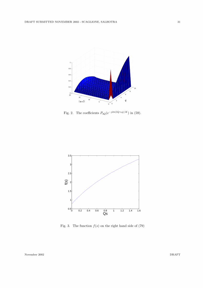
As can be noted from Fig.2 under (a3.), with the choice of p = (0, Q, . . . , QL) the coef-
ficients of the linear combination in (54) that corresponds to H [lQ + q] are for the most
November 2002 DRAFT

DRAFT SUBMITTED NOVEMBER 2002 - SCAGLIONE, SALHOTRA 18
part highly concentrated around l − n = 0, which suggest the approximation:
H [lQ + q] ≈ PlQ(e−j2π(lQ+q)/K)H [lQ] = α(q)H [lQ]. (60)
where
α(q) , ej2π( qLQ(L+1))
L + 1
sin(
)
sin(
πqQ(L+1)
) (61)
In addition, let us assume that:
a4. In assumption a2. RH(l1, l2) = RH(l2 − l1).
In general, this condition rarely applies because, for example, the paths are likely not to
have the same average power. However, this assumption describes a worse case scenario
in terms of the frequency selectivity of the channel and helps simplifying the derivations
considerably. In fact, if p is selected to have uniformly spaced frequency indices, in
force of Szego theorem for L À 1 the elements of H [p] will be approximately uncorre-
lated not only in space, but also across the frequency bins. Since the correlation matrix
of H(d) is (I ⊗ RH), using the central limit theorem the p.d.f. of H [p] is approxi-
mately5 v N (0 ,(W HL+1(p)RHW L+1(p) ⊗ I)) where (W H
L+1RHW L+1) ≈ diag(σ2h[p])
where σ2h[p] = (σ2
h[0], .., σ2h[LQ]) and σ2
h[lQ] =∑
n RH [n]e−j2πnl/(L+1). This leads to the
following:
Proposition 2: Under a1, a3, a4 for L À 1 and assuming EH [p] = 0 the HH
[lQ]
are approximately Gaussian and independent and
Φc(s) ≈ χ3
L∏
l=0
∫ Q−1∏q=0
∣∣∣I + γα(q)HH
[lQ]H [lQ]∣∣∣s
e− tr(H
H[lQ]H[lQ])
σ2h[l] (dH [lQ]), (62)
where χ3 =∏L
l=0(πσ2h[l])
NT NR = πNT NR(L+1)|RH |NT NR . The closed form expression of the
integral on the right side of (62) is analogous to (44) [18], [19].
Because (44) is not intelligible anyways, we prefer to proceed in our approximation and
exploit the fact that γ À 1. In this case is also easier to consider spatial correlation when
it is reasonable to assume that the correlation does not change with the path and the
following separable model applies:
EH [l]∗r1,t1H [l]r2,t2 = Rrr1,r2Rtt1,t2 . (63)
5Under (a2) this is obviously exactly true.
November 2002 DRAFT

DRAFT SUBMITTED NOVEMBER 2002 - SCAGLIONE, SALHOTRA 19
Overall this means that the covariance matrix of H [d] is Rr ⊗Rt ⊗RH . Since the DFT
operates in time, the spatial correlation of the MIMO frequency response H [p] for L À 1
tend to be Rr ⊗Rt ⊗ diag(σ2h[p]), or in other words
E[vec(H [lQ])vec(H [lQ])H ] = σ2[lQ](Rt ⊗Rr). (64)
With this in mind we can state the following
Proposition 3: Under the same assumptions and using the same approximations that
lead to Proposition 2, if γ À 1:
ΦC(s) ≈ |Rt|sK |Rr|sK(γ|RH |
1L+1
)sKn(
Q−1∏q=0
α(q)
)s(L+1)n (n∏
i=1
Γ(Qs + m− n + i)
Γ(m− n + i)
)L+1
(65)
Proof: When γ À 1 the contribution of the identity matrix to the determinant in
(62) can be neglected leading to:
ΦC(s) ≈L∏
l=0
E
Q−1∏q=0
|γα(q)HH
[lQ]H [lQ]|s
=L∏
l=0
E
Q−1∏q=0
|γα(q)R1/2t R
−1/2t H
H[lQ]R−1/2
r RrR−1/2r H [lQ]R
−1/2t R
1/2t |s
= γKsn|Rt|Ks|Rr|Ks
(L∏
l=0
σ2[lQ]
)Qsn (Q−1∏q=0
α(q)
)sn(L+1)
· E|R−1/2
r H [lQ]R−1/2t /σ[lQ]|2Qs
= γKsn|Rt|Ks|Rr|Ks|RH |Qsn
(Q−1∏q=0
αsn(L+1)(q)
)E
|W |2Qs
(66)
where E|W |2Qs
is the expectation of the random determinant of a complex Gaussian
zero mean matrix with independent entries having unit variance. The expression of the
expectation is:
E|W |2Qs
= E
n∏
i=1
λQsi
=
∫
λ≥0
(n∏
i=1
λQsi
)pΛ(λ1 · · ·λn)(dΛ)
=
∫
λ≥0
(n∏
i=1
λQsi
)χ
∏
1≤i<k≤n
(λk − λi)2e−
∑i λi
(n∏
i=1
λi
)m−n
(dΛ)
November 2002 DRAFT

DRAFT SUBMITTED NOVEMBER 2002 - SCAGLIONE, SALHOTRA 20
where χ is given by (c.f. (17), (18) for V ol(Qm,n) V ol(Un,n))
χ = 2−nπ−mn V ol(Qm,n) V ol(Un,n) =1∏n
i=1 Γ(i)Γ(m− n + i). (67)
Because:n∏
i=1
Γ(i)Γ(α + i) =
∫
λi≥0
(n∏
i=1
λi
)α
e−∑
i λi
n∏
1≤i<k≤n
(λk − λi)2(dΛ), (68)
from (68) we have
E
n∏
i=1
λQsi
= χ
n∏i=1
Γ(i)Γ(Qs + m− n + i), (69)
and this leads to (65).
A. The Gaussian approximation
As pointed out earlier in this section, the Capacity for the case of γ ¿ 1 takes the
following form
C ≈ γKtr(HH [d]H [d]) (70)
This is a χ− square distribution which, under the limit of large number of antennas and
paths, will closely approximate the Gaussian density. However, even for the reasonable
values of NR and NT , we show that the Gaussian fit is accurate even when γ is really
small. To do so, we first find parameters of the corresponding Gaussian random variable
using (49). First and second order derivatives of ΦC(s) evaluated at s = 0 yield the mean
and variance 6 :
µ = γKtr(Rr)tr(Rt)tr(RH), σ2 = (γK)2tr(R2r)tr(R
2t )tr(R
2H) (71)
Hence, we have, in this case, the following
pC(C) ≈ e− (C−γKtr(R))2
2(γK)2tr(R2)
√2π(γK)2tr(R
2)
. (72)
It is interesting to note that mean and variance are proportional to the signal to noise
ratio (γ). Also, while there is no explicit dependence on m and n, the dependence on the
6We use the identity ∂∂αln |A| = tr
A−1 ∂A
∂α
November 2002 DRAFT

DRAFT SUBMITTED NOVEMBER 2002 - SCAGLIONE, SALHOTRA 21
correlation matrices of paths and the array elements is through their trace. The Gaussian
approximation is compared with the Capacity histogram in Fig.6 (See section VIII for
details). It is interesting to observe that the mean normalized by the standard deviation
is 1. As we shall see later, the dependence of γ, RH , Rt, Rr, m and n on the mean and
variance is entirely different when we consider γ to be high.
In fact, for high γ, (65) shows that the channel gain takes the form of the geometric
mean of the eigenvalues of the channel covariance matrix. The form of the characteristic
function in (65) motivates the idea of approximating the p.d.f. of Capacity with a Gaussian
p.d.f. whose parameters can be easily computed. From (65),
ΦC(s) =
Q−1∏q=0
(α(q)γ|RH |1
L+1 |Rt|1/n|Rr|1/n)sn(L+1)
(n∏
i=1
Γ(Qs + m− n + i)
Γ(m− n + i)
)L+1
= esn(L+1) log
(∏Q−1q=0
(α(q)γ|RH |
1L+1 |Rt|1/n|Rr|1/n
)) (n∏
i=1
Γ(Qs + m− n + i)
Γ(m− n + i)
)L+1
(73)
The first factor in (73) implies that the Capacity p.d.f. pC(C) is a shifted version of the
inverse Laplace transform of the term
(n∏
i=1
Γ(Qs + m− n + i)
Γ(m− n + i)
)L+1
. (74)
The factor (74) is the Lth power of a product of functions. Since in our approximations
L À 1, we can infer that the inverse Laplace transform of (74) will be very close to a
Gaussian p.d.f., using the same arguments used in the proof of the central limit theorem.
Even when L is moderately large, the product inside indicates that several convolutions
take place in the inverse domain, so that the same conclusion holds approximately true.
From the first and second order derivatives of Γ(Qs+m−n+i)Γ(m−n+i)
in s = 0, one can easily obtain
the first order moment µ(1)i and the variance σ2
i of its inverse Laplace transform, which
are:
µi = Qψ(0)(m− n + i) , σ2i = Q2ψ(2)(m− n + i), (75)
where ψn(x) is the nth derivative of the Polygamma function also known as Digamma
function [20]. Therefore, shifting by(∏Q−1
q=0 α(q)γ|RH |1
L+1 |Rt| 1n |Rr| 1n)
the inverse Laplace
November 2002 DRAFT

DRAFT SUBMITTED NOVEMBER 2002 - SCAGLIONE, SALHOTRA 22
transform of
[(Γ(Qs+m−n+i)
Γ(m−n+i)
)L+1], we have that approximately:
pC(C) ≈ e−
(C−
(∏Q−1
q=0 α(q)γ|RH |1
L+1 |Rt|1/n|Rr |1/n
)−K
∑ni=1 ψ(0)(m−n+i)
)2
2KQ∑n
i=1ψ(2)(m−n+i)
√2πKQ
∑ni=1 ψ(2)(m− n + i)
. (76)
It should be noted that the variance of the Capacity (75) obtained in the high SNR regime
is independent of γ and the same conclusion was reached in [21]. This is in direct contrast
to the low γ scenario. Here we also notice that, even if under many approximations, the
effect of correlation and SNR is only to shift the mean of the distribution but the same
parameters have no impact on the Capacity variance, which is only a function of m,n. The
peculiar dependence on the correlation of paths and array elements through the geometric
mean of the eigenvalues is also quite interesting and provides further confirmation of
the fact that antenna elements and multi-path have similar effects on the Capacity in
broadband channels.
In the section (VIII), we present the plots of characteristic function given by (65) for a
frequency selective channel for different values of Q . We also provide the corresponding
plots, using Monte Carlo simulation, of (39) and show that both the expressions for char-
acteristic function are same when number of frequency bins equals the channel duration,
i.e. when Q = 1 .
VII. Outage Capacity and Chernoff Bound
We consider the case of γ À 1 only. The case of low γ requires calculating the cumula-
tive distribution function of a χ − square density and the comparison with its Gaussian
approximation is available in literature [22] and will not be considered here for brevity.
With the characteristic function and the Gaussian approximation (76) of the p.d.f for high
γ case at hand, it is possible to derive curves that come close to the Outage Capacity.
Using the Chernoff bound:
Pr(C > V ) ≤ mins≥0e−sV +log EesC (77)
November 2002 DRAFT

DRAFT SUBMITTED NOVEMBER 2002 - SCAGLIONE, SALHOTRA 23
To find the tightest bound we equate to zero the derivative of −sV + log EesC with
respect to s and obtain the following equivalent equation:
⇒ V = n(L + 1) log
(Q−1∏q=0
α(q)γ|RH |1
L+1 |Rt|1/n|Rr|1/n
)+
(L + 1)n∑
i=1
d
dslog(Γ(Qs + m− n + i)) (78)
Let ρ , V − n(L + 1) log(∏Q−1
q=0 α(q)γ|RH |1
L+1 |Rt|1/n|Rr|1/n)
, then from (78)
ρ = (L + 1)n∑
i=1
d
dslog(Γ(Qs + m− n + i)) = K
n∑i=1
ψ(0)(Qs + m− n + i). (79)
The expression on the right hand side of (79), say f(s), is a monotonic function of Qs (see
Fig.3)
The intersection of this monotonic function f(s) with horizontal family of curves for
different values of V gives the optimum value of s that minimizes (77) [c.f. Section VIII].
With the Gaussian approximation derived in Section VI-A, the Outage Capacity is
simply
Pr(C > V ) = Q
V −
(∏Q−1q=0 α(q)γ|RH |
1L+1 |Rt|1/n|Rr|1/n
)−K
∑ni=1 ψ(0)(m− n + i)
√KQ
∑ni=1 ψ(2)(m− n + i)
(80)
where Q(x) is the Q-function and ψ(n)(x) is, as mentioned before, the nth derivative of
the Polygamma function also known as Digamma function.
VIII. Numerical Examples
In this section we conclude our work by presenting some numerical examples supporting
the theoretical results obtained in the paper. We first present plots of the characteristic
function for different channel parameters. The characteristic function given by (65) is
plotted and compared with the the characteristic function obtained by Monte Carlo sim-
ulations (39). In all examples, the number of frequency bins is K = 8 and the signal to
noise ratio (γ) of the channel is assumed to be 20dB. In (Fig.4), the characteristic func-
tions from (65) and (39) for various values of L are plotted together. We obtained these
November 2002 DRAFT

DRAFT SUBMITTED NOVEMBER 2002 - SCAGLIONE, SALHOTRA 24
curves for NR = 3, NT = 4 for the case where the paths and array elements correlations
are homogeneous and decay exponentially, i.e. RH(l2, l1) = ρ|l2−l1|, Rt(t2, t1) = ρ|t2−t1|
and Rr(r2, r1) = ρ|r2−r1| respectively, with ρ = 0.5. We can see that as L increases, the
approximate expression (the solid curve) closes towards the exact one, and the approxi-
mation becomes exact when the number of frequency bins equals the channel duration,
i.e. when Q = 1 . This is shown by the pair of curves for K = 8, L = 7.
Fig.5 shows the effect of the signal to noise ratio (γ) on the accuracy of the approximate
expression in (65). In this example K = 8, L = 7, NR = 3, NT = 4 and the correlations
in time and space are identical to the ones used in the previous example. Since we arrived
at (65) under high SNR assumption, we can expect intuitively the approximation to be
better at high γ. This is evident from the (Fig.5), where we observe that the plots merge
as γ is increased from 5dB to 20dB.
The probability density function of the Capacity is plotted (see Fig.6) using Monte Carlo
simulations and compared with the one obtained by Gaussian density (72) when γ is very
small. The Gaussian approximation is really good and supports the claim made in the
section VI-A. Here, we have used K = 4, L = 3, ρ = 0.1, NR = 6, NT = 6 and γ = -35
dB. The normalized histogram of Capacity for high γ is also shown in (Fig.7) and it is
in a very good agreement with (73), which appears to be accurate even for low values of
the Outage Capacity. K = 8, L = 7, ρ = 0.3, NR = 3, NT = 3 and γ = 35 dB are used.
Hence, the Gaussian approximation works fine for low as well as high signal to noise ratio
even for moderate values of NR and NT , as observed by other authors [21], [23].
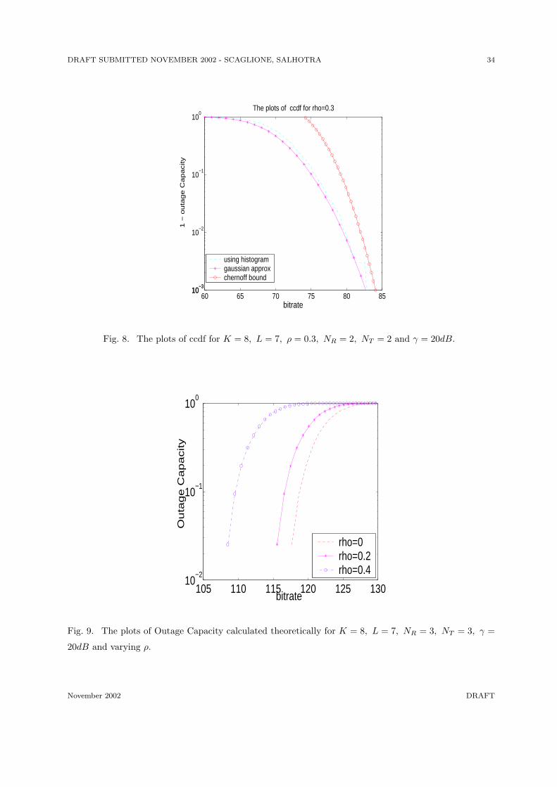
In Fig.8 we show the Chernoff bound for the Capacity, the complementary cumu-
lative distribution function (ccdf) of Capacity using (80) and compare them with the
corresponding values obtained by Monte Carlo simulations. The parameters used are
K = 8, L = 7, ρ = 0.3, NR = 2, NT = 2 and γ = 20 dB. The effect of correlated fading
is illustrated in (Fig.9) using the same exponential model for path and array correlation
described above and changing the value of ρ. We consider ρ = 0 (uncorrelated case),
ρ = 0.2 and ρ = 0.4. and, as before, the parameters are K = 8, L = 7, NR = 3, NT = 3
and γ = 20dB. It is interesting to observe that the outage Capacity increases as ρ in-
creases. In fact, the correlation between the antenna elements reduces the diversity and
November 2002 DRAFT

DRAFT SUBMITTED NOVEMBER 2002 - SCAGLIONE, SALHOTRA 25
hence increases the outage.
Appendix
A. The computation of (dB) where B = QR and the volume element of a unitary group
Since we could not find the derivation of (16) anywhere, we thought of adding this
appendix. The Householder reflections can be used to decompose any matrix, A ∈ Cm,n
(m ≥ n) as a product of a unitary and an upper triangular matrix. The complex House-
holder reflection is given by
H = I − 2vvH
vHv, (81)
and it is easy to verify that H is Hermitian and unitary. Similar to the what is done for
the real case in [13], we can write:
HnHn−1 · · ·H1A =
Rn×n
0
⇒ A = H1H2 · · ·Hn
Rn×n
0
, (82)
where Q = H1H2 · · ·Hn is the product of the Householder reflections. From (82), we
can write A = QR, where Q includes only the first n columns of H1H2 · · ·Hn (i.e.
Q = [q1 · · · qn]).
A has 2mn real parameters and, therefore, the total number of independent parameters
of R and Q needs to be 2mn for A = QR to be a unique transformation. Q satisfies
QHQ = I, which corresponds to n + 2n(n−1)2
= n2 equations. Hence, the Stiefel manifold
has 2mn − n2 real independent parameters. R has n(n + 1)/2 complex parameters and
twice as many real, which is n too many. Hence in order to have unique factorization in
(82), we can constrain the diagonal elements of R to be real so that R has n2 independent
parameters only. Now, we can proceed to calculate (dA) = (QH
dA).
(QH
dA) = (QH
QdR + QH
dQR)
= (Im,ndR + QH
dQR). (83)
The first term is an m × n upper triangular matrix while QH
dQ is antisymmetric with
purely imaginary diagonal elements7. In fact, qHi qi = 1 implies qH
i dqi = −dqHi qi =
−(qHi dqi)
∗ and then <(qHi dqi) = 0. Also, qH
i dqj = −(qHj dqi)
∗.
7The presence of these imaginary diagonal entries makes the case of unitary and orthogonal case different.
November 2002 DRAFT
DRAFT SUBMITTED NOVEMBER 2002 - SCAGLIONE, SALHOTRA 26
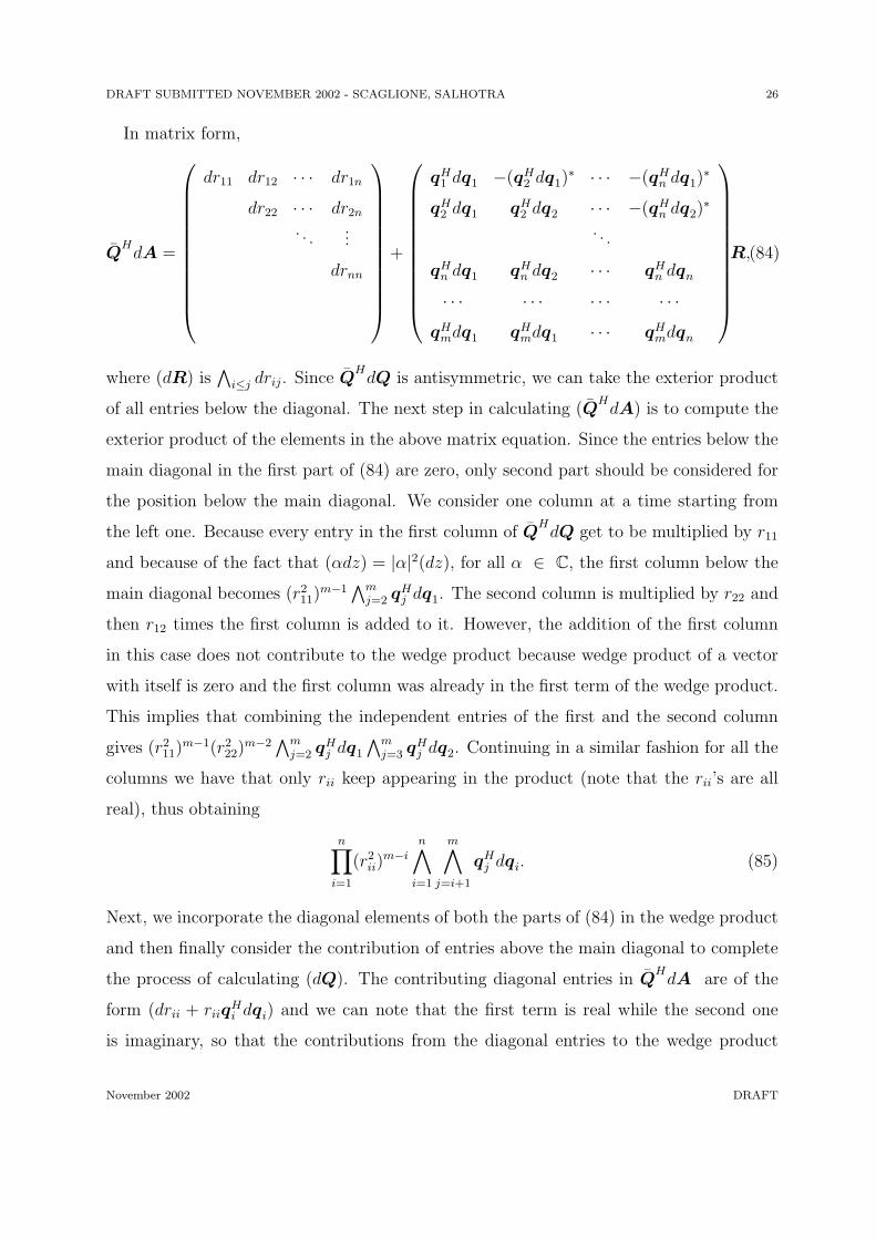
In matrix form,
QH
dA =
dr11 dr12 · · · dr1n
dr22 · · · dr2n
. . ....
drnn
+
qH1 dq1 −(qH
2 dq1)∗ · · · −(qH
n dq1)∗
qH2 dq1 qH
2 dq2 · · · −(qHn dq2)
∗
. . .
qHn dq1 qH
n dq2 · · · qHn dqn
· · · · · · · · · · · ·qH
mdq1 qHmdq1 · · · qH
mdqn
R,(84)
where (dR) is∧
i≤j drij. Since QH
dQ is antisymmetric, we can take the exterior product
of all entries below the diagonal. The next step in calculating (QH
dA) is to compute the
exterior product of the elements in the above matrix equation. Since the entries below the
main diagonal in the first part of (84) are zero, only second part should be considered for
the position below the main diagonal. We consider one column at a time starting from
the left one. Because every entry in the first column of QH
dQ get to be multiplied by r11
and because of the fact that (αdz) = |α|2(dz), for all α ∈ C, the first column below the
main diagonal becomes (r211)
m−1∧m
j=2 qHj dq1. The second column is multiplied by r22 and
then r12 times the first column is added to it. However, the addition of the first column
in this case does not contribute to the wedge product because wedge product of a vector
with itself is zero and the first column was already in the first term of the wedge product.
This implies that combining the independent entries of the first and the second column
gives (r211)
m−1(r222)
m−2∧m
j=2 qHj dq1
∧mj=3 qH
j dq2. Continuing in a similar fashion for all the
columns we have that only rii keep appearing in the product (note that the rii’s are all
real), thus obtaining
n∏i=1
(r2ii)
m−i
n∧i=1
m∧j=i+1
qHj dqi. (85)
Next, we incorporate the diagonal elements of both the parts of (84) in the wedge product
and then finally consider the contribution of entries above the main diagonal to complete
the process of calculating (dQ). The contributing diagonal entries in QH
dA are of the
form (drii + riiqHi dqi) and we can note that the first term is real while the second one
is imaginary, so that the contributions from the diagonal entries to the wedge product
November 2002 DRAFT
DRAFT SUBMITTED NOVEMBER 2002 - SCAGLIONE, SALHOTRA 27
appear as
n∏i=1
(rii)(dr11 ∧ dr22 · · · ∧ drnn)(qH1 dq1 ∧ · · · ∧ qH
n dqn). (86)
For the entries above the main diagonal, only the first part in (84) contributes to the
wedge product (because of the fact that dz ∧ dz∗ = 0) taking the form
∧i<j
drij. (87)
Equations (85), (86) and (87) can now be combined to produce (QH
dA) = (dA) as
(QH
dA) =n∏
i=1
(rii)2(m−i)+1
n∧i=1
m∧j=i
qHj dqi
∧i≤j
drij
=n∏
i=1
(rii)2(m−i)+1
n∧i=1
m∧j=i
qHj dqi(dR). (88)
Writing∧n
i=1
∧mj=i q
Hj dqi in the above equation as (dQ), (dA) can finally be written as
(dA) =n∏
i=1
(rii)2(m−i)+1(dQ)(dR) (89)
The element of volume of Stiefel manifold is thus simply
(dQ) =n∧
i=1
m∧j=i
qHj dqi, (90)
where, noticeably the elements for j = i have to be included, contrary to the case of
orthogonal matrices Q ∈ Rm,n , QT Q = I for which:
(dQ) =n∧
i=1
m∧j=i+1
qTj dqi. (91)
As an example, we give the volume element of a 2 × 2 unitary group for the following
parametrization [24]
Q(ξ1, ξ2, ξ3, ξ4) =
cos ξ1e
− ξ2 sin ξ1e− ξ3
− sin ξ1e ξ3 cos ξ1e
ξ2
e ξ4 (92)
The element of volume for such a group can be calculated(using (90))to be
(dQ) = 2| sin ξ1 cos ξ1| d(ξ1, ξ2, ξ3, ξ4), 0 ≤ ξ1, ξ2, ξ3, ξ4 < 2π (93)
November 2002 DRAFT
DRAFT SUBMITTED NOVEMBER 2002 - SCAGLIONE, SALHOTRA 28
References
[1] E. Telatar, “Capacity of multi-antenna Gaussian channels, Tech. Rep. Bell Laboratories, 1995.
[2] G.J. Foschini, “Layered space-time architecture for wireless communication in a fading environment when using
multielement antennas,” Bell Labs. Tech. Journ., Vol. 1, No. 2, pp. 41–59, 1996.
[3] T.L. Marzetta, B. H. Hochwald, “Capacity of a mobile multiple-antenna communication link in Rayleigh flat
fading”, IEEE Trans. on Info. Theory, Vol. 45, No. 1, pp.139-157, Jan. 1999.
[4] Alex Grant, “Rayleigh Fading Multi-Antenna Channels,” EURASIP Journal on Applied Signal processing,
Vol.2002,Issue 3 pp. 316–329.
[5] Lizhong Zheng, David N.C. Tse, “Communication on the Grassmann Manifold: A Geometric Approach to the
Noncoherent Multiple-Antenna Channel”, IEEE Trans. on Info. Theory, Vol. 48, No. 2, pp.359-383, Feb. 2002.
[6] P. B. Rapajic and D. Popescu, “Information Capacity of a Random Signature Multiple-Input Multiple-Output
Channel,” IEEE Trans. on Commun., Vol. 48, No. 8, pp. 1245–1248, August 2000.
[7] Y.Li, J. Chuang, N. R. Sollenberger, “Transmitter diversity for ofdm systems and its impacts on high-rate
wireless networks,” Proc. of IEEE Int. Conf. on Comm., Vol. 1, pp. 534–538, Vancouver, Canada, June 1999.
[8] M.K Simon, M.S. Alouini “Digital Communication over Fading Channels, A Unified approach to Performance
Analysis”, Wiley Interscience, 2000.
[9] E. Wigner, “On the distribution of the roots of certain symmetric matrices,” Annales of Math. Vol. 67, pp.325–
327, 1958.
[10] A. Edelman, “Random Eigenvalues,” Notes for Math 273 UC Berkeley, Feb. 27, 1999
http://www.math.berkeley.edu/ edelman/math273.html
[11] V. Girko, “Theory of Random Determinants” Kluwer Publishers(Netherlands) 1990.
[12] H. Flandes, “Diffrential Forms with Applications to teh Physical Sciences”, Dover Publications Inc., New
York, II Edition, 1989.
[13] G. H. Golub, C. F. Van Loan, “Matrix Computations”, The Johns Hopkins University Press, III Edition,1996.
[14] A.T. James, “Distributions of matrix variates and laltent roots derived from normal samples,” Ann. Math.
Statistics, Vol. 35, pp.475-501, 1964.
[15] Haagerup and S. Thorbjrnsen, “Random matrices with complex Gaussian entries,” preprint (49 pp.), Odense
1998. http://www.imada.ou.dk/ haagerup/2000-.html.
[16] B.V. Bronk, “Exponential ensembles for Random matrices”, Jour. of Math. Physics, Vol. 6, pp. 228-237,
1965.
[17] A. Lozano, A. Tulino and S. Verdu, “Multi-Antenna Capacity in the Low-power Regime”, DIMACS Workshop
on Signal Processing for Wireless Transmission, Rutgers,October 2002.
[18] M. Kang and M. -S. Alouini, “Quadratic forms in complex Gaussian matrices and performance analysis
of MIMO systems with co-channel interference”,Proceedings of IEEE International on Information Theory
(ISIT’2002), p. , Lausanne, Switzerland, June 2002.
[19] Z. Wang and G. B. Giannakis, “Outage mutual information of space-time MIMO channels”, In Proc. of 40th
Allerton Conf,October 2002.
[20] E. Artin, “The Gamma Function,” New York, Holt, Rinehart and Winston, 1964.
[21] T.L. Marzetta, B. M. Hochwald and V. Tarokh“Multi-Antenna Channel-Hardening and its Implications
for Rate Feedback and Scheduling” Submitted to IEEE Transactions on Information Theory, May 2002.
preprinthttp://mars.bell-labs.com/cm/ms/what/mars/papers/ratefeedback/
[22] Steven M. Kay, “Fundamentals of Statistical Signal Processing- Detection Theory”, Prentice Hall, 1998.
November 2002 DRAFT

DRAFT SUBMITTED NOVEMBER 2002 - SCAGLIONE, SALHOTRA 29
[23] P.J. Smith and M. Shafi, “On a Gaussian Approximation to the Capacity of Wireless MIMO Systems”, IEEE
International Conference on Communications(ICC),New York city,April-May 2002.
[24] F. D. Murnaghan, “The Theory of Group Representations”, The John Hopkins Press, Baltimore, 1938.
November 2002 DRAFT
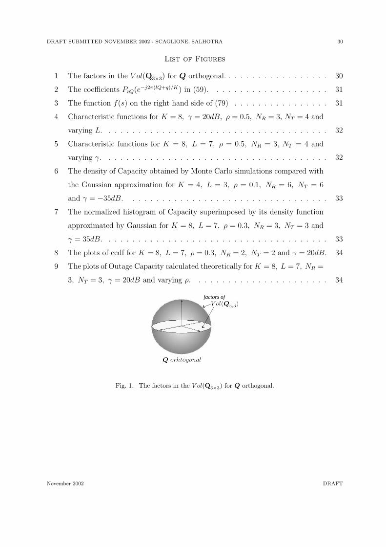
DRAFT SUBMITTED NOVEMBER 2002 - SCAGLIONE, SALHOTRA 30
List of Figures
1 The factors in the V ol(Q3×3) for Q orthogonal. . . . . . . . . . . . . . . . . . 30
2 The coefficients PnQ(e−j2π(lQ+q)/K) in (59). . . . . . . . . . . . . . . . . . . . 31
3 The function f(s) on the right hand side of (79) . . . . . . . . . . . . . . . . 31
4 Characteristic functions for K = 8, γ = 20dB, ρ = 0.5, NR = 3, NT = 4 and
varying L. . . . . . . . . . . . . . . . . . . . . . . . . . . . . . . . . . . . . . 32
5 Characteristic functions for K = 8, L = 7, ρ = 0.5, NR = 3, NT = 4 and
varying γ. . . . . . . . . . . . . . . . . . . . . . . . . . . . . . . . . . . . . . 32
6 The density of Capacity obtained by Monte Carlo simulations compared with
the Gaussian approximation for K = 4, L = 3, ρ = 0.1, NR = 6, NT = 6
and γ = −35dB. . . . . . . . . . . . . . . . . . . . . . . . . . . . . . . . . . 33
7 The normalized histogram of Capacity superimposed by its density function
approximated by Gaussian for K = 8, L = 7, ρ = 0.3, NR = 3, NT = 3 and
γ = 35dB. . . . . . . . . . . . . . . . . . . . . . . . . . . . . . . . . . . . . . 33
8 The plots of ccdf for K = 8, L = 7, ρ = 0.3, NR = 2, NT = 2 and γ = 20dB. 34
9 The plots of Outage Capacity calculated theoretically for K = 8, L = 7, NR =
3, NT = 3, γ = 20dB and varying ρ. . . . . . . . . . . . . . . . . . . . . . . 34
factors of
Fig. 1. The factors in the V ol(Q3×3) for Q orthogonal.
November 2002 DRAFT
DRAFT SUBMITTED NOVEMBER 2002 - SCAGLIONE, SALHOTRA 31
0
2
4
6
8
10
05
1015
200
0.2
0.4
0.6
0.8
1
q|n−l|
Fig. 2. The coefficients PnQ(e−j2π(lQ+q)/K) in (59).
0 0.2 0.4 0.6 0.8 1 1.2 1.4 1.60.5
1
1.5
2
2.5
3
3.5
Qs
f(s)
Fig. 3. The function f(s) on the right hand side of (79)
November 2002 DRAFT

DRAFT SUBMITTED NOVEMBER 2002 - SCAGLIONE, SALHOTRA 32
0 0.25 0.5 0.75 1 1.2510
−40
10−20
100
1020
1040
1060 Characteristic function of C for K=8,snr=20dB
S
phiC
(S)
K=8,L=2
K=8,L=7
K=8,L=5
Using approximations Using Monte Carlo sim
Fig. 4. Characteristic functions for K = 8, γ = 20dB, ρ = 0.5, NR = 3, NT = 4 and varying L.
0 0.25 0.5 0.75 1 1.25
10−20
10−10
100
1010
1020
1030
1040
Characteristic function of C for K=8,L=7, different snr
S
ph
iC(S
)
snr= 5dB
Using approximations Using Monte Carlo sim
snr= 15dB
snr= 20dB
Fig. 5. Characteristic functions for K = 8, L = 7, ρ = 0.5, NR = 3, NT = 4 and varying γ.
November 2002 DRAFT

DRAFT SUBMITTED NOVEMBER 2002 - SCAGLIONE, SALHOTRA 33
0.1 0.15 0.2 0.250
5
10
15
20
25
30
Capacity
histogram of Capacitygaussian approximation
snr= −35dB
Fig. 6. The density of Capacity obtained by Monte Carlo simulations compared with the Gaussian
approximation for K = 4, L = 3, ρ = 0.1, NR = 6, NT = 6 and γ = −35dB.
170 180 190 200 210 2200
0.02
0.04
0.06
0.08
0.1
Capacity
histogram of Capacitygaussian approximation
snr = 35dB
Fig. 7. The normalized histogram of Capacity superimposed by its density function approximated by
Gaussian for K = 8, L = 7, ρ = 0.3, NR = 3, NT = 3 and γ = 35dB.
November 2002 DRAFT
DRAFT SUBMITTED NOVEMBER 2002 - SCAGLIONE, SALHOTRA 34
60 65 70 75 80 8510
−310
−3
10−2
10−1
100
The plots of ccdf for rho=0.3
1 −
ou
tag
e C
ap
acity
using histogramgaussian approxchernoff bound
bitrate
Fig. 8. The plots of ccdf for K = 8, L = 7, ρ = 0.3, NR = 2, NT = 2 and γ = 20dB.
105 110 115 120 125 13010
−2
10−1
100
bitrate
Ou
tag
e C
ap
acity
rho=0rho=0.2rho=0.4
Fig. 9. The plots of Outage Capacity calculated theoretically for K = 8, L = 7, NR = 3, NT = 3, γ =
20dB and varying ρ.
November 2002 DRAFT