the statistical strength of forensic identi cation through

The statistical strength of forensic

identification through mobile phone

call data records

Helena B.R. van Eijk

Master thesis Mathematics (public version)Specialisation: Statistical Science for

Life and Behavioural Sciences

30 August 2013Thesis advisor: Prof. dr. R.D. Gill

Mathematisch Instituut, Universiteit Leiden

1

Contents

1 Introduction 41.1 Statistics in court . . . . . . . . . . . . . . . . . . . . . . . . . 51.2 Judicial miscarriages . . . . . . . . . . . . . . . . . . . . . . . 6

1.2.1 Sally Clark . . . . . . . . . . . . . . . . . . . . . . . . 71.2.2 Lucia de B. . . . . . . . . . . . . . . . . . . . . . . . . 7

1.3 Applicability . . . . . . . . . . . . . . . . . . . . . . . . . . . . 81.4 Cell Site Analysis . . . . . . . . . . . . . . . . . . . . . . . . . 91.5 Terminology . . . . . . . . . . . . . . . . . . . . . . . . . . . . 91.6 Aim of the research . . . . . . . . . . . . . . . . . . . . . . . . 10

1.6.1 Discovering colocating phones . . . . . . . . . . . . . . 101.6.2 Evaluating colocating phones . . . . . . . . . . . . . . 11

2 Discovering colocating phones 122.1 Proposed study design . . . . . . . . . . . . . . . . . . . . . . 122.2 Methods . . . . . . . . . . . . . . . . . . . . . . . . . . . . . . 132.3 Stratification . . . . . . . . . . . . . . . . . . . . . . . . . . . 142.4 Example data . . . . . . . . . . . . . . . . . . . . . . . . . . . 142.5 Conclusion . . . . . . . . . . . . . . . . . . . . . . . . . . . . . 152.6 Discussion . . . . . . . . . . . . . . . . . . . . . . . . . . . . . 16

2.6.1 Tunnel vision . . . . . . . . . . . . . . . . . . . . . . . 162.6.2 Unlikely events are not impossible . . . . . . . . . . . . 162.6.3 Large dataset . . . . . . . . . . . . . . . . . . . . . . . 17

3 Evaluating colocating phones 183.1 Texas sharpshooter . . . . . . . . . . . . . . . . . . . . . . . . 183.2 Aim . . . . . . . . . . . . . . . . . . . . . . . . . . . . . . . . 193.3 Visualisation . . . . . . . . . . . . . . . . . . . . . . . . . . . . 193.4 Data simulation . . . . . . . . . . . . . . . . . . . . . . . . . . 213.5 Methodology . . . . . . . . . . . . . . . . . . . . . . . . . . . 24

3.5.1 Permutation tests . . . . . . . . . . . . . . . . . . . . . 243.5.2 Measuring closeness . . . . . . . . . . . . . . . . . . . . 25

3.6 Results . . . . . . . . . . . . . . . . . . . . . . . . . . . . . . . 263.7 Reflection on the methodology and an adjustment . . . . . . . 30

3.7.1 Adjusting shuffling . . . . . . . . . . . . . . . . . . . . 303.7.2 Method . . . . . . . . . . . . . . . . . . . . . . . . . . 313.7.3 Results . . . . . . . . . . . . . . . . . . . . . . . . . . . 32

3.8 Validation method . . . . . . . . . . . . . . . . . . . . . . . . 323.9 Conclusion . . . . . . . . . . . . . . . . . . . . . . . . . . . . . 353.10 Discussion . . . . . . . . . . . . . . . . . . . . . . . . . . . . . 38

2

3.10.1 Reflection on the methodology . . . . . . . . . . . . . . 383.10.2 Relationship to other identification methods in forensic

science . . . . . . . . . . . . . . . . . . . . . . . . . . . 403.10.3 Relevant research . . . . . . . . . . . . . . . . . . . . . 423.10.4 Relationship to Likelihood Ratio . . . . . . . . . . . . 433.10.5 Recommendations for further research . . . . . . . . . 43

References 45

3

1 Introduction

Statistical approaches to analysing evidence play a central role in the criminaljustice system in the 21st century. Credible approaches to statistical analysisand their implementation in the court of law are therefore powerful entitiesin everyday life. When applied appropriately, the mathematical modeling ofstatistics can uniquely enhance the justice system. When applied inappropri-ately, it can undermine the justice system entirely. In this thesis, a methodis developed that can be applied on data that is coming from mobile phonerecords, which can potentially assist law enforcement agencies in their crim-inal investigation. During the past two decades, the development of mobilephones has progressed incredibly fast. In 2012 it was reported that 75% ofthe world’s population has access to a mobile phone. The number of phonesubscriptions has increased from 1 billion in 2000 to 6 billion in 2012 [15].It has also been noted that often multiple phones are owned by one person,leading to the expectation that the number of mobile phones will surpassthe human population. One reason for owning multiple phones could be tocover up criminal activity. Some criminals use a second (anonymous) phonesolely to communicate about such criminal activity, in order to make them-selves harder to trace. This development forces police departments to findnew methods to detect perpetrators by investigating phone records. Whenit is known that a crime was committed at a certain time and place, phonerecords will show which mobile phones were active in the area at that par-ticular time. This could assist the authorities in finding the perpetrator orcould be used as supporting evidence. However, especially among criminals,phones are often not registered to a known person, but are bought anony-mously. By studying phone records, patterns can occasionally be detectedthat connect two phones to each other. When the activity of two or morephones coincides both in time and location, a plausible explanation is thatthe phones are owned by one person. When a connection can be made be-tween an anonymous phone and a registered phone, this can be of additionalvalue in a criminal investigation. Within this thesis, a method is developedto test a suspected connection between two phones, and the statistical valueof such evidence is examined in an imaginary case for which data is simu-lated. Furthermore, approaches for distilling the vast amount of availabledata into credible evidence are implemented and evaluated. This thesis aimsto build on the advances made in this exciting field and safeguard againstthe ever-present and sometimes catastrophic pitfalls that are encountered tothis day within the criminal justice system.

4

1.1 Statistics in court

Over the past decades, the use of mathematical formulas and/or probabili-ties in court has been subject to debate, and is still much discussed withinthe field of forensic statistics. In 1970, Finkelstein & Fairley reviewed thedecision of the Californian Supreme Court in the Collins case to reject theprosecutor’s attempt to link the defendant to a crime by applying the prod-uct rule to the probabilities of the relevant characteristics [8]. Multiplyingprobabilities to calculate a joined probability is only valid for independentevents, and the court correctly declined the prosecutor’s argument. The useof mathematics in the Collins case contributed to the discussion on whetherstatistics should be allowed to be introduced in the trial context in orderto give weight to identification evidence. Finkelstein & Fairley state thatfor certain cases, it can be useful to statistically render an expert’s opin-ion, in order to assess the significance of the data [8]. They further arguethat “it is appropriate to translate frequencies of such events into a probabil-ity statement by combining them with prior probabilities through the use ofBayes’ Theorem”. One must always be aware that jurors can be swayed by amathematical explanation of events. Subsequently, inappropriate statisticalreasoning could lead a jury to hand down a conviction that is disproportion-ate to the strength of the evidence that supports it. However, Finkelsteinand Fairley feel that mathematics correctly used can be valuable in the eval-uation of identification evidence [8]. Tribe (1971) did not share this pointof view, which led to an interesting discussion between Finkelstein & Fairleyand Tribe [13], [9], [14]. Tribe studies the possible dangers that arise from theuse of mathematics in the legal process and finds its alleged usefulness greatlyexaggerated. The benefits of allowing mathematics at trial cannot equipoisethe severe consequences of possible errors. Tribe concluded that the use ofa Bayesian approach, or any similar technique, would be more misleadingthan helpful and stated that the conjunction of mathematics and the trialprocess would be more dangerous than fruitful [13]. In reaction to Tribe’sattack on their proposal, Finkelstein & Fairley once more emphasize thatan expert statistician can assist jurors with the interpretation of statisticalevidence that is coming from other experts. Numbers and probabilities arealready present in court, since a fingerprint expert will for instance state thatthe print found at the crime scene matches the defendant’s print, and thatsuch prints occur with a frequency of one in a thousand in the population.The expert statistician can help interpret this number and assist on the issuewhether the trace is left by the defendant [9]. Finally, Tribe maintains itsopinion that the techniques proposed by Finkelstein and Fairley can easily bemisused. He cannot think of a reason why a statement of an expert statisti-

5

cian will help a juror any better to place the evidence in perspective than theone-in-a-thousand finding. Real-life situations are rarely so straightforwardthat a mathematical model can grasp all its subtleties [14].

Recently, the discussion on statistics in court has resurfaced due to a verdictin a criminal case in the United Kingdom. In 2010, the Court of Appeal ruledthat it is accepted to use a mathematical approach to calculate the matchprobability in DNA cases, based on the reliability of the statistical database[1]. For other areas, such as the identification of footwear marks, data onthe distribution and use on footwear is not sufficient to allow an expert toexpress an opinion based on the use of a mathematical formula. “Outside thefield of DNA (and possibly other areas where there is a firm statistical base),this court has made it clear that Bayes theorem and likelihood ratios shouldnot be used” [1]. Fenton & Neil (2012) reacted to this ruling by stating thata proper use of probalistic reasoning can potentially improve the efficiencyand quality of the criminal justice system. “It is irrational to assume thatsome forensic evidence is statistically sound, whereas other less establishedforensic evidence is not” [6]. Critics of the ruling further recognize flaws inthe current presentation of probalistic evidence, but nevertheless convey theirconcerns on the impact of the ruling for future evidence presented by expertwitnesses. Berger, Buckleton, Champod, Evett & Jackson (2011) state thefollowing: “the evaluation of evidence for a court of law is not just a matterof “using likelihood ratios” but one of working to a set of principles that arefounded on logic. To deny scientists the contemplation of the likelihood ratio- whether quantitative or qualitative - is to deny the central element of thislogical structure.” [3]. When the statistical value of a new kind of evidenceis evaluated, as presented in this thesis, it is good practice to be mindful ofcurrent discussions pertaining to the use of statistics in court.

1.2 Judicial miscarriages

When mathematics and probabilities are used for the purpose of a criminalcase, it is of utmost importance to take heed of fallacies that have led to mis-carriages of justice in the past. In the evaluation of legal evidence, ideally thecircumstances would be such that not only the expert witness, but also the(prosecuting and defence) lawyers and judges possess sufficient knowledge tounderstand the numbers presented in court. Unfortunately, over the past fewdecades, miscarriages of justice have still occurred due to the use of statisticsin court. Schneps & Colmez (2013) [11] discuss several criminal cases wherewrongly applied statistical methods or incorrect interpretations of the cal-culated probabilities played an important role in the final verdict. Mistakes

6

made in court can lead to the conviction of innocent people, with severe con-sequences for their lives. Two recent examples of judicial miscarriage due tothe use of statistics will be briefly discussed.

1.2.1 Sally Clark

In the United Kingdom, Sally Clark experienced the effect of wrongly cal-culated probabilities. The loss of her two baby boys by an unknown cause(also known as crib death) was considered as two independent events. The(low) probability of experiencing a crib death in her social class was squared,without taking into account that it is very likely that these two boys didnot die independently and that there was an underlying undetected geneticdisease or disorder. The outcome was disastrous as Sally Clark was depictedas a ruthless child murderer, spent years in prison, never recovered from thiswrongful accusation and died from an alcohol overdose four years after herrelease. For Sally, the event of losing a second child to an unknown causeshould have never been considered to be independent from the event of losinga first child. Nevertheless, this calculation was made, and the result has beentremendous [11].

1.2.2 Lucia de B.

In the Netherlands, the case of Lucia de B. is well known when it comes towrongfully applying probabilities in court. This dramatic course of eventsstarted when colleagues of this nurse noted that she was often present duringan unexpected death of a baby, causing her supervisor to come suspiciousthat her presence had something to do with the deaths. Data was collected onthe number of shifts with or without incident, with or without Lucia present,and a statistic was assigned to the probability that the incidents among herpatients had happened under her supervision by chance. From this data, aDutch psychologist (who was assigned as an expert witness) concluded thatthis combination of events would only occur by chance in about 1 of 9 mil-lion cases of a nurse working at a hospital for nine months. This numberwas multiplied with the probability calculated from similar statistics comingfrom the two other hospitals where Lucia worked, leading to a baffling num-ber of 1 in 342 million. Since this number is so small, the conclusion wasdrawn that it simply could not have occurred naturally. With help from themedia, Lucia was soon painted as a remorseless baby killer, and she foundherself suddenly accused of multiple murders and attempted murders. How-ever, after her conviction and a reopening of the case, it was demonstratedthat the numbers in the dataset that documented Lucia’s presence and the

7

occurrences of incidents were incorrect in the first place, and that the multi-plication of the probabilities should have never been done, since the eventscannot be considered independent. In 2010, Lucia de B. received the verdictof not guilty, after spending more than six years in prison [11].

The examples mentioned above show that even in the past decades, mis-understandings are still present when numbers and probabilities are usedin court. Both cases suffer from an inappropriately applied multiplication ofprobabilities of events that cannot be considered as independent occurrences.As mentioned previously, the statistical value of a particular type of evidencewill be addressed in this thesis. Mathematics is used and the probability thata certain event occurred by chance is central to this case. With the recentmiscarriages of justice in mind, the presented experiments will be related tothe current topics in the field of forensic statistics. Throughout the thesisit is elucidated which errors should be considered as having the potential torecur in future when a statistical value is assigned to legal evidence whichcan be presented in court.

1.3 Applicability

The method developed in this thesis can be applied to test the hypothesiswhether two phones are probable to be used by the same person. Whenphone records are available of two phones that show a similar pattern withrespect to the time and location of their calls, this method can be used totest the significance of this cohesion. Within the field of law enforcement,this can be of use in criminal cases where a phone is found to behave in asuspicious way around the time of the crime. If the phone is related to thecrime, it probably has no contract attached to it from which the identity ofthe suspect can be detected. It is possible that the perpetrator is using thisanonymous phone to prepare or execute the crime, and actively uses a second(registered) phone. It is easy to imagine that a criminal who is using a phonein the preparation of a criminal conduct, is carrying another phone to use forday-to-day and personal business. The phone records of these two phoneswill show similarity in the time and location of their calls. The methodpresented in this thesis aims to determine the significance of this observedconnection between phones, in order to potentially increase the reliabilityof presented evidence in court. A defence argument could be that a searchamong all phone records will yield a connection between phones by chanceand that this does not necessarily mean that phones are used by the sameperson. The current study will therefore discuss a method to quantify theevidential value of such evidence.

8

1.4 Cell Site Analysis

When the physical movements of a mobile phone are reconstructed, one entersthe field of Cell Site Analysis. Mobile telephone operators store call data thatcan be analysed to determine the location of a mobile phone at the time of acall, SMS or MMS. Analyses on these call data records can produce evidencethat can possibly be of use in a criminal investigation where a suspect’smovement is of interest. An alibi could be checked, movements of suspectscould be followed or the presence at a crime scene could be confirmed.

The method introduced in this thesis can contribute to the field of Cell SiteAnalysis when one wants to attribute a phone to an individual through theuse of Cell Site Analysis. When a phone has no contract attached to it, itis difficult to attribute an individual to it. When there is a phone withoutcontract of note in the investigation, the movements of this phone could becompared with attributed contract phones, to see if a connection can possiblybe detected between the anonymous phone and a contract phone. Dr. IainBrodie states that such analysis on “clean and dirty phones” is a commonmethod used in law enforcement [4]. Focussing on time and location, dr.Brodie looks for similar patterns of movements for the two phones and triesto find a sufficient amount of similarities in order to show beyond reasonabledoubt that two phones have been moving together. It is thereby necessaryto analyse thoroughly at different times and on different days in order toproduce convincing evidence. The method developed in this thesis can be ofadditional value in cases where the movements of two phones are comparedto see if they have possibly been used by the same person, since it aims tostatistically test the evidential value of such evidence.

1.5 Terminology

Colocation analysis is seen as the science of determining, from mobilephone records, whether or not two different mobile phones are actually beingused by one and the same person.

Dislocation is seen as the occurrence of two calls on two phones close intime but distant in location. This event will also be called a dislocation eventor an anomaly. We state that dislocation has occurred, or that two phoneshave dislocated. Call records obtained from providers of mobile telephoneservers often only show the location of the cell tower and the specific sector(a range of directions), and not the actual location of the phone making acall. When it is only possible to work with a (fairly good) indication of the

9

particular area in which the mobile phone was located at the time of thecall, it is necessary to approach the claim of a dislocation event with caution.Therefore, the definition of anomaly (dislocation) should be very stringent.Two phones should only be defined to dislocate when it is absolutely obviousthe two phones are not in use by the same person, considering the (large)distance between two towers and the (small) difference in time between twocalls.

Colocation means that any dislocation events are absent for a long periodof time. Note that colocation is defined in a negative way. It can be statedthat two phones colocate over some period of time if during this period theyare never used so close together in time at two locations so distant from oneanother, that one can rule them out being carried by the same person.

Activity will be introduced as a measure to indicate the intensity or fre-quency of use of the phone. This measure increases when the number of callsmade (and/or received) by the user of the phone goes up.

Mobility will be introduced as a measure to indicate how mobile the userof the phone is. The higher the cumulative distance between the calls of aphone, the higher the mobility of the user.

1.6 Aim of the research

The aim of this research is to determine to what extent colocation analysisprovides evidence of the identity of the users of two phones and to quantifythe strength of this evidence. To achieve this goal, two different investigativemethods are proposed.

1.6.1 Discovering colocating phones

When Cell Site Analysis is used to discover colocating phones, the patternsof movements of phones are compared, and it is analysed if phones show anydislocation event over the period of time in which both phones are active.The first part of this thesis proposes a method to study the probability ofdislocation for phones carried by two different persons. This will become anexplanatory analysis, to gain knowledge on the overall time till dislocationbetween phones that are actually not moving together. A study design isproposed to investigate whether the chance of dislocation remains constantover time, and how it is influenced by activity and mobility. With this, it can

10

be studied whether each new day gives an independent chance of dislocationand whether this chance stays constant, for constant activity and mobility.

Possible research questions Does dislocation have a half-life and whatis it?In what way does the mobility and activity affect the half-life of dislocation?

Hypothesis Consider two phones belonging to different persons whichhave colocated over a short period of time. Then provided their mobilityand activity remains constant, their time to dislocation exhibits a constanthazard rate, in other words is exponentially distributed.

It is expected that dislocation has a half-life and that the evidence providedby colocation is stronger (a) if it continues for a longer time period, (b) if theactivity of the phones increases, and (c) if the users of the phones are moremobile.

1.6.2 Evaluating colocating phones

The second part of this thesis explores the possibility of statistically quan-tifying the closeness of the paths followed in time and space by two mobilephones. When phones only colocate over a short time period, but show verysimilar behaviour in their use over time and the corresponding locations it isdifficult to say anything conclusive about their connection. Statistical meth-ods are explored to quantify the strength of colocating evidence, so that theconformity of the phones can be statistically tested.

Possible research question In what way can permutation methodologyquantify the closeness of paths followed in time and space by two mobilephones?

It is expected that with use of permutation methodology, the visual im-pression about the closeness of two paths of phone records can be given astatistical value.

11

2 Discovering colocating phones

This analysis emanates from the hypothesis that two phones carried by twodifferent persons have a certain chance of not dislocating in 1 day. Supposethis chance is equal to 50%. One might expect that one day later, thechance of still no dislocation having been observed will have been halvedto 25%. After ten days the chance is less than 1 in a thousand, after 20 daysless than 1 in a million (220 = 1,048,576). The probability that dislocationhas occurred is the complement of the chances just mentioned, and exhibitsan exponentially fast approach to certainty. If the probability to dislocateremains constant over time, it is possible to designate a fixed length of timesuch that after each time period the chance of still no dislocation halves,also known as half-life. Such consistent behaviour can only be expected aftercontrolling for all factors which influence the chance of dislocation in oneday. For instance, if two phones are used infrequently, they will have a smallchance of dislocation per day. If two phones do not dislocate for a longtime, yet are carried by different, unrelated persons, then those two personsapparently have very similar, regular behaviour. For instance, they alwaysmake the same train journey every day and only use their phones on thetrain. Then, given they didn’t dislocate for a long time, the chance they willdislocate the next day is small. With the presented study design below, itcan be investigate whether the chance of dislocation remains constant overtime, and how it is influenced by activity and mobility. Is it indeed the casethat each new day gives an independent chance of dislocation and does thischance stay constant, for constant activity and mobility?

2.1 Proposed study design

In order to study the probability to dislocate for phones carried by two dif-ferent persons, data has to be collected from all phone records over a periodof time of at least six months. These phone records should consist of thetime and location (cell tower section) of calls made. From this data, a phonehas to be selected that will become the main focus of the study. Preferably,the phone record of this phone shows mediate activity and mobility. Fromnow on, this (imaginary) main phone will be referred to as phone X.

Before it is further elaborated which information should be additionally col-lected from the available data, three key notions will be defined. A patternoccurs when phone X is active within 4 days at 3 locations that are morethan 5 kilometres apart. The three locations and corresponding points intime of the calls that were made, are called the three points of the pattern.

12

Table 1: Proposed design of the data - imaginary values

Pattern Hits Phone Anomaly Times Locations kilometres After pattern

1 3 123456 yes 27 9 101.78345 -1 Phone X - 22 12 67.18456 -2 2 987654 no 8 3 10.87458 12 Phone X - 3 3 4.23749 -

Furthermore, a hit occurs when a second phone is found to colocate withphone X at all three points of the pattern. The colocating phone can bereferred to as the hit. Colocation at a point of the pattern is defined to existwhen the time of the colocating call is within an interval of 15 minutes beforeand after the call by phone X, and when the location of the colocating callis the same cell sector, or a cell sector within a 1 kilometre radius.

For each pattern of phone X, the following information has to be collected:what number of phones can be considered a hit and what are the correspond-ing phone numbers. For phone X, as well as for each hit, information has tobe gathered “within” and “after” the pattern. It is suggested that per daywithin and up to four days after the pattern data is collected on: the totalnumber of calls involving that phone (incoming and outgoing calls), the totalnumber of cell towers activated by the phone and the accumulated distance(cumulative distance between activated cell towers, in order of activation).Also for each day it has to be noted whether or not the phone records in-dicate an anomaly between phone X and the hit. Finally, if no anomalyoccurred within four days after the pattern, it has to be examined on whichday thereafter the first anomaly was observed. Table 1 displays a fictitiousexample of the structure of the required data 1.

2.2 Methods

When a study is performed in the way described above, hopefully many hitsare generated. From the collected information on these hits, the time tilldislocation can be studied. One can imagine making a plot in logarithmic

1The columns “Anomaly”, “Times”, “Locations” and “kilometres” should be docu-mented per day within and up to four days after the pattern. The last column “Afterpattern” indicates on which day after the pattern an anomaly is detected, in case noanomaly occurred in the four days after the pattern

13

scale of the cumulative daily risk of dislocation after the pattern against time.The technical name for this graphic is the Nelson-Aalen plot of cumulativerisk [2]. The height of the steps will represent per day the estimate of thechance of an anomaly on that day, given that there was no anomaly on thepreceding days.

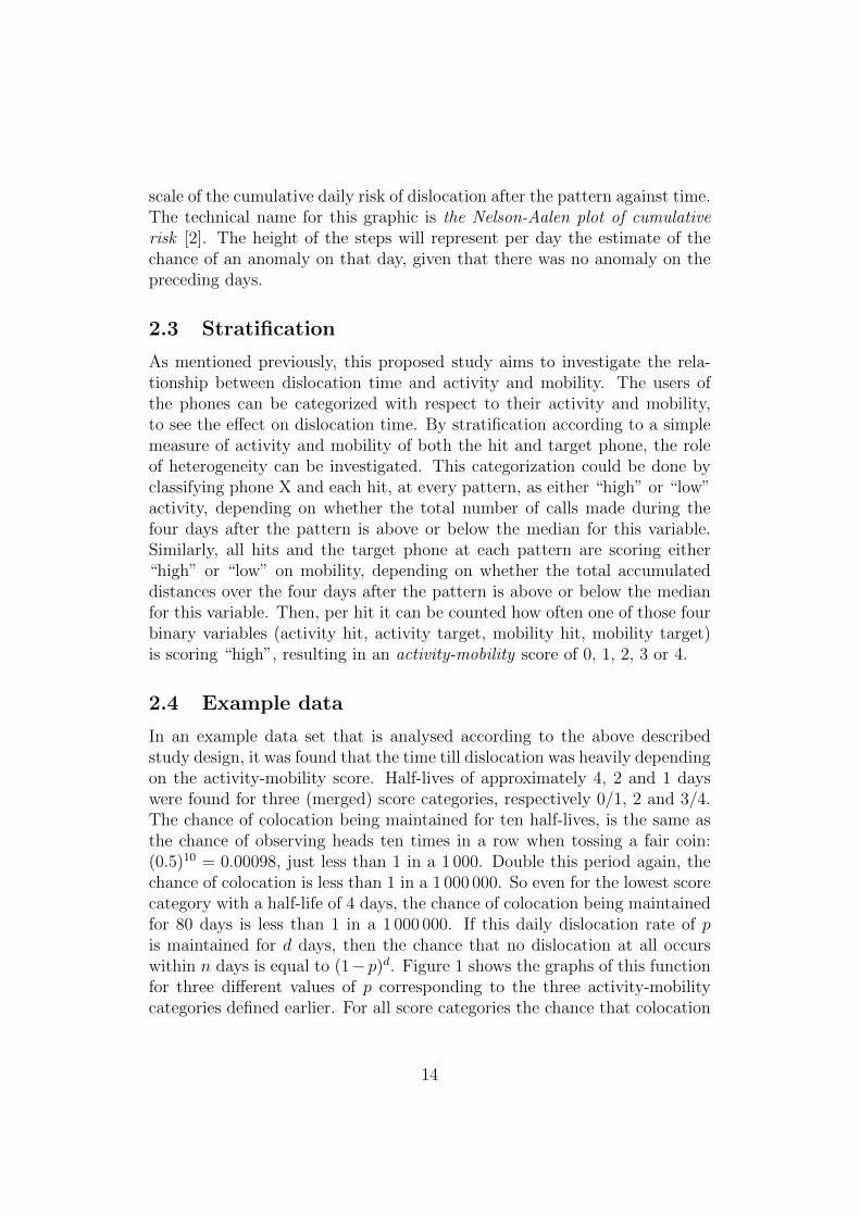
2.3 Stratification

As mentioned previously, this proposed study aims to investigate the rela-tionship between dislocation time and activity and mobility. The users ofthe phones can be categorized with respect to their activity and mobility,to see the effect on dislocation time. By stratification according to a simplemeasure of activity and mobility of both the hit and target phone, the roleof heterogeneity can be investigated. This categorization could be done byclassifying phone X and each hit, at every pattern, as either “high” or “low”activity, depending on whether the total number of calls made during thefour days after the pattern is above or below the median for this variable.Similarly, all hits and the target phone at each pattern are scoring either“high” or “low” on mobility, depending on whether the total accumulateddistances over the four days after the pattern is above or below the medianfor this variable. Then, per hit it can be counted how often one of those fourbinary variables (activity hit, activity target, mobility hit, mobility target)is scoring “high”, resulting in an activity-mobility score of 0, 1, 2, 3 or 4.

2.4 Example data

In an example data set that is analysed according to the above describedstudy design, it was found that the time till dislocation was heavily dependingon the activity-mobility score. Half-lives of approximately 4, 2 and 1 dayswere found for three (merged) score categories, respectively 0/1, 2 and 3/4.The chance of colocation being maintained for ten half-lives, is the same asthe chance of observing heads ten times in a row when tossing a fair coin:(0.5)10 = 0.00098, just less than 1 in a 1 000. Double this period again, thechance of colocation is less than 1 in a 1 000 000. So even for the lowest scorecategory with a half-life of 4 days, the chance of colocation being maintainedfor 80 days is less than 1 in a 1 000 000. If this daily dislocation rate of pis maintained for d days, then the chance that no dislocation at all occurswithin n days is equal to (1− p)d. Figure 1 shows the graphs of this functionfor three different values of p corresponding to the three activity-mobilitycategories defined earlier. For all score categories the chance that colocation

14

Figure 1: Chance of no dislocation by day d when daily dislocation rate isconstant, by three categories of activity and mobility of phone X and hit. Cutoff = 1/1000.

is maintained decreases in exponential fashion to zero, but how fast theapproach to zero occurs depends strongly on activity-mobility score.

2.5 Conclusion

With the study design that is proposed in this section, colocation-dislocationcan be empirically studied. To test whether or not dislocation is influenced bymobility and activity, a score can be assigned to each hit along to the amountof mobility and activity of the target and the hit phone. In an example dataset it was found that the time till dislocation was heavily depending onthe activity-mobility score, and that three different activity-mobility groupsresulted in half-lives of approximately 4, 2 and 1 days. From the fact thattime till dislocation is found to be affected by the activity-mobility score, onecan conclude that it is of utmost importance to take these two features intoaccount in future cases where the evidential value of colocating behaviour oftwo phones is studied. These findings furthermore imply, especially for hitsthat are in higher categories, that colocation for a very long period of daysoccurs rarely by chance.

15

2.6 Discussion

Within this section, it is discussed which fallacies that have led to miscar-riages of justice in the past are relevant, and which considerations have beentaken into account in order to prevent the same errors occurring again.

2.6.1 Tunnel vision

When Cell Site Analysis is used to assist investigators in a criminal investi-gation, one has to be aware of the problem of tunnel vision. Although thisfallacy has no relation with the use of mathematics or probabilities in courtand can occur in every criminal case, it is important to remain aware of thisoccurrence when the experiment is actually applied within the context of acriminal case. For the discussed cases of judicial miscarriages in the introduc-tion, tunnel vision was definitely a key factor in the conviction of Lucia de B.and Sally Clark. Both women were depicted as ruthless child murderers bylocal and national newspapers, which probably made it hard for the judgesto look at the evidence in an objective way. Findley & Scott (2006) statethat tunnel vision can lead to depraved consequences when it evolves in thecriminal justice system. They define this occurrence as a “compendium ofcommon heuristics and logical fallacies, to which we are all susceptible, thatlead actors in the criminal justice system to focus on a suspect, select andfilter the evidence that will build a case for conviction, while ignoring or sup-pressing evidence that points away from guilt” [7]. When investigators usetelephone data in their search for a suspect, tunnel vision can certainly be anissue. Once the investigators have their sights focussed on a person, it is al-ways hazardous that every favourable finding for the defendant is interpreteddifferently and revolved into something disadvantageous. It is therefore im-portant that an expert witness always questions the investigation methodsand takes a critical look at the path that is followed to arrive at a suspect.

2.6.2 Unlikely events are not impossible

Within statistics it is very common to report the p-value, and a low p-value isoften accepted as a ground on which one may reject the hypothesis that theevents occurred by chance. A p-value under 1 in 1000, is generally approvedas a legitimate reason to question whether the hypothesis of pure chance canbe rejected. However, one should bear in mind that occasionally very unlikelyevents do occur in this world. Think about Sally Clarke, who lost two babyboys to an unknown cause. An occurrence that is highly unlikely to take placedid occur. Findings that can be interpreted as highly unlikely can thereforebe a motivation for further analysis, but one should be careful in stating

16

definite conclusions. Further, a low probability for an event to occur, shouldnot be confused with the probability of innocence. For both Sally Clark asLucia de B., the public interpreted the (incorrectly calculated) extremely lowprobability for the events to happen naturally, as the probability that thedefendant might be innocent.

2.6.3 Large dataset

In order to execute the proposed study design, data must be available onmany phone records. One is probably working with a data set that can beconsidered very extensive. When a search is done in a large dataset, oneshould keep notion of some peculiarities that can take place with respectto the random match probability. This issue often arises in cases where atrace of DNA is found at a crime scene and it is attempted to calculatethe probability that a defendant randomly matches the found DNA. A casewhere a suspicious phone record is found around the time of a crime, dealsin a way also with a found trace at a crime scene, and investigators willhave to try to find a match. However, one should keep in mind that even anextremely low random match probability can lead to some random matcheswhen a search is performed in a very large data set. The amount of randommatches you expect can be counterintuitive. When you come across a randommatch probability for a certain event of one in 13 billion and a search isperformed among 600000 people, you already expect 13 random matches,since the number of comparisons you make is N(N − 1)/2, which in thiscase equates to 180 billion. However, when a profile is already present atthe start of the search, the number of expected random matches is equal tothe random match probability multiplied with the size of the dataset. Withthe proposed investigation methods, a suspicious phone profile is detectedand after that a search is performed among the phone records for a match.To expect a counterintuitive number of random matches is not the issue,but with the magnitude of the data set, one should still be careful wheninterpreting random match probabilities of one in a million.

17

3 Evaluating colocating phones

As mentioned previously, the second part of this thesis explores the possibil-ity of statistically quantifying the closeness of the paths followed in time andspace by two mobile phones. The method developed in this thesis can beapplied to test the hypothesis whether two phones are probable to be usedby the same person. It is probable that phones that are used by a criminalwill only colocate over a short period of time, making it therefore difficultto say anything conclusive about their connection. Within this section sta-tistical methods are explored to quantify the visual impression of colocatingbehaviour. To introduce the methodology, data is simulated on the behaviourof a person moving around and making phone calls.

3.1 Texas sharpshooter

Before the methodology is further explained, it is important to weigh in mindwhether the selection of two phones for comparison is not facing the so calledTexas sharpshooter fallacy. The name is derived from the story of a Texanfarmer, who painted a target on the side of his barn around a previous shotbullet hole. Afterwards, he was considered a competent sharpshooter, an ob-vious fallacious reasoning. Within a research or investigation, the problem ofTexas sharpshooter often arises when a pattern is presumed to exist betweenpieces of data that actually have no connection with one another. Thompson(2009) studied the occurrence of the Texas sharpshooter fallacy within theforensic field and concludes that “DNA analysts tend to underestimate thefrequency of matching profiles (and overestimate likelihood ratios) by shiftingthe purported criteria for a ‘match’ or ‘inclusion’ after the profile of a suspectbecomes known” [12].

When the closeness of two telephones in time and location is tested, the prob-ability is calculated that a certain event occurred by chance, which is similarto research questions in DNA or other forensic matching methods. When thebroader context is disregarded and one is intensively focussed on a particularoutcome, calculations like this can be fallacious. One has to be careful thatno significance is assigned to random results by considering it retrospectivelyin an exorbitantly narrow context. When an investigative unit starts theirsearch for colocating phones without specifying hypotheses prior to the gath-ering of the data, and questions the significance of the found patterns afterthey are detected, this can be a hazardous consecution of proceedings andone could question such a procedure. It would be illogical to test a hypoth-esis on the same data that was used to generate that hypothesis. However,

18

when the study is executed that is proposed in the previous section, phonesare included in the study based on patterns, covering at most four days. Fol-lowing up initial hits in time allows the researcher independently to decidewhether or not the initial pattern of colocation is due to chance. When hitsare followed for a few days and many phones seem to dislocate, that meansthat a small part of the data already leads in the direction of longer colo-cating phones. The findings of half-lives of 1, 2 and 4 days suggest that anexplanatory analysis based only on a small bit of the data can already leadinvestigators towards colocating phones. The methodology introduced in thecurrent section can be applied on a separate, independent part of the data,with many more subsequent days. The statistical analysis on an apparentlycolocating pair of phones can therefore be seen as an independent confirma-tory analysis on a long time history. Thus, there is no need to worry aboutthe Texas sharpshooter fallacy.

3.2 Aim

When records of the calls of two phones are obtained, it is possible to visuallyrepresent the path of the two phones both in time and location. In a largedata set consisting the phone records of many phones, it could be foundthat the pattern of times and locations of the calls of two phones together isconsistent with the two phones being carried by one person. This similaritycould of course be a coincidence, but this study aims to introduce a methodthat can test whether or not two paths followed by the two phones are so closetogether that the hypothesis that they are carried by two different personscan be ruled out. In other words: how large is the statistical likelihood ofchance colocation?

3.3 Visualisation

Before the method is further explained, it is important to obtain a solidunderstanding of the idea behind the developed methodology. With a numberof graphs it is attempted to visualise a person moving around making phonecalls and to envision what it looks like when two phones are colocating for aperiod of time. In order to make these graphs, a little data set is simulatedwhere we imagine a person moving around throughout an area of 100 by 100kilometres, commonly visiting 15 locations within that area. Imagine thisperson moving not randomly, but along a fixed collection of trips. For animaginary individual, a pattern of 30 randomly chosen consecutive trips issimulated from the trips that are displayed in Figure 2a. Trips where hestays at the same location for a while are also included.

19

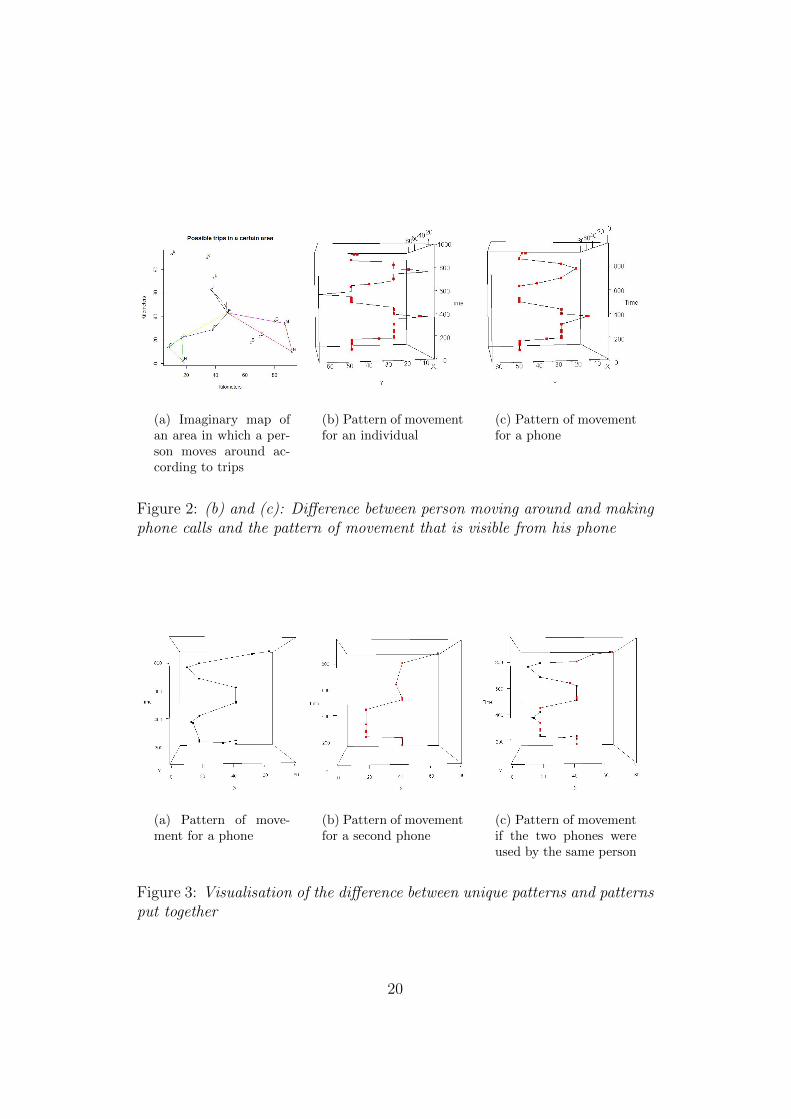
(a) Imaginary map ofan area in which a per-son moves around ac-cording to trips

(b) Pattern of movementfor an individual

(c) Pattern of movementfor a phone

Figure 2: (b) and (c): Difference between person moving around and makingphone calls and the pattern of movement that is visible from his phone

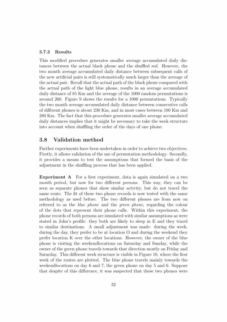
(a) Pattern of move-ment for a phone

(b) Pattern of movementfor a second phone

(c) Pattern of movementif the two phones wereused by the same person

Figure 3: Visualisation of the difference between unique patterns and patternsput together

20

Assuming a traveling speed of 60 kilometres per hour, it is possible to producea 3d plot of the path he has followed, putting the location of the individualtogether with the time he would be there. During his movement he mightmake some phone calls, indicated with a red dot in Figure 2b. However, exactinformation on the whereabouts of individuals is not available when one isworking with phone record data. Figure 2c displays the pattern of the sameindividual as Figure 2b, but then by only taking the location of his phonecalls into account. Thus, when the location (longitude and latitude) of thecell tower that picked up the signal of the calls is taken into account togetherwith the time of the calls and subsequent calls are connected by straightlines, it is possible to produce 3d plots of the path a phone has made, or evenof the path a pair of phones has made.

As mentioned before, the methodology developed in this thesis is built uponthe assumption that people will occasionally carry two phones around. Imag-ine a business man who wants to separate business from his personal activ-ities, or a criminal who uses an anonymous phone in the preparation of acrime. In such cases, one could encounter phone patterns as displayed inFigure 3a and 3b. At first sight, these patterns do not necessarily look verysimilar, but when the two phones are put together on a string one observes aphone pattern that is consistent with what a phone pattern would look likeif the two phones were carried by one person. Figure 3c shows the path thatwould have been followed if the two phones were used by the same person.The line connecting the points follows the time sequence of the combinedrecord of calls. The visual impression of this 3d plot is that the red andblack points fit together rather nicely onto a single path. When both phonesare active, they are in the same location. Occasionally one of the phones“travels” to another area, without the other phone showing activity. Thetwo phones are never making a phone call far apart in space but close to-gether in time. If the two phones are in the same hands, every move thatwould have been made is perfectly feasible. The method that will be furtherexplained in this chapter, aims to determine the significance of this observedconnection between phones, in order to potentially increase the reliability ofpresented evidence in court.

3.4 Data simulation

To introduce the developed method data is simulated for a person movingaround and making phone calls with two different phones over a period oftwo months (61 days), in an area of approximately 50 by 100 kilometres.

21

Let’s call him John. With the model that is used in the data simulation, itis attempted to make John’s profile as realistic as possible. Several aspectswere taken into account:

• It is likely that a person who is moving around will frequently go backto the location he lives. Therefore, a location is chosen that he willvisit frequently and where he spends most of his nights. John lives inlocation E and when it gets later than 11.00 pm, he is more likely totravel back to location E.

• Figure 4a displays John’s possible routes during a week day. The ideais that John has a weekly structure in his movements due to his work,on a work day he moves around locations that are southwest from hishome (locations C, O, H, F). From this four week locations, John visitslocation O most often. With the selection of his next move, there isalso a small probability that he travels to locations that he mostly visitsduring the weekend, but 9 times more weight is given to trips that arein the direction of his work.

• During the weekend John mostly travels in a northwest direction. Itmakes sense that a person travels to different locations during the week-end than during the week. Perhaps he visits family and friends, orthere are some entertaining activities that he likes to do on a day offwork. Figure 4b displays John’s possible movements during the week-end. Throughout the weekend there is also a small probability thathe will visit the locations that are part of the weektrips, but again,with the selection of his next move, much more weight is given to theweekendtrips. On top of that, from all possible locations that are partof the weekendtrips, more weight is given to location K, his favouriteweekend location.

• During the night-time, between the hours of 0.00 and 8.00 am, Johnstops moving and stays in the same location. Most of the nights hestays in location E, but occasionally he spends the night somewhereelse. During the night the calling frequency is very low; there are justa few phone calls made in the night-time over the period of 61 days.

• As mentioned before, John is carrying around two mobile phones anduses them equally frequent. During the day, he switches randomly fromone phone to another.

The simulated movements of John and the phone calls he makes are dis-played in Figure 6a and 6b, where the second graph shows the same sequence

22

(a) (b)

Figure 4: Visualisation of possible weektrips and weekendtrips

(a) Two months (b) Zoomed in on the first week

Figure 5: Visualisation of the simulated movements and phone calls over atwo month period

23

of movements and calls, but then zoomed in on the first week of the 61 daysperiod. The colours of the dots indicate which phone he was using. Thedataset with the time and location of the calls of the two phones will be usedto explain the methodology that is developed to test the closeness of twopatterns of phones. The data is now simulated in a way that the phone callsof the two phones are actually simulated from a sequence of movements ofone person. It is important to keep notion of the fact that criminal investi-gators will separately come across the phone records of the red and the blackphone. When they put the two phone records together, they show a paththat could be travelled by one person, from which the suspicion arises thatthe two phones might belong to the same person.

3.5 Methodology

When investigators come across two phones of which they suspect that theyare used by the same person, it would be ideal if they can create a largesample of pairs of different persons, who are independently making similarmovements and using their phone in a similar way. With such a sample itwould be possible to compare the paths of the two phones to a large numberof phones that are carried by different persons. Defining these notions inorder to collect such a sample from the available phone records can be adifficult task that will cost a lot of time and money. However, when dataof only two phones is available, “time” provides us with a unit of repetitionwith which we can construct an artificial sample of phone histories of similarphone users.

3.5.1 Permutation tests

In general, a permutation test can be used to obtain the distribution of atest statistic, by calculating all possible values of this test statistic underrearrangement of the labels of the observed data points. This test is oftenapplied to test the hypothesis whether or not two different groups of personsor objects actually come from the same distribution. For two groups a certaintest statistic can be of interest (for instance the difference of the two samplemeans), and when this test statistic in the original grouping significantly dif-fers from the test statistics of all possible rearranged groups, the conclusioncan be drawn that the original group label matters and the null hypothesisthat these groups come from the same distribution can be rejected.

When the paths of two phones are compared, there is no question of com-paring two groups of people, but the permutation methodology can still be

24

appropriate for the case at hand. The path that is formed by the recordsof a phone can be seen as a collection of days, and for this experiment thedays within a path will be shuffled in order to construct an artificial phonehistory. The order of phone calls within a day will be retained, but the dayswill be rearranged. The path that is created of a “new” phone, can be seenas coming from a phone that makes similar movements as the original phone,uses the phone equally intensively, spends the night at the same location, andso on. With regard to the two phones of interest, one questions the fact ifthey are used by different persons, but when a comparison between the pathof one phone with a shuffled path of another phone is made, this can be seenas a comparison between two phones that are known to be in in differenthands.

How well the two telephone records fit together, can be seen as the statis-tic of interest. Defining the fit of two mobile phones, and determining their“closeness”, will be discussed later in this section. If two phones are carriedby different persons, it is expected that rearranging the days of one phone,will not change the closeness of the two phones. In other words, if two phonesare not in use of the same person, and the similarity in the paths only arisesby chance (for instance because two people live in the same building andwork in the same area), shuffling the days of the path of one phone shouldyield a path that is still equally similar to the path of the other phone. Ifrearranging the days of one phone affects the test statistic (the closeness ofthe two paths) significantly, it can be concluded that the original closenessof the two paths is special, and a logical explanation for this could be thatthe two phones are in use of the same person. Thus, when the actually ob-served closeness is much smaller than the closeness of almost all the shuffledpaths, we conclude that the observed closeness is highly improbable underthe hypothesis that the phones are in different hands.

3.5.2 Measuring closeness

The statistic that is used to measure the closeness of two paths is evidentlya point of interest that can be discussed. Before this is further elaborated, itmust be noted that different kinds of closeness between paths of phones canbe detected. In the first case, one can imagine that a person is carrying twophones for two different activities (for instance business and private) andrigorously separates these activities into different time periods every day.Then, the person will use one phone for a period of time during a certainactivity, and then switches to the other phone, putting the first phone downfor a while, then switches to the first phone again, and so on. When the two

25

paths are put together, this kind of use of two phones will result in a patternthat has activity of one phone combined with a lull in activity of the otherphone and vice versa. The two paths will link up at the switches betweenthe two activities. On the other hand, one can also imagine that a person iscarrying two (or maybe more) phones, and uses them both during the sameactivity, but for communication with different groups of contacts. Thus, theuse of one phone will go together with the use of another phone. Whenthe two paths are put together, this kind of use will result in a pattern ofactivity of both phones, followed by a lull in activity of both phones, followedby activity of both, and so on. This difference is important when a measureof closeness is developed.

To compare the paths of two phones and measure how well the patterns fittogether, the distance that is covered every time a switch is made on thesame day between one phone to the other is calculated. A switch occurswhenever two subsequent calls on the same day in the combined call recordsof two phones are made by two different phones. Over all the days, thesedistances are accumulated and provide a measure of closeness of the twopaths. A second statistic that is studied to determine how well the pathsof two phones fit each other is the number of anomalies that occur whenthe paths of two phones are combined. As stated in the introduction, ananomaly is defined as the occurrence of two calls on two phones close in timebut distant in location. An anomaly is said to have occurred when two callsare made within 15 minutes of one another at distances (of the respectivecell towers) of at least 25 Km.

3.6 Results

1. In this section results regarding the average accumulated daily distanceare discussed. Recall that the sum of all distances between the twophones is added up over all switches, within the same day, between thetwo phones. The two phones will be referred to as the black phone andthe red phone, according to the colour of the dots that represent theirphone calls.

• Actual: for the 61 days, the sum of all distances between locationsof phones when a switch is made between one phone to anotheris 5192 Km. The average daily accumulated distance between thelocations of cell towers involved in subsequent calls by each of thetwo phones is around 85 Km.

• Shuffled: a permutation test is applied, whereby the match of the

26

actual history of the black phone is matched to the history ofthe red phone after a random permutation of the days. This wasdone for 1000 random permutations of the days of the red phone.Figure 6 shows a histogram of the resulting two month averageaccumulated daily distance between the black and the red phonefor these 1000 random permutations. Typically the two monthaverage accumulated daily distance between consecutive calls ofdifferent phones is about 260 Km, and in most cases between 220Km and 300 Km.

2. When we take a look at the second statistic to measure the closeness ofthe paths, namely the number of anomalies, similar results are found.

• Actual: in the three month period that has been studied, theblack and red phone never exhibit an anomaly defined earlier inthis chapter. This result is quite logical since the two phonesare simulated from the movements of one person. However, alsowhen investigators find two phones of which they suspect thatthey are used by the same person, no anomalies will be detectedin the original comparison of the paths of the two phones, sincean anomaly is defined in such a way that it is a strong indicatorof the phones not being used by the same person.

• Shuffled: all of the 1000 shuffled histories exhibit a substantialnumber of anomalies. Figure 7 shows a histogram of the numberof anomalies found in a two month comparison between the blackphone history and 1000 permutations of the red phone history.Typically around 90 anomalies are detected, and the largest partof the permutations show between 60 and 120 anomalies.

As seen before, it is possible to plot two phone paths in a 3d box, to seehow they fit together and to get an impression about the difference betweenthe original path and a shuffled path. Figure 8 shows (a) the actual path ofthe black and red phone together and (b) the path of the black phone withone of the 1000 permutations of the red days. It can be concluded that thecomparison between the black phone with a permutation of the red phonelooks messier, but to see the difference more clearly one can take a look atFigure 8c and 8d. This plot zooms in on (c) the first 2 days of the actual callsof the black and red phone and (d) the actual calls of the black phone on thefirst 2 days of the three month time period, together with the calls of the redphone on 2 other days selected at random in the two month period (one of

27

Figure 6: Daily average total distances between consecutive calls of the blackphone and 1000 permutations of the red phone in a 2 month period

Figure 7: Total accumulated anomalies between consecutive calls of the blackphone and 1000 permutations of the red phone in a 2 month period

28

(a) Actual (b) Red daysshuffled

(c) Actual (d) Red daysshuffled

Figure 8: (a) and (b): Black phone and red phone on a two month period, (c)and (d): Black and red phone on the first two days of the two month period

the random permutations). Within the actual path the calls of the black andred phone fit together in such a way that it is feasible that they are carriedby the same person. Within the shuffled path some strange movements andeven some anomalies are detected if the two phones were in the hands of thesame owner.

A shuffled, artificial phone record can be seen as a typical history of the callsmade by a phone user very similar to the owner of the red phone. As statedbefore, the new phone spends a similar amount of time in exactly the sameplaces as the red phone, it is used just as intensively, it has been taken on thesame journeys, and so on. Since it is known that the history of this phone isartificial, comparing it to the black phone results in a combined pattern thatone would expect when the two phones are in different hands. Putting theblack phone record together with a shuffled red phone record results in cleardislocations (anomalies) on several days, indicating that the original pathsof the two phones do show a special connection.

29

3.7 Reflection on the methodology and an adjustment

Up until now an artificial sample is created of pairs of phones carried bydifferent persons. Within each pair, one phone is similar to the black phone,the other phone is as similar as possible to the red phone. With use of permu-tation methodology the question is addressed whether the actual black andred combination looks like one of these pairs of phones in different hands,or whether it looks like a pair of phones in the same hands. This is sta-tistically quantified by fixing a numerical measure on the paths of a pair ofphones. One can imagine sophisticated measures of the degree of erraticismof the joint path, or equivalently of the degree of mismatch between the twopaths. So far a measure of closeness has been studied that is simple andquite directly corresponds to what can be seen when looking at the graphs.Importantly, this measure can be computed easily and rapidly, so it can becomputed for many pairs of phones. First, the sum of all distances betweenthe locations of cell towers is calculated between pairs of calls of the twophones which are adjacent in time (and on the same day). If two phones arein different hands, it is expected that from time to time they make phonecalls close together in time but in locations which are far apart from oneanother. On the other hand, if two phones are in the same hands and areused close together in time, there cannot be a large distance between the twolocations at which they are used. A second measure that is taken into ac-count is the number of dislocations between the two phones. Both measuresare considered in a comparison between pairs of phones (an actual pair, andmany artificial pairs formed by shuffling the days of one of the phones) thatare similar with respect to the length of time they are followed and theiractivity and mobility.

3.7.1 Adjusting shuffling

A logical point of critique for this method is that human life shows manypatterns and regularities and that the closeness of the paths of two phones isautomatically influenced when the days of one phone are randomly shuffledwithout this patterns taken into account. When measuring the correlationbetween the locations of calls made by different phones on different days, it ispossible that a large correlation between the locations is detected because theowners are making similar movements from one day to another. When thedays are shuffled randomly, the extremely strong weekly rhythm to humanbehaviour is not taken into account. One can imagine that especially in a city,the movements of two persons on week days versus weekend days are different,as is also taken into account when the data of a person moving around was

30

(a) Only the week days are shuffledwith each other

(b) Actual (c) Red days shuf-fled

Figure 9: (a) Daily average total distances between consecutive calls of theblack phone and 1000 permutations of the red phone in a 2 month period -week days shuffled; (b) and (c): Black and red phone on the first two days ofthe two month period

simulated. When the artificial red path is created by shuffling all the 61 dayscompletely at random, the behaviour of the black phone on some week daysis sometimes juxtaposed to the red phone on weekends. Systematic weeklypatterns in human movements and behaviour do exist, such that randomlyshuffling all the days possibly produces misleading results.

3.7.2 Method

To take care of this problem a new method of rearranging the days of the redphone is implemented. The experiment is repeated, but now all Mondays,all Tuesdays, all Wednesdays, and so on, are shuffled independently, andseparately from one another. This way, the distance between calls of theblack phone and calls of the artificial red phone are measured on the samedays of the week.

31

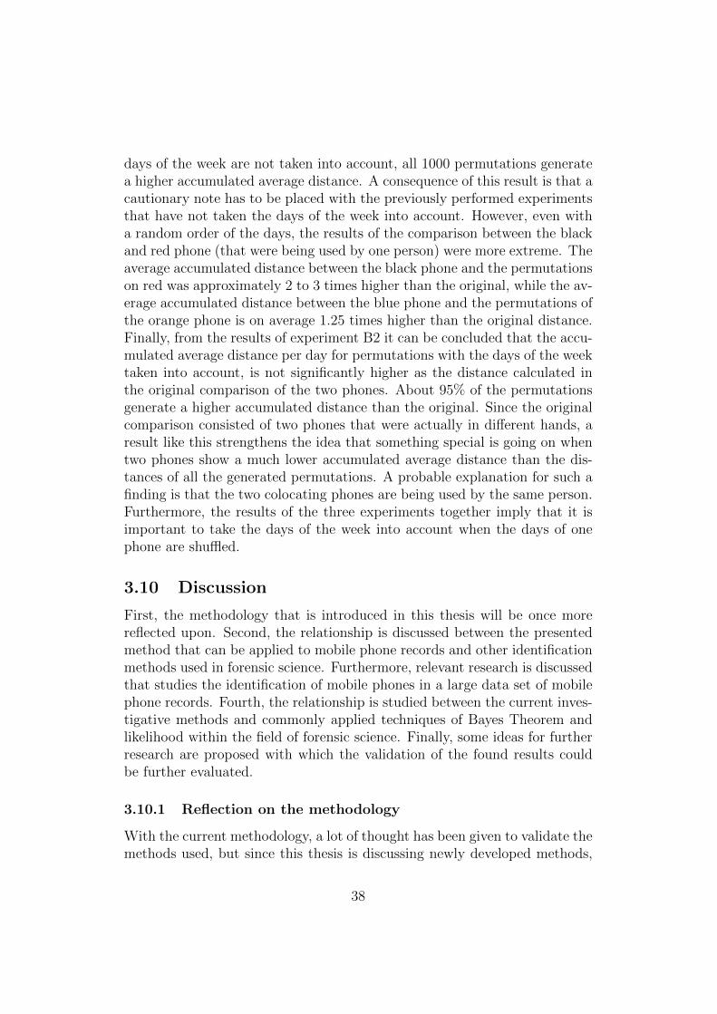
3.7.3 Results

This modified procedure generates smaller average accumulated daily dis-tances between the actual black phone and the shuffled red. However, thetwo month average accumulated daily distance between subsequent calls ofthe new artificial pairs is still systematically much larger than the average ofthe actual pair. Recall that the actual path of the black phone compared withthe actual path of the light blue phone, results in an average accumulateddaily distance of 85 Km and the average of the 1000 random permutations isaround 260. Figure 9 shows the results for a 1000 permutations. Typicallythe two month average accumulated daily distance between consecutive callsof different phones is about 230 Km, and in most cases between 180 Km and280 Km. The fact that this procedure generates smaller average accumulateddaily distances implies that it might be necessary to take the week structureinto account when shuffling the order of the days of one phone.

3.8 Validation method

Further experiments have been undertaken in order to achieve two objectives.Firstly, it allows validation of the use of permutation methodology. Secondly,it provides a means to test the assumptions that formed the basis of theadjustment in the shuffling process that has been applied.

Experiment A For a first experiment, data is again simulated on a twomonth period, but now for two different persons. This way, they can beseen as separate phones that show similar activity, but do not travel thesame route. The fit of these two phone records is now tested with the samemethodology as used before. The two different phones are from now onreferred to as the blue phone and the green phone, regarding the colourof the dots that represent their phone calls. Within this experiment, thephone records of both persons are simulated with similar assumptions as werestated in John’s profile: they both are likely to sleep in E and they travelto similar destinations. A small adjustment was made: during the week,during the day, they prefer to be at location O and during the weekend theyprefer location K over the other locations. However, the owner of the bluephone is visiting the weekendlocations on Saturday and Sunday, while theowner of the green phone travels towards that direction mostly on Friday andSaturday. This different week structure is visible in Figure 10, where the firstweek of the routes are plotted. The blue phone travels mainly towards theweekendlocations on day 6 and 7, the green phone on day 5 and 6. Supposethat despite of this difference, it was suspected that these two phones were

32

(a) Person 1 - blue phone (b) Person 2 - green phone

Figure 10: (a) and (b): Two persons moving around and making phone callswith a different week structure

(a) Person 1 - blue phone (b) Person 3 - orange phone

Figure 11: (a) and (b): Two persons moving around and making phone callswith the same week structure

33

(a) Random shuffle, dif-ferent week structure.Original: 428

(b) Random shuffle,same week structure.Original: 363

(c) Weekly shuffle, sameweek structure. Origi-nal: 363

Figure 12: Results experiment A, B1 and B2

being used by the same person. A permutation test could be applied to testwhether the original distance between the two phones is very different fromthe distance between the blue phone and 1000 permutations on the order ofthe days of the green phone. Since we know in advance that the phones areactually not being used by the same person, we do not expect the permuteddistances to deviate much from the original distance. The same measure ofcloseness is calculated: the cumulative distance that is covered every time aswitch is made on the same day from one phone to the other. Over this twomonth period, the total accumulated distance is 26108 kilometres. This is afairly high number, it would mean that a person that is using both phonesis traveling more than 428 kilometres per day. The order of the days of thegreen phone is randomly permuted 1000 times, and for each permutation themeasure is calculated again. Around 93% of the permutations result in ahigher accumulated distance than the original. A histogram of the resultscan be found in Figure 12a. This result confirms the expectation that thepermuted distances are not extremely different from the original distancethat was covered if the phones were being used by the same person. Notethat the two owners of the phones in this experiment did not have the sameweek structure.

Experiment B

1. In the next experiment one of the persons for which data was simu-lated is now compared to a third simulated person (owner of the or-

34

ange phone), that moves around according to the same week structure.They both travel weekendtrips mainly on Saturday and Sunday, andweektrips during the week. With this comparison, the original distanceis calculated over days that have mainly the same week structure, asseen in Figure 11. If one person would use both phones, the originalaccumulated distance is 22178 kilometres, an average of approximately363 kilometres per day. Again, 1000 permutations are randomly gener-ated on the days of the orange phone, where these permutations do nottake the days of the week into account. A total of 100% of the permu-tations generate a higher accumulated distance that the original, thehistogram of the results is displayed in Figure 12b.

2. With a final experiment, we will try to determine the effect of shufflingthe days of the orange phone not randomly, but by the days of theweek. Again 1000 permutations are generated on the order of the daysof the orange phone, shuffling Mondays only with Mondays, Tuesdayswith Tuesdays etc. With this method, around 95% of the permutationsgenerate a higher accumulated distance that the original. Again, thehistogram of the results is seen in Figure 12c.

In order to draw conclusions from these experiments, it is important tothoroughly understand the difference between the three experiments. Table2 to 6 show the original comparison and an imaginary permutation for allthree experiments. Note that the permutations of experiment B2 are notrandom: the difference between the numbers of the days that are comparedwith each other is divisible by 7.

3.9 Conclusion

Within this thesis, methodology is introduced to test for a pair of phoneswhether the observed colocation could have occurred by chance. More pre-cisely, with use of this statistical test, the probability can be estimated thata pair of phones similar in all respects to the present pair, but in differenthands, would show, by chance, such a pattern of colocation as was actuallyobserved. The first important decision was taken on the measure of close-ness of the paths in time and location of two phones, which is a matter ofjudgment. This measure has to be intuitively easy to understand and easyto calculate on available call records.

The colocation of pairs of phones is investigated, comparing the actual dailyaccumulated distance between switches with what one would expect by chancefor similar phones in separate hands. Data is simulated of one person moving

35

Table 2: Original Comparison Experiment A

Phone 1 Day 1 Day 2 Day 3 Day 4 Day 5 Day 6 Day 7Monday Tuesday Wednesday Thursday Friday Saturday Sunday

Week Week Week Week Week Weekend Weekend

Week Week Week Week Weekend Weekend WeekPhone 2 Monday Tuesday Wednesday Thursday Friday Saturday Sunday

Day 1 Day 2 Day 3 Day 4 Day 5 Day 6 Day 7

Table 3: Possible Permutation Experiment A



Week Week Week Week Weekend Week WeekPhone 2 Sunday Monday Tuesday Thursday Saturday Thursday Wednesday


Table 4: Original Comparison Experiment B1 & B2



Week Week Week Week Week Weekend WeekendPhone 2 Monday Tuesday Wednesday Thursday Friday Saturday Sunday


Table 5: Possible Permutation Experiment B1



Weekend Week Week Week Weekend Week WeekendPhone 2 Saturday Tuesday Friday Thursday Sunday Tuesday Saturday


Table 6: Possible Permutation Experiment B2



Week Week Week Week Week Weekend WeekendPhone 2 Monday Tuesday Wednesday Thursday Friday Saturday Sunday


36

around, making phone calls with two phones. Permutation methodology isused to create an artificial sample of phone histories that are similar to thehistory of one of the phones. The idea is that if two phones are unrelated,mixing up the days of the history of one of the phones generates a new his-tory of a phone of very similar behaviour to the original.

When the time of the calls together with the location of the cell tower sectorthat picked up the call is taken into account, it is decided to take the averageaccumulated distance between switches, as well as the number of anomalies,as a measure of closeness. With this data it is possible to make 3d plots,to get a visual impression about the way two telephone records fit together.Data was simulated over a time period of two months of the calls of the blackphone and the red phone. From the 3d plot of the actual histories, it canbe concluded that the black phone and red phone fit well together on a longstring, with no strange movements (no anomalies) if the phones were carriedby one person. When the path of the black phone is put together with anartificial path of the red phone, clearly a different picture arises. For theaverage daily accumulated distance, as well as the number of anomalies, all1000 permutations show significantly higher values. After a modification ofthe procedure of shuffling, where the days of the light blue phone are sys-tematically shuffled by the days of the week, the average daily accumulateddistance decreases somewhat, but still remains highly significant. Still allpermutations give a number about 2 to 3 times as high as the average dailyaccumulated distance in the actual comparison.

Finally, three experiments were performed to validate the method used tocompare phone records. The aim of the experiments was to study the conse-quences of applying the developed permutation methodology on two phonesthat are known to be not being used by the same person and to determinethe importance of taking the days of the week into account when the order ofthe days of one phone is permuted. To create a pair of phones that are knownto be in different hands, two persons are simulated moving through space,both using a phone. First, two persons are generated that travel amongthe same locations, but have a different week structure. From the results ofexperiment A it can be concluded that comparing these two phone recordsthat are actually in different hands results in a high accumulated averagedistance per day, and that 1000 permutations generally do not result in sig-nificantly higher distances. Experiment B1 shows that a comparison betweentwo phones that are still in different hands, but move around on the same dayof the week, results in a considerably lower accumulated average distance perday. When the order of the days of one of the phones is permuted and the

37

days of the week are not taken into account, all 1000 permutations generatea higher accumulated average distance. A consequence of this result is that acautionary note has to be placed with the previously performed experimentsthat have not taken the days of the week into account. However, even witha random order of the days, the results of the comparison between the blackand red phone (that were being used by one person) were more extreme. Theaverage accumulated distance between the black phone and the permutationson red was approximately 2 to 3 times higher than the original, while the av-erage accumulated distance between the blue phone and the permutations ofthe orange phone is on average 1.25 times higher than the original distance.Finally, from the results of experiment B2 it can be concluded that the accu-mulated average distance per day for permutations with the days of the weektaken into account, is not significantly higher as the distance calculated inthe original comparison of the two phones. About 95% of the permutationsgenerate a higher accumulated distance than the original. Since the originalcomparison consisted of two phones that were actually in different hands, aresult like this strengthens the idea that something special is going on whentwo phones show a much lower accumulated average distance than the dis-tances of all the generated permutations. A probable explanation for such afinding is that the two colocating phones are being used by the same person.Furthermore, the results of the three experiments together imply that it isimportant to take the days of the week into account when the days of onephone are shuffled.

3.10 Discussion

First, the methodology that is introduced in this thesis will be once morereflected upon. Second, the relationship is discussed between the presentedmethod that can be applied to mobile phone records and other identificationmethods used in forensic science. Furthermore, relevant research is discussedthat studies the identification of mobile phones in a large data set of mobilephone records. Fourth, the relationship is studied between the current inves-tigative methods and commonly applied techniques of Bayes Theorem andlikelihood within the field of forensic science. Finally, some ideas for furtherresearch are proposed with which the validation of the found results couldbe further evaluated.

3.10.1 Reflection on the methodology

With the current methodology, a lot of thought has been given to validate themethods used, but since this thesis is discussing newly developed methods,

38

it is important to continue evaluating the methodology and placing caution-ary notes with some of the results. When permutation tests are used, onehas to be aware of the possibility that the statistic of interest is increasingsignificantly because of other factors than the similarity of the original com-parison. The results of this thesis for instance imply that it is importantto take the week structure that exists in human movement patterns into ac-count when the order of the days of one phone is shuffled. For a comparisonof two phones that are not in the same hands, a random shuffle generatesaverage daily accumulated distances that are much higher than the original.A shuffle where one takes the day of the week into account generates reason-ably similar distances as the distance in the original comparison, which is astrong indicator that not taking the days of the week into account pushesup the distance measure automatically. However, the found percentage of95% is still fairly high, indicating that it will be necessary to search for otherconfounding factors that haven’t been thought of. Furthermore, it wouldbe interesting to study if the solution that was thought of to deal with thisweekly rhythm is optimal. To see what the results are when for instance notdays but whole week blocks are shuffled, would be worth knowing.

A critical note has to be placed with the choice of the distance measure. Upuntil now it is decided to look at the average accumulated daily distance be-tween switches, but one could think of more advanced methods to comparethe closeness of two paths in time and space. It will be interesting to investi-gate alternative distance measures and see if similar results can be found fordifferent distance measures. As stated in the beginning of this chapter, dif-ferent kinds of usage of two phones can be thought of. The chosen distancemeasure can lead to problems when a person is not using his two phonesrandomly during the day, switching randomly from one phone to the other,but uses them both for a period of time followed by a lull in activity, againfor both phones. When a person is carrying two (or more) phones and usestwo phones for the same activity, one can imagine that the two phone recordsseem highly related. Every day, both phones show activity during the samehours of the day and the cell towers that pick up the phone calls of the twophones are not far apart. To be able to statistically quantify the closeness ofthe two paths followed in time and space in situations like this, it is impor-tant to choose a distance measure that will go up when the history of onephone is compared to 1000 permutations on the history of the other phone.However, the original comparison will show a high number of switches perday, since the use of one phone is combined with the use of the other phone.The distances between the switches will not be very large, but a large numberof switches could result in a high average accumulated daily distance. Even

39

more so when one is taking into account that it is possible that a person isstaying put at one place, but the phone calls of his two phones are picked upby different cell towers around him, making it look like he is on the move.When the order of the days of one phone is shuffled, this block of activitywill be compared to a random other day of the other phone. It is very wellpossible that this random other day shows activity of the other phone ina different time period of the day. That way there are very few switches,generating a low average accumulated daily distance. A possible solution forhis problem is to take the average distance among switches instead of theaccumulated distance.

3.10.2 Relationship to other identification methods in forensic sci-ence

This section studies the relationship between the new investigative methodsthat can possibly be applied to mobile phone records and other disciplinesconcerning identification methods in the field of forensic science. The processof detecting perpetrators by investigating phone records bears much resem-blance to other kinds of evidence that are often presented in court. In away, this investigative method aims to analyse whether a phone pattern canbe matched to a person in a similar way a fingerprint expert compares thefingerprint found at the crime scene to the suspect’s print. In both situa-tions one is trying to determine the probability that the found conformity isdue to chance. Fenton & Neil (2012) introduce a way to address all proba-bilistic match evidence and discuss common fallacies that affect probabilisticreasoning with regard to evidence. They state that every branch of foren-sic matching that is based on some properties of people, follow the sameunderlying principles:

• “Every person has a ‘profile’ (defined by the area of forensics) that canbe measured by some defined procedure.

• In certain circumstances a person leaves a ‘trace’ (or ‘print’) of thisprofile.

• In certain circumstances we can measure the profile of the trace thatwas left.

• There is a criterion for determining whether a trace profile matches theprofile of a person.” [6]

The calls that a person makes can be seen as a person’s profile. Collecting the

40

phone records from the network providers, including the time and location ofall the calls made by a phone, is thereby the defined procedure that measuresthe profile. A small discrepancy exists between this approach and otherareas of forensic matching, since every phone has a profile, but a personcan carry multiple phones and thus have multiple profiles. A phone recordis therefore not matched to another person, but to another phone record.When one of the phones is registered to a known person, it is concluded thatthe anonymous phone belongs to that person as well.

Furthermore, the phone record of the phone that is found to behave in asuspicious way around the time of the assassination can be seen as a possibletrace that is left by the perpetrator. This part of the approach does notdiverge much from other forensic matching methods, such as fingerprints.People leave their fingerprints with almost every move they make, but whena fingerprint is found around a crime scene, this can be an indication thatthe print comes from the perpetrator. People that are frequent callers leavea lot of ‘phoneprints’ behind as well but when the print is found in such away that the phone shows activity around a crime, suspicion rises that theprofile can be attributed to the perpetrator.

The last point mentioned by Fenton & Neil (2012) is essential with respectto developed methodology. The first part of this thesis proposes a studydesign to study the likelihood of two phones colocating for a longer periodof time, and the second part quantifies the closeness of two paths by the useof permutation methodology. These new investigative methods attempt todefine a criterion for determining whether a trace profile matches the profile ofa person, or in this case the profile of another phone record. Steps have beentaken toward validation of these new methods. However, the reliability ofnew methods such as these remains open for discussion. Future experimentsare required to assess this matter and add credibility to the approach.

Fenton & Neil furthermore emphasize that a match never results in a uniqueidentification of a person. This fallacy often arises in areas of forensics suchas DNA matching. It is stated that it can solely be concluded that the profileof the trace is matching another profile within the agreed criteria [6]. Withrespect to the current methodology, it is important that statements aboutunique identification are avoided.

41

3.10.3 Relevant research

Mobile phone records can be used in a wide range of scientific fields. Socialsciences can use data on mobile phones to analyse social networks, or withinthe epidemiological field one may gather information about human mobility.From call patterns of a large number of individuals, a model can for instancebe built in order to study the spreading of diseases in a population [10]. Noresearch has been found that uses mobile phone records to determine howlong it takes for two phones to show dislocation or to develop a method tostudy the closeness of two telephone paths in time and location. Studies ontelephone records commonly assume that one phone belongs to one person,and no previous research can be found that generates or analyses investiga-tive techniques to find two phones that are in hands of the same person.

A search within the available literature of research that uses telephone recordsin their analysis did yield one relevant study. De Montjoye, Hidalgo, Ver-leysen & Blondel (2013) studied human mobility traces by looking at therecords of 1.5 million mobile phones over a time period of fifteen months.Data was available on the time of the calls that were made by these phonesand the location of the cell tower that picked up the signal. Thus, informa-tion was available that is similar to the information of the light blue phone ofproject two, but then for a longer time period and many more phones. Theresearchers first altered the data in such a way that not the exact time of thephone call was taken into account, but solely whether a phone call was madein a particular cell tower sector in a timeframe of one hour. From this data itwas studied how many random time points were needed in order to uniquelyidentify the phone. It turned out that only four random points are necessaryto determine which phone belongs to those points in 95% of the cases. Thus,when a telephone string was randomly selected and from that four randomdata points, in 95% of the cases it was uniquely identified which telephonerecord the points belong to. It was furthermore found that the number ofdata points necessary to identify a telephone goes up when the length of thetimeframe was expanded or when cell tower sectors were taken together [5].

The study of de Montjoye, Hidalgo, Verleysen & Blondel shows some re-semblance with the methodology presented in this thesis, but focusses onidentifying a telephone and does not study the possibility that multiple tele-phone records could be used by the same person. Two phones that make aphone call within the same timeframe but in different cell tower sectors areconsidered to be separate, without taking into account if those two phonesshow a dislocation in the way that is defined earlier. However, the results

42

from Montjoye, Hildago, Verleysen & Blondel do show that telephones can beseparated from each other rather quick, since only four points are necessaryto determine which telephone record belongs to those data points in a verylarge part of the cases. Although dislocation is not studied, the results dosuggest that colocation is not very common.

3.10.4 Relationship to Likelihood Ratio

Within the field of forensic science, research is commonly performed by calcu-lating the Likelihood Ratio. The hypothesis of the defence and the hypothesisof the prosecution are formulated, and the probability of the data under thosehypotheses is calculated. In cases where people would like to test whetheror not two phones belong to the same person, the ratio would be calculatedof the probability of the data under the hypothesis that the two phones arein use of the same person and under the hypothesis that the two phones areused by two different persons. To study this ratio a statistical model hasto be built that resemblances the phone of one person and a model for thephones of two persons. During the simulation of the data, thought has beengiven to generate a model of human calling behaviour, but many parameterscan be thought of that are difficult to define which makes it problematic totranslate the models to the real world.

3.10.5 Recommendations for further research

The methodology described is designed for the purpose of this thesis andare not known to have been performed before. First, it will obviously bevery interesting to carry out the introduced methodology on real data to seeif similar results can be found within actual data on mobile phone activity.Furthermore, it will be important to validate the developed statistical meth-ods when different kinds of usage of two phones are taken into account andto study the effect of alternative measures of closeness.

With regard to discovering colocating phones, it could be informative tostudy time till dislocation in a large dataset. When phone records are avail-able for many phones, the concept of time till dislocation could be furtherdeepened. When phone records are available for a large number of people,it can be thoroughly investigated how likely it is that phones colocate for alonger period of time.

With regard to evaluating colocating phones, it could be exciting to designan experiment which could further validate the techniques that are designed

43

to find colocating phones. It would be interesting to select a person thatuses two phones and see if the second phone can be found among all phonerecords using the same investigative techniques that are proposed in this the-sis. One should then define patterns of movement of one phone, search forhits and follow those phones in time to determine which phones dislocate.Then, hopefully, the second phone will pop up among the hits and will bethe only phone that shows colocation for a very long time. This experimentcan also be performed using just one telephone, by separating its phone callsrandomly, as if they are coming from two phones. That way a researcherdoes not have to search for a person that is carrying two phones and willingto cooperate.

When the phone records are available of two phones of which they suspectto be used by the same person, it is proposed to use permutation tests togenerate 1000 phones that are in their use similar to the investigated phone.One could also think about a study design that allows to test not on artificialphone histories, but on actual existing pairs of phones. A second recommen-dation for further research is therefore to analyse a large number of randompairs of phones in order to study the closeness of their paths. When thephones are known to be not in the same hands it could be interesting tocompare the closeness of their paths to a pair of phones that is known to beused by the same person. Perhaps it is even possible to take two phones intoaccount that are not used by the same person but that are likely to colocate(for instance the phones of two people that live near each other and travelthe same route to their work).

Overall it can be stated that several experiments can be thought of thatcould contribute to the question to what extent colocation analysis providesevidence of the identity of the users and to quantify the strength of this ev-idence. Additionally, the two performed projects could be further expandedsince the described experiments and methods are freshly developed and openfor improvements.

44

References

[1] (2010). R v T. EWCA Crim 2439.http://www.bailii.org/ew/cases/EWCA/Crim/2010/2439.pdf.

[2] Andersen, P.K. Borgan, Ø., Gill, R.D. & Keiding, N. (1993). Statisticalmodels for counting processes. Springer.

[3] Berger, C. E. H., Buckleton, J., Champod, C., Evett, I. & Jackson,G. (2011). Evidence evaluation: A response to the court of appealjudgement in R v T. Science and Justice, 51: 43-49.

[4] Brodie, I. (2011). Thoughts and observations on prosecution use ofcell site analysis. March 2011 Cell Site Blog.http://www.cclgroupltd.com/Law-Enforcement-News/march-2011-cell-site-blog-attribution.html, visited on 04/09/2013.

[5] de Montjoye, Y.-A., Hidalgo, C.A., Verleyse, M. & Blondel, V.D.(2013). Unique in the Crowd: The privacy bounds of human mobil-ity. Scientific Reports. 3, 1376.

[6] Fenton, N. & Neil, M. (2012). On the limiting use of Bayes in presentingforensic evidence. Draft.

[7] Findley, K.A. & Scott, M.S. (2006) The multiple dimensions of tunnelvision in criminal cases. Wisconsin Law Review, Vol. 2: 291-397, Univ.of Wisconsin Legal Studies Research Paper No. 1023.

[8] Finkelstein, M.O. & Fairley, W.B. (1970). A Bayesian approach toidentification evidence. Harvard Law Review, 83 (3), 489-517.

[9] Finkelstein, M.O. & Fairley, W.B. (1971). The continuing debate overmathematics in the law of evidence. Harvard Law Review, 84 (8), 1801-1809.

[10] Lima, A., Domenico, M. De, Pejovic, V. & Musolesi, M. Exploiting reg-ular data for disease containment and information campaigns strategiesin country-wide epidemics. arXiv:1306.4534.

[11] Schneps, L. & Colmez, C. (2013). Math on trial: How numbers get usedand abused in the courtroom. New York: Basic Books.

[12] Thompson, W.C. (2009). Painting the target around the matching pro-file: the Texas sharpshooter fallacy in forensic DNA interpretation.Law, Probability and Risk, 8 (3), 257-276.

45

[13] Tribe, L.H. (1971). Trial by mathematics: Precision and ritual in thelegal process. Harvard Law Review, 84 (6), 1329-1393.

[14] Tribe, L.H. (1971). A further critique of mathematical proof. HarvardLaw Review, 84 (8), 1810-1820.

[15] World Bank (2012). Information and communications for develop-ment 2012: Maximizing mobile. Washington, DC: World Bank. DOI:10.1596/978-0-8213-8991-1.

46

the statistical strength of forensic identi cation through

Documents