the specification of a small commercial wind energy conversion
TRANSCRIPT
THE SPECIFICATION OF A SMALL COMMERCIAL WIND ENERGY CONVERSION SYSTEM FOR THE SOUTH AFRICAN ANTARCTIC RESEARCH BASE
SANAE IV
Johan Nico Stander
Thesis presented in partial fulfilment of the requirements for a degree of Master of Science in Engineering
Stellenbosch University
Professor Thomas M. Harms Professor Theodor W. von Backström
Department of Mechanical and Mechatronic Engineering
DECEMBER 2008


iii
DECLARATION
By submitting this thesis electronically, I declare that the entirety of the work contained therein is my own, original work, that I am the owner of the copyright thereof (unless to the extent explicitly stated otherwise) and that I have not previously in its entirety or in part submitted it for obtaining any qualification. Date: Desember, 2008
Copyright © 2008 Stellenbosch University
All rights reserved

iv
ABSTRACT The sustainability and economy of the current South African National Antarctic Expedition IV (SANAE IV) base diesel-electric power system are threatened by the current high fuel prices and the environmental pollution reduction obligations. This thesis presents the potential technical, environmental and economical challenges associated with the integration of small wind energy conversion system (WECS) with the current SANAE IV diesel fuelled power system. Criteria derived from technical, environmental and economic assessments are applied in the evaluation of eight commercially available wind turbines as to determine the most technically and economically feasible candidates. Results of the coastal Dronning Maud Land and the local Vesleskarvet cold climate assessments based on long term meteorological data and field data are presented. Field experiments were performed during the 2007-2008 austral summer. These results are applied in the generation of a wind energy resource map and in the derivation of technical wind turbine evaluation criteria. The SANAE IV energy system and the electrical grid assessments performed are based on long term fuel consumption records and 2008 logged data. Assessment results led to the identification of SANAE IV specific avoidable wind turbine grid integration issues. Furthermore, electro-technical criteria derived from these results are applied in the evaluation of the eight selected wind turbines. Conceptual wind turbine integration options and operation modes are also suggested. Wind turbine micro-siting incorporating Vesleskarvet specific climatological, environmental and technical related issues are performed. Issues focusing on wind turbine visual impact, air traffic interference and the spatial Vesleskarvet wind distribution are analysed. Three potential sites suited for the deployment of a single or, in the near future, a cluster of small wind turbines are specified. Economics of the current SANAE IV power system based on the South African economy (May 2008) are analysed. The life cycle economic impact associated with the integration of a small wind turbine with the current SANAE IV power system is quantified. Results of an economic sensitivity analysis are used to predict the performance of the proposed wind-diesel power systems. All wind turbines initially considered will recover their investment costs within 20 years and will yield desirable saving as a result of diesel fuel savings, once integrated with the SANAE IV diesel fuelled power system. Finally, results of the technical and economical evaluation of the selected commercially available wind turbines indicated that the Proven 6 kWrated, Bergey 10 kWrated and Fortis 10 kWrated wind turbines are the most robust and will yield feasible savings.

v
OPSOMMING Die volhoubaarheid en ekonomie van die diesel-elektriese generator energiestelsel soos bedryf deur die huidige Suid Afrikaanse Nasionale Antarktiese Ekspedisie IV (SANAE IV) basis, word bedreig deur die huidige hoë brandstof pryse en die druk om die produksie van kweekhuis gas te verminder. Hierdie tesis bespreek potensiële tegniese, omgewings en ekonomiese uitdagings relevant tot die integrasie van ‘n klein wind energie omsetter met die SANAE IV energiestelsel. Kriteria afgelei vanuit tegniese, omgewings en ekonomiese studies word toegepas in die evalueering van agt kommersieel beskikbare wind turbines om sodoende die mees tegniese en ekonomiese lewensvatbare kandidate te bepaal. Resultate van die Dronning Maud Land kus en lokale Vesleskarvet koue klimate studies, gebaseer op lang termyn meteorologies en eksperimentele data, word beskryf. Eksperimente is uitgevoer gedurende die suidelike somer van 2007-2008. Hierdie eksperimentele resultate is gebruik in die samestelling van ‘n wind kaart en die afleiding van wind turbine spesifieke tegniese kriteria. Die SANAE IV energiestelsel en elektriese netwerk studies is gebaseer op lang termyn brandstof verbruikrekords en data opgeneem gedurende 2008. Studie resultate het gelei tot die identifisering van SANAE IV spesifieke, vermybare, wind turbine integrasie probleme. Verdere elektro-tegniese kriteria soos afgelei vanuit hierdie studies is gebruik in die evalueering van die agt gekose wind turbines. Moontlike wind turbine integrasie en bedryfsmodus konsepte word ook bespreek. Wind turbine mikro-plasing gebaseer op Vesleskarvet spesifieke klimaats, omgewings en tegniese vereistes word ondersoek. Vereistes aangaande visuele impak, lugvaart bemoeiings en ruimtelike wind verdeling word geanaliseer. Drie moontlike liggings geskik vir die installeering van ‘n enkele of ‘n aantal klein wind turbines in die naby toekoms, word gespesifiseer. Die ekonomie van die huidige SANAE IV energiestelsel gebaseer op die Suid Afrikaanse ekonomie (Mei 2008) word geanaliseer. Lewenssiklus ekonomiese impak studie m.b.t die integrasie van ‘n enkele klein wind turbine met die hidige SANAE IV energiestelsel is gekwantifiseer. Resultate van ‘n sensitiwiteits analise word gebruik om die ekomoniese doeltreffendheid van die voorgestelde wind-diesel energiestelsels te beraam. Alle gekose wind turbines sal hul aanvanklike beleggings gelykbreek binne 20 jaar en sal aansienlike besparings toon, weens brandstof besparing. Laastens, die tegniese en ekonomiese evalueeringsresultate van die gekose, kommersieel beskikbare wind turbines, toon dat die Proven 6 kW, Bergey 10 kW en Fortis 10 kW wind turbines die mees robuuste is en dit ook die grootste besparings sal op lewer.

vi
“He causes the vapours to ascend from the ends of the earth; Who makes lightning
for the rain, Who brings forth the wind from His treasuries.”
- Psalm 135:7-
Emperors of Antarctica (Stander 2008)

vii
ACKNOWLEDGEMENTS A project like this is not justified and appreciated for the knowledge and insight generated, but it is fulfilled by the people who contributed, assisted and motivated. I would like to thank:
Professors Thomas M. Harms and Theodor W. von Backström as thesis
supervisors, for their guidance and insight. Professor Maarten J. Kamper as project grant holder for his support and
assistance.
My parents for their time, encouragement and understanding.
Professor Theodore Wizelius of Gotland University Sweden as wind energy expert for his insight and support.
Dr. Saad El Naggar and René Böhler of the Alfred Wegener Institute for
Polar and Marine Research for data and arranging a visit to the Neumayer II Antarctic Station.
Mr. Henry Valentine (Director), Mr. Jeremy Pietersen (Logistics Manager)
and Mr. Gideon van Zyl (Engineer) of SANAP, Antarctica and Southern Islands Directorate for their logistical support and time.
Mrs. Glenda Swart and Miss Santjie du Toit of the South African Weather
Service for their support and the needed data.
Mr. Richard Wannoncott and Mr. Raoul Duesimi of the Department Land Affairs and Surveys for providing topographical data.
Mr. Hans-Dieter Beltschany of Germanischer Lloyd WindEnergie for
providing cold climate wind energy technical data and assistance.
Mr. Mike Cotton of MSC Systems and Mr. Braam de Swart of Landis and Gyr South Africa.
Those friends and colleagues for their time, support and discussions during
numerous coffee breaks. The author extends his appreciation to the South African National Research Foundation (NRF). The NRF kindly funded this research project.

viii
CONTENTS page
DECLARATION iii
ABSTRACT iv
OPSOMMING v
ACKNOWLEDGEMENTS vii
LIST OF FIGURES xiv
LIST OF TABLES xviii
NOMENCLATURE xxi
ABBREVIATIONS xxvi
CHAPTER 1 INTRODUCTION
1.1 Wind Energy Utilisation in Antarctica 1-1
1.2 The South African Antarctic Research Station – SANAE IV 1-2
1.3 Motivation 1-3
1.4 Objectives and Limitations 1-4
1.5 Thesis Layout 1-5
CHAPTER 2 THE VESLESKARVET CLIMATE
2.1 The Coastal Dronning Maud Land Climate 2-1
2.2 The Vesleskarvet Local Climate 2-2
2.2.1 Meteorological instrumentation and data quality 2-3

ix
2.2.2 Topography, orography and infrastructure 2-3
2.2.3 Ambient ait temperature 2-4
2.2.4 Humidity 2-7
2.2.5 Icing and snow 2-7
2.2.6 Barometric pressure 2-8
2.2.7 Air density 2-9
2.2.8 Wind characteristics 2-9
2.3 Wind Resource Assessment Standards 2-11
2.3.1 Normal climate conditions 2-11
2.3.2 Cold climate conditions 2-11
2.4 The Vesleskarvet Wind Resource Assessment 2-12
2.4.1 Wind frequency distribution 2-12
2.4.2 Vertical wind profiles 2-14
2.4.3 Wind power density and commercial WECS availability 2-17
2.4.4 Extreme wind analysis and wind turbulence estimation 2-19
2.5 Vesleskarvet Wind Resource Map Generation 2-21
2.5.1 Pre-processing 2-21
2.5.2 Flow modelling 2-22
2.5.3 The verification of CFD simulation results 2-23
2.6 Wind Turbine Selection Criteria and Evaluation 2-23
2.6.1 Foundation 2-23

x
2.6.2 Wind turbine topology and materials 2-23
2.6.3 Wind turbine control and sensory systems 2-24
2.6.4 Gearbox and generator 2-24
2.6.5 Technical wind turbine evaluation 2-24
2.7 Summary 2-26
CHAPTER 3 SANAE IV ENERGY SYSTEM
3.1 The SANAE IV Power Generation and Distribution System
3-1
3.2 Energy Demand 3-3
3.2.1 Electrical energy demand data and measuring equipment 3-3
3.2.2 Diesel fuel demand 3-3
3.2.3 Thermal energy demand 3-4
3.2.4 Electrical energy demand 3-4
3.3 Potential SANAE IV Wind Power Penetration Issues 3-7
3.4 Electrical Grid and Wind Turbine Electrical Requirements 3-9
3.5 SANAE IV Wind-Diesel System Configurations 3-11
3.5.1 Antarctic wind-diesel power systems 3-11
3.5.2 The SANAE IV wind-diesel power system configurations proposed 3-13
3.6 Control Strategy 3-15
3.7 Summary 3-16

xi
CHAPTER 4 WIND TURBINE MICRO-SITING
4.1 Site Selection based on Climatic Conditions 4-1
4.2 Environmental Impact Assessment 4-4
4.2.1 Exclusive micro research reserves 4-4
4.2.2 Visual impact assessment 4-5
4.2.3 Wind turbine noise emission 4-5
4.3 Technical Site Survey 4-7
4.3.1 Installation and decommissioning issues 4-7
4.3.2 Potential operational issues 4-9
4.4 Summary 4-10
CHAPTER 5 WIND-DIESEL SYSTEM ECONOMY
5.1 Wind Turbine Life Cycle Investment Costs 5-1
5.2 Annual Wind-Diesel System Costs and Savings 5-2
5.2.1 Wind-diesel O&M costs 5-2
5.2.2 Diesel fuel and O&M cost savings 5-3
5.2.3 Externalities 5-3
5.3 Wind-Diesel Economic Assessment Methodologies 5-4
5.3.1 Net Present Value (NPV) 5-4
5.3.2 Internal Rate of Return (IRR) 5-5
5.3.3 Cost of Energy (COE) 5-5
5.3.4 Economic sensitivity analysis 5-5

xii
5.4 Wind-Diesel Economic Assessment 5-6
5.4.1 Net Present Values 5-6
5.4.2 Internal Rate of Return 5-7
5.4.3 Cost of electrical energy 5-8
5.4.4 Economic evaluation of the proposed wind-diesel systems 5-8
5.5 Economic Sensitivity Analyses 5-9
5.6 Summary 5-10
CHAPTER 6 SMALL WIND TURBINE MARKET ASSESSMENT AND SELECTION
6.1 Small Wind Turbine Market Assessment 6-1
6.2 Small Wind Turbine Assessment 6-2
6.3 The Small Wind Turbines Selected 6-4
6.3.1 The Proven 6 kW wind turbine 6-4
6.3.2 The Bergey Excel-S 10 kW wind turbine 6-5
6.3.3 The Fortis Alizé 10 kW wind turbine 6-6
6.4 Summary 6-7
CHAPTER 7 CONCLUSION AND RECOMMENDATIONS
7.1 Conclusion 7-1
7.2 Recommendations 7-3
7.3 Areas of Further Research
7-4
REFERENCES REF-1

xiii
Appendix A: The South African Antarctic Base – SANAE IV A-1
Appendix B: The Vesleskarvet Climate B-1
Appendix C: SANAE IV Energy Systems C-1
Appendix D: Wind Turbine Micro-Siting D-1
Appendix E: Wind-Diesel System Economy E-1
Appendix F: Market Assessment F-1
Appendix CD: Additional Data On CD-ROM

xiv
LIST OF FIGURES
page
Figure 1.1: Wind turbine (Anonymous, 1985) and dynamo (Anonymous, 2008a) aboard the Discovery
1-1
Figure 1.2: SANAE IV base as viewed from north (Stander, 2008) 1-2
Figure 2.1: Satellite image ((Wannoncott, 2002) and aerial photograph (Grobbelaar, 2007) of Vesleskarvet
2-4
Figure 2.2: Vesleskarvet monthly mean temperature distributions 2-5
Figure 2.3: Vesleskarvet orography specific temperature profiles 2-6
Figure 2.4: Icing types: a) glaze, b) rime (Tammelin and Säntti, 1998) and c) snow accretion on temperature-humidity sensor (Stander, 2008)
2-7
Figure 2.5: Calculated Vesleskarvet monthly mean air density distributions
2-9
Figure 2.6: Vesleskarvet monthly mean wind speed distributions 2-10
Figure 2.7: Vesleskarvet normal year wind speed frequency distribution
2-13
Figure 2.8: Vesleskarvet normal year wind direction frequency distribution
2-13
Figure 2.9: Orography specific mean wind speed profiles 2-15
Figure 2.10: Vesleskarvet normal year temperature frequency distribution
2-18
Figure 2.11: Gust frequency and monthly distributions 2-20
Figure 2.12: Vesleskarvet CFD simulation model geometry 2-22
Figure 3.1: SANAE IV normal year diesel fuel consumption profile 3-3

xv
Figure 3.2: SANAE IV normal year power demand frequency distribution
3-4
Figure 3.3: Typical summer diurnal load variation 3-5
Figure 3.4: Typical winter diurnal load variation 3-6
Figure 3.5: Normalised diurnal load and estimated wind power profiles 3-7
Figure 3.6: Second or slave diesel-electric generator daily frequency of operation
3-8
Figure 3.7: Maximum line-to-neutral voltage fluctuations 3-10
Figure 3.8: Wind-diesel power system operation modes 3-15
Figure 4.1: Vesleskarvet spatial wind speed distribution at a height of 10 m AGL
4-2
Figure 4.2: Vesleskarvet wind resource map at a height of 10 m AGL 4-3
Figure 4.3: Normalised site specific wind speed profiles 4-4
Figure 4.4: Results of the Vesleskarvet environmental assessment 4-6
Figure 4.5: Vesleskarvet power transmission and communication line layouts
4-8
Figure 5.1: NPV of costs incurred during project lifetime 5-6
Figure 5.2: NPV of savings with external costs included 5-7
Figure 5.3: Comparison of the IRR values 5-7
Figure 5.4: Electrical energy conversion costs 5-8
Figure 5.5: Results of the Proven6 wind-diesel power system economic sensitivity analysis
5-9
Figure 6.1: One of the Proven 6 kWrated wind turbines installed at the Belgium Antarctic Station, Princess Elizabeth (Anonymous, 2008c)
6-4

xvi
Figure 6.2: Bergey Excel-S 10 kWrated wind turbine as installed at an Antarctic site (Bergey, 2008)
6-5
Figure 6.3: Fortis Alizé 10 kW wind turbine (Kuikman, 2008) 6-6
Figure 6.4: Power transmission and fuel lines (Stander, 2008) 6-7
Figure A.1.1: SANAE IV base as viewed from east (Stander, 2008) A-1
Figure A.1.2: Coastal Dronning Maud Land region (COMNAP, 2005)
A-2
Figure A.1.3: SANAE IV wind turbine evaluation and selection process
A-3
Figure B.1.1: Locations of SANAE IV base, Image Riometer, Fuel bunker and SHARE antennae array (Stander, 2008)
B-2
Figure B.2.1: Vesleskarvet icing (Stander, 2008) B-3
Figure B.2.2: Vesleskarvet monthly mean wind direction distributions
B-6
Figure B.4.1: Calculation of Weibull probability distribution constants
B-9
Figure B.5.1: Results of the linear regression B-10
Figure B.6.1: Snow-rocky shear velocity and 10 m wind speed linear regression results
B-12
Figure B.6.2: Snow-rocky friction velocity and surface roughness correlation
B-12
Figure B.7.1: Validation of the CFD simulation results B-14
Figure B.7.2: Near wall y+-value distribution B-14
Figure C.1.1: Section specific peak power demand breakdown C-3
Figure C.2.1: Normal year SANAE IV daily electrical energy demand
C-6

xvii
Figure C.2.2: Summer diurnal load frequency distribution C-7
Figure C.2.3: Winter diurnal load frequency distribution C-7
Figure C.3.1: Normalised monthly load and wind speed profile comparisons
C-8
Figure C.3.2: Calculated seasonal power factors C-9
Figure D.1.1: Spatial Vesleskarvet wind turbulence intensity distribution at 10 m AGL
D-1
Figure D.2.1: Aerial photograph of SANAE IV located on Vesleskarvet as viewed from the south (Hofmeyr, 2008)
D-2
Figure D.2.2: Viewsheds as viewed from the SANAE IV base (Stander, 2008)
D-3
Figure D.2.3: Wind turbines at Elizabeth Station (Belgium) in Antarctica (Crane, 2008)
D-4
Figure D.4.1: The two cargo transport routes here indicated in red (Stander, 2008)
D-5
Figure D.4.2: Vesleskarvet access routes and foundations specific areas (Photographed by Hofmeyr, 2008)
D-6
Figure D.4.3: SANAE IV base freeze-back pylon foundation (Stander, 2008)
D-7
Figure D.4.4: Photographs of a a) freeze-back pylon and b) a permafrost multi-pylon foundation (Laakso et al., 2005)
D-7
Figure D.4.5: Schematic of the Neumayer wind turbine snow-ice foundation (El Naggar et al., 2000) and a photograph of the wind turbine (Stander, 2008)
D-8
Figure D.5.1: Schematic of a simplified wind turbine blade trajectory D-8
Figure E.3.1: Results of the Vergnet10 wind-diesel power system economic sensitivity analysis
E-7

xviii
LIST OF TABLES
page
Table 2.1: Some coastal Dronning Maud Land climate conditions 2-2
Table 2.2: Vesleskarvet annual mean air temperatures 2-5
Table 2.3: Normal operation envelop of commercial wind turbines 2-11
Table 2.4: Calculated height specific wind power densities and annual mean wind speeds
2-17
Table 2.5: Estimated orography and height specific WECS availabilities
2-19
Table 3.1: Operational Antarctic and Arctic wind-diesel power systems
3-12
Table 3.2: Proposed SANAE IV wind-diesel power system configurations
3-14
Table 5.1: SANAE IV total annual emissions (Taylor et al., 2002) 5-4
Table 5.2: Pollutant specific cost (Olivier, 2006) 5-4
Table 6.1: List of South African small wind turbine manufacturers 6-2
Table 6.2: Final wind turbine assessment 6-3
Table A.1.1: The SANAE IV base dimensions and facilities A-1
Table B.1.1: Temperature sensor calibration functions B-1
Table B.1.2: Cup-anemometer sensor calibration functions B-1
Table B.1.3: The completeness of hourly averaged meteorological datasets
B-1
Table B.2.1: Diurnal and monthly mean temperature profiles B-3
Table B.2.2 Vesleskarvet monthly mean pressure profiles B-4
Table B.2.3: Vesleskarvet monthly mean air density profiles B-4

xix
Table B.2.4: Vesleskarvet diurnal wind speed and direction profiles B-5
Table B.2.5: Vesleskarvet monthly mean wind speed and wind direction profiles B-6
Table B.3.1: Vesleskarvet wind speed and direction frequency distributions B-7
Table B.3.2: Vesleskarvet temperature frequency distributions B-8
Table B.5.1: Calculated mean snow-rocky and snow-ice wind profiles B-10
Table B.7.1: Mesh and infrastructure dimensions B-13
Table B.7.2: Boundary conditions and boundary locations B-13
Table B.8.1: Wind turbine specific technical evaluation B-15
Table B.8.2: Wind turbine specific power plant and control evaluation B-16
Table B.8.3: Wind turbine specific operation related evaluation B-16
Table B.8.4: Wind turbine specific performance evaluation B-17
Table C.2.1: Data completeness C-4
Table C.2.2: SANAE IV normal year monthly diesel consumption profiles
C-4
Table C.2.3: SANAE IV normal year daily diesel consumption profiles C-5
Table C.2.4: SANAE IV normal year power frequency distribution C-6
Table C.3.1: Second or slave diesel-electric generator operation frequency C-9
Table C.3.2: Wind turbine specific average penetration ratios C-9
Table C.3.3: Wind turbine electrical compatibility C-10
Table D.3.1: Wind turbine specific noise levels at 20 m from source with background noise excluded
D-4

xx
Table D.5.1: Wind turbine specific information D-9
Table D.5.2: Wind turbine specific blade and ice throw safe distances D-10
Table E.1.1: Financial related data E-1
Table E.2.1: Wind turbine specific economic assumptions E-3
Table E.2.2: Calculated Proven6 Wind-Diesel (WD) power system and SANAE IV Diesel-electric (D) system life cycle costs
E-5
Table E.2.3: Calculated NPV of costs in [ZAR] related to proposed wind-diesel power systems and SANAE IV diesel-electric system
E-6
Table E.3.1: Wind-diesel power system economic evaluation E-7
Table F.1.1: Wind turbine manufacturer assessment results F-1
Table F.1.2: Wind turbine specific details F-2

xxi
NOMENCLATURE
Roman Engineering Symbols
A Area [m2]
b Dimensionless constant
CBetz Dimensionless Betz limit, theoretical wind energy extraction limit (16/27)
CF Dimensionless capacity factor
Cμ Dimensionless k-ε turbulence model parameter (0.09)
c Dimensionless constant
cwT Air temperature Weibull probability model scale factor [K]
cwu Wind speed Weibull probability model scale factor [m/s]
D Diameter [m]
d Dimensionless constant
dop Horizontal ice shedding distance when wind turbine is operational
[m]
dpark Horizontal ice shedding distance when wind turbine is parked [m]
E Energy [kWh]
FC Fuel consumption [L]
f Frequency [h/day, h/month, h/a]
g Gravitational acceleration constant (9.81 m/s2) [m/s2]
ktur Turbulent kinetic energy [m2/s2]
kwT Dimensionless temperature Weibull probability model shape factor

xxii
kwu Dimensionless wind speed Weibull probability model shape factor
L Sound pressure level [dB]
lblade Wind turbine blade length [m]
m Dimensionless constant
N Number of bins
nrotor Rotor rotational speed [r.p.m]
P Power [W]
p(u) Statistical probability distribution
R Circle radius [m]
s Horizontal distance [m]
T Temperature [°C]
TI Turbulence intensity [%]
t Time [s]
u Wind speed [m/s]
u(z) Vertical wind speed profile [m/s]
u* Shear velocity at surface roughness height z0 [m/s]
v Velocity component in Cartesian coordinate system [m/s]
vc Speed at blade centroid [m/s]
z Vertical distance above ground level [m]

xxiii
Greek Engineering Symbols
Financial Symbols
zh Wind turbine hub height [m]
z0 Surface roughness height [m]
Γ(a) Gamma function value of a
αu Dimensionless power law wind profile exponent
αabsorp Sound absorption coefficient [dB/m]
ε Turbulent energy dissipation rate [m2/s3]
κ Dimensionless Von Karman constant (0.41)
μ Dynamic fluid viscosity [kg/m s]
ρ Air density [kg/m3]
σu Wind speed standard deviation [m/s]
φρ Dimensionless wind turbine power curve air density modification factor
φtur Dimensionless wind turbine power curve turbulence modification factor
ψ Atmospheric boundary layer stability function
COE Cost of electrical energy [ZAR/kWh]
F Diesel fuel price [ZAR/L]
IRR Internal rate on return [%]
i Inflation rate [%]

xxiv
Superscripts
Subscripts
j Time relative to initial investment [Year]
LCC Life cycle cost [ZAR]
LCS Life cycle savings [ZAR]
N Investment period [Years]
NPV Net present value [ZAR]
O&M Operation and maintenance costs [ZAR]
PV Present value [ZAR]
r Interest rate [%]
TC Total cost [ZAR]
US$ American Dollar (Currency) [Dollars]
X External costs [ZAR]
ZAR South African Rand (Currency) [Rand]
¯ Time averaged value
* Indicates shear velocity
AWS10 Automatic Weather Station data measured at 10 m above ground level
a Actual or measured value
avg Time averaged value
bm Frequency distribution bin median

xxv
c Centroid
D Refers to a diesel-electric power system
e Refers to electric energy
i,j Indexes
ll Wind turbine lower temperature operation limit
p Sound pressure level
rated Rated capacity
rotor Wind turbine rotor
SY Specific Yield (annual)
s Snow-ice surface or terrain
sr Snow-rocky surface or terrain
s10 Value measured at 10 m above ground level in snow-ice area
sr10 Value measured at 10 m above ground level in snow-rocky area
T Temperature
t Theoretical
th Refers to thermal energy
u Refers to wind speed
WA Scale A weighted sound pressure level
WECS Wind energy conversion system or wind turbine

xxvi
ABBREVIATIONS
AWS Automatic Weather Station
AC Alternating Current (Electrical)
AGL above ground level
AMSL above mean sea level
BS British Standard
BPESG Brushless Permanently Excited Synchronous Generator
BF Blade Feathering
BWEA British Wind Energy Association
CAD Computer Aided Design
CEP Committee for Environmental Protection
CFD Computational Fluid Dynamics
CFRE Carbon Fibre Reinforced Epoxy
CO Carbon monoxide gas
COMNAP Council of Managers of National Antarctic Programmes
CO2 Carbon dioxide gas
DC Direct Current (Electrical)
DEA Dutch Energy Association
DEAT South African Department of Environmental Affairs and Tourism
DEM Digital Elevation Model
DPW South African Department of Public Works

xxvii
Dwind Downwind
EMI Electro-Magnetic Interference
EWM Extreme Wind Model
FCU Fan Coil Unit
FRA France
FSLT Free Standing Lattice Tower
FSTT Free Standing Tubular Tower
GAG Geared Asynchronous Generator
GER Germany
GFRE Glass Fibre Reinforced Epoxy
GFRP Glass Fibre Reinforced Plastic
GS Galvanised Steel
GLT Guyed Lattice Tower
GTT Guyed Tubular Tower
HAWT Horizontal Axis Wind Turbine
IEC International Electro-technical Commission
IGY International Geophysical Year
LCD Liquid Crystal Display
NERL National Energy Research Laboratory
LHH Lowest Hub Height
LHV Lower Heating Value
NL The Netherlands

xxviii
NORY NORmal Year model
NOx Nitro-Oxides
O&M Operation and Maintenance
P Plastic (thermo-plastic)
PB Parking Brake
PG Planetary Gearbox
PLC Programmable Logic Controller
PM Particulated Matter
PSP Parallel Shaft Planetary
RFI Radio Frequency Interference
SANAE South African National Antarctic Expedition
SANAE IV South African National Antarctic Expedition 4
SANAP South African National Antarctic Programme
SAWS South African Weather Service
SCOT Scotland
SECS Solar Energy Conversion System
SGCI Spherical Graphite Cast Iron
SHARE Southern Hemisphere Auroral Radar Experiment
SO2 Sulphur dioxide
SS Stainless Steel
TE TEetering
THD Total Harmonic Distortion

xxix
TSE Tilting Self Erecting
Uwind Upwind
USA United States of America
V Validation model
VOC Volatile Organic Compounds
WAsP Wind Atlas Analysis and Application Program
WECS Wind Energy Conversion System

xxx

1-1
CHAPTER 1 INTRODUCTION
1.1 Wind Energy Utilisation in Antarctica In 1902 Captain Robert Falcon Scott docked the Discovery along the Antarctica ice shelf (Anonymous, 2008a). The Discovery housed the very first Wind Energy Conversion System (WECS) ever to convert Antarctic wind energy to electrical energy. The wind pump type wind turbine supplied electricity to the onboard research laboratories to save the small amount of expensive fuel. Sadly, the wind turbine was irreparably damaged during a storm (Figure 1.1).
Figure 1.1: Wind turbine (Anonymous, 1985) and dynamo (Anonymous, 2008a)
aboard the Discovery
From the early 1950s Antarctica saw the establishment of several national scientific research stations (Guichard et al., 1995). The electrical and thermal energy requirements for the operation of these stations were initially met by small wind turbines. Early wind turbines were poorly designed hence highly unreliable. This led to the introduction of the more reliable fossil fuelled electric generators. At the start of the 21st century the utilisation of wind energy in Antarctica once more became an option. The maturity of technology, the ever increasing fuel prices and the global pressure on green house gas emission reduction forced Antarctic stations to reinvestigate their source of energy. For example: In 2002 the Australian station Mawson saw the erection of the first self-claimed Antarctic wind farm. According to Magill (2008) the farm utilises two 330 kWrated wind turbines. The Belgium station Elizabeth which is currently being constructed will utilise a number of small 6 kWrated wind turbines (Rodrigo, 2006). A new German base Neumayer III which is still under construction will deploy three 20 kWrated wind turbines (Enss, 2004). Wind power developments at stations WASA (Henryson and Svensson, 2004), Amundsen-Scott (Wahl, 2007), Scott (Frye, 2006) and SANAE IV (Teetz, 2002) may also be expected.

1-2
1.2 The South African Antarctic Research Station – SANAE IV South Africa has been actively involved in Antarctic research since the 1960s, contributing to studies in the fields of geosciences and biosciences. Since then four research stations, named the South African National Antarctic Expedition (SANAE) I, II, III and IV, were constructed (SANAP, 2008). Construction of the current advanced SANAE IV base, which consists of three interlinked sections known as Block A, Block B and Block C, was completed in 1997. The entire base structure is located 4 m above ground level (AGL) as shown in Figure 1.2. SANAE IV base dimensions and its facilities are specified in Appendix A.1.
Figure 1.2: SANAE IV base as viewed from north (Stander, 2008)
SANAE IV is positioned at 70° 40´ 25´´ S and 2° 49´ 44´´ W at 849 m above mean sea level (AMSL) on a rocky outcrop named Vesleskarvet1 (SANAP, 2008). It is one of seven overwintering stations operational in the greater Dronning Maud Land region, as indicated in Figure A.1.2 in Appendix A.1. The closest neighbours are the German Neumayer II (300 km northwest) and Norwegian Troll base (360 km east). Antarctic research activities and operations are governed by the Antarctic Treaty which was established during the 1959 International Geophysical Year (IGY). South Africa was one of the initial signatories. Since then 47 countries have ratified the Antarctic Treaty. South Africa is currently an active member on the Council of Managers of National Antarctic Programmes (COMNAP) and the Committee for Environmental Protection (CEP) (Olivier, 2006). SANAE IV, Prince Edward Islands and Gough Island scientific activities are administrated by the South African National Antarctic Programme (SANAP) which is a sub-directorate of the Department of Environmental Affairs and Tourism (DEAT). All operations and logistics are governed by DEAT. All research facilities are maintained by the Department of Public Works (DPW).
1 “vesles” means “little barren rock” and “karvet” means “mountain” in Norwegian

1-3
The SANAE IV base is annually replenished with fresh food and fuel. Fuel is consumed by its power system and fleet of transport vehicles. Annual restocking, base maintenance, overwintering personnel training and summer specific scientific research are performed during the austral summer. This is commonly known as the summer takeover period. During this period the number of occupants may exceed 80 compared to the 10 over-wintering the station. This seasonal change in number of occupants and climate conditions result in season specific electrical and thermal energy demands. Investigations into the exploitation of the Vesleskarvet immediate renewable energy resources were initiated by Prof. Thomas M. Harms of the Stellenbosch University at the start of this millennium. Teetz (2002) evaluated the technical and economical feasibility of utilising wind energy. Olivier (2006) investigated the technical and economical potentials of utilising Solar Energy Conversion Systems (SECS). Both these studies concluded that the utilisation of a WECS will be the most feasible both technically and economically.
1.3 Motivation Teetz (2002) specified a 100 kW wind turbine which was to be integrated with the SANAE IV power system. The cost and complexity and thus financial risks associated with such an operation led to the investigation of utilising a single or number of small wind turbines. Small WECSs are more robust and simpler in design than medium sized wind turbines. Integrating a small wind turbine with the current SANAE IV diesel-electric generator system will yield numerous environmental, economical and technological benefits. As required by the 1991 Madrid Protocol all Antarctic research stations are obliged to utilise immediate renewable energies and to study energy saving methods with the aim to reduce fossil fuel dependency (Steel, 1993). Integrating a small WECS with the SANAE IV diesel-electric generator system will reduce emissions and the risk of fuel spillage possible during ship-to-base fuel transfers. The current international crude oil price exceeding 100 US$/barrel (May 2008) results in abnormally high diesel fuel prices. All diesel consumed by the SANAE IV diesel-electric generator system is transported to the station by diesel powered vehicles. This implies that the SANAE IV base operation cost is most sensitive to diesel fuel price variations. The utilisation of a small WECS will improve the SANAE IV power system economy and autonomy through diesel fuel savings. Lastly, operating and testing small WECSs at SANAE IV will yield valuable experience. Technical experience that may contribute to the improvement of future Antarctic and African small wind power and wind-diesel power developments. The technologies and skills emerging from this research might contribute to the emerging small WECS industry in South Africa.

1-4
1.4 Objectives and Limitations The present study aims to address and assess the technical and economical issues which will provide insight to the SANAP engineers when selecting a commercially available small sized WECS for the SANAE IV base. These investigations revolved around the following five questions:
1. How much wind energy is available? 2. What is the electro-technical complications associated with the integration
of a small WECS with the current SANAE IV diesel-electric generator system?
3. How will a small WECS impact the Vesleskarvet environment, SANAE IV base operations and scientific research?
4. What is the expected wind turbine life cycle’s economic impact on the SANAE IV power system economy?
5. Which currently commercial available small WECSs are most suited for SANAE IV?
The methodology followed in finding the answers to the above questions are illustrated in Figure A.1.3 in Appendix A.1. The validity of the answers to the above questions was limited by time, available data and relevant resources. The main constraints and limitations faced in the present study are listed below:
The Vesleskarvet climate study and wind energy resource assessment was constrained to hourly averaged meteorological data. The absence of long term wind shear, temperature and pressure profile data further limited the accuracy of wind energy resource estimations. Numerical generated wind map accuracy was constrained by the computational resources.
Unfortunately no long term SANAE IV electrical and thermal energy
demand data were available. Hence the SANAE IV energy audit was constrained by energy estimations based on manually logged fuel consumption records. Grid characterisation was based on electrical data measured from January 2008 to April 2008.
Quantitative environmental assessments were based on prediction models
found in literature.
The economic assessment was based on wind energy industry and South African economy conditions relevant during the time or writing.
The WECSs of different manufacturers proposed were selected on the
basis on design maturity and proof of cold climate installation and operation experience.

1-5
1.5 Thesis Layout This thesis is divided into seven chapters. The first chapter provides historical background on Antarctic wind power developments, SANAE IV and defines the research objectives. Chapters two to six consecutively address the five questions defined in the above. Lastly, Chapter 7 concludes with the main findings and presents the three WEC systems proposed for the SANAE IV base. The seven chapters are;
Chapter 1 – Background, motivation, objectives and limitations Chapter 2 – The Vesleskarvet Climate Chapter 3 – The SANAE IV Energy System Chapter 4 – Wind Turbine Micro-Siting Chapter 5 – Wind-Diesel System Economy Chapter 6 – Small Wind Turbine Market Assessment and Selection Chapter 7 – Conclusion, Recommendations, Areas of Further Research
Chapter 2 describes the Vesleskarvet local climate and wind resources based on long term meteorological records. Cold climatic issues that may alter wind turbine operation are also presented. Wind turbine selection criteria derived from the climate study and resource assessments were applied in the technical evaluation of wind turbines proposed in Chapter 6. Chapter 3 describes the SANAE IV base operating systems with the aim of quantifying the electrical and thermal energy demands and identifying controllable loads. Some load matching and wind turbine integration issues are also discussed. SANAE IV wind-diesel system control strategies are defined. Electro-technical criteria derived during the SANAE IV power system assessment were applied in the evaluation of wind turbines selected in Chapter 6. Chapter 4 concerns the micro-siting of the proposed wind turbine. The siting based on climatological, environmental and technical related issues aims to specify wind turbine sites. Chapter 5 addresses the economical impact induced when integrating a small WECS with the current SANAE IV diesel-electric generator system. Life cycle cost, external cost and possible fuel savings were estimated. The economic performance of wind turbines selected in Chapter 6 is also compared. Chapter 6 presents the results of the small wind turbine market assessment performed. Eight commercially available small wind turbines with capacities below 100 kW were selected. The three most compatible wind turbines were determined from the technical, electro-technical and economical evaluations performed in Chapters 2, 3 and 5 are selected.

2-1
CHAPTER 2 THE VESLESKARVET CLIMATE Antarctica is the windiest and the coldest continent on earth. These unique conditions are therefore more favourable to WECSs than other immediate renewable energy systems. The extreme Antarctic climate demands particular wind resource assessment procedures and wind turbines of specific design. This chapter presents the quantification of the Vesleskarvet wind resource derived from the Vesleskarvet climate study results. In Section 2.1 the coastal Dronning Maud Land climate is reviewed followed by a detailed analysis of the local Vesleskarvet climate in Section 2.2. Both sections present cold climate wind turbine operation issues. Section 2.3 reveals the lack of cold climate wind resource assessment standards and specifies the best practise guidelines applied in this study. Results of the site-specific Vesleskarvet wind resource assessment performed are presented in Section 2.4. The generation of the Vesleskarvet wind resource map is described in Section 2.5. Section 2.6 specifies the technical wind turbine selection criteria derived from the climate study. The criteria will be applied in the evaluation of the wind turbines proposed in Chapter 6. Section 2.7 summarises the most significant findings.
2.1 The Coastal Dronning Maud Land Climate The coastal Dronning Maud Land region extends roughly between the 20º W and 20º E meridians and 65º S and 70º S latitudes, bordered by the Southern Ocean in the north and the high Amundsenisen plateau in the south. The region is characterised by ice shelves and mountain ranges and slopes down to the coast. Geographically these features influence and stratify the regional wind conditions. The Dronning Maud Land regional climate study was based on the long term meteorological data recorded at the Neumayer II (Germany), SANAE III (South Africa) and WASA/Aboa (Sweden/Finland) stations. The Neumayer II and SANAE III meteorological data were summarised by Turner and Pendlebury (2004) while the WASA/Aboa data was collected by Henrysson and Svensson (2004). Since these stations neighbour the SANAE IV base, their meteorological data were compared to the local Vesleskarvet climate data. Table 2.1 represents the expected Dronning Maud Land averaged temperature, wind speed and most frequent wind direction. The annual average temperature measured at 2 m AGL is approximately -16 °C. In extreme cases, the temperature may plunge to below -50 °C. Wind speed and direction were measured at 10 m AGL. The expected annual average wind speed is approximately 7 m/s, but during blizzards wind speeds may exceed 50 m/s. Wind direction is either north-easterly or south-easterly. The atmospheric forcing mechanisms that governs the regional wind climate were studied by Bintanja (2000a,b)

2-2
Table 2.1: Some coastal Dronning Maud Land climate conditions
Bintanja (2000a) and Van den Broeke et al. (2004) studied the coastal Dronning Maud Land geostrophic wind forcing mechanisms and its surface boundary layer. Bintanja (2000a) explained that down sloping cooled air in the surface boundary layer induces large pressure gradients. The pressure gradients result in strong highly directional easterly katabatic winds. Thermally and synoptically induced pressure gradients influence wind conditions only along the peninsula while their impact declines towards the interior. In conclusion, Bintanja (2000b) and Handorf et al. (1999) summarised the Dronning Maud Land surface boundary layer as near neutrally stable with prevailing strong and highly directional winds. These regional wind conditions are considered favourable for large wind power developments.
2.2 The Vesleskarvet Local Climate In previous SANAE IV related renewable energy and climate studies only specific Vesleskarvet climatic elements were analysed. Teetz (2002) and Beyers (2004) analysed the Vesleskarvet wind and boundary layer conditions respectively. These studies were based on limited meteorological data typically recorded during summer takeover periods. Therefore the extremeness of winter climate conditions and long term climatic variations were not analysed and incorporated in wind energy related predictions. This section describes the Vesleskarvet climate based on the eight year (i.e 2000 to 2007) average meteorological data captured with a standard automatic weather station (AWS). Wind resource assessment related climatological factors such as the topography, surface structure (orography), temperature, humidity, icing, air density and wind characteristics were studied.
Ave
rage
d
tem
per
atu
re
[°C
] A
vera
ged
w
ind
sp
eed
[m
/s]
Station
Ele
vati
on A
MS
L [
m]
An
nu
al
Win
ter
Su
mm
er
Ext
rem
e
An
nu
al
Win
ter
Su
mm
er
Ext
rem
e
Pre
vail
ing
win
d d
irec
tion
Neumayer II (70º 39´ S, 8º 5´ W)
42 -16 -24 -6 -50 17 19 15 40 NE
SANAE III (70º 18´ S, 2º 48´ W)
62 -17 -28 -4 -50 7 16 11 50 SE
WASA/Aboa (73º 0.3´ S, 13º 25´ W)
467 -15 -21 -2 - 7 - - 50 NE

2-3
2.2.1 Meteorological instrumentation and data quality
The South African Weather Service (SAWS) deployed a standard AWS on Vesleskarvet in 1997 which has been in operation since January 2000. The AWS consists of a VAISALA barometer, a VAISALA dual thermo-humidity meter and a YOUNG vain-propeller type anemometer. Sensor specifications and locations are documented in Appendix CD.1. Both the barometer and the thermo-humidity meter are mounted to the SANAE IV base at 2 m AGL. The anemometer is mounted on a 10 m high wind mast which is located 100 m due east of the SANAE IV base. These sensors sample data at 1 Hz although only the arithmetic five-minute, hourly average and daily maxima are logged. During the 2007-2008 summer takeover period a portable 10 m wind mast was used to assess the orography specific Vesleskarvet surface boundary layer wind and temperature conditions. The mast was deployed in Vesleskarvet snow-rocky and snow-ice areas. One-minute average vertical wind speed and temperature profiles were measured with four pairs of cup-type anemometers and temperature sensors. The sensor calibration data are specified in Tables B.1.1 and B.1.2 in Appendix B.1. Sensor specifications and wind mast design drawings are included in Appendix CD.1. These sensor pairs were equally spaced at 2.5 m intervals along the length of the mast. In this study data quality is defined on the basis of the sensors measuring accuracies and the completeness of datasets. The measuring accuracies of the AWS barometer, temperature sensor and anemometer are 0.3 hPa, 0.2 °C and 0.2 m/s respectively. These accuracies are assumed repeatable as these sensors are well maintained throughout the year. The completeness of the eight-year hourly average meteorological datasets is presented in Table B.1.3 in Appendix B.1. A normal year completeness of more than 98 % was calculated. Normal year data refers to the eight-year averaged data (Wizelius, 2005). Results of the data quality analysis prove that it is acceptable for climate and wind resource analyses.
2.2.2 Topography, orography and infrastructure
Spatial wind speed distributions (Manwell et al., 2003, Gasch and Twele, 2004) and the related surface boundary layer characteristics such as turbulence are dependent on the local topography and orography of the terrain in question. Local wind speed, direction and turbulence are further altered by obstacles such as buildings, antennae, etc. which are located within the flow field. Therefore the topography and orography of a terrain affects wind turbine siting. According to the analyses of the Vesleskarvet topography, orography and infrastructure as analysed by Beyers (2004), the site can be described as a rocky outcrop formed by two nearly north-south aligning ramp-shaped buttresses (Figure 2.1). Both these buttresses ramp non-uniformly to an elevation of 200 m relative to the near flat surrounding snow-ice terrain. A smaller rocky escarpment named Kleinkoppie is located approximately 1 km east of the SANAE IV base.

2-4
Figure 2.1: Satellite image (Wannoncott, 2002) and aerial photograph
(Grobbelaar, 2007) of Vesleskarvet The Vesleskarvet orography can be described as a combination of snow-rocky and snow-ice covered areas. The orographic transitional regions change seasonally. Areas near the Vesleskarvet cliff edge are mostly rocky all year round. In accordance to the British Standard EN 64100-1:2005 the Vesleskarvet orographic and topographic characteristics may be classed as complex terrain. The SANAE IV base is located near the western cliff edge of the Vesleskarvet southern buttress. The base is approximately 175 m long and its longitudinal axis is orientated 10º east of north. It is surrounded by other large obstacles such as the Southern Hemisphere Auroral Radar Experiment (SHARE) antennae array and fuel bunkers. The SHARE antennae array, which consists of sixteen 10 m high T-shaped antennas, is located near the east cliff edge of the southern buttress. The fuel bunkers are located approximately 250 m north-east of SANAE IV. A detailed map that specifies the locations of the infrastructure is represented in Figure B.1.1 in Appendix B.1.
2.2.3 Ambient air temperature
An analysis of the normal year ambient temperature records shows that the Vesleskarvet climate can be classified as "cold". This means that the site's ambient temperature is below –20 °C for more than an hour a day on nine consecutive days per year. The Vesleskarvet monthly temperature distribution is presented and compared to the Neumayer II and SANAE III distributions in Figure 2.2 and in Table B.2.1 in Appendix B.2. The Vesleskarvet distribution closely follows the Neumayer II and SANAE III profiles and shows significant seasonal temperature variations. Mean winter temperatures may vary between -20 ºC and -26 ºC, while summer temperatures of between -5 ºC and -12 ºC may be expected. In the extreme case temperatures reaching -37 °C are a possibility.

2-5
Jan Feb Mrt Apr May Jun Jul Aug Sep Oct Nov Dec-40
-30
-20
-10
0
10
20
30
Month
Te
mp
era
ture
[C
]
Mean (2000 to 2007) Mean standard deviation Extreme Neumayer II (1981 to 2000) SANAE III (1960 to 1983)
Figure 2.2: Vesleskarvet monthly mean temperature distributions
The 2000 to 2007 Vesleskarvet annual average temperatures are presented in Table 2.2. A normal year average temperature of -16.4 ºC was calculated. Based on these annual average temperatures a first order regression was performed. The results hint of an annual temperature increase of approximately 0.15 ºC/a. Ward (2007) analysed 50 years of Antarctic Peninsula temperature records and predicted an annual temperature rise of 2.5 ºC/a.
Table 2.2: Vesleskarvet annual mean air temperatures
Vertical temperature profiles are required to assess low temperature impact on wind turbine operation. No long term Vesleskarvet temperature profiles or upper-air data were logged by the SAWS, therefore the Vesleskarvet temperature profile analyses were based on orography specific profiles measured with the 10 m wind mast. The accuracy of the snow-ice temperature profile, the number of data points, was reduced due to faulty sensors. These profiles are presented in Figure 2.3 and Equations 2.1 and 2.2. In comparison to the standard adiabatic elapse-rate of -0.0066 ºC/m (Manwell et al., 2003) the calculated temperature gradients are significantly higher, indicating a stable Vesleskarvet surface boundary layer.
Year Temperature [°C] 2000 -17.4 2001 -17.0 2002 -15.4 2003 -16.4 2004 -16.6 2005 -16.5 2006 -16.7 2007 -15.3 Normal year mean -16.4

2-6
-12 -10 -8 -6 -4 -2 0 2 40
5
10
15
20
25
Temperature [C]
He
igh
t [m
]
Snow-rocky profile Measured averaged(7 to 18 January 2008) Snow-ice profile Measured averaged(20 to 31 January 2008)
Figure 2.3: Vesleskarvet orography specific temperature profiles
[ ] 0.0192 [ ] 6.439srT C z m 2.1
[ ] 0.0929 [ ] 8.704sT C z m 2.2
The variations in air temperature potentially have an impact on the wind turbine operations. Most commercial wind turbines are designed to operate and survive in temperature ranges of -10 °C to 40 °C and -20 ºC to 50 °C, respectively. If hub height temperatures plunge to below -20 °C wind turbine failure is inevitable. Manwell and Lacroix (2000), Holttinen et al. (2002), Laakso et al. (2003, 2005), Leclerc and Masson (2003) and Durstewitz (2003) technically investigated the impact of extreme low temperatures on the operation of commercial wind turbines in cold climates. Issues that impact wind turbines in low temperature operation include:
Alteration of wind turbine component material properties: rubber component flexibility reduction (Bugada, 1989); low temperature result in increased lubricant viscosity hence insufficient lubrication of bearings and gears (Diemand, 1999); steel embrittlement and unequal shrinkage of composite cause reduced component stiffness and impermeability (Dutta and Hui, 1997)
Hub height temperature variation results in air density fluctuations which lead to generator structural loading. Loading outside the wind turbine operation limits (Laakso et al., 2005)
Generators, yaw drive motors and transformers may suffer thermal shock during extreme cold start-ups (Manwell and Lacroix, 2003)
Malfunctioning control sensors and hydraulics may increase wind turbine downtime (Holttinen et al., 2002)

2-7
2.2.4 Humidity
Records indicate a normal year relative humidity of approximately 62 %. Such a high relative humidity results from the occasionally iced-up humidity sensor. This leads to the creation of a micro climate with different temperature conditions than the surrounding atmosphere. As shown in Figure 2.4 the sensor radiation shield collects snow during storms. Highly humid conditions and below freezing point temperatures bring about ice formation on exposed structures. The occurrence and the rate of icing expected at Vesleskarvet are not predicted due to the lack of accurate humidity data. The expected icing events were only classified on the basis of observations made during the 2007-2008 summer takeover period.
2.2.5 Icing and snow
Snow and ice accretion on exposed structures depends on the meteorological conditions, the structure geometry and the surface structure. Two types of icing common to cold climate sites are glaze icing and rime icing. Manwell and Lacroix (2000) explained that glaze icing occurs when super-cooled liquid precipitation accumulates on surfaces cooled at temperatures below 0 °C. Tammelin and Säntti (1998) stated that rime or in-cloud icing may occur when the air temperature is below freezing point, the cloud or fog base height is below obstacle height and the wind speed is greater than zero. Examples of these icing types are shown in Figures 2.4 a) and b).
Figure 2.4: Icing types: a) glaze, b) rime (Tammelin and Säntti, 1998) and c) snow
accretion on temperature-humidity sensor (Stander, 2008)
Both glaze and rime type ice formations were identified on the SANAE IV base support structure and surrounding infrastructure. Photographs of Vesleskarvet glaze and rime ice formations are presented in Figure B.2.1 in Appendix B.2. Harstiveit (2000) and Tammelin and Säntti (1998) developed a model which is used to predict icing rates and occurrences based on site specific relative humidity, temperature and cloud data. Icing occurrence and rates at Vesleskarvet were not predicted due to the inaccuracy of the Vesleskarvet humidity data and lack of cloud data. However, icing on wind turbine components is to be expected and must be minimised.

2-8
Another cold climate element that affects wind turbine operation is snow. Snow built-up on and around infrastructure and implements such as bulldozers and snow infiltration encountered at Vesleskarvet, is a costly problem. Every summer takeover a considerable amount of energy and time is spend in removing large sastrugi2 at the SANAE IV base, fuel bunkers and other areas of importance. The observed snow infiltration also jeopardises the availability of transport vehicles. Beyers (2004) numerically characterised the Vesleskarvet snow drifting phenomena but did not measure snow accumulation rates or formulated any prediction models. Icing and snow accumulations as discussed and observed at Vesleskarvet may have a large impact on wind turbine aerodynamic performance, its structural integrity and operational safety. Some of these technical issues are listed below:
Irregular ice accretion of blades alters blade profiles thus reducing power production and increasing downtimes (Holttinen et al., 2002, Tammelin et al., 1997)
Ice accretion on sensory equipment results in inaccurate wind speed and direction observations which may lead to faulty wind turbine control (Laakso et al., 2005)
Structurally, ice masses accreted on blades result in vibrations and alter blade dynamics and static loading. This decreases blade fatigue life, leading to premature failure (Holttinen et al., 2002)
Ice shedding from rotating blades or from the nacelle may be hazardous to operations in the vicinity of the wind turbine (Laakso et al., 2003, Laakso et al., 2005, Holttinen et al., 2002)
Snow infiltration into a wind turbine nacelle may prevent sufficient gearbox and generator cooling (Manwell and Lacroix, 2000)
2.2.6 Barometric pressure
With reference to Table B.2.2 in Appendix B.2, Vesleskarvet shows a lower than normal atmospheric mean monthly pressure distribution of between 86 kPa and 90 kPa, with rare extreme pressures exceeding 100 kPa. There are no significant seasonal variations. The site has an expected annual mean atmospheric pressure of 88.7 kPa. Such a low atmospheric pressure has a favourable counter impact on the temperature dominated air density variations. The ideal gas law states that air density is directly proportional to atmospheric pressure, although to some degree air density variations are mostly dominated by temperature and moisture fluctuations rather than pressure fluctuations (Manwell et al., 2003). Wind turbine operation is indirectly affected by atmospheric pressure variations but unfortunately no vertical pressure profiles are currently available.
2 sastrugi is irregular grooves or ridges formed on a snow surface due to wind erosion and snow accumulation

2-9
2.2.7 Air density
The Vesleskarvet monthly air density distribution calculation was based on the ideal gas assumption and the previously presented temperature and barometric pressure distributions. Figure 2.5 and Table B.2.3 in Appendix B.2 present the normal year monthly average air density distribution. The expected mean summer and winter air densities are 1.17 kg/m3 and 1.23 kg/m3 respectively. During extreme conditions the Vesleskarvet air density may exceed 1.4 kg/m3 which exceed the standard wind turbine operation air density of 1.225 kg/m3. A Vesleskarvet annual average air density of approximately 1.205 kg/m3 was calculated.
Jan Feb Mrt Apr May Jun Jul Aug Sep Oct Nov Dec1.1
1.15
1.2
1.25
1.3
1.35
1.4
1.45
1.5
1.55
Month
Air
de
ns
ity
[k
g/m
3]
Mean (2000 to 2007) Mean standard deviation Extreme
Figure 2.5: Calculated Vesleskarvet monthly mean air density distributions
Wind power density and wind turbine operation and yield are directly affected by air density variations. Most wind turbines are designed to operate in climates with air density close to the standard atmospheric air density of 1.225 kg/m³. Leclerc and Masson (1999) explained that large air density fluctuations around the standard value may lead to wind turbine generator overpowering and structure overloading.
2.2.8 Wind characteristics
Site specific diurnal, monthly and annual average wind speed and direction distributions govern different wind turbine selection and wind-diesel power system design criteria (Jarass et al., 1981). Diurnal distributions are analysed as to specify the wind turbine control system, the short term energy storage system and wind-diesel system integration strategies. Monthly distributions are referred to in wind resource feasibility studies, the specification of long term energy storage systems and the scheduling of wind turbine installation, maintenance and decommissioning operations. Annual wind distributions are applied in site comparisons, wind power development yield and economic feasibility predictions.

2-10
The Vesleskarvet diurnal wind speed and wind direction distributions are portrayed in Table B.2.4, Appendix B.2. These near uniform distributions indicate that mostly easterly winds of near 10.4 m/s may be expected. The calculated wind speed mean standard deviation is 6.5 m/s. The monthly average wind speed and wind direction distributions are presented in Figures 2.6 and B.2.2, respectively. The Vesleskarvet monthly wind speed distribution was also compared to the Neumayer II and SANAE III distributions. All plotted data is tabulated in Table B.2.5, Appendix B.2. In Figure 2.6 strong winds of approximately 12 m/s are expected during winter while relatively weaker winds of around 8 m/s are expected during summer. Winter wind conditions governed by katabatic forcing systems are intensified by associated low temperatures. Winds of magnitudes above of 40 m/s are common. An annual average wind speed of 10.3 m/s at 10 m AGL is expected. In comparison to the monthly Neumayer II and SANAE III wind distributions the Vesleskarvet distribution clearly follows in trend and not in magnitude. Reasons for the noted offsets may be due to the topographical differences between these stations.
Jan Feb Mrt Apr May Jun Jul Aug Sep Oct Nov Dec
0
10
20
30
40
50
60
70
Month
Win
d s
pe
ed
[m
/s]
Mean (2000 to 2007)Mean standard deviationExtremeNeumayer II (1981 to 2000)SANAE III (1960 to 1983)
Figure 2.6: Vesleskarvet monthly mean wind speed distributions
As stated in Section 2.1 Vesleskarvet is located within a katabatic wind regime which is characterised by highly directional wind conditions. The monthly average Vesleskarvet wind direction distribution is presented in Figure B.2.4 in Appendix B.2. No significant seasonal wind direction variations are expected. A near constant easterly (100° relative to north) wind is expected. This highly directional wind regime has created ecological indicators on Vesleskarvet, such as snow structures of high directionality. As evident in Figure 2.1 the sastrugi aft Kleinkoppie and the Vesleskarvet wind scoop are both aligned in an east to west direction. Manwell et al. (2003) mentioned that such highly directional wind conditions are ideal for compact wind farm development.

2-11
2.3 Wind Resource Assessment Standards A variety of country-specific and industrial wind turbine design and wind resource assessment best practise guidelines and standards are available. Most of these standards do not account for cold climate specific issues. Instead the cold climate assessment procedures are specified by the wind power developer. Presently no South African wind turbine design, wind resource assessment or grid integration standards are available. Thus the British Standard (BS EN 61400-1:2005), the Germanischer Lloyd WindEnergie cold climate certification guidelines and cold climate wind turbine operation literature are applied in the Vesleskarvet site-specific wind resource assessment. Wind power meteorology and cold climate operation guidelines assembled by Petersen et al. (1997), Schaffner (2002), Laakso et al. (2005) and Wolff (2000) are reviewed and applied. As defined by the BS EN 61400-1:2005 standard wind turbines are subjected to environmental and electrical conditions. Environmental conditions are subdivided into normal and extreme external conditions. Normal external conditions concern recurrent wind turbine structural and operational design conditions. Extreme conditions are defined as those conditions outside the normal design envelop.
2.3.1 Normal climate conditions
The BS EN 61400:1–2005 normal climate conditions are represented in Table 2.3. With reference to the Vesleskarvet climatic conditions presented, it is evident that normal wind resource assessment standards or wind turbine designs do not apply.
Table 2.3: Normal operation envelop of commercial wind turbines
2.3.2 Cold climate conditions
Franke et al. (2005) of Germanischer Lloyd WindEnergie define a cold climate as a climate with a minimum temperature below -20 ºC for more than 1 hour/day, for nine consecutive days over a period of more than ten years. Contrary to normal climate wind resource assessments, cold climate assessments include site specific low temperature and icing assessments. Examples of cold climate wind assessments are presented by Laakso et al. (2005) and Marjaniemi et al. (2001).
External conditions Minimum Maximum Wind turbine survival temperature [°C] -20 +50 Operational temperature [°C] -10 +40 Relative humidity [%] 0 100 Solar radiation intensity [W/m2] no value 1000 Air density at hub height [kg/m3] no value 1.225 Wind speed at hub height [m/s] 0 50 Mean flow inclination relative to horizontal plane [°] 0 8 Turbulence intensity at hub height and at a wind speed of 15 m/s
0
0.18

2-12
2.4 The Vesleskarvet Wind Resource Assessment The Vesleskarvet climate is classified as a cold climate, therefore the wind resource assessment involves the analyses of both the wind and temperature conditions. The analyses and results presented in this section entails:
the normal year wind speed and direction frequency distributions the orography specific wind profiles and theoretical wind power densities the estimated temperature impact on a commercial small WECS the extreme wind analysis and wind turbulence estimations.
2.4.1 Wind frequency distribution The British standard (BS EN 61400:1 – 2005) specifies a wind frequency distribution calculated from ten-minute averaged wind data. Jarass et al. (1981) and Wizelius (2006) stated that long term hourly averaged wind data is also accepted in these assessments. The Vesleskarvet wind frequency distributions are derived from the normal year hourly average data described in Section 2.2.1. Two wind resource assessment methods are applied, namely the direct Bin Method and statistical Weibull Model, as distinguished by Gasch and Twele (2002), Manwell et al. (2003) and Heier (2006). The Bin method is applied to discrete time series wind data, whereas the statistical Weibull model applied to time averaged (e.g. annual averaged) data. Although the direct method is generally more accurate than the statistical method it requires a large amount of high quality wind data. Statistical methods are applied to site comparisons, wind turbine design and wind resource prognoses. Two methods namely the Bin Method and Weibull Probability Model were applied. The Weibull probability function p(u) is represented in Equation 2.3:
1
( ) expwu wuk k
wu
wu wu wu
k u up u
c c c
2.3
where, kwu is the shape factor, cwu the scale factor in [m/s] and u the wind speed in [m/s]. As shown in Equations 2.4 and 2.5 the mean wind speed ū and the wind speed standard deviation σu are also functions of both kwu and cwu. Based hereupon it can be shown that the shape factor kwu is inversely proportional to the turbulence intensity. Turbulence intensity is the ratio between σu and ū that is σu/ ū.
11wu
wu
u ck
2.4
22 1
1 1u wuwu wu
ck k
2.5

2-13
The Vesleskarvet wind speed and wind direction frequency distributions are presented in Figures 2.7 and 2.8, respectively and tabulated in Table B.3.1 in Appendix B.3. Wind speed and direction bin scales are 1 m/s and 10º respectively. Weibull parameters were graphically determined as described by Mathew (2006) and Manwell et al. (2003). A sample derivation is presented in Appendix B.4.
0 5 10 15 20 25 30 35 40 45 500
50100150200250300350400450500550600650700750800850
Wind speed [m/s]
Fre
qu
en
cy
[h
/a]
Weibull: cwu
=10.26 m/s, kwu
=1.45, uavg
=10.31 m/s
Bin size: 1m/sMeasured at 10 m AGL (2000 to 2007)
Figure 2.7: Vesleskarvet normal year wind speed frequency distribution
500
1000
1500
2000
30
210
60
240
90 (East)270 (West)
120
300
150
330
180 (South)
0 (North)
Frequency (radial scale):500 h/aBin size: 10Measured at 10 m AGL (2000 to 2007)
Figure 2.8: Vesleskarvet normal year wind direction frequency distribution
Figure 2.7 shows the wind speed frequency distribution with two distinct peaks centred on the 2 m/s and 10 m/s wind speed bins. These peaks also explain the small shape factor and difference between the scale factor and mean wind speed.

2-14
Winds between 8 m/s and 11 m/s may be expected for approximately 30 % (2 601 h/a) of the time (Figure 2.7). Wind speeds of below 4 m/s account for 16 % (1 431 h/a) of the time. Selecting a wind turbine with a cut-in wind speed lower than 4 m/s may be beneficial. Wind speeds in the normal wind turbine operation range of 4 m/s to 25 m/s are expected for approximately 84 % (7 379 h/a) of the time, while winds above 25 m/s are present 3 % (293 h/a) of the time. Figure 2.8 shows the narrow Vesleskarvet wind direction frequency distribution. East to south-easterly winds are expected for approximately 58 % (5080 h/a) of the time and northerly winds are expected for 22 % (1927 h/a) of the time. Westerly winds hardly ever occur. It is therefore clear that Vesleskarvet has a predominantly easterly wind regime. Based on AWS measurements wind speeds around 2 m/s and 10 m/s are the most frequent. Solely based on these wind conditions a commercial wind turbine will have an operation availability of approximately 84 %. The following section presents orography specific mean wind profiles derived from the 10 m wind mast data. These wind profiles and the presented wind speed frequency distribution is used in the estimation of height specific wind power densities.
2.4.2 Vertical wind profiles
Wind with height variation characteristics depend on the local orography, topography, pressure and temperature gradients. Their characteristics are therefore spatially and temporally inconsistent. The mean wind-height variations are approximated by theoretical models such as the power law and logarithmic models as represented in Equations 2.6 and 2.7 respectively. Petersen et al. (1997) compared these models and found the logarithmic model more realistic for it comprises the frictional velocity, surface roughness and atmospheric flow stability characteristics. This model is therefore used in the approximation of the Vesleskarvet orography specific wind profiles.
1 1
2 2
( )
( )
u
u z z
u z z
2.6
0
( ) lnu z
u zz
2.7
In Equation 2.6, u(z1) and u(z2) are the wind speeds in [m/s] at the respective heights z1 and z2 in [m], and αu is the power law exponent. Equation 2.7 defines the mean wind profile u(z) in terms of the atmospheric stability function ψ, the frictional velocity u* in [m/s], the dimensionless Von Karman constant κ assumed equal to 0.41 and surface roughness z0 in [m]. The derivation of Vesleskarvet atmospheric stability function was not performed. With reference to Dronning Maud Land atmospheric boundary layer studies performed Bintanja (2002) and Handorf et al. (1999) the Vesleskarvet wind profiles are assumed neutrally stable.

2-15
Similar to the methods followed by Beyers (2004) and Teetz (2002), an exponential function of the form uz b m is applied to the data. The surface friction velocities and surface roughness values were calculated by means of Equations 2.8 and 2.9. A sample derivation is presented in Appendix B.5.
0z b 2.8
*ln( )
um
2.9
With the snow-rocky and snow-ice frictional velocities and surface roughness values known the corresponding mean wind profiles were derived. These profiles are defined in Equations 2.10 and 2.11. Snow-rocky wind profile;
4
0.322( ) ln
3.267 10sr
zu z
, sr at 10 m AGL = 5.06 m/s 2.10
Snow-ice wind profile;
4
0.393( ) ln
4.642 10s
zu z
, s at 10 m AGL = 3.96 m/s 2.11
Figure 2.9 presents and compares the above wind profiles to similar profiles defined by Teetz (2002). The summer 2007-2008 wind profiles differ from the Teetz (2002) profiles in magnitude but exhibit a similar trend.
0 2 4 6 8 10 12 140
10
20
30
40
50
60
70
80
He
igh
t a
bo
ve
gro
un
d le
ve
l [m
]
Wind speed [m/s]
Snow-rocky wind profile (eq. 2.10) Measured (6 to 18 January 2008) Snow-ice wind profile (eq. 2.11) Measured (20 to 31 January 2008) Teetz (2002) snow-rocky wind profile Teetz (2002) snow-ice wind profile
Figure 2.9: Orography specific mean wind speed profiles

2-16
In Figure 2.9 a comparison between the summer 2007-2008 wind profiles and related standard deviations indicate that more turbulent conditions are expected in the snow-rocky area. Since the above profiles only provide insight into the summer wind conditions the normal year profiles were approximated by means of statistic methods described by Manwell et al. (2003) and Beyers (2004). Basically, time based correlations linking short term orography specific wind profiles with long term AWS wind data were derived and applied in the derivation of the normal year orography specific wind profiles. The normal year snow-rocky and snow-ice mean wind profile approximations were based on three sets of correlations. The first set consists of the linear correlations which correlate the 10 m wind mast data to the time corresponding 10 m AWS data. These correlations are presented in Equations 2.12 and 2.13: Snow-rocky; 10 10 101.227 0.108; 0 m/s 19 m/ssr AWS AWSu u u 2.12
Snow-ice; 10 10 100.941 1.632; 0 m/s 22 m/ss AWS AWSu u u 2.13 where usr10 and us10 are the 10 m wind mast wind speeds in [m/s] and uAWS10 the time corresponding AWS 10 m wind speeds in [m/s]. These linear regressions are presented in Figures CD.1.9 and CD.1.10 in Appendix CD.1. The next set correlates the orographic friction velocities with the corresponding 10 m wind mast data. These correlations are based on the function of the form 10* bu au . Results are presented in Equations 2.14 and 2.15: * 2.091
10 100.00362 ; 0 m/s 17 m/ssr sr sru u u 2.14
* 1.74010 100.00731 ; 0 m/s 20 m/ss s su u u 2.15
where, usr* and us* are the respective snow-rocky and snow-ice surface friction velocities in [m/s]. The final set of correlations relates the orography specific surface roughness to the corresponding friction velocities. The correlations are based on a function of the form 0 ( ) /(2 )dz c u g . These correlations are presented in Equations 2.16 and 2.17 and Figures B.3.5 a) and b). A sample derivation is included in Appendix B.6.
3.272
0
0.0863
2sr
sr
uz
g
; *0.2 m/s 0.4 m/ssru 2.16
3.097
0
0.0255
2s
s
uz
g
; *0.2 m/s 0.4 m/ssu 2.17
where, z0sr and z0s are the respective snow-rocky and snow-ice surface roughness in [m] and g the gravitational acceleration of 9.81 in [m/s2].

2-17
The normal year orography specific wind profiles are approximated by substituting the previous sets of correlations into Equation 2.7. These wind profiles are presented in Equations 2.18 and 2.19, respectively.
Snow-rocky profile; 2.091
10* 3.272
0.00362( ) ln
0.0863( )
2
srsr
sr
u zu z
u
g
2.18
Snow-ice profile; 1.74010
* 3.097
0.00731( ) ln
0.0255( )
2
ss
s
u zu z
u
g
2.19
These wind profiles are used to estimate of the Vesleskarvet wind power density and are applied in the modelling of the Vesleskarvet wind regime.
2.4.3 Wind power density and commercial WECS availability estimations
The maximum extractable wind power densities at different heights AGL are estimated. The methodology applied concerned the extrapolation of the wind speed frequency distribution (Figure 2.7) by means of the orography specific wind profiles defined in Equations 2.18 and 2.19. With these frequency distributions at hand Equation 2.20, as specified by Manwell et al. (2003), was applied. The wind power density and mean wind speed estimations are tabulated in Table 2.4.
3, ,
1
1 1 16; C
2 27
bN
Betz a m i u i Betzi
PC u f
A N
2.20
where P/A is the wind power density in [W/m2], ρa the actual mean air density in [kg/m3], Nb the number of wind speed bins, um,i the wind speed at bin midpoint in [m/s] and fu,i the bin specific wind speed frequency.
Table 2.4: Calculated height specific wind power densities and mean wind speeds
Wind power density [W/m2] Mean wind speed [m/s] Height AGL [m]
snow-rocky surface
snow-ice surface
snow-rocky surface
snow-ice surface
10 1 723 1 043 12.4 11.4 20 2 107 1 238 13.2 12.0 30 2 362 1 361 13.7 12.4 40 2 552 1 456 14.1 12.7 50 2 711 1 531 14.4 12.9

2-18
Vesleskarvet is a cold climate site, thus wind turbine operational availability is dependent on both wind and temperature frequency distributions and wind turbine operation limits. In this study the operational availability is defined as the percentage of time per year during which hub height wind and temperature conditions are within the normal wind turbine design limits. These design limits are presented in Table 2.3. The normal year Vesleskarvet temperature frequency distribution and related Weibull probability density function are shown in Figure 2.10 and tabulated in Table B.3.2 in Appendix B.3. The derived Weibull probability function is presented in Equation 2.21. The frequency distribution is calculated from the hourly averaged data described in Section 2.2.1. A temperature bin size of 1 °C was applied. The Weibull parameters are graphically determined.
-40 -35 -30 -25 -20 -15 -10 -5 0 5 100
50
100
150
200
250
300
350
400
450
500
550
Air temperature [C]
Fre
qu
en
cy
[h
/a]
Weibull: cT = 259.9 K, k
T = 39.61, T
avg = 256.51 K
Bin size:1CMeasured at 2 m AGL(2000 to 2007)
Figure 2.10: Vesleskarvet normal year temperature frequency distribution
38.61 39.61
[ ] 273.15 [ ] 273.15( [ ]) 0.141 exp
259.9 259.9
T C T Cf T C
2.21
Figure 2.10 shows that the Vesleskarvet temperature frequency distribution tends to follow a Gaussian distribution centred around -20 °C. Temperatures below -20 °C are expected for approximately 34 % (3 017 h/a) of the year while temperatures below -10 °C are expected 79 % (6 909 h/a) of the time. Therefore a commercial wind turbine not adapted for these conditions may have a theoretical operation availability only 20 % of the year. The normal temperature frequency distribution was not extrapolated to different heights. With reference to the temperature gradients described in Section 2.2.3 temperature frequency distribution variation with height are assumed negligible. Normal wind turbine operation availabilities estimated are presented in Table 2.5.

2-19
Table 2.5: Estimated orography and height specific WECS availabilities
The operational availability calculated for wind and wind-temperature conditions is compared in Table 2.5. The impact of low temperature conditions on wind turbine availability may be significant. With reference to Table 2.3 and studies by Laakso et al. (2005) the impact of low temperature conditions on wind turbine yield may be estimated with Equation 2.22:
( )
, , ,1 1
8760 ( ) 1 ;u T llN N T T
aWECS tur WECS bm i u i T j
i j WECS
E P u f f
2.22
where, EWECS is annual yield [kWhe/a], PWECS(um,i) the mean power output in [kWe] at wind speeds ubm,i in [m/s], Tll the lower operating temperature limit in [°C], φρ and φtur the air density and turbulence modification factors, ρWECS the wind turbine design air density in [kg/m3], fu,i and fT,j are the respective wind speed and temperature frequencies and N and NT the respective frequency bins. The air density and hub height turbulence modifications factors modify the mean wind turbine power curve to provide a more accurate presentation of the wind turbine performance within the climate of interest. In this study a turbulence modification factor equal to one is assumed. In summary, the Vesleskarvet wind power density estimations predict highly feasible wind resources. Low temperature conditions will limit normal wind turbine operation availability, hence reduce yield. Cold climate modifications may result in increased availability and increased technical feasibility.
2.4.4 Extreme wind analysis and wind turbulence estimation
The Vesleskarvet extreme wind analysis is based on the daily recorded wind gust data. The British wind turbine design standard (BS EN 61400-1:2005) specifies an Extreme Wind Model (EWM). Wind turbine failure is expected if its hub height wind speed exceeds the EWM model wind speed limit. The EWM wind speed limit for a Class 1 wind turbine placed at a hub height of 10 m AGL is 56 m/s. The normal year Vesleskarvet wind gust frequency and monthly distributions are presented in Figure 2.11. Note that wind speeds may occasionally exceed 50 m/s. The highest recorded wind speed from 2000 to 2007 is 57.9 m/s at 10 m AGL which is above the normal wind turbine survival limit.
Availability based on wind conditions only [%]
Availability based on wind and temperature conditions [%]
Height AGL [m] Snow-rocky Snow-ice Snow-rocky Snow-ice 10 80.4 92.6 19.1 22.0 20 79.4 92.6 18.8 21.9 30 78.8 92.4 18.7 21.9 40 78.4 92.1 18.6 21.8 50 78.1 91.9 18.5 21.8

2-20
Figure 2.11: Gust frequency and monthly distributions
According to Figure 2.11 the proposed SANAE IV wind turbine should have a hub height survival wind speed of near 60 m/s. In practise, such high wind conditions are countered by specifying stall regulated wind turbines which utilise free yaw control (Manwell et al., 2003). In this study the orography specific turbulence intensities estimations are based on the 10 m annual average wind speed of 10.31 m/s and Equations 2.12 to 2.15, 2.23 and 2.24. Snow-rocky and snow-ice wind turbulence intensities are estimated at 10 % and 7 % respectively. In the Vesleskarvet snow drift study performed by Beyers (2004) a snow-ice specific turbulence intensity of 5.3 % is applied, using Equations 2.23 and 2.24 (White, 1991).
23 turk
TIu
2.23
2*
tur
uk
C
2.24
3
0
*
( )
u
z z
2.25
where TI is the wind turbulence intensity as a percentage, ktur the turbulent kinetic energy in [m2/s2], ε the turbulent energy dissipation rate in [m2/s3], Cμ a dimensionless turbulence model parameter, u* the shear velocity in [m/s] and ū the mean wind speed in [m/s]. Both Equations 2.24 and 2.25 are applied in the current study to model the local Vesleskarvet wind climate.

2-21
2.5 Vesleskarvet Wind Resource Map Generation Wind turbine micro-siting mainly involves the selection of the optimal site on the basis of wind resources, as well as environmental and technical site related issues or requirements. This section describes the numerical model used to describe the steady state Vesleskarvet wind regime. Numerical simulation results are used to generate a wind resource map which is applied in the wind turbine micro-siting presented in Chapter 4. Wind resource maps generated with the Wind Atlas Analysis and Application Program (WAsP) are generally constrained to non-complex terrains in normal wind regimes (Bowen and Mortenson, 1996). The Vesleskarvet terrain is complex and its climate is extreme. Thus the wind resource map is generated by means of computational fluid dynamic (CFD) techniques. Two commercial CFD codes named PROSURF v.4.06.002 and STARCCM+ v3.02 are used. Two steady state case studies namely the Validation (V) and NORmal Year (NORY) are performed. The V case concerned the simulation of the 2007 to 2008 summer takeover wind conditions. Grid independent results are validated with the orography specific 10 m wind mast data which is described in Section 2.2.1. The accuracy and alterations performed on the validation model is applied in normal year wind regime modelling. The NORY CFD model incorporated the previously presented prevailing Vesleskarvet wind data. Its grid independent results are used in the generation of the Vesleskarvet wind resource map. The numerical model, boundary conditions, flow models and modelling limitations applied in the above case studies are described below.
2.5.1 Pre-processing The Vesleskarvet topography was reconstructed using a 5 m x 5 m x 0.1 m resolution digital elevation model (DEM) provided by Wannoncott (2007). The DEM and simplified geometries of the SHARE antennas, fuel bunker and SANAE IV base were added and altered within the Pro-Engineer WildFire v.2 CAD package. A final CAD model was exported to the surface generation software named PROSURF. From the surface model, four polyhedral meshes of different cell densities were generated within STARCCM+. The typical model is shown in Figure 2.12. These meshes of dimensions 1240 m x 1240 m x 400 m incorporated a 1 m high four part sub layer. The sub layer ensured the numerical representation of the near surface boundary layer flow features. Through iterative mesh density distribution modifications an acceptable mesh quality was obtained. A maximum mesh size of about two million polyhedral cells was defined to minimise the required CPU time and computational resources. The Vesleskarvet boundary conditions and locations are specified in Table B.7.2 in Appendix B.7 and in Figure 2.12. The boundary conditions applied relate to boundary conditions specified in atmospheric boundary layer modelling studies by Richards and Hoxey (1993), Kim and Patel (2000) and Blocken et al. (2007).

2-22
Figure 2.12: Vesleskarvet CFD simulation model geometry
Flow inlet boundaries applied to the V and NORY models are based on Equations 2.11 and 2.19, respectively. Turbulent inlet conditions were represented by Equations 2.24 and 2.25. All inlet boundary conditions are applied via STARCCM+ field functions. The top, northern and southern planes are defined as standard no-slip symmetry boundaries. The Vesleskarvet orography specific characteristics are represented by rough wall boundaries. Standard single flow split outlet boundaries ensure stable simulations.
2.5.2 Flow modelling
The steady state Vesleskarvet boundary layer flow model is constraint to incompressible single phase, neutrally stable adiabatic conditions. Wind turbulence is modelled with the computational resource inexpensive realisable two-equation k-ε turbulence model. Near surface flow conditions are approximated by defining orography specific surface roughness parameters and applying standard wall functions. The second-order discretisated momentum and turbulence transport equations are solved with an algebraic multi-grid solver algorithm. Simulations are terminated if a global residual value of less than 10-6 or when 20 000 iterations are reached. Simulation convergence is achieved by the relaxation of the momentum and mass equations. The simulations described above are summarised in Appendix CD.1.

2-23
2.5.3 Verification of CFD simulation results Grid independent validation case simulation results are used to validate the numerical model. The numeric snow-rocky wind profiles are verified with the related measured profile as defined by Equation 2.10. These wind profiles are compared in Figure B.7.1 in Appendix B.7. A maximum error of approximately 11 % was calculated. The error relates to the simplified inlet boundary conditions and the limitations of the turbulence model applied. Justification for using the k-ε turbulence model in modelling the Vesleskarvet flow field depends on the near wall y+-values (Ferziger and Peric, 2002). Typical y+-values between 30 and 300 are acceptable for turbulent flow over flat plane. A y+-value plot of the finest mesh used in the relevant simulations is presented in Figure B.7.2 in Appendix B.7. In Figure B.7.2 the snow-rocky y+-values calculated are slightly higher than the y+-values calculated for the snow-ice area, because of the higher surface roughness value specified for the snow-rocky area.
2.6 Wind turbine Selection Criteria and Evaluation This section describes the essential wind turbine component specific selection criteria derived from the Vesleskarvet climate study, wind resource assessment and recommendations presented by Laakso et al. (2003), Laakso et al. (2005), Manwell et al. (2003), Lacroix and Manwell (2000), and Dimitriev and Minin (2006). These criteria are applied in the technical evaluation of the small wind turbines proposed in Chapter 6, based on the methodology described by Blanchard and Fabrycky (1997).
2.6.1 Foundation
The nature of the Vesleskarvet orography, available construction time, allowable materials and wind turbine weight limits foundation options. Large diameter gravity or pylon foundation types are mostly constructed in permafrost regions. A pylon foundation type similar to the SANAE IV base and SHARE antennae foundations is recommended. Such a foundation may create a small sastrugi.
2.6.2 Wind turbine topology and materials
Both vertical and horizontal axis wind turbine topologies are suitable. In general a horizontal axis three bladed wind turbine has a comparatively higher aerodynamic efficiency, hence therefore a higher yield than a vertical axis wind turbine of similar capacity. Thus a horizontal axis wind turbine is preferred. Attention must be paid to wind turbine materials. Due to the extreme Vesleskarvet temperature conditions, the use of lubrication dependent, flexible and thermoplastic components should be minimised. Special low temperature synthetic oils and greases, weather resistant steel and cold climate seals should be used. The use of hydraulic systems will require adequate heating.

2-24
The use of cranes or large transport vehicles at Vesleskarvet is limited by its terrain and weather conditions, therefore a wind turbine with a self-erecting tower is recommendable. In comparing a tubular to a lattice tower type, a tubular tower is less likely to accumulate snow and ice. Furthermore, it may also safeguards electric gear or cabling and can provide tool storage. It may be possible to use a lower than standard wind turbine tower (see Section 2.4.3), which may also simplify wind turbine transportation needs. In specifying a final tower height, snow-ice accumulation variation with height should be analysed first. The wind turbine nacelle should be well sealed to prevent snow infiltration and accumulation on controlling and electrical systems. Composite rotor blades manufactured from fibre and matrix materials of near similar thermal expansion-contraction behaviour should be specified. Black painted or pigmented smoothed surface blades may demote ice accretion. In case of severe blade icing, blade heating should be applied. In general, blade anti-icing systems are more effective than black blades, but consume a significant amount of power: typical 120 kWe for a 1 MWrated wind turbine.
2.6.3 Wind turbine control and sensory systems A stall controlled rotor is the simplest means of aerodynamically regulating rotor speed and torque. The robustness of stall controlled wind turbines is ideal for remote or extreme climate sites. Further wind turbine control simplification is achieved by selecting a wind turbine with free (e.g. downwind rotor) or passive yaw (e.g. tail vane) control system. Such yaw control systems are ideal for the high directional wind regimes such as expected at Vesleskarvet. If an active yaw system is selected, control sensors (e.g. anemometers) should be modified for cold climate operation. With reference to Section 2.4.1 a wind turbine with a cut-out wind speed higher than 25 m/s and a cut-in wind speed lower than 4 m/s may increase the wind turbine operation availability, and therefore the yield as well. Control power electronics should be installed to minimise exposure to the environment. The use of cold climate rated conductors and cabling is vital. All controller displays, e.g. LCD screens, should be installed within the SANAE IV base. Wind turbine control settings should include wind and temperature dependent operation constraints.
2.6.4 Gearbox and generator Gearboxes relate to increased power losses, more components and therefore increased maintenance. In the Vesleskarvet climate, additional gearbox and lubricant heating will be required. Gearbox associated issues can be eliminated by selecting a wind turbine with a permanent magnet synchronous generator.
2.6.5 Technical wind turbine evaluation
The eight small commercial wind turbines proposed in Chapter 6 are technically evaluated. Wind turbine evaluation is classed according to four technical categories which grouped the relevant technical performance measures.

2-25
These categories are the Topology and Materials, Drive Train and Control, Operation and Theoretical Performance. Wind turbine manufacturer specifications were used in the former three categories. Wind turbine specific performances listed under the Theoretical Performance category were estimated. These estimations were calculated by means of Equations 2.22 and 2.26 to 2.28. Equations 2.26 to 2.28:
Specific yield:
( )
, , ,1 1
8760 ( ) 1u T llN N T T
tur WECS m i u i T ji j
SYrotor
P u f f
EA
2.26
Power coefficient: 3
( )( ) ; 59.3%
12
tur WECSp p Betz
a rotor
P uC u C C
A u
2.27
Capacity factor: ; 8760[ ]WECSaWECSt rated
WECSt
ECF E h P
E 2.28
where, ESY is the specific annual yield in [kWhe/m
2 a], Arotor is the rotor swept area in [m2], u the wind speed in [m/s], ρa the actual air density of 1.205 kg/m3, φρ and φtur the dimensionless air density and turbulence modification factors, EWECSa and EWECSt the respective actual and theoretical maximum annual yields in [kWhe/a] and Prated the wind turbine power rating in [kWrated]. Within each technical category the specifications of each wind turbine are compared to the above requirements. Wind turbine category specific performance is defined by assigning a performance rating on a scale from 0 to 5. A rating of 5 defines a highly technically feasible wind turbine. Results are presented in Tables B.8.1 to B.8.4 in Appendix B.8. Derived from Tables B.8.1 to B.8.4, the most technically compatible wind turbine is the Proven 6 kWrated wind turbine followed by the Bergey 10 kWrated and Fortis 10 kWrated wind turbines. These wind turbines have cut-in wind speeds below the normal cut-in wind speed of 4 m/s and survival wind speeds above 50 m/s. These wind turbines also have operation temperature ranges of approximately -30 °C to +40 °C, therefore high operation availability may be expected. Furthermore, based on the simplicity and robustness of the mechanical designs, minimal maintenance and high reliability are expected. The less technically attractive wind turbines are the Vergnet 20 kWrated and Fuhrländer 30 kWrated turbines. Some of the reasons relate to the narrow operating wind speed and temperature ranges and complex mechanical design. For example, both these wind turbines have generator integrated gearboxes, therefore additional lubricant heating, maintenance and monitoring will be required.

2-26
2.7 Summary This chapter described the coastal Dronning Maud Land and local Vesleskarvet climates relevant to the Vesleskarvet wind resource assessment and specification of a small commercial wind turbine. Wind turbine design and operation related selection criteria derived from the Vesleskarvet climate study and wind resource assessment will be applied to the evaluation of the wind turbines proposed in Chapter 6. The Vesleskarvet normal year climatic study was based on the eight year meteorological data recorded with the SAWS owned AWS. Notably the Vesleskarvet local climate closely matches the regional Dronning Maud climate. At Vesleskarvet an annual mean temperature of -16.4 °C and mostly easterly winds of about 10 m/s measured at 10 m AGL may be expected. Extreme low temperature and high wind conditions are common during the austral winter months. Ambient temperatures plunge to below -20 °C and wind speeds may exceed 50 m/s. Unfortunately, the observed icing types were only described while the occurrence and icing rates predictions were not performed mainly due to the lack of data. With respect to the wind industry standards reviewed, the Vesleskarvet terrain was classified as complex and its climate described as a cold climate. This implies that wind turbine selection, operation and yield are governed by the site specific wind and temperature conditions. Most commercial small wind turbines are designed to operate in normal climates. These operational conditions are temperature and wind speed ranges of -10 °C to +40 °C and 0 m/s to 50 m/s respectively. At Vesleskarvet, low temperature issues are expected to dominate icing related problems. Predictions based on the normal year Vesleskarvet wind resource assessment indicated feasible conditions for a well adapted cold climate wind turbine. The estimated Vesleskarvet maximum extractable wind power per unit area at 10 m AGL may exceed 1000 W/m2. The annual local climate wind turbine operation availability was estimated at approximately 51 % based on both the wind and temperature conditions. No practical wind power development related Dronning Maud Land or Vesleskarvet wind resource maps exist, therefore a Vesleskarvet wind resource map was numerically generated. The Vesleskarvet wind regime was numerically modelled with a commercial CFD package known as STARCCM+ v3.02. Grid independent results are used in the calculation of the power density distributions. These wind resource maps will be used in the wind turbine micro-siting performed in Chapter 4.
Finally, results of the technical wind turbine evaluations showed that the Proven 6 kWrated, Bergey 10 kWrated and Fortis 10 kWrated wind turbines are the most technically compatible options.

3-1
CHAPTER 3 THE SANAE IV ENERGY SYSTEM As at most Antarctic stations the SANAE IV base operations are highly dependent on thermal and electrical energy. Its reliable multi diesel-electric generator system converts approximately 300 000 L/a of Special Antarctic Blend (SAB) diesel to match its energy needs. The sustainability and economic feasibility of this energy system are currently threatened by the high oil price (exceeding 100 US$/barrel) and the pressure on the reduction of green house gas emission. Such threats create an ideal climate for the introduction of WECSs. This chapter describes the SANAE IV base energy system and its normal year energy demands. Section 3.1 represents the five part operating system as previously described by Olivier (2006), Teetz (2000, 2002) and Cencelli (2002). Next, the electrical energy demand and the demand variations are discussed in Section 3.2. Section 3.3 addresses some expected wind power penetrations issues. Results of the electrical grid assessment performed are discussed in Section 3.4. Electro-technical criteria derived within the above sections will be applied in the evaluation of the wind turbines proposed in Chapter 6. Possible wind-diesel power system configurations and operation modes are suggested in Section 3.5. Lastly, the key issues are summarised in Section 3.6.
3.1 The SANAE IV Power Generation and Distribution System The SANAE IV base operating system consists of five interdependent smaller systems (Cencelli, 2002; Teetz, 2000 and 2002). These are the:
Power generation and distribution system Water system Waste water treatment system Heating and ventilation system Main control system
In this study only the power generation and distribution system is described. For more information on the other systems, see Appendix C.1 and CD.2. At the core of the SANAE IV base energy system is its diesel fuelled power system. The power system utilises three ADE-Leror and Somer diesel-electric generator sets. Each of these synchronous generators has a rated capacity of 180 kW/220 kVA. The power produced by this system is supplied to a three phase 380 VAC 50 Hz electrical grid which in turn distributes energy to a variety of domestic and scientific equipment. As described in Appendix C.1, thermal energy recovered from diesel engine waste heat recovery systems mostly matches the SANAE IV thermal energy needs.

3-2
Most diesel fuel is stored in raised diesel bunkers. These bunkers stockpile approximately 600 000 L of diesel fuel which is enough to fuel the SANAE IV power system for about two years. Diesel is pumped on a daily basis from these bunkers to day tanks which are situated within the base. These day tanks supply fuel to the diesel-electric generators. Each day tank is fitted with fuel level sensors and the daily fuel consumption is calculated from the manually logged day tank level records. The normal year diesel fuel demand profiles are calculated from these daily records. The multi diesel-electric power system is controlled via a series of GENCON II Programmable Logic Controller (PLC) units. These systems perform load matching and maintain grid voltage and frequency fluctuations within the required limits. Apart from controlling the power produced by the power system the overall control system also ensures that the diesel-electric generators are operated on a rotational and load sharing basis. Typically, a single master generator is utilised while the station load is below 162 kWe. Once the load exceeds 162 kWe a second or slave generator is switched on. The second diesel-electric generator is switched off when the station power demand reaches a value below 140 kWe. In extreme cases a third or stand-by generator is switched on when the power demand exceeds 325 kWe. Such a high load is indicative of a system fault. The SANAE IV power demand is well met by its diesel-electric power system despite being operated at non-optimal levels. According to Manwell et al. (2003) and Hunter and Elliot (2005) non-optimal operation will result in poor fuel efficiencies, increased wear, increased maintenance and consequently a low operation availability. As argued by Olivier (2006) a change to SANAE IV power system operation modes may result in fuel savings. As described in Chapter 1, the SANAE IV base consists of three sections. Each of these sections hosts a number of electrical equipment of different capacities, voltage and frequency fluctuation sensitivities and importance. Teetz (2002) and Olivier (2006) identified the section specific equipment and their capacities. The result is summarised in a section specific load breakdown represented in Figure C.1.1, Appendix C.1. Studying the latter led to the identification of potential deferrable and dump loads. Manwell et al. (2003) define deferrable loads as loads that must be met at a certain time whereas dump loads convert excess electrical energy to another form of energy namely heat. The indentified SANAE IV deferrable and dump loads are the Fan Coil Unit (FCU) inline heaters and snow smelter. The SANAE IV electrical grid consists of internal and external circuits. The internal grid is confined to the base and consists of three smaller circuits; that is, a circuit for each base section. An external grid supplies power to external energy consumers such as the snow smelter and fuel bunker pump station. The location and capacity of the external grid is a decisive factor in the siting of the proposed wind turbine. The external grid layout is described in Chapter 4.

3-3
3.2 Energy Demand The annual SANAE IV base operations are generally divided into summer and winter operations, as the change in climatic conditions and the number of stationed personnel lead to different summer and winter energy demands.
3.2.1 Electrical energy demand data and measuring equipment
The SANAE IV normal year seasonal and annual diesel fuel consumption calculations are based on the daily day tank level records logged during the 2000 to 2007. The electrical energy demand profiles are derived from these diesel fuel consumption profiles. Five-minute interval root mean square electricity data measured with a Landis and Gyr electricity meter was logged from January 2008 to April 2008. Meter details are specified in Appendix CD.2. The five minute data was used to describe the diurnal summer and winter electrical energy demand characteristics. The quality of the described datasets is specified in Appendix C.2.
3.2.2 Diesel fuel demand
The calculated normal year daily and monthly fuel consumption profiles are presented in Figure 3.1 and in Table C.2.2 in Appendix C.2, respectively. Figure 3.1 is tabulated in Table C.2.3, Appendix C.2. The consumption oscillates around a mean of 809 L/day and may occasionally exceed 1 000 L/day (Figure 3.1).
0 50 100 150 200 250 300 350200
400
600
800
1000
1200
1400
Day
SA
B D
ies
el c
on
su
mp
tio
n [
L]
Daily consumption (2000 to 2007)
Figure 3.1: SANAE IV normal year diesel fuel consumption profile
The monthly diesel consumption may peak in January, May and August as indicated in Table C.2.2, Appendix C.2. January fuel consumption may average 26 kL/month. In April 2004 the ambient temperature plunged to below -30 °C resulting in the highest recorded monthly consumption of near 35 kL. The SANAE IV power system converts 288 977 L/a of diesel to electrical and thermal energy.

3-4
3.2.3 Thermal energy demand
Unfortunately no thermal energy demand records or fuel-to-thermal energy conversion correlations are available. Instead, the typical daily thermal energy demand estimation is based on assumptions derived from work done by Hunter and Elliot (2005), Olivier (2006) and Guichard et al. (2000). A typical diesel-electrical generator energising a waste heat recovery system may have a combined fuel-to-electrical and fuel-to-thermal energy conversion efficiency of about 70 %. According to Olivier (2006) and Teetz (2002) the SANAE IV diesel-electric generator system has an estimated fuel to electrical energy conversion efficiency of approximately 36 %. According to Teetz (2002) and Steel (1993) the SAB diesel has a Lower Heating Value (LHV) of 9.8 kWhth/L. Based on the above assumptions a daily thermal energy demand of 3 298 kWhth/day was estimated. The actual SANAE IV thermal energy demand profiles need to be measured and analysed, especially when planning a high wind power penetration power system.
3.2.4 Electrical energy demand
Olivier (2006) derived a linear correlation which correlates the typical daily diesel consumption with the associated electrical energy demand. The correlation as defined in Equation 3.1 is used to calculate the normal year electrical energy demand profiles. [ ] 3.5652 [ ] 2.5583, 300 [ ] 1300D eE kWh FC L FC L 3.1 In Equation 3.1, FC is the diesel fuel consumption and ED the correlated electrical energy. The estimated normal year daily energy and corresponding power frequency distributions are presented in Figures C.2.1 and 3.2 respectively. Data presented in Figure 3.2 is tabulated in Table C.2.4 in Appendix C.2.
0 25 50 75 100 125 150 175 200 225 250 275 3000
200
400
600
800
1000
1200
1400
1600
1800
Power [kWe]
Fre
qu
en
cy
[h
/a]
Bin size: 10 kWe
Estimation based on 2000 to 2007 fuel records
Figure 3.2: SANAE IV normal year power demand frequency distribution

3-5
The frequency distribution shown in Figure 3.2 indicates that a daily power demand of below 162 kWe may be expected for approximately 91 % of the time (i.e. 7 973 h/a), whereas power demands below 140 kWe are expected for about 81 % (i.e. 7 067 h/a) of the year. This implies that the SANAE IV power demand could be met by operating a single diesel-electric generator. The daily electrical energy demand profile presented in Figure C.2.1 shows that an average daily demand of approximately 2 893 kWhe/day can be expected. Typically, these daily demands may vary between a maximum of 8 482 kWhe and minimum of 97 kWhe. The annual electrical energy demand is estimated at 1 024 636 kWhe/a which is 3.6 % less than initially estimated by Teetz (2002). The typical summer and winter diurnal load profiles and frequency distributions calculated from the five-minute data are presented in Figures 3.3 and 3.4, respectively. Both these profiles are compared to a profile predicted by Teetz (2002). Summer and winter load frequency distributions are presented in Figures C.2.2 and C.2.3, Appendix C.2. Plotted data is included in Appendix CD.2.
0 2 4 6 8 10 12 14 16 18 20 22 2460
80
100
120
140
160
180
200
220
240
260
280
Hour
Po
we
r d
em
an
d [
kW
e]
Mean (January 2008 to February 2008) Mean standard deviation Extreme Teetz (2002) estimation
Figure 3.3: Typical summer diurnal load variation
Note that the mean summer load profile indicates a demand increase of approximately 40 kWe around 7h00 (Figure 3.3). This time marks the start of the daily base activities such as maintenance and snow smelter operations. An average summer demand of approximately 126 kWe is calculated. This mean profile may vary by a mean standard deviation of 24 kWe. In extreme cases the demand may occasionally exceeds 200 kWe. The summer load profile specified by Teetz (2002) poorly represents the actual summer diurnal load profile. Unlike the measured load profile the Teetz profile has three inexplicable peaks which oscillate within the extreme limits of the measured demand profile.

3-6
In Figure C.2.2 a most frequent summer power demand of 110 kWe is predicted, but peak power demands of more than 190 kWe can be expected. Demands in the range of 0 kWe to 140 kWe are expected for approximately 70 % (i.e. 17 h/day) of the day, therefore by operating a single diesel-electric generator the station demand may be met for more than 70 % of the day. In assuming that a wind turbine with a capacity equal to the mean summer standard deviation acts as constant negative load, the utilisation of a single diesel-electric generator may be increased to more than 86 %.
0 2 4 6 8 10 12 14 16 18 20 22 2440
60
80
100
120140
160
180
200
220240
260
280
300
320340
Hour
Po
we
r d
em
an
d [
kW
e]
Mean (March 2008 to April 2008) Mean standard deviation ExtremeTeetz (2002) estimation
Figure 3.4: Typical winter diurnal load variation
Figure 3.4 presents the typical winter diurnal load profiles. The mean profile may vary between 107 kWe and 136 kWe. In comparison to the mean summer profile, the winter profile differs in trend and magnitude. The mean diurnal demand oscillates about 120 kWe with a mean standard deviation of approximately 16 kWe. Note that the winter power demand seldomly exceeds 200 kWe. In comparison the winter diurnal profile predicted by Teetz (2002) mismatches in trend and magnitude. With reference to Figure C.2.3 the most frequent winter demand equals 100 kWe. Peak power demands of above 180 kWe may be expected. Station power demands between 0 kWe and 140 kWe are expected for approximately 88 % (viz. 21 h/day) of the day, thus a single diesel-electric generator is capable of meeting the winter demand for more than 88 % of the time. If a 16 kWrated wind turbine is assumed to act as a constant negative load, the SANAE IV load may be met by a single generator for more than 96 % of the time. In the above, the impact of the wind power penetration level on the SANAE IV diesel-electric generator system operation was identified and the impact of different wind power penetration levels was shown. The findings are described next.

3-7
3.3 Potential SANAE IV Wind Power Penetration Issues In a wind-diesel power system optimal wind power utilisation is achieved when all wind power produced is supplied to a grid, while the system maintains the required power quality and grid stability. In achieving such power system operation, diesel power system control modifications, the utilisation of energy storage systems and controllable loads may be required. Some of the expected SANAE IV wind power penetration issues are described below. The normalised SANAE IV diurnal and monthly load profiles were calculated and compared to the corresponding normalised 10 m wind power profile. The comparison is presented in Figures 3.5 and C.3.1 and tabulated in Appendix CD.2.
0 2 4 6 8 10 12 14 16 18 20 22 240
0.2
0.4
0.6
0.8
1
1.2
1.4
1.6
1.8
2
Hour
Summer load profile (Pavg
= 126.3 kWe)
Winter load profile (Pavg
= 120.0 kWe)
Normal year wind power density at 10 m AGL(P
avg = 0.797 kW/m2)
Figure 3.5: Normalised diurnal load and estimated wind power profiles
Figure 3.5 shows that the near sinusoidal wind power profile is almost exactly out of phase with the diurnal power demand profiles. Such a phase mismatch verifies the need of power system control modifications when planning on integrating a small wind turbine with the current SANAE IV diesel-electric power system. Typically modifications to the diesel-electric power system operation modes, snow smelter utilisation and the SANAE IV base operation cycle will be required in order to retain the current grid power quality and stability. A future wind power increase may require additional short term electrical (e.g. battery bank) and thermal (e.g. boiler) energy storage systems. Sizing such storage systems may be performed with HOMER or HYBRID 2 software simulation tools as described by Milani (2006), Farrat and Simoes (2006) and Schmid and Kleinhauf (2004). With reference to Figure C.3.1 the monthly normalised load and wind power profiles almost match in trend. Mismatches predicted for January and December relate to the increased base activities and unfavourable wind conditions.

3-8
Wind energy utilisation within a wind-diesel power system is quantified by the time dependent instantaneous and average wind power penetration ratios. These ratios as defined by Drouilhet (2003) and Garcia and Weisser (2006) are represented in Equations 3.2 and 3.3 respectively.
einstantaneous
e
Wind Turbine Power Output [kW ]
Primary Electrical Load [kW ]Penetration 3.2
eaverage
e
Wind Turbine Yield [kWh ]
Primary Energy Demand [kWh ]Penetration 3.3
In practice high penetration ratios relate to complex wind-diesel power systems. The complexity arises when ensuring economical operation of both wind turbine and diesel-electric generator systems without jeopardising sustainability and reliability of the wind-diesel system. As previously shown, integrating a wind turbine with the SANAE IV diesel-electric generator system will alter the system operation cycle. According to Hunter and Elliot (2005) increasing a diesel-electric generator frequency of operation results in poor fuel efficiency, increased component wear and reduced operation availability. The wind power penetration impact on the SANAE IV second or slave diesel-electric generator operation is investigated and the frequency of operation variation with varying instantaneous wind power penetration ratios estimated. The generator operation cycle commences when station load exceeds 162 kWe and is completed when the demand decreased to below 140 kWe. Based on this the number of daily operation cycles is calculated. Results are presented in Figure 3.6 and Table C.3.1 in Appendix C.3.
0 5 10 15 20 25 30 35 40 45 500
5
10
15
20
25
30
35
40
45
50
Instantaneous wind power penetration ratio [%]
Da
ily f
req
uen
cy
of
op
era
tio
n [
cyc
les
/day
] Typical summer (January 2008 to February 2008) Typical winter (March 2008 to April 2008) Changed summer upper control limit to 170 kW
e
Changed winter upper control limit to 170 kWe
Figure 3.6: Second or slave diesel-electric generator frequency of operation

3-9
Figure 3.6 indicates that slave generator frequency of operation of 25 cycles/day excluding wind power may be expected. High slave generator operation cycles coincide with the summer load conditions. Note that an instantaneous wind power penetration ratio of less than 10 % has little impact on the second or slave generator frequency of operation. Such a low penetration ratio may relate to a wind turbine with a rated capacity of 10 kWrated. Lower generator frequency of operation may also be achieved by changing master generator power control limits. In Figure 3.6, elevating the upper power control limit from 162 kWe to 170 kWe an average frequency of operation reduction of near 15 % may be expected. The need of a second diesel-electric generator may be eliminated by integrating a WECS capable continuously supplying more than 35 % of the load. The average penetration ratios estimated for the wind turbines proposed in Chapter 6 are calculated and compared in Table C.3.2 in Appendix C.3. These estimations are based on the wind turbine specific theoretical performances calculated in Section 2.6.5. As in the above, the probable impact of each wind turbine on the second diesel-electric generator frequency of operation is calculated. The potential influences are rated on a scale from 0 to 5 where a rating of 5 implies minimal or no generator frequency of operation alteration. From Table C.3.2 the recommended wind turbine is the Eoltec 25 kWrated wind turbine.
The probable impact of integrating a wind turbine with the current SANAE IV diesel-electric generator power system was investigated. These investigations focused on the electricity generation reliability of the power system, thus neglecting the equally important impact on the SANAE IV thermal energy supply. A decrease in diesel-electric generator utilisation will result to a decrease in extractable waste heat, hence, available thermal energy. The wind power penetration impact on thermal energy supply and demand was investigated.
3.4 Electrical Grid and Wind Turbine Electrical Requirements Cano et al. (2006), Heier (2006), Santjer et al. (2001) and Hunter and Elliot (2005) described wind turbine-grid connection issues and relevant standards. A standard is applied in the SANAE IV electrical grid assessment which will be used to assist an electrical engineer in modifying the current diesel-electric generator control system or designing a wind-diesel power control system. An alternating current (AC) grid is described by its nominal voltage, frequency and the nature of its electrical load (inductive or capacitive). SANAE IV utilises a three-phase 380 VAC 50 Hz grid. Its grid assessment is based on the five-minute averaged electrical data. Power quality and grid stability are described by comparing current grid conditions to the European Standard (EN 50-160). Frequency and static voltage fluctuations of ± 2 % and ± 10 % relative to the nominal values were specified. The SANAE IV grid frequency fluctuation of ± 1 % was observed. The calculated maximum line-to-neutral voltage fluctuations are presented in Figures 3.7 and in Appendix CD.2.

3-10
0 2 4 6 8 10 12 14 16 18 20 22 24-12
-10
-8
-6
-4
-2
0
2
4
6
8
Hour
Vo
lta
ge
flu
ctu
ati
on
[%
]
Typical summer (V < 220 VAC) Typical summer (V > 220 VAC) Typical winter (V < 220 VAC) Typical winter (V > 220 VAC)
Figure 3.7: Maximum line-to-neutral voltage fluctuations
Figure 3.7 shows the maximum diurnal line-to-neutral voltage fluctuations above and below the nominal value of 220 VAC. Note that the summer and winter line-to-neutral voltages may fluctuate between 208 VAC and 225 VAC, and 197 VAC and 224 VAC respectively. Significant voltage fluctuation between 7h00 and 22h00 are expected. This period corresponds to the SANAE IV operation hours. The diurnal grid power factors were calculated from the measured active and reactive power demands. These power factor profiles are presented in Figure C.3.2 in Appendix C.3. Figure C.3.2 shows that the grid power factors oscillate close to unity. Such conditions are indicative of a well balanced electrical grid which distributes energy to a primarily inductive load. The inductive load is caused by the largest electrical energy consumer on the grid, namely the 90 kWrated snow smelter. The utilisation of a small wind turbine may alter the current power factor values. It is therefore essential to re-analyse the SANAE IV grid once the wind turbine is connected to the grid. In the above, some SANAE IV grid characteristics prior to the integration of the proposed wind turbine are presented. Listed below are the electro-technical issues that should be investigated once the wind turbine is connected to the grid and operational. These issues as described by Manwell et al. (2003) are;
High frequency (flicker) and steady state (static) grid voltage fluctuations Islanding which is a source of voltage fluctuations induced by an isolation,
self-supporting section of the grid caused by voltage regulation systems Grid frequency fluctuations, harmonic distortions and electromagnetic
interferences Specific to SANAE IV, the excitation of static electricity on the wind
turbine structure and the impact thereof on the control electronics
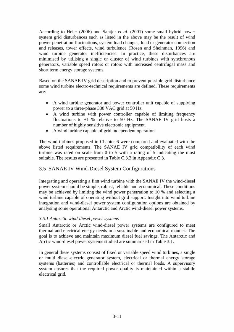
3-11
According to Heier (2006) and Santjer et al. (2001) some small hybrid power system grid disturbances such as listed in the above may be the result of wind power penetration fluctuations, system load changes, load or generator connection and releases, tower effects, wind turbulence (Rosen and Sheinman, 1996) and wind turbine generator inefficiencies. In practice, these disturbances are minimised by utilising a single or cluster of wind turbines with synchronous generators, variable speed rotors or rotors with increased centrifugal mass and short term energy storage systems. Based on the SANAE IV grid description and to prevent possible grid disturbance some wind turbine electro-technical requirements are defined. These requirements are:
A wind turbine generator and power controller unit capable of supplying power to a three-phase 380 VAC grid at 50 Hz.
A wind turbine with power controller capable of limiting frequency fluctuations to ±1 % relative to 50 Hz. The SANAE IV grid hosts a number of highly sensitive electronic equipment.
A wind turbine capable of grid independent operation.
The wind turbines proposed in Chapter 6 were compared and evaluated with the above listed requirements. The SANAE IV grid compatibility of each wind turbine was rated on scale from 0 to 5 with a rating of 5 indicating the most suitable. The results are presented in Table C.3.3 in Appendix C.3.
3.5 SANAE IV Wind-Diesel System Configurations Integrating and operating a first wind turbine with the SANAE IV the wind-diesel power system should be simple, robust, reliable and economical. These conditions may be achieved by limiting the wind power penetration to 10 % and selecting a wind turbine capable of operating without grid support. Insight into wind turbine integration and wind-diesel power system configuration options are obtained by analysing some operational Antarctic and Arctic wind-diesel power systems.
3.5.1 Antarctic wind-diesel power systems
Small Antarctic or Arctic wind-diesel power systems are configured to meet thermal and electrical energy needs in a sustainable and economical manner. The goal is to achieve and maintain maximum diesel fuel savings. The Antarctic and Arctic wind-diesel power systems studied are summarised in Table 3.1. In general these systems consist of fixed or variable speed wind turbines, a single or multi diesel-electric generator system, electrical or thermal energy storage systems (batteries) and controllable electrical or thermal loads. A supervisory system ensures that the required power quality is maintained within a stabile electrical grid.

3-12
Table 3.1 indicates that the common wind turbines of choice are those utilising stall controlled rotors and grid or permanently excited synchronous generators. In these power systems the surplus electrical energy is either stored in battery banks or spent through thermal systems such as snow smelters or electric boilers. Table 3.1: Operational Antarctic and Arctic wind-diesel power systems
Wind-diesel power system [Country]
Win
d t
urb
ine
[t
ype,
cap
acit
y]
Rot
or c
ontr
ol
Gen
erat
or t
ype
Ave
rage
pen
etra
tion
ra
tio
[An
nu
al e
ner
gy
dem
and
in M
Wh
e]
Su
rplu
s el
ectr
ical
en
ergy
man
agem
ent
Princess Elizabeth¥ [Belgium] Rodrigo et al. (2006)
Proven [HAWT, 6 kW]
Stall Permanently excited synchronous
90 % [395]
Storage: batteries, fly-wheel
Casey [Australian] Brown et al. (1996)
Vergnet GEV7.10 [HAWT, 10 kW]
Stall Asynchronous < 8 % [1 720]
Load regulation
Mawson [Australian] Magill et al. (2000) and AAD (2000)
Enercon [HAWT, 280 kW]
Pitch Separately excited synchronous
60 % [2 270]
Storage: Thermally stored
Neumayer II [German] El Naggar (2000)
Heidelberg Motor [VAWT, 20 kW]
Stall Permanent excited synchronous
6 % [630]
None
WASA¥ [Sweden] Henryson and Svensson (2004)
Northern Power Systems [HAWT, 3 kW]
Stall Permanent excited synchronous
97 % [8.760]
Storage: batteries, Dump load: Snow smelter
Wales, Alaska, Drouilhet and Shirazi (2002)
AOC 15/50 [HAWT, 65 kW]
Stall Asynchronous > 50 % [657]
Storage: Batteries Dump load: Electric boiler
¥ Wind-diesel power system performances based on estimations

3-13
3.5.2 The SANAE IV wind-diesel power system configurations proposed
As a first approach the proposed wind-diesel power system will consists of three diesel-generators (i.e. a master, a slave and back-up) and a single small wind turbine. No short term energy storage will be required due to;
the adequate size of an available dump load i.e. 90 kWrated snow smelter) the low initial average wind power penetration (below 10 % or 20 kWrated) the available back-up diesel-electric generator the associated additional capital investment
Wind-diesel power system configuration and its complexity depend on the type of wind turbine generator and the targeted wind power penetration. According to Wildi (2002) and Gasch and Twele (2002) the wind turbine generator types are divided into synchronous and asynchronous generators. Grid or self excited synchronous generators can be operated in both the capacitive and inductive modes and are therefore capable of grid independent operation. Most small wind turbine designs consist of permanently excited synchronous generators with generally directly coupled wind turbine rotors (direct drive). Thus no intermediate gearboxes are required. These wind turbines are most widely utilised in stand-alone wind-diesel power systems. An asynchronous generator is basically an induction machine which operates as a generator once its rotor rotational speed exceeds its stator synchronous speed. The stator synchronous speed depends on the grid frequency which implies that the rotor speed is limited. To integrate such a generator with a fixed frequency grid a constant rotor rotational speed must be maintained. These generators are generally cheaper than synchronous generators although the additional gearboxes and complex rotor speed controls make them unpopular in small wind turbine designs. Wind turbines that utilise induction generators are mostly found in medium to large utility scale wind turbine designs. The SANAE IV wind-diesel power system configuration options are illustratively summarised in Table 3.2. These configurations were grouped in low, medium and high average wind power penetration categories. These options only provide concepts for further detailed grid modification or design which are to be performed by an electrical engineer. In Table 3.2, block 1 and 4 present wind-diesel power systems with low average wind power penetration ratios. In these systems the SANAE IV electrical and thermal energy demands are met by one continuously running diesel-electric generator (master), a backup generator (slave) and small wind turbine. The backup generator operation cycles are partly governed by the intermittent wind power produced. All wind power produced will be supplied to the SANAE IV grid via inventers (synchronous) or converters (induction) systems. No short term energy storage or additional load control systems are required. The first SANAE IV wind-diesel power system may be configured as in block 1.
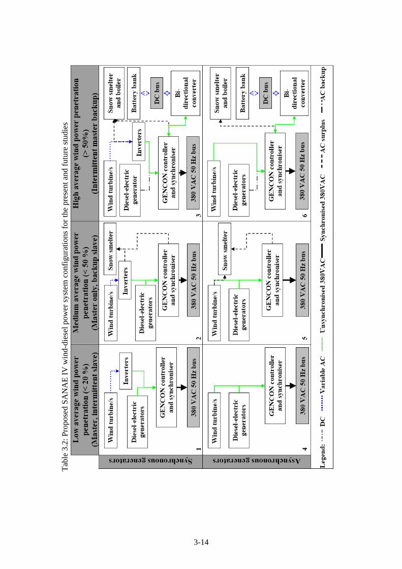
3-14
Tab
le 3
.2: P
ropo
sed
SA
NA
E I
V w
ind-
dies
el p
ower
sys
tem
con
figu
rati
ons
for
the
pres
ent a
nd f
utur
e st
udie
s

3-15
In the near future the SANAE IV wind-diesel power system may expand to a wind-diesel system capable of handling medium to high wind power penetrations. These systems may be configured as shown in blocks 2, 3, 5 and 6. In these systems a single master diesel-electric generator is utilised as either a complimentary or backup power supply. Most of the SANAE IV electrical energy demand will be met by wind power, while excess power may be stored with an energy storage system or diverted to a dump load, e.g. the snow smelter. In a high wind power penetration power system the lack of thermal energy previously recovered from diesel-electric generators must be supplied by other thermal energy systems e.g. electric boiler. The complexity of these systems may entail the replacement of the existing SANAE IV power control system.
3.6 Control Strategy This section presents the conceptual operation modes that may be applied to the SANAE IV wind-diesel power system as proposed in Table 3.2, block 1. The detailed control system design or existing control system modifications are to be performed by an electrical or control system engineer. The first SANAE IV wind-diesel power system will consist of a small wind turbine (less than 20 kWrated) and the existing multi diesel-electric generator system. The wind-diesel power system operation modes are functions of the electrical energy demand and the wind turbine operational wind speed range. SANAE IV wind-diesel operation modes are presented in Figure 3.8.
Figure 3.8: Wind-diesel power system operation modes

3-16
Figure 3.8 explains that the SANAE IV power demand will be supplied by a single diesel-electric generator while the station power demand is below 140 kWe and hub height wind speed below the wind turbine cut-in wind speed. Intermittent wind power is supplied to the station once the wind speed exceeds the wind turbine cut-in wind speed. Thus the station energy demand is met by the wind-diesel system. Similar system operation conditions are expected for a station load below 162 kWe and wind conditions within the wind turbine operational range. If the power demand increases to above 162 kWe and is not met by a single diesel-electric generator and wind turbine, the back-up generator will be switched on. Such a scenario is most likely to occur during the summer season when wind conditions are less favourable and the power demand is increased due to the increased base activities. The SANAE IV wind-diesel power system control system should be designed to ensure maximum wind power utilisation while sustaining optimal diesel-electric generator operation and the described SANAE IV power quality.
3.7 Summary This chapter presented the SANAE IV five part operating system and its associated normal year thermal and electrical energy demands. These demands are met by the current multi diesel-electric generator system. This system annually converts about 300 000 L/a of SAB diesel fuel to 1 024 MWhe/a of electrical energy. The annually thermal energy was estimated at 1 100 MWhth/a. Avoidable impacts of wind power penetration on the SANAE IV diesel-electrical generator system operation were investigated. The severity of these impacts and the complexity of the envisaged SANAE IV wind-diesel system will depend on the wind power penetration and the wind turbine electrical design. Integrating and operating a wind turbine within the envisaged SANAE IV wind-diesel power system should be simple, robust, reliable and economical. It may be achieved by selecting a small wind turbine with a capacity of less than 20 kWrated, a stall controlled rotor and a permanently excited synchronous generator. Some electro-technical criteria derived from the SANAE IV energy demand analyses and grid assessment results were presented. The criteria were applied in the evaluation of the small wind turbines proposed in Chapter 6. As a result the most electro-technical compatible wind turbines were identified, namely the Proven 6 kWrated, Bergey 10 kWrated and Fortis 10 kWrated wind turbines.

4-1
CHAPTER 4 WIND TURBINE MICRO-SITING This chapter presents the climatological, environmental and technical related Vesleskarvet site assessments performed. The results are applied in the evaluation of possible Vesleskarvet wind turbine sites. The identified sites, as a first estimate, may be considered suitable for the deployment of a single or, in near future, a cluster of small wind turbines. Section 4.1 presents the results of the climatological related site assessment performed. The optimal site specification is based on the numerically generated Vesleskarvet wind resource map and the local climate assessment results presented in Chapter 2. Vesleskarvet specific environmental issues such as the definition of protected scientific research areas and biospheres, wind turbine noise and visual impacts are addressed in Section 4.2. Section 4.3 describes technical related siting issues such as electrical grid connection constraints, site accessibility, electro-magnetic interference and aviation interference. The most suited Vesleskarvet wind turbine sites are specified in Section 4.4.
4.1 Site Selection based on Climatic Conditions The climatologically specific wind turbine site evaluation involves three factors, namely wind speed, wind turbulence and sastrugi formation. Both wind speed and turbulence governs wind turbine yield, operational availability and operational safety. Turbulence induced by the wind turbine may also impact the integrity of near downstream structures. Wind turbine induced sastrugi may complicate system maintenance and obstruct some SANAE IV operations. The numerically generated Vesleskarvet 10 m AGL spatial wind speed distribution is presented in Figure 4.1. This distribution shows the localised flow separation and recirculation zones which are confined to the SANAE IV base, SHARE antennae and fuel bunker structures. These flow conditions are also shown in the associated spatial turbulence intensity distribution which is presented in Figure D.4.1 in Appendix D.4.1. Figure 4.2 presents an estimated wind power density distribution. Wind power densities of above 2000 W/m2 for areas located upwind between the SANAE IV base and fuel bunkers may be expected. Eight wind turbine sites as indicated in Figures 4.1 and 4.2 were selected. Sites with height specific wind speed above 11 m/s, estimated wind turbulence intensity below 10 % and the wind power density above 2 000 W/m2 are selected. These wind speed and turbulence intensity values relate to the lowest hub height rated wind speed and turbulence conditions as specified for the wind turbines proposed in Chapter 6. The first five sites are located along the snow-rocky Vesleskarvet cliff edge. The last three sites are located in the snow/ice region just upstream of the SANAE IV base.
4-2
Fig
ure
4.1
: Ves
lesk
arve
t spa
tial
win
d sp
eed
dist
ribu
tion
at a
hei
ght o
f 10
m A
GL
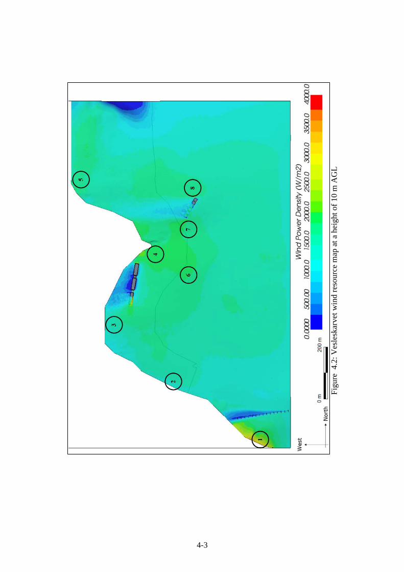
4-3
Fig
ure
4.2
: Ves
lesk
arve
t win
d re
sour
ce m
ap a
t a h
eigh
t of
10 m
AG
L

4-4
Snow build-up created by a wind turbine at these selected sites may have minimal impact on the current SANAE IV base activities. In fact snow build-up induced by a wind turbine can be beneficial. A wind turbine placed at site 6 may increase the availability of snow which is to be melted at the nearby snow smelter. Such snow availability may advance the time intensive snow smelter filling sessions. The change in wind speed, turbulence intensity and wind power density with height at these proposed sites are investigated. Normalised vertical wind speed profiles associated with the selected sites are derived from the CFD results. These non-standard profiles as compared in Figure 4.3 are also comparable to profiles obtained by Lun et al. (2003). Wind speed, turbulence intensity and wind power density distributions calculated for heights of 18 m and 36 m AGL are presented in Figures CD.3.1 to CD.3.6 in Appendix CD.3.1. These heights relate to the standard hub heights of wind turbines described in Chapter 6.
0.85 0.9 0.95 1 1.05 1.1 1.15 1.2 1.25 1.30
5
10
15
20
25
30
35
40
45
50
55
Wind speed normalised with 12 m/s
He
igh
t A
GL
[m
]
Site 1 Site 2 Site 3 Site 4 Site 5 Site 6 Site 7 Site 8
Figure 4.3: Normalised site specific wind speed profiles
4.2 Environmental Impact Assessment This section describes the exclusive Vesleskarvet micro research reserves and presents the potential wind turbine related visual and noise disruptions. These assessments were based on case studies found in literature.
4.2.1 Exclusive micro research reserves
The Vesleskarvet micro research areas may be divided in to three primary disciplines, namely the geoscience, space science and bioscience research areas. Detail on the on going research conducted within these areas is described by SANAP (2008). The space science research zones as specified in Figure 4.4 comprise a magnetic quiet zone, the SHARE antennae zone and the VLF antennae zone. Deploying a wind turbine in the vicinity of these zones is strictly prohibited.

4-5
The northern Vesleskarvet buttress is the habitat of some lichen and mite (Maudheimia) species (Anonymous, 2001). In Figure 4.4, most of the northern buttress is a declared biological and geological research reserve.
4.2.2 Visual impact assessment
Wind turbine or wind farm visual impact assessment methodologies as outlined by Manwell et al. (2003), Möller (2006) and Stanton (1994), concerns analysing the impact of a structure on the surrounding natural landscape by determining the severity of view disruptions caused by deviation in form, line, colour and texture. As a first approach wind turbine shadow casting and possible viewshed (existing unspoiled visual setting) alteration relevant to the Vesleskarvet landscape and SANAE IV base were assessed. Daytime wind turbine shadow casting both static and dynamic (flicker) is limited to the summer season. Shadow casting on the SANAE IV base may be minimised by placing the wind turbine at a distance of eight rotor diameters (8Drotor) measured from the base perimeter. During the winter the wind turbine silhouette, if located in close proximity to the base may degrade Aurora Australis observations and affect studies. The SANAE IV base is situated on Vesleskarvet, a nunatak which ramps to about 200 m above the surrounding ice shelf. The topography provides the base with an unprecedented view of the pristine snow covered surrounding mountain ranges, nunataks and glaciers. Lorenzenpiggen, a mountain peak located approximately 9 km due south of SANAE IV, is probably the most photographed mountain peak within the region. Some viewsheds as observed from the base are presented in Figures D.4.1 and D.4.2, Appendix D.4.2. With reference to Chapter 2, in summer viewing a black rotor at a height of 10 m AGL against the white Antarctic scenery will disrupt that specific viewshed. The expected visual disruption experience may be identical to a disruption experienced when studying Figure D.2.3 (Crane, 2008), Appendix D.2. Erecting a wind turbine within existing spoiled viewsheds as specified in Figure 4.4 are preferred.
4.2.3 Wind turbine noise emission
Wind turbine noise may be divided into source specific mechanical noise and aerodynamic noise sources. Mechanical noise sources are gearboxes, yaw drives and the generator. Aerodynamic noise is in fact audible turbulence caused by flow separation from blades, tower and nacelle. In cold climates, wind turbine aerodynamic related noise variations may be used to detect blade icing. The noise levels of some wind turbines proposed in Chapter 6 are listed in Table D.3.1, Appendix D.3. These noise levels were specified by Anonymous (2008b) and Bergey (2007). Noise levels of the Vergnet wind turbines were estimated by means of models specified by Wagner et al. (1996) and Rogers et al. (2006). As a result all wind turbines, except the Fuhrländer wind turbine, may emit noise of below 70 dB(A) observed at a relative distance of 20 m.

4-6
Fig
ure
4.4:
Res
ults
of
the
Ves
lesk
arve
t vis
ual i
mpa
ct a
sses
smen
t.

4-7
4.3 Technical Site Survey This survey assesses the Vesleskarvet site to determine the potential technical wind turbine installation, operation and decommissioning issues which may disrupt the current SANAE IV base activities.
4.3.1 Installation and decommissioning issues
Wind turbine installation or decommissioning site specific surveys entail the assessment of physical and temporal site accessibility, site preparation, wind turbine foundation designs and grid connection options. During the annual summer takeover period most SANAE IV containerised cargo is transport along one of two possible routes. These routes are mapped in Figure D.4.1, Appendix D.4.1. Route accessibility and usage depends on the sea-ice surrounding the continent. Sensitive scientific equipment is flown via helicopter. Vesleskarvet routes suitable for the transportation of cargo like wind turbines are specified in Figure D.4.2 in Appendix D.4. The SANAE IV wind turbine foundation design and construction depends on the proposed site orography. At SANAE IV the construction of concrete foundations are prohibited. Some of the foundation types most commonly constructed in Antarctic are the rock anchored pylon or submerged snow-ice foundation types. These foundation types are further described in Appendix D.4.1. The potential areas assumed suitable for the construction of such foundations are specified in Figure D.4.2 in Appendix D.4. Some foundation designs and construction methods as described by Petrie et al. (2007) are included in Appendix CD.3. Site preparation periods, preparation equipment required, geotechnical investigations and costs depend on the wind turbine and site selected. Only two power transmission lines exist at Vesleskarvet. Like at most Antarctic stations these transmission lines are suspended at approximately 2 m AGL to ensure that these lines remain ice-free and accessible. One transmission line links the SANAE IV base with the snow smelter, while the second supplies power to the fuel bunker pump station. The same electric cabling used to supply power to the 90 kWrated snow smelter should be used to connect the proposed wind turbine to the SANAE IV grid. Constructing a new power transmission line is seen as an unnecessary capital expense but if the proposed wind turbine is sited close to the existing power transmission lines, further capital savings are possible. The SHARE antennae array is linked to SANAE IV via a buried communication line routed within an irrigation pipe conduit. This conduit may also be used to house a power transmission line. The above transmission and conduit layouts are specified in Figure 4.5.

4-8
Fig
ure
4.5:
Ves
lesk
arve
t pow
er tr
ansm
issi
on a
nd c
omm
unic
atio
n li
ne la
yout
s

4-9
4.3.2 Potential operational issues
This section describes the potential aviation, Electro-Magnetic Interference (EMI) and Radio Frequency Interferences (RFI) caused by the proposed wind turbine. Wind turbine related safety hazards such as ice shedding (Chapter 2) and blade throw are also addressed. The SANAE IV base provides and acts as an emergency and rescue base to its neighbouring Norwegian and German stations. Occasional air traffic between SANAE IV and its neighbours is expected. Furthermore, during the summer visitors and cargo are flown in by helicopter. These helicopter flight operations are mostly confined to the flight deck which form part of the SANAE IV base. Areas relevant to aviation operations such the landing strip and helicopter flight deck are specified in Figures 4.5 and D.2.1 in Appendix D.2. Erecting wind turbines within these areas are not recommended. Flow conditions induced by aircraft active within these areas may cause premature wind turbine failure. The possible icing and high wind conditions at Vesleskarvet are described in Chapter 2. These conditions may pose safety hazards such as ice shedding and blade or tower failures. Ice shedding from the nacelles and blades of the wind turbines proposed in Chapter 6 are theoretically investigated. Ice shedding safe distance from the wind turbine is estimated by means of empirical ice shedding prediction models described by Seifert et al. (2003). Wind turbine blade failure may result from blade material imperfections which are amplified by low temperature conditions, unbalanced loading caused by blade icing, faulty rotor speed control, etc. Potential wind turbine blade throw safe distances are estimated by means of theoretical blade or blade fragment throw prediction methods described by Turner (1989) and Mocilla (2006). Blade throw and ice shedding related calculations are presented in Appendix D.5. The estimated maximum ice shedding and blade throw safe distances are 50 m and 312 m respectively. A detail analysis of potential electromagnetic interference caused by the wind turbines proposed in Chapter 6 is not performed, expected interferences are described. Manwell et al. (2003) and Wagner et al. (1996) discussed typical wind turbine related electromagnetic interference effects. A wind turbine excites magnetic and electrical fields and if placed between a radio, television or microwave transmitter and receiver it may alter or reflect the electromagnetic signal. The degree of signal distortion typically depends on the wind turbine topology, rotor rotational speed, blade construction and its material and tower geometry. Older wind turbines had full or partial metal blades which caused electromagnetic interference. Nowadays, wind turbines have composite blades which are less likely to produce electromagnetic interference, although some with blade lighting protection (i.e. a conductor situated on blade surface) may cause electromagnetic interference.

4-10
The wind turbines proposed in Chapter 6 have composite blades and simple tubular steel towers. Glass fibre epoxy blades are partially transparent to radio waves. The size of these wind turbines may only degrade UHF and microwave signals.
4.4 Summary This chapter presented climatological, environmental and technical wind turbine siting related issues. Eight potential wind turbine sites were identified from the CFD simulation results. With reference to the environmental and technical requirements described the number of potential sites is limited to three. The sites marked 4, 7 and 8 as shown in Figure 4.1 are suggested. The identified sites, as a first estimate, may be considered suitable for the deployment of a single or, in near future, a cluster of small wind turbines. The reasons for the selection of these three sites include:
the estimated favourable wind conditions these locations are outside areas reserved for scientific research these sites are located within an already spoiled view sector these locations are in the vicinity of the existing power transmission lines the site is accessible via existing routes these locations are outside the expected flight zones the distance between these locations and the base may result in no ice
shedding and blade throw related incidents or damage These sites are located within a snow-rocky area. Therefore a rock anchored pylon wind turbine foundation should be designed and constructed. Note that both sites marked 7 and 8 are located close to the fuel bunker structure. Mounting the proposed wind turbine on the eastern side of the fuel bunker may be another feasible possibility. Such a wind turbine integration may eliminate the need for the additional foundation and power line design and construction. However, the impact on the bunker structure integrity with the integration of a wind turbine needs to be investigated. Ultimately, if such a notion is implemented cost saving may be expected.

5-1
CHAPTER 5 WIND-DIESEL SYSTEM ECONOMY In specifying a wind turbine which is to be integrated with the current SANAE IV diesel-electric generator system, the associated technical and economical feasibilities should be investigated. Economic feasibility relates to costs avoided as a result of power produced by the wind turbine. In this study avoided costs are limited to diesel fuel savings, diesel-electric generator operation and maintenance savings and externalities. This chapter starts with Section 5.1 which summarises the SANAE IV wind turbine life cycle expenditures. Section 5.2 presents the recurring wind-diesel power system costs and savings. Next, Section 5.3 represents some of the wind-diesel system economic assessment methodologies found in literature. Sections 5.4 and 5.5 present the results of the SANAE IV wind-diesel economic assessments and economic sensitivity analyses performed. Lastly, Section 5.6 summarises all of the above.
5.1 Wind Turbine Life Cycle Investment Costs The SANAE IV wind turbine life cycle costs are numerous. Teetz (2002), Olivier (2006) and Hunter and Elliot (2005) classified these costs based on the relevant wind power development phases. These costs are represented below: Feasibility study:
wind resource assessment technical site survey electro-technical grid evaluation wind turbines available project design and management project approval and permits
Wind turbine and equipment:
wind turbine and control system cold climate modification and testing spare parts and tools grid connection equipment and switchgear wind turbine importation and temporary storage
Engineering:
site design e.g. access roads, necessary infrastructure mechanical system design e.g. foundation, tower electrical system design e.g. grid connection, power conditioning
and management, etc.

5-2
Balance of plant: wind turbine packaging and transportation to Antarctica and from
ship to site site preparation wind turbine erection grid connection system mechanical and electrical testing commissioning of system
Operation:
wind turbine monitoring operation and maintenance (O&M) grid connection and power production monitoring
Decommissioning:
grid disconnection wind turbine dismantling packaging and transportation from site to ship and via ship to
South Africa removal of excess infrastructure and site rehabilitation
Miscellaneous: training overwintering technicians administration and contingencies
5.2 Annual Wind-Diesel System Costs and Savings The implementation and integration of a wind turbine with the current SANAE IV diesel-electric power system will create additional annual recurring costs and savings. The life cycle economic feasibility of the SANAE IV wind-diesel system depends on cost-to-saving ratios. Costs and savings accounted in the SANAE IV wind-diesel economic assessment are:
Wind-diesel O&M costs Diesel fuel savings due to the power produced by wind turbine Diesel-electric generator O&M savings due to the reduced use External savings due to the reduced fuel spillages and reduced emissions
5.2.1 Wind-diesel O&M costs
The O&M cost of a small wind turbine operational within a remote power wind-diesel power system may vary between 3 % and 8 % of the initial investment capital per year (Manwell et al., 2003). Devine et al. (2004) reported O&M costs of 3 % of the investment cost for an Alaskan wind-diesel power system.

5-3
The remoteness of the SANAE IV base led to the implementation of a pro-active base maintenance plan. This means that all necessary parts, lubricants and maintenance tools are ordered and stored on site. The proposed SANAE IV wind-diesel system O&M costs comprise the labour, wind turbine and diesel engine components, component management and storage, mechanical and electrical scheduled and unscheduled maintenance, manual de-icing related costs. Typical annual wind turbine O&M costs may vary around 5 % of the purchase price (Spera, 1994), while diesel-electric generator O&M costs amount to approximately 8 % of the fuel price (Hunter and Elliot, 2005). Thus the SANAE IV diesel-electric generator system O&M cost was estimated at 0.51 ZAR/L of diesel fuel consumed. An O&M cost escalation rate of 2 % for both wind turbine and diesel-electrical systems is assumed. Olivier (2006) estimated that the price of diesel fuel at SANAE IV is approximately three times the price of fuel in Cape Town, South Africa. Accordingly to DEAT (2008) the subsidised purchase price of SAB diesel fuel is 6.34 ZAR/L. Therefore, at the time of study, the price of diesel at SANAE IV is 20.92 ZAR/L. The price of diesel fuel is governed by inflation fluctuations in the South African economy and the international crude oil price. It is therefore difficult to predict future fuel prices and escalation rates. A diesel fuel escalation rate of 2 % was assumed. The assumption was based on historic South African fuel prices (Sasol, 2008).
5.2.2 Diesel fuel and O&M cost savings
The SANAE IV annual diesel fuel savings are depending on the diesel fuel price, fuel price escalation rate and wind power penetration ratio. As in Chapter 3, the integration of a small wind turbine with the current SANAE IV power system will impact on the operation of the slave diesel-electric generator. Without the necessary power system modification, the fuel and O&M savings may be limited. The SANAE IV annual diesel fuel savings are approximated with Equation 3.1 (see Section 3.2.1) and the theoretical wind turbine yields as calculated in Section 2.6. Diesel-electric generator system O&M savings are estimated on the basis of conditions defined in the above.
5.2.3 Externalities
An external cost is created when the social and economic activities of one group has an unaccounted impact on the social and economic activities of another group (Busquin, 2003). In the Antarctic context, the impact of fossil fuelled power system emissions has an unaccounted impact on the pristine Antarctic research environment. Reducing fossil fuel usage in Antarctica may yield environmental and future economic benefits. Utilising wind power at SANAE IV will reduce the current green house gas emissions and fuel spillages. If Antarctic stations are allowed to trade international CO2 credits the installation of renewable energy systems may be funded by the generated capital.

5-4
Taylor et al. (2002) and Olivier (2006) estimated the annual tonnages of SANAE IV diesel-electric power system emissions. Based on this, pollutant specific billing was estimated. Emission tonnage and total pollutant specific billing estimates are represented in Tables 5.1 and 5.2 respectively. Table 5.1: SANAE IV total annual emissions (Taylor et al., 2002)
Estimated annual tonnage [t/a]
VOC CO NOx SO2 CO2 PM
Lower 0.34 0.53 13.45 0.08 744 0.2
Upper 0.55 0.85 13.45 0.08 744 0.3 Table 5.2: Pollutant specific costs (Olivier, 2006) Pollutant Pollutant specific billing [ZAR/kg] Annual cost [ZAR/a]
CO 41.59 35 352.50
CO2 0.20 148 800.00
NOx 25.40 341 630.00
PM 36.62 11 718.40
SO2 62.76 5 020.80
VOC 41.59 22 875.50
Total cost: 565 395.20 In Table 5.2 the annual external cost based on listed pollutants amounts to 565 395 ZAR/a which is equivalent to 2.27 ZAR/L of diesel fuel consumed. The total external cost includes the environmental damage caused by emissions and fuel spillages. Costs related to fuel spillages further include the labour and processing costs of fuel spill clean-ups. Olivier (2006) stated that the external cost associated with fuel spillage is approximately 290 % higher than emission based externalities. Therefore the fuel based total annual external cost amounts to 6.59 ZAR/L of fuel consumed by the SANAE IV diesel-electric power system.
5.3 Wind-Diesel Economic Assessment Methodologies In this study, detailed economic assessment methods that include the time value of money in the calculation of life cycle economic performance parameters are used (Manwell et al., 2003; Hunter and Elliot, 2005). The detailed economic parameters calculated in this study are represented below.
5.3.1 Net Present Value (NPV)
As part of a life cycle economic assessment, the NPV of costs or savings estimate the Present Value (PV) of future costs or savings. NPV is estimated by the summation of the yearly PV inflated and discounted costs. The inflated PV and NPV of the SANAE IV wind-diesel system costs and savings are estimated by means of Equations 5.1 and 5.2 respectively.

5-5
1 1 1 1 1(1 ) (1 ) (1 ) (1 ) (1 )
(1 ) (1 ) (1 ) (1 ) (1 )
j j j j j
j j j j j j
i LCC i TC i OM i F i XPV
r r r r r
5.1
1
N
jj
NPV PV
5.2
Where LCC is the life cycle cost, which is the summed present worth of the total capital (TC), operation and maintenance (OM), diesel fuel (F) and external (X) costs in the South African Rand [ZAR]. The interest rate (r) and inflation rate (i) are fractions, j is the year relative to the investment year and N the investment period. In this study an investment period of 20 years was assumed.
5.3.2 Internal Rate of Return (IRR)
The IRR is a measure of investment profitability. An IRR above the general interest rate is indicative of a profitable investment. IRR is the calculated interest rate for a NPV of savings equal to zero as specified in Equation 5.3.
1
1
(1 )( ) 0
(1 )
jN
jj
iLCS LCC
IRR
5.3
Where LCC and LCS are the respectively life cycle cost and life cycle saving in ZAR, IRR the internal rate of return as a fraction, i the inflation rate as a fraction, j the year relative to investment year and N the investment.
5.3.3 Cost of Energy (COE)
The cost of energy is calculated by dividing the summed life cycle costs by the total amount of energy produced over the same life time. Equation 5.4 represents the definition of the COE:
N
N
LCCCOE
E
5.4
where COE is the cost of energy in [ZAR/kWhe], LCC is the life cycle cost in [ZAR], E the electrical energy in [kWhe] and N the investment period.
5.3.4 Economic sensitivity analysis
The accuracy of a life cycle economic assessment depends on the accuracy of the predicted time dependent variables such as the interest and inflation rates. Economic risks relevant to the capital investment are estimated by means of an economic sensitivity analysis, which concerns the calculation of the economic performance parameter (e.g. COE) deviation relative to its current value by varying a single time dependent economic variable (e.g. interest rate).

5-6
5.4 Wind-Diesel Economic Assessment Economic assessments of the eight wind turbines considered in Chapter 6 are performed. Assessments are based on the wind turbine, SANAE IV diesel-electric system and general economic assumptions (SARB, 2008) listed in Tables E.1.1 and E.2.1. Assumptions are based on assessments performed by Hunter and Elliot (2005), Frye (2006) and McKenna and Olsen (1991). The economic feasibility of each wind-diesel system is determined by comparing the calculated NPV, IRR and COE of each of the wind-diesel systems to the relevant economic parameters calculated for the current diesel-electric generator system. A sample calculation which presents the Proven6 wind-diesel system assessment is included in Appendix E.2.
5.4.1 Net Present Values
The inflated NPV of costs incurred by the current SANAE IV diesel-electric generator system is compared to that of the Proven6 and Fuhrländer30 wind-diesel systems (Figure 5.1) using Equations 5.1 and 5.2. Associated external costs are excluded.
0 2 4 6 8 10 12 14 16 18 20-90
-80
-70
-60
-50
-40
-30
-20
-10
0
10
Wind-diesel system lifetime [Years]
NP
V o
f C
os
ts [
mill
ion
ZA
R]
SANAE IV diesel-electric generator system Proven6 wind-diesel system Fuhrländer30 wind-diesel system
Figure 5.1: NPV of costs incurred during project lifetime
Both the Proven6 and Fuhrländer30 wind-diesel systems reach costs less than of the diesel-electric generator system within two years (Figure 5.1). Reasons for the short redemption periods are the high point-of-use diesel price and high inflation rate. The inflated NPV of lifetime savings of both the Proven6 and Fuhrlander30 wind-diesel power systems are presented in Figure 5.2. Note that the associated external savings of both wind-diesel systems are almost negligible. Savings earned by these wind-diesel systems primarily depend on the amount of fuel saved.

5-7
0 2 4 6 8 10 12 14 16 18 20-2
0
2
4
6
8
10
12
14
16
18
Wind-diesel system lifetime [Years]
NP
V o
f S
av
ing
s [
mill
ion
ZA
R]
Proven6 wind-diesel system Proven6 wind-diesel system (externalities) Fuhrländer30 wind-diesel system Fuhrländer30 wind-diesel system (externalities)
Figure 5.2: NPV of savings with external costs included
5.4.2 Internal Rate of Return
The IRR of the Proven6 and Fuhrländer30 wind-diesel systems are calculated by means of Equation 5.3. The calculated IRR variation associated the capital investments in the two wind-diesel systems are presented in Figure 5.3. Note that the Proven 6 wind-diesel system has an IRR of 54 %. When compared to the general interest rate of 15 % it is evident that the associated capital investment is desirable.
-3.0-2.5-2.0-1.5-1.0-0.500
20
40
60
80
100
120
Total capital investment [million ZAR]
IRR
[%
]
Proven6 wind-diesel system Fuhrländer30 wind-diesel system
Figure 5.3: Comparison of the IRR values

5-8
5.4.3 Cost of electrical energy
The cost of electrical energy produced by the SANAE IV diesel-electric generator system is compared to the energy production costs of the Proven6 and Fuhrlander30 wind-diesel systems (Figure 5.4). These energy production costs were calculated by means of Equation 5.4. Externalities earned due to the wind power were not incorporated in these calculations.
-4.0-3.5-3.0-2.5-2.0-1.5-1.0-0.55
5.5
6
6.5
7
7.5
8
Total capital investment [million ZAR]
CO
E [
ZA
R/k
Wh e
]
Diesel-electric generator system Proven6 wind-diesel system Fuhrländer30 wind-diesel system
Figure 5.4: Electrical energy conversion costs
Figure 5.4 presents the energy production costs of different total capital investments. The SANAE IV diesel-electric generator and Proven6 wind-diesel systems have energy production costs of 6.82 ZAR/kWhe and 6.58 ZAR/kWhe respectively, indicating a saving in energy production cost of approximately 4 %. Teetz (2002) estimated that a SANAE IV wind-diesel with a 100 kW wind turbine would reduce the energy production cost by 20 %.
5.4.4 Economic evaluation of the wind-diesel systems
The SANAE IV wind turbine is selected on the basis of its technical and economical feasibility. Results of the environmental and electrical technical feasibility assessments are discussed in Chapters 2 and 3. Results of the economic assessments performed are presented in this section. The NPV of cost and savings, IRR, COE and simple payback periods of each wind-diesel system considered for the SANAE IV wind-diesel system were calculated. The eight wind-diesel system options are compared based on these results; see Table E.3.1, Appendix E.3. These wind-diesel systems are rated on a scale from 0 to 5, with 5 meaning a desirable investment and 0 meaning a less attractive investment.

5-9
Of the eight wind-diesel systems evaluated, Proven6, Vergnet10 and Fuhrländer30 wind-diesel systems are the most attractive investment options (Table E.3.1). The Proven6 wind-diesel system has a NPV of savings which is comparable to the savings of the Fortis10 wind-diesel system. It implies that the small investment associated with the Proven6 wind-diesel system outperform the investment related to Fortis10 wind-diesel system. In the 10 kW wind turbine class (i.e. Bergey, Fotris and Vergnet wind turbines) the Vergnet10 wind-diesel system has the lowest electrical energy production cost. Based on the assumptions listed in Tables E.1.1 and E.2.1 the Fuhrlander30 wind-diesel system is the most economically feasible system of all those considered.
5.5 Economic Sensitivity Analyses All the economic performance parameters calculated in the assessments are based on the May 2008 inflation, interest and escalation rates and fuel price. Future changes in inflation, interest, currency exchange and escalation rates and fuel price are difficult to predict, therefore the impact of these changes on the economic performance of the Proven6 and Vergnet10 wind-diesel systems are determined by performing sensitivity analyses. Results of the sensitivity analyses performed are presented in Figures 5.5 and E.1., respectively. In Figure 5.5 the Proven6 wind-diesel system NPV of savings deviations are presented. These deviations measured relative to the value given in Table E.2.2 are calculated by varying the fuel escalation rate, wind turbine O&M cost and wind turbine purchase price. Note that a larger diesel fuel price increase will result in a small savings increase.
-100 -80 -60 -40 -20 0 20 40 60 80 100-100
-50
0
50
100
150
200
250
Deviation [%]
NP
V o
f s
av
ing
s d
ev
iati
on
s [
%]
Diesel fuel escalation rate Interest rate General inflation rate Wind turbine purchase price
Figure 5.5: Results of the Proven6 wind-diesel power system economic
sensitivity analysis

5-10
5.6 Summary This chapter presented the results of the economic assessments as well as wind turbine evaluations performed. These assessments were based on the Vesleskarvet wind resource assessment data provided in Chapter 2, the wind turbines proposed in Chapter 6 and the May 2008 South African economy data. All wind turbines considered for the SANAE IV wind-diesel system will recover their associated capital investments within their design lifetime of 20 years. The estimated diesel fuel savings and reduced environmental cost associated with the integration of these wind turbines will increase the SANAE IV base sustainability and minimise its environmental impact. Three of the eight wind turbines considered for the SANAE IV wind-diesel system were chosen on the basis of their estimated economic performances. These are the Proven 6 kW, Vergnet 10 kW and the Fuhrländer 30 kW wind turbines. The economic performances of these wind turbines when integrated with the SANAE IV diesel-electric power system are summarised below. An average cost of energy production associated with the SANAE IV diesel-electric generator system is estimated at 6.82 ZAR/kWhe. The Proven 6 kW wind turbine would yield annual diesel fuel savings of approximately 10 838 L/a which results to a reduced energy production cost of 6.58 ZAR/kWhe. Furthermore, the Proven6 wind-diesel system would arrive at a breakeven point within two years and capitulate a NPV of 2 586 140 ZAR after 20 years. The Vergnet 10 kW wind turbine when integrated with the SANAE IV diesel fuelled power system would reduce the annual base fuel consumption by an estimated 18 964 L/a. This wind-diesel system would reduce the energy production cost by approximately 7 %. The capital investment associated with this wind-diesel system will be recovered within the second year after it has been commissioned. Over its lifetime of 20 years it this wind-diesel system would generate a NPV of 4 597 532 ZAR. The Fuhrlander30 wind-diesel system which utilises the 30 kW Fuhrländer wind turbine would even its capital investment within two years. It is expected that this wind-diesel system would equate to a NPV of approximately 11 978 010 ZAR at the end of its lifetime. The estimated annual diesel fuel savings of 48 373 L/a would result to energy production cost of approximately 5.71 ZAR/kWhe. The wind turbines discussed above would all yield favourable savings and preserve the pristine Antarctic environment.

6-1
CHAPTER 6 SMALL WIND TURBINE MARKET ASSESSMENT AND SELECTION
A European Commission subsidiary namely the Small Wind Industry Implementation Strategy (SWIIS) consortium classifies wind turbines with a rated capacity of less than 100 kW as small wind turbines. The aim of the SWIIS consortium is to promote the utilisation of small wind turbine technologies. The small wind turbines proposed for the SANAE IV base are selected from the SWIIS wind turbine manufacturer database (SWIIS, 2008). In this chapter, Section 6.1 describes the small wind turbine market assessment performed. Section 6.2 presents and describes the eight commercially available small wind turbines proposed for the SANAE IV base. Technical compatibility and economical feasibility evaluation of these eight selected wind turbines are determined as described and presented in Chapters 2, 3 and 5. Results of these evaluations are summarised in Section 6.3. Three of the initial eight wind turbines are proposed for the first SANAE IV wind-diesel power system. The three selected wind turbines are briefly described in Section 6.4. This chapter concludes with Section 6.5 in which the key points are summarised.
6.1 Small Wind Turbine Market Assessment The small wind turbine market assessment concerned the sourcing of local and global well established wind turbine designs manufactured by market matured wind turbine manufacturers. In performing such an analysis the desired level of technical wind turbine support, maintainability and operation availability may be secured. Some specific wind turbine and manufacturer evaluation criteria partially derived from general system engineering design criteria (Blanchard and Fabrycky, 1997) were defined. The criteria address the wind turbine and subsystem supportability, product maturity and cold climate compatibility. Criteria listed below were applied in the evaluation of the 54 wind turbines (SWIIS, 2008): Wind turbine design maturity and cold climate operation
At least 100 wind turbines installed and still in operation Evidence of cold climate survivability Evidence of wind turbines operational in a diesel-electric power system
Wind turbine component availability and supportability
Wind turbine manufacturer in industry for more than 20 years At least more than 3 wind turbines of different capacity on market An South African reseller or installation Customer and project references Lifetime maintenance and service contracts possible

6-2
Wind turbine design quality Evidence of wind turbine and component test and evaluation results Evidence of wind turbine design standard followed or wind turbine
installation certification
Market assessment results are summarised in Table F.1.1 in Appendix F.1. As a result, eight of the 54 wind turbines and related manufacturers listed in the SWIIS database are selected. The technical and economical performances of these eight horizontal axis wind turbines within the first SANAE IV wind-diesel power system are investigated.
6.2 Small Wind Turbine Assessment All eight wind turbines selected for the further technical and economical evaluation are of European or American make, because the current South African small wind turbine industry is still in its infancy. The handful of South African small wind turbine manufacturers which were considered, are listed in Table 6.1. Table 6.1: List of South African small wind turbine manufacturers Manufacturer [website]
Wind turbine [wind turbine topology]
African Windpower [http://www.africanwindpower.com]
2 kWrated
[HAWT] Phieco [http://www.phieco.net/motorpower]
9 Wrated
[HAWT] Kestrel Wind Turbines [http://www.kestrelwind.co.za]
3 kWrated [HAWT]
Turbex Rotary Wind Mills [http://www.turbex.co.za]
5 kWrated [HAWT]
Winglette Wind Machines [http://www.winglette.com]
10 kWrated [HAWT]
The following eight wind turbines are selected:
1. Proven 6 kWrated 2. Bergey 10 kWrated 3. Fortis 10 kWrated 4. Vergnet 10 kWrated 5. Proven 15 kWrated 6. Vergnet 20 kWrated 7. Eoltec 25 kWrated 8. Fuhrländer 30 kWrated
Some technical details of the above listed wind turbines are represented in Table F.1.2 in Appendix F.1. Additional information is included in Appendix CD.4.

6-3
The technical and economical feasibility of selected wind turbines are derived from the number of evaluations as described in Chapters 2, 3 and 5. Cold climate and SANAE IV specific technical and economical performance measures are applied. Each wind turbine is rated on the basis of its technical and economical performance measures. These wind turbine specific ratings are represented in Table 6.2. Table 6.2: Final wind turbine assessment Technical and economical performance categories
Pro
ven
6
kW
rate
d
Ber
gey
10 k
Wra
ted
For
tis
10
kW
rate
d
Ver
gnet
10
kW
rate
d
Pro
ven
15
kW
rate
d
Ver
gnet
20
kW
rate
d
Eol
tec
25 k
Wra
ted
Fu
hrl
änd
er
30 k
Wra
ted
Topology and materials
4 5 4 3 5 3 4 4
Drive train and control
5 4 4 2 5 2 4 2
Operation 5 4 4 3 4 3 3 2 Theoretical performance
5 4 5 4 4 3 4 2
Theoretical wind power penetration
3 3 3 3 2 2 4 2
SANAE IV grid compatibility
4 5 5 3 3 3 4 3
Estimated economic feasibility
5 4 3 5 4 4 3 5
Overall rating [0-35] 31 29 28 23 27 20 26 20 In Table 6.2, the Vergnet 20 kWrated and Fuhrländer 30 kWrated wind turbines scored the lowest overall rating. Both designs utilise asynchronous generators and gearboxes. At Vesleskarvet, the operation of these wind turbines of limited wind speed and temperature operation ranges may not be feasible. The Proven 6 kWrated, Bergey 10 kWrated and Fortis 10 kWrated wind turbines scored the highest overall. These wind turbines are robust in design and have been utilised in some Antarctic regions. The associated manufacturers may be considered as country specific market leaders, therefore a high level of secure after sale technical and component support, upgrades and maintenance security may be expected. Some installation and integration information relevant to the implementation of the Proven 6 kW, Bergey 10 kW and Fortis 10 kW wind turbines are presented in the following section.

6-4
6.3 Wind Turbine Installation and Integration Considerations This section describes the Proven 6 kW, Bergey 10 kW and Fortis 10 kW wind turbines and provides suggestions regarding the purchase, installation and integration thereof. Relevant technical details are included in Appendix CD.4.
6.3.1 The Proven 6 kW wind turbine
This Scottish wind turbine design is simple and robust. At its core is an encapsulated permanent magnet generator which is linked to a free yawing three bladed rotor. The downwind mounted hub utilises a Zebedee hinge system which controls the rotor speed by flexing the blades to accomplish stall. The self-erecting tubular tower (Figure 6.1) is available in lengths of 9 m or 15 m, standalone or guyed.
Figure 6.1: One of the Proven 6 kWrated wind turbines installed at the Belgium
Antarctic Station, Princess Elizabeth (Anonymous, 2008c) The Proven 6 kWrated specifications specific to SANAE IV are:
A self-erecting 9 m galvanised tubular tower Black blades and nacelle covers of materials suited for -40 °C conditions All connectors, electrical wiring and cabling must be rated for low
temperature conditions as described in Chapter 2 Proven (2008) suggests the SMA Windy Boy Inverter
The formal quotation based on the above requirements was requested and is included in Appendix CD.4.

6-5
6.3.2 The Bergey Excel-S 10 kW wind turbine
This American wind turbine has only four moving parts (Bergey, 2008). The Bergey Excel-S 10 kW wind turbine as installed at an Antarctic site is shown Figure 6.2. The three-bladed upwind located rotor is rigidly mounted to the rotating external generator shell. Permanent magnets situated within the shell rotate around a fixed internal stator. Rotor rotational speed is governed by an AutoFurl system that consists of a tail vane. The Bergey wind turbine specifications specific to SANAE IV are:
A self-erecting 18 m galvanised tubular tower or a 9 m tower design Black blades with leading edge protection tape and nacelle covers of
materials suited for -40 °C conditions All connectors, electrical wiring and cabling must be rated for low
temperature conditions as described in Chapter 2 Bergey (2008) suggests the VCS-10 power controller
Figure 6.2: Bergey Excel-S wind turbine as installed at an Antarctic site (Bergey,
2008)
No formal quotation was requested, as wind turbine, tower and inverter prices are listed on the Bergey website (http://www.bergey.com).

6-6
6.3.3 The Fortis Alizé 10 kW wind turbine
The Fortis Alizé 10 kW wind turbine (Figure 6.3) is a Dutch engineered three bladed wind turbine (Kuikman, 2008). The fully enclosed permanent magnets rotate around the fixed stator. Similar to the Bergey wind turbine the outer generator shell acts as a hub to which the blades are rigidly mounted. The rotational speed of the upwind mounted rotor is governed by an inclined hinged tail vane. In high wind conditions the tail vane turns the rotor out of the wind.
Figure 6.3: Fortis Alizé 10 kW wind turbine (Kuikman, 2008)
The Fortis wind turbine specifications specific to SANAE IV are:
A self-erecting 18 m galvanised tubular tower Black blades with leading edge protection tape and nacelle covers of
materials suited for -40 °C conditions All connectors, electrical wiring and cabling must be rated for low
temperature conditions as described in Chapter 2 Kuikman (2008) suggests the Sunpower SP3100 inverter
A formal quotation for the wind turbine is included in Appendix CD.4 along with the prescribed purchase and delivery conditions.
6.3.4 The proposed Vesleskarvet wind turbine sites
The Vesleskarvet wind turbine sites suited for the erection of the above wind turbines are proposed in Chapter 4. These sites are located in the vicinity of the power line which links the SANAE IV base with the fuel bunker. Figure 6.4 shows the fuel-power line.

6-7
This three phase 50 Hz power transmission line is located within a snow-rocky region, therefore a wind turbine foundation type similar to the SANAE IV base foundation is suggested. This implies that some modifications to the wind turbine manufacturers’ specified foundations may be necessary, although the need of a foundation may be eliminated by mounting the wind turbine tower on the fuel bunker structure (see Chapter 4). In this case, investigations into the mutual structural impact of the wind turbine on the bunker’s structural integrity and localised flow conditions of wind turbine operation are of prime importance.
Figure 6.4: Power transmission and fuel lines (Stander, 2008) Proven offers wind turbine installation and maintenance training to their first time customers. The wind turbine specific installation manuals provide adequate information in order to redesign and constructed the wind turbine foundations and towers if necessary. These manuals are included in Appendix CD.4. The power transmission design and electrical modifications required to integrate these wind turbines with the current SANAE IV diesel-electric power system are left to a qualified electrical engineer. The engineer is also obliged to analyse the grid response and wind turbine specific electrical behaviour as described in Chapter 3.
6.4 Summary Three of the 54 commercially available small wind turbines as listed by SWIIS (2008) were selected. Market assessment results proved that Proven, Bergey and Fortis companies will ensure a high level of lifetime wind turbine technical and component support. The wind turbines proposed for the SANAE IV wind-diesel power system are the Proven 6 kW, Bergey 10 kW and Fortis 10 kW wind turbines, all of which have been operated in cold climate wind regimes. The installation and grid integration require no crane or specialised equipment, therefore such operations may be accomplished within the smallest amount time.
Power line

7-1
CHAPTER 7 CONCLUSION, RECOMMENDATIONS AND AREAS OF FURTHER RESEARCH
7.1 Conclusion The specification of a small commercial WECS for the SANAE IV base was based on the answers of the five questions posed at the start of this project. These questions concern the results of the normal year local Vesleskarvet climate study, the SANAE IV energy system and grid assessments, the socio-environmental and the economical analyses. The technical and economical feasibility of eight selected commercial small wind turbines (Chapter 6) were determined by means of technical, electro-technical and economical evaluations. As described in Chapter 2, the Vesleskarvet normal year climate characterisation was based on long term meteorological data of acceptable quality which was recorded with a standard AWS owned by SAWS. An annual mean temperature of approximately -16 °C and mostly easterly winds of about 10 m/s at 10 m AGL prevails. During winter extreme low temperatures of below -20 °C and high wind conditions of above 50 m/s at 10 m AGL are expected. Occasional glaze and rime icing events may also occur. In accordance to the wind industry standards, the Vesleskarvet climate is classed as a cold climate, which falls outside normal operation and survival limits of commercial wind turbines. The Vesleskarvet wind resource assessment and wind turbine evaluations included both wind and temperature conditions. The expected extreme climatic impact on the structural integrity and performance of the selected wind turbines were determined. These technical evaluations indicated that the Vergnet and Fuhrländer wind turbines are of less desirable design. No practical Dronning Maud Land or Vesleskarvet wind resource maps are currently available, therefore the steady state Vesleskarvet wind regime was numerically modelled within a commercial CFD package known as STARCCM+ v3.02. Simulation model parameters were derived from experimental data obtained during the 2007-2008 summer expedition. The obtained near grid independent results were used in Vesleskarvet wind resource maps generation which were applied in the wind turbine micro-siting. The five part SANAE IV operating system was analysed and its normal year thermal and electrical energy demands estimated. All base energy demands are currently met by a multi diesel-electric generator system which annually converts 288 976 L/a of SAB diesel fuel to approximately 1 024 MWhe/a of electrical energy and approximately 1 100 MWhth/a of thermal energy.

7-2
The integration of a small wind turbine with the SANAE IV diesel-electrical generator system will impact the current diesel-electrical system operation without the required power system control modifications and adequate load control. A simple, robust and reliable wind turbine integration and operation may be achieved when wind power intermittency, wind power penetration, required power quality and SANAE IV thermal energy needs are considered in the final wind-diesel electrical interface and operation system design. Some conceptual wind-diesel configurations and operation modes were presented. Some electro-technical criteria derived from the SANAE IV electrical energy audit and grid assessment were applied in the evaluation of the small wind turbines proposed. Results of the electro-technical wind turbine evaluation showed that the Vergnet, Fuhrländer and Eoltec wind turbines are less likely to be electrically compatible with the SANAE IV grid. As a first, a stall control wind turbine of a capacity less than 20 kWrated with a permanently excited synchronous generator is recommended. Initially, eight potential Veskeskarvet wind turbine erection sites were proposed. Site suitability with regard to wind turbine installation, maintenance and operational impact on the expected environmental and technical impacts and requirements were also investigated. As a result three final sites located within a snow-rocky area in between the SANAE IV base and fuel bunker were proposed. These three sites are considered suitable for the deployment of a single or, in near future, a cluster of small wind turbines. The SANAE IV diesel-electric generator system economy and potential improvements due to the wind power addition were investigated based on the May 2008 South African economy. The life cycle economic analysis all eight wind turbines considered for the SANAE IV wind-diesel system would recover their associated capital investments within four years. At SANAE IV, SAB diesel fuel cost about 19 ZAR/L, compared to the South African fuel price of 6.34 ZAR/L. Annually, the current diesel-electric generator system consumes about 288 976 L/a. The associated operation and maintenance costs may amount to the fuel price dependent cost of 147 377 ZAR/a. The diesel-electric generator system has an estimated fuel to electric energy conversion efficiency of approximately 36 %. As a result, the electrical energy conversion cost amounts to 6.82 ZAR/kWhe, excluding externalities. The wind turbine technical and economical evaluations resulted in the recommendation of only three of the initial eight wind turbines sourced. These are the Proven 6 kWrated, the Bergey Excel-S 10 kWrated and the Fortis Alizé 10 kWrated wind turbines. These machines of mature, robust and simplistic design are assumed electrically compatible with the SANAE IV grid and have shown feasible operation at some Antarctic sites.
7-3
At an initial investment cost of 322 575 ZAR a Proven 6 kWrated wind turbine capable of generating 38 693 kWhe/a may save 10 838 L of diesel fuel per year. Consequently a reduced energy conversion cost of 6.58 ZAR/kWhe may be expected. The initial investment may be recovered within period of two years. Therefore, at the end of its 20 year life cycle savings of about 2.58 million ZAR with the exclusion of external cost benefits may be expected. A Bergey Excel-S 10 kWrated capable of yielding 50 323 kWhe/a may induce annual diesel fuel savings of approximately 14 096 L/a. The related initial investment may amounts to 456 485 ZAR. An associated energy conversion cost of 6.58 ZAR/kWhe was calculated. After the estimated investment pay-back period of three years end of life cycle savings of about 3.30 million ZAR with the exclusion of external cost benefits may be expected. The last wind turbine namely, the Fortis Alizé 10 kWrated, may cost 508 994 ZAR. With the calculated yield estimated at 40 009 kWhe/a, resulting diesel fuel savings of about 11 424 L/a may be expected. As a result, a reduced energy conversion cost of about 6.57 ZAR/kWhe is expected. Hence, after the investment pay-back period of four years, end of life cycle savings of about 2.46 million ZAR with the exclusion of external cost benefits may be expected. Estimated diesel fuel savings and associated external cost savings resulting from wind power utilisation may improve the current SANAE IV base sustainability, economy and minimise its environmental footprint. The Proven 6 kWrated, Bergey Excel-S 10 kWrated and Fortis Alizé 10 kWrated wind turbines present attractive investments yielding favourable savings, and providing useful technological experience while preserving the pristine Antarctic environment.
7.2 Recommendations The following recommendations relate to some facets of wind resource assessment, wind turbine operation and the SANAE IV energy system. Wind resource assessment:
A detailed Vesleskarvet specific wind turbulence spectrum analysis may improve the accuracy and depth of wind turbine yield and technical feasibility predictions.
A detailed Vesleskarvet specific icing analysis - that is, the quantified icing occurrence and icing rates at various heights - may improve the accuracy of wind turbine yield predictions.
Snow accumulation rate quantification may be beneficial to wind turbine siting and foundation design.
Improving the CFD simulation model used in this study, by for example applying different turbulence models (e.g. LES) and boundary conditions (pressure and temperature inlet profiles) may be required.

7-4
SANAE IV energy system: Results of a detailed SANAE IV base thermal energy audit may be
required in the integration or design of a future high wind power penetration wind-diesel power system.
The installation of electrical and thermal energy demand logging systems as part of the wind turbine integration process is recommended.
Electro-technical investigations to be performed during wind turbine operation:
High frequency (flicker) and steady state (static) grid voltage fluctuations Islanding which is a source of voltage fluctuations caused by an isolated,
self-supporting section of the grid which hosts voltage regulation systems Grid frequency fluctuations, harmonic distortions and electromagnetic
interferences Specific to SANAE IV, the excitation of static electricity on the wind
turbine structure and the impact thereof on wind turbine electronics Wind turbine siting:
Mounting the proposed wind turbines on the upwind side of the fuel bunker may be a feasible possibility. Such wind turbine integration may eliminate the need of additional foundation and power transmission line design and construction. Issues such as static and dynamic structural loading and bunker flow field impact on wind turbine operation should be analysed prior to the integration.
7.3 Areas of Further Research Areas of further research outside the scope of this present study were identified during the 2007-2008 summer expedition. In researching the following some SANAE IV base sustainability improvements may be expected.
Investigating the feasibility of converting bio-waste recovered from the SANAE IV base via a micro bio-reactor to thermal or electrical energy.
Investigating ways to minimise static electricity built-up or static electricity storage.
The numerical modelling of snow accretion on wind turbine blades by means of CFD techniques with the aim of designing optimised blades to be used in polar or cold climates.
The numerical modelling of wind turbine generated electro-magnetic fields by means of CFD techniques to predict magnetic field distributions in order to minimise the impact thereof on current and future geo-scientific installations.

REF-1
REFERENCES
Chapter 1 Anonymous 2008a, The Old Times - Use of the Wind Force: The wind used as driving force for the impulsion of sailboats and the generation of energy from the old times, electronically available: http://www.sapiensman.com/old_machines/wi ndmills_history [May 2008] Anonymous 1985, Antarctica – Great Stories from the Frozen Continent, Reader’s Digest Publishers, United Kingdom Enss D. 2004, Rebuild and Operation of the Wintering Station Neumayer III and Retrogradation of the Present Neumayer Station II – Comprehensive Environmental Evaluation Draft, Report available at the Alfred Wegener Institute for Polar and Marine Research, Bremerhaven, Germany Frye J.A. 2006, Performance-objective Design of a Wind-Diesel Hybrid Energy System for Scott Base, Antarctica, A Master of Engineering Thesis, University of Canterbury, New-Zealand, electronically available: http://www.aemslab.org.nz/ab ode/711/documents/Frye2006thesis.pdf [May 2008] Guichard A., Magill P., Godon P., Lyons D. and Brown C. 1995, Exploiting wind power in Antarctica, “Solar’95”, An Australian and New Zealand Solar Energy Society conference, Hobart, Tasmania Henryson M. and Svensson M. 2004, Renewable Power for the Swedish Antarctic Station WASA, Master of Science Thesis, Department of Energy Technology, Stockholm, Sweden, electronically available: http://www.polar.se/english/techn ology/renewable_power_for_wasa.pdf [June 2007] Magill P. 2008, Mawson: Antarctica's first wind-powered station, An Australian Antarctica Division article, electronically available: http://www.aad.gov.au/de fault.asp?casid=14726 [May 2008] Olivier J.R 2006, Technical and Economic Evaluation of the Utilisation of Solar Energy at South Africa’s SANAE IV Base in Antarctica, A Master of Science in Engineering Thesis, Department Mechanical and Mechatronic Engineering, Stellenbosch University, South Africa Rodrigo J.S., van Beeck J., Corle C., Berte J., Dewilde L. and Cabooter Y. 2006, Wind power in the future Belgian Antarctic station, European Wind Energy conference and exhibition, Athens, Greece

REF-2
SANAP 2008, Official website of the South African National Antarctic Programme: http://www.sanap.org.za.html [May 2008] Steel J.D. 1993, Alternative Energy Options for Antarctic Stations, A Graduate Diploma Thesis, Institute of Antarctic and Southern Ocean Studies (IASOS), University of Tasmania, Tasmania Wahl M. 2007, Designing an H-rotor type Wind Turbine for Operation on Amundsen-Scott South Pole Station, Master of Science Thesis, Uppsala University, Sweden
Chapter 2 Beyers J.H.M 2004, Numerical Modelling of the Snow Flow Characteristics surrounding SANAE IV Research Station, Antarctica, A Doctor of Philosophy in Engineering Thesis, Department Mechanical and Mechatronic Engineering, Stellenbosch University, South Africa Bintanja R. 2000a, Mesoscale meteorology conditions in Dronning Maud land, Antarctica, during summer: A qualitative analysis of forcing mechanisms, Journal of Applied Meteorology, Volume 39, pp. 2340-2370 Bintanja R. 2000b, Mesoscale Meteorological conditions in Dronning Maud land, Antarctica, during summer: The momentum budget of the boundary layer, Antarctic Science, Volume 12, Issue 2, pp. 229-242 Blanchard B.S. and Fabrycky W.J. 1997, Systems Engineering and Analysis, Third Edition, Prentice Hall, New Jersey, United States of America Blocken B., Stathopoulos T. and Carmeliet J. 2007, CFD simulation of the atmospheric boundary layer: wall function problems, Atmospheric Environment, Volume 41, pp. 238-252 Bowen A.J. and Mortensen N.G. 1996, Exploring the limits of WAsP – The wind atlas analysis and application program, European Union Wind Energy conference, Güteborg, Sweden, electronically available: http://www.wasp.dk/Support/Downlo adFiles/Exploring%20the%20limits%20of%20WAsP.pdf [May 2008] Brugada R. 1989, Performance of thermoplastic elastomers (TPEs) at subzero temperatures, Proceedings of the Subzero Engineering conference, Finland, pp. 67-73 Diemand, D. 1990 Lubricants at low temperatures, Cold Regions Technical Digest 90-1, U.S. Army Cold Regions Research and Engineering Laboratory, Hanover, New Hampshire, United States of America

REF-3
Durstewitz M. 2003, On-site cold climate problems, 6th BOREAS conference on Wind Energy in Cold Climates, Pyhätunturi, Finland, electronically available: http://www.iset.uni-kassel.de/abt/FB-I/publication/03-04-09_On-Site_Cold_Clim ate_Problems.pdf [May 2008] Dutta, P.K. and D. Hui 1997, Effects of cold regions environment on structural composites, Proceedings of the International Conference on Advanced Technology in Experimental Mechanics (ATEM '97), The Japan Society of Mechanical Engineers, Wakayama University, Japan, pp. 61-64. Dmitriev G. and Minin V. 2006, Wind energy in cold and polar climate, Proceedings of the International Wind Energy conference, World Wind Energy Association (WWEA), New Delhi, India, pp. 239-242 Franke J.B., Freudenreich K., Gehlhaar T., Hauschildt M., Krutschinna L., Muuss T., Schleesselmann R. and Woebbeking M. 2005, Certification of Wind Turbines for Extreme Temperatures, Germanischer Lloyd WindEnergy Technical Note 067 Revision 2, Hamburg, Germany Gasch R. and Twele J. 2002, Wind Power Plants – Fundamentals, Design, Construction and Operation, James and James, London, United Kingdom Handorf D., Foken T. and Kottmeier C. 1999, The stable atmospheric boundary layer over an Antarctic ice sheet, Boundary Layer Meteorology, Volume 91, pp. 165-189 Harstiviet K. 2000, Using routine meteorological data from airfields to produce a map of ice risk zones in Norway, A Norwegian Meteorological Institute paper, electronically available: http://virtual.vtt.fi/virtual/arcticwind/publications.htm [May 2008] Henryson M. and Svensson M. 2004, Renewable Power for the Swedish Antarctic Station WASA, Master of Science Thesis, Department of Energy Technology, Stockholm, Sweden, electronically available: http://www.polar.se/english/techn ology/renewable_power_for_wasa.pdf [June 2007] Heier Siegfried 2006, Grid Integration of Wind Energy Conversion Systems, Second Edition, John Wiley and Sons, Sussex, United Kingdom Holttinen H., Ronste G., Tallhaug L., Lundsager P., Horbaty R., Baring-Gould I., Lacroix A., Peltola E., Laakso T. 2002, The state-of-the-art of wind turbines in icing and cold climates, Global Windpower conference and exhibition, Paris, France, electronically available: http://virtual.vtt.fi/virtual/arcticwind/publications .htm# [May 2008]

REF-4
Jarass L., Hoffmann L., Jarass A. and Obermair G. 1981, Wind Energy – An Assessment of the Technical and Economical Potential, Springer, Berlin, Germany Kim H.G. and Patel V.C. 2000, Test of turbulence models for wind flow over terrain with separation and recirculation, Boundary-Layer Meteorology, Volume 94, pp. 5-21 Laakso T., Holttinen H., Ronsten G., Tallhaug L., Horbaty R., Baring-Gould I., Lacroix A., Peltola, E. and Tammelin, B. 2003, State-of-the-art of wind energy in cold climates, A Wind Energy in Cold Climates (WECO) paper, electronically available: http://virtual.vtt.fi/virtual/arcticwind/publications.htm# [May 2008] Laakso T., Tallhaug L., Ronsten G., Horbaty R., Baring-Gould I., Lacroix A. and Peltola E. 2005, Wind Energy Projects in Cold Climates, An International Energy Agency Programme for Research and Development on Wind Energy Conversion Systems paper, electronically available: http://virtual.vtt.fi/virtual/arcticwind/publi cations.htm# [May 2008] Leclerc C. and Masson C. 1999, Abnormally high power output of wind turbine in cold weather: A preliminary study, International Journal of Rotating Machinery, Volume 9, Issue 1, pp. 23-33 Manwell J.F. and Lacroix A. 2000, Wind Energy: Cold Weather Issues, Renewable Energy Research Laboratory, University of Massachusetts, Amherst, United States of America Manwell J.F., McGowan J.G. and Rogers A.L. 2003, Wind Energy Explained – Theory, Design and Application, John Wiley and Sons, Sussex, United Kingdom Marjaniemi M., Laakso T., Makkonen L. and Wright J. 2001, Results of Pori Wind Farm Measurements, A VTT Energy report No. 42/2001, Finland, electronically available: http://virtual.vtt.fi/virtual/arcticwind/publications.htm [May 2008] Mathew S. 2006, Wind Energy – Fundamentals, Resource Analysis and Economics, Springer, Berlin, Germany Olivier J.R. 2006, Technical and Economic Evaluation of the Utilisation of Solar Energy at South Africa’s SANAE IV Base in Antarctica, A Master of Science in Engineering Thesis, Department Mechanical and Mechatronic Engineering, Stellenbosch University, South Africa

REF-5
Petersen E.L., Mortensen N.G., Landberg L., Højstrup J. and Frank H.P. 1997, Wind Power Meteorology, A Risø National Laboratory report Risø_I_1206(EN), Roskilde, Denmark, electronically available: http://www.windatlas.dk/Home/Dow nload/Wind%20Power%20Meteorology.pdf [May 2008] Richards P.J. and Hoxey R.P. 1993, Appropriate boundary conditions for computational wind engineering models using the k-ε turbulence model, Journal of Wind Engineering and Industrial Aerodynamics, Volume 47, pp. 145-153 Schaffner B. 2002, Wind energy site assessment in harsh climatic conditions – long term experience in the Swiss Alps, A METEOTEST paper, electronically available: http://arcticwind.vtt.fi/reports/harsh_climate.pdf [May 2008] Tammelin B. and Säntti K. 1998, Icing in Europe, 4th BOREAS conference, Hetta, Finland, electronically available: http://virtual.vtt.fi/virtual/arcticwind/publication s.htm [May 2008] Tammelin B., Cavaliere M., Holttinen H., Morgan C., Seifert H. and Säntti K. 1997, Wind Energy Production in COld Climates (WECO), A Finnish Meteorological Institute report JOR3-CT95-0014, electronically available: http:/ /cordis.europa.eu/documents/documentlibrary/47698271EN6.pdf [May 2008] Teetz H.W 2002, Technical and Economic Evaluation of the Utilisation of Wind Energy at the SANAE IV Base in Antarctica, A Master of Science in Engineering Thesis, Department Mechanical and Mechatronic Engineering, Stellenbosch University, South Africa Turner J. and Pendlebury S. 2004, The International Antarctic Weather Forecasting Handbook, Published by the British Antarctic Survey, Cambridge, United Kingdom Van den Broeke M., Reijmer C. and Van de Wal R. 2004, Surface radiation balance in Antarctica as measured with automatic weather stations, Journal of Geophysical Research, Volume 109, Issue 10, pp. 1-16 Wannoncott R. 2007, Vesleskarvet Digital Elevation Model provided by the South African National Department of Land Affairs and Surveys, Mowbray, Cape Town Ward P. 2007, Antarctica Global Warming – The effects of global warming on Antarctica, electronically available: http://www.coolantarctica.com/schools/Easy global_warming_easy.htm [May 2008] White F.M. 1991, Viscous Fluid Flow, Second Edition, McGraw-Hill, New York, United States of America

REF-6
Wizelius T. 2007, Wind Energy, Lecturing notes from the WindPower Basics Course, Gotland University, Visby, Sweden Wolff J. 2000, Icing in Standards, 5th BOREAS conference, Levi, Finland, electronically available: http://virtual.vtt.fi/virtual/arcticwind/publications.htm [May 2008]
Chapter 3 Australian Antarctic Division (AAD) 2000, Alternative Energy Program – Wind Turbine Requirements, An internal minute to the AAD management Brown C., Guichard A. and Lyons D. 1996, Wind energy in Polar Regions: Casey station Antarctica, Proceedings of the 12th Annual conference of the Canadian Wind Energy Association, electronically available: http://www.latitude.aq/publica tions/canwea96.pdf [August 2007]
Cano L., Arribas L., Cruz I. and Hernandez L. 2006, Analysis and testing of the connection of small wind turbines to weak and autonomous grids, A CIEMAT-CEDER Company paper, electronically available: http://www.ewec2006proceedin gs.info/allfiles2/517_Ewec2006fullpaper.pdf [March 2008]
Cencelli N. 2002, Energy Audit and Study of the Heating and Ventilation System of the SANAE IV Base, An undergraduate Mechanical Project report, Department Mechanical and Mechatronic Engineering, Stellenbosch University, South Africa Drouilhet, S. and Shirazi, M. 2002, Wales, Alaska high Penetration Wind-Diesel Hybrid Power System: Theory of Operation, A National Renewable Energy Laboratory (NREL) Technical report No. TP-500-31755 Drouilhet S. 2003, Wind-diesel hybrid options for Alaska, A National Renewable Energy Laboratory (NREL) presentation, electronically available: http://www.eere .energy.gov/windandhydro/windpoweringamerica [September 2007] El Naggar S., Gernandt H. and Janneck J. 2000, Operational experience with wind power technology at Neumayer-Station, 9th SCALOP Symposium, Tokyo, Japan. Farrat F.A. and Simoes M.G. 2006, Integration of Alternative Sources of Energy, John Wiley and Sons, New York, United States of America Garcia R.S. and Weisser D. 2006, A wind–diesel system with hydrogen storage: Joint optimisation of design and dispatch, Renewable Energy, Volume 31, Issue 14, pp. 2296-2320

REF-7
Gasch R. and Twele J. 2002, Wind Power Plants – Fundamentals, Design, Construction and Operation, James and James, London, United Kingdom Guichard A., Magill P., Paterson C. and Williams G. 2000, Energy services: Back to basics and up to hybrid, 9th SCALOP Symposium, Tokyo, Japan Heier S. 2006, Grid Integration of Wind Energy Conversion Systems, Second Edition, John Wiley and Sons, Sussex, United Kingdom Henryson M. and Svensson M. 2004, Renewable Power for the Swedish Antarctic Station WASA, Master of Science Thesis, Department of Energy Technology, Stockholm, Sweden, electronically available: http://www.polar.se/english/techno logy/renewable_power_for_wasa.pdf [June 2007] Hunter R. and Elliot G. 2005, Wind-Diesel Systems – A guide to the technology and its implementation, Cambridge University Press, United Kingdom Magill P., Guichard A. and Paterson C. 2000, Using Large Commercial Wind Turbines in Antarctica, 9th Symposium on Antarctic Logistics and Operations poster presentation, Tokyo, Japan, electronically available: http://www.latitude.aq /nav?topic=publications/ [May 2007] Milani N.P. 2006, Performance Optimization of a Hybrid Wind Turbine-Diesel Microgrid Power System, A Master of Science Thesis, Graduate Faculty of North Carolina State University, United States of America Olivier J.R. 2006, Technical and Economic Evaluation of the Utilisation of Solar Energy at South Africa’s SANAE IV Base in Antarctica, A Master of Science in Engineering Thesis, Department Mechanical and Mechatronic Engineering, Stellenbosch University, South Africa Rodrigo J.S., van Beeck J., Corle C., Berte J., Dewilde L. and Cabooter Y. 2006, Wind power in the future Belgian Antarctic station, European Wind Energy conference and exhibition, Athens, Greece
Rosen A. and Sheinman Y. 1996, The power fluctuations of a wind turbine, Journal of Wind Engineering and Industrial Aerodynamics, Volume 59, Issue 1, pp. 51-68
Santjer F., Gerdes G.J. Christiansen P. and Millborrow D. 2001, Wind Turbine Grid Connection and Integration, ENERGIE, A European Commission publication, electronically available: http://ec.europa.eu/energy/res/sector/doc/win d_energy [October 2007]

REF-8
Schmid J. and Kleinhauf W. 2004, Modelling, Simulation, and Performance Analysis of a Hybrid Power System for Mobile Medical Clinic, A Doctor in Philosophy in Engineering Thesis, Kassel University Press, Kassel, Germany Steel J.D. 1993, Alterative Energy Options for Antarctic Stations, Graduate Diploma Thesis, Institute of Antarctic and Southern Ocean Studies (IASOS), University of Tasmania, Tasmania Teetz H.W. 2000, Heating and Ventilation System Analysis and Redesign of the SANAE 4 Base in Antarctica, An undergraduate Mechanical Project report, Department Mechanical and Mechatronic Engineering, Stellenbosch University, South Africa Teetz H.W. 2002, Technical and Economic Evaluation of the Utilisation of Wind Energy at the SANAE IV Base in Antarctica, A Master of Science in Engineering Thesis, Department Mechanical and Mechatronic Engineering, Stellenbosch University, South Africa Wildi T. 2002, Electrical Machines, Drives, and Power Systems, Fifth Edition, Prentice Hall, New Jersey, United States of America
Chapter 4 Anonymous 2008b, Catalogue of European urban wind turbine manufacturers, Catalogue compiled by the Intelligent Energy Programme which supported by the European Commission, electronically available: http://www.urban-wind.org/pdf/ CATALOGUE_V2.pdf [May 2008] Anonymous 2001, Below the roaring forties, An annual Antarctica and Islands Review published by the South African National Department of Environmental and Tourism (DEAT), electronically available: http://www.environment.gov.za/ Documents/Publications/AnnualReport2000-01/AntIsl.PDF [May 2008] Crane P. 2008, photograph from website: http://www.antarcticstation.org/pics //landscape/windturbine_or.jpg [June 2008] Lun Y.F., Mochida A., Murakami S., Yoshino H. and Shirasawa T. 2003, Numerical simulation of flow over topographic features by revised k-ε models, Journal of Wind Engineering and Industrial Aerodynamics, Volume 91, pp. 231-245 Manwell J.F., McGowan J.G. and Rogers A.L. 2003, Wind Energy Explained – Theory, Design and Application, John Wiley and Sons, Sussex, England

REF-9
Migliore P., van Dam J. and Huskey A. 2004, Acoustic test on small wind turbines, Exhibit 1185, American Instituted of Aeronautics and Astronautics (AIAA) Mocilla J.P. 2006, Structural Integrity and Safety, Expanded Environmental Notification report No. 13229, electronically available: http://www.princetonwind farm.com [April 2008] Möller Bernd 2006, Changing wind-power landscapes: regional assessment of visual impact on local use and population in Northern Jutland Denmark, Applied Energy, Volume 83, pp. 477-494 Petrie B., Marchegiani E., Frost C., Momblow B. and Meyrs D. 2007, Foundation design for wind turbines in warming permafrost, An Alaska Village Electric Cooperative presentation, Toksook Bay, Alaska, electronically available: http://w ww.akenergyauthority.org/Reports%20and%20Presentations/2007Weats_Wind_Turbine_Foundation_Design.pdf [May 2008] Polisky L.E. 2005, Identifying and avoiding radio frequency interference for wind turbine facilities, A ComSearch paper, electronically available: http://www.nation alwind.org/events/siting/presentations/ [May 2008] Rogers A.L., Manwell J.F. and Wright S. 2006, Wind turbine acoustic noise, Renewable Energy Research Laboratory paper, Department of Mechanical and Industrial Engineering, University of Massachusetts, Amherst, United Stated of America SANAP 2008, Official website of the South African National Antarctic Programme: http://www.sanap.org.za.html [May 2008] Seifert H, Westerhellweg A. and Kröning J. 2003, Risk analysis of ice throw from wind turbines, Deutsches Windenergie-Institut GmbH (DEWI) paper, Wilhelmshaven, Germany, electronically available: http://web1.msue.msu.edu/cd nr/icethrowseifertb.pdf [May 2008] Stanton C. 1994, The visual impact and design of wind farms in the landscape, Wind Energy Conversion 1994, A British Wind Energy Association (BWEA) publication, pp. 549-255 Turner D.M. and Shift-Hook D.T. 1989, Wind Energy and Environment, Peter Peregrinus Publishers, London, United Kingdom Wagner S., Barieb R. and Guidati G. 1996, Wind Turbine Noise, Springer, Berlin, Germany

REF-10
Chapter 5 Busquin P. 2003, External Costs – Research results on socio-environmental damages due to electricity and transport, An European Commission report EUR 20198, electronically available: http://www.externe.info/externpr.pdf [May 2008] DEAT 2008, Information provided by the South African National Department of Environmental Affairs and Tourism on request Devine M., Manwell J., Baring-Gould I. and Petrie B. 2004, Wind-diesel hybrid options for remote villages in Alaska, An American Wind Energy Association paper, electronically available: http://www.ceere.org/rerl/publications/published/2 004/AWEA%2004%20Wind%20Diesel%20in%20Remote%20Villages,%20Alaksa.pdf [May 2008] Frye J.A. 2006, Performance-objective Design of a Wind-Diesel Hybrid Energy System for Scott Base, Antarctica, A Master in Engineering Thesis, University of Canterbury, New-Zealand, electronically available: http://www.aemslab.org.nz/ abode/711/documents/Frye2006thesis.pdf [May 2008] Hunter R. and Elliot G. 2005, Wind-Diesel Systems – A guide to the technology and its implementation, Cambridge University Press, United Kingdom Manwell J.F., McGowan J.G. and Rogers A.L. 2003, Wind Energy Explained – Theory, Design and Application, John Wiley and Sons, Sussex, United Kingdom McKenna E. and Olsen T.L 1991, Performance and Economics of a Wind-Diesel Hybrid Energy System: Naval Air Landing Field, San Clemente Island, California, A National Renewable Energy Laboratory (NREL) Subcontractor report NREL/SR-500-24663, electronically available: http://www.nrel.gov/docs /fy99osti/24663.pdf [May 2008] Olivier J.R 2006, Technical and Economic Evaluation of the Utilisation of Solar Energy at South Africa’s SANAE IV Base in Antarctica, A Master of Science in Engineering Thesis, Department Mechanical and Mechatronic Engineering, Stellenbosch University, South Africa SARB 2008, General inflation and interest rates specified by the South Africa Reserve Bank, electronically available: http://www.reservebank.co.za [May 2008] Sasol 2008, Historical South African diesel fuel prices, electronically available: http://www.sasol.com/sasol_internet/downloads/Fuel_Price_History_1214979327177.pdf [May 2008] Spera D. 2004, Wind Turbine Technology, Published by the American Society of Mechanical Engineers (ASME), New York, United States of America

REF-11
Taylor A.B., Gunaselvam J., Bester W. and Stone A. 2002, Investigation into reducing the impact of diesel engines on the Antarctic environment with associated maintenance benefits, Department Mechanical and Mechatronic Engineering paper, Stellenbosch University, South Africa Teetz H.W 2002, Technical and Economic Evaluation of the Utilisation of Wind Energy at the SANAE IV Base in Antarctica, A Master of Science in Engineering Thesis, Department Mechanical and Mechatronic Engineering, Stellenbosch University, South Africa
Chapter 6 Anonymous 2008c, A photograph of the a Proven 6 kW wind turbine erected in Antarctica, electronically available: http://www.antarcticstation.org/index.php?s =28&rs=29 [May 2008] Blanchard B.S. and Fabrycky W.J. 1997, Systems Engineering and Analysis, Third Edition, Prentice Hall, New Jersey, United States of America Bergey M. 2008, The Bergey wind turbine manufacturer and wind turbine data is electronically available: http://www.bergey.com/ [May 2008] Kuikman J. 2008, The Fortis wind turbine manufacturer details and wind turbine data is electronically available: http://www.fortiswindenergy.com/ [May 2008] Proven 2008, The Proven wind turbine manufacturer and wind turbine data is electronically available: http://www.provenenergy.co.uk/ [May 2008] SWIIS 2008, The Small Wind Industry Implementation Strategy consortium wind turbine manufacturer database, electronically available: http://www.smallwind industry.org/ [May 2008]

A-1
Appendix A: The South African Antarctic Base – SANAE IV
A.1: The SANAE IV Base Table A.1.1: SANAE IV base dimensions and facilities
Dimensions
Base sections
Len
gth
[m
]
Wid
th
[m]
Hei
ght
[m
]
Roo
f/fl
oor
area
[m
2 ]
Tot
al w
all
area
[m
2 ]
Section specific facilities
Block A 44.7 12.3 6.5 550 707
Hospital and sickbay meteorology office, electronics laboratory, international office, wet laboratory, HF and VLF radar laboratories, cosmic ray and Aurora laboratories, physics laboratory and living-quarters
A-B link 9.6 12.3 4.2 118 80
Block B 44.7 14.2 6.5 662 70
Kitchen, dining room, dry and frozen food stores, waste water treatment plant, entertainment area, library, video room and living-quarters
B-C link 9.6 12.3 4.2 118 80
Block C 44.7 15.3 7.1 682 816
Gym, carpenter workshop, general workshop, maintenance equipment store, mechanical and electrical engineer offices, hanger and diesel-electric power plant
Figure A.1.1: SANAE IV base as viewed from east (Stander, 2008)

A-2
Fig
ure
A.1
.2: C
oast
al D
ronn
ing
Mau
d L
and
regi
on (
CO
MN
AP
, 200
5)

A-3
Figure A.1.3: SANAE IV wind turbine evaluation and selection process
How much wind energy is available?
Small wind turbine market assessment
What are the SANAE IV local grid conditions and wind turbine integration requirements?
How will the wind turbine impact the environment?
What is the expected life cycle economy impact of the wind turbine?
Availability, maturity, cold climate performance
Wind turbine selection
Comply
Wind turbine
Wind turbine technical evaluation
Yes
No
Climate study Wind resource assessment
Electrical energy audit Grid assessment Integration options
Wind turbine electro-technical
evaluation
Wind resources Visual and noise impact RFI and EMI
Wind turbine micro-siting
Economic analysis Sensitivity analysis
Wind turbine economic evaluation
Tec
hn
ical
ly a
nd
eco
nom
ical
ly m
ost
feas
ible
win
d t
urb
ines

B-1
Appendix B: The Vesleskarvet Climate
B.1: Meteorological Equipment and Data
Table B.1.1: Temperature sensor calibration functions
Table B.1.2: Cup-anemometer sensor calibration functions
Table B.1.3: The completeness of hourly averaged meteorological datasets
Sensor Sensor wind mast mounted height [m]
Sensor calibration correlation
1 2.5 [ ] 0.9657 [ ] 0.6726T C Output V
2 5.0 [ ] 0.9699 [ ] 0.4819T C Output V
3 7.5 [ ] 0.9815 [ ] 0.0963T C Output V
4 10.0 [ ] 0.9781 [ ] 0.1973T C Output V
Sensor Sensor wind mast mounted height [m]
Sensor calibration correlation
1 2.5 [ / ] 0.1537 [ ] 0.38u m s Output counts
2 5.0 [ / ] 0.1537 [ ] 0.38u m s Output counts
3 7.5 [ / ] 0.1537 [ ] 0.38u m s Output counts
4 10.0 [ / ] 0.1537 [ ] 0.38u m s Output counts
Hours of missing data [h] Year Wind
speed Wind
direction Atmospheric
pressure Air
temperature 2000 0 0 0 0 2001 5 31 0 106 2002 119 118 151 102 2003 0 2 0 0 2004 0 0 4 40 2005 0 0 0 0 2006 281 298 282 134 2007 0 0 0 0 Total 405 447 437 382
Completeness [%] 99.42 99.36 99.38 99.46

B-2
Fig
ure
B.1
.1: L
ocat
ions
of
SA
NA
E I
V b
ase,
Im
age
Rio
met
er, F
uel b
unke
r an
d S
HA
RE
ant
enna
e ar
ray
(Sta
nder
, 200
8)

B-3
B.2: Vesleskarvet local climate
Table B.2.1: Diurnal and monthly mean temperature profiles
* Data from Turner and Pendlebury (2004)
Figure B.2.1: Vesleskarvet icing (Stander, 2008)
Diurnal temperature profiles [°C]
Monthly temperature profiles [°C]
Hour M
ean
Sta
nd
ard
d
evia
tion
Min
imu
m
Max
imu
m
Mon
th
Mea
n
Sta
nd
ard
d
evia
tion
Min
imu
m
Max
imu
m
Neu
may
er
II *
SA
NA
E
III
*
1 -17.0 6.7 -34.9 -0.3 1 -7.1 2.5 -16.7 6.3 -4.1 -3.6 2 -17.2 6.6 -35.3 -0.8 2 -10.7 3.2 -22.4 -1.4 -8.1 -8.7 3 -17.2 6.6 -36.1 1.5 3 -14.8 3.6 -26.3 -0.8 -12.7 -13.0 4 -17.3 6.6 -36.3 0.9 4 -18.4 4.3 -30.6 -6.3 -17.8 -18.9 5 -17.3 6.6 -35.7 2.8 5 -19.9 4.9 -36.3 -5.7 -20.6 -21.2 6 -17.3 6.6 -35.6 3.5 6 -20.3 4.5 -35.7 0.4 -22.5 -23.5 7 -17.2 6.7 -35.7 2.6 7 -22.9 4.7 -36.3 -10.5 -24.1 -27.7 8 -17.1 6.8 -35.5 2.3 8 -22.5 4.7 -37.6 -8.5 -24.9 -27.6 9 -16.9 6.8 -35.4 2.6 9 -23.2 4.7 -37.6 -7.4 -22.9 -25.0 10 -16.7 6.9 -35.4 1.6 10 -18.4 4.2 -32.3 -3.2 -18.3 -18.7 11 -16.5 7.0 -35.1 6.3 11 -12.5 3.8 -26.0 0.6 -10.0 -10.7 12 -16.2 7.2 -35.2 5.7 12 -7.3 3.5 -22.5 3.8 -4.8 -4.6
13 -16.0 7.2 -35.2 3.2 14 -15.9 7.3 -35.7 3.1 15 -15.9 7.2 -35.9 3.4 16 -15.9 7.2 -35.5 2.4 17 -15.9 7.2 -35.5 1.4 18 -16.0 7.2 -35.3 0.8 19 -16.1 7.2 -35.0 2.0 20 -16.2 7.1 -36.3 1.3 21 -16.3 7.1 -37.0 1.4 22 -16.6 7.0 -37.6 1.9 23 -16.7 6.8 -36.9 1.2 24 -16.9 6.7 -36.8 1.3

B-4
Table B.2.2 Vesleskarvet monthly mean pressure profiles
Table B.2.3: Vesleskarvet monthly mean air density profiles
Air density [kg/m3] Month
Mean Standard deviation Minimum Maximum 1 1.159 0.015 1.107 1.205 2 1.191 0.048 1.122 1.346 3 1.209 0.049 1.133 1.365 4 1.222 0.058 1.121 1.412 5 1.229 0.059 1.124 1.443 6 1.234 0.054 1.135 1.430 7 1.241 0.055 1.140 1.437 8 1.215 0.027 1.141 1.303 9 1.223 0.026 1.144 1.310 10 1.198 0.022 1.134 1.269 11 1.177 0.017 1.129 1.235 12 1.163 0.018 1.103 1.222
Averages: 1.205 0.037 1.128 1.331
Atmospheric pressure [Pa] Month
Mean Standard deviation
Minimum Maximum
1 88 596.0 711.0 86 090.0 90 420.0 2 89 732.0 3 655.0 85 570.0 99 890.0 3 89 606.0 3 633.5 84 570.0 99 540.0 4 89 327.0 3 762.4 84 850.0 100 510.0 5 89 319.0 3 716.3 84 440.0 100 790.0 6 89 565.0 3 466.0 84 760.0 100 190.0 7 88 991.0 3 428.9 85 000.0 99 970.0 8 87 408.0 1 041.0 83 340.0 90 590.0 9 87 688.0 1 128.5 84 030.0 91 790.0 10 87 585.0 876.0 84 220.0 89 570.0 11 87 963.0 860.3 85 450.0 90 040.0 12 88 403.0 993.1 85 600.0 90 960.0
Averages: 88 681.9 2 272.7 84 826.7 95 355.0

B-5
Table B.2.4: Vesleskarvet diurnal wind speed and direction profiles
Wind speed [m/s] Wind direction
[degrees from north]
Hour
Mea
n
Sta
nd
ard
d
evia
tion
Min
imu
m
Max
imu
m
Mea
n
Sta
nd
ard
d
evia
tion
Min
imu
m
Max
imu
m
1 10.2 6.3 0.0 37.1 100.3 56.4 0.0 360.0 2 10.3 6.3 0.0 39.7 100.6 56.9 0.0 360.0 3 10.4 6.3 0.0 44.7 100.5 56.0 0.0 360.0 4 10.4 6.3 0.0 44.7 100.7 55.2 0.0 360.0 5 10.5 6.3 0.0 45.6 101.6 55.0 0.0 360.0 6 10.5 6.3 0.0 45.4 101.7 55.2 0.0 360.0 7 10.6 6.3 0.0 42.5 101.5 55.4 0.0 360.0 8 10.6 6.3 0.0 41.9 100.5 53.1 0.0 360.0 9 10.7 6.3 0.0 41.8 99.9 52.2 0.0 360.0 10 10.7 6.2 0.0 40.4 99.9 51.9 0.0 360.0 11 10.6 6.3 0.0 40.1 100.2 53.5 0.0 360.0 12 10.5 6.4 0.0 41.2 99.1 53.4 0.0 360.0 13 10.4 6.4 0.0 43.4 99.8 56.7 0.0 360.0 14 10.3 6.4 0.0 45.5 100.3 58.7 0.0 360.0 15 10.2 6.5 0.0 40.3 101.5 60.7 0.0 360.0 16 10.1 6.5 0.0 39.7 101.5 61.2 0.0 360.0 17 10.0 6.5 0.0 41.7 102.8 63.4 0.0 360.0 18 9.9 6.5 0.0 39.6 103.0 62.8 0.0 360.0 19 9.9 6.5 0.0 40.8 104.8 63.8 0.0 360.0 20 10.0 6.5 0.0 39.8 103.2 61.8 0.0 360.0 21 10.0 6.4 0.0 40.9 103.6 60.4 0.0 360.0 22 10.1 6.4 0.0 42.4 102.7 60.0 0.0 360.0 23 10.1 6.4 0.0 42.4 100.7 57.6 0.0 360.0 24 10.2 6.4 0.0 39.7 100.8 56.5 0.0 360.0
Averages: 10.3 6.4 0.0 41.7 101.3 57.4 0.0 360.0

B-6
Jan Feb Mrt Apr May Jun Jul Aug Sep Oct Nov Dec0
50
100
150
200
250
300
350
400
450
Month
Win
d d
ire
cti
on
[D
eg
ree
fro
m N
ort
h]
Mean (2000 to 2007) Mean standard deviation Extreme
Figure B.2.2: Vesleskarvet monthly mean wind direction distributions
Table B.2.5: Vesleskarvet monthly mean wind speed and wind direction profiles
* Data from Turner and Pendlebury (2004)
Wind speed [m/s] Wind direction
[degrees from north]
Month
Mea
n
Sta
nd
ard
d
evia
tion
Min
imu
m
Max
imu
m
Neu
may
er
II*
SA
NA
E
III*
Mea
n
Sta
nd
ard
d
evia
tion
Min
imu
m
Max
imu
m
1 7.6 4.8 0.0 31.0 13.3 10.1 101.1 58.0 0.0 360.0 2 9.0 4.9 0.0 30.1 15.2 12.4 103.6 46.1 0.0 360.0 3 10.3 5.5 0.0 36.1 18.4 13.9 105.8 42.9 0.0 360.0 4 11.1 5.8 0.0 36.7 20.0 16.0 102.6 47.0 0.0 360.0 5 10.7 7.2 0.0 45.6 19.4 16.0 89.5 53.8 0.0 360.0 6 12.2 6.5 0.0 37.7 18.7 17.6 96.9 49.0 0.0 360.0 7 11.2 6.8 0.0 38.9 19.1 15.7 102.0 52.5 0.0 360.0 8 12.3 6.7 0.0 39.5 20.0 15.7 102.1 49.8 0.0 360.0 9 11.0 6.8 0.0 36.0 19.0 15.3 103.3 48.7 0.0 360.0 10 10.6 6.9 0.0 42.4 18.0 14.8 97.0 54.5 0.0 360.0 11 10.0 7.1 0.0 39.5 19.6 13.3 115.2 94.2 0.0 360.0 12 7.7 4.9 0.0 31.3 14.1 11.2 96.5 70.2 0.0 360.0
Averages: 10.3 6.2 0.0 37.1 17.9 14.3 101.3 55.6 0.0 360.0

B-7
B.3: The Vesleskarvet Wind Resource Assessment Table B.3.1: Vesleskarvet wind speed and direction frequency distributions
Wind speed bin median [m/s]
Frequency [h/a]
Wind direction bin median[degrees from north]
Frequency [h/a]
0.5 216 0 0 1.5 482 5 368 2.5 390 15 0 3.5 343 25 150 4.5 385 35 192 5.5 425 45 683 6.5 488 55 583 7.5 556 65 4 8.5 658 75 807 9.5 693 85 924
10.5 694 95 1653 11.5 607 105 2 12.5 515 115 1425 13.5 417 125 2 14.5 325 135 637 15.5 259 145 472 16.5 200 155 266 17.5 154 165 139 18.5 140 175 83 19.5 115 185 89 20.5 107 195 0 21.5 85 205 46 22.5 74 215 22 23.5 73 225 0 24.5 66 235 30 25.5 53 245 17 26.5 50 255 0 27.5 36 265 18 28.5 31 275 20 29.5 31 285 16 30.5 22 295 16 31.5 23 305 18 32.5 14 315 17 33.5 9 325 14 34.5 7 335 30 35.5 6 345 0 36.5 3 355 17 37.5 2 38.5 2 39.5 2 40.5 2

B-8
Table B.3.2: Vesleskarvet temperature frequency distributions
Sub -20 °C monthly distribution Annual temperature distribution
Month Frequency [h/month]
Temperature [°C] Frequency
[h/a] 1 0 -39.5 0 2 5 -38.5 0 3 52 -37.5 0 4 273 -36.5 1 5 355 -35.5 6 6 390 -34.5 14 7 538 -33.5 19 8 520 -32.5 28 9 495 -31.5 31
10 250 -30.5 59 11 16 -29.5 101 12 2 -28.5 124
-27.5 171 -26.5 225 -25.5 285 -24.5 351 -23.5 366 -22.5 401 -21.5 414 -20.5 421 -19.5 431 -18.5 439 -17.5 440 -16.5 434 -15.5 426 -14.5 375 -13.5 348 -12.5 327 -11.5 347 -10.5 325 -9.5 366 -8.5 371 -7.5 314 -6.5 260 -5.5 219 -4.5 138 -3.5 83 -2.5 53 -1.5 23 -0.5 13 0.5 5 1.5 2 2.5 2
3.5 1

B-9
B.4: Sample calculation – The Weibull Distribution Parameters The normal year Vesleskarvet wind speed Weibull probability distribution parameters are calculated as follow. First the natural logarithm of the histogram wind speeds (ln(ui)) and cumulative relative wind speed frequencies (ln(cui)) are calculated. These values are plotted and a linear regression is performed. The linear equation derived from the logarithmic plot presented in Figure B.4.1 is defined by Equation B.4.1.
-1 0 1 2 3 4-5
-4
-3
-2
-1
0
1
2
3
4
ln(ui) [m/s]
ln(c
ui)
Calculated ln(cu
i) = 1.451ln(u
i)-3.377 (R = 0.99)
Figure B.4.1: Calculation of Weibull probability distribution constants
The gradient of Equation B.4.1 equals the Weibull shape factor kwu whereas the scale factor cwu is determined as shown in Equation B.4.2. ( ) 1.451ln( ) 3.377i iln cu u B.4.1
intercept 3.377exp 10.31 m/s
1.451wu
yc
k
B.4.2
B.5: Derivation of the Vesleskarvet Wind Speed Profile As described in Section 2.4.2 a function of the form z = bmu was fitted to the mean orography specific wind speed profiles. The mean snow-rocky and snow-ice wind profiles are presented in Table B.5.1. Knowing constants b, m and κ the friction velocity and surface roughness are calculated by means of Equations B.5.1 and B.5.2 respectively:
*ln( )
um
B.5.1

B-10
0z b B.5.2
These calculated friction velocity and surface roughness are then substituted into the logarithmic wind profile model presented in Equation B.5.3.
0
*( ) ln
u zu z
z
B.5.3
Table B.5.1: Calculated mean snow-rocky and snow-ice wind profiles
Snow-rocky wind speed [m/s] Snow-ice wind speed [m/s]
Height [m]
Mea
n
Sta
nd
ard
d
evia
tion
Min
imu
m
Max
imu
m
Mea
n
Sta
nd
ard
d
evia
tion
Min
imu
m
Max
imu
m
2.5 7.1 4.6 0.4 17.7 8.3 3.5 0.4 21.7 5 7.5 4.9 0.4 19.1 8.7 3.6 0.4 22.8 7.5 8.0 5.2 0.3 20.0 9.4 3.8 0.3 23.9 10 8.0 5.6 0.4 20.3 9.5 4.0 0.4 24.7 The function z = bmu is linearised as shown in Equations B.5.4 and B.5.5. Once z = bmu is linearised a linear regression is performed. Results of the linear regression performed with the snow-rocky data are shown in Figure B.5.1. ln( ) ln( )uz b m B.5.4 ln( ) ln( ) ln( )z u m b B.5.5
7 7.2 7.4 7.6 7.8 8 8.20.8
1
1.2
1.4
1.6
1.8
2
2.2
2.4
2.6
2.8
u(z) [m/s]
Ln
(z)
[m]
Calculated
ln(z)=1.2709u(z)-8.0265 (R2 = 0.94)
Figure B.5.1: Results of the linear regression
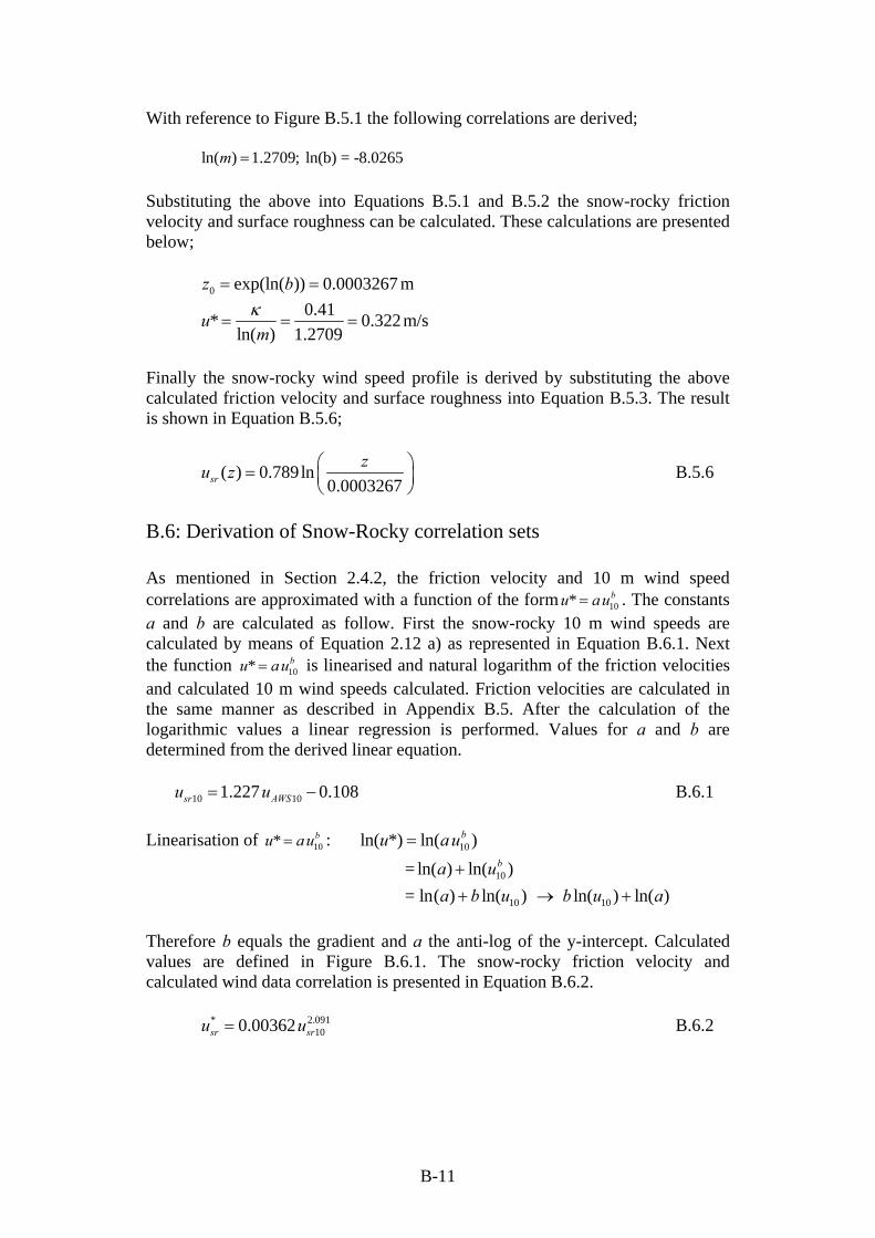
B-11
With reference to Figure B.5.1 the following correlations are derived; ln( ) 1.2709; ln(b) = -8.0265m Substituting the above into Equations B.5.1 and B.5.2 the snow-rocky friction velocity and surface roughness can be calculated. These calculations are presented below; 0 exp(ln( )) 0.0003267 mz b
0.41* 0.322m/s
ln( ) 1.2709u
m
Finally the snow-rocky wind speed profile is derived by substituting the above calculated friction velocity and surface roughness into Equation B.5.3. The result is shown in Equation B.5.6;
( ) 0.789ln0.0003267sr
zu z
B.5.6
B.6: Derivation of Snow-Rocky correlation sets As mentioned in Section 2.4.2, the friction velocity and 10 m wind speed correlations are approximated with a function of the form 10* bu au . The constants a and b are calculated as follow. First the snow-rocky 10 m wind speeds are calculated by means of Equation 2.12 a) as represented in Equation B.6.1. Next the function 10* bu au is linearised and natural logarithm of the friction velocities and calculated 10 m wind speeds calculated. Friction velocities are calculated in the same manner as described in Appendix B.5. After the calculation of the logarithmic values a linear regression is performed. Values for a and b are determined from the derived linear equation.
10 101.227 0.108sr AWSu u B.6.1
Linearisation of 10* bu au : 10ln( *) ln( ) bu au
10
10 10
= ln( ) ln( )
= ln( ) ln( ) ln( ) ln( )
ba u
a b u b u a
Therefore b equals the gradient and a the anti-log of the y-intercept. Calculated values are defined in Figure B.6.1. The snow-rocky friction velocity and calculated wind data correlation is presented in Equation B.6.2.
* 2.091100.00362sr sru u B.6.2

B-12
1.2 1.4 1.6 1.8 2 2.2 2.4 2.6 2.8-3.5
-3
-2.5
-2
-1.5
-1
-0.5
0
0.5
1
1.5
ln(usr10
) [m/s]
ln(u
* sr)
[m/s
]
Calculated
ln(u*sr
) = 2.091ln(usr10
)-5.621 (R2=0.81)
Figure B.6.1: Snow-rocky shear velocity and 10 m wind speed linear regression
results The derivation of snow-rocky friction velocity and surface roughness correlation is based on the method described in the above. Except a different approximation function and values are used. The approximation function linearised is of the form
0 ( ) /(2 )dz c u g . The natural logarithmic values of z0sr, c/2g and usr* are
calculated followed by performing a linear regression. The linear regression results and correlation are shown in Figure B.6.2.
0.2 0.25 0.3 0.35 0.40
0.01
0.02
0.03
0.04
0.05
0.06
0.07
0.08
0.09
0.1
u*sr
[m/s]
z0
sr [
m]
Calculated
z0sr
= 0.0863(u*sr
)3.272/(2g) (R2=0.63)
Figure B.6.2: Snow-rocky friction velocity and surface roughness correlation

B-13
B.7: The Vesleskarvet Wind Resource Map Generation Table B.7.1: Mesh and infrastructure dimensions Geometry Dimensions [m] Mesh 1240 x 1240 x 400 SANAE IV base represented by three rectangular blocks linked by two inter-sections
Block 1: 45 x 12 x 6 at 3 m AGL Block 2: 45 x 14 x 6 at 3 m AGL Block 3: 45 x 15 x 6 at 3 m AGL Intersection: 4 x 4 x 3 at 3 m AGL
Fuel bunkers are represented by six blocks of same dimension
4 x 4 x 3 at 4 m AGL
SHARE antennae are represented by T-shaped square tubes
Horizontal beam: 0.5 x 0.5 x 3 Vertical beam: 0.5 x 0.5 x 10
Table B.7.2: Boundary conditions and boundary locations Boundary (location)
Validation case Normal year case
Inlet (east vertical plane)
Velocity profile [m/s]: 0.237
( ) ln0.41 0.0000152
zu z
Turbulence profiles: 0.18839turk m2/s2
0.032769
( 0.00001518)z
m2/s3
Velocity profile [m/s]: 0.49979
( ) ln0.0001516
zu z
Turbulence profiles: 0.8323turk m2/s2
0.3043
( 0.0001516)z
m2/s3
Outlet (west vertical plane)
single flow split
Side symmetry (north and south vertical planes) Top symmetry (top plane)
standard, no-slip
Snow-rocky wall Snow-ice wall
rough wall
All other walls smooth wall
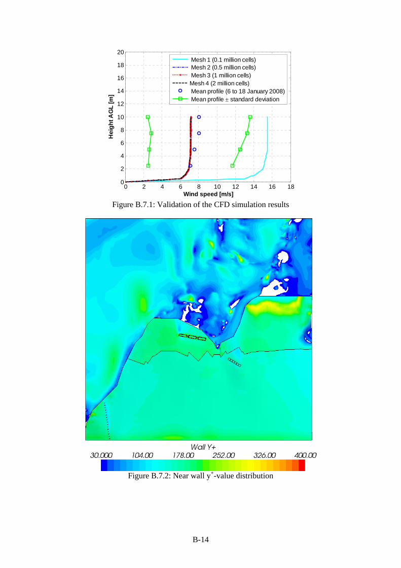
B-14
0 2 4 6 8 10 12 14 16 180
2
4
6
8
10
12
14
16
18
20
Wind speed [m/s]
Hei
gh
t A
GL
[m
]
Mesh 1 (0.1 million cells) Mesh 2 (0.5 million cells) Mesh 3 (1 million cells)Mesh 4 (2 million cells) Mean profile (6 to 18 January 2008) Mean profile standard deviation
Figure B.7.1: Validation of the CFD simulation results
Figure B.7.2: Near wall y+-value distribution
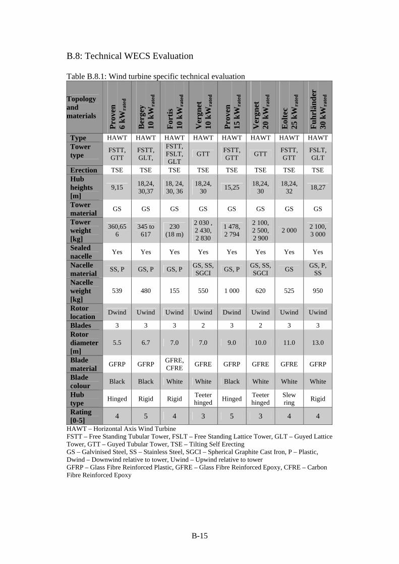
B-15
B.8: Technical WECS Evaluation Table B.8.1: Wind turbine specific technical evaluation
Topology and materials
Pro
ven
6
kW
rate
d
Ber
gey
10 k
Wra
ted
For
tis
10 k
Wra
ted
Ver
gnet
10
kW
rate
d
Pro
ven
15
kW
rate
d
Ver
gnet
20
kW
rate
d
Eol
tec
25 k
Wra
ted
Fu
hrl
änd
er
30 k
Wra
ted
Type HAWT HAWT HAWT HAWT HAWT HAWT HAWT HAWT Tower type
FSTT, GTT
FSTT, GLT,
FSTT, FSLT, GLT
GTT FSTT, GTT
GTT FSTT, GTT
FSLT, GLT
Erection TSE TSE TSE TSE TSE TSE TSE TSE Hub heights [m]
9,15 18,24, 30,37
18, 24, 30, 36
18,24, 30
15,25 18,24,
30 18,24,
32 18,27
Tower material
GS GS GS GS GS GS GS GS
Tower weight [kg]
360,656
345 to 617
230 (18 m)
2 030 , 2 430, 2 830
1 478, 2 794
2 100, 2 500, 2 900
2 000 2 100, 3 000
Sealed nacelle
Yes Yes Yes Yes Yes Yes Yes Yes
Nacelle material
SS, P GS, P GS, P GS, SS, SGCI
GS, P GS, SS, SGCI
GS GS, P,
SS
Nacelle weight [kg]
539 480 155 550 1 000 620 525 950
Rotor location
Dwind Uwind Uwind Uwind Dwind Uwind Uwind Uwind
Blades 3 3 3 2 3 2 3 3 Rotor diameter [m]
5.5 6.7 7.0 7.0 9.0 10.0 11.0 13.0
Blade material
GFRP GFRP GFRE, CFRE
GFRE GFRP GFRE GFRE GFRP
Blade colour
Black Black White White Black White White White
Hub type
Hinged Rigid Rigid Teeter hinged
Hinged Teeter hinged
Slew ring
Rigid
Rating [0-5]
4 5 4 3 5 3 4 4
HAWT – Horizontal Axis Wind Turbine FSTT – Free Standing Tubular Tower, FSLT – Free Standing Lattice Tower, GLT – Guyed Lattice Tower, GTT – Guyed Tubular Tower, TSE – Tilting Self Erecting GS – Galvinised Steel, SS – Stainless Steel, SGCI – Spherical Graphite Cast Iron, P – Plastic, Dwind – Downwind relative to tower, Uwind – Upwind relative to tower GFRP – Glass Fibre Reinforced Plastic, GFRE – Glass Fibre Reinforced Epoxy, CFRE – Carbon Fibre Reinforced Epoxy

B-16
Table B.8.2: Wind turbine specific power plant and control evaluation
PSP – Parallel Shafted Planetary, PG – Planetary Gearbox BPESG – Brushless Permanent Excited Synchronous Generator, GAG – Geared Asynchronous Generator TE– TEetering, PB – Parking Brake, BF – Blade Feathering Table B.8.3: Wind turbine specific operation related evaluation
Operation
Pro
ven
6
kW
rate
d
Ber
gey
10 k
Wra
ted
For
tis
10 k
Wra
ted
Ver
gnet
10
kW
rate
d
Pro
ven
15
kW
rate
d
Ver
gnet
20
kW
rate
d
Eol
tec
25 k
Wra
ted
Fu
hrl
änd
er
30 k
Wra
ted
Cut-in wind speed [m/s] 2.5 3.1 3.0 4.5 2.5 4.5 2.6 2.5
Cut-out wind speed [m/s] 70 54 60 70 65 60 60 25
Rated wind speed [m/s] 12 13.8 13 12 12 16 11 12
Survival wind speed [m/s] 70 54 60 70 65 60 60 67
Rated rotor rotational speed [rpm]
200 310 280 135 or
150 150 139 145
47 or 70
Typical annual yield [MWhe/a] 12 30 24 - 30 - 156 129
Operating temperature range [°C]
-40 to
+45
-40 to
+60
-30 to
+50
-30 to
+40
-40 to
+45
-30 to
+40
-40 to
+50
-20 to
+50 Rating [0-5] 5 4 4 3 4 3 3 2
Drive train and control
Pro
ven
6
kW
rate
d
Ber
gey
10 k
Wra
ted
For
tis
10 k
Wra
ted
Ver
gnet
10
kW
rate
d
Pro
ven
15
kW
rate
d
Ver
gnet
20
kW
rate
d
Eol
tec
25 k
Wra
ted
Fu
hrl
änd
er
30 k
Wra
ted
Gearbox design
None None None
PSP
None
PSP
None 2 stage
PG
Generator design
BPESG
BPESG
BPESG
GAG BPES
G GAG
BPESG
GAG
Rotor speed control
Furling stall
Furling stall
Stall T Furling
stall T Stall Stall
Rotor brake None Tail vane
furling
Tail vane
furling PB None PB BF
Blade tip and
disk brakes
Yaw control Free Tail vane
Tail vane
Tail vane
Free Tail vane
Tail vane
Yaw motor
Rating [0-5] 5 4 4 2 5 2 4 2

B-17
Table B.8.4: Wind turbine specific performance evaluation
Theoretical performance based on the Vesleskarvet climate P
rove
n
6 k
Wra
ted
Ber
gey
10 k
Wra
ted
For
tis
10 k
Wra
ted
Ver
gnet
10
kW
rate
d
Pro
ven
15
kW
rate
d
Ver
gnet
20
kW
rate
d
Eol
tec
25 k
Wra
ted
Fu
hrl
änd
er
30 k
Wra
ted
Specific annual yield at LHH [kWhe/m
2 a]
1 995 1 427 1 040 1 726 1 356 1 383 1 668 836
Annual yield at LHH and temperature[MWhe/a]
38.7 50.3 40.0 66.4 86.3 108.6 158.5 110.9
Operation availability [%]
92.5 89.4 87.7 84.7 92.5 84.7 92.6 63.3
Hours operational at rated wind speed [h/a]
769 727 737 747 749 510 685 747
Max. power coefficient at LHH [wind speed in m/s]
0.55 [5]
0.35 [5]
0.35 [6]
0.33 [8]
0.23 [4]
0.26 [8]
0.40 [9]
0.41 [3]
Annual capacity factor at LHH [%]
73.6 57.4 46.6 77.3 65.6 63.2 72.4 42.2
Rating [0-5] 5 4 5 4 4 3 4 2 LHH – Lowest Hub Height specified by wind turbine manufacturer

C-1
Appendix C: SANAE IV Energy Systems
C.1: The SANAE IV Water, Waste Water Treatment, Humidification and Ventilation and Overhead Control Systems
C.1.1 Water System
All water consumed at SANAE IV is produced by the smelting of snow and ice with a multiple three phase electric heater system. The snow smelter, the most electric energy intensive load, consists of two storage tanks, two circulation pumps and six 15 kWrated heating elements. The system layout is represented in Figure CD.2.2 in Appendix CD.2.1. The snow smelter has an estimated summer minimum daily electrical energy demand of 819 kWhe which is equivalent to a 34 kWe load. Water is pumped from the snow smelter tanks to the base situated, twelve-day storage tanks. These tanks are capable of storing up to 46 000 L of water. The tanks supply water to four water circuits namely the closed primary hot water circuit, the Fan Coil Unit (FCU) water circuit, the domestic hot circuit and domestic cold water circuit. These water circuit layouts are illustrated in Figures CD.2.3 and CD.2.4 in Appendix CD.2.1. Waste heat recovered from the power system diesel engine cooling water circuits and exhaust gasses is supplied to the primary hot water circuit. This primary hot water circuit acts as a thermal energy storage system. This system distributes heat via heat exchangers to the FCU and domestic hot water circuits. The FCU water circuit supplies heat for space heating to the air ventilation units located in the SANAE IB base sections. Hot water for domestic use is supplied and circulated with the domestic hot water circuit. Six in-line heaters of 60 kWrated in total capacity ensure that the water is kept between 55 °C and 60 °C. The cold water circuit circulates cold water between the day storage tanks and SANAE IV base sections. Three 30 kWrated in-line heaters are utilised to prevent freezing. Almost all of the thermal energy consumed by the base is extracted from the diesel engine waste heat recovery units whereas in-line heaters only replace lost heat from the domestic hot warm system.
C.1.3 Waste Water Treatment System
SANAE IV processes its own waste and disposes its treated waste water. Initially, waste water is temporarily stored in two tanks located in the AB and BC base interconnections. This water is then mechanically filtered, to ensure that no large residue enters the bio-filtration system. Hereafter the water is chemically and biological treated and disposed. Solid waste are containerised and shipped back to South Africa for further processing. This small water treatment plant mostly consists of pumps. The system has an overall capacity of 6.75 kWrated.

C-2
C.1.3 Ventilation and Humidification System
The SANAE IV base interior is heated with three air ventilation systems situated within each base section. The ventilation system is controlled by a PLC system. As previously mentioned, the FCU water circuit supplies the needed thermal energy to heat the cold air drawn from outside. Variable speed fans are used to control the amount of heat transferred to the separate base sections. In addition each room within each base section is equipped with 2 kWrated skirting heaters. The heated dry Antarctic air is humidified with two humidifiers located in the AB and BC base interlinking sections. These fully automatic humidifiers release steam if the relative humidity drops to below 60 %. The overall rated power capacity of the air heating, ventilation and humidification system amounts to about 34 kWrated. The system layout is presented in Figure CD.2.5 in Appendix CD.2.1.
C.1.4 Overhead Control System
According to Cencelli (2002), the overhead control system consists of a clustered programmable logic controller (PLC) systems and a cluster of power electronic controllers. The PLC cluster which controls the base heating and ventilation systems consists of the main plant PLC 1 to 3 and the FCU PLC network. Power production, conditioning and regulation are controlled by three GENCON II systems. The function of each of these control clusters is described below. Main plant PLC 1 controls the base temperature by regulating the FCU water temperature which supplies heat to the ventilation systems. Main plant PLC 2 is responsible for the regulation of the diesel-electric generator coolant temperature, hence, preventing generator overheating by either controlling the primary hot water flow rate or dumping heat via a heat dump fan unit. Main PLC 3 ensures that the domestic hot and cold water circuits are at their respective temperatures. This PLC will energise the inline heaters as to prevent the circuit freezing. Lastly, the FCU PLC network consists of three separate FCU PLCs which controls the fans utilised by the air ventilation. Each of the three diesel-electric generators is separately controlled by a GENCON II PLC/power electronic system. STANDBY V1.7 software ensures power system communication, power synchronised and load matching. These control units ensure voltage and frequency stability by regulating the generator voltage and diesel engine rotational speed (with a fuel solenoid). The true root mean square phase voltages, currents, active and reactive power and network frequency are monitored but not logged by the overhead computer. This processor also links these controllers.

C-3
Figure C.1.1: Section specific peak power demand breakdown
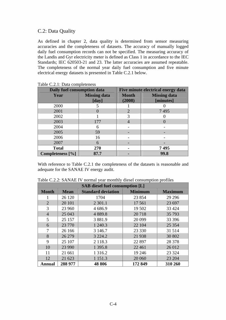
C-4
C.2: Data Quality
As defined in chapter 2, data quality is determined from sensor measuring accuracies and the completeness of datasets. The accuracy of manually logged daily fuel consumption records can not be specified. The measuring accuracy of the Landis and Gyr electricity meter is defined as Class 1 in accordance to the IEC Standards; IEC 620503-21 and 23. The latter accuracies are assumed repeatable. The completeness of the normal year daily fuel consumption and five minute electrical energy datasets is presented in Table C.2.1 below. Table C.2.1: Data completeness
Daily fuel consumption data Five minute electrical energy data Year Missing data
[day] Month (2008)
Missing data [minutes]
2000 5 1 0 2001 0 2 7 495 2002 1 3 0 2003 177 4 0 2004 6 - - 2005 59 - - 2006 16 - - 2007 6 - - Total 270 - 7 495
Completeness [%] 87.7 - 99.8 With reference to Table C.2.1 the completeness of the datasets is reasonable and adequate for the SANAE IV energy audit. Table C.2.2: SANAE IV normal year monthly diesel consumption profiles
SAB diesel fuel consumption [L] Month Mean Standard deviation Minimum Maximum
1 26 120 1704 23 854 29 296 2 20 101 2 301.1 17 561 23 697 3 23 960 4 686.9 19 502 33 424 4 25 043 4 889.8 20 718 35 793 5 25 157 3 881.9 20 099 33 396 6 23 770 1 240.3 22 104 25 354 7 26 166 3 146.7 23 330 31 514 8 26 279 3 224.2 21 938 30 802 9 25 107 2 118.3 22 897 28 378 10 23 990 1 395.8 22 461 26 012 11 21 661 1 316.2 19 246 23 324 12 21 623 1 151.3 20 060 23 204
Annual 288 977 48 806 172 849 310 260

C-5
Table C.2.3: SANAE IV normal year daily diesel consumption profiles
Month Day
Jan Feb Mar Apr May Jun Jul Aug Sep Oct Nov Dec 1 817 894 797 829 778 887 798 816 839 776 801 782 2 752 757 849 831 900 715 805 750 837 840 779 680 3 902 874 712 817 908 947 826 923 750 908 799 675 4 874 579 785 988 785 819 891 891 839 831 670 611 5 771 827 728 861 868 829 745 950 810 821 656 640 6 796 765 871 1 022 761 709 920 955 841 836 871 567 7 950 747 760 968 808 755 810 919 917 864 719 692 8 841 869 801 865 869 913 819 880 903 771 701 607 9 946 689 749 841 838 767 756 927 914 757 816 683 10 817 878 741 849 786 815 897 844 787 764 690 629 11 908 707 771 825 850 841 758 853 860 743 768 689 12 897 693 800 863 777 743 864 841 791 745 537 648 13 883 894 887 863 851 755 850 853 885 1 012 612 704 14 948 667 603 925 803 702 824 788 844 771 770 639 15 717 835 825 897 711 751 906 783 723 841 1 001 741 16 1 006 723 787 871 764 807 944 778 862 688 629 675 17 806 806 857 827 937 707 956 893 700 807 759 513 18 927 619 767 825 886 851 859 852 844 831 697 699 19 911 716 750 901 793 715 815 890 937 653 778 746 20 1 006 715 793 735 781 784 824 838 799 735 725 688 21 1 016 845 757 906 837 918 891 813 806 838 712 756 22 981 637 805 1055 791 818 860 795 866 577 720 692 23 1 083 754 898 827 933 1 023 857 840 821 778 753 687 24 878 821 757 878 829 803 875 788 910 623 583 794 25 1 081 897 775 1017 907 768 908 830 793 777 626 728 26 747 720 815 789 815 811 765 815 745 670 631 772 27 883 838 737 871 1 000 827 884 918 856 743 785 814 28 729 1 145 837 815 763 889 846 871 854 713 823 852 29 829 - 753 821 681 779 842 772 738 776 738 820 30 927 - 835 737 869 788 827 850 749 757 694 1 05931 831 - 823 - 814 - 817 843 - 799 - 887

C-6
0 50 100 150 200 250 300 3501500
2000
2500
3000
3500
4000
4500
Day
En
erg
y [
kW
he]
Estimation based on 2000 to 2007 fuel records
Figure C.2.1: Normal year SANAE IV daily electrical energy demand
The data presented in Table C.2.1 is represented in Appendix CD.2.1
Table C.2.4: SANAE IV normal year power frequency distribution
Power bin median [kWe]
Frequency [h/a]
Power bin median [kWe]
Frequency [h/a]
5 4 145 599 15 19 155 307 25 15 165 216 35 15 175 159 45 42 185 91 55 34 195 95 65 61 205 49 75 205 215 38 85 375 225 30 95 1 305 235 30 105 1 415 245 23 115 1 529 255 11 125 1 365 265 15 135 683 275 30

C-7
40 60 80 100 120 140 160 180 2000
0.5
1
1.5
2
2.5
3
Power [kWe]
Fre
qu
en
cy
[h
/da
y]
Bin size: 5 kWe
Measured (January to February 2008)
Figure C.2.2: Summer diurnal load frequency distribution
40 60 80 100 120 140 160 180 2000
0.5
1
1.5
2
2.5
3
3.5
4
Power [kWe]
Fre
qu
en
cy
[h
/da
y]
Bin size: 5 kWe
Measured (March to April 2008)
Figure C.2.3: Winter diurnal load frequency distribution
The data presented in Figures C.2.2 and C.2.3 is represented in Tables CD.2.2 and CD.2.3, respectively, in Appendix CD.2.1.

C-8
C.3: Load Matching and Wind Power Penetration Issues
Jan Feb Mrt Apr May Jun Jul Aug Sep Oct Nov Dec0
0.5
1
1.5
2
2.5
3
Month
Monthly load profile (Pavg
= 3 557.8 kWe)
Normal year wind power density at 10 m AGL ((P/A)
avg = 0.797 kW/m2)
Figure C.3.1: Normalised monthly load and wind power profile comparisons
The data presented in Figure C.3.1 is represented in the table below.
Month Normalised load profile Normalised wind speed profile 1 1.08 0.34 2 0.92 0.55 3 0.98 2.12 4 1.07 1.05 5 1.02 0.94 6 1.00 1.37 7 1.05 1.07 8 1.06 1.42 9 1.04 0.97 10 0.97 0.91 11 0.92 0.91 12 0.89 0.35

C-9
Table C.3.1: Second or slave diesel-electric generator operation frequency Current SANAE IV power system control limits Lower limit: 140 kWe Upper limit: 162 kWe
Changed SANAE IV power system control limits Lower limit: 140 kWe Upper limit: 170 kWe
Instantaneous penetration ratio [%]
Typical summer
Typical winter
Typical summer
Typical winter
0 25 15 25 24 5 23 15 17 26 10 29 8 17 14 15 9 7 9 2 20 1 10 11 0 25 0 3 7 0 30 0 0 1 0 35 0 0 0 0 40 0 0 0 0 45 0 0 0 0 50 0 0 0 0
Table C.3.2: Wind turbine specific average penetration ratios
Wind power penetration ratios
Pro
ven
6
kW
rate
d
Ber
gey
10 k
Wra
ted
For
tis
10 k
Wra
ted
Ver
gnet
10
kW
rate
d
Pro
ven
15
kW
rate
d
Ver
gnet
20
kW
rate
d
Eol
tec
25 k
Wra
ted
Fu
hrl
änd
er
30 k
Wra
ted
Average [%] 4 5 4 6 8 11 16 11 Wind turbine rating [0-5] 3 3 3 3 2 2 4 2
0 2 4 6 8 10 12 14 16 18 20 22 240.97
0.975
0.98
0.985
0.99
0.995
1
Hour
Po
we
r fa
cto
r
Summer (January 2008 to February 2008) Winter (March 2008 to April 2008)
Figure C.3.2: Calculated seasonal power factors

C-10
Table C.3.3: Wind turbine electrical compatibility
Electrical design
Pro
ven
6
kW
rate
d
Ber
gey
10 k
Wra
ted
For
tis
10 k
Wra
ted
Ver
gnet
10
kW
rate
d
Pro
ven
15
kW
rate
d
Ver
gnet
20
kW
rate
d
Eol
tec
25 k
Wra
ted
Fu
hrl
änd
er
30 k
Wra
ted
Generator type
BPESG BPESG BPESG GAG BPESG GAG BPESG GAG
Grid connection devices required
I I I C I C I C
Inverter-grid terminal voltage [VAC]
230 or
400
240 or
400 400 400 230
400 or
690 400 400
Inverter voltage phases
1 or 3 1 or 3 3 3 1 3 3 3
Output frequency [Hz]
50 50 50 50 50 50 50 50
Wind turbine rating [0 - 5]
4 5 5 3 3 3 4 3
BPESG – Brushless Permanently Excited Synchronous Generator GAG – Geared Asynchronous Generator I – Inverter C – Converter

D-1
Appendix D: Wind Turbine Micro-Siting D.1: Vesleskarvet Wind Turbulence Map
Fig
ure
D.1
.1: S
pati
al V
esle
skar
vet w
ind
turb
ulen
ce in
tens
ity d
istr
ibut
ion
at 1
0 m
AG
L

D-2
D.2: SANAE IV and its surroundings
Fig
ure
D.2
.1: A
eria
l pho
togr
aph
of S
AN
AE
IV
loca
ted
on V
esle
skar
vet a
s vi
ewed
fro
m th
e so
uth
(Hof
mey
r, 2
008)

D-3
Fig
ure
D.2
.2: V
iew
shed
s as
vie
wed
fro
m th
e S
AN
AE
IV
bas
e (S
tand
er,2
008)
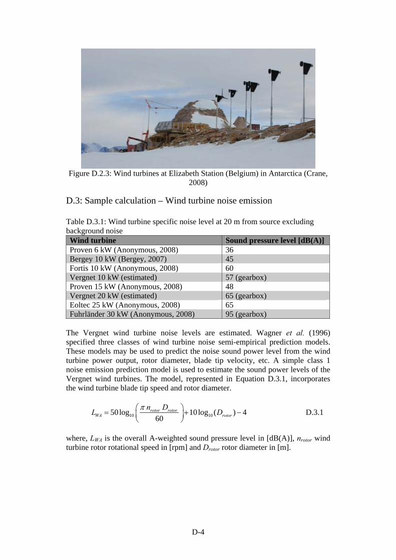
D-4
Figure D.2.3: Wind turbines at Elizabeth Station (Belgium) in Antarctica (Crane,
2008)
D.3: Sample calculation – Wind turbine noise emission Table D.3.1: Wind turbine specific noise level at 20 m from source excluding background noise Wind turbine Sound pressure level [dB(A)] Proven 6 kW (Anonymous, 2008) 36 Bergey 10 kW (Bergey, 2007) 45 Fortis 10 kW (Anonymous, 2008) 60 Vergnet 10 kW (estimated) 57 (gearbox) Proven 15 kW (Anonymous, 2008) 48 Vergnet 20 kW (estimated) 65 (gearbox) Eoltec 25 kW (Anonymous, 2008) 65 Fuhrländer 30 kW (Anonymous, 2008) 95 (gearbox)
The Vergnet wind turbine noise levels are estimated. Wagner et al. (1996) specified three classes of wind turbine noise semi-empirical prediction models. These models may be used to predict the noise sound power level from the wind turbine power output, rotor diameter, blade tip velocity, etc. A simple class 1 noise emission prediction model is used to estimate the sound power levels of the Vergnet wind turbines. The model, represented in Equation D.3.1, incorporates the wind turbine blade tip speed and rotor diameter.
10 1050 log 10log ( ) 460
rotor rotorWA rotor
n DL D
D.3.1
where, LWA is the overall A-weighted sound pressure level in [dB(A)], nrotor wind turbine rotor rotational speed in [rpm] and Drotor rotor diameter in [m].

D-5
Rotor diameters and rated rotor rotational speeds of the two Vergnet wind turbines are:
Vergnet 10 kW: Drotor = 7 m, nrotor = 150 rpm Vergnet 20 kW: Drotor = 10 m, nrotor = 139 rpm
The calculated sound pressure levels expected at wind turbine nacelles are:
Vergnet 10 kW: 91 dB(A) Vergnet 20 kW: 99 dB(A)
These wind turbines both utilise a gearbox to reduce rotor rotational speed to the required generator shaft rotational speed. Thus higher than the above calculated sound pressure levels may be expected. With a hemispherical noise propagation model as presented in Equation D.3.2 the wind turbine specific sound power levels at a distance 20 m were estimated. These estimations exclude the noise damping effect of background noise.
21010log 2p WA absorpL L R R D.3.2
where, Lp is the sound pressure level in [dB(A)] expected at a distance R in [m] from the noise source which emits at a power level LWA in [dB(A)]. A sound absorption coefficient of αabsorp = 0.005 dB(A)/m was assumed.
D.4: Technical Site Survey
Figure D.4.1: The two cargo transport routes here indicated in red (Stander, 2008)
SA Bukta
Akta Bukta

D-6
Figure D.4.2: Vesleskarvet access routes and foundations specific areas
(Photograph by Hofmeyr, 2008)
D.4.1 Proposed wind turbine foundations
The wind turbine foundations are to be designed to support the wind turbine weight, to resist tower base shear forces, wind turbine excited vibrations and bending moments induced by wind loading. Specific to SANAE IV the additional impact of the expected low temperatures and associated high wind conditions must be analysed. Furthermore wind turbine foundation size also depends on the ground structure and the allowed construction material. The orography specific foundation designs suggested for the proposed wind turbine are described below. In the snow-rocky area a rock anchored pylon foundation design similar to the SANAE IV base foundation is preferred. Part of the foundation is shown in Figure D.4.3. Typically vertical oversized shafts are drilled into the bedrock after which the pylons are sunked and freezed to the rock. The foundation stability depends on the shaft depth, pylon diameter and wall thickness, ice density distribution along the pylon length, etc. Depending on the wind turbine size an arranged multiple pylon foundation as shown in Figure D.4.4 may be constructed. This structure common to permafrost wind turbine foundations consists of base plate, possible anchor rods and wind turbine tower connection flange. Detail information on freeze-back pylon and permafrost multi-pylon foundation shown in Figure D.4.4 were described by Petrie et al. (2007) and included in Appendix CD.3.

D-7
Figure D.4.3: SANAE IV base freeze-back pylon foundation (Stander, 2008)
Figure D.4.4: Photographs of a a) freeze-back pylon and b) a permafrost multi-
pylon foundation (Laakso et al., 2005) A snow-ice site will require an entirely different wind turbine foundation design. Typically a snow-ice foundation consists of a large horizontal base structure which is submerged at a required depth below the snow-ice surface. The base frame connects the snow-ice buried base with the wind turbine tower. In this design the snow-ice mixture replaces concrete in typical gravity type foundation. Thus overall foundation stability depends on the foundation depth and the density of the compacted snow-ice mixture. Thus unlike rock anchored foundation these foundations limit the standalone wind turbine tower height. Therefore these wind turbine foundations are usually assisted by guide cabling which improve stability through load sharing. An example of such a foundation is described by to El Naggar et al. (2000). The 20 kW vertical axis wind turbine utilised by the German Antarctic base is supported by a snow buried foundation. With a 10 m hub height the wind turbine foundation consists of three risible base frames. The foundation base is buried at depth of approximately 2 m. The foundation design and wind turbine are shown in Figure D.4.5.

D-8
Figure D.4.5: Schematic of the Neumayer wind turbine snow-ice foundation (El
Naggar et al., 2000) and a photograph of the wind turbine (Stander, 2008)
D.5: Sample calculation – Blade and ice throw estimations
D.5.1 Blade throw
The distance which a blade or blade fragment may travel depends on a number of variables such as the size and the weight of blade or fragment, hub height, rotor rotational speed, nature of blade fracture, manner in which the blade is liberated, wind conditions, etc. As a first estimate the blade throw estimation was simplified by assuming that the blade fractured at its root and travels with a speed equal to its centroid speed. Air friction and wind conditions were neglected. The calculation of the maximum safe distances relative to the wind turbine was based on the schematic shown here in Figure D.5.1. Wind turbine data are tabled in Table D.5.1.
Figure D.5.1: Schematic of a simplified wind turbine blade trajectory

D-9
Table D.5.1: Wind turbine specific information
Data
Pro
ven
6
kW
Ber
gey
10 k
W
For
tis
10 k
W
Ver
gnet
10
kW
Pro
ven
15
kW
Ver
gnet
20
kW
Eol
tec
25 k
W
Fu
hrl
änd
er
30 k
W
Blade length [m] 2.7 3.4 3.3 3.3 4.5 5.0 5.5 6.5 Rotational speed [rpm]
200 310 300 150 150 139 140 70
Hub heights [m] 9 18 18 18 15 18 18 18 The basic kinematic equations applied are represented in Equations D.5.1 to D.5.3. A constant gravitational acceleration of g = 9.81 m/s2 was assumed.
60
blade rotorc
l nv
D.5.1
cos(45 ) cx cy cv v v D.5.2
21
2 2i f
i
v vs v t g t t
D.5.3
where vc,vcx and vcy are the blade centroid speeds in vector components in [m/s], lblade the blade length in [m], Nrotor the wind turbine rated rotor rational speed in [r.p.m], vi,f the cartesian velocity components in [m/s], t the time in [s] and s the distance in [m]. The safe distance estimations are specified in Table D.5.2.
D.5.2 Ice shedding
Seifert et al. (2003) defined two empirical ice shedding prediction models. One model predicts the ice shedding distance for an operational wind turbine and the second predicts the ice fall distance for a parked wind turbine. These models are represented in Equations D.5.4 and D.5.5, respectively. ( )1.5op rotor hd D z D.5.4
0.5
15rotor h
park
D zd u
D.5.5
where dop and dpark are the respective ice shedding distances in [m] for when the wind turbine is operational and park, Drotor the rotor diameter in [m], h the hub height in [m] and u the average hub height wind speed in [m/s]. The safe distance estimations are specified in Table D.5.2.

D-10
Table D.5.2: Wind turbine specific blade and ice throw safe distances
Estimated safe distances
Pro
ven
6
kW
Ber
gey
10 k
W
For
tis
10 k
W
Ver
gnet
10
kW
Pro
ven
15
kW
Ver
gnet
20
kW
Eol
tec
25 k
W
Fu
hrl
änd
er
30 k
W
Average wind speed at hub height [m/s]
12.2 13.1 13.1 13.1 12.9 13.1 13.1 13.1
Maximum blade throw distance [m]
91 312 293 85 143 154 185 75
Ice fall distance when wind turbine is parked [m]
10 19 19 19 17 20 21 21
Ice shedding safe distance when wind turbine in operation [m]
22 38 38 38 36 42 44 47

E-1
Appendix E: Wind-Diesel System Economy
E.1: Financial Data Table E.1 specifies the SANAE IV annual diesel-electric generator system O&M cost estimate, general interest, inflation and currency exchanges rates of May 2008. The general interest, inflation and currency exchanges rates are based on values specified by SARB (2008) and Shell (2008). Table E.1.1: Financial related data
The SANAE IV diesel-electrical power system financial related data
Normal year SAB diesel fuel consumption [L/a] 288 976
2008 SAB diesel purchase price [ZAR/L] -6.34
2008 SAB diesel price at SANAE IV [ZAR/L] -19.02
Estimated annual O&M cost [ZAR] -147 377
Normal year energy production [kWhe/a] 1 024 971
Normal year operating hours [hours/a] 9 550
Diesel-electric generator electrical efficiency [%] 36.5
SAB diesel energy density per volume [kWh/L] 9.81
Estimated O&M cost saving due to wind power [ZAR/a] See Table E.2.1
Economic data (May 2008)
Cumulative external cost based diesel consumed [ZAR/L] 6.59
Interest rate on lent capital [%] 15.0
General inflation rate [%] 10.1
Estimated combined O&M cost escalation rate [%] 2
Estimated fuel escalation rate [%] 2
Estimated escalation rate of external costs [%] 1
Dollar exchange rate [ZAR/US$] 7.59
Euro exchange rate [ZAR/Euro] 11.73
Pound exchange rate [ZAR/Pound] 14.86
Crude oil price [US$/barrel] 105.16

E-2
In Table E.2.1 wind turbine operational availabilities included the compulsory 24 h annual service. The wind turbine purchase prices are based on the May 2008 currency exchange rates. These prices include the added costs of cold climate modifications to wind turbine tower, rotor and control system. The SANAE IV wind turbine transportation, site preparation, installation and commissioning cost estimations are based on an Australian Antarctic base wind-diesel project cost breakdown as presented by Frye (2006). Wind turbine transportation cost for the packaging and transportation of wind turbine from South Africa to SANAE IV is estimated at 3 % of the wind turbine purchase price. The site preparation cost which includes the foundation, grid switch gear and cabling costs is estimated at 7 % of the wind turbine purchase price. Wind turbine installation and commissioning cost which include installation equipment, project management and testing costs is estimated at 10 % of the wind turbine purchase price. A wind turbine decommissioning cost is estimated at 5 % of the wind turbine purchase price. The total capital investment associated with the proposed SANAE wind-diesel system is the sum of wind turbine purchase price, site preparation, transportation, installation and commissioning and decommissioning costs. As a matter of clarity, the SANAE IV wind-diesel system options listed in Table E.2.1 are named after the integrated wind turbine. For example the wind-diesel system which incorporates the Proven 6 kW wind turbine is named the Proven6 wind-diesel system.
E.2: Proven6 Wind-Diesel System Economic Assessment
E.2.1 Calculation of the Net Present Values of Costs and Savings
The inflated NPV of costs associated with the Proven6 wind-diesel system are calculated by means of Equations 5.1 and 5.2 and financial data provided in Tables E.1.1 and E.2.1. The inflated NPV of costs after the first year equals the total cumulative costs at the end of that year brought back by an interest rate of 15 %. These costs are tabulated in Table E.3.
1
costs1
(1 )( )
(1 )
jN
jj
iNPV TC F OM
r
E.1
0
1
(1 0.101)[ ] 5548970[ ] 5147759.13 ZAR
(1 0.15)NPV ZAR ZAR
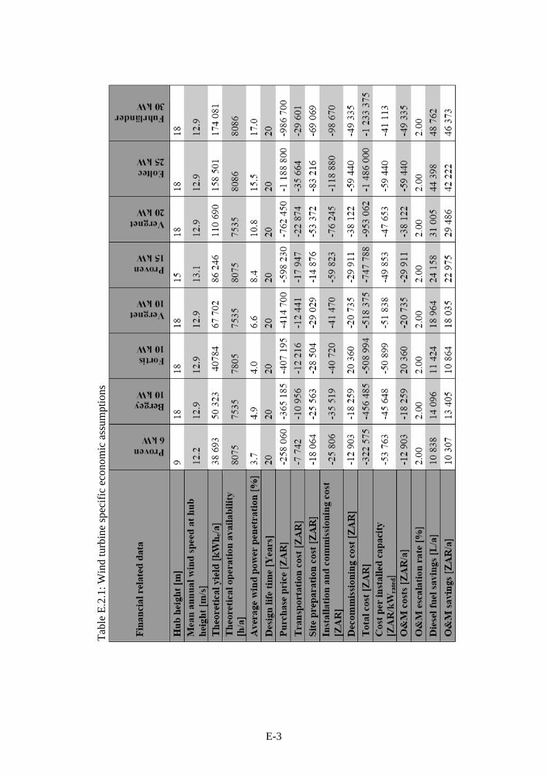
E-3
Tab
le E
.2.1
: Win
d tu
rbin
e sp
ecif
ic e
cono
mic
ass
umpt
ions

E-4
The NPV of savings generated by the Proven6 wind-diesel system were calculated subtracting the diesel system NPVcosts form the wind diesel system NPVcosts, as shown in Equation E.2.
savings WD DNPV NPV NPV E.2
[ ] 14461174.20[ ] 1466752.71[ ] 206418.52 ZARsavingsNPV ZAR ZAR ZAR
E.2.2 Calculation of the IRR
The Proven6 wind-diesel system IRR is calculated with the help the Matlab v.7 based function. Based on Equation 5.3 and the calculated savings tabulated in Table E.2.2 the IRR of the Proven6 wind-diesel is calculated as follow;
1
1
(1 )( ) 0
(1 )
jN
jj
iLCS LCC
IRR
E.3
0 18 19
1 19 20
1 0.101 (1 0.101) (1 0.101)322575 207613 .... 296523 302453 0
(1 0.536) (1 0.536) (1 0.536)
The investment associated with the Proven 6 kW wind turbine has an IRR of approximately 54 %.
E.2.3 Calculation of the energy conversion cost
The cost of electrical energy produced by the Proven6 wind-diesel power system is calculated with Equation 5.4 and the value listed at the bottom of Table E.2.2.
N
N
LCCCOE
E
E.4
ee
134825176.00[ZAR][ZAR/kWh ] 6.58 ZAR/kWh
e 20(1024971[kWh ])COE
Therefore the cost of energy generated by the Proven6 wind-diesel system is approximately 6.58 ZAR/kWhe.

E-5
Tab
le E
.2.2
: Cal
cula
ted
Pro
ven6
Win
d-D
iese
l (W
D)
pow
er s
yste
m a
nd S
AN
AE
IV
Die
sel-
elec
tric
(D
) sy
stem
life
cyc
le c
osts

E-6
Tab
le E
.2.3
: Cal
cula
ted
NP
V o
f co
sts
in [
ZA
R]
rela
ted
to p
ropo
sed
win
d-di
esel
pow
er s
yste
ms
and
SA
NA
E I
V d
iese
l-el
ectr
ic s
yste
m

E-7
E.3: Economic Evaluation of the SANAE IV Wind-Diesel System Table E.3.1: Proposed wind-diesel power system economic evaluation
-100 -80 -60 -40 -20 0 20 40 60 80 100-100
-50
0
50
100
150
200
250
Deviation [%]
NP
V o
f s
av
ing
s d
ev
iati
on
s [
%]
Diesel fuel escalation rate Interest rate General inflation rate Wind turbine purchase price
Figure E.3.1: Results of the Vergnet10 wind-diesel system economic sensitivity
analysis
Economic performance parameters
Pro
ven
6
Ber
gey1
0
For
tis1
0
Ver
gnet
10
Pro
ven
15
Ver
gnet
20
Eol
tec2
5
Fu
hrl
änd
e r3
0
NPV of savings exc. externalities [106 ZAR]
2.58 3.30 2.46 4.59 5.71 7.35 10.3 12.0
NPV of savings inc. externalities [106 ZAR]
2.63 3.36 2.50 4.67 5.81 7.66 10.5 12.2
IRR [%] 54 49 33 59 51 52 47 64 Payback period [Years]
2 3 4 2 3 3 3 2
COE [ZAR/kWhe] 6.58 6.58 6.57 6.39 6.28 6.12 5.82 5.71 Energy production cost reduction [%]
3.74 3.74 3.82 6.77 8.72 11.5 17.2 19.5
Wind turbine rating [0-5]
5 4 3 5 4 4 3 5

F-1
Appendix F: Market Assessment
F.1: Market Assessment Results
Fu
hrl
änd
er
> 1
000
Yes
Yes
1988
7 Inst
alla
tion
http
://w
ww
.fu
hrla
ende
r.de
poss
ible
IEC
61
400-
2 de
sign
st
anda
rd
Eol
tec
> 1
00
No
Yes
2001
2 Non
e
http
://w
ww
.eol
tec.
com
po
ssib
le
IEC
61
400-
2 de
sign
st
anda
rd
Ver
gnet
> 6
00
Yes
Yes
1988
5 Non
e
http
://w
ww
.ver
gnet
.fr
- -
For
its
> 6
000
Yes
Yes
1981
4 Inst
alla
tion
http
://w
ww
.for
tisw
inde
nerg
y.co
m
5 ye
ar
DE
A
cert
ifie
d
Ber
gey
> 2
000
Yes
Yes
1977
3 Inst
alla
tion
http
://w
ww
.ber
gey.
com
/Exa
mpl
es.h
tm
5 ye
ar
Tes
ted
by
NR
EL
Pro
ven
> 1
500
Yes
Yes
1982
3 Inst
alla
tion
http
://w
ww
.pr
oven
ener
gy.
co.u
k 5
year
BW
EA
ce
rtif
ied
and
IE
C 6
1400
-2
desi
gn
stan
dard
Mar
ket
cri
teri
a
Nu
mb
er in
stal
led
Col
d c
lim
ate
oper
atio
n
exp
erie
nce
Win
d-d
iese
l exp
erie
nce
Est
abli
shm
ent
Nu
mb
er o
f w
ind
tu
rbin
es
on m
ark
et
A S
outh
Afr
ican
re
sell
er/i
nst
alla
tion
Cu
stom
ers
or p
roje
cts
Ser
vice
pla
n
Cer
tifi
cati
on o
r st
and
ard
Tab
le F
.1.1
: Win
d tu
rbin
e m
anuf
actu
rer
asse
ssm
ent r
esul
ts

F-2
Table F.1.2: Wind turbine specific details
Details
Pro
ven
6
kW
Ber
gey
10 k
W
For
tis
10 k
W
Ver
gnet
10
kW
Pro
ven
15
kW
Ver
gnet
20
kW
Eol
tec
25 k
W
Fu
hrl
änd
er
30 k
W
Country SCOT USA NL FRA SCOT FRA FRA GER Topology
HAWT HAWT HAWT HAWT HAWT HAWT HAWT HAWT
LHH [m] 9 18 18 18 15 18 18 18 Rotor position
Dwind Uwind Uwind Uwind Dwind Uwind Uwind Uwind
Rotor diameter [m]
5.5 6.7 7.0 7.0 9.0 10.0 11.0 13.0
Number of blades
3 3 3 2 3 2 3 3
Cut-in wind speed [m/s]
2.5 3.1 3.0 4.5 2.5 4.5 2.6 2.5
Rated wind speed [m/s]
12 13.8 13 12 12 16 11 12
Cut-out wind speed [m/s]
70 54 60 70 65 60 60 25
Typical annual yield [MWhe/a]
12.0 28.8 22.0 - 30.0 - 156.0 104.0