the space telescope imaging spectrograph flat fieldingins/2010calworkshop/niemi.pdf · the space...

The 2010 STScI Calibration WorkshopSpace Telescope Science Institute, 2010Susana Deustua and Cristina Oliveira, eds.

The Space Telescope Imaging Spectrograph Flat Fielding

Sami-Matias Niemi1

Space Telescope Science Institute, Baltimore, MD 21218

Charles R. Pro!tt and Thomas B. Ake

Space Telescope Science Institute / CSC, Baltimore, MD, 21218

Daniel Lennon

Space Telescope Science Institute / ESA, Baltimore, MD, 21218

Abstract. The Space Telescope Imaging Spectrograph (STIS) has two types of ref-erence files that are related to flat-fielding. A low-order flat field (the so-called L-flat)consists of a map of the large scale (> 64 pixels) variations in the sensitivity across adetector and contains the wavelength-dependent, low spatial frequency informationabout the uniformity of the detector. A pixel-to-pixel flat field (the so-called P-flat)contains the high-frequency pixel-to-pixel variations and the small scale blemisheslike dead and bright pixels, thinning di"erences, and dust motes. The main featuresof the P-flats are the high frequency odd-even pattern seen in the high-resolutionmulti-anode microchannel array exposures and the small scale blemishes from deadand bright pixels, dust motes, etc. seen in the charge-coupled device (CCD) im-ages. The L-flats are not expected to change significantly as a function of time. Wetherefore concentrate on P-flats and describe the generation of new post ServicingMission 4 (SM4) STIS P-flats. The programs for taking data and software used togenerate P-flats are described briefly. Application and the e"ectiveness of the newP-flats are also discussed. New post-SM4 FUV P-flats do not show any structuralchanges, hence no new flats have been made available, while the analysis of post-SM4NUV P-flats is underway. New post-SM4 P-flats for the STIS CCD were deliveredin December 2009 for use in pipeline processing.

1. Introduction

The Space Telescope Imaging Spectrograph (STIS) has three di"erent detectors: two Multi-Anode Microchannel Arrays (MAMA) and a charge-coupled device (CCD). The MAMAsare used for far ultraviolet (FUV) and near ultraviolet (NUV) observations, while the CCDis reserved for optical wavelengths. The STIS internal calibration sub-system includes aKrypton (Kr), a Deuterium (D2) and a Tungsten (W) lamp, which provide rather uniformillumination for the FUV, NUV and CCD detectors, respectively. In general, STIS flatfields rely on the flux of these internal calibration lamps.

Since the installation of STIS, several methods to map the pixel-to-pixel variationsin the detector response have been explored. Complications in generating P-flats arisesbecause the spectrum of each calibration lamp is not a completely uniform continuum

1University of Turku, Department of Physics and Astronomy, Tuorla Observatory, Vaisalantie 20, Piikkio,Finland

468

The Space Telescope Imaging Spectrograph Flat Fielding 469

without emission features, and because the STIS slit aperture bars occult some regionsof the detector. Moreover, normalization of the lamp and slit profiles, are best done ingeometrically rectified space. Hence, several di!erent procedures must be applied whenthe lamp spectra are normalized to show the true underlying pixel-to-pixel variation of thedetector.

During each cycle, flat fielding related calibration programs for all three detectors areexecuted. Data from these programs are used to monitor possible changes in the pixel-to-pixel response that may arise as a function of time. The data are also used to create newP-flats. However, a new P-flat is delivered to the pipeline only if it can be shown thatthe new P-flat will improve the calibration. The current super flats in the pipeline are ofhigh signal-to-noise ratio (SNR) and should not be replaced by a lower SNR flat, unlessimprovement in the calibrated output files can be demonstrated.

This proceeding paper is organized as follows. We start in Section 2. by briefly de-scribing the three programs used to obtain flat fielding data. In Section 3. we describe thetechniques applied to make a pixel-to-pixel flat field, while Section 4. is reserved for thediscussion of the Cycle-17 findings. We conclude in Section 5. by briefly discussing futureSTIS flat field programs.

2. Data

2.1. FUV: Program 11861

Data for the Cycle-17 FUV P-flat come from program 11861, P.I. Lennon. The programobtains a set of FUV-MAMA flat field observations with the Kr lamp with su"cient countsto construct P-flats for all FUV modes. Approximately 11 visits are required to constructa P-flat with SNR ! 100 per low resolution pixel. The Cycle-17 calibration program calledfor obtaining flats with G140M at five SLIT-STEP positions to illuminate regions of thedetector normally shadowed by the slit fiducial bars. A central wavelength of 1470 A andthe 52 " 0.1 slit were used, resulting in approximately 284, 000 counts per second in theinitial exposure of the sequence. This declined to ! 264, 000 counts per second by the finalexposure of the program. The data, when combined, can be used to achieve a signal-to-noiseof ! 100 or slightly below per low resolution pixel.

2.2. NUV: Program 11862

Data for the Cycle-17 NUV P-flat come from program 11862, P.I. Lennon. This programobtains a set of NUV-MAMA flat field observations with the D2 lamp with su"cient countsto construct pixel-to-pixel flat fields (P-flats) for all modes. Approximately 11 visits arerequired to construct a P-flat with SNR ! 100 per low resolution pixel. The Cycle-17calibration program calls for obtaining flats with G230M at five SLIT-STEP positions toilluminate regions of the detector normally shadowed by the slit fiducial bars. A centralwavelength of 2338 A and the 52 " 0.5 slit are being used, resulting in approximately275, 0000 counts per second when the decline in lamp flux from one lamp exposure to thenext is being ignored. The data, when combined, can be used to achieve a signal-to-noiseof ! 100 or slightly below per low resolution pixel.

2.3. CCD: Program 11852

Data for the Cycle-17 CCD P-flat come from program 11852, P.I. Pro"tt. This programuses the internal Tungsten lamp and it has been split into three di!erent types of visits. Thefirst type of visits execute every second month for a single grating and central wavelength(G430M and 5216 A, respectively) but with two gain settings (1 and 4). Note that thesevisits execute with the clear aperture (50CCD) in the light path. The second type ofvisits uses the same grating and central wavelength as above, but this time the 52 " 2 slit

470 Niemi, Pro!tt, Ake, & Lennon

is positioned in the light beam. Due to the fiducial bars five di!erent slit positions areused to provide illumination over the whole detector. The slit observations are requiredto provide illumination for the edges normally shadowed when the clear aperture is beingused. Additionally, program 11852 executes also a third type of visits to monitor changes inthe dust motes. These visits are done with G430L at five slit positions and are appropriatefor monitoring because the illumination angle and magnification are di!erent for L and Mgratings.

3. Making of P-flats

3.1. MAMA

Experience with pre-flight and on-orbit monitoring flats (see e.g. Shaw, Kaiser & Fer-guson 1998) show that the flat field characteristics are in large measure color- and mode-independent, so that high-quality P-flats constructed with the G140M settings should su"cefor all FUV-MAMA spectroscopic and imaging programs. The same is true for NUV-MAMAwhen using the G230M setting (Shaw, Kaiser & Ferguson 1998). This simplifies both tak-ing data and creating a new P-flat as data obtained with a single grating is enough, albeitseveral slit steps are needed to provide illumination over the whole detector.

MAMA P-flats can be created using several di!erent techniques and over the yearssince the installation of STIS, procedures for creating new P-flats have evolved. Lately, theprocess of creating a new P-flat has followed the procedures outlined in Brown & Davies(2002) and use an iterative technique. We have adopted this method, and below we brieflyoutline the key points of their method.

The first step towards creating a new MAMA P-flat is to combine all suitable imagesby weighting each pixel with the number of input files after invalid data have been masked.The detector regions that are occulted by the occulting bars are masked out and excludedwhen files are being combined. The region occulted for each slit step position is ! 60 pixelshigh in the y direction. However, it is possible to move the occulting bar so that the wholedetector can be illuminated when using large enough slit steps. Even so, there will still beregions in the corners and at the edges that are vignetted and cannot be fully corrected,especially for the NUV-MAMA, where the two top corners are highly occulted. The FUVdetector has in addition a repeller wire in front of it that casts a curving horizontal shadow,but this shadow is correctable.

After suitable illumination patters have been combined to make a single frame, thecombined image must be normalized. The combined image is dominated by lamp and slitfeatures in the horizontal and vertical directions, respectively, and the odd-even patternof the detector. The normalization can be done by dividing the combined data by thelamp and slit profiles. However, to best characterize the lamp and slit features the imageshould be geometrically corrected. This is best done using CalSTIS, which corrects for thegeometric distortion and rotation. In a rectified frame, the lamp and slit profiles can beobtained by collapsing the image in y and x directions, respectively.

Due to the vignetting present at the edges of the MAMAs, the lamp and slit profilesstart to roll over artificially. Hence, the lamp and slit profiles must be extrapolated wherethey start to roll over. The point of extrapolation is the only place in the procedure wherethe user must make a choice where the artificial roll over starts and the extrapolation occurs.After the extrapolated profiles are available they can be smoothed by a Gaussian withFWHM = 1.5 pixels. After the smoothed profiles are available the two dimensional profilesare created and the geometric distortion correction is reverted. Finally, the combined framecan be divided by the two dimensional lamp and slit profiles.

The previously described normalization process is repeated once to obtain an accuratenormalization. However, some low-level residuals remain after the lamp and slit profileshave been divided out. To remove all features larger than 64 pixels (taken into account


by the L-flat in case they are real) the normalized image is convolved with a Gaussian ofFWHM = 64 pixels. The convolution is done iteratively, with masking of bad pixels, toprevent the bad pixels from throwing o! the end result. Finally, after all of this processingis done, the P-flat is written to the first extension of a FITS file while the statistical errorsand data quality flags are recorded in the second and third extensions, respectively.

3.2. CCD

Except for fringing e!ects at the longer wavelengths, the pixel-to-pixel flat field for the spec-tral CCD modes is independent of wavelength but does evolve with time (Bohlin, 1999a).Below ! 6200 A where there is no fringing, the STIS CCD has ! 0.8% root mean square(RMS, for definition see Eq. 1) intrinsic structure, which is independent of wavelength.In an extracted spectrum, the intrinsic structure is reduced to about 0.3%. Thus, a highprecision flat field correction becomes important for observational data with around 16, 000counts per pixel in the CCD image or around 100, 000 counts per pixel in the extractedspectrum.

Bohlin (1999b) showed that for the STIS CCD medium resolution grating (M-mode)data can be used to generate a low dispersion grating (L-mode) P-flat; however, the dustmotes of the M-mode data appear shallower and their centroids are shifted relative to theL-mode data due to the di!erent optical magnifications. The L-mode dust motes have notbeen updated since 1999 as they have been shown to be relatively stable. However, sinceSM4 the dust motes have changed; in some cases by more than ±2%. Thus, a new L-modeP-flat may be generated in the future.

Due to the reason mentioned above, generating new CCD P-flats follows a slightlymore complicated scheme than in case of the MAMAs discussed in the previous Section.Additionally, the process of generating new CCD P-flats is not as robust as in case ofMAMAs, but the users have several choices when removing the lamp and slit profiles.However, unlike in the case of the MAMAs, the procedures to produce CCD P-flats havestayed almost the same since the installation of STIS, originally outlined in Bohlin (1999a)and revised by Niemi (2010). Niemi (2010) describes new software that was developedto create STIS CCD P-flats and to streamline the process, to improve the speed, and toprovide a user friendly command line interface. Below we briefly summarize the methodsused when generating a new STIS CCD P-flat.

Before anything else is done to the tungsten lamp data, the standard bias and darkremoval should be performed. This, together with cosmic ray rejection, can be done usingCalSTIS when the CRCORR keyword has been set to perform. After each individual expo-sure has been cosmic ray rejected with the standard CalSTIS technique, similar illuminationpatterns (i.e. the same grating and aperture or slit wheel position) can be co-added. Note,however, that one should use a fairly high (e.g. 20) sigma limit for the cosmic ray rejectionwhen co-adding, so as not to reject any real detector features that may be relatively sharpand confused with a cosmic ray if a low sigma limit were applied. The co-adding of thesame illumination pattern files can be done using CalSTIS and will produce several filesdepending on how many slit step positions and apertures were used when obtaining thedata.

After the same illumination pattern files have been co-added, all invalid data in eachfile have to be masked. For the clear aperture (50CCD), the edges of the image shouldalso be masked, while for the 52 " 2 aperture the fiducial bar positions must be masked.Again, as in case of the MAMAs, the fiducial bar positions change together with the slitwheel position and therefore depend on the actual slit wheel encoder position. Because theposition of the fiducial bars imaged onto the detector can be calculated from the slit wheelencoder position, pre-calculated slit wheel positions can be used to illuminate the wholedetector. After all regions that hold no valid data, such as fiducial bar positions, have beenmasked, the dust motes and blemishes smaller than ! 50 pixels should be masked. The


dust mote locations are not expected to change, thus the old information has been foundto be valid year after year. Saturated pixels with DN > 32000 or > 30000 for gain 1 and4, respectively, should also be masked.

After a mask for each co-added and cosmic ray rejected file has been generated, thenext step is to normalize the lamp spectrum present in each file. Before the data can benormalized, possible sharp features should be removed. To achieve this each column of thedata can be median filtered with a width of, e.g., 13 pixels. This step is not absolutelynecessary and can be skipped if unwanted results are noted. Independently of whether themedian filtering is applied or not, the low frequency structure and the spectrum of the lampmust be removed. To achieve this, a spline function can be fitted to all unmasked points,so that the overall low frequency form can be removed (if this is real, it will be correctedby the L-flat). Note that the number of nodes for a spline is in principle a free parameterand can be varied for the best possible outcome. Details of the removal of the lamp profiledepend on whether a slit was in the light path or not, hence the following procedure isdi!erent for 50CCD and the slit data.

To remove the lamp profile in the case of the clear aperture (50CCD) data, one canstart by fitting a spline to the unmasked and possibly median filtered data in the columndirection. A number of spline nodes ranging from 20 to 25 has been found to give the mostrobust results. Note that this technique allows the number of nodes to be varied from onecolumn to another, however, this was not used to minimize the di!erence in the treatmentof each column. After each column of the 50CCD data has been fit and normalized tounity, each row can be fit with splines and normalized again to unity to remove possiblediscontinuities that might have been left after the column fits. Note that for STIS CCDdata the slit profile (in row direction) is removed simultaneously when the lamp profile isbeing normalized, hence this step is not necessary but it is recommended. 13 nodes havebeen found to give the most robust results in the row direction and this value was used forthe new CCD P-flats.

For the 52!2 observations, removal of the lamp profile, i.e. the column fitting, is donein a fashion similar to that for the clear aperture, however, the fiducial bars cause at leastone longer gap in the data in the column direction. Because the fiducial bars render thevalid data region shorter, the best number of nodes for this case is in general 13. Note thatthe row fitting is not appropriate for the 52!2 Tungsten spectra, which have a steep increasein signal with wavelength. Instead, we apply the spline fitting only in column direction forthe 52 ! 2 data. The error incurred from skipping the row fitting is generally less than0.2% (Bohlin 1999a), because the slit profile gets normalized simultaneously when the lampprofile is divided out. Note that due to the masking of dust motes, detector blemishes,fiducial bars, etc. the spline fit nodes are in general unevenly spaced, and will thereforeintroduce an uneven weighting to the valid data when the splines are being fitted.

When robust spline fits for every column (and row if applicable), have been generated,the original, unmasked image can be divided by the smooth fits. This will remove unwantedlow and mid frequency features, as well as the spectra in the lamp data, leaving only thepixel-to-pixel variations (see Fig. 4) and normalizing the image to unity. The masked pointswith no valid information are set to unity. Furthermore, if more than 55% of a column ora row contains invalid data, the P-flat pixel values of the entire column or row are set tounity.

After the individual P-flat images have been created and normalized, a data qualityarray can be populated to identify and ignore saturated pixels and invalid regions when co-adding individual P-flats to generate the final master P-flat. A statistical RMS uncertaintyimage is also created, and can be used to weigh pixels when separate P-flats are co-addedto create a single super P-flat for a given mode. The data quality (DQ) array and the RMSuncertainty (err) extensions are populated appropriately (DQ = 512, err = 0) for invaliddata, so that when di!erent illumination pattern P-flat files are being combined for the finalP-flat, these rows, columns, and pixels can be treated appropriately.


In case new L-mode P-flats are generated from the medium dispersion data the dustmotes have to be added “artificially”. The information describing the dust motes is storedin a reference file that can be multiplied with the normalized M-mode P-flat file. The dustmotes of the medium dispersion gratings are not appropriate for L-modes, because the dustmotes are illuminated from a di!erent direction, which causes them to shift slightly. Dueto the di!erent optical magnification in the low and medium dispersion gratings, the dustmotes are also slightly smaller for L-modes.

4. Results

4.1. FUV MAMA

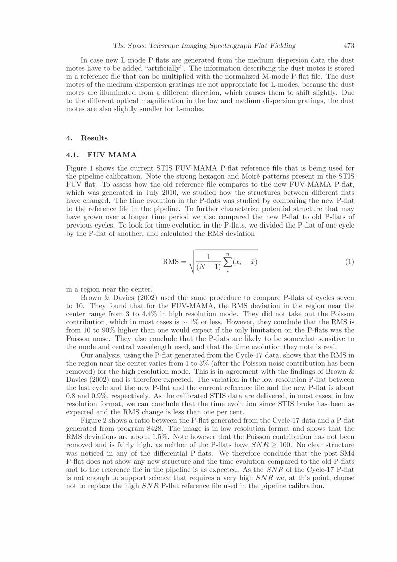
Figure 1 shows the current STIS FUV-MAMA P-flat reference file that is being used forthe pipeline calibration. Note the strong hexagon and Moire patterns present in the STISFUV flat. To assess how the old reference file compares to the new FUV-MAMA P-flat,which was generated in July 2010, we studied how the structures between di!erent flatshave changed. The time evolution in the P-flats was studied by comparing the new P-flatto the reference file in the pipeline. To further characterize potential structure that mayhave grown over a longer time period we also compared the new P-flat to old P-flats ofprevious cycles. To look for time evolution in the P-flats, we divided the P-flat of one cycleby the P-flat of another, and calculated the RMS deviation

RMS =

!

"

"

#

1

(N ! 1)

n$

i

(xi ! x) (1)

in a region near the center.Brown & Davies (2002) used the same procedure to compare P-flats of cycles seven

to 10. They found that for the FUV-MAMA, the RMS deviation in the region near thecenter range from 3 to 4.4% in high resolution mode. They did not take out the Poissoncontribution, which in most cases is " 1% or less. However, they conclude that the RMS isfrom 10 to 90% higher than one would expect if the only limitation on the P-flats was thePoisson noise. They also conclude that the P-flats are likely to be somewhat sensitive tothe mode and central wavelength used, and that the time evolution they note is real.

Our analysis, using the P-flat generated from the Cycle-17 data, shows that the RMS inthe region near the center varies from 1 to 3% (after the Poisson noise contribution has beenremoved) for the high resolution mode. This is in agreement with the findings of Brown &Davies (2002) and is therefore expected. The variation in the low resolution P-flat betweenthe last cycle and the new P-flat and the current reference file and the new P-flat is about0.8 and 0.9%, respectively. As the calibrated STIS data are delivered, in most cases, in lowresolution format, we can conclude that the time evolution since STIS broke has been asexpected and the RMS change is less than one per cent.

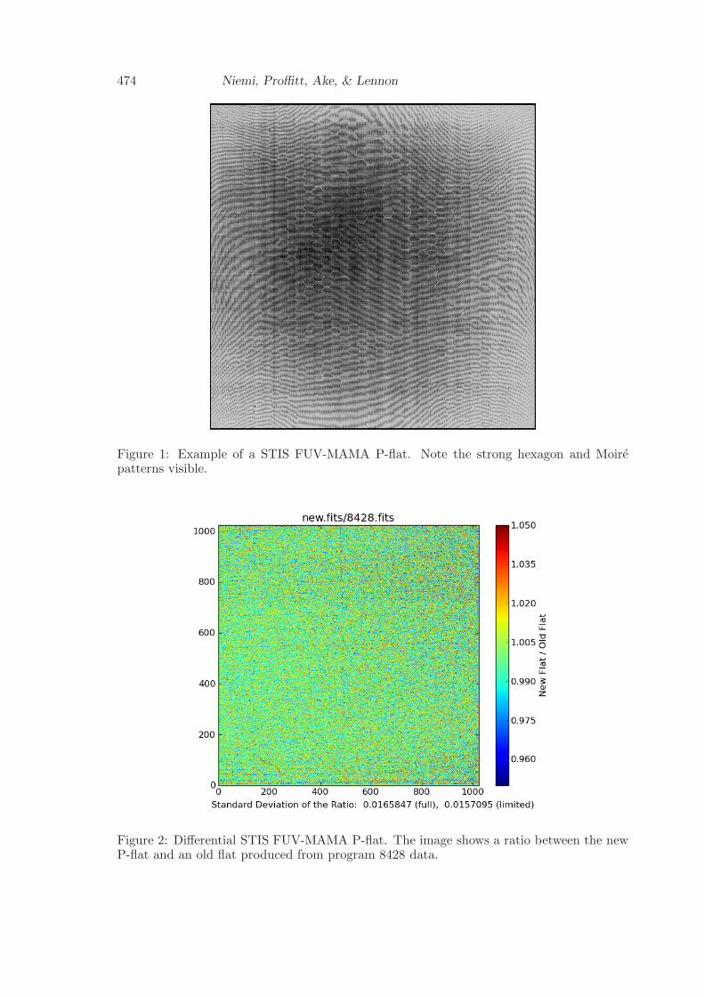
Figure 2 shows a ratio between the P-flat generated from the Cycle-17 data and a P-flatgenerated from program 8428. The image is in low resolution format and shows that theRMS deviations are about 1.5%. Note however that the Poisson contribution has not beenremoved and is fairly high, as neither of the P-flats have SNR # 100. No clear structurewas noticed in any of the di!erential P-flats. We therefore conclude that the post-SM4P-flat does not show any new structure and the time evolution compared to the old P-flatsand to the reference file in the pipeline is as expected. As the SNR of the Cycle-17 P-flatis not enough to support science that requires a very high SNR we, at this point, choosenot to replace the high SNR P-flat reference file used in the pipeline calibration.


Figure 1: Example of a STIS FUV-MAMA P-flat. Note the strong hexagon and Moirepatterns visible.

Figure 2: Di!erential STIS FUV-MAMA P-flat. The image shows a ratio between the newP-flat and an old flat produced from program 8428 data.


Figure 3: Example of a STIS NUV-MAMA P-flat. Note the strong Moire pattern presentand the vignetted corners.

4.2. NUV MAMA

We do not yet have an estimate for the time evolution in the NUV flat, as we are still in theprocess of obtaining Cycle-17 data. However, a new P-flat will be generated from Cycle-17 data as soon as the data become available and it will be compared to the reference filecurrently in the pipeline, as well as, to the old reference files. Since the FUV-MAMA did notshow any structural changes, we do not expect major time evolution in the NUV-MAMAflat field structure either.

4.3. CCD

New STIS CCD P-flats (see Fig. 4) were produced in November 2009 after which wethoroughly tested them. For testing the new P-flats we used post-SM4 data (GO proposal11567, P.I. Pro!tt) that were taken with the G230MB grating through a long slit 52! 0.2.This data set is well suited for testing as these data are of high signal-to-noise (SNR " 300)and moreover these observations were dithered along the slit. The observations used areof variable stars of beta Cep type (HD024760 and HD109668). There does not appear tobe any detectable photometric or velocity variation between the individual exposures. The1-dimensional extracted spectral stripes, which are all of the same target, had been recordedon di"erent places on the detector and should therefore tell us readily if the P-flat correctionis appropriate by minimizing the scatter between the spectra at di"erent detector positions.We also compared the extracted 1-dimensional spectra (1dx) that were calibrated with thenew P-flat to a situation where no flat fielding was performed to assess whether the P-flatcan improve the signal-to-noise ratio of the data or not, and to ensure that the P-flat doesnot generate any spurious features.


Figure 4: Example of a STIS CCD P-flat. The dust motes and small scale blemishes havebeen marked with red circles.

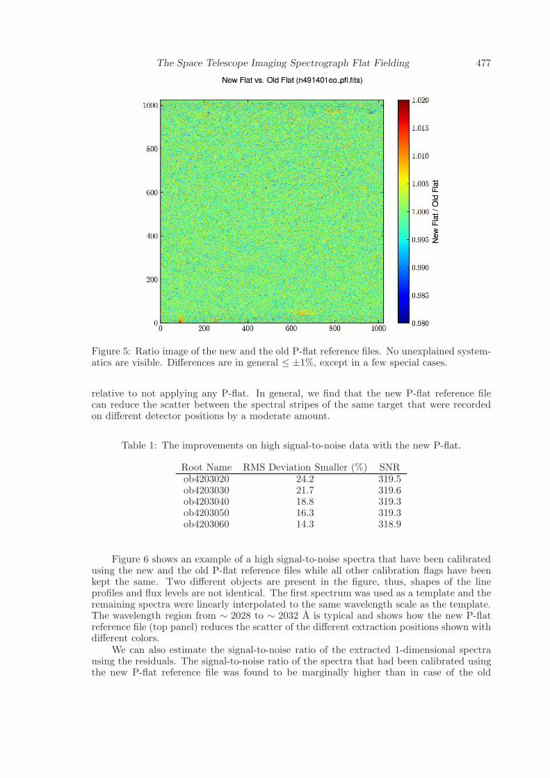
Figure 5 shows a ratio between the new and the old P-flat based on data taken in 2003.No systematic di!erences are noted in the ratio image and the di!erences are in general lessthan ±1%. We also made a ratio image of the new and the old error arrays to assess thesignal-to-noise ratio of the new P-flat. The new P-flat was found to have slightly (in generalwithin few %) larger errors across the detector. This di!erence is due to the number of files,i.e. the number of electrons recorded, used to generate the new P-flat, which is slightly lowerthan for the old P-flat. Even so, the signal-to-noise ratio of the new P-flat is high enoughso that it can be used for high signal-to-noise data without degrading the data quality.

As no systematic and unexplainable di!erences between the old and the new P-flat werenoted, we tested the new P-flat on high signal-to-noise post-SM4 data. Because no accuratestellar models are available for HD024760 or HD109668, we used the spectrum observed atthe last dither position as a template for the testing. All values quoted are always withrespect to the template spectrum so only relative di!erences should be compared.

The new P-flats can reduce the residual scatter and the RMS deviation up to ! 22%in comparison to the old reference files when high signal-to-noise ratio spectra recorded atdi!erent dither positions are compared. No spurious features were detected when the newP-flats were used. The new P-flat was found to have only a modest impact on the signal-to-noise ratio of the extracted 1-dimensional spectra; adopting the new P-flat improved thesignal-to-noise ratio of the extracted spectra " 1% compared to the old P-flat or if no flatfielding was applied. The improvements on high signal-to-noise data range from modestto moderate, numerical values are listed in Table 1. The RMS deviation in extracted 1-dimensional spectra (x1d) is from ! 14 to up to ! 24% smaller in case of the spectra thatwere calibrated using the new P-flat instead of the old reference file. The RMS deviationwas found to be from ! 5 to ! 19% smaller when extracted 1-d spectra were calibrated withthe new P-flat in comparison to the situation where no flat fielding was performed. Thus,it was found that the old P-flat, in case of post-SM4 data, actually increased the scatter


Figure 5: Ratio image of the new and the old P-flat reference files. No unexplained system-atics are visible. Di!erences are in general ! ±1%, except in a few special cases.

relative to not applying any P-flat. In general, we find that the new P-flat reference filecan reduce the scatter between the spectral stripes of the same target that were recordedon di!erent detector positions by a moderate amount.

Table 1: The improvements on high signal-to-noise data with the new P-flat.

Root Name RMS Deviation Smaller (%) SNRob4203020 24.2 319.5ob4203030 21.7 319.6ob4203040 18.8 319.3ob4203050 16.3 319.3ob4203060 14.3 318.9

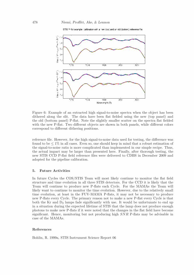
Figure 6 shows an example of a high signal-to-noise spectra that have been calibratedusing the new and the old P-flat reference files while all other calibration flags have beenkept the same. Two di!erent objects are present in the figure, thus, shapes of the lineprofiles and flux levels are not identical. The first spectrum was used as a template and theremaining spectra were linearly interpolated to the same wavelength scale as the template.The wavelength region from " 2028 to " 2032 A is typical and shows how the new P-flatreference file (top panel) reduces the scatter of the di!erent extraction positions shown withdi!erent colors.

We can also estimate the signal-to-noise ratio of the extracted 1-dimensional spectrausing the residuals. The signal-to-noise ratio of the spectra that had been calibrated usingthe new P-flat reference file was found to be marginally higher than in case of the old


Figure 6: Example of an extracted high signal-to-noise spectra when the object has beendithered along the slit. The data have been flat fielded using the new (top panel) andthe old (bottom panel) P-flat. Note the slightly smaller scatter on the spectra flat fieldedwith the new P-flat. Two di!erent objects are shown in both panels, while di!erent colorscorrespond to di!erent dithering positions.

reference file. However, for the high signal-to-noise data used for testing, the di!erence wasfound to be ! 1% in all cases. Even so, one should keep in mind that a robust estimation ofthe signal-to-noise ratio is more complicated than implemented in our simple recipe. Thus,the actual impact may be larger than presented here. Finally, after thorough testing, thenew STIS CCD P-flat field reference files were delivered to CDBS in December 2009 andadopted for the pipeline calibration.

5. Future Activities

In future Cycles the COS/STIS Team will most likely continue to monitor the flat fieldstructure and time evolution in all three STIS detectors. For the CCD it is likely that theTeam will continue to produce new P-flats each Cycle. For the MAMAs the Team willlikely want to continue to monitor the time evolution. However, due to the relatively smalltime evolution, at least in the FUV-MAMA P-flats, it may not be necessary to producenew P-flats every Cycle. The primary reason not to make a new P-flat every Cycle is thatboth the Kr and D2 lamps fade significantly with use. It would be unfortunate to end upin a situation during the expected lifetime of STIS that the lamp does not produce enoughphotons to make new P-flats if it were noted that the changes in the flat field have becomesignificant. Hence, monitoring but not producing high SNR P-flats may be advisable incase of the MAMAs.

References

Bohlin, R. 1999a, STIS Instrument Science Report 06


Bohlin, R. 1999b, STIS Instrument Science Report 04

Brown T. M. & Davies J. E. 2002, STIS Technical Istrument Report 03

Niemi, S.-M. 2010, STIS Technical Instrument Report 01

Shawn, D., Kaiser M. E. & Ferguson, H. 1998, STIS Instrument Science Report 15

the space telescope imaging spectrograph flat fieldingins/2010calworkshop/niemi.pdf · the space...

Documents