University of South FloridaScholar Commons

Graduate Theses and Dissertations Graduate School

12-8-2005

The Solubility of Triton X-114 and Tergitol 15-S-9in High-Pressure Carbon Dioxide SolutionsBrandon SmeltzerUniversity of South Florida

Follow this and additional works at: http://scholarcommons.usf.edu/etd

Part of the American Studies Commons

This Thesis is brought to you for free and open access by the Graduate School at Scholar Commons. It has been accepted for inclusion in GraduateTheses and Dissertations by an authorized administrator of Scholar Commons. For more information, please contact scholarcommons@usf.edu.

Scholar Commons CitationSmeltzer, Brandon, "The Solubility of Triton X-114 and Tergitol 15-S-9 in High-Pressure Carbon Dioxide Solutions" (2005). GraduateTheses and Dissertations.http://scholarcommons.usf.edu/etd/3825

The Solubility of Triton X-114 and Tergitol 15-S-9 in High-Pressure Carbon Dioxide

Solutions

by

Brandon Smeltzer

A thesis submitted in partial fulfillmentof the requirements for the degree of

Master of Science in Chemical EngineeringDepartment of Chemical Engineering

College of EngineeringUniversity of South Florida

Major Professor: Aydin K. Sunol, Ph.D.Sermin G. Sunol, Ph.D.

Carl J. Biver, Ph.D.

Date of Approval:December 8, 2005

Keywords: cloud point, phase, supercritical, surfactant, template

© Copyright 2006, Brandon Smeltzer

Dedication

I dedicate this work to my family for teaching me the power of a college

education. Thanks for believing in me and making me believe in myself.

Acknowledgments

There are several people I am thankful to for being able to do this research. First

and foremost I must thank Dr. Aydin Sunol for the opportunity to do research. Dr.

Sunol’s guidance has made my research experience very rewarding. I would like to

thank Dr. Sermin Sunol for teaching me how to research previously published works for

relevant information. I would also like to thank Raquel Carvallo for answering an

endless number of questions regarding experimental setups and modeling. Raquel was

also nice enough to extend her library privileges to me to assist my background research.

I would like to thank Haitao Li for letting me use the syringe pump for as long as

necessary to conduct experiments. I owe a debt of gratitude to Naveed Aslam for his

assistance in modeling my systems with his MATLAB program for the PRSV equation of

state with WS mixing rules.

i

Table of Contents

List of Tables iii

List of Figures iv

List of Equations vi

List of Symbols xiii

Abstract xvii

Chapter 1 Introduction 1

Chapter 2 Background and Theory 52.1 A Historical Perspective of the Supercritical Phenomena 52.2 Surfactants 62.3 Supercritical Solubility Determination Methods 112.4 Published Works on Surfactant Solubility in Supercritical Carbon

Dioxide 152.5 Entrainer Solubility in Supercritical Carbon Dioxide 17

Chapter 3 Phase Equilibrium Modeling 193.1 Phase Equilibrium 193.2 Excess Functions 223.3 Liquid-Liquid Equilibrium, Vapor-Liquid Equilibrium, and Liquid-

Liquid-Vapor Equilibrium 233.4 Activity Coefficient Models 323.5 The Model 413.6 Critical Property Estimation 483.7 Phase Behavior Classification 50

Chapter 4 Experimental 534.1 Equipment 534.2 Experimental Set-Up 624.3 Procedure and Materials 634.4 Clean-Up 64

ii

Chapter 5 Results and Discussion 675.1 A Comparison of the Improved Rackett Equation to the PRSV

Equation 675.2 Critical Property Estimation of Surfactants 705.3 Carbon Dioxide and Surfactant Binary Systems 705.4 Carbon Dioxide-Ethanol-Triton X-114 Ternary System 715.5 Carbon Dioxide-Ethanol-Tergitol 15-S-9 Ternary System 735.6 Error Introduction 74

Chapter 6 Conclusions, Recommendations, and Future Directions 786.1 Conclusions 786.2 Recommendations 796.3 Future Directions 81

References 83

Appendices 86Appendix A Chemical MSDS 87Appendix B IRE and PRSV Comparison 109Appendix C Critical Property Estimation 111Appendix D Sample Calculations 116

iii

List of Tables

Table 1. Critical Properties of Surfactants 70

Table 2. Ternary Mixture Compositions Studied with Triton X-114 71

Table 3. Observed Cloud Point Pressures of Triton X-114 Mixtures 71

Table 4. Standard Deviations of Cloud Point Pressure Measurements 72

Table 5. Ternary Mixture Compositions Studied with Tergitol 15-S-9 73

Table 6. Observed Cloud Point Pressures of Tergitol 15-S-9 Mixtures 73

Table 7. Standard Deviations of Cloud Point Pressure Measurements 74

Table 8. Carbon Dioxide Liquid Molar Volume Calculation Comparison 110

Table 9. Joback Group Contribution Factors for Triton X-114 111

Table 10. Joback Group Contribution Factors for Tergitol 15-S-9 112

iv

List of Figures

Figure 1. Normal Micelle Formation/Reverse Micelle Formation 10

Figure 2. Dynamic Experimental Set-Up 12

Figure 3. Static Experimental Set-Up 13

Figure 4. Phase Behavior of Carbon Dioxide-Ethanol 18

Figure 5. Algorithm for Isothermal Flash Calculations 30

Figure 6. Algorithm for LLV Isothermal Flash Calculations 31

Figure 7. NRTL Activity Coefficient Dependence on α12 Value 36

Figure 8. Phase Behavior Classifications 52

Figure 9. SPM20 Super Phase Monitor 54

Figure 10. The Solubility Cell 55

Figure 11. Fixed Frit Setting 56

Figure 12. Movable Frit Setting 57

Figure 13. SPM20 Super Phase Monitor Controller 58

Figure 14. ISCO 100DX Syringe Pump 59

Figure 15. Lauda Ecoline Low-Temperature Thermostat RE-120 60

Figure 16. ISCO 100DX Syringe Pump Cooling Jacket Set-Up 61

Figure 17. Experimental Set-Up 62

Figure 18. Molar Volume Comparison 68

Figure 19. Error Comparison of the Improved Rackett Equation and the PRSV 69

v

Figure 20. P-x Diagram of Triton X-114 in Carbon Dioxide-Ethanol 72

Figure 21. P-x Diagram of Tergitol 15-S-9 in Carbon Dioxide-Ethanol 74

vi

List of Equations

Equation 1. Gibbs-Duhem Equation 19

Equation 2. Gibbs-Duhem Equation at Constant Pressure and Temperature 19

Equation 3. Gibbs Free Energy at Equilibrium Involving the Distribution ofComponents Between Two Phases at Constant Pressure andTemperature 19

Equation 4. Simplification of Gibbs Free Energy at Equilibrium Involving theDistribution of Components Between Two Phases at ConstantPressure and Temperature 20

Equation 5. Equality of Chemical Potentials of All Species at Equilibrium 20

Equation 6. Chemical Potential of Species 20

Equation 7. Ideal Gas Equation 20

Equation 8. Chemical Potential of a Species at Ideal Gas Conditions 20

Equation 9. Chemical Potential of a Species as a Function of Fugacity 20

Equation 10. Change in Chemical Potential at Isothermal Conditions 21

Equation 11. Change in Chemical Potential of Component 1 in Two-PhaseEquilibrium 21

Equation 12. Change in Chemical Potential of Component 2 in Two-PhaseEquilibrium 21

Equation 13. Equality of Standard States of Chemical Potential in Two-PhaseEquilibrium 21

Equation 14. Equality of Standard States of Fugacities in Two-PhaseEquilibrium 21

Equation 15. Equality of Fugacity of Species in Two Phases 21

vii

Equation 16. Fugacity Coefficient 21

Equation 17. Fugacity Coefficient for a Pure Substance 22

Equation 18. Excess Gibbs Energy 22

Equation 19. Maxwell Relationship for Excess Entropy 22

Equation 20. Maxwell Relationship for Excess Enthalpy 22

Equation 21. Maxwell Relationship for Excess Volume 22

Equation 22. Gibbs-Duhem Equation in Terms of Excess Functions 23

Equation 23. Gibbs-Duhem Equation in Terms of Excess Functions atEquilibrium 23

Equation 24. Gibbs Energy of Mixing for Liquid-Liquid Miscibility 23

Equation 25. Derivative of Gibbs Energy of Mixing for Liquid-LiquidMiscibility 23

Equation 26. Volume Change in Mixing 24

Equation 27. Equality of Fugacities of Component 1 in Liquid-Liquid Mixture 25

Equation 28. Equality of Fugacities of Component 2 in a Liquid-Liquid Mixture 25

Equation 29. Activity Coefficient Equation 25

Equation 30. Activity Coefficient Equation at the Standard State 25

Equation 31. Equality of Fugacities in Vapor and Liquid Phase 26

Equation 32. Fugacity Equality During Vapor-Liquid Equilibrium 26

Equation 33. Distribution Coefficient 26

Equation 34. Distribution Coefficient at Ideal Gas Conditions 26

Equation 35. Distribution Coefficient of Non-Ideal Systems 27

Equation 36. Individual Component Material Balance for Isothermal FlashConditions 27

viii

Equation 37. Material Balance for Vapor Phase at Isothermal Flash Condtions 27

Equation 38. Material Balance for All Components at Isothermal FlashConditions 27

Equation 39. LLVE Material Balance 27

Equation 40. Distribution Coefficient in First Liquid Phase 28

Equation 41. Distribution Coefficient in Second Liquid Phase 28

Equation 42. Molar Fraction of First Liquid Phase 28

Equation 43. Non-linear Equation to Determine Molar Fraction of First LiquidPhase 28

Equation 44. Non-linear Equation to Determine Vapor to Feed Ratio, β 28

Equation 45. Total Mols of Liquid 1 Phase 28

Equation 46. Total Mols of Liquid 2 Phase 28

Equation 47. Vapor Phase Composition of LLVE Isothermal Flash 28

Equation 48. Composition of Liquid 1 Phase of LLVE Isothermal Flash 29

Equation 49. Composition of Liquid 2 Phase of LLVE Isothermal Flash 29

Equation 50. Excess Gibbs Energy for van Laar Activity Coefficient Model 32

Equation 51. Activity Coefficient of Component 1 Using van Laar ActivityCoefficient Model 32

Equation 52. Activity Coefficient of Component 2 Using van Laar ActivityCoefficient Model 32

Equation 53. Parameter A in van Laar Activity Coefficient Model 32

Equation 54. Parameter B in van Laar Activity Coefficient Model 32

Equation 55. Activity Coefficient of Component 1 Using Regular SolutionsTheory 33

Equation 56. Activity Coefficient of Component 2 Using Regular SolutionsTheory 33

ix

Equation 57. Volume Fraction of Component 1 in Regular Solutions Theory 34

Equation 58. Volume Fraction of Component 2 in Regular Solutions Theory 34

Equation 59. Excess Gibbs Energy Using Wilson Equation 34

Equation 60. Activity Coefficient of Component 1 Using Wilson Equation 34

Equation 61. Activity Coefficient of Component 2 Using Wilson Equation 34

Equation 62. Λ12 parameter of Wilson Equation 35

Equation 63. Λ21 parameter of Wilson Equation 35

Equation 64. Gibbs Energy of Cell 1 in NRTL Activity Coefficient Model 35

Equation 65. Gibbs Energy of Cell 2 in NRTL Activity Coefficient Model 35

Equation 66. Excess Gibbs Energy of Cells in NRTL Activity CoefficientModel 35

Equation 67. Ratio of Local Mole Fraction x21 to x11 in NRTL ActivityCoefficient Model 36

Equation 68. Ratio of Local Mole Fraction x12 to x22 in NRTL ActivityCoefficient Model 36

Equation 69. Local Mole Fraction x21 in NRTL Activity Coefficient Model 37

Equation 70. Local Mole Fraction x12 in NRTL Activity Coefficient Model 37

Equation 71. Excess Gibbs Energy of Mixture in NRTL Activity CoefficientModel 37

Equation 72. Dimensionless Local Interaction Energy Parameter τ21 for NRTLActivity Coefficient Model 37

Equation 73. Dimensionless Local Interaction Energy Parameter τ12 for NRTLActivity Coefficient Model 37

Equation 74. Dimensionless Non-randomness Interaction Energy ParameterG21 for NRTL Activity Coefficient Model 37

Equation 75. Dimensionless Non-randomness Interaction Energy ParameterG12 for NRTL Activity Coefficient Model 37

x

Equation 76. Activity Coefficient of Component 1 Using NRTL ActivityCoefficient Model 38

Equation 77. Activity Coefficient of Component 2 Using NRTL ActivityCoefficient Model 38

Equation 78. Total Excess Gibbs Energy Using UNIQUAC Activity CoefficientModel 38

Equation 79. Combinatorial Excess Gibbs Energy Using UNIQUAC ActivityCoefficient Model 39

Equation 80. Segment Fraction for UNIQUAC Activity Coefficient Model 39

Equation 81. Area Fraction for UNIQUAC Activity Coefficient Model 39

Equation 82. Residual Excess Gibbs Energy Using UNIQUAC ActivityCoefficient Model 39

Equation 83. Molecule Segment Energy Difference τji Dimensionless Parameter 39

Equation 84. Activity Coefficient Equation for UNIFAC Activity CoefficientModel 40

Equation 85. Combinatorial Activity Coefficient for UNIFAC ActivityCoefficient Model 40

Equation 86. Surface Area and Volume Parameter Relationship Using UNIFACActivity Coefficient Model 41

Equation 87. Residual Activity Coefficient for UNIFAC Activity CoefficientModel 41

Equation 88. Residual Group Activity Coefficient for UNIFAC ActivityCoefficient Model 41

Equation 89. Molecule Segment Interaction Energy Parameter 41

Equation 90. Peng-Robinson Equation of State 42

Equation 91. Peng-Robinson-Stryjek-Vera (PRSV) Equation of State 42

Equation 92. Compressibility Factor 42

Equation 93. Cubic Form of PRSV Equation of State 42

xi

Equation 94. Dimensionless Attractive Force Correction of PRSV 42

Equation 95. Dimensionless Repulsive Force Correction of PRSV 42

Equation 96. Repulsive Force Correction of PRSV 43

Equation 97. Attractive Force Correction of PRSV 43

Equation 98. -Dimensionless Function of Reduced Temperature 43

Equation 99. PRSV Constant Characteristic of a Substance 43

Equation 100. Acentric Factor Function 44

Equation 101. Reduced Temperature Equation 44

Equation 102. Excess Helmholtz Energy at Infinite Pressure Relationship toExcess Gibbs Energy 44

Equation 103. Wong-Sandler Mixing Rule for a Mixture 44

Equation 104. Wong-Sandler Mixing Rule for ij Component 44

Equation 105. Repulsive Force Correction of Mixture by Wong-Sandler MixingRules 45

Equation 106. Attractive Force Correction of Mixture by Wong-Sandler MixingRules 45

Equation 107. Excess Gibbs Energy Relationship to Activity Coefficients 45

Equation 108 Fugacity Coefficient 45

Equation 109. Vapor Mole Fraction Equation 45

Equation 110. Wagner Equation for Ethanol Vapor Pressure 46

Equation 111. Reduced Temperature Parameter of Wagner Equation 46

Equation 112. Poynting Factor 46

Equation 113. Rackett Equation 46

Equation 114. Critical Compressibility Factor 46

xii

Equation 115. Mole Fraction Balance 46

Equation 116. Vapor Phase Mole Balance 47

Equation 117. Improved Rackett Equation 47

Equation 118. Critical Temperature Estimation Using Joback Method 49

Equation 119. Critical Pressure Estimation Using Joback Method 49

Equation 120. Critical Volume Estimation Using Joback Method 49

Equation 121. Acentric Factor 49

xiii

List of Symbols

Notation

a, b PRSV equation of state parameters

a Activity of species

a Equation of state “energy” parameter (for Wong-Sandler mixing rules)

b Equation of state “excluded” volume parameter (for Wong-Sandler mixing rules)

A, B Dimensionless terms in PRSV Equation of State

A, B Van Laar Activity Coefficient Parameters

C Constant for Wong-Sandler Mixing Rules

f Fugacity (bar)

F Feed (mol/time)

g Gibbs energy (J/mol)

G Gibbs energy (J/mol)

H Enthalpy (J/mol)

k Binary interaction coefficient (for Wong-Sandler mixing rules)

K VLE ratio

l Volume to surface area ratio

n Number of atoms in a molecule

P Pressure of mixture, bar

q Surface factor

xiv

r Volume factor

R Universal Gas Constant

S Entropy (J/mol K)

T Temperature of mixture, K

u Average interaction energy (J/mol)

U Interaction energy (J/mol)

V Molar volume, cm3/mol

x Liquid mole fractions

y Vapor mole fractions

z Coodination number

z Mole fraction in feed

Z Compressibility factor

Greek Letters

Function of acentric factor and the reduced temperature

Β Ratio of vapor to feed

Γ Activity coefficient

Δ Change in a property of a component

γ Activity coefficient

δ Solubility parameter

θ Area fraction of a species

Λ Wilson equation activity coefficient parameter

0 Function of acentric factor

xv

μ Chemical potential

ν Molar volume

ν Number of groups in mixture

τ Unitless energy difference parameter for UNIQUAC Model

τ Reduced temperature ratio

Fugacity coefficient

ψ Unitless energy difference parameter or UNIFAC Model

Acentric factor

Subscript

0 Pure component property

b Boiling point

c Critical property

i Component in mixture

j Component in mixture

m Molar volume

mix Mixture property

P Pressure

r Reduced property

RA Rackett equation parameter

T Temperature

x Mole Fraction

xvi

Superscript

0 Pure component property

Infinite dilution

α One component in mixture

β One component in mixture

c Critical property

C Combination

E Excess property

ex Excess property

k Component of mixture

L Liquid phase

R Residual

sat Saturation condition

V Vapor phase

xvii

The Solubility of Triton X-114 and Tergitol 15-S-9 in High-Pressure Carbon

Dioxide Solutions

Brandon Smeltzer

ABSTRACT

In the sol gel production of high surface area catalyst, the template, a surfactant, is

the key component of the process. A template too soluble in the supercritical drying-

extraction process can yield a catalyst with a lower surface area. A template completely

insoluble in the supercritical drying-extraction process can lead to a longer calcinations

step and lower catalyst surface area. Template recovery also enhances the economic

feasibility of plant scale production of high surface area catalyst. For these reasons

knowing surfactant solubility in supercritical media is important.

The solubility of surfactants tert-octylphenoxypolyethoxyethanol (commercially

available and hereafter referred to as Triton X-114) and alkyloxypolyethyleneoxyethanol

(commercially available and hereafter referred to as Tergitol 15-S-9) in supercritical

carbon dioxide and ethanol entrainer have been determined at five-degree increments

from 35oC to 50oC. The solubility of the surfactants was determined by charging a

variable volume cloud point system with the entrainer-surfactant mixture followed by

liquid carbon dioxide. With the resulting stirred homogeneous mixture heated to

temperature, cloud point pressures were observed as the phase analyzer cell was

pressurized by adjusting the variable volume. An average of five values for cloud point

xviii

pressure is reported here. The mixture behaviors were modeled using the Improved

Rackett equation and the Peng-Robinson-Stryjek-Vera (PRSV) equation of state with

Wong-Sandler (WS) mixing rules.

For the Carbon Dioxide (CO2) (1) – Ethanol/Triton X-114 (2) mixtures studied,

compositions ranged from 93.2 mol% CO2 to 97.7 mol% CO2. The solubility of Triton

X-114 ranged from 0.02 mol% to 0.05 mol% at temperatures ranging from 35oC to 50oC.

Cloud point pressures observed for this system range from 95 bar to 143 bar.

For the CO2 (1) – Ethanol/Tergitol 15-S-9 (2) mixtures studied, compositions

ranged from 92.3 mol% CO2 to 94.4 mol % CO2 . The solubility of Tergitol 15-S-9

ranged from 0.02 mol% to 0.03 mol% at temperatures ranging from 35oC to 50oC. Cloud

point pressures observed for this system range from 89 to 154 bar.

1

Chapter 1

Introduction

Supercritical fluids possess interesting and industry applicable characteristics that

set them apart from typical solvents. The lack of surface tension, the mobility of a gas,

and the solvation power of a liquid are three unique properties that make supercritical

fluids very attractive as tunable solvents (15.McHugh & Krukonis 1986). Supercritical

fluids can be used for the selective recovery of solutes by adjusting pressure and

temperature.

One engineering field where selective solute recovery can have a major economic

impact is novel catalyst design. One of the key components in porous aerogel catalyst

production is the template - a surfactant, in this case tert-octylphenoxypolyethoxyethanol

(commercially available as Triton X-114) and alkyloxypolyethyleneoxyethanol

(commercially available as Tergitol 15-S-9). A template too soluble in a supercritical

fluid will be removed too easily from the porous catalyst structure and result in collapsed

pores. Too many collapsed pores yield a catalyst with a low surface area. A template

completely insoluble in a supercritical fluid will not be removed until a calcination

process. A template completely insoluble in a supercritical fluid is harmful in catalyst

synthesis because the calcination process may have to be extended to allow for the

template to breakdown.

2

For these reasons, the solubility of the surfactants Triton X-114 and Tergitol 15-

S-9 in supercritical carbon dioxide is important. Efficient template recovery with

recyclable supercritical carbon dioxide can bring the plant scale production of porous

catalyst closer to reality with the improvement of economic feasibility.

To acquire the important surfactant solubility data two different experimental

methods can be employed, a static experimental set-up or a dynamic experimental set-up.

The static experimental set-up can yield P-T-x data. The dynamic experimental set-up

can yield P-T-x-y data (4.Dieters & Schneider 1986). The static experimental set-up

works quite well for liquid or solid solubility experiments, particularly when data is

needed quickly. The dynamic experimental set-up is most useful for solid solubility

determination. The dynamic experimental set-up is not necessarily a good choice for

liquid solubility experiments for a few reasons: the supercritical solvent can push the

liquid of interest out of the solubility cell without solubilizing it; phase changes can go

undetected; the solubility of the supercritical solvent in the liquid of interest cannot be

measured; experimental set-ups for multi-component mixtures may require a more

elaborate design to ensure that the components of the mixture are not improperly

removed during the experimental run (15.McHugh & Krukonis 1986).

In the static (also called synthetic) experimental set-up, known amounts of

substances are transferred into the solubility cell. The mixture composition is then

determined from the initial conditions. The solubility cell is then brought up to the

experimental temperature and pressurized until a homogeneous phase is observed. Data

that can be ascertained from a static experimental set-up include P-x diagrams and T-x

diagrams. One aspect of the static experimental set-up that researchers favor is the ability

3

to get solubility data at various temperatures with just one experimental run. Conversely,

the static experimental set-up is not favorable to researchers when vapor-liquid

equilibrium (VLE) data is needed (4.Deiters & Schneider 1986).

In the dynamic (also called analytical) experimental set-up the supercritical

solvent flows at a set temperature and pressure through a solubility cell containing a

known amount of the solute of interest. The resulting mixture then flows through an

analytical device (a spectrometer – UV/Vis or IR, a gas chromatogram, or mass

spectrometer) and a collection chamber. Solute solubility is then determined by

interpreting the chromatograph and comparing it with the mass of solute recovered from

the collection chamber. Data that can be ascertained from the dynamic experimental set-

up include P-x-y diagrams and T-x-y diagrams (4.Deiters & Schneider 1986). The

dynamic experimental set-up that appeals to the researcher because: data can be acquired

rapidly, the experiments are easily reproducible, and for most cases the sampling

mechanism is fairly simple (15.McHugh & Krukonis 1986).

The following chapters will explain the background theory to the experiments,

the experimental set-up and procedure, and finally the results, discussions, and future

directions where this research can be applied.

Chapter 2 will further discuss the specific details of component solubility in

supercritical media, particularly carbon dioxide. A discussion of surfactants and their

properties will be presented here as well. The two methods for solubility determination

in supercritical fluids will be discussed. Previously published work on surfactant

solubility in supercritical fluids will be presented. A discussion on the solubility of

ethanol in supercritical carbon dioxide will be presented.

4

Chapter 3 will discuss phase equilibrium. The focus of the phase equilibrium

discussion will be liquid-liquid equilibrium, vapor-liquid equilibrium, liquid-liquid-vapor

equilibrium and the models used to describe them.

Chapter 4 will discuss the experimental set-up for supercritical solubility

determination and the experimental method used.

Chapter 5 will pertain to the results analysis and discussions of the experiments.

Data will be presented in table and graph form.

Chapter 6 is dedicated to conclusions and the future directions that directly

involve this research.

5

Chapter 2

Background and Theory

The purpose of this chapter is to explain several things: the supercritical

phenomenon, surfactant properties, some ways supercritical solubility can be determined,

published works on surfactant solubility in supercritical carbon dioxide, and the solubility

of ethanol in supercritical carbon dioxide.

2.1 A Historical Perspective of the Supercritical Phenomena

Supercritical fluid technology is a branch of chemical engineering that has been in

use since its discovery in 1822, by Baron Caginard de la Tour. De la Tour conducted

high-pressure experiments involving a flint ball sealed in a cannon barrel with ethanol.

Changes in the sound of the ball hitting the barrel wall were documented and de la Tour

informed the scientific community of what is known as the critical point.

Dr. Thomas Andrews did the first major investigations of carbon dioxide as a

supercritical fluid. Dr. Andrews reported the critical values of carbon dioxide to be

30.92oC and 73 atmospheres (15.McHugh & Krukonis 1986). The values reported by Dr.

Andrews are very close to the accepted published values for carbon dioxide of 31.1oC

and 73.8 bars (21.Prausnitz & Lichtenthaler & Azevedo 1999). In 1879, Hannay and

Hogarth presented their experimental results for the solubility of several inorganic salts in

6

ethanol using a modified version of Dr. Andrews’ experimental set-up. Hannay and

Hogarth concluded that solubility could be pressure dependent.

Gore authored the earliest published paper regarding the use of liquid carbon

dioxide as a solvent in 1861. Gore described liquid carbon dioxide as being a very poor

solvent. Villard investigated the effectiveness of four compounds as supercritical fluids:

carbon dioxide, ethylene, nitrous oxide, and methane in 1896 (15.McHugh & Krukonis

1986).

Alfred W. Francis published one of the most extensive studies concerning the

solvent power of liquid carbon dioxide in 1954. Francis studied the solubility of 261

individual substances with carbon dioxide and constructed ternary diagrams for 464

systems. The temperature range for Francis’ study is 21oC to 26oC with a pressure near

65 atmospheres. The work done by Francis is an excellent starting point for supercritical

separation experiments involving carbon dioxide because a relative effectiveness of

separation can be discerned from his data before an experiment is done (6.Francis 1954).

2.2 Surfactants

Surfactants are a unique class of chemicals in part because of their complex

chemical structures and their resulting physical properties. Surfactant is short hand for

surface-active agent. The highest concentration of a surfactant can be found at the

surface of a solution as compared to the bulk solution. The essential purpose of a

surfactant is to wet a solid surface thus allowing for contact between the solid surface and

another liquid. The contact between the solid surface and another liquid is accomplished

7

because the surfactant actually lowers the surface tension of the liquid, allowing it to

enter areas that would otherwise be blocked to it (20.Porter 1991).

Surfactants belong to a group of chemicals called amphiphiles because they

contain hydrophobic and hydrophilic parts or tails. The hydrophobic tail of a surfactant

is usually a long hydrocarbon chain. The hydrophilic tail of the surfactant is usually a

functional group with a high affinity for water (29.Texter 1999). Scientists have several

different ways to categorize surfactants, which include physical state and ionicity.

The physical state of a surfactant at room temperature has a major influence on

the properties that the surfactant exhibits. The crystalline structure of a surfactant has a

direct effect on the wetting capabilities of the surfactant. Packing can be arranged head

to head and tail to tail or head to tail in monolayers or bilayers. The level to which the

packing is ordered dictates the location of the polar and non-polar heads. Some

surfactants exhibit polymorphism – the ability to have more than one stable crystalline

structure. The solid phases may differ completely in structure at the unit cell level or in a

one-dimensional direction with the stacking of layers (29.Texter 1999).

One of the major differences between crystalline and liquid surfactants at room

temperature is the order within the chemical structure. Crystalline structures can exhibit

long range and short-range order. Liquid surfactants however only exhibit short-range

order. Surfactants that have no long-term order are termed isotropic (29.Texter 1999).

Besides the physical state, another way to classify surfactants is by ionicity.

Ionicity concerns the charge associated with the surfactant. Anionic surfactants have a

negative charge on the long chain. The three most common anionic groups are the

sulfonate (-SO3-), the carboxylate (-CO2

-), and the sulfate(-OSO3-). Arranged according

8

to their hydrophilic tendencies, the carboxylate is the most hydrophilic followed by the

sulfonate, then the sulfate. Anionic surfactants are utilized in a variety of industries

including: paints, textiles, petroleum, household detergents, paper, polishes, shampoos,

personal care soaps, and cosmetics (20.Porter 1991).

Nonionic surfactants contain a head group that has no charge associated with it.

Repeating units of ethylene oxide in the surfactant structure are most common in the

nonionic surfactants. Hydration with nonionic surfactants containing ethylene oxide

groups is believed to occur at a rate of three water molecules for every ethylene oxide

unit. Nonionic surfactants have applications in various industries including: petroleum,

shampoos, textiles, household cleaners, paper, and cosmetics (20.Porter 1991).

Cationic surfactants have a positive charge on the long chain. Cationic

surfactants are a good source of hydrogen bonds. Cationic surfactants are employed in a

plethora of chemical industries including: textiles, biocides, petroleum, hair care,

fertilizers, and lubricants (20.Porter 1991).

Zwitterionic surfactants can carry positive or negative charge depending on the

surrounding conditions. Zwitterionic surfactants are also called ampoterics. Zwitterionic

surfactants have a wide range of applications in various industries including: dish-

washing soap, hand soap, petroleum, textiles, fire fighting, car washing soap, and fabric

softeners (20.Porter 1991).

In addition to the qualitative classification methods applied to surfactants a few

quantitative methods have been developed to aid in process design decisions. Perhaps the

most well known quantitative properties of surfactants are the hydrophile lipophile

balance number (HLB), the critical micelle concentration (CMC), and the Kraft point.

9

Each of these quantitative properties gives great insight into the physical complexities of

surfactants.

The HLB of a surfactant is a measure of effectiveness of a surfactant in water-oil

systems emulsification and is based on the chemical structure of the surfactant. The HLB

is hydrophilic percent of the surfactant in molar concentration divided by five. The scale

goes from zero to twenty. Zero represents a surfactant completely insoluble in water.

Twenty corresponds to a surfactant completely soluble in water. Thus an HLB number of

ten means the surfactant has an equal affinity for water and oil. It should be noted that

the HLB number is a very good for describing the behavior of nonionic surfactants, but it

does not a present a good description for ionic surfactant behavior in water-oil systems

(20.Porter 1991). However modifications have been made to the HLB calculations so it

can be applied successfully to surfactants that carry a charge (29.Texter 1999).

The CMC of a surfactant is the lowest concentration at which a surfactant will

gather together and form micelles – a structured arrangement of surfactant molecules.

Micelles can take the several shapes: cylindrical, bilayers, spherical, vesicles, rodlike,

ellipsoidal, and reverse micelles. When micelles form they function just like bulky

molecules. Normal micelles form when the polar head groups of the surfactant form a

circle with the non-polar tails filling in the circle. Reverse micelles form when the polar

head groups of the surfactants band together with the non-polar tails on the outside of the

circle. Figure 1 shows an illustration of normal micelles and reverse micelles. The size

of the micelles that form depend the number of surfactant molecules involved –called the

aggregate number - in the micelle formation.

10

Figure 1. a). Normal Micelle Formation b). Reverse Micelle Formation (29.Texter1999)

There are several methods available to the researcher to determine the CMC of a

surfactant including: density, refractive index, specific heat, viscosity and x-ray

diffraction (29.Texter 1999).

The chemical structure dictates the CMC of a surfactant. With regard to the

hydrophilic group, the CMC is relatively unaffected by a charged head group. The CMC

of an ethoxylated non-ionic surfactant is lower than a charged hydrophilic group. An

ethylene oxide group addition to a surfactant increases the CMC. The CMC increases

with the inclusion of polar atoms in the hydrophobic group. A decrease in the CMC is

seen when the number of carbons in the hydrophobic group increases (20.Porter 1991).

Closely associated with the CMC of a surfactant is the Kraft point. The Kraft

point is the temperature where the solubility of the surfactant in water is equivalent to the

CMC. Above the Kraft point micelles form easily, whereas below the Kraft point the

surfactant solubility in water is too low for micelle development (29.Texter 1999).

11

2.3 Supercritical Solubility Determination Methods

There are two different methods employed to determine component solubility in a

supercritical fluid - a dynamic method and a static method. Both methods will be

discussed in this section. Benefits and drawbacks for each type of experimental set-up

will be presented.

The dynamic method for component solubility in a supercritical fluid is termed

such because the supercritical fluid is constantly pumped through a cell containing the

solid or liquid of interest. Figure 2 shows a diagram of a dynamic experimental set-up

for solubility determination. An equilibrium cell is charged with a known weight of the

compound of interest. The solvent is pumped into the system at room temperature and

then compressed to the desired operating pressure. The flowing solvent reaches the

desired temperature in the recirculated environment prior to the equilibrium cell. A flow

rate low enough to allow equilibrium between the liquid or solid of interest and the

supercritical solvent is maintained. The equilibrium cell is packed with glass beads

and/or steel wool to ensure that no solute leaves the cell unless it has solubilized into the

supercritical media. The amount of solute in the supercritical fluid can then be

determined by passing the mixture through a UV detector to detect absorbance or by

using a cold trap collector and weighing its contents.

12

Figure 2. Dynamic Experimental Set-Up (15.McHugh & Krukonis 1986)

The dynamic set-up has a few characteristics that make it the method of choice for

the experimenter - a significant amount of solubility data can be ascertained quickly; the

experiments can be reproduced without difficulty; supercritical fluid stripping data can be

accumulated quickly; the set-up can be built in house. The dynamic set-up is not without

constraints however. Clogging, anywhere in the system, with the solute can lead to

inaccurate solubility measurements. Phase changes may occur that go unnoticed in the

equilibrium cell or the piping. The density of the supercritical fluid phase can cause the

supercritical fluid to push the solute out of the equilibrium cell; hence the solubility

measurements will be too high. To offset all of these potential error introductions in

experimental solubility measurements adaptations to the dynamic set-up can be made.

Along with the dynamic set-up for solubility experiments, there is also a static

experimental set-up for solubility determination. The set-up is called static because a

known quantity of the supercritical fluid is pumped into the equilibrium cell. Figure 3

shows a static experimental set-up for solubility determination. In the static set-up, a

13

known weight of solute is put into a variable volume equilibrium cell. The equilibrium

cell is then pumped full of pressurized solvent at ambient temperature. A magnetic stirrer

is used to make the mixture homogeneous. The mixture is heated by an air bath. A

manual pump then pressurizes the mixture until no discernable solute can be observed in

the view cell.

Figure 3. Static Experimental Set-Up (15.McHugh & Krukonis 1986)

The static experimental set-up has several appealing characteristics that make it a

viable route for empirical data collection: phase changes can be visually established;

solubility can be acquired without sampling (UV/Vis or IR detector); pressure and

temperature adjustments can be made easily and quickly. The static set-up however, has

one major constraint - the view cells can fail at higher pressures limiting the pressure

range under which experiments can be conducted (15.McHugh & Krukonis 1986).

14

Variations to the dynamic and static experimental set-ups have been done by

numerous authors to improve experimental accuracy and to increase the type of data that

can be acquired during an experiment. Legret, Richon, and Renon published an

experimental method involving the static experimental set-up allowing for accurate P-T-

x-y measurements in a pressure range of 10-1000 bar and a temperature range of -40oC-

160oC. The authors’ focus for this work centered on sampling the systems at

experimental conditions with a detachable 15µL cell. The 15µL sample cell represented

only 0.015% of the total volume of the solubility cell. The detachable cell is then

connected to a gas chromatograph, vaporized, and analyzed. The method was tested on

the previously studied binary system N2-n-Heptane system to determine the dependability

of the new experimental set-up. As noted by the authors, the most significant aspect of

the experiments is the sample method. Disturbing the phase and thermal equilibrium by

taking a large sample volume will alter the results obtained by the gas chromatograph

(12.Legret & Richon & Renon 1981).

Meskel-Lesavre, Richon, and Renon developed a static experimental set-up in an

effort to eliminate the need for an equation of state entirely. The aforementioned authors’

experimental set-up measures the saturated liquid phase molar volume as well as the

bubble pressure of a mixture directly. The experimental method involves charging the

solubility cell with a known amount of liquid solute which is then cooled to the point of

crystallization under a vacuum. The amount of the gaseous component added to the

system is based on the saturation pressure of the liquid component at the temperature

inside the solubility cell. The cell is then reweighed to determine the amount of gaseous

component added to the solubility cell (16.Meskel-Lesavre & Richon & Renon 1981).

15

Sane, Taylor, Sun, and Thies have developed a semi-continuous flow system with

a microsampler for determining component solubility in supercritical fluids. The authors’

purpose for creating a semi-flow apparatus was due in part to the material whose

solubility was examined – 5,10,15,20-tetrakis(3,5-bis(trifluoromethyl)phenyl)porphyrin

(TBTPP) in supercritical carbon dioxide. The TBTPP was manufactured in house by the

authors. The dynamic experimental set-up for solubility determination was not used

because of the cost and time involved in producing large quantities of TBTPP. The static

experimental set-up was not used due to accuracy issues with spectroscopic analytical

techniques. First, equilibrium between TBTPP and supercritical carbon dioxide is

achieved in a variable volume view cell. Once equilibrium has been achieved, pure,

heated carbon dioxide is supplied to the piston side of the solubility cell by a syringe

pump. This new supply of carbon dioxide pushes the mixture inside the solubility cell

out toward the sample loop. The authors tested the accuracy of the semi-continuous flow

system with phenanthrene-supercritical carbon dioxide experiments and obtained results

comparable to literature values (24.Sane et al. 2004).

2.4 Published Works on Surfactant Solubility in Supercritical Carbon Dioxide

Some studies on the solubility of several surfactants in supercritical carbon

dioxide have been completed and published. Kramer and Thodos have published several

studies on fatty acid surfactant solubility in supercritical carbon dioxide. In 1988,

Kramer and Thodos published data on the solubility of 1-hexadecanol and palmitic acid

in supercritical carbon dioxide from 45oC to 65oC. The authors used a dynamic set-up for

these experiments. Cloud point pressures ranged from 142 bar to 416 bar for the 1-

16

hexadecanol-carbon dioxide system with a solubility range in mole fraction from 0.0019

to 0.0281. Cloud point pressures for the palmitic acid-carbon dioxide system ranged

from 142 bar to 575 bar. The solubility range in mole fraction for this system is 0.00052

to 0.0596 (9.Kramer & Thodos 1988).

In 1989, Kramer and Thodos published data on the solubility of 1-octadecanol

and stearic acid in supercritical carbon dioxide from 45oC to 65oC. Once again, the

authors used a dynamic set-up for these experiments. Cloud point pressures ranged from

140 bar to 453 bar for the 1-octadecanol-carbon dioxide system with a solubility range in

mole fraction from 0.00104 to 0.0319. Cloud point pressures for the stearic acid-carbon

dioxide system ranged from 145 bar to 468 bar. The solubility range in mole fraction for

this system is 0.00079 to 0.0147 (10.Kramer & Thodos 1989).

Keith Consani and Richard Smith did perhaps the most extensive study on

surfactant solubility in supercritical carbon dioxide in 1990. Consani and Smith

conducted solubility experiments on 135 surfactants in supercritical carbon dioxide at

50oC. The authors employed the static experimental set-up for solubility determination

using about one gram of surfactant for each experiment. Perhaps the most significant

feature of this study is the vast number of surfactant categories tested: polyoxylated

compounds, acids, quaternary salts, amines, alkyl phosphates, acid salts, silicon

materials, hydroxy compounds, and miscellaneous surfactants. One other fact that is

important to take notice of is that no entrainer was used in any of the experiments

conducted. Unfortunately, Consani and Smith only conducted the study as a qualitative

analysis reporting solubility as: miscible, partially soluble, and insoluble (3.Consani &

Smith 1990). Nevertheless, the Consani and Smith study can be used in much the same

17

way Francis’ 1954 carbon dioxide study is used as a guide for surfactant solubility in

supercritical carbon dioxide.

Since the publication of the Consani and Smith study on the solubility of several

classes of surfactants, very little published data can be found concerning this area of

research. Liu et al. published a study in 2001, on the solubility of tetraethylene glycol n-

laurel ether in supercritical carbon dioxide with n-pentanol as an entrainer. The authors

used a static experimental set-up to monitor the effects of carbon dioxide density,

entrainer concentration, and increasing pressure on the solubility tetraethylene glycol n-

laurel ether in supercritical carbon dioxide and n-pentanol. Data for cloud point pressure,

mixture density, entrainer concentration, and solubility as weight percentage are

presented for 40oC and 50oC (14.Liu et al. 2001).

In 2003, Liu et al. published a study on the effects of entrainer choice on the

solubility of surfactant Ls-54 in supercritical carbon dioxide. The authors present

solubility data of Ls-54 in supercritical carbon dioxide and Ls-54-entrainer in

supercritical carbon dioxide from 35oC to 50oC. The entrainers tested were 1-propanol,

benzyl alcohol, n-heptanol, and n-pentanol (13.Liu et al. 2003).

2.5 Entrainer Solubility in Supercritical Carbon Dioxide

The choice of entrainer for supercritical solubility experiments can be a tricky

decision for the experimenter to make. The entrainer should be soluble in the

supercritical media, in this case carbon dioxide as well as have the ability to solubilize the

third substrate. A very common choice for entrainer is ethanol. Therefore, knowledge of

the solubility of ethanol in supercritical carbon dioxide is important.

18

In his 1954 publication, Francis reported ethanol to be miscible with carbon

dioxide. Recall that the conditions for Francis’ experiments were a temperature of 21oC

to 26oC and a pressure at about 65 atmospheres. In 1996 Chany-Yih Day et al. published

a study on the phase equilibrium of carbon dioxide and ethanol. The authors of this paper

ran experiments with various compositions from 8.6 bar to 79.2 bar at temperatures

ranging from 18oC to 40oC (2.Chang-Yih & Chang & Chen 1996). Figure 4 shows

phase behavior of a carbon dioxide-ethanol system above the critical temperature of

carbon dioxide as observed by Chany-Yih Day et al.

P-x-y Diagram of CO2 + Ethanol

010

20

30

4050

60

70

8090

0 0.2 0.4 0.6 0.8 1x1, y1 Mole Fractions

Pres

sure

(bar

)

308.11 K 308.11 K 313.14 K 313.14 K

Figure 4. Phase Behavior of Carbon Dioxide-Ethanol (2.Chany-Yih Day et al. 1996)

The authors’ published results show that ethanol is soluble in supercritical carbon dioxide

at relatively low pressures and at various compositions.

19

Chapter 3

Phase Equilibrium Modeling

This chapter will present background on phase equilibrium as well as a detailed

description of the model used to explain the behavior of carbon dioxide-ethanol-

surfactant systems. Every equation of the model will be presented. A discussion of the

error associated with a cubic equation of state will also be presented here as well.

3.1 Phase Equilibrium

In order to achieve thermodynamic equilibrium the Gibbs-Duhem Equation must

be satisfied:

i

iidxVdPSdT 0 1

where µi is the chemical potential of component i. The chemical potential of a species is

a concept that Gibbs developed to help solve phase equilibrium issues concerning

component distribution between phases (21.Prausnitz & Lichtenthaler & Azevedo 1999).

At constant pressure and temperature the Equation 1 simplifies to

i

iidx 0 2

When phase equilibrium occurs between two phases, the distribution of components

between the two phases at a constant pressure and temperature can be represented as:

iii dndG 12 3

20

At equilibrium, Gibbs free energy is at a minimum so the left side of Equation 3 is zero

leaving:

21ii 4

When the transfer of more than one component into one of the phases present occurs,

Equation 4 takes the following form:

kiii ...21 5

The concept of fugacity was developed G.N. Lewis in order to simplify the

concept of chemical potential proposed by Gibbs because no direct measurement of the

chemical potential of a species is possible (21.Prausnitz & Lichtenthaler & Azevedo

1999). Under ideal conditions for a pure gas, Lewis found the following relationship:

iT

i

P

6

From the ideal gas equation

PRT

i 7

Plugging Equation 7 into Equation 6 and then integrating the result yields the following

relationship:

00 ln

PPRTii 8

Equation 8 only works for pure ideal gases. More importantly though, Equation 8 makes

Gibbs’ abstract chemical potential a function of pressure – an easily measurable quantity.

Lewis named a function called fugacity, f, and characterized it similarly in Equation 9:

00 ln

i

iii f

fRT 9

21

Equation 9 can be used to determine the change in chemical potential of a species under

isothermal conditions regardless of phase (solid, liquid, vapor), purity, or ideality.

Utilizing Lewis’ fugacity concept, phase equilibrium can be represented as:

0

0 lni

iii f

fRT 10

and

0

0 lni

iii f

fRT 11

Plugging Equations 10 and 11 into Equation 9, the result is the following:

0

00

0 lnlni

ii

i

ii f

fRT

ff

RT 12

If the standard states are taken to be the same:

00ii 13

and

00ii ff 14

Substitution of Equations 13 and 14 into Equation 12 yield the following result at

equilibrium:

ii ff 15

At equilibrium the fugacity of component i in theαphase is equal to the fugacity of

component i in theβphase. Lewis also defined the fugacity coefficient, φ, a

dimensionless ratio as:

Pyf

i

i 16

22

For an ideal gas, the fugacity coefficient,φ, is equal to 1 (21.Prausnitz & Lichtenthaler &

Azevedo 1999). For a pure substance the fugacity coefficient can be calculated by using

the following equation:

P P

dPP

ZdPP

RTVRT 0 0

11ln 17

3.2 Excess Functions

When dealing with mixtures, deviations from ideality will occur whether positive

or negative. In order to account for the deviations from ideality excess functions for

thermodynamic relations have been developed. If a mixture is at ideal conditions the

excess functions are equal to zero. The excess Gibbs energy takes the form:

xPTsameatsolutionidealxPTatsolutionactualE GGG ,,,, 18

The Gibbs energy of the mixture can be determined from an equation of state. From

Maxwell relations we can obtain excess entropy, enthalpy, and volume (21.Prausnitz &

Litchenthaler & Azevedo 1999):

E

xP

E

ST

G

,

19

2, T

HT

TG E

xP

E

20

E

xT

E

VP

G

,

21

23

In terms of excess functions Equations 1 and 2 become:

i

Eii

EE dxdPVdTS 0 22

and

i

Eiidx 0 23

3.3 Liquid-Liquid Equilibrium, Vapor-Liquid Equilibrium, and Liquid-Liquid-Vapor Equilibrium

Often times, mixtures composed of more than two components are of scientific

interest. The ability to represent the phase equilibrium of a mixture accurately is crucial

to process design optimization. Several types of phase equilibrium exist: liquid-liquid

equilibrium (LLE), liquid-solid equilibrium (LSE), liquid-vapor equilibrium (VLE),

liquid-liquid-vapor equilibrium (LLVE), liquid-solid-vapor equilibrium (LSVE). The

focus of this discussion will be LLE, VLE, and LLVE.

One form of equilibrium that is important for a chemical engineer to be aware of

is LLE. Two liquids are miscible if two mathematical relationships shown as Equations

24 and 25 are simultaneously satisfied:

0 mixG 24

0,

2

2

xT

mix

xG 25

where ΔGmix is the Gibbs free energy of mixing at constant composition and temperature.

Increasing or decreasing the pressure of the mixture can have a direct effect on the

miscibility of a system. Changes in pressure can create a miscibility gap in an otherwise

24

miscible system. On the contrary, changes in pressure can make an otherwise immiscible

system partially or completely miscible. It should also be noted that the volume change

of mixing is also a function of pressure as shown in Equation 26:

mixxT

mix VP

G

,

26

Pressure is not the only variable that has an affect on the miscibility of liquid mixtures,

temperature also plays a role. Mixtures have a certain temperature called the consolute

temperature, Tc, or the critical solution temperature. The critical solution temperature is

the maximum temperature at which a mixture can exist at two phases. The critical

solution temperature can be a maximum – called the upper critical solution temperature

(UCST) or a minimum – called the lower critical solution temperature (LCST). UCST’s

are more commonly observed versus LCST’s experimentally. LCST’s are usually

observed in mixtures that contain components where hydrogen bonding is strong

(21.Prausnitz & Lichenthaler & Azevedo 1999). The LCST is a higher temperature

compared to the UCST (15.McHugh & Krukonis 1986).

In addition to the LCST and the UCST, upper and lower critical end points

(UCEP and LCEP respectively) exist for mixtures. The LCEP is the point at which a gas

and liquid form one supercritical phase with a sub-critical solid. The LCEP happens

where the critical mixture curve converges on the low temperature portion of the solid-

liquid-gas line. The UCEP for supercritical fluid-solid mixtures is the point where one

phase is formed with the supercritical gas-liquid and the sub-critical solid phase. For

liquid-supercritical fluid mixtures, the UCEP is the point where the supercritical gas-

liquid form one phase with a sub-critical liquid with a rise in temperature. The UCEP for

25

supercritical fluid-solid mixtures happens where the critical mixture curve converges on

the high temperature portion of the solid-liquid-gas line. The UCEP for supercritical

fluid-liquid mixtures happens where the critical mixture curve converges on the high

temperature portion of the liquid-liquid-gas curve (15.McHugh & Krukonis 1986).

If two liquid phases are present, the compositions of the two phases, designatedα

and βrespectively, are determined by the equality of component fugacity in each phase

present as in Equation 15. Equation 15 can be rewritten using the activity coefficient, γ,

for each phase:

1111 xx 27

2222 xx 28

The activity coefficient, γ, is defined as the measure of the activity of a component per

unit concentration – usually mol fraction as shown in Equation 29 (21.Prausnitz &

Lichenthaler & Azevedo 1999):

i

ii x

a 29

The activity of component i, ai, is defined as the relation of the fugacity of component i at

some P, T, and xi to the fugacity at standard state as shown in Equation 30:

00 ,,

,,,,

xPTfxPTf

xPTai

ii 30

Several models exist to determine activity coefficients for mixtures: van Laar, Regular

Solutions, Wilson, NRTL, UNIQUAC, UNIFAC. Each model has its own set of

equations for calculating the activity coefficient of component i (21.Prausnitz &

Lichenthaler & Azevedo 1999).

26

Along with understanding LLE, understanding VLE is just as crucial because

several systems exist as vapor and liquid phases simultaneously. Equation 15 holds for

VLE withαand βrepresenting the liquid and vapor phase respectively:

Li

Vi ff 31

In terms of the component fugacity when one phase exists, Equation 31 takes the form:

P

P

Lisat

isatiii

Vii

sat

dPRTV

PxPy exp 32

The exponential term on the right hand side of Equation 32 is called the Poynting factor.

The Poynting factor accounts for the fact that the liquid is at pressure P, not the vapor

pressure of the liquid. At low pressures, the Poynting factor is very close to one

(30.Walas 1985).

Another method to determine VLE is by flash calculation. Flash calculation of

VLE is an extension of the vaporization equilibrium ratio (VER). Equation shows the

VER, which is also known as the distribution coefficient, Ki:

i

ii x

yK 33

The tri-fold dependence of Ki on composition, temperature, and pressure requires

successive substitution methods to determine solutions to VLE calculations. A good

starting approximation for solving VLE problems using VER are the ideal values of Ki.

Equation 34 shows how ideal values of Ki are determined:

PP

Ksat

ii 34

27

For non-ideal systems K values take the form:

P

FactorPoyntingPK

iV

isat

isat

ii

iV

iLi

35

When a mixture is at conditions between the bubblepoint and the dewpoint, the

phase equilibrium can be tabulated by flash calculations. Flash calculations can be done

at fixed conditions: enthalpy and pressure, entropy and pressure, or temperature and

pressure (30.Walas 1985). For the fixed temperature and pressure conditions, Equations

36 and 37 show the material balance:

iii VyLxFz 36

iii xKy 37

Combining Equations 36 and 37 together at flash conditions yields Equation 38:

0111

i

i

Kz

38

where β= V/F. An initial value of β= 1 will give a solution that converges (30.Walas

1985).

When dealing with LLVE, a three phase isothermal flash calculation can be done

to determine the compositions of each phase. For LLVE, the material balance of

Equation 36 takes the form:

2211iiii xLxLVyFz 39

28

Since there are two liquid phases, there are two K values for each component, one for

each liquid phase:

1

1

i

ii x

yK 40

2

2

i

ii x

yK 41

A new parameter, ξ is defined for LLVE to account for the presence of two liquid phases:

21

1

LLL

42

The term, ξ, and the β term as defined in Equation 38 can be determined by solving the

following equations:

i iii

ii

KKKKz

01111

121

1

43

i iii

ii

KKKKKz

0111

1121

22

1

44

Once Equations 43 and 44 are solved for ξ and β, the phase compositions can be

calculated. The two liquid phase balances take the form of equations 45 and 46:

VFLi 1 45

12ii LVFL 46

The vapor phase compositions take the form:

21 111 ii

ii KK

zy 47

29

The liquid phase compositions take the form:

1211

111 iii

ii KKK

zx

48

2122

111 iii

ii KKK

zx

49

LLVE calculations can be carried out with substitution methods such as Newton-Rhapson

(25.Seader & Henley 1998). It should also be noted that the aforementioned authors

Seader and Henley used the term ψ in Equations 43, 44, 47, 48, and 49 to represent the

ratio of moles of vapor to moles of feed. The term β was used in place of ψ because

convention had already been set for the purposes of this thesis.

30

The algorithm for isothermal flash calculations is shown in Figure 5:

Figure 5. Algorithm for Isothermal Flash Calculations (25. Seader & Henley 1998).

It should be noted the algorithm presented in Figure 5 is for composition-dependent K-

values.

Estimate of x, y

CalculateK = f(x, y, T, P)

Iterativelycalculate ψ

Calculate x and y

Compare estimatedand calculated

values of x and y

New estimateof x and y

EstimateK values

StartF, z fixed

P, T of equilibriumphases fixed

ConvergedNotconverged

31

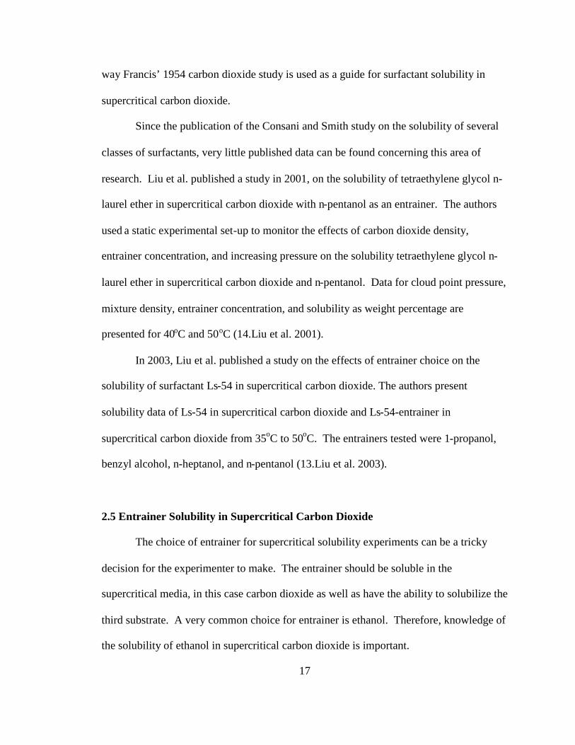
When dealing with a ternary LLV system, a three phase isothermal flash is carried out.

Figure 6 shows the algorithm for a ternary LLV system isothermal flash:

Figure 6. Algorithm for LLV Isothermal Flash Calculations (25.Seader & Henley1998).

Search for three-phase solution

Search for 21 , LL solution

Search for1, LV solution

Single-phasesolution

StartF, z fixed

P, T of equilibriumphases fixed

Solution found with

10 10

Solution found with

10 1

Solution found with

10 10 or

> 1

Vapor

> 1liquid

Solution notfound

Solution notfound

Solution notfound

32

3.4 Activity Coefficient Models

The activity coefficient models mentioned in section 3.3 deserve a more detailed

explanation. This section will present some details for each activity coefficient model.

Activity coefficients can be determined experimentally by measuring various properties:

vapor pressure lowering, freezing point depression, boiling point elevation, and osmotic

pressure (31.Walas 1985).

The van Laar model for activity coefficients uses a reciprocal form of the excess

Gibbs energy as a basis for activity coefficient determination:

21

11BxAxG

RTex 50

The activity coefficients are then given by:

2

21

21ln

BxAx

BxA 51

2

21

12ln

BxAx

AxB 52

where A is given by Equation 53:

2

11

2211 ln

ln1lnln

xx

A 53

and B is given by Equation 54:

2

22

1122 ln

ln1lnln

xx

B 54

A couple important points should be noted regarding the van Laar activity

coefficient model assumptions: mixtures consist of molecules of the same size and shape

33

and the van der Waals equation of state can accurately describe the mixture behavior

(23.Sandler 1999). The van Laar model is now viewed as an empirical model for activity

coefficients due to poor representation with van der Waals parameters (31.Walas 1985).

The Regular Solutions Theory comes from Scatchard and Hildebrand who

determined some very important properties of mixtures: excess volume is nearly zero,

excess entropy is nearly zero, and very few mixtures were actually well represented by

the van der Waals equation of state. Scatchard proposed using the experimental change

in the internal energy on vaporization versus an equation of state to calculate the internal

energy change in vaporization (23.Sandler 1999). The Regular Solution Theory

represents the change in the internal energy on vaporization as a ratio to volume. This

ratio of the change in the internal energy on vaporization to volume is called the

solubility parameter, δ. Activity coefficients from the Regular Solutions Theory take the

following form:

221

22

11ln

RTV L

55

and

221

21

22ln

RTV L

56

In Equations 55 and 56 LV1 and LV2 are the liquid molar volumes of component 1 and

component 2.

34

The terms 1and 2are the volume fractions of the mixture are defined by Equations 57

and 58:

LL

L

VxVxVx

2211

111 57

and

LL

L

VxVxVx

2211

222 58

Perhaps the most attractive feature of the Regular Solution Theory is that activity

coefficients can be ascertained based solely on knowledge of the pure liquid molar

volumes. However, the Regular Solution Theory is not good to use when dealing with

mixtures of polar liquids because of the aforementioned assumptions (31.Walas 1985).

The Wilson equation takes into account the interactions between molecules. This

interaction is characterized in terms of probabilities, i.e. the probability of finding a

certain molecule within a local vicinity of another molecule. The Wilson equation for

activity coefficients involves a two parameter equation for the excess Gibbs energy of a

mixture. The excess Gibbs energy using the Wilson equation is given by:

2121221211 lnln xxxxxxRTG ex

59

The activity coefficients using the Wilson equation for Gibbs excess energy is given by:

2121

221

2121

21221211 lnln

xxx

xxx

xx

60

2121

121

2121

11221212 lnln

xxx

xxx

xx

61

35

The two parameters, Λ12 and Λ21 can be determined if infinite dilution activity

coefficients for both components are known as shown in Equations 62 and 63:

21121 1lnln 62

12212 1lnln 63

The Wilson equation for activity coefficients models mixtures of polar and non-

polar substances very well. The Wilson equation can also be used to model multi-

component mixtures using only binary parameters. Unfortunately, the Wilson equation

also has certain challenges: neither parameter can be negative if the entire composition

range is to be characterized, liquid-liquid immiscibility cannot be described, and multiple

roots can exist for an activity coefficient whose value is below one (31.Walas 1985).

The NRTL (Non-Random Two Liquid) equation for activity coefficients

developed by Renon and Prausnitz involves three parameters (α, τ12 , τ21). NRTL is based

on a two-cell theory. The two-cell theory describes a liquid mixture as cells of molecules

of liquid one and liquid two enveloped by other cells of the same molecules (31.Walas

1985). The Gibbs energy of the two cells is given as:

2121111

1 gxgxg 64

and

22221212

2 gxgxg 65

It should be noted that g11 and g22 are the pure component Gibbs energies and that g12 is

take to be equal to g21 . The excess Gibbs energy of the cells is then described by

Equation 66:

22121221121211 ggxxggxxg ex 66

36

In Equation x12 and x21 are the local mole fractions and are defined as follows:

RTgx

RTgxxx

/exp/exp

11121

21122

11

21

67

RTgx

RTgxxx

/exp/exp

22121

12121

22

12

68

Theα12 term in Equations 67 and 68 is a characteristic constant representing the non-

randomness of the mixture. It should be noted thatα12 values ranging from 0.1 to 0.5 do

not have that great of an affect on the activity coefficient. Figure 7 shows how the value

ofα12 changes the activity coefficient of a particular species. According to Renon and

Prausnitz, using values ranging from 0.2 to 0.47 forα12 should give satisfactory results

(31.Walas 1985).

Figure 7. NRTL Activity Coefficient Dependence onα12 Value (31.Walas 1985).

37

The local mole fractions x21 and x12 can be found by solving the following equations:

RTggxx

RTggxx

//exp

11211221

112112221

69

RTggxx

RTggxx

//exp

22121212

221212112

70

Putting Equations 69 and 70 into Equation 66 the excess Gibbs energy for the system

becomes Equation 71:

2112

1212

2121

212121 xxG

GGxx

Gxx

RTG ex 71

Equation 59 is a slightly simplified form. The terms τ21, τ12, G21, and G22 must be

defined.

The terms τ21 and τ12 take the following form:

RTgg /111221 72

RTgg /221212 73

The terms G21 and G22 take the following form:

211221 exp G 74

121212 exp G 75

38

The activity coefficients based on the NRTL equation take the form of Equations 76 and

77:

22121

1212

2

2121

2121

221ln

GxxG

GxxG

x

76

and

22121

2121

2

1212

1212

212ln

Gxx

GGxx

Gx

77

The NRTL equation for activity coefficients offers excellent modeling capabilities

concerning liquid-liquid equilibrium. NRTL can be extended to multi-component

mixtures using only data for binary pairs without much difficulty. Perhaps the biggest

setback with the NRTL equation is the necessity of three parameters. Having three

parameters allows for NRTL to model experimental data with greater accuracy then van

Laar and Wilson (31.Walas 1985).

The UNIQUAC (Universal Quasi-Chemical) equation for activity coefficients

developed by Abrams and Prausnitz is a model based upon statistical mechanics and

association of groups. UNIQUAC calculates the excess Gibbs energy of a mixture as a

function of the differences in molecule size as well as the energy differences between the

molecules. Equation shows how the excess Gibbs energy for a mixture is calculated:

RTresidualG

RTialcombinatorG

RTG exexex

78

The combinatorial portion of Equation 66 represents the difference in the shapes and

sizes of the molecules. The residual portion of Equation 78 represents the energy

difference between the molecules (23.Sandler 1999).

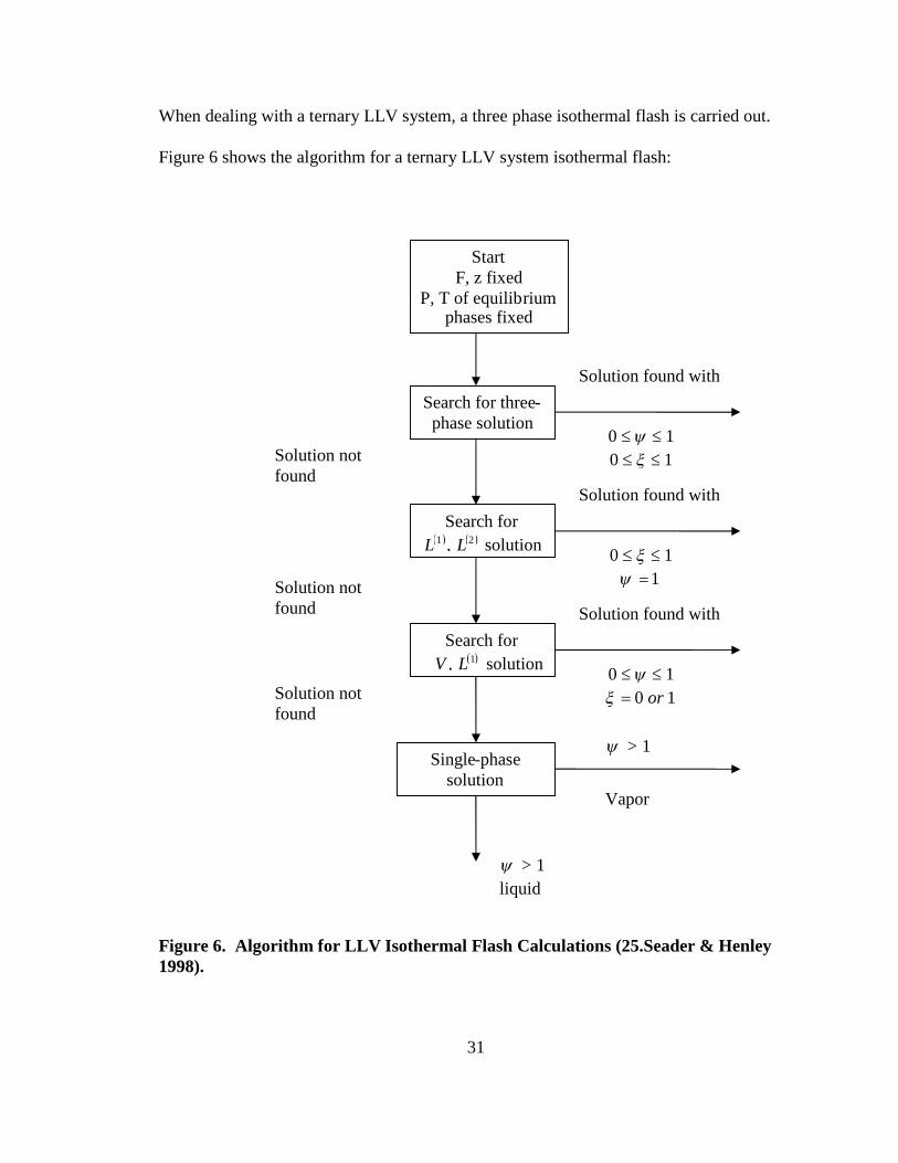
39

The combinatorial part of Equation 78 is calculated by using the following

equation:

i

i

iii

i

i

ii

ex

qxz

xx

RTialcombinatorG

ln

2ln 79

Equation 79 has several parts that must also be defined. The term represents the

segment fraction of species i and is defined by the following equation:

jj

iii rx

rx 80

In Equation 79, z represents the average coordination number, which is usually taken as

ten. The θ term in Equation 79 represents the area fraction of species i and is defined as:

jj

iii qx

qx 81

The q term in Equation 79 represents the surface factor of a particular segment of the

molecules being studied. The r term in Equation 80 represents the volume factor of a

particular segment of the molecules being studied. The q and r terms are determined

through crystallography experiments (31.Walas 1985).

The residual component in Equation 78 is determined by the following equation:

jijii

ex

xqRTresidualG

ln 82

The term τji takes the energy differences between the molecule segments into account and

is defined as:

RT

uu jjijji

ln 83

40

In Equation 83, uij is the average interaction energy between two particular segments of

the molecules.

The UNIQUAC equation can be utilized to describe multi-component mixtures

using only binary parameters. Liquid-liquid phase equilibrium can be described

sufficiently using UNIQUAC. Mixtures of vastly different molecular sizes can be

characterized with UNIQUAC without too much difficulty. Challenges for the

UNIQUAC equation include occasional poor representation of a mixture and the

mathematical intricacy of the equations (31.Walas 1985).

Along the same line as the UNIQUAC equation, the UNIFAC (UNIQUAC

Functional Group Activity Coefficients) equation, developed by Fredenslund, Jones, and

Prausnitz also relies on statistical mechanics and association of groups. The UNIFAC

equation involves the sum of a combinatorial and residual component to calculate the

activity coefficient of each component shown in Equation 85:

Ri

Cii lnlnln 84

The combinatorial component of Equation 84 is defined as:

i

jji

ii

i

ii

i

iCi lx

xlq

zx

ln2

lnln 85

The only new aspect of Equation 73 as compared to the UNIQUAC equation is the l

term. Every other component of the combinatorial part of the UNIFAC equation is the

same as in the UNIQUAC equation. The l term in Equation 85 is a function involving the

surface area and volume parameters of the molecule segment.

41

The l term in Equation 85 is defined as:

12

iiii rz

qrl 86

The residual component of Equation 72 is defined as:

k

ikk

ik

Ri v lnlnln 87

The term Γk represents the residual group activity coefficient, while the term Γk(i)

represents the residual activity coefficient of group k in a solution that only has molecules

of component i.

TheΓk term is defined by the following equation:

mn

nmn

kmm

mmkmkk q

ln1ln 88

TheΓk(i) term is also defined by Equation 88, just involving the groups of each individual

molecule. The ψ terms represent the interaction energies of the various segments of the

molecules. The ψ term is defined as:

Ta

RTUU mnnnmn

mn expexp 89

The interaction energies between the various molecule segments can be looked up in

charts (7.Fredenslund & Jones & Prausnitz 1975).

3.5 The Model

The model used to describe these systems was the Peng-Robinson-Stryjek-Vera

(PRSV) equation of state with Wong-Sandler (WS) mixing rules. The improved Peng-

Robinson equation of state proposed by Stryjek and Vera abbreviated PRSV (27.Stryjek

42

& Vera 1986), offers a couple of minor adjustments that allow for more accurate vapor-

liquid equilibrium calculations.

The Peng-Robinson (PR) equation of state (18.Peng & Robinson 1976) has been

one of the models of choice used to describe chemical system behavior. The PR equation

of state is a slight adjustment to the attractive and repulsive forces represented by van der

Waals’ hard sphere equation. The PR equation of state takes the following form:

)()()(

)( bvbbvvTa

bvRT

P

90

The PRSV equation of state takes the form:

)()()( bvbbvva

bvRTP

91

Equations 90 and 91 are often expressed in terms of the compressibility factor Z, which

takes the form:

RTPvZ 92

So, Equation 91 represented in terms of equation 92 takes a cubic form:

0)()23()1( 32223 BBABZBBAZBZ 93

Where A and B are represented as follows:

22

2

TRaPA 94

RTbP

B 95

Equation 93 generates up to three roots for Z depending on the number of phases present

in the system. The lowest positive value of Z in the two-phase region represents the

43

molar volume of the liquid. The highest positive value of Z in the two-phase region

represents the molar volume of the vapor. The repulsive force correction b, is

represented by:

c

c

PRT

b077796.0

96

The repulsive force correction, b, takes into account the forces between molecules when

they collide with each other. The frequency and force of these molecular collisions

directly affects the overall pressure of a system. Additionally, as a result of the frequent

collisions between molecules, the true volume occupied by the molecules would be

smaller. The true volume would also be smaller if the engineer made the assumption that

the molecules are perfect spheres.

Meanwhile, attractive forces between molecules lower the force and frequency of

the molecular collisions. The attractive forces between the molecules must also be taken

into account for model accuracy.

The attractive force correction a, is represented by:

c

c

PTR

a22457235.0

97

The term is represented by:

)]1(1[ )21()2

1(rT 98

here is only a function of the acentric factor, . The improvement suggested by Stryjek

and Vera occurs with . Here Stryjek and Vera represent as:

)7.0)(1( 5.010 rr TT 99

44

The term 0 is represented as a function of the acentric factor:

320 0196554.017131848.04897153.1378893.0 100

The acentric factor is essentially a measure of how the forces around a molecule cause it

to depart from spherical symmetry. Tr, the reduced temperature, with T and Tc in Kelvin

takes the form:

cr T

TT 101

The term 1 is unique to every compound.

Wong-Sandler mixing rules (32.Wong & Sandler 1992) are employed to improve

the accuracy of modeling binary system behavior. The mixing rules are based on the

setting the excess Helmholtz free energy at infinite pressure to an activity coefficient

model using the following approximation:

iE

iE

iE

iE xTaxPhighTaxbarPTaxbarPTg ,,,,1,,1, 102

The Wong-Sandler (WS) mixing rules take the following form:

ijjimm RTabxxRTab )()( 103

)1(2

)()()( ij

jjiiij k

RTabRTabRTab

104

where kij is an interaction parameter.

45

It should be noted that Equation 103 only gives one value for the left hand side of the

equation. In order to determine bm and am of Equation 103 the following equations are

used:

i i

ii

E

i ijjji

m

RTbax

CRTa

RTabxx

b1

105

C

xaba

xba iE

i i

iimm

106

where

62322.02

12ln

C for PRSV equation of state. The excess Gibbs energy

is given by the following equation:

iiex xRTG ln 107

Since the excess Helmholtz energy is equal to the excess Gibbs energy, plugging the

answer from Equation 107 into Equations 105 and 106 is sufficient for modeling

purposes. The fugacity coefficient of the component i in the mixture, i, is determined

by the following equation:

)414.0ln()414.2ln(

2

828.2)ln()1()ln(

BZBZ

BB

A

Ax

BABZZ

BB ij

ijii

i 108

The fugacity coefficient is then used to calculate solubility in the supercritical fluid in the

following equation:

PfactorPoyntingTPx

yi

satii

i )exp()(

109

46

Psat(T) is the vapor pressure of the compound of interest at the experimental temperature.

The Wagner equation for ethanol vapor pressure (19.Poling & Prausnitz & O’Connell

2001) takes the following form:

55.25.1 588.18762.417831.168587.8ln

TT

P cr 110

The term τis defined by the following equation:

cTT

111

The Poynting factor in Equation 109 is represented as

RTVPP

factorPoynting msat )(

112

The molar volume, Vm, is found by using the Rackett Equation (22.Rackett 1970):

c

Tcc

m PZRT

Vr ])1(1[ )7

2(

113

Zc is the critical compressibility factor and is represented by:

c

ccc RT

VPZ 114

The liquid phase molar compositions are represented by x1 , x2, and x3. Carbon dioxide is

x1. Ethanol is x2. The surfactant is x3. The liquid phase molar composition thus takes

the shape:

1321 xxx 115

47

The vapor phase molar compositions are represented by y1, y2, and y3 where carbon

dioxide is y1 , ethanol is y2, and the surfactant is y3. The vapor phase molar composition

takes the form:

1321 yyy 116

It should be noted that a cubic equation of state does not generate every

thermodynamic property of a compound or mixture accurately. In particular, the liquid

molar volumes that the PRSV equation of state calculates can be a significant source of

error in analysis. Stryjek and Vera report liquid molar volume errors no higher than 8%

for paraffins of low molecular weight. Errors associated with butane through heptane

stay in a small range 6%. Higher hydrocarbons have larger and negative errors for

liquid molar volumes. The molar volume error associated with polar compounds can be

high as well. For example, methanol has an average deviation of –20% between the

actual liquid molar volume and the PRSV calculated liquid molar volume. Deviations

ranging from –2% to –4% are common for alcohols of higher molecular weight than

methanol (27.Stryjek & Vera 1986).

Because the error associated with the liquid molar volumes predicted by the

PRSV equation of state can be very high, the PRSV equation of state is not used to

determine the amount of liquid carbon dioxide used in each experimental run. Instead the

Improved Rackett Equation (26.Spencer & Danner 1972) is used.

The Improved Rackett Equation takes the form:

c

Trac

m PZRT

Vr ])1(1[ )7

2(

117

48

Zra is a constant that is determined experimentally for each compound. For carbon

dioxide Zra is reported as 0.2736. The average percent deviation in liquid molar volumes

using the Improved Rackett equation is 0.72% (26.Spencer & Danner 1972).

3.6 Critical Property Estimation

Often times when engineers look to modeling observed phase behavior an

equation of state involving pure component data is utilized. Some cubic equations of

state use pure component critical properties (Pc, Tc, Vc, Zc, and ω) to describe the

consequent phase behavior of mixtures. Frequently though, the critical properties for one

component are not available.

Fortunately, methods exist that allow for a reasonably good estimation of pure

component critical properties. One such method for critical property estimation that has

been employed successfully is the Joback group contribution method (28.Tester &

Modell 1997). The Joback method breaks down molecules into certain functional groups.

A particular value for each functional group is then assigned with respect to critical

pressure, critical temperature, critical volume, and the normal boiling temperature. The

Joback group contribution method for critical property estimation was originally tested

on over 400 compounds. Joback also developed a group contribution method to

determine: enthalpy of formation, Gibbs free energy of formation, and the ideal gas state

heat capacity (28.Tester & Modell 1997).

49

To estimate the critical temperature on absolute scale, Joback proposes the

following equation:

2

965.584.j j

jTi

jTi

j

bc

ccvv

TT 118

The critical pressure in units of bar is found by Equation 119:

2

0032.113.0

1

j

Pi

ja

c

cjvn

P 119

where na is the actual number of atoms in the molecule.

The critical volume in units of cm3/mol is given as:

j

Vijc cj

vV 5.17 120

The term ijv in Equations 118-120 represents the number of groups of the type j in

compound i. The summation term in Equations 118-120 includes all the groups found in

compound i. The terms ,,cc PT and

cjV can be found in charts provided by Joback

(28.Tester & Modell 1997).

One more property crucial to developing an accurate mathematical model is the

acentric factor. The acentric factor of a compound can be estimated by using the

compound boiling point and the calculated values for critical temperature and critical

pressure. The acentric factor is calculated by the following equation:

1013.1

log17

310

c

c

b

c

bP

TTT

T

121

50

In Equation 121 the units for Tb and Tc are Kelvin while the units for Pc are bar (28.Tester

& Modell 1997).

3.7 Phase Behavior Classification

An accurate analytical model can eliminate the need for excessive experimental runs.

Ideally, the analytical model is developed to describe phase behavior, then carefully

planned and executed experiments can be used to adjust the model parameters. The

analytical model can be used to determine what type of classification the system of

interest falls into.

Binary mixtures fall into six categories: type I, type II, type III, type IV, type V

and type VI. Type I phase behavior is usually exhibited by components with similar

critical properties or chemical structures. The critical mixture curve of a type-I binary

system moves from the critical point of the heavier component to the critical point of the

lighter component. Type II phase behavior has three phase equilibrium (LLV). The

three phase equilibrium ends with a UCEP when the temperature is below either

component’s critical temperature. Between the critical points of the two components, the

phase behavior is similar to that of type-I mixtures. A miscibility gap exists for type-II

binary systems at low temperatures (15.McHugh & Krukonis 1986).

Type III phase behavior is displayed by mixtures with critical properties that are

significantly different. In type-III phase behavior, a three phase equilibrium (LLV)

occurs near the more volatile component critical point. The LLV equilibrium for type-III

systems is analogous to that of type-II systems below the LCST. Type-I phase behavior

can be seen at temperatures far below the critical temperature of the more volatile

51

component. Two branches of the critical mixture curve exist for a type-III binary system.

One part of the critical mixture curve starts at the critical point of the more volatile

component, crosses the LLV line, and ends with the LCST. The other part of the critical

mixture curve starts at the less volatile critical point and ends with a UCEP (15.McHugh

& Krukonis 1986).

Type-IV behavior is seen in systems where the critical mixture curve has two

branches. However, compared to type-III behavior, the critical mixture curve at the more

volatile component does not cross the LLV line. The critical mixture branch for the more

volatile component ends with a UCEP. For the less volatile component, the critical

mixture curve begins at the lower volatile component’s critical point and ends with a

LCEP. A type-IV mixture above its critical pressure can divide into two phases with a

pressure increase (15.McHugh & Krukonis 1986). Type-V phase behavior is similar to

that of type-III except liquid-liquid immiscibility below the LCST does not exist (15

McHugh & Krukonis 1986). Type-VI phase behavior is seen when two critical mixture

curves exist. One critical mixture curve runs between the critical points of both

components. The second critical mixture curve runs between the LCEP and the UCEP

(17.Ozdemir 1994). Figure 8 shows all of the phase behavior classifications

52

Figure 8. Phase Behavior Classifications (17.Ozdemir 1994)

Ternary mixture phase behavior is categorized into three groups: type I, type II,

and type III. The groups are distinguished by the LLV regions that exist for the mixture.

Type I phase behavior is exhibited by ternary systems that do not have an immiscibility

region for LLV equilibrium. Type II phase behavior is exhibited by ternary systems that

have a miscibility gap in the liquid phase. Type III phase behavior is exhibited by ternary

systems where the miscibility gap of the LLV equilibrium touches a binary axis of a

pressure-composition diagram (15.McHugh & Krukonis 1986).

53

Chapter 4

Experimental

The experimental set-up for determining the solubility of Triton X-114 and

Tergitol 15-S-9 in supercritical carbon dioxide has been described briefly in the theory

chapter, but will be described in more detail here. The equipment purchased and used

will be discussed as well as the procedure and materials used for the experiments.

4.1 Equipment

In order to determine surfactant solubility in supercritical carbon dioxide a

SPM20 Super Phase Monitor, shown in Figure 9, was purchased new from Thar

Technologies in Pittsburgh, Pennsylvania.

54

Figure 9. SPM20 Super Phase Monitor (30.Thar Technologies 2004)

The Super Phase Monitor contains two sapphire windows, one for a camera and one for a

light source. The solubility cell shown in Figure 7 is made out of 316 stainless steel and

can be adjusted from a minimum of 5 ml to a maximum of 15 ml.

55

Figure 10. The Solubility Cell (30.Thar Technologies 2004)

Solubility experiments can be done under one of two settings with the SPM20 Super

Phase Monitor. Figure 11 and Figure 12 show both set-ups, one being a fixed frit setting

and the other being a movable frit setting. The fixed frit setting allows for experiments to

be done at a constant volume. The movable frit setting allows for experiments to be done

with an adjustable volume. The experiments conducted in this study were done with the

movable frit setting.

56

Figure 11. Fixed Frit Setting (30.Thar Technologies 2004)

57

Figure 12. Movable Frit Setting (30.Thar Technologies 2004)

The operating pressure and temperature limits monitored by the controller, shown

in Figure 13 are 413 bar and 150oC, with an error of 0.1 bar and 0.1oC, respectively.

58

Figure 13. SPM20 Super Phase Monitor Controller (30.Thar Technologies 2004)

59

Preceding the SPM20 Super Phase Analyzer is an Isco 100DX Syringe Pump (100 ml

volume) shown in Figure 14.

Figure 14. Isco 100DX Syringe Pump (8.Isco 1999)

Figure 15 shows a Lauda Econoline Low-Temperature Thermostat RE120 that circulates

antifreeze cools the Isco 100DX Syringe Pump.

CO2

60

Figure 15. Lauda Econoline Low-Temperature Thermostat RE-120 (11.Lauda 1999)

Figure 16 shows how the circulating antifreeze cools the carbon dioxide.

61

Figure 16. Isco 100DX Syringe Pump Cooling Jacket Set-Up (8.Isco 1999)

A Ruska manual pump is connected to the SPM20 Super Phase Analyzer to provide

pressure during experimental runs. The Ruska manual pump is charged with deionized

water and has an operating pressure limit of 10,000 psi (689 bar). The Isco Syringe

Pump, the Low-Temperature Thermostat, and the Ruska manual pump were all

previously purchased for earlier projects.

62

4.2 Experimental Set-Up

Figure 17. Experimental Set-Up

Figure 17 shows the experimental set-up used for this research in its entirety. The

static experimental set-up was chosen for a few reasons. Solubility data can be quickly

and easily obtained at several temperatures with one experimental run. Pressure inside

the solubility cell can be adjusted quickly and easily with a variable volume cell. Any

phase changes can be determined visually, so passing a sample of the mixture through a

UV/Vis or IR detector is not necessary.

63

Furthermore, inaccurate solubility measurements may be observed using the

dynamic experimental set-up because the surfactants of interest for this research are both

liquids at room temperature. The supercritical fluid-entrainer mixture may actually push

the surfactant out of the solubility cell without solubilizing it. Clogging in the piping can

also occur with the dynamic experimental set-up.

4.3 Procedure and Materials

Carbon dioxide is pumped into an Isco 100DX Syringe Pump. A Lauda

Econoline Low-Temperature Thermostat RE120 cools syringe pump to –3oC by

circulating antifreeze. The cooling of the syringe pump is done to ensure that the carbon

dioxide is in the liquid phase when it is pumped into the solubility cell. The surfactant,

Triton X-114 or Tergitol 15-S-9 (Aldrich) is weighed in a beaker then transferred to the

open solubility cell. The beaker is reweighed and recorded. HPLC grade ethanol

(Aldrich), the entrainer, is weighed in a separate beaker and transferred to the solubility

cell. The ethanol beaker is reweighed and recorded.

The solubility cell is then brought to a minimum volume using a Ruska manual

pump while still open. Adjusting the solubility cell to a minimum volume is done so that

the presence of air can be considered negligible. The solubility cell is then sealed with

the magnetic stirrer. Low-pressure carbon dioxide is pumped into the solubility cell

while the outlet valve is open to vacate the solubility cell of air completely. The outlet

valve is closed and liquid carbon dioxide is pumped into the solubility cell. Once liquid

carbon dioxide is visible on the television, the solubility cell volume is slowly expanded

64

to its maximum volume. Liquid carbon dioxide flow into the solubility cell is shut off

when the pressure inside the solubility cell increases one to two bars per second.

The pressure inside the solubility cell is allowed to reach equilibrium. After five

to ten minutes, the initial pressure and temperature are recorded. The solubility cell is

then shifted to a horizontal position such that the liquid-liquid interface is visible in the

camera view cell. The magnetic stirrer is turned on to achieve homogeneity and the

solubility cell is heated to temperature (35oC, 40oC, 45oC, 50oC) with the controller and

heating element. Once the mixture reaches the experiment temperatures listed above the

magnetic stirrer is turned off. A Ruska manual pump then pressurizes the solubility cell

by forcing an incompressible fluid (deionized water) to move the piston inside the

variable volume solubility cell. Pressurization continues until a cloud is observed in the

view cell and the mixture becomes clear again with no discernable liquid-liquid interface.

This procedure is continued until five cloud point pressures have been recorded at the

experiment temperature. The average of these pressures is reported here with its standard

deviation. When the mixture is heated from one experimental temperature to the next

experimental temperature the magnetic stirrer is turned on.

4.4 Clean-Up

In between each experiment to determine surfactant solubility in supercritical

carbon dioxide, the solubility cell undergoes a detailed cleaning process. The cleaning

process is necessary to ensure that no contamination occurs in subsequent runs. After

sufficient data points have been collected at experimental temperatures the heating

element is turned off and the cell is returned to a vertical position. The outlet valve of the

65

solubility cell is opened such that depressurization occurs at approximately two to three

bars per minute. The slow depressurization rate is necessary to prevent clogging in the

outlet valve and line.

Once pressure inside the solubility cell is completely released, the magnetic stirrer

is unsealed from the top of the machine. The solubility cell is then inverted 180o to

remove the rest of the ethanol-surfactant mixture. The camera, inlet and outlet valves,

thermocouple, and light are unplugged from the solubility cell. The solubility cell is then

unscrewed from the base of the Supercritical Phase Analyzer. The two o-rings on the

bottom of the solubility cell are removed and rinsed thoroughly with deionized water

followed by denatured ethanol (Fischer). The o-rings are then allowed to air-dry.

The frit on the movable piston is unscrewed next. The frit is washed thoroughly

with deionized water followed by denatured ethanol. The frit is then allowed to air-dry.

The piston is rinsed with deionized water followed by denatured ethanol, wiped dry. The

piston is then allowed to air-dry.

The stirrer is removed from the magnetic stirrer and rinsed thoroughly with

deionized water followed by denatured ethanol. The stirrer is then allowed to air-dry.

The solubility cell cap that houses the stirrer is rinsed thoroughly with deionized water

followed by denatured ethanol. The solubility cell cap is then allowed to air-dry.

The solubility cell is rinsed thoroughly with deionized water followed by

denatured ethanol. The solubility cell is then allowed to air-dry. Air-drying times for all

components were a minimum of ten minutes.

After air-drying is complete, the solubility cell components are reassembled. A

second cleaning is done at this point with pure carbon dioxide. Liquid carbon dioxide is

66

pumped into the solubility cell, which is at its maximum volume. The flow of liquid

carbon dioxide is shut off once the solubility cell is full as evident from pressure

increases of one to two bars per second noted on the controller. The magnetic stirrer is

turned on to improve cleaning efficiency. This solubility cell cleaning process with

liquid carbon dioxide continues for ten minutes, then the solubility cell is depressurized

two to three bars per minute.

After the pure carbon dioxide cleaning process, the magnetic stirrer and the

solubility cell are removed from the Supercritical Phase Monitor and once again allowed

to air-dry.

67

Chapter 5

Results and Discussion

This section will used to present the experimental results. A discussion about the

accuracy of the improved Rackett equation for liquid molar volumes compared to values

obtained by the PRSV equation of state will be presented. Results will be presented for

binary and tertiary systems. A discussion about the factors that can influence component

solubility in supercritical carbon dioxide will also be given.

5.1 A Comparison of the Improved Rackett Equation to the PRSV Equation

Further discussion about the accuracy of the Improved Rackett Equation molar

volumes compared to the PRSV equation of state molar volumes is warranted. As

previously mentioned in chapter two the error associated with molar volume calculations

using the PRSV equation of state can be very high – greater than 20% (18.Stryjek & Vera

1986). In comparison, the average relative deviation of the Improved Rackett Equation is

less than 1% (17.Spencer & Danner 1972).

The Improved Rackett Equation was used in the data analysis of these

experiments due to noted difference in error versus the PRSV equation of state. For

carbon dioxide from 0oC to 31oC, the error associated with the Improved Rackett

Equation molar volumes to experimental carbon dioxide molar volumes ranged from

0.07% to –5.4% difference. For the same pressure and temperature range mentioned

68

above the error associated with the PRSV equation of state molar volumes ranged from

26.9% to –28.6% compared to experimental carbon dioxide molar volumes.

Figure 18 shows how the Improved Rackett Equation and the PRSV equation of

state compare to experimental carbon dioxide molar volume measurements (1.Angus &

Armstrong& de Reuck 1976).

Molar Volume Comparison for Carbon Dioxide

0

20

40

60

80

100

120

140

0 2 4 6 8 10 12 14 16 18 20 22 24 26 28 30Temperature (Celsius)

Mol

arV

olum

e(c

m3/

mol

)

CO2 Tables IRE PRSV

Figure 18. Molar Volume Comparison

As Figure 18 shows, molar volume values tabulated by the Improved Rackett Equation

are almost the same as the experimental measurements taken for carbon dioxide up to the

critical temperature. The molar volume values tabulated from the PRSV equation of state

are very inaccurate relative to the values provided by the Improved Rackett Equation.

Above room temperature the PRSV molar volume values become significantly

inaccurate.

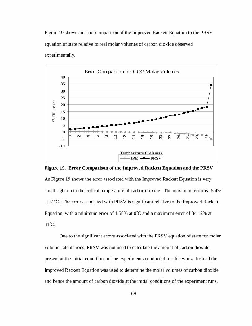
69

Figure 19 shows an error comparison of the Improved Rackett Equation to the PRSV

equation of state relative to real molar volumes of carbon dioxide observed

experimentally.

Error Comparison for CO2 Molar Volumes

-10

-5

0

5

10

15

20

25

30

35

40

0 2 4 6 8 10 12 14 16 18 20 22 24 26 28 30

Temperature (Celsius)

%D

iffe

renc

e

IRE PRSV

Figure 19. Error Comparison of the Improved Rackett Equation and the PRSV

As Figure 19 shows the error associated with the Improved Rackett Equation is very

small right up to the critical temperature of carbon dioxide. The maximum error is -5.4%

at 31oC. The error associated with PRSV is significant relative to the Improved Rackett

Equation, with a minimum error of 1.58% at 0oC and a maximum error of 34.12% at

31oC.

Due to the significant errors associated with the PRSV equation of state for molar

volume calculations, PRSV was not used to calculate the amount of carbon dioxide

present at the initial conditions of the experiments conducted for this work. Instead the

Improved Rackett Equation was used to determine the molar volumes of carbon dioxide

and hence the amount of carbon dioxide at the initial conditions of the experiment runs.

70

5.2 Critical Property Estimation of Surfactants

In order to develop mathematical models to represent the phase behavior of the

binary and ternary systems of interest for this research, the critical properties (pressure,

temperature, and volume) for the surfactants had to be estimated. The Joback Method

was used to estimate the critical properties of Triton X-114 and Tergitol 15-S-9. Table 1

shows the critical properties of Triton X-114 and Tergitol 15-S-9 according to the Joback

method and the acentric factors:

Table 1. Critical Properties of SurfactantsChemical Tc (Kelvin) Pc (bar) Vc (cm3mol-1) ω

Triton X-114 613.81 6.8998 1759.5 0.2012

Tergitol 15-S-9 734.87 5.5233 1952.5 -0.2200

Sample calculations for determining the critical properties as well as the acentric factors

of the surfactants can be found in Appendix C.

5.3 Carbon Dioxide and Surfactant Binary Systems

Experiments were conducted with carbon dioxide and both surfactants, Triton X-

114 and Tergitol 15-S-9 as binary systems. At all temperatures, 35oC to 50oC, the

surfactant Triton X-114 is insoluble in supercritical carbon dioxide up to 320 bar.

Similar results were obtained with the carbon dioxide – Tergitol 15-S-9 binary system.

Tergitol 15-S-9 is insoluble in supercritical carbon dioxide up to 320 bar at all

temperatures from 35oC to 50oC. Pressurization beyond 320 bar for both systems was not

71

achieved because the variable volume cell had already reached the five-milliliter

minimum volume.

5.4 Carbon Dioxide – Ethanol – Triton X-114 Ternary System

The addition of ethanol as an entrainer to the carbon dioxide-Triton X-114

mixture allows for Triton X-114 to become soluble in supercritical carbon dioxide.

Various compositions were examined for the ternary mixture. Table 2 displays the

mixture compositions studied for this work.

Table 2. Ternary Mixture Compositions Studied with Triton X-114Mixture x1 x2 x3

1 0.9769 0.0229 0.00022 0.9321 0.0675 0.00043 0.9466 0.0530 0.0005

Carbon dioxide is represented by x1. Ethanol is represented by x2. Triton X-114 is

represented by x3. Observed cloud point pressures for the carbon dioxide-ethanol-Triton

X-114 ternary mixtures range from 95.6 bar at 35oC to 143.8 bar at 50oC. Table 3 shows

the cloud pressures reported in bars, observed for each mixture at each temperature.

Table 3. Observed Cloud Point Pressures of Triton X-114 MixturesMixture Cloud Point Pressure (bar)

@ 35oC @ 40oC @ 45oC @ 50oC1 99.9 114.7 128.6 143.12 n/a n/a 129.1 143.83 95.6 107.4 122.2 134.3

Cloud point pressures are not reported for mixture two at 35oC and 40oC because one

phase had already been achieved before the experiment temperature had been attained.

Figure 16 shows a P-x diagram for Triton X-114 in the carbon dioxide-ethanol mixture.

72

P-x Diagram Triton X-114 Solubilized in CO2 + Ethanol

80

90

100

110

120

130

140

150

0.00015 0.00025 0.00035 0.00045 0.00055Mole Fraction Triton X-114

Clo

udP

oint

Pre

ssur

e(b

ar)

35 C 40 C 45 C 50 C

Figure 20. P-x Diagram of Triton X-114 in Carbon Dioxide-Ethanol

As Figure 20 and Table 3 indicate, the cloud point pressure of the ternary mixture

increases as the temperature of the mixture increases.

As mentioned in chapter four, five measurements for cloud point pressure were

taken for each temperature. This was done to ensure accuracy and precision in

observations. One measure of precision is standard deviation. A lower standard

deviation of measurements means precision has been achieved. The highest standard

deviation in cloud point pressure measurements at any temperature for this study is

0.2588 bar. Table 4 shows the standard deviations of the cloud point pressure

measurements in bars for each mixture at each temperature.

Table 4. Standard Deviations of Cloud Point Pressure MeasurementsMixture Standard Deviation (bar)

@ 35oC @ 40oC @ 45oC @ 50oC1 0.2588 0.1225 0.1095 0.18712 n/a n/a 0.2345 0.14143 0.1226 0.2074 0.0707 0.1817

73

5.5 Carbon Dioxide – Ethanol – Tergitol 15-S-9 System

The addition of ethanol as an entrainer to the carbon dioxide-Tergitol15-S-9

mixture allows for Tergitol 15-S-9 to become soluble in supercritical carbon dioxide.

Various compositions of the ternary mixture were studied. Table 5 shows the

compositions of ternary mixtures examined in this study.

Table 5. Ternary Mixture Compositions Studied with Tergitol 15-S-9Mixture x1 x2 x3

1 0.9441 0.0557 0.00022 0.9231 0.0766 0.0003

In this case carbon dioxide is represented by x1. Ethanol is represented by x2. Tergitol

15-S-9 is represented by x3. Observed cloud points for these mixtures range from 89.58

bar to 154.36 bar. Table 6 displays the observed cloud point pressures in bar of the

ternary mixtures

Table 6. Observed Cloud Point Pressures of Tergitol 15-S-9 MixturesMixture Cloud Point Pressure (bar)

@ 35oC @ 40oC @ 45oC @ 50oC1 125.3 154.4 127.3 116.02 89.6 120 n/a n/a

Cloud point pressures are not reported for mixture two because one phase had already

been achieved before the experiment temperature could be attained. Figure shows a P-x

diagram for the carbon dioxide-ethanol-Tergitol 15-S-9 system.

74

Cloud Point Pressure vs. Mol Fraction Tergitol 15-S-9 Solubilized

7585

95105115

125

135145155

165

0.0002 0.00025 0.0003 0.00035Mol Fraction of Tergitol 15-S-9

Clo

ud

Po

int

Pre

ssu

re(b

ar)

35 C 40 C 45 C 50 C

Figure 21. P-x Diagram for Tergitol 15-S-9 in Carbon Dioxide-Ethanol Mixture

As figure 21 indicates, Tergitol 15-S-9 is soluble in a supercritical carbon dioxide –

ethanol entrained mixture.

Again, insuring accuracy and precision in result reproduction is crucial to conducting

good experiments. The standard deviation for the cloud point measurements of each

ternary mixture can be used as a guide to this end. Table 7 shows the standard deviations

of the cloud point measurements in bar for each mixture at each experiment temperature.

Table 7. Standard Deviations of Cloud Point Pressure MeasurementsMixture Standard Deviation (bar)

@ 35oC @ 40oC @ 45oC @ 50oC1 0.2302 0.1342 0.3782 0.14832 0.2702 0.1789 n/a n/a

5.6 Error Introduction

No experimental analysis would be complete without a discussion concerning

areas where error can be introduced into the investigation. In addition to identifying

where error can occur, the proper action to reduce the error must also be identified and

75

taken. Error reduction is crucial to the scientific community for small-scale experimental

results to be reproduced on a pilot plant or a full-scale plant level.

The first place error can occur in these reported experiments is in measuring the

masses of ethanol and the surfactant. When each chemical is put into the solubility cell,

some will stay inside the graduated cylinder. To account for this small but crucial

volume, the graduated cylinders containing the ethanol and surfactant separately must be

reweighed. This new graduated cylinder mass is then subtracted from the mass of the

graduated cylinder with the entire chemical in it to obtain the correct weight and volume.

In addition to correcting mass and volume amounts another major source of error

for these experiments is the observation of the cloud point pressure for the mixtures. The

observation of the cloud point phenomena is left up to the eye of the experimenter. To

lessen the chance that the experimenter observed an incorrect value for cloud point

pressure, several cloud point pressure measurements are recorded for each experimental

temperature. Five measurements for cloud point pressure were recorded for each

experimental temperature. The average of the five measurements was then taken and is

what is reported in this work.

Aside from the human error mentioned above error can also occur from the

pressure and temperature readings provided by the controller. The SPM20 Controller

reports pressure readings accurate to 0.1 bars. The SPM20 Controller reports

temperature readings accurate to 0.1oC.

Experimental error can also be a factor when accounting for the mass balance of

carbon dioxide leaving the syringe pump and entering the solubility cell. The transfer

line from the syringe pump to the solubility used in this investigation has a volume of

76

1.966 ml. The transfer line was not insulated for any of the experiments conducted for

this research. A temperature gradient is present from the syringe pump to the solubility

cell. Accompanying this temperature gradient is the volume expansion of carbon dioxide

as it flows from the syringe pump to the solubility cell. The temperature gradient can

have a significant effect on the mass of carbon dioxide transferred into the solubility cell.

Recall the syringe pump is cooled to -3oC. The initial temperatures recorded for

the solubility experiments are all around room temperature, 25oC. This equates to a 28oC

temperature difference. At -3oC, the molar volume of liquid carbon dioxide according to

the IRE is 46.87 cm3mol-1 . At 25oC, the molar volume of liquid carbon dioxide is 61.36

cm3mol-1 according to the IRE. The 28oC temperature difference from the syringe pump

to the solubility cell translates to a difference of 14.49 cm3mol-1 for the liquid carbon

dioxide molar volume. So for a 15 ml solubility cell the 28oC temperature gradient leads

to a difference of 0.0756 mols of carbon dioxide in the cell. This amount can seem

insignificant within itself, however when dealing with solubility composition

calculations, errors can be substantial.

Applying the same temperatures at the initial pressure of 73.4 bar for one

experimental run, at -3oC the carbon dioxide liquid molar volume according to the PRSV

equation of state is 44.89 cm3mol-1. At 25oC the carbon dioxide liquid molar volume

according to the PRSV equation of state is 63.69 cm3mol-1. The difference in the carbon

dioxide liquid molar volume according to the PRSV equation of state is 18.80 cm3mol-1.

So for a 15 ml solubility cell the 28oC temperature gradient leads to a difference of

0.0986 mols of carbon dioxide in the cell. Once again composition calculations can have

huge errors associated with them if this temperature gradient is not taken into account.

77

Along with the error that can occur in the experimental stages of investigation,

error can also be introduced in the numerical analysis of experimental data. A major

source of error for numerical analysis is the choice for an equation of state. The PRSV

equation of state was used for this work. However, as mentioned earlier in this chapter,

the PRSV equation of state is not a good choice for calculating liquid molar volumes.

Thus, the amount of carbon dioxide introduced into the solubility cell at the initial

conditions was calculated using a much more accurate equation for liquid molar volumes

– the Improved Rackett Equation. The Improved Rackett Equation is not free of error

itself, nonetheless relative to PRSV molar volume calculations the Improved Rackett

Equation provides significantly more accurate liquid molar volume values.

The choice of activity coefficient model can also lead to significant errors during

data analysis. The UNIFAC model was chosen for this work because no binary data were

available for the carbon dioxide-surfactant systems or the ethanol-surfactant systems.

78

Chapter 6

Conclusions, Recommendations, and Future Directions

The purpose of this chapter is to present the conclusions of this research.

Recommendations for improving the static experimental set-up for supercritical solubility

determination will be presented. Future directions for further research will be given.

Possible industrial applications will also be offered.

6.1 Conclusions

The most important conclusion that can be made from this research is that the

surfactants Triton X-114 and Tergitol 15-S-9 are soluble in supercritical carbon dioxide

with ethanol as an entrainer. However, both Triton X-114 and Tergitol 15-S-9 are

insoluble in supercritical carbon dioxide alone.

Another important conclusion from this research that has also been substantiated

in other published works is that liquid molar volumes calculated from cubic equations of

state are highly erroneous. Recall for this research, the PRSV equation of state was used.

In effort to reduce the error resulting from modeling equations, a more accurate equation

should be used for calculating liquid molar volumes. The Rackett Equation and the

Improved Rackett Equation were used in this research, as the errors associated with them

are substantially less than a cubic equation of state.

79

6.2 Recommendations

A crucial part of determining component solubility in supercritical solvents is the

experimental set-up used. Any experimental set-up has room for optimization and the

static method for supercritical solubility used for this research is no exception.

Optimization is necessary to help eliminate experimental error. In order to optimize the

static experimental set-up for supercritical solubility I would make the following

recommendations:

1. Insulation of the transfer line from the syringe pump to the inlet of the

solubility cell can help control temperature fluctuations that may occur.

Temperature fluctuations at higher pressures can significantly affect the

density of the supercritical solvent. While mass is conserved, volume is

not. If the supercritical solvent density is kept constant from the syringe

pump to the solubility cell, more accurate measurements for mass can be

made. If more accurate measurements for mass can be made, more

accurate calculations for mixture compositions can be made.

2. Add a sampling device to draw off a minimal amount of mixture at

experimental conditions for vapor phase analysis. The static experimental

set-up is excellent for gathering P-T-x data. However, the static

experimental set-up is not the best set-up for gathering P-T-x-y data.

Adding a micro-liter sampler connected to a UV/Vis or IR detector,

possibly even a mass spectrometer can yield vapor phase compositions. It

must be kept in mind that if an analytical device is added to a static

experimental set-up, special precautions must be taken to ensure that there

80

is no pressure or temperature fluctuation within the mixture as component

solubility is pressure and temperature dependent. Pressure or temperature

fluctuations can result in the component condensing or recrystallizing in

the transfer line from the solubility cell to the analytical device.

Component condensation or recrystallization in the transfer line before

reaching the analytical device can result in erroneous solubility data. The

sampling device will be particularly useful to determine partition

coefficients for each component involved in this study. Relationships of

the partition coefficients can then be developed as a function of pressure,

temperature or initial mixture conditions.

3. Instead of adding the entrainer and surfactant to the solubility cell first,

and following with the supercritical solvent, mix the entrainer with the

supercritical solvent in the syringe pump and add the binary mixture to the

solubility cell containing the surfactant. The entrainer and supercritical

solvent would be one phase entering the solubility cell. The entrainer

would be drawn from a HPLC pump at a predetermined flow rate.

Perhaps the most attractive aspect of this set-up alteration is the

elimination of weighing the entrainer before conducting the experiment.

An additional caution must be taken for this change, the volume of mixing

for CO2-ethanol must be well characterized for the composition and

temperature ranges used in experiments. Significant errors in the volume

of mixing will severely affect solubility calculations.

81

4. The presence of water in the alcohol entrainer can severely distort

solubility measurements. The cloud point pressures obtained with water

impurities would most likely be higher due to the increase in hydrogen

bonding between the surfactant and water and between the alcohol

entrainer and water. Understanding how water impurities affect the cloud

point pressures of the ternary systems is vital to applying the fundamental

data gathered from this research to an industrial process. Surfactant

recovery is a function of operating pressure. A higher operating pressure

translates to higher operating costs. In order to eliminate the possible

water contamination, a procedure to dry the alcohol should be carried out.

6.3 Future Directions

Drawing upon these conclusions and recommendations, future directions for

surfactant solubility in supercritical carbon dioxide with ethanol as an entrainer include

running solubility experiments with the ideas suggested for optimization: insulating the

transfer line, adding an on-line analytical device to obtain P-T-x-y data, and mixing the

supercritical solvent and entrainer in the syringe pump prior to filling the solubility cell.

The purpose of attempting the various optimization techniques is to minimize the number

of ways where experimental error could yield incorrect results.

Another area where surfactant solubility in a supercritical solvent, particularly

carbon dioxide, with an entrainer, would be especially important is in sol-gel synthesis of

highly porous noble metal catalyst, e.g. platinum, with a template – the surfactant. Noble

metal catalysts can be very expensive, so increasing the surface area of the catalyst by

82

including a surfactant can lower the amount of noble metal catalyst necessary for a

process like hydrogenation reactions.

83

References

1. Angus, S. & Armstrong, B. & de Reuck, K.M. (1976). International ThermodynamicTables of the Fluid State., vol. 3 Carbon Dioxide. Oxford: Pergamon Press.

2. Chany-Yih Day, & Chang, Chiehming J. & Chen, Chiu-Yang. (1996). PhaseEquilibrium of Ethanol + CO2 and Acetone + CO2 Elevated Pressures. TheJournal of Chemical and Engineering Data, 41, 839-843.

3. Consani, K. & Smith, R. (1990). Observations on the Solubility of Surfactants andRelated Molecules in Carbon Dioxide at 50oC. The Journal of SupercriticalFluids, 3, 51-65.

4. Deiters, U.K. & Schneider, G.M. (1986). High Pressure Phase Equilibria:Experimental Methods. Fluid Phase Equilibria, 29, 145-160.

5. Figuiere, P. & Hom, J.F. & Laugier, S. & Renon, H. & Richon, D. & Szwarc, H.Vapor-Liquid Equilibria up to 40,000 kPa and 400oC: A New Static Method.AIChE Journal, Vol. 26 (5), 872-875.

6. Francis, Alfred. (1954). Ternary Systems of Liquid Carbon Dioxide. The Journal ofPhysical Chemistry, 58, 1099-1114.

7. Fredenslund, A., Jones, R. L.& Prausnitz, J. M. (1975). Group-ContributionEstimation of Activity Coefficients in Nonideal Liquid Mixtures. AIChE Journal,Vol. 21 (6), 1086-1099.

8. Isco, Inc. (1999). Isco D Series Syringe Pumps Operations Manual.

9. Kramer, Anatoly & Thodos, George. (1988). Solubility of 1-Hexadecanol andPalmitic Acid in Supercritical Carbon Dioxide. The Journal of Chemical andEngineering Data, 33, 230-234.

10. Kramer, Anatoly & Thodos, George. (1989). Solubility of 1-Octadecanol andStearic Acid in Supercritical Carbon Dioxide. The Journal of Chemical andEngineering Data, 34, 184-187.

11. Lauda DR. R. Wobser GMBH & Co. (1999). Operating Instructions Econoline US-Version Low Temperature Thermostats.

84

12. Legret, D. & Richon, D. & Renon, H. (1981). Vapor Liquid Equlibria up to 100MPa: A New Apparatus. AIChE Journal, Vol. 27 (2), 203-207.

13. Liu, Juncheng & Han, Buxing & Zhang, Jianling & Mu, Tiancheng & Li, Ganzuo &Wu, Weize & Yang, Guanying (2003). Effect of Cosolvent on the PhaseBehavior of Non-Fluorous Ls-54 Surfactant in Supercritical CO2. Fluid PhaseEquilibria, 212, 265-271.

14. Liu, Juncheng & Han, Buxing & Li, Ganzuo & Liu, Zhimin & He, Jun & Yang,Guanying (2001). Solubility of the Non-Ionic Surfactant TetraethyleneGlycol N-Laurel Ether in Supercritical CO2 with N-Pentanol. Fluid PhaseEquilibria, 187-188, 247-254.

15. McHugh, M. & Krukonis, V. (1986). Supercritical Fluid Extraction: Principles andPractice. Massachusetts: Butterworth.

16. Meskel-Lesavre, M. & Richon, D. & Renon, H. (1981). New Variable VolumeCell for Determining Vapor-Liquid Equilibria and Saturated Liquid MolarVolumes by the Static Method. Industrial and Engineering ChemistryFundamentals 20, 284-289.

17. Ozdemir, Cagatay. (1994). Master’s Thesis. University of South Florida.

18. Peng, D.Y. & Robinson, Donald. (1976). A New Two-Constant Equation ofState. Industrial Engineering and Chemistry Fundamentals, 15 (1) 59-64.

19. Poling, Bruce E. & Prausnitz, J. & O’Connell, J.P. (2001). The Properties of Gasesand Liquids.New York: MacGraw Hill.

20. Porter, M.R. (1991). Handbook of Surfactants. New York: Chapman & Hall.

21. Prausnitz, J. & Lichtenthaler, R. & Gomes de Azevedo, E. (1999) MolecularThermodynamics of Fluid-Phase Equilibria: Third Edition. New Jersey:Prentice-Hall.

22. Rackett, Harold. (1970). Equation of State For Saturated Liquids. The Journal ofChemical and Engineering Data, 15 (4), 514-517.

23. Sandler, S. (1999). Chemical and Engineering Thermodynamics. New York:John Wiley & Sons.

24. Sane, Amporn, & Taylor, Shelby & Sun, Ya-Ping, & Thies, Mark C. (2004). ASemicontinuous Flow Apparatus for Measuring the Solubility of Opaque SolidsIn Supercritical Solutions. Journal of Supercritical Fluids, 28, 277-285.

85

25. Seader, J.D. & Henley, E.J. (1998). Separation Process Principles. New Jersey:John Wiley & Sons.

26. Spencer, C.F. & Danner, R.P. (1972). Improved Equation for Prediction ofSaturatedLiquid Density. The Journal of Chemical and Engineering Data, 17 (2),236-241.

27. Stryjek, R., & Vera, J.H. (1986). An Improved Peng-Robinson Equation of State forPure Compounds and Mixtures. The Canadian Journal of ChemicalEngineering, 64, 323-333.

28. Tester, J. & Modell, M. (1997). Thermodynamics and Its Applications. New Jersey:Prentice-Hall.

29. Texter, J. (1999). Characterization of Surfactants. In Lange, K.R. (Ed.) Surfactants:A Practical Handbook (pp. 1-68). Cincinnati: Hanser Gardner Publications.

30. Thar Technologies, Inc. (2004). SPM20 Phase Monitor Operation Manual.

31. Walas, Stanley M. (1985). Phase Equilibria in Chemical Engineering. London:Butterworth Publishers.

32. Wong, D.S.H. & Sandler, S. (1992). A Theoretically Correct Mixing Rule for CubicEquations of State. AIChE Journal, 38 (5), 671-680.

86

Appendices

87

Appendix A Chemical MSDS

The following are MSDS’ of each chemical used in the experiments of this work.

CARBONIC INDUSTRIES -- CARBON DIOXIDE - CO2MATERIAL SAFETY DATA SHEETNSN: 6830011002215Manufacturer's CAGE: 63140Part No. Indicator: APart Number/Trade Name: CARBON DIOXIDE - CO2

General Information

Company's Name: CARBONIC INDUSTRIES CORPCompany's Street: 3340 ROSEBUD RDCompany's City: LOGANVILLECompany's State: GACompany's Country: USCompany's Zip Code: 30249Company's Emerg Ph #: 404-979-0250,CHEMTREC 800-424-9300Company's Info Ph #: 404-979-0250Record No. For Safety Entry: 006Tot Safety Entries This Stk#: 006Status: SEDate MSDS Prepared: 18JUN90Safety Data Review Date: 13OCT92MSDS Serial Number: BPHRRHazard Characteristic Code: NKUnit Of Issue: EA

Ingredients/Identity Information

Proprietary: NOIngredient: CARBON DIOXIDEIngredient Sequence Number: 01Percent: >99.5NIOSH (RTECS) Number: FF6400000CAS Number: 124-38-9OSHA PEL: 5000 PPM ACGIH TLV: 5000PPM/30000STEL;93Other Recommended Limit: NOT KNOWN

88

Appendix A (Continued)

Physical/Chemical CharacteristicsAppearance And Odor: COLORLESS AND ODORLESS GAS OR LIQUID.Boiling Point: -109F,-78CMelting Point: N/AVapor Pressure (MM Hg/70 F): 838 PSIGVapor Density (Air=1): SEE SUPSpecific Gravity: 1.5240(SEE SUP)Decomposition Temperature: UNKNOWNEvaporation Rate And Ref: N/ASolubility In Water: V/V @ 60F & 0 PSIGCorrosion Rate (IPY): UNKNOWN

Fire and Explosion Hazard Data

Flash Point: N/ALower Explosive Limit: N/AUpper Explosive Limit: N/AExtinguishing Media: INERT AND NONFLAMMABLE.Special Fire Fighting Proc: N/AUnusual Fire And Expl Hazrds: CONFINEMENT OF CARBON DIOXIDE INVESSELS OR CONTAINERS OF IMPROPER DESIGN CAN RESULT INEXPLOSION OR RUPTURE FROM OVERPRESSURIZATION.

Reactivity Data

Stability: YESCond To Avoid (Stability): NOT APPLICABLEMaterials To Avoid: CAUSES VIOLENT POLYMERIZATION OFACRYLALDEHYDE ORETHYLENEIMINE.Hazardous Decomp Products: HEATING ABOVE 1700C CAUSES DECOMPOSITIONTO CARBON MONOXIDE AND OXYGEN.Hazardous Poly Occur: NOConditions To Avoid (Poly): NOT APPLICABLE

Health Hazard Data

LD50-LC50 Mixture: NOT KNOWNRoute Of Entry - Inhalation: YESRoute Of Entry - Skin: YESRoute Of Entry - Ingestion: YES

89

Appendix A (Continued)

Health Haz Acute And Chronic: INHALATION:SIMPLE ASPHYXIANT.HIGHCONCENTRATIONS IN AIR CAN REDUCE OXYGEN NECESSARY TO SUPPORTLIFE.EYES/SKIN:CONTACT WITH SOLID OR LIQUID CAUSES FROSTBITE.Carcinogenicity - NTP: NOCarcinogenicity - IARC: NOCarcinogenicity - OSHA: NOExplanation Carcinogenicity: NONESigns/Symptoms Of Overexp: INHALATION:SHORTNESS OFBREATH,HEADACHE, DIZZINESS,RINGING IN EAR.ASPHYXIANT IN HIGHCONCENTRATION.EYES/SKIN:CONTACT WITH SOLID OR LIQUID PRODUCESBURNING SENSATION AND FROSTBITE OCCURS WITHIN SEVERALSECONDS.Med Cond Aggravated By Exp: ANY CONDITION THAT WOULD BEAGGRAVATED BY A REDUCED QUANTITY OF NORMAL QUALITYBREATHING AIR.Emergency/First Aid Proc: EYES:FLUSH WITH LARGE AMOUNTS OF WATERFOR AT LEAST 15 MIN (FP A).INHALATION:DO NOT ATTEMPT TO REMOVEINDIVIDUAL FROM SCENE OF OVEREXPOSURE WITHOUT UTILIZINGPROPER RESCUE EQUIPMENT.PROVIDE VICTIM WITH PLENTY OF FRESHAIR WHILE KEEPING THE PERSON WARM,DRY,AND QUIET.IF BREATHINGHAS STOPPED,GIVE ARTIFICIAL RESPIRATION.GET MEDICAL ATTENTION.

Precautions for Safe Handling and Use

Steps If Matl Released/Spill: EVACUATE AREA OF SPILL OR RELEASE,EMPLOYEMERGENCY FIRST AID PROCEDURES,PROVIDE PLENTY OF FRESHAIR.REMOVE DRY ICE RESIDUAL AND ALLOW TO SUBLIME INSECURED,WELL-VENTILATED AREA AND CONTACT THEMANUFACTURER'S SAFETY DEPARTMENT.Waste Disposal Method: ALLOW CARBON DIOXIDE TO RELEASE,SUBLIME ORDISSIPATE IN THE OPEN AIR.AVOID RELEASING IN COURTYARDS ORINDOORS OR ANY AREAS WHERE HEAVY CARBON DIOXIDE VAPORS CANACCUMULATE.Precautions-Handling/Storing: LIQUID/VAPOR STORAGE CONTAINERS AREUNDER HIGH PRESSURE.DO NOT MISHANDLE OR ABUSE THEM.USE ONLYCONTAINERS AND EQUIPMENT DESIGNED FOR CARBON DIOXIDE.Other Precautions: AVOID DIRECT SKIN CONTACT WITH DRY ICE OR VENTINGCO*2 LIQUID OR VAPOR.USE PROTECTIVE EQUIPMENT AND CLOTHINGAND GET PROPER TRAINING BEFORE HANDLING CARBON DIOXIDE.

90

Appendix A (Continued)

Respiratory Protection: SELF-CONTAINED BREATHING APPARATUS,USEINSTRICT ACCORDANCE WITH THE MANUFACTURER'SRECOMMENDATIONSVentilation: PASSIVE SYSTEM:FLOOR LEVEL,OPENINGS TOOUTDOORS.ELECTRICAL FANS:REMOVE CO*2 FROM FLOOR/LOWAREAS,EXHAUST OUTDOORS.Protective Gloves: HEAVY TERRYCLOTH TYPE.Eye Protection: CHEMICAL SAFETY GOGGLES (FP A)Other Protective Equipment: HARD HATS & EAR PROTECTION SHOULD BEWORN WHEN WORKING WITH PRESSURIZED CARBON DIOXIDE.Work Hygienic Practices: PERSONS HANDLING CARBON DIOXIDE SHOULD BEFULLY TRAINED IN ADVANCE.Suppl. Safety & Health Data: VAPOR DENSITY:0.1234 LB/FT3 @ 32F & 1 ATM.SPECIFIC GRAVITY:@ 32F & 1 ATM IN GAS PHASE.

Transportation Data

Trans Data Review Date: 93053DOT PSN Code: CVKDOT Proper Shipping Name: CARBON DIOXIDE, REFRIGERATED LIQUIDDOT Class: 2.2DOT ID Number: UN2187DOT Label: NONFLAMMABLE GASIMO PSN Code: DOJIMO Proper Shipping Name: CARBON DIOXIDE, REFRIGERATED LIQUIDIMO Regulations Page Number: 2111IMO UN Number: 2187IMO UN Class: 2(2.2)IMO Subsidiary Risk Label: -IATA PSN Code: FHMIATA UN ID Number: 2187IATA Proper Shipping Name: CARBON DIOXIDE, REFRIGERATED LIQUIDIATA UN Class: 2.2IATA Label: NON-FLAMMABLE GASAFI PSN Code: FHMAFI Prop. Shipping Name: CARBON DIOXIDE, REFRIGERATED LIQUIDAFI Class: 2.2AFI ID Number: UN2187AFI Basic Pac Ref: 6-6,6-15Additional Trans Data: USE ONLY CONTAINERS AND EQUIPMENTSPECIFICALLY DESIGNATED FOR CARBON DIOXIDE. LIQUID AND VAPORSTORAGE CONTAINERS ARE UNDER HIGH PRESSURE. DO NOT MIS-HANDLE

91

Appendix A (Continued)

OR ABUSE CONTAINERS.Label DataLabel Required: YESTechnical Review Date: 15OCT92Label Date: 15OCT92Label Status: GCommon Name: CARBON DIOXIDE - CO2Chronic Hazard: NOSignal Word: CAUTION!Acute Health Hazard-Slight: XContact Hazard-Slight: XFire Hazard-None: XReactivity Hazard-None: XSpecial Hazard Precautions: ACUTE:EYES AND SKIN:CONTACT WITH SOLID ORLIQUID MAY CAUSE FROSTBITE.INHALATION:HIGH CONCENTRATION OFCARBON DIOXIDE CAN REDUCE THE OXYGEN CONTENT NECESSARY TOSUPPORT LIFE.INHALATION MAY CAUSE HEADACHE,DIZZINESS,ANDSHORTNESS OF BREATH.CHRONIC:DELAYED HAZARD NOT DETERMINED.FIRST AID:EYES:FLUSH WITH LARGE AMOUNTS OF WATER FOR AT LEAST15 MIN (FP A). INHALATION:REMOVE PATIENT TO FRESH AIR.IF BREATHINGHASSTOPPED,GIVE ARTIFICIAL RESPIRATION,GET MEDICALATTENTION.LIQUID AND GAS STORAGE CONTAINERS ARE UNDER HIGHPRESSURE.USE ONLY CONTAINERS AND EQUIPMENT SPECIFICALLYDESIGNED FOR CARBON DIOXIDE.Protect Eye: YProtect Skin: YProtect Respiratory: YLabel Name: CARBONIC INDUSTRIES CORPLabel Street: 3340 ROSEBUD RDLabel City: LOGANVILLELabel State: GALabel Zip Code: 30249Label Country: USLabel Emergency Number: 404-979-0250

92

Appendix A (Continued)

Material Safety Data SheetEthyl AlcoholACC# 91791Section 1 - Chemical Product and Company IdentificationMSDS Name:Ethyl AlcoholCatalog Numbers:S75119, S75120, S556CA4Synonyms: Ethyl Alcohol; Ethyl Hydrate; Ethyl Hydroxide; Fermentation Alcohol; GrainAlcohol; Methylcarbinol;Molasses Alcohol; Spirits of Wine.Company Identification:Fisher Scientific1 Reagent LaneFair Lawn, NJ 07410For information, call: 201-796-7100Emergency Number:201-796-7100For CHEMTREC assistance, call:800-424-9300For International CHEMTREC assistance, call:703-527-3887Section 2 - Composition, Information on IngredientsCAS#Chemical NamePercentEINECS/ELINCS64-17-5Ethyl alcohol70200-578-67732-18-5Water30231-791-2Hazard Symbols:FRisk Phrases: 11Section 3 - Hazards IdentificationEMERGENCY OVERVIEWAppearance: colorless clear liquid. Flash Point: 16.6 deg C.Flammable liquid and vapor.May cause central nervoussystem depression. Causes severe eye irritation. Causes respiratory tract irritation. Causesmoderate skin irritation.This substance has caused adverse reproductive and fetal effects in humans.Warning!May cause liver, kidney and heart damage.Target Organs: Kidneys, heart, central nervous system, liver.

93

Appendix A (Continued)

ContinuedPotential Health EffectsEye: Causes severe eye irritation. May cause painful sensitization to light. May causechemical conjunctivitis and corneal damage.Skin: Causes moderate skin irritation. May cause cyanosis of the extremities.Ingestion: May cause gastrointestinal irritation with nausea, vomiting and diarrhea. Maycause systemic toxicity with acidosis. May cause central nervous system depression,characterized by excitement, followed by headache, dizziness, drowsiness, and nausea.Advanced stages may cause collapse, unconsciousness, coma and possible death due torespiratory failure.Inhalation: Inhalation of high concentrations may cause central nervous system effectscharacterized by nausea, headache, dizziness, unconsciousness and coma. Causesrespiratory tract irritation. May cause narcotic effects in high concentration. Vapors maycause dizziness or suffocation.Chronic:May cause reproductive and fetal effects. Laboratory experiments have resultedin mutagenic effects. Animal studies have reported the development of tumors. Prolongedexposure may cause liver, kidney, and heart damage.Section 4 - First Aid MeasuresEyes: Immediately flush eyes with plenty of water for at least 15 minutes, occasionallylifting the upper and lower eyelids.Get medical aid. Gently lift eyelids and flush continuously with water.Skin: Get medical aid. Flush skin with plenty of water for at least 15 minutes whileremoving contaminated clothing and shoes. Wash clothing before reuse. Flush skin withplenty of soap and water.Ingestion: Do NOT induce vomiting. If victim is conscious and alert, give 2-4 cupfuls ofmilk or water. Never give anything by mouth to an unconscious person. Get medical aid.Inhalation: Remove from exposure and move to fresh air immediately. If not breathing,give artificial respiration. If breathing is difficult, give oxygen. Get medical aid. Do NOTuse mouth-to-mouth resuscitation.breathing is difficult, give oxygen. Get medical aid. Do NOT use mouth-to-mouthresuscitation.Notes to Physician: Treat symptomatically and supportively. Persons with skin or eyedisorders or liver, kidney, chronic respiratory diseases, or central and peripheral nervoussytem diseases may be at increased risk from exposure to this substance.Antidote: Replace fluid and electrolytes.Section 5 - Fire Fighting MeasuresGeneral Information: Containers can build up pressure if exposed to heat and/or fire. Asin any fire, wear a self-contained breathing apparatus in pressure-demand,MSHA/NIOSH (approved or equivalent), and full protective gear. Vapors mayform an explosive mixture with air. Vapors can travel to a source of ignition and flashback. Will burn if involved in a fire.

94

Appendix A (Continued)

Flammable Liquid. Can release vapors that form explosive mixtures at temperaturesabove the flashpoint. Use water spray to keep fire-exposed containers cool. Containersmay explode in the heat of a fire.

Extinguishing Media:For small fires, use dry chemical, carbon dioxide, water spray oralcohol-resistant foam. For large fires, use water spray, fog, or alcohol-resistant foam.Use water spray to cool fire-exposed containers. Water may be ineffective. Do NOT usestraight streams of water.Flash Point: 16.6 deg C ( 61.88 deg F)Autoignition Temperature: 363 deg C ( 685.40 deg F)Explosion Limits, Lower:3.3 vol %Upper: 19.0 vol %NFPA Rating: (estimated) Health: 2; Flammability: 3; Instability: 0Section 6 - Accidental Release MeasuresGeneral Information: Use proper personal protective equipment as indicated in Section 8.Spills/Leaks: Absorb spill with inert material (e.g. vermiculite, sand or earth), then placein suitable container. Remove all sources of ignition. Use a spark-proof tool. Provideventilation. A vapor suppressing foam may be used to reduce vapors.Section 7 - Handling and StorageHandling: Wash thoroughly after handling. Use only in a well-ventilated area. Groundand bond containers when transferring material. Use spark-proof tools and explosionproof equipment. Avoid contact with eyes, skin, and clothing.Empty containers retain product residue, (liquid and/or vapor), and can be dangerous.Keep container tightly closed.Avoid contact with heat, sparks and flame. Avoid ingestion and inhalation. Do notpressurize, cut, weld, braze, solder, drill, grind, or expose empty containers to heat,sparks or open flames.Storage: Keep away from heat, sparks, and flame. Keep away from sources of ignition.Store in a tightly closed container.Keep from contact with oxidizing materials. Store in a cool, dry, well-ventilated areaaway from incompatible substances.Flammables-area. Do not store near perchlorates, peroxides, chromic acid or nitric acid.Section 8 - Exposure Controls, Personal ProtectionEngineering Controls:Use explosion-proof ventilation equipment. Facilities storing orutilizing this material should be equipped with an eyewash facility and a safety shower.Use adequate general or local exhaust ventilation to keep airborne concentrations belowthe permissible exposure limits.Exposure LimitsChemical NameACGIHNIOSHOSHA - Final PELsEthyl alcohol

95

Appendix A (Continued)

1000 ppm TWA1000 ppm TWA; 1900 mg/m3 TWA 3300 ppm IDLH1000 ppm TWA; 1900 mg/m3 TWA Water

OSHA Vacated PELs: Ethyl alcohol: 1000 ppm TWA; 1900 mg/m3 TWA Water: NoOSHA Vacated PELs are listed for this chemical.Personal Protective EquipmentEyes: Wear appropriate protective eyeglasses or chemical safety goggles as described byOSHA's eye and face protection regulations in 29 CFR 1910.133 or European StandardEN166.Skin: Wear appropriate protective gloves to prevent skin exposure.Clothing: Wear appropriate protective clothing to prevent skin exposure.Respirators: A respiratory protection program that meets OSHA's 29 CFR 1910.134 andANSI Z88.2 requirements or European Standard EN 149 must be followed wheneverworkplace conditions warrant a respirator's use.

Section 9 - Physical and Chemical PropertiesPhysical State: Clear liquidAppearance: colorlessOdor: Mild, rather pleasant, like wine or whispH: Not available.Vapor Pressure:59.3 mm Hg @ 20 deg CVapor Density: 1.59Evaporation Rate:Not available.Viscosity: 1.200 cP @ 20 deg CBoiling Point: 78 deg CFreezing/Melting Point:-114.1 deg CDecomposition Temperature:Not available.Solubility: Miscible.Specific Gravity/Density:0.790 @ 20°CMolecular Formula:C2H5OHMolecular Weight:46.0414Section 10 - Stability and ReactivityChemical Stability: Stable under normal temperatures and pressures.Conditions to Avoid: Incompatible materials, ignition sources, excess heat, oxidizers.Incompatibilities with Other Materials: Strong oxidizing agents, acids, alkali metals,ammonia, hydrazine, peroxides, sodium, acid anhydrides, calcium hypochlorite, chromylchloride, nitrosyl perchlorate, bromine pentafluoride, perchloric acid, silver nitrate,mercuric nitrate, potassium-tert-butoxide, magnesium perchlorate, acid chlorides,platinum, uranium hexafluoride, silver oxide, iodine heptafluoride, acetyl bromide,disulfuryl difluoride, tetrachlorosilane + water, acetyl chloride, permanganic acid,ruthenium (VIII) oxide, uranyl perchlorate, potassium dioxide.

96

Appendix A (Continued)

Hazardous Decomposition Products:Carbon monoxide, irritating and toxic fumes andgases, carbon dioxide.Hazardous Polymerization:Will not occur.Section 11 - Toxicological InformationRTECS#:CAS# 64-17-5: KQ6300000CAS# 7732-18-5: ZC0110000LD50/LC50:CAS# 64-17-5:Draize test, rabbit, eye: 500 mg Severe;Draize test, rabbit, eye: 500 mg/24H Mild;Draize test, rabbit, skin: 20 mg/24H Moderate;Inhalation, mouse: LC50 = 39 gm/m3/4H;Inhalation, rat: LC50 = 20000 ppm/10H;Oral, mouse: LD50 = 3450 mg/kg;Oral, rabbit: LD50 = 6300 mg/kg;Oral, rat: LD50 = 9000 mg/kg;Oral, rat: LD50 = 7060 mg/kg;CAS# 7732-18-5:Oral, rat: LD50 = >90 mL/kg;Carcinogenicity:CAS# 64-17-5:ACGIH: A4 - Not Classifiable as a Human Carcinogen CAS# 7732-18-5: Not listed byACGIH, IARC, NIOSH, NTP, orOSHA.Epidemiology: Ethanol has been shown to produce fetotoxicity in the embry o or fetus oflaboratory animals. Prenatalexposure to ethanol is associated with a distinct pattern of co ngenital malformations thathave collecetively been termedthe "fetal alcohol syndrome".Teratogenicity: Oral, Human - woman: TDLo = 41 gm/kg (female 41 week(s) afterconception) Effects on Newborn -Apgar score (human only) and Effects on Newborn - other neonatal measures or effectsand Effects on Newborn - drugdependence.Reproductive Effects: Intrauterine, Human - woman: TDLo = 200 mg/kg (female 5day(s) pre-mating) Fertility - femalefertility index (e.g. # females pregnant per # sperm positive females; # females pregnantper # females mated).Neurotoxicity: No information available.Mutagenicity: DNA Inhibition: Human, Lymphocyte = 220 mmol/L.; CytogeneticAnalysis: Human, Lymphocyte = 1160 gm/L.; Cytogenetic Analysis: Human, Fibroblast

97

Appendix A (Continued)

= 12000 ppm.; Cytogenetic Analysis: Human, Leukocyte = 1 pph/72H gm/L.;Cytogenetic Analysis: Human, Fibroblast = 12000 ppm.; Cytogenetic Analysis: Human,Leukocyte = 1 pph/72H (Continuous).; Sister Chromatid Exchange: Human, Lymphocyte= 500 ppm/72H (Continuous).Other Studies: Standard Draize Test(Skin, rabbit) = 20 mg/24H (Moderate) S tandardDraize Test: Administration into the eye (rabbit) = 500 mg (Severe).Section 12 - Ecological InformationEcotoxicity: Fish: Rainbow trout: LC50 = 12900-15300 mg/L; 96 Hr; Flow-through @24-24.3°C Rainbow trout: LC50 = 11200 mg/L; 24 Hr; Fingerling (Unspecified) ria:Phytobacterium phosphoreum: EC50 = 34900 mg/L; 5-30 min;Microtox test When spilled on land it is apt to volatilize, biodegrade, and leach into theground water, but no data on the rates of these processes could be found. Its fate inground water is unknown. When released into water it will volatilize and probablybiodegrade. It would not be expected to adsorb to sediment or bioconcentrate in fish.Environmental: When released to the atmosphere it will photodegrade in hours (pollutedurban atmosphere) to an estimated range of 4 to 6 days in less polluted areas. Rainoutshould be significant.Physical: No information available.Other: No information available.Section 13 - Disposal ConsiderationsChemical waste generators must determine whether a discarded chemical is classified asa hazardous waste. US EPAguidelines for the classification determination are listed in 40 CFR Parts 261.3.Additionally, waste generators mustconsult state and local hazardous waste regulations to ensure complete and accurateclassification.RCRA P-Series: None listed.RCRA U-Series: None listed.Section 14 - Transport InformationUS DOTIATARID/ADRIMOCanada TDGShipping Name:EthanolNo information available.Hazard Class:3UN Number:UN1170Packing Group:IISection 15 - Regulatory InformationUS FEDERAL TSCA

98

Appendix A (Continued)

CAS# 64-17-5 is listed on the TSCA inventory.CAS# 7732-18-5 is listed on the TSCA inventory.Health & Safety Reporting ListNone of the chemicals are on the Health & Safety Reporting List.Chemical Test RulesNone of the chemicals in this product are under a Chemical Test Rule.Section 12bNone of the chemicals are listed under TSCA Section 12b.TSCA Significant New Use RuleNone of the chemicals in this material have a SNUR under TSCA.SARACERCLA Hazardous Substances and corresponding RQsNone of the chemicals in this material have an RQ.SARA Section 302 Extremely Hazardous SubstancesNone of the chemicals in this product have a TPQ.SARA CodesCAS # 64-17-5: acute, chronic, flammable.Section 313No chemicals are reportable under Section 313.Clean Air Act:This material does not contain any hazardous air pollutants. This material does notcontain any Class 1 Ozone depletors.This material does not contain any Class 2 Ozone depletors.Clean Water Act:None of the chemicals in this product are listed as Hazardous Substances under theCWA. None of the chemicals in thisproduct are listed as Priority Pollutants under the CWA. None of the chemicals in thisproduct are listed as ToxicPollutants under the CWA.OSHA: None of the chemicals in this product are considered highly hazardous by OSHA.STATE CAS# 64-17-5 can be found on the following state right to know lists: California,New Jersey, Pennsylvania, Minnesota, Massachusetts.CAS# 7732-18-5 is not present on state lists from CA, PA, MN, MA, FL, or NJ.WARNING: This product contains Ethyl alcohol, a chemical known to the state ofCalifornia to cause birth defects or other reproductive harm. California No SignificantRisk Level: None of the chemicals in this product are listed.European/International RegulationsEuropean Labeling in Accordance with EC DirectivesHazard Symbols:F

99

Appendix A (Continued)

Risk Phrases:R 11 Highly flammable.Safety Phrases:S 16 Keep away from sources of ignition - No smoking.S 33 Take precautionary measures against static discharges.S 7 Keep container tightly closed.S 9 Keep container in a well-ventilated place.WGK (Water Danger/Protection)CAS# 64-17-5: 0CAS# 7732-18-5: No information available.Canada - DSL/NDSLCAS# 64-17-5 is listed on Canada's DSL List.CAS# 7732-18-5 is listed on Canada's DSL List.Canada - WHMISThis product has a WHMIS classification of B2, D2A, D2B.Canadian Ingredient Disclosure ListCAS# 64-17-5 is listed on the Canadian Ingredient Disclosure List.Exposure LimitsCAS# 64-17-5: OEL-AUSTRALIA:TWA 1000 ppm (1900 mg/m3) OEL-BELGIUM:TWA 1000 ppm (1880 mg/m3) OEL-CZECHOSLOVAKIA:TWA 1000 mg/m3;STEL5000 mg/m3 OEL-DENMARK:TWA 1000 ppm (1900 mg/m3) OEL-FINLAND:TWA1000 ppm(1900 mg/m3);STEL 1250 ppm (2400 mg/m3) OEL-FRANCE:TWA 1000ppm (1900 mg/m3);STEL 5000 pp OEL-GERMANY:TWA 1000 ppm (1900 mg/m3)OEL-HUNGARY:TWA 1000 mg/m3;STEL 3000 mg/m3 OEL-THENETHERLANDS:TWA 1000 ppm (1900 mg/m3) OEL-THE PHILIPPINES:TWA 1000ppm (1900 mg/m3) OEL-POLAND:TWA 1000 mg/m3 OEL-RUSSIA:STEL 1000mg/m3 OEL-SWEDEN:TWA 1000 ppm (1900 mg/m3) OEL-SWITZERLAND:TWA1000 ppm (1900 mg/m3) OEL-THAILAND:TWA 1000 ppm (1900 mg/m3) OEL-TURKEY:TWA 1000 ppm (1900 mg/m3) OEL-UNITED KINGDOM:TWA 1000 ppm(1900 mg/m3) JAN9 OEL IN BULGARIA, COLOMBIA, JORDAN, KOREA checkACGIH TLV OEL IN NEW ZEALAND, SINGAPORE, VIETNAM check ACGI TLVSection 16 - Additional InformationMSDS Creation Date:4/17/2001Revision #1 Date: 4/17/2001

100

Appendix A (Continued)

Tergitol 15-S-9 SurfactantMaterial Safety Data SheetSection 1. Chemical Product and Company IdentificationCommon Name/Trade Name Tergitol 15-S-9 SurfactantCatalog Number(s). T1261CAS# 68131-40-8 or 84133-50-6RTECS WZ5600000CI# Not AvailableManufacturer: Spectrum Laboratory Products 14422 S. San Pedro Street

Gardena, CA 90248Synonym: Secondary Alcohol EthoxylateChemical Name: AlkyloxypolyethyleneoxyethanolChemical Family: Polyethylene Glycol EthersIN CASE OF EMERGENCY CALL CHEMTREC (24hr) 800-424-9300Chemical Formula: C12-14H25-29-O(C2H4-O)xHSupplier: Spectrum Laboratory Products 14422 S. San Pedro Street

Gardena, CA 90248

Commercial Name(s) Tergitol 15-S-9 SurfactantTSCA: T S C A 8 (b ) i n v e n t o r y: Secondary alcohol ethoxylate; PolyethyleneGlycol

Health Hazard: 2Fire Hazard: 1Reactivity: 0

Tergitol 15-S-9 Surfactant:Toxicological Data on IngredientsORAL (LD50): Acute: 2380 mg/kg [Rat].DERMAL (LD50): Acute: 2000 mg/kg [Rabbit].1) Alcohols, C12-14-secondary 126950-60-5 <22) Polyethylene Glycol 25322-68-3 <33) Secondary alcohol ethoxylate 84133-50-6 >97

Section 2.Composition and Information on IngredientsExposure LimitsTWA (mg/m 3 ) STEL (mg/m 3 ) CEIL (mg/m 3 ) % by Weight CAS #Hazardous in case of skin contact (permeator), of eye contact (irritant), of ingestion, ofinhalation. Slightly hazardous in case of skin contact (irritant).

101

Appendix A (Continued)

Repeated or prolonged exposure is not known to aggravate medical condition.Section 3. Hazards IdentificationPotential Acute Health EffectsPotential Chronic HealthEffectsCARCINOGENIC EFFECTS: Not available.MUTAGENIC EFFECTS: Not available.TERATOGENIC EFFECTS: Not available.DEVELOPMENTAL TOXICITY: Not available

Tergitol 15-S-9 SurfactantSection 4. First Aid MeasuresIngestion: Do NOT induce vomiting unless directed to do so by medical personnel.Never give anything by mouth to an unconscious person. Loosen tight clothing such as acollar, tie, belt or waistband. Get medical attention if symptoms appear.Eye Contact: Check for and remove any contact lenses. In case of contact, immediatelyflush eyes with plenty of water for at least 15 minutes. Cold water may be used. Getmedical attention.Skin Contact: In case of contact, immediately flush skin with plenty of water. Cover theirritated skin with an emollient. Remove contaminated clothing and shoes. Cold watermay be used.Wash clothing before reuse. Thoroughly clean shoes before reuse. Getmedical attention.Serious Skin Contact: Wash with a disinfectant soap and cover the contaminated skinwith an anti-bacterial cream. Seek immediate medical attention.Inhalation: If inhaled, remove to fresh air. If not breathing, give artificial respiration. Ifbreathing is difficult, give oxygen. Get medical attention.Serious Inhalation: Not AvailableSerious Ingestion: Not Available

Section 5. Fire and Explosion DataFlammability of the Product: May be combustible at high temperature.Products of Combustion: These products are carbon oxides (CO, CO2).Flash Points: CLOSED CUP: 193°C (379.4°F). (Pensky-Martens.) OPEN CUP: 243°C(469.4°F) (Cleveland.).Auto-Ignition Temperature: Not available.Fire Fighting Media and Instructions SMALL FIRE: Use DRY chemical powder.LARGE FIRE: Use water spray, fog or foam. Do not use water jet.Fire Hazards in Presence of Various Substances Slightly flammable to flammable inpresence of open flames and sparks, of heat. Non-flammable in presence of shocks.Flammable Limits: Not available.Explosion Hazards in Presenceof Various SubstancesRisks of explosion of the product in presence of mechanical impact: Not available.Risks of explosion of the product in presence of static discharge: Not available.

102

Appendix A (Continued)

Special Remarks on Fire Hazards: Not available.Special Remarks on ExplosionHazardsSmall Spill: Dilute with water and mop up, or absorb with an inert dry material and placein an appropriate waste disposal

Tergitol 15-S-9 SurfactantSection 7. Handling and StoragePrecautions: Keep container tightly closed. Keep container in a cool, well-ventilated area.Do not store above 25°C (77°F). Keep away from heat. Keep away from sources ofignition. Empty containers pose a fire risk, evaporate the residue under a fume hood.Ground all equipment containing material. Do not ingest. Do not breathe gas/fumes/vapor/spray. Wear suitable protective clothing. In case of insufficient ventilation, wearsuitable respiratory equipment. If ingested, seek medical advice immediately and showthe container or the label. Avoid contact with skin and eyes. Keep away fromincompatibles such as oxidizing agents, acids, alkalis.

Section 8. Exposure Controls/Personal ProtectionEngineering Controls: Provide exhaust ventilation or other engineering controls to keepthe airborne concentrations of vapors below their respective threshold limit value. Ensurethat eyewash stations and safety showers are proximal to the work-station location.Personal Protection: Splash goggles. Lab coat. Vapor respirator. Be sure to use anapproved/certified respirator or equivalent. Gloves.Personal Protection in Case of a Large Spill: Splash goggles. Full suit. Vapor respirator.Boots. Gloves. A self-contained breathing apparatus should be used to avoid inhalation ofthe product. Suggested protective clothing might not be sufficient; consult a specialistBEFORE handling this product.Exposure Limits Not available.

Section 9. Physical and Chemical PropertiesPhysical State and Appearance: Liquid.Molecular Weight: Not available.pH (1% soln/water): Not available.Boiling Point: 250°C (482°F)Melting Point: 6°C (42.8°F)Specific Gravity: 1.006 (Water = 1)Vapor Density: >1 (Air = 1)Vapor Pressure: 0 kPa (@ 20°C)Volatility: Not available.Odor Threshold: Not available.Dispersion Properties: See solubility in water.Solubility: Easily soluble in cold water, hot water.Water/Oil Dist. Coeff.: Not available.

103

Appendix A (Continued)

Ionicity (in Water): Not available.Taste: Not available.Odor: Mild (Slight.)Color: Colorless. Clear

Section 10. Stability and Reactivity DataStability: The product is stable.Incompatibility with various substances: Reactive with oxidizing agents, acids, alkalis.Instability Temperature: Not available.Conditions of Instability: Excess heat, incompatible materialsCorrosivity: Not available

Special Remarks on Reactivity: Normally unreactive. However, avoid stronbases at high temperatures, strong acids, strong oxidizing agents and materials,reactive with hydroxyl compounds.Special Remarks on Corrosivity: Not availablePolymerization: Will not occur

Section 11. Toxicological InformationRoutes of Entry: Absorbed through skin. Dermal contact. Eye contact.Toxicity to Animals: Acute oral toxicity (LD50): 2380 mg/kg [Rat]. Acute dermaltoxicity (LD50): 2000 mg/kg [Rabbit].Chronic Effects on Humans: Not available.Other Toxic Effects onHumans: Hazardous in case of skin contact (permeator), ofingestion, of inhalation. Slightly hazardous in case of skin contact (irritant).Special Remarks onToxicity to Animals: Not available.Special Remarks onChronic Effects on Humans: May contain trace amounts of Ethyleneoxide, Acetaldehyde, 1,4-dioxane, and Formaldehyde whicha can cause cancer. Maycause adverse reproductive effects and birth defects based on animal studies.Special Remarks on otherToxic Effects on Humans: Acute Potential Health Effects:Skin: May cause skin irritation. Widespread contact may result in the absorption ofpotentially harmful amountsEyes: Causes moderate to severe eye irritation and conjunctivitis. Corneal injury mayoccur.Inhalation: May cause respiratory tract irritation. Short-term harmful health effects arenot expected from vaporgenerated at ambient temperature. Aerosol can be hazardous if inhaled. May affectbehavior and respiration.Symptoms may include hyperactivity, decreased motor activity, audible respiration,mouth breathing, anddistended abdomen.

104

Appendix A (Continued)

Ingestion: May cause irritation of the digestive tract (mouth, throat, esophagus, andstomach) with pain or discomfort in the abdomen, nausea, vomiting, diarrhea, salivation,and may affect metabolism (emaciation).

May also affect behavior. Symptoms may include sluggishness, prostration. Aspirationinto the lungs may occur during ingestion or vomiting, resulting in lung injury.Chronic Potential Health Effects:Skin: Repeated or prolonged skin contact may cause dermatits. Prolonged contact mayalso cause more severe irritation.

Section 12. Ecological InformationEcotoxicity: Not available.BOD5 and COD: Not available.Products of Biodegradation: Possibly hazardous short term degradation products are notlikely. However, long term degradation products may arise.Toxicity of the Products of Biodegradation: The products of degradation are less toxicthan the product itself.Special Remarks on the Products of Biodegradation: Not available.

Tergitol 15-S-9 Surfactant

Section 13. Disposal ConsiderationsWaste Disposal Waste must be disposed of in accordance with federal, state and localenvironmental control regulations.

Section 14. Transport InformationDOT Classification Not a DOT controlled material (United States).Identification: Not applicable.Special Provisions for Transport: Not applicable.

Section 15. Other Regulatory Information and PictogramsOther Regulations: Not availableOther Classifications WHMIS (Canada): Not controlled under WHMIS (Canada).DSCL (EEC): R21- Harmful in contact with skin. R36- Irritating to eyes. S2- Keep out ofthe reach of children. S36/37- Wear suitable protective clothing and gloves. S46- Ifswallowed, seek medical advice immediately and show this container or label.

105

Appendix A (Continued)

MATERIAL SAFETY DATA SHEETANATRACE, INC.Chemical Emergency (24 hr):434 WEST DUSSEL DRIVE- Within U.S. & Canada (800-424-9300)MAUMEE, OHIO 43537- International (703-527-3887)TELEPHONE (419) 891-3030Effective Date: 12/13/1996Revised: 07/15/2004FAX (419) 891-3037-----IDENTIFICATION-----NAME: (TRITON X-114) ANAPOE-X-114CATALOG # APX114CAS # 9036-19-5SYNONYMSCHARGER E * ETHOXYLATED OCTYL PHENOL * ETHYLAN CP * IGEPAL CA *IGEPAL CA 520 * NEUTRONYX 622 * NEUTRONYX 675 * NONIDET P40 *NONION HS 206 * NONION HS 208 * NP-40 * OCTYLPHENOXYPOLY(ETHOXYETHANOL) * TERT-OCTYLPHENOXYPOLY(ETHOXYETHANOL) *OCTYLPHENOXYPOLY(ETHYLENEOXY) ETHANOL * TERT-OCTYLPHENOXYPOLY(OXYETHYLENE)ETHANOL * OP 1062 * POLYETHYLENE GLYCOLMONO(OCTYLPHENYL) ETHER * POLYETHYLENE GLYCOLOCTYLPHENYL ETHER * POLY(ETHYLENE OXIDE)OCTYLPHENYL ETHER *POLY(OXY-1,2-ETHANEDIYL), ALPHA-((1,1,3,3-TETRAMETHYLBUTYL)PHENYL)- OMEGA- HYDROXY- (9CI) *POLYOXYETHYLENE MONOOCTYLPHENYL ETHER *POLY(OXYETHYLENE)OCTYLPHENOL ETHER *POLY(OXYETHYLENE)OCTYLPHENYL ETHER * SECOPAL OP 20 *SYNPERONIC OP * SYNPERONIC OP 10 * T45 * T 45(POLYGLYCOL) *TRITON X 15 * TRITON X 114* TRITON X 207 *-----TOXICITY HAZARDS-----RTECS NO: MD0907600GLYCOLS, POLYETHYLENE, MONO((1,1,3,3-TETRAMETHYLBUTYL)PHENYL)ETHERIRRITATION DATAEYE-RBT 1% SEVJAPMA8 38,428,49TOXICITY DATAORL-RAT LD50:4190 MG/KG

106

Appendix A (Continued)

FCTOD7 22,665,84IPR-RAT LD50:770 MG/KGFCTOD7 22,665,84ORL-MUS LD50:3500 MG/KGJAPMA8 38,428,49IVN-MUS LD50:70 MG/KGJAPMA8 38,428,49REVIEWS, STANDARDS, AND REGULATIONSNOHS 1974: HZD 81435; NIS 250; TNF 42544; NOS 129; TNE 388256NOES 1983: HZD X5849; NIS 227; TNF 35278; NOS 160; TNE 687698; TFE226942EPA TSCA CHEMICAL INVENTORY, JUNE 1990EPA TSCA TEST SUBMISSION (TSCATS) DATA BASE, MARCH 1992ONLY SELECTED REGISTRY OF TOXIC EFFECTS OF CHEMICALSUBSTANCES(RTECS)DATA IS PRESENTED HERE. SEE ACTUAL ENTRY IN RTECS FOR COMPLETEINFORMATION.-----HEALTH HAZARD DATA-----ACUTE EFFECTSMAY BE HARMFUL BY INHALATION, INGESTION, OR SKIN ABSORPTION.VAPOR OR MIST IS IRRITATING TO THE EYES, MUCOUS MEMBRANES ANDUPPER RESPIRATORY TRACT.CAUSES SKIN IRRITATION.TO THE BEST OF OUR KNOWLEDGE, THE CHEMICAL, PHYSICAL ANDTOXICOLOGICAL PROPERTIES HAVE NOT BEEN THOROUGHLYINVESTIGATED.FIRST AIDIN CASE OF CONTACT, IMMEDIATELY FLUSH EYES WITH COPIOUSAMOUNTS OF WATER FOR AT LEAST 15 MINUTES.IN CASE OF CONTACT, IMMEDIATELY WASH SKIN WITH SOAP ANDCOPIOUS AMOUNTS OF WATER.IN INHALED, REMOVE TO FRESH AIR. IF NOT BREATHING GIVE ARTIFICIALRESPIRATION. IF BREATHING IS DIFFICULT, GIVE OXYGEN.IF SWALLOWED, WASH OUT MOUTH WITH WATER PROVIDED PERSON ISCONSCIOUS. CALL A PHYSICIAN.WASH CONTAMINATED CLOTHING BEFORE REUSE.-----PHYSICAL DATA-----SPECIFIC GRAVITY: 1.058APPEARANCE AND ODOR

107

Appendix A (Continued)

COLORLESS LIQUID-----FIRE AND EXPLOSION HAZARD DATA-----FLASHPOINT: >230 BY:EXTINGUISHING MEDIAWATER SPRAY. CARBON DIOXIDE, DRY CHEMICAL POWDER ORAPPROPRIATE FOAM.SPECIAL FIREFIGHTING PROCEDURESWEAR SELF-CONTAINED BREATHING APPARATUS AND PROTECTIVECLOTHING TO PREVENT CONTACT WITH SKIN AND EYES.UNUSUAL FIRE AND EXPLOSIONS HAZARDSEMITS TOXIC FUMES UNDER FIRE CONDITIONS.-----REACTIVITY DATA----INCOMPATIBILITIESSTRONG OXIDIZING AGENTSHAZARDOUS COMBUSTION OR DECOMPOSITION PRODUCTSTOXIC FUMES OF: CARBON MONOXIDE, CARBON DIOXIDE-----SPILL OR LEAK PROCEDURES-----STEPS TO BE TAKEN IF MATERIAL IS RELEASED OR SPILLEDWEAR RESPIRATOR, CHEMICAL SAFETY GOGGLES, RUBBER BOOTS ANDHEAVY RUBBER GLOVES.COVER WITH DRY LIME OR SODA ASH, PICK UP, KEEP IN A CLOSEDCONTAINER AND HOLD FOR WASTE DISPOSAL.VENTILATE AREA AND WASH SPILL SITE AFTER MATERIAL PICKUP ISCOMPLETE.WASTE DISPOSAL METHODDISSOLVE OR MIX THE MATERIAL WITH A COMBUSTIBLE SOLVENT ANDBURN IN A CHEMICAL INCINERATOR EQUIPPED WITH AN AFTERBURNERAND SCRUBBER.OBSERVE ALL FEDERAL, STATE, AND LOCAL LAWS.-----PRECAUTIONS TO BE TAKEN IN HANDLING AND STORAGE-----CHEMICAL SAFETY GOGGLES.COMPATIBLE CHEMICAL-RESISTANT GLOVES.NIOSH/MSHA-APPROVED RESPIRATOR.SAFETY SHOWER AND EYE BATH.MECHANICAL EXHAUST REQUIRED.DO NOT BREATHE VAPOR.AVOID CONTACT WITH EYES, SKIN AND CLOTHING.WASH THOROUGHLY AFTER HANDLING.IRRITANT.KEEP TIGHTLY CLOSED.STORE IN A COOL DRY PLACE.LABEL PRECAUTIONARY STATEMENTS: IRRITANT

108

Appendix A (Continued)

IRRITATING TO EYES, RESPIRATORY SYSTEM AND SKIN.IN CASE OF CONTACT WITH EYES, RINSE IMMEDIATELY WITH PLENTY OFWATER AND SEEK MEDICAL ADVISE.COMMENTSTHIS BULLETIN IS FOR YOUR GUIDANCE AND IS BASED UPONINFORMATION AND TESTS BELIEVED TO BE RELIABLE. ANATRACE MAKESNO GUARANTEE OF THE ACCURACY OR COMPLETENESS OF THE DATAAND SHALL NOT BE LIABLE FOR ANYDAMAGES THERETO. THE DATA ARE OFFERED SOLELY FOR YOURCONSIDERATION, INVESTIGATION, AND VERIFICATION. THESESUGGESTIONS SHOULD NOT BE CONFUSED WITH EITHER STATE,MUNICIPAL, OR INSURANCE REQUIREMENTS, OR WITH NATIONAL SAFETYCODES AND CONSTITUTE NO WARRANTY. ANY USE OFTHESE DATA AND INFORMATION MUST BE DETERMINED BY THE USER TOBE IN ACCORDANCE WITH APPLICABLE FEDERAL STATE AND LOCALREGULATIONS.

109

Appendix B IRE and PRSV Comparison

The discrepancies that the PRSV equation of state possesses when calculating the

molar volume of a liquid deserve more attention. Below in Table 9 is a comparison of

molar volumes as collected experimentally, and calculated using the Improved Rackett

Equation and the PRSV equation of state. Error comparisons of the Improved Rackett

Equation and the PRSV equation of state to the value from the carbon dioxide tables are

also given.

As Table 8 shows, the Improved Rackett Equation is a much better choice for

calculating the liquid molar volumes of carbon dioxide. Only when room temperature is

reached do the Improved Rackett Equation and the PRSV equation of state exhibit

relatively same error in calculation. All the values reported for the CO2 tables, the

Improved Rackett Equation, and PRSV have units of cm3mol-1.

110

Appendix B (Continued)

Table 8. Carbon Dioxide Liquid Molar Volume Calculation ComparisonT Celsius T (K) CO2 Tables IRE Values PRSV Values % Difference IRE %Difference PRSV

0 273.15 47.607 47.722 60.423 0.242 1.5811 274.15 47.843 48.023 60.474 0.376 2.0492 275.15 48.181 48.333 60.524 0.315 2.2833 276.15 48.519 48.652 60.574 0.275 2.5524 277.15 48.857 48.982 60.624 0.256 2.8625 278.15 49.194 49.323 60.675 0.263 3.2176 279.15 49.569 49.676 60.726 0.217 3.5227 280.15 49.972 50.042 60.777 0.141 3.8078 281.15 50.376 50.422 60.829 0.091 4.1409 282.15 50.779 50.817 60.881 0.074 4.53310 283.15 51.183 51.227 60.933 0.087 4.98111 284.15 51.664 51.656 60.985 -0.016 5.30812 285.15 52.156 52.104 61.037 -0.100 5.67513 286.15 52.648 52.573 61.090 -0.143 6.12114 287.15 53.139 53.065 61.143 -0.139 6.65315 288.15 53.704 53.583 61.197 -0.225 7.10016 289.15 54.321 54.131 61.250 -0.350 7.52817 290.15 54.939 54.710 61.304 -0.416 8.06018 291.15 55.556 55.327 61.358 -0.412 8.72019 292.15 56.253 55.986 61.412 -0.475 9.33120 293.15 57.003 56.693 61.467 -0.543 9.96521 294.15 57.754 57.458 61.521 -0.513 10.78122 295.15 58.505 58.290 61.576 -0.368 11.81723 296.15 59.844 59.204 61.632 -1.070 11.88424 297.15 60.999 60.218 61.687 -1.280 12.58825 298.15 62.153 61.361 61.743 -1.274 13.69426 299.15 63.65 62.673 61.799 -1.535 14.56027 300.15 65.607 64.219 61.855 -2.116 15.02328 301.15 67.567 66.113 61.911 -2.152 16.37429 302.15 70.175 68.592 61.967 -2.256 17.29530 303.15 74.074 72.308 62.024 -2.384 17.98231 304.15 86.957 82.260 62.081 -5.401 34.120

111

Appendix C Critical Property Estimation

The Joback Group Contribution Method for Critical Constants (Tester & Modell)

was used to estimate the critical temperature, critical pressure, and critical volume of the

two surfactants examined in this study Triton X-114 and Tergitol 15-S-9.

Table 9 shows the groups that make up the molecule of Triton X-114 and the values

associated with them for critical property estimation.

Table 9. Joback Group Contribution Factors for Triton X-114Group Number of

Groups

Tc (K) Pc (bar) Vc (cm3mol-1)

OH 1 0.0741 0.0112 28

CH3 3 0.0141 -0.0012 65

O 8 0.0168 0.0015 18

CH2 20 0.0189 0.00 56

CH (ring) 4 0.0082 0.0011 41

C (ring) 2 0.0143 0.0008 32

C (non-ring) 1 0.0067 0.0043 27

112

Appendix C (Continued)

Table 10 shows the groups that make up the molecule of Tergitol 15-S-9 and the values

associated with them for critical property estimation.

Table 10. Joback Group Contribution Factors for Tergitol 15-S-9Group Number of

Groups

Tc (K) Pc (bar) Vc (cm3mol-1)

OH 1 0.0741 0.0112 28

CH3 1 0.0141 -0.0012 65

O 9 0.0168 0.0015 18

CH2 30 0.0189 0.00 56

Equation 118 in Chapter 3 is used to estimate the critical temperature of Triton X-114

and Tergitol 15-S-9:

2

965.584.j j

jTi

jTi

j

bc

ccvv

TT

113

Appendix C (Continued)

Triton X-114

0189.0200168.080141.030741.01 j

Tij cj

v

0067.010143.020082.04

6969.0j

Tij cj

v

CK

KCT o

o

c 66.34081.6136969.06969.0965.0584.

15.2732002

Tergitol 15-S-9

j

ijv 0189.0300168.090141.010741.01

8064.0j

Tij cj

v

CK

KCT o

o

c 72.46187.7348064.08064.0965.0584.

15.2732502

The critical pressure of Triton X-114 and Tergitol 15-S-9 was estimated using Equation

119 from Chapter 3:

2

0032.113.0

1

j

Pi

ja

c

cjvn

P

Triton X-114

0200015.080012.030112.01 j

Pij cj

v

0043.010008.020011.04

0299.0j

Pij cj

v

114

Appendix C (Continued)

barPc 8998.6

0299.0930032.113.01

2

Tergitol 15-S-9

j

Pij cj

v 0300015.090012.010112.01

0235.0j

Pij cj

v

barPc 523.5

0235.01050032.113.01

2

The critical volumes of Triton X-114 Tergitol 15-S-9 were estimated using Equation 108

from Chapter 3:

j

Vijc cj

vV 5.17

Triton X-114

135.759,127132241456201886532815.17 molcmVc

Tergitol 15-S-9

135.952,156301896512815.17 molcmVc

115

Appendix C (Continued)

The acentric factors of Triton X-114 and Tergitol 15-S-9 were determined using Equation

121 from Chapter 3:

1013.1

log17

310

c

c

b

c

bP

TTT

T

Triton X-114

2012.01013.1

8998.6log81.613

15.473181.613

15.473

73

10

Tergitol 15-S-9

22.01013.1523.5log

87.73415.5231

87.73415.523

73

10

116

Appendix D Sample Calculations

The following are sample calculations of the numerical analysis involved in this

work. Calculations will be presented for: liquid molar volume (IRE and PRSV), the

percent error for each liquid molar volume calculation compared to carbon dioxide tables,

liquid mole fractions, average and standard deviation of cloud point pressure.

Initial Conditions

Pinitial = 73.4 bar Tinitial = 24.3oC 0.2608 grams ethanol 0.0299 grams Triton X-114Densities 0.79 gcm-3 ethanol 1.052 gcm-3 Triton X-114

Liquid Molar Volume Calculations

IREc

Trac

m PZRT

Vr ])1(1[ )7

2(

97765.025.304

15.2733.24

KKC

To

r

molcm

bar

KKmol

cmbar

Vm

3

])97765.01(1[3

546.608.73

2736.025.30414.83)7

2(

A PRSV MATLAB Program CO2 + Ethanol Binary System was used as pure component

system for CO2 molar volume calculation: x1 = 1 x2 = 0. At the initial pressure and

temperature PRSV MATLAB program returns one value for Z, indicating just one phase

is present – liquid. The PRSV MATLAB program reports Z = 0.18304.

117

Appendix D (Continued)

PZRT

V

molcm

bar

KKmol

cmbar

V3

3

67.614.73

45.29714.8318304.0

Percent Error of IRE and PRSV Calculations to CO2 Table Values

From the CO2 molar volume Tables (1.Angus & Armstrong & de Rueck 1976), the

interpolated molar volume of liquid CO2 at the above listed initial conditions is

58.527 cm3mol-1.

% Error IRE error

molcm

molcm

molcm

%45.3%100*527.58

527.58546.60

3

33

% Error PRSV error

molcm

molcm

molcm

%37.5%100*527.58

527.5867.61

3

33

Liquid Mole Fractions

CO2 Volume = 15 cm3 - 0.2608 g ethanol – 0.0299 g Triton X-114 = 14.6415 cm3

0.79 gcm-3 1.052 gcm-3

Moles of CO2 = 14.6415 cm3 = 0.241824 moles of CO260.546 cm3mol-1

Moles of ethanol = 0.2608 grams = 0.005661 moles of ethanol46.07 grams mole-1

Moles of Triton X-114 = 0.0299 grams = 4.79167e-5 moles of Triton X-114624 grams mole-1

118

Appendix D (Continued)

x1 = 0.241824 moles CO2(0.241824 moles CO2 + 0.005661 moles ethanol + 4.79167e-5 moles Triton X-114)

x1 = 0.9769

x2 = 0.005661 moles ethanol(0.241824 moles CO2 + 0.005661 moles ethanol + 4.79167e-5 moles Triton X-114)

x2 = 0.02287

x3 = 4.79167e-5 moles Triton X-114(0.241824 moles CO2 + 0.005661 moles ethanol + 4.79167e-5 moles Triton X-114)

x3 = 1.94320e-4

Average and Standard Deviation of Cloud Point Pressure

Observed cloud point pressures in bars for this system at 40oC are: 114.5, 114.55, 114.7,

114.7, and 114.8.

barbarbarbarbarbar

Average 65.1145

8.1147.1147.11455.1145.114

Standard Deviation

2s

4

65.1148.11465.1147.11465.1147.11465.11455.11465.1145.114 22222

22 15.0 bars

Standard Deviation 2s 215.0 bar bar1225.0