the solar parallax with the transit of venus - oca.eu · pdf filethe solar parallax with the...
TRANSCRIPT
The Solar parallax with the transit of Venus
F. Mignard ∗
Observatoire de la Cote d’Azur
Le Mont Gros
BP 4229
06304 Nice Cedex 4
Version 4.1, 22 December 2004
Abstract
In this note I show how one can derive the timing of the four contacts of Venuswith the sun disk as a function of the location of the observer and of the solar parallaxwith a relatively simple approximate formula whose accuracy is sufficient to processthe observations of a network of observers. Two models are discussed : one, linearin the coordinates of the observer, has an accuracy of 5 to 10 s, and a quadratic onewith an accuracy of 0.2 s. The expressions can then be used to determine the parallaxeither from the instant of the contact or from the duration of the transit between thesecond and third contacts. The method is applied to the historical passage of 1769for the five stations that produced timings for the two internal contacts and is alsoillustrated one a worked out example for the passage of 2004.
1 Introduction
The passages of Venus on the solar disk have been used during the four previous historicalevents (1761, 1769, 1874 and 1882) to attempt (as suggested by E. Halley in differentreports from 1677, upon his return from St Helena where he recorded the a transit ofMercury) to determine the solar parallax and then the astronomical unit. In his last paperon the subject in 1716 this great astronomer gave the mathematical details of the methodand urged the astronomers to prepare themselves for the next two passages of 1761 and1769 by planning observations at widely scattered locations to determine accurately the
interval from internal tangency of Venus’s disk with the Sun’s edge at ingress to internal
tangency at egress, that is the interval of time between second and third contacts.∗[email protected]
1
The passage of June 2004 has provided a unique opportunity to repeat this measurementswith modern techniques of timing and time transfer, allowing laymen to take part in achallenging experiment. Although the issue is no longer to determine the mean distancebetween the Earth and the Sun, perfectly ascertained today from radar measurementson the surface of the inner planets or from the doppler tracking of solar system orbiters,this remains a very valuable exercise to introduce students, schoolchildren and the generalpublic to some aspect of the scientific method, let alone the direct relation of the eventwith some glorious pages of the history of astronomy.
However, if the principles are very simple (the length of the chord drawn by Venus changeswith the position of the observer on the Earth), the details are more tricky and not liable toa simple explanation. Among the numerous sites available on Internet, most indicate veryqualitatively how the parallax is obviously related to the transit observed from differentplaces, but none details the actual model at the level of the measurement accuracy.
In the following I propose to bridge this gap by supplying a derivation of the differenceof the instants of the contacts and that of the whole duration of the phenomena whenobserved at two different locations on the Earth. The formulas can be reduced in numbersleaving as only variable quantities the longitude and latitude of the observers and the ac-tual solar parallax. From a comparison between the computed values based on an assumedmean Sun-Earth distance and the observed values obtained by two widely separated ob-servers, one can quickly obtain a true estimate of that distance, with an accuracy quiteequivalent to that achieved in the XVIIIth century. The very last section summarises justwhat is needed for the 2004 transit, for those looking for practical formulas without beinginterested in the technical derivation.
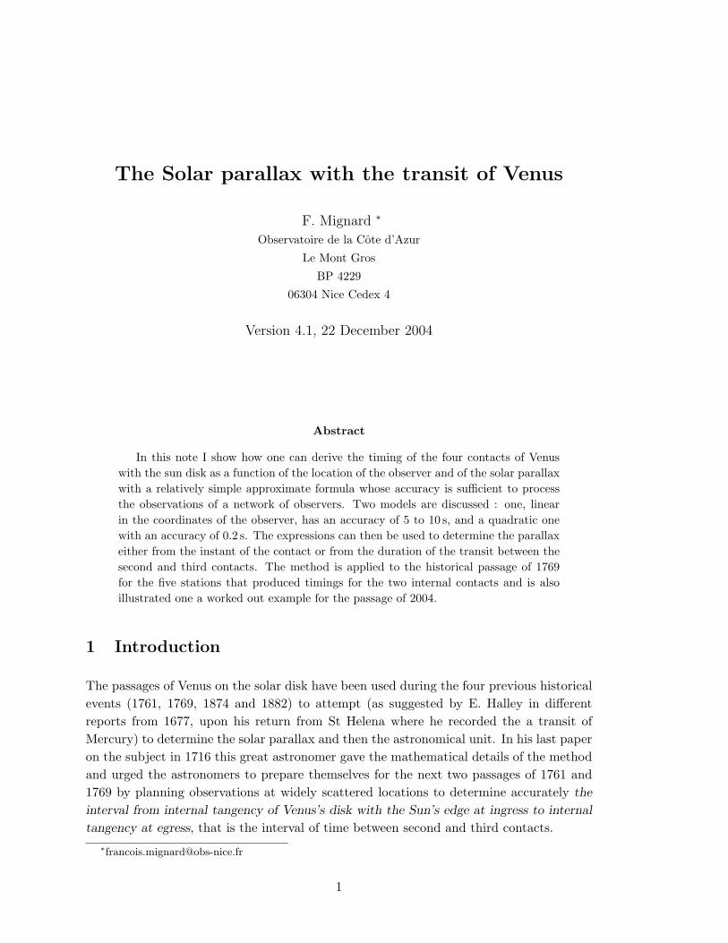
Figure 1: The four contacts of Venus during the transit on the solar disk. Only the twoinner contacts can be recorded.
2
2 Geocentric contacts
In the following one considers that the geocentric timings of the four contacts have beenpreviously computed. They have no practical importance to determine the parallax sinceone compares only the observations performed by two observers on the Earth. The geo-centric timings are common to both observers and serve only as a reference point. Theycancel out in the difference between the two actual topocentric timings.
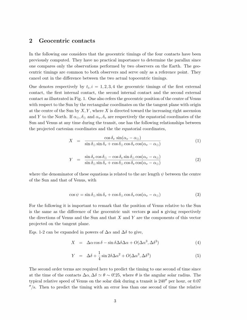
One denotes respectively by ti, i = 1, 2, 3, 4 the geocentric timings of the first externalcontact, the first internal contact, the second internal contact and the second externalcontact as illustrated in Fig. 1. One also refers the geocentric position of the centre of Venuswith respect to the Sun by the rectangular coordinates on the the tangent plane with originat the centre of the Sun by X,Y , where X is directed toward the increasing right ascensionand Y to the North. If α�, δ� and αv, δv are respectively the equatorial coordinates of theSun and Venus at any time during the transit, one has the following relationships betweenthe projected cartesian coordinates and the the equatorial coordinates,
X =cos δv sin(αv − α�)
sin δ� sin δv + cos δ� cos δv cos(αv − α�)(1)
Y =sin δv cos δ� − cos δv sin δ� cos(αv − α�)sin δ� sin δv + cos δ� cos δv cos(αv − α�)
(2)
where the denominator of these equations is related to the arc length ψ between the centreof the Sun and that of Venus, with
cosψ = sin δ� sin δv + cos δ� cos δv cos(αv − α�) (3)
For the following it is important to remark that the position of Venus relative to the Sunis the same as the difference of the geocentric unit vectors p and s giving respectivelythe directions of Venus and the Sun and that X and Y are the components of this vectorprojected on the tangent plane.
Eqs. 1-2 can be expanded in powers of ∆α and ∆δ to give,
X = ∆α cos δ − sin δ∆δ∆α+O(∆α3,∆δ3) (4)
Y = ∆δ +14
sin 2δ∆α2 +O(∆α3,∆δ3) (5)
The second order terms are required here to predict the timing to one second of time sinceat the time of the contacts ∆α,∆δ ' θ ∼ 0.◦25, where θ is the angular solar radius. Thetypical relative speed of Venus on the solar disk during a transit is 240′′ per hour, or 0.07′′/s. Then to predict the timing with an error less than one second of time the relative
3
position of the two bodies must be known to better than 0 .′′05. The second order termsin Eqs. 4 have a magnitude of θ2 ∼ 4′′ whereas the third order terms θ3 ∼ 0.′′01 can beneglected. Omitting the terms of second order may lead to an error in the timing as largeas 6 seconds of time. With a numerical program, it is advisable to keep the rigourousexpressions of Eqs. 1 instead of the power expansions.
However, in single precision, these expressions are not very good for numerical calculationas they are equivalent to compute a small arc on the sky from its cosine. So it is rec-ommended in actual programming to use the alternative and numerically more accuratefollowing expressions,
sin2 ψ
2= sin2 δv − δ�
2+ cos δv cos δ� sin2 αv − α�
2(6)
and for the numerator of Eq. 2
sin(δv − δ�) + 2 cos δv sin δ� sin2 αv − α�2
(7)
An important question arises now on a possible difference between the angular radiusof the sun at one astronomical unit defined by sin θ = R�/a where a = 1au, and theradius of the disk ρ =
√X2 + Y 2 seen projected on the tangent plane. It is easy to see
from the projection equations that ρ = tan θ. Then by neglecting the third order termsone can make ρ = θ. The error is less than 0.′′02. More generally with Eqs. 1-3 one astanψ =
√X2 + Y 2.
In this paper I have adopted the following reference values listed in Table 1 for all thenumerical computations (geocentric or topocentric).
3 Topocentric contacts
3.1 Apparent topocentric positions
An observer is located somewhere on the surface of the Earth with longitude and latitudeλ and φ where the longitude is taken positive to the east of Greenwich. When a geocentriccontact takes place, the apparent position of both Venus and the Sun are displaced fromtheir geocentric position because of the parallactic angle between the centre of the Earthand its surface. The order of magnitude is ∼ 9′′ for the Sun and at most 36′′ for Venus.The maximum relative displacement is then 28′′. Therefore, given the typical relativevelocity of Venus during a transit of 1.6 deg/day, the difference between the instants ofthe contact computed at the centre of the Earth and those observable at the surface couldbe as large as ∼ 400 seconds of time, and twice that value for the observations carried outat two nearly antipodal points on the Earth. It is time to note that the spheroidal shapeof the Earth is marginally significant to determine the contact to the nearest second. The
4
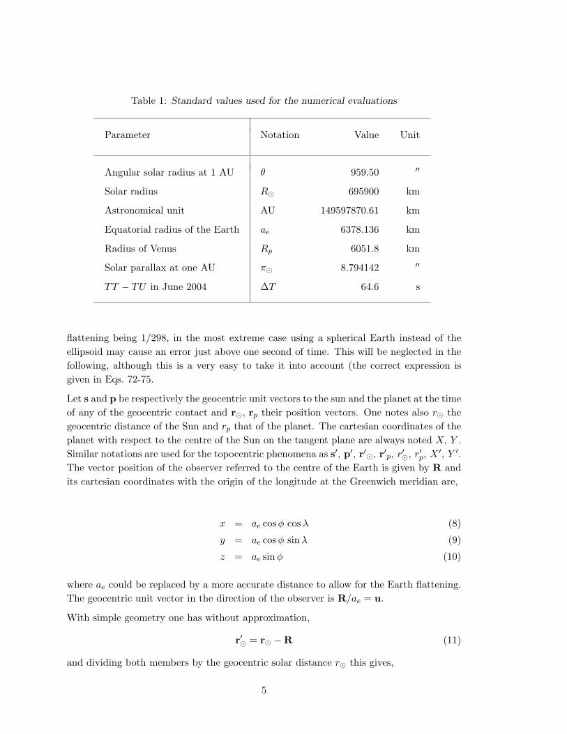
Table 1: Standard values used for the numerical evaluations
Parameter Notation Value Unit
Angular solar radius at 1 AU θ 959.50 ′′
Solar radius R� 695900 km
Astronomical unit AU 149597870.61 km
Equatorial radius of the Earth ae 6378.136 km
Radius of Venus Rp 6051.8 km
Solar parallax at one AU π� 8.794142 ′′
TT − TU in June 2004 ∆T 64.6 s
flattening being 1/298, in the most extreme case using a spherical Earth instead of theellipsoid may cause an error just above one second of time. This will be neglected in thefollowing, although this is a very easy to take it into account (the correct expression isgiven in Eqs. 72-75.
Let s and p be respectively the geocentric unit vectors to the sun and the planet at the timeof any of the geocentric contact and r�, rp their position vectors. One notes also r� thegeocentric distance of the Sun and rp that of the planet. The cartesian coordinates of theplanet with respect to the centre of the Sun on the tangent plane are always noted X, Y .Similar notations are used for the topocentric phenomena as s′, p′, r′�, r′p, r′�, r
′p, X
′, Y ′.The vector position of the observer referred to the centre of the Earth is given by R andits cartesian coordinates with the origin of the longitude at the Greenwich meridian are,
x = ae cosφ cosλ (8)
y = ae cosφ sinλ (9)
z = ae sinφ (10)
where ae could be replaced by a more accurate distance to allow for the Earth flattening.The geocentric unit vector in the direction of the observer is R/ae = u.
With simple geometry one has without approximation,
r′� = r� −R (11)
and dividing both members by the geocentric solar distance r� this gives,
5

Table 2: Useful notations
Notation Meaning
r� Geocentric position vector of the Sun
r′� Topocentric position vector of the Sun
r� Geocentric distance to the Sun
r′� Topocentric distance to the Sun
ρ� Geocentric angular radius of the Sun
s Geocentric unit vector to the Sun
s′ Topocentric unit vector to the Sun
rp Geocentric position vector of the planet
r′p Topocentric position vector of the planet
rp Geocentric distance to the planet
r′p Topocentric distance to the planet
ρp Geocentric angular radius of the planet
p Geocentric unit vector to the planet
p′ Topocentric unit vector to the planet
R Geocentric radius vector of the observer
R Distance of the observer to the Earth’s centre (∼ ae)
u Geocentric unit vector to the observer
r′�r�
= s− Rr�
(12)
To express the correspondence between the geocentric and topocentric unit vectors oneneeds to evaluate the modulus of the left-hand side of Eq. 12. Squaring both membersthis yields,
∣∣∣∣r′�r�∣∣∣∣ = (1− 2
s ·Rr�
+R2
r2�
)1/2
(13)
The second term in the above expression is of the order of the solar parallax(∼ 9′′ ∼ 10−4)whereas the last one is of the order of its square and can be neglected. This applies alsoto Venus. So to the first order in the parallax one has,
6
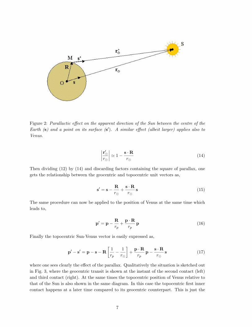
Figure 2: Parallactic effect on the apparent direction of the Sun between the centre of theEarth (s) and a point on its surface (s′). A similar effect (albeit larger) applies also toVenus.
∣∣∣∣r′�r�∣∣∣∣ ' 1− s ·R
r�(14)
Then dividing (12) by (14) and discarding factors containing the square of parallax, onegets the relationship between the geocentric and topocentric unit vectors as,
s′ = s− Rr�
+s ·Rr�
s (15)
The same procedure can now be applied to the position of Venus at the same time whichleads to,
p′ = p− Rrp
+p ·Rrp
p (16)
Finally the topocentric Sun-Venus vector is easily expressed as,
p′ − s′ = p− s−R[
1rp− 1r�
]+
p ·Rrp
p− s ·Rr�
s (17)
where one sees clearly the effect of the parallax. Qualitatively the situation is sketched outin Fig. 3, where the geocentric transit is shown at the instant of the second contact (left)and third contact (right). At the same times the topocentric position of Venus relative tothat of the Sun is also shown in the same diagram. In this case the topocentric first innercontact happens at a later time compared to its geocentric counterpart. This is just the
7

opposite for the third contact which comes earlier for the topocentric observer than at thegeocenter. In general the total duration of the phenomena will differ from place to place.
Figure 3: Schematic diagram showing the geocentric and topocentric position of Venusrelative to the centre of the Sun at the geocentric 2nd contact (left) or third contact (right).From the difference of position it is easy to evaluate the time difference between the eventsseen from different locations on the Earth and relate this difference to the solar parallax.
If we now express the distances r� and rp in astronomical units, considering a sphericalEarth and by introducing the equatorial parallax of the Sun in Eq. 17 one has,
p′ − s′ = p− s− π�
[u(
1rp− 1r�
)+
s · ur�
s− p · urp
p]
(18)
Eq. 18 is nothing but a vectorial presentation of the relative diurnal parallax between twosolar system bodies. It is convenient for the following to rewrite it as,
p′ − s′ = p− s− π�
[(1rp− 1r�
)(u− (s · u)s) +
(s · u) s− (p · u)prp
](19)
where the last term in the bracket is of the order of |s−p| ∼ the solar radius and thereforeabout 200 times smaller than the main term.
3.2 Time gap between the topocentric and geocentric phenomena
It remains now to determine the time shift between the geocentric contacts and the samecontacts observed at a particular location on the Earth surface. When Eq. 18 is evaluatedat the instant of one of the geocentric contact, one knows that the angular shift of Venusfrom the topocentric contact is of the order of the relative parallax between Venus and
8

the Sun, that is to say at most 30′′. So one needs only to evaluate the radial displacementof Venus with respect to the centre of the Sun to transform this distance into time neededto reach the contact, using in a first approximation the radial velocity of the geocentricphenomena.
The geocentric outer and inner contacts are characterised by the fact that,
|p− s| = ρ� + ρp (20)
|p− s| = ρ� − ρp (21)
expressing that the disk of Venus is tangent to that of the Sun on either side of the solaredge. For the transit of Venus of June 2004 one has typically ρ� = 945′′ and ρp = 29′′.
If one has two vectors v and v′ such that v′ = v+w and |w| � |v|, then to the first orderin w one has,
|v′| ' |v|+ v ·w|v|
(22)
or said differently, the difference of modulus is just the projection of the correction vectorto the unit initial vector.
Applying Eq. 22 to Eq. 18 one finds readily,
∣∣p′ − s′∣∣ = |p− s|− π�
|p− s|
[u · (p− s)
(1rp− 1r�
)+
(s · u) (s · (p− s))r�
− (p · u) (p · (p− s))rp
](23)
This equation is in fact much simpler than one can imagine at first glance. The first termin the bracket is like |p− s|, that is to say to sin θ, the angular radius of the Sun. Considerthe last two terms in the bracket. One has, p ·(p−s) = 1−p ·s and s ·(p−s) = −(1−p ·s).With p · s = cos(θ), the factors are like 1 − cos θ ∼ θ2 and about 200 times smaller thanthe main term. Then one can take p · u ∼ s · u, meaning that one identifies the zenithdistance of Venus to that of the centre of the Sun. Finally we can rewrite Eq. 23 as,
∣∣p′ − s′∣∣ = |p− s| − π�
|p− s|
[u · (p− s)
(1rp− 1r�
)− (s · u) (1− p · s)
(1rp
+1r�
)](24)
The first term in the bracket will produce time shifts as large as 400 s while the secondwill never add corrections larger than 2 seconds of time. But as both are linear in thesolar parallax and in the position vector of the observer, there is no reason not to includethem simultaneously.
The last step is now to compute the radial velocity of Venus on the Solar disk at eachcontact. Let w the transit velocity, that is to say the vector of components X, Y on the
9

projection plane. These components are computed at each geocentric contact and arenumerical values for a particular transit. The radial velocity is then ,
wr =w · (p− s)|p− s|
(25)
or
wr =XX + Y Y
ρ� ± ρp(26)
where the± refers to the external or internal contacts. Combining 24 and 25 one eventuallyobtains the time of the topocentric contacts from the corresponding geocentric timings.
t′i = ti + τ(1)i + τ
(2)i (27)
with i = 1..4, where τ (1) and τ (2) denotes respectively the main and secondary terms from(24).
One gets,
τ (1) = π�
[u · (p− s)w · (p− s)
(1rp− 1r�
)](28)
and
τ (2) = −π�[(u · s)(1− p · s)
w · (p− s)
(1rp
+1r�
)](29)
Remarks about the units : The derivation assumes that all the angles, including thesolar parallax, are in radians and the velocity in radian per unit of time. Care must betaken in the numerical evaluation mixing radians, degrees and arcseconds to ensure thehomogeneity of the angular terms in the numerator and denominator. For example themagnitude of (28) is essentially π�/|w|(1/rp − 1/r�). With |w| ∼ 1.6 deg/day, one mustexpress π� in degrees, to obtain τ (1) ∼ 400 s.
If we limit the evaluation to τ (1) we can draw interesting conclusions from simple argu-ments :
• For a particular contact, all the vectors but u of Eq. 28 are known and do not dependon the observer. Putting for the unit vector u,
α = cosφ cosλ
β = cosφ sinλ (30)
γ = sinφ
we see that once reduced in numbers, assuming a known solar parallax, τ (1) willreduce to
10

Aα+Bβ + Cγ (31)
where A, B, C will depend only on the contact. In addition these coefficients aredirectly proportional to the solar parallax.
• From (31) or directly from the scalar product in (28) one sees that τ (1) = Γ× cosψwhere ψ is the angle between u and an axis parallel to p− s and going through thecentre of the Earth with Γ = (A2 + B2 + C2)1/2. Therefore the difference betweenthe timing of the geocentric contact and the topocentric timings goes from +Γ to -Γand is zero for observers located in a plane normal to p− s.
• The difference of the duration of the phenomena (topocentric - geocentric) betweenthe second and the third contact will be given by,
(A3 −A2)α+ (B3 −B2)β + (C3 − C2)γ (32)
having then the same form as for either contacts. So one can also define an axis onthe Earth so that τ3 − τ2 = Γ cosψ. This remarkable property will be essential toassess the solar parallax from observations performed at two or more locations.
3.3 Practical formulas
The various scalar products can be evaluated in the most convenient frame. The positionof the observer is naturally known in a frame tied to the rotating Earth with the originof longitude at the Greenwich meridian. The components of the vector p − s are knownin cartesian coordinates in the plane tangent to the celestial sphere in the direction of theSun. The coordinates X, Y are given for each contact by Eqs. 1 or 4.
In the local frame attached to the centre of the Sun on has,
p− s =
0X
Y
(33)
Let H� be the hour angle of the Sun for the Greenwich meridian at one of the contacts(omitting the subscript i to label the contact) and δ� its declination. Therefore the matrixthat transforms the components of a vector from the local tangent frame into the hoursystem is given by the application of two rotations,
R3(H�)R2(δ�) =
cosH� cos δ� sinH� − cosH� sin δ�− sinH� cos δ� cosH� sinH� sin δ�
sin δ� 0 cos δ�
(34)
11

Figure 4: Relationship between the local reference frame on the tangent plane centered atthe Sun and the hour system with the Greenwich meridian for the origin of the longitudesand the hour angles. The close-up on the right is viewed from inside the celestial sphere.
Thus one has in the hour frame,
p− s =
X sinH� − Y cosH� sin δ�X cosH� + Y sinH� sin δ�
Y cos δ�
(35)
which leads to,
τ (1) = A cosφ cosλ+B cosφ sinλ+ C sinφ (36)
with
A =π�
XX + Y Y
[1rp− 1r�
](X sinH� − Y cosH� sin δ�) (37)
B =π�
XX + Y Y
[1rp− 1r�
](X cosH� + Y sinH� sin δ�) (38)
C =π�
XX + Y Y
[1rp− 1r�
](Y cos δ�) (39)
We have also
12
τ (2) = δA cosφ cosλ+ δB cosφ sinλ+ δC sinφ (40)
where the only vector to be expressed in the hour frame is s,
s =
cos δ� cosH�
− cos δ� sinH�
sin δ�
(41)
giving
δA = − 2π�XX + Y Y
sin2 θ
2
[1rp
+1r�
]cos δ� cosH� (42)
δB =2π�
XX + Y Ysin2 θ
2
[1rp
+1r�
]cos δ� sinH� (43)
δC = − 2π�XX + Y Y
sin2 θ
2
[1rp
+1r�
]sin δ� (44)
As mentioned earlier the coefficients A, B, C are of the order of few hundred seconds whilethe δA, δB, δC reach only one or two seconds of time. From comparisons with rigourousestimates of the topocentric phenomenons for various locations, I estimate the accuracy ofthe prediction of the topocentric contacts with the approximate formulas to better than0.1 minute of time at most locations, with maximum departure of 10-15s at some places.This is sufficient to process observational material, given the difficulties to ascertain theinstant of the contacts even within 10 seconds. For the best observations, more accurateexpressions (but also more intricate) derived in the next sections may be needed.
4 Further refinements
4.1 Statement of the problem
It is shown later in this note that the accuracy of the linear formula for the instant ofthe topocentric contacts is in general better than 10 seconds, with a well defined patternas a function of the location. It is also found that the errors for any of the four contactsdoes not average out over the earth when locations are picked uniformly distributed, afeature not accounted for by the linear formula. The relatively poor performances of thelinear approximation is rather surprising and not intuitive, since the main approximationcomes from neglecting the square of the parallax in Eq. 18. As the difference between thegeocentric and topocentric contacts is at most ∆τ ∼ 500s, one expects the neglect termsto be of the order of π� ∆τ ∼ 0.05 s and not the 5–10 s eventually found.
This unaccounted discrepancy is both puzzling and challenging. It must be investigated,at least to understand its origin and possibly to produce a better formula. There are
13

clearly second order terms missing, larger than simply those that would come directlyfrom π2
� in the parallactic equation and unrelated to them. I eventually found the culprithidden away in a dark corner.
If we look again at Eq. 18 one sees that the parallactic term is small compared to p−s andnot relative to the unit vectors p or s, as it was the case in Eqs. 15-16. As |p−s| ∼ θ�, thesecond order terms is typically π�/θ� ∼ 0.01 smaller than the main term and not simplyπ� ∼ 10−4 . This means that some second order terms in the derivation of ∆τ will be ofthe order of ∼ 5 s, instead of 0.05 s, and this will happen even with the parallactic equationlimited to first order in π�. This difference of few seconds is precisely the accuracy of thelinear formula found from a comparison to a full numerical computation of the contacts.One then needs to recompute the topocentric timings by allowing for these second orderterms.
4.2 Second order equations
As explained there is no need at this point to introduce the square of the parallax in thebasic equations (18) or (19). The problem can then be restated as follows : given thetopocentric position of Venus relative to the Sun as,
p′ − s′ = p− s− π�
[(1rp− 1r�
)(u− (s · u)s) +
(s · u) s− (p · u)prp
](45)
and knowing the geocentric motion of the two bodies and that of the observer, one wishesto solve for the time t the equations,
|p′(t)− s′(t)| = ρ� ± ρp (46)
The solutions of (46) will be the instant of the four topocentric contacts and it must beobtained with a better accuracy than that of the linear model. We also assume that thesolution for the geocentric contacts is known, meaning that at for certain t0,
|p(t0)− s(t0)| = ρ� ± ρp (47)
has been solved. To avoid too many subscripts, the contacts are not indexed here and theformulas are meant to apply to any of the four contacts. For brevity one puts hereafterv = p− s and v′ = p′ − s′ and introduce 1/p = 1/rp − 1/r� for the parallactic factor. Inthis discussion one can restrict the parallactic equation (45) to its simplest form,
v′ = v − π�p
[u− (s · u)s] (48)
14

since we have already shown that the additional terms give corrections of the order of∼ 1 s (29) and that they will not interfere with the second order terms we are about toderive.
Let t0 the time of a geocentric contact and ρ the distance to the center of the Sun (so ρis either ρ� + ρp or ρ� − ρp according to the contact). At this time
v2(t0) = ρ2 (49)
(the equations are easier to derive with the square of the distance). The same contact foran Earth-based observer occurs at t with
v′2(t) = ρ2 (50)
Now with (48)
v′2 = v2 − 2π�p
u · v +π2�p2
[1− (s · u)2
](51)
and by inserting the geocentric contact, the equation for the time of the topocentric contactreduces to,
v2(t)− v2(t0)− 2π�p
u · v +π2�p2
[1− (s · u)2
]= 0 (52)
This equation is very general and the only approximation results from our neglecting π2�
in the initial parallactic equation. As mentioned earlier this does not conflict with thesecond order terms of (52), since the magnitude of the second order term relative to thefirst order is π�/|v| ∼ 0.01 and not π� ∼ 10−4.
In the vicinity of the contact the geocentric motion of Venus relative to the Sun is nicelyapproximated by a rectilinear uniform motion as,
v(t) = v(t0) + w τ (53)
and the motion of the observer is provided by the rotation of the Earth as,
u(t) = u(t0) + ω × u(t0) τ (54)
where ω is the rotation vector of the Earth and τ = t− t0. Inserting in (52) this leads to,
π�p
u · v − 12π2�p2
[1− (s · u)2
]−[v ·w − π�
p(ω × u) · v − π�
pu ·w
]τ − 1
2w2τ2 = 0 (55)
15

Although this quadratic equation in τ can be solved in closed form it is better to usethe fact that τ ∼ π�/|w| to solve the linear part first and add the quadratic term as acorrection. After few algebraic transformations one gets,
τ =π�p
u · vw · v
(56)
+π2�p2
[(u · v)((ω × u) · v)
(w · v)2+
(u · v)(u ·w)(w · v)2
− 12
[1− (s · u)2
]w · v
− 12
(w ·w)(u · v)2
(w · v)3
]
where the first order term is the same as (28). The complementary expression (29) doesnot appear as expected since I have discarded the specific small terms in the parallacticequation (48). So Eq. 29,
τ (2) = −π�[(u · s)(1− p · s)
w · v
(1rp
+1r�
)](57)
should be added to this result to get the correct timing to the second order.
It is interesting to rewrite (56) by introducing,
Γ = (A,B,C)T =π�p
vw · v
(58)
where the components A, B, C are the same as in (37). Put also,
Γ′ = (A′, B′, C ′)T =π�p
ww · v
(59)
Then (56) becomes,
τ = Γ · u + (Γ · u) [Γ · (ω × u)] + (Γ · u) (Γ′ · u) (60)
−12π2�p2
[1− (s · u)2
]w · v
− 12
(w ·w)(w · v)
(Γ · u)2
With this last equation the question raised at the beginning of this section is answered,since we have now a solution for the time of the contacts including second order terms. Aquick evaluation of each term with u2 indicates that they are all of the order of 1 to 5 s,as expected.
16

Table 3: Coefficients of the expansion of (60) on the spherical functions.
Term Γ · u (Γ · u) [Γ · (ω × u)] (Γ · u) (Γ′ · u) (Γ · u)2 1− (s · u)2
C00 0 0 (AA′ + BB′ + CC′)/3 (A2 + B2 + C2)/3 2/3
C11 A 0 0 0 0
S11 B 0 0 0 0
C10 C 0 0 0 0
C22 0 AB/3 (AA′ −BB′)/6 (A2 −B2)6 (S2y − S2
x)/6
S22 0 (B2 −A2)/6 (AB′ + BA′)/6 AB/3 −SxSy/3
C21 0 BC/3 (AC′ + CA′)/6 2AC/3 −2SxSz/3
S21 0 −AC/3 (BC′ + CB′)/6 2BC/3 −2SySz/3
C20 0 0 −(AA′ + BB′ − 2CC′)/3 −(A2 + B2 − 2C2)/3 (1− 3S2z )/2
4.3 Convenient representation
It appears from these equations that the time difference between the geocentric andtopocentric contacts can be expressed as a function of the location of the observer with anexpansion involving only first and second degree of u. A full expansion of (56) will leadto a second degree polynomial in α, β, γ. So it is possible to derive a certain number ofconstants, depending only on the transit and the contacts but not on the observer, fromwhich any timing could be computed for a particular location. We have already done thisexpansion with the linear term in u and it is wise to organise the expansion to the secondorder on the spherical functions of the first and second degree. Our previous expansionturns out to be identical to such a development on the spherical function of first ordersince,
C11 = cosφ cosλ = α
S11 = cosφ sinλ = β
C10 = sinφ = γ
(61)
Now more generally one has,
17

C00 = 1C22 = 3 cos2 φ cos 2λ = 3(α2 − β2)S22 = 3 cos2 φ sin 2λ = 6αβC21 = 3 cosφ sinφ cosλ = 3αγS21 = 3 cosφ sinφ sinλ = 3βγC20 = (3 sin2 φ− 1)/2 = (3γ2 − 1)/2
(62)
There are in total only nine base functions, since α2+β2+γ2 = 1. It remains to expand (60)on α, · · · , α2, · · · , αβ · · · and then on the Clm, Slm to obtain a general formula applicableto any locations. For the user the nine numerical values for each contact can be computedin advance and provided in the form of table. The analytical form of the contribution ofeach second order factor of (60) is given in Table 3. One must note in this table that thefirst line gives the average of the difference between the topocentric and geocentric timingover the Earth. For the 2004 Venus transit the numerical values are listed in Tables 5 and6.
Table 4: Venus transit of 8 June 2004 – Geocentric contacts
Contact Time X Y X Y θ H�
UT ′′ ′′ ′′/h ′′/h ′′ deg
1st 05h13m34s 873.44 -431.34 -233.62 -57.35 945.40 258.62
2nd 05h32m51s 798.41 -449.76 -233.62 -57.35 945.39 263.45
3rd 11h06m41s -501.99 -766.61 -233.80 -56.53 945.37 -13.10
4th 11h25m58s -577.09 -784.78 -233.80 -56.53 945.37 -8.28
5 Numerical Values
5.1 The geocentric transit
The circumstances of the Venus transit of June 2004 have been computed with the referencevalues listed in Table 1 and solar system ephemeris developed over the years at the Institutde Mecanique Celeste et de Calcul des Ephemerides in Paris. The timings are computedin dynamical times but given as usual in UT, using TT − UT = 64.6s in June 2004. Thisvalue may differ by few seconds from one institute to another and will be known for sure atthe end of 2004. The predictions are also very sensitive to the solar radius : increasing this
18
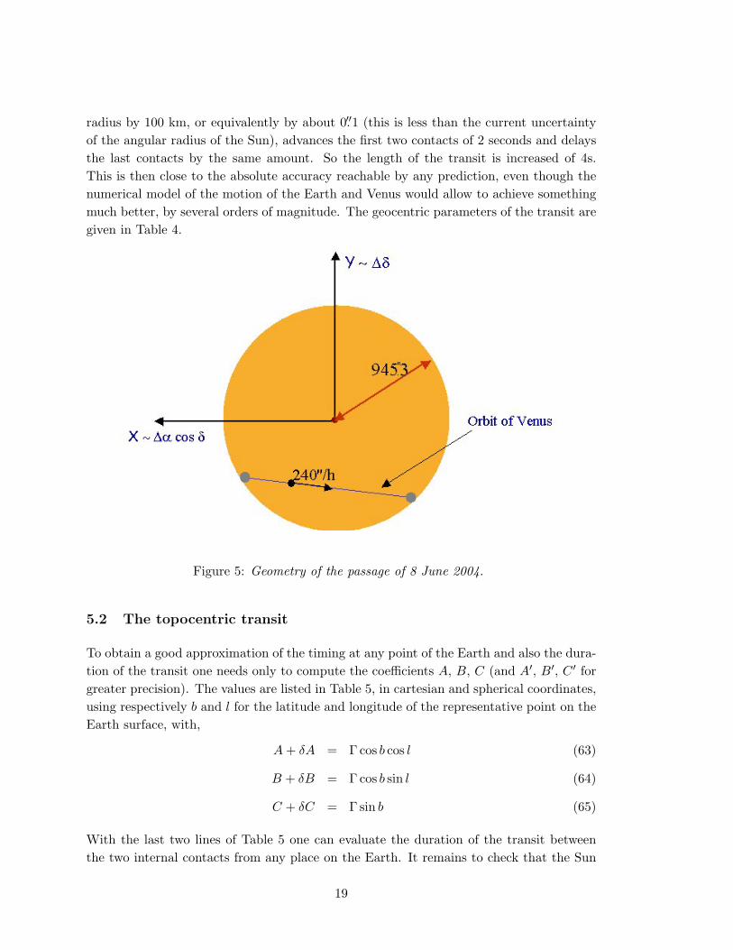
radius by 100 km, or equivalently by about 0.′′1 (this is less than the current uncertaintyof the angular radius of the Sun), advances the first two contacts of 2 seconds and delaysthe last contacts by the same amount. So the length of the transit is increased of 4s.This is then close to the absolute accuracy reachable by any prediction, even though thenumerical model of the motion of the Earth and Venus would allow to achieve somethingmuch better, by several orders of magnitude. The geocentric parameters of the transit aregiven in Table 4.
Figure 5: Geometry of the passage of 8 June 2004.
5.2 The topocentric transit
To obtain a good approximation of the timing at any point of the Earth and also the dura-tion of the transit one needs only to compute the coefficients A, B, C (and A′, B′, C ′ forgreater precision). The values are listed in Table 5, in cartesian and spherical coordinates,using respectively b and l for the latitude and longitude of the representative point on theEarth surface, with,
A+ δA = Γ cos b cos l (63)
B + δB = Γ cos b sin l (64)
C + δC = Γ sin b (65)
With the last two lines of Table 5 one can evaluate the duration of the transit betweenthe two internal contacts from any place on the Earth. It remains to check that the Sun
19

Table 5: Venus transit of June 2004. Coefficients for the topocentric contacts : linear
formula.
Contact A+ δA B + δB C + δC Γ b l
s s s s deg deg
1st 388.6 4.9 174.4 425.9 24.2 0.7
2nd 396.5 -38.6 202.9 447.0 27.0 354.4
3rd 195.5 -206.0 -345.3 447.1 -50.6 313.5
4th 166.9 -230.7 -316.8 426.0 -48.1 305.9
2nd to 3rd -200.9 -167.4 -548.2 607.3 -64.5 219.8
1st to 4th -221.6 -235.7 -491.2 588.2 -56.6 226.8
is above the horizon at this time. However the result of the computation is preciselywhat would be observed through a transparent Earth if the sun is set !. The accuratevalue of the difference between the topocentric and geocentric time of the contacts andthe duration of the inner transit is plotted in Fig. 6 for any point on the Earth, lettingaside the problem of visibility. The plots show obvious pattern of regularity with themaximum deviation around the poles indicated in Table 5. The model with 3 (linear) or9 (quadratic) parameters aims precisely to account for this pattern.
5.3 Accuracy of the approximation
Earlier in this note I have estimated the accuracy of the simplified formula to 5–10 s,without providing hints for the magnitude of the neglected terms. This was based onquick comparison between predictions based on the linear model and a rigourous numericalcomputation of the time of the contacts. About the accuracy one must already notice thatthe various official, and basically very trustworthy, computations carried out in Paris,Washington or by Nasa, may differ by few seconds in the geocentric phenomena. Thiscomes primarily, not from the model as stated earlier, but from the adopted angularradius of the Sun, from the prediction of the rotation of the Earth in June 2004, and toa lesser extent to the ephemerides they use. Therefore a precision of one second, is notonly not required for the observations, but is difficult to achieve in absolute sense withour knowledge of the solar diameter.
20
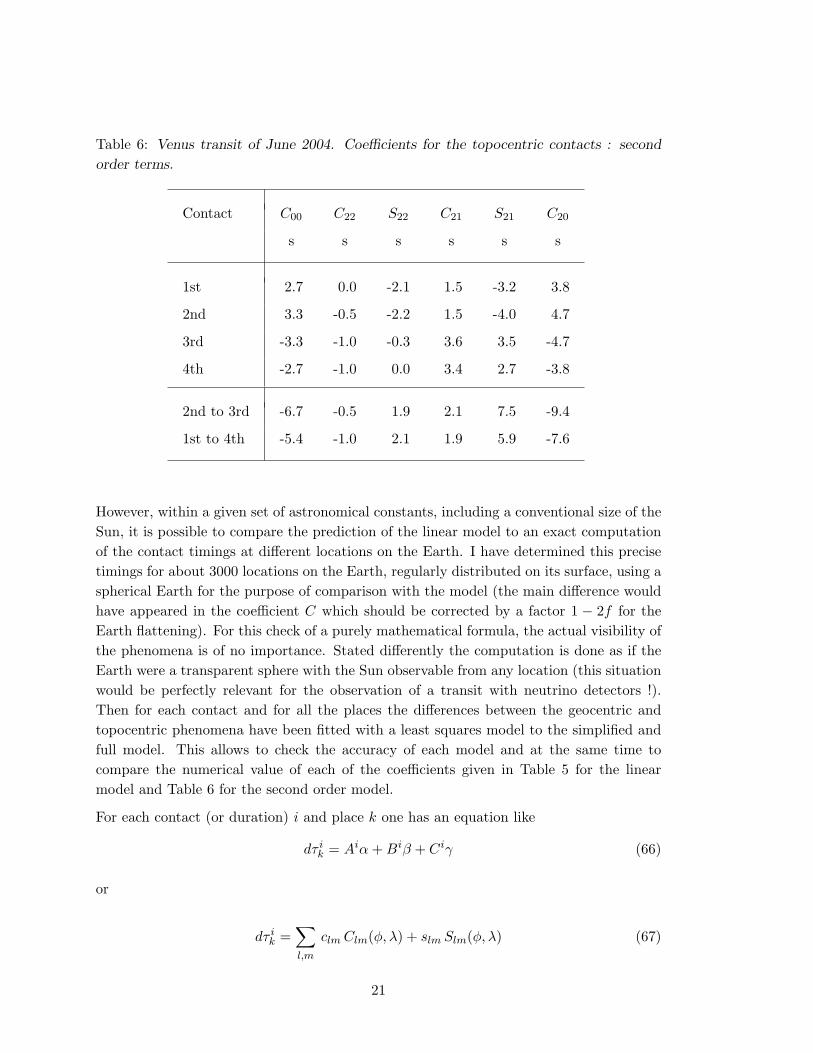
Table 6: Venus transit of June 2004. Coefficients for the topocentric contacts : second
order terms.
Contact C00 C22 S22 C21 S21 C20
s s s s s s
1st 2.7 0.0 -2.1 1.5 -3.2 3.8
2nd 3.3 -0.5 -2.2 1.5 -4.0 4.7
3rd -3.3 -1.0 -0.3 3.6 3.5 -4.7
4th -2.7 -1.0 0.0 3.4 2.7 -3.8
2nd to 3rd -6.7 -0.5 1.9 2.1 7.5 -9.4
1st to 4th -5.4 -1.0 2.1 1.9 5.9 -7.6
However, within a given set of astronomical constants, including a conventional size of theSun, it is possible to compare the prediction of the linear model to an exact computationof the contact timings at different locations on the Earth. I have determined this precisetimings for about 3000 locations on the Earth, regularly distributed on its surface, using aspherical Earth for the purpose of comparison with the model (the main difference wouldhave appeared in the coefficient C which should be corrected by a factor 1 − 2f for theEarth flattening). For this check of a purely mathematical formula, the actual visibility ofthe phenomena is of no importance. Stated differently the computation is done as if theEarth were a transparent sphere with the Sun observable from any location (this situationwould be perfectly relevant for the observation of a transit with neutrino detectors !).Then for each contact and for all the places the differences between the geocentric andtopocentric phenomena have been fitted with a least squares model to the simplified andfull model. This allows to check the accuracy of each model and at the same time tocompare the numerical value of each of the coefficients given in Table 5 for the linearmodel and Table 6 for the second order model.
For each contact (or duration) i and place k one has an equation like
dτ ik = Aiα+Biβ + Ciγ (66)
or
dτ ik =
∑l,m
clmClm(φ, λ) + slm Slm(φ, λ) (67)
21

Figure 6: Difference in seconds between the geocentric and topocentric time of the second(top) and third contact (middle), and difference of duration of the transit (bottom) forany point on the Earth (irrespective of the visibility). The plot is based on a rigorouscomputation for the contacts of the 2004 transit.
22

according to the model.
The results are shown in Table 7 (linear model) Table 8 (full model) for the second andthird contact and for the duration of the transits between these contacts.
A straight comparison with Tables 5-6, confirms that the analytic modelling and thenumerical evaluation of the coefficients are correct, and that not term of second orderis missing. The remaining difference between the coefficients is less than 0.1 s. The lasttwo columns give the average of the post-fit residuals and their standard deviation. Asmentioned earlier, the linear model leaves residuals between 5 and 10 s, which do notaverage out over the Earth. The standard deviation is about 5 s for the contacts and 8sfor the duration. Results are exactly similar for the first and fourth contact.
Table 7: Venus transit of June 2004 : Coefficients for the topocentric contacts fitted with
the linear model onto an accurate determination of the contacts on uniformly sampled
points on the Earth.
Contact A+ δA B + δB C + δC Mean σ
s s s s s
2nd 396.4 -38.6 203.0 3.4 5.2
3rd 195.5 -205.8 -345.4 -3.3 4.7
2nd to 3rd -200.9 -167.2 -548.5 -6.6 8.0
The distribution of the residuals is shown in Fig. 7 (linear model) and 8 (second ordermodel) for the duration between the second and third contact. In the first case we see avery distinctive pattern as a function of the longitude and latitude with a non-zero averageover the surface of the Earth. The amplitudes around the mean have a maximum of 10seconds for the contacts and 15s for the duration of the transit and the standard deviationsare respectively 5 and 8 seconds, that is to say in keeping with the claim of an accuracyof 0.1 mn for the linear formula. When the full model is applied the residuals are down byalmost two orders of magnitude, and the remaining effect averages out to zero althoughthe remaining residuals are not yet pure noise. However there is neither theoretical norpractical need to derive a more accurate analytical formula than (56) for the timings.
23

Table 8: Venus transit of June 2004 : Coefficients for the topocentric contacts fitted with
the complete model onto an accurate determination of the contacts on uniformly sampled
points on the Earth.(The coefficients of the linear model are not repeated)
Contact C00 C22 S22 C21 S21 C20 Mean σ
s s s s s s s s
2nd 3.4 -0.4 -2.2 1.5 -4.0 4.7 0 0.14
3rd -3.3 -1.0 -0.3 3.6 3.5 -4.7 0 0.11
2nd to 3rd -6.6 -0.5 1.9 2.1 7.5 -9.4 0 0.19
24

Figure 7: Residuals in seconds for the 2004 Venus transit in the timing of the second (top)and third contact (middle) and the transit duration (bottom) between the exact computationand the linear model with three coefficients using the best fitted values of Table 7, for anypoint on the Earth (irrespective of the visibility). Note the amplitude of ∼ 10 s and thenon zero average.
25

Figure 8: Residuals in seconds for the 2004 Venus transit in the timing of the second(top) and third contact (middle) and the transit duration (bottom) and between the exactcomputation and the second order model with nine coefficients using the best fitted valuesof Table 8, for any point on the Earth. The amplitude is less than 0.5 s and the averageis zero.
26
6 Determination of the solar parallax
In this section an application of the linear model is proposed in view of processing timingsto determine the astronomical unit. As explained in the previous sections the time differ-ence between the geocentric and topocentric contacts is given by the simple expression,
τ = Aα+Bβ + Cγ (68)
where A, · · · stands in fact for A + δA, · · · and α, β, γ are the direction cosines of theobserver referred to the equator and the Greenwich meridian with,
α = cosφ cosλ (69)
β = cosφ sinλ (70)
γ = sinφ (71)
If one wishes to allow for the flattening of the Earth this must be replaced by,
α = ρ(φ) cosφ cosλ (72)
β = ρ(φ) cosφ sinλ (73)
γ = ρ(φ)(1− 2f) sinφ (74)
with,
ρ(φ) = (1− 2f sin2 φ)−1/2 (75)
where f = 1/298.26 is the Earth flattening (relative difference between the equatorial andpolar radius). The effect of the flattening on the timing will be at most of 1 to 2 secondsof time.
6.1 Parallax from the timings
All the numerical values in Table 5 have been computed with an assumed solar parallaxπref = 8.794142, that is to say an astronomical unit of 149597870.61 km. The coefficientsA, · · · are directly proportional to π�.
Let two distant observers located at coordinates φ1, λ1 and φ2, λ2. Assuming that theirclocks are perfectly set and that they can express their measurements in UTC, the expectedcontact timings of the ith contact for the first observer is,
27
t(i)1 = t
(i)geo + Aα1 + Bβ1 + Cγ1 (76)
where t(i)geo is the geocentric time of the contact. For the second observer one has a similarequation,
t(i)2 = t
(i)geo + Aα2 + Bβ2 + Cγ2 (77)
Therefore by subtracting these two equations one gets the expected timing difference forthese two observers as,
dtc = A(α2 − α1) + B(β2 − β1) + C(γ2 − γ1) (78)
where the coefficients are taken for the relevant contact(s) in Table 5. If they measure adifference dto, and if the only source of discrepancy is the value of the solar parallax, thenthey can conclude that the true value of the solar parallax is,
π� = πrefdtodtc
(79)
6.2 Parallax from the duration of the transit
6.2.1 Two observers
The comparison between observers of the duration of the transit between the secondand third contact, is much easier as it requires only a good standard wristwatch at eachlocation to assess a duration of few hours to few seconds accuracy. Therefore each observerdetermines a duration and can dispense with an accurate synchronisation to some form ofUT. The formula for the computed value is the same as (78) with the coefficients A, . . .taken from the last line of Table 5. As before, if they observed a difference of durationdto, they can conclude from this single pair of measurements a value of the parallax withEq. 79.
It is important to stress that the reference value of the parallax is totally irrelevant and thatonly the precision of the observations performed at the two locations matters. Changingthe reference parallax would change the coefficients A, · · · accordingly and would not affectthe ratio πref/dtc.
6.2.2 Combination of observations
Having n observers on the Earth able to observe ingress and egress providesN = n(n−1)/2baselines and as many different determinations of parallaxes. Even if each observer worked
28

Table 9: Topocentric coefficients for the historical Venus transits for the duration be-
tween the two inner contacts. The second column gives the computed geocentric duration
between this two contacts. The reference parallax π� = 8.′′794142 has been used.
Year t3 − t2 A B C
s s s
1761 05h57m41s 4.6 -313.4 -465.6
1769 05h42m12s 476.5 376.5 516.1
1874 03h36m38s -293.1 -12.9 1178.6
1882 05h39m03s -302.1 591.9 -576.1
with the same accuracy in the timing of the contacts, the precision on the parallaxes wouldnot be constant. A longer baseline (in fact a longer shift in the duration of the transitbetween the two locations) yields a more accurate parallax. Therefore one cannot combinestraightforwardly the N determinations into a single one without weighing properly eachdetermination. The weight is a function of the accuracy of the individual timings (verydifficult to assess) and of the baseline. Once this is done, one must evaluate the standarderror, taking into account that if there are N parallaxes, there are not N independentmeasurements, but only n. Thus a full N × N correlation matrix must be evaluatedto assess the final standard error. The details are given in the next section with theapplication to the transit of 1769.
7 Application to the passage of 1769
The method developed in the previous sections can be applied to the historical transits,in particular that of 1769 when combined measurements of the inner and outer contactshave been obtained at different locations. For these transits the relevant coefficients forthe topocentric durations between the 2nd and 3rd contact are given in Table 9.
Consider now the observations performed during the expeditions of 1769, restricting to thefive stations where the two internal contacts of Venus with the Sun where properly seenand timed. A very simple approach consists of grouping the stations two by two so thatone parallax can be estimated for each of the possible pairs. Clearly the results are notstatistically independent and this would not be the method favoured today by astronomers,but basically this was the method employed in the XVIIIth century. The first two stationsbeing very similar in position I will not combine them as a pair, although they would
29
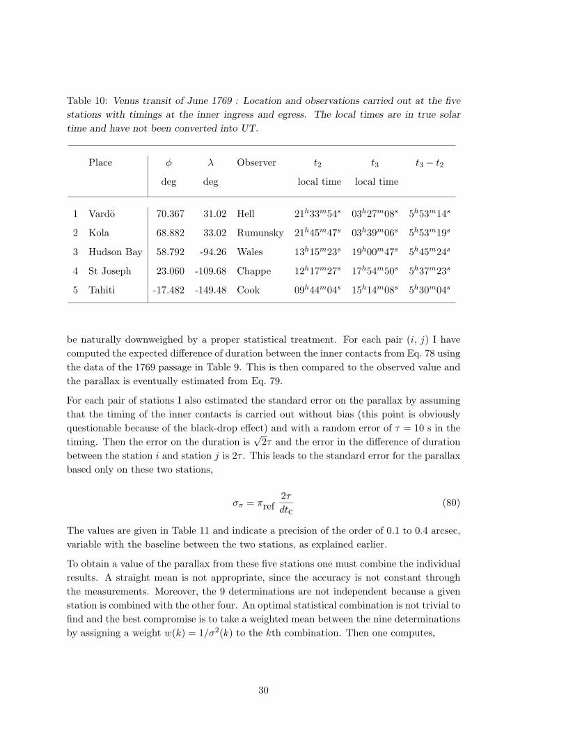
Table 10: Venus transit of June 1769 : Location and observations carried out at the five
stations with timings at the inner ingress and egress. The local times are in true solar
time and have not been converted into UT.
Place φ λ Observer t2 t3 t3 − t2
deg deg local time local time
1 Vardo 70.367 31.02 Hell 21h33m54s 03h27m08s 5h53m14s
2 Kola 68.882 33.02 Rumunsky 21h45m47s 03h39m06s 5h53m19s
3 Hudson Bay 58.792 -94.26 Wales 13h15m23s 19h00m47s 5h45m24s
4 St Joseph 23.060 -109.68 Chappe 12h17m27s 17h54m50s 5h37m23s
5 Tahiti -17.482 -149.48 Cook 09h44m04s 15h14m08s 5h30m04s
be naturally downweighed by a proper statistical treatment. For each pair (i, j) I havecomputed the expected difference of duration between the inner contacts from Eq. 78 usingthe data of the 1769 passage in Table 9. This is then compared to the observed value andthe parallax is eventually estimated from Eq. 79.
For each pair of stations I also estimated the standard error on the parallax by assumingthat the timing of the inner contacts is carried out without bias (this point is obviouslyquestionable because of the black-drop effect) and with a random error of τ = 10 s in thetiming. Then the error on the duration is
√2τ and the error in the difference of duration
between the station i and station j is 2τ . This leads to the standard error for the parallaxbased only on these two stations,
σπ = πref2τdtc
(80)
The values are given in Table 11 and indicate a precision of the order of 0.1 to 0.4 arcsec,variable with the baseline between the two stations, as explained earlier.
To obtain a value of the parallax from these five stations one must combine the individualresults. A straight mean is not appropriate, since the accuracy is not constant throughthe measurements. Moreover, the 9 determinations are not independent because a givenstation is combined with the other four. An optimal statistical combination is not trivial tofind and the best compromise is to take a weighted mean between the nine determinationsby assigning a weight w(k) = 1/σ2(k) to the kth combination. Then one computes,
30

Table 11: Venus transit of June 1769 : Estimation of the solar parallax from the combi-
nation of observing stations with the timings of the 2nd and 3rd contacts. The estimate
of the standard error is based on a random timing error of 10 s at each contact.
] Combination dtc dtobs π� σ AU
s s ′′ ′′ 106 km
1 1 - 3 461 470 8.96 0.4 146.8
2 1 - 4 961 951 8.70 0.2 151.2
3 1 - 5 1418 1390 8.62 0.1 152.6
4 2 - 3 472 475 8.84 0.4 148.8
5 2 - 4 973 956 8.64 0.2 152.3
6 2 - 5 1430 1395 8.58 0.1 153.3
7 3 - 4 500 481 8.45 0.4 155.7
8 3 - 5 957 920 8.45 0.2 155.7
9 4 - 5 457 439 8.44 0.4 155.9
π� =9∑
k=1
w(k)π(k)/∑
w(k) = 8.′′61 (81)
The standard error of this weighted mean can be estimated from the variance of (81),by taking into account the correlations between the different observations. It is easyto establish that the correlation coefficient ρ(k, k′) between the results k based on thecombination from the stations (i, j) and k′ for the stations (i′, j′) is 0, if there are nostations in common, 1/2 for the combinations (i, j) with (i, j′) or (i, j) with (i′, j) and-1/2 for the combinations (i, j) with (j′, i) or (i, j) with (j, i′). The simple structure ofthe correlations matrix comes also from the uniform error in the timing (τ = 10 s) assumedfor each observer.
For the nine combinations of Table 11 the correlation matrix has the following form,
31

1
2
3
4
5
6
7
8
9
1.0 0.5 0.5 0.5 0.0 0.0 −0.5 −0.5 0.0
0.5 1.0 0.5 0.0 0.5 0.0 0.5 0.0 −0.5
0.5 0.5 1.0 0.0 0.0 0.5 0.0 0.5 0.5
0.5 0.0 0.0 1.0 0.5 0.5 −0.5 −0.5 0.0
0.0 0.5 0.0 0.5 1.0 0.5 0.5 0.0 −0.5
0.0 0.0 0.5 0.5 0.5 1.0 0.0 0.5 0.5
−0.5 0.5 0.0 −0.5 0.5 0.0 1.0 0.5 −0.5
−0.5 0.0 0.5 −0.5 0.0 0.5 0.5 1.0 0.5
0.0 −0.5 0.5 0.0 −0.5 0.5 −0.5 0.5 1.0
Then we have for the standard deviation of the weighted mean,
σ2π� =
(9∑
k=1
w(k)2σ2(k) + 2∑
k
∑k′>k
w(k)w(k′) ρ(k, k′)σ(k)σ(k′)
)/(∑
w(k))2
(82)
yielding the final result,
π� = 8.61± 0.10 (83)
(If the correlations are omitted the standard error is only 0.′′06). This result is in goodagreement with the extensive and numerous discussions that followed the transit of 1761,whose final conclusion was a solar parallax between 8.′′45 and 8.′′85 and the re-evaluationson the XIXth century by Encke in 1824 leading to π� = 8.′′6030.
8 Worked example for the passage of 2004
This section summarises the results developed in detail in the course of this paper, applyingthe main formulas to the passage of 2004. Its intent is very practical and directed to userswho wish to skip the rather intricate mathematical derivation. It can be read almostindependently of the rest of the text.
The difference δt of time between the contacts observed at the centre of the Earth and ata point of longitude λ and latitude φ at its surface is computed by the following formula,
δt = A cosφ cosλ+B cosφ sinλ+ C sinφ (84)
32
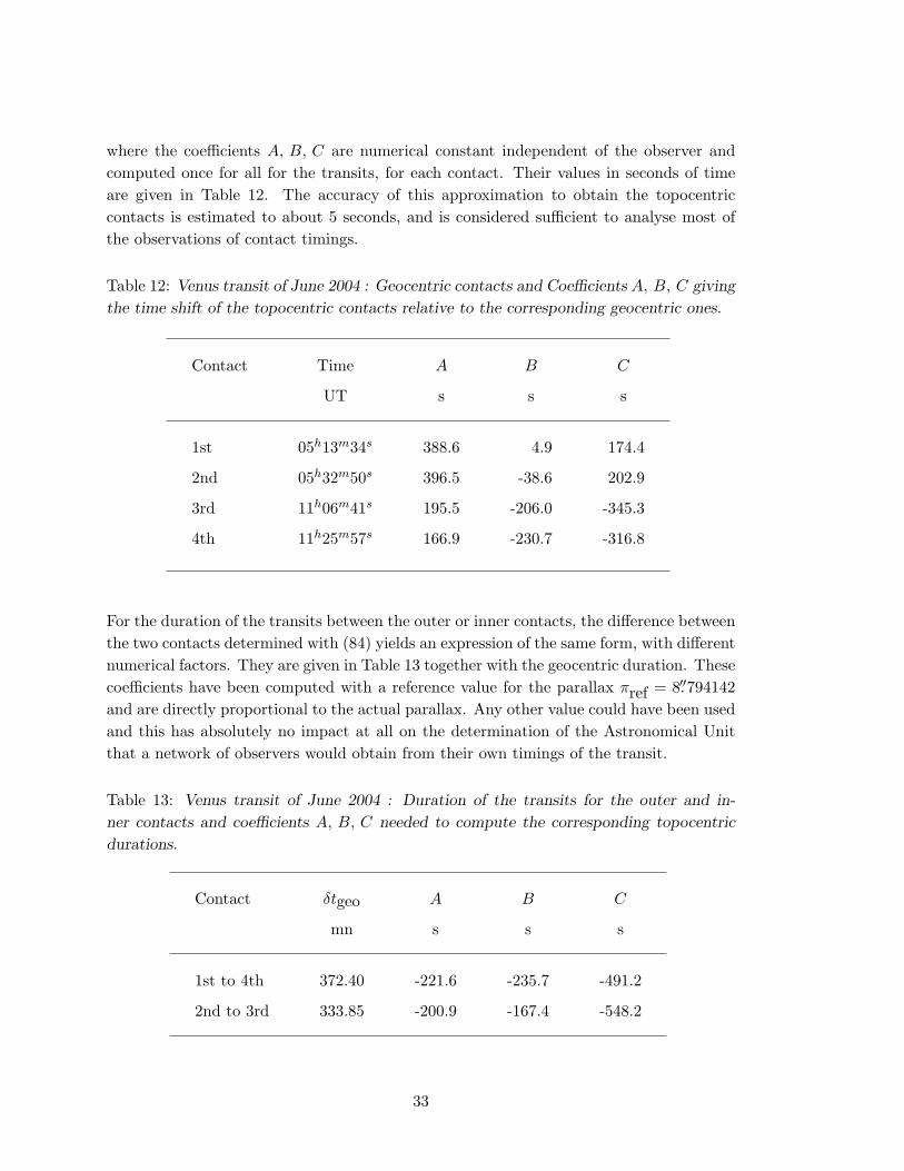
where the coefficients A, B, C are numerical constant independent of the observer andcomputed once for all for the transits, for each contact. Their values in seconds of timeare given in Table 12. The accuracy of this approximation to obtain the topocentriccontacts is estimated to about 5 seconds, and is considered sufficient to analyse most ofthe observations of contact timings.
Table 12: Venus transit of June 2004 : Geocentric contacts and Coefficients A, B, C giving
the time shift of the topocentric contacts relative to the corresponding geocentric ones.
Contact Time A B C
UT s s s
1st 05h13m34s 388.6 4.9 174.4
2nd 05h32m50s 396.5 -38.6 202.9
3rd 11h06m41s 195.5 -206.0 -345.3
4th 11h25m57s 166.9 -230.7 -316.8
For the duration of the transits between the outer or inner contacts, the difference betweenthe two contacts determined with (84) yields an expression of the same form, with differentnumerical factors. They are given in Table 13 together with the geocentric duration. Thesecoefficients have been computed with a reference value for the parallax πref = 8.′′794142and are directly proportional to the actual parallax. Any other value could have been usedand this has absolutely no impact at all on the determination of the Astronomical Unitthat a network of observers would obtain from their own timings of the transit.
Table 13: Venus transit of June 2004 : Duration of the transits for the outer and in-
ner contacts and coefficients A, B, C needed to compute the corresponding topocentric
durations.
Contact δtgeo A B C
mn s s s
1st to 4th 372.40 -221.6 -235.7 -491.2
2nd to 3rd 333.85 -200.9 -167.4 -548.2
33

Two observers measuring each at its location the duration of the transit between the twoinner contacts can determine the solar parallax from their measurements with (78)and(79), by computing the expected difference of duration of the transits between the twoplaces from the reference distance, and using the observed value in (79). A similar formulacan be written giving directly the astronomical unit in kilometres as,
1AU = 149.60× 10⁶ δtrefδtobs
(85)
As a numerical application consider an observer located at Nice ( O1 : λ = 7.◦30, φ = 43.◦72)and the second at Saint-Denis in the Island of Reunion (O2 : λ = 55.◦47, φ = −20.◦87). Onedetermines first the computed duration (between second and third contact) for each placewith (84), taking the coefficients A, B, C and the geocentric duration from the second lineof Table 13. One gets,
δt1 = δtgeo − 538.3 s = 324.87 mn (86)
δt2 = δtgeo − 40.0 s = 333.18 mn (87)
for the duration of the transit at Nice and at Saint-Denis. The differences in the durationbetween the geocentric event and the topocentric event expressed in seconds follow justfrom a straight application of (84) to the two locations. Therefore the theoretical differencebetween the two measurements computed with a reference astronomical unit of 149.60×10⁶
km should be,δtref = 498.3 s (88)
Assuming that the observed values for the duration are (with a reasonable random errorin the timing of about 20 s),
δt1 = 324.60 mn (89)
δt2 = 333.30 mn (90)
orδtobs = 522.0 s (91)
Therefore, they would find with (85) an astronomical unit of 142.9× 10⁶ km, or an errorof ∼ 5%.
It happens that the linear formula performs poorly in the middle of the Indian Ocean (seeFig. 7-bottom) and that in this particular case, a processing with the quadratic expressionwould be more appropriate. Essentially, one has to correct the observed duration for themagnitude of the second order terms before applying the result to the determination ofthe parallax with the linear terms.
34

ANNEX
Numerical data for the transit of June 2012
The following tables are identical to Table 4-5-6, but for the transit of 2012 with anextrapolated value of TT − TU = 65.8s.
Table 14: Venus transit of 5-6 June 2012 – Geocentric contacts
Contact Time X Y X Y θ H�
UT ′′ ′′ ′′/h ′′/h ′′ deg
1st 22h09m44s 633.84 738.38 -232.58 -60.92 945.72 152.78
2nd 22h27m33s 564.83 720.31 -232.58 -60.92 945.72 157.23
3rd 04h31m45s -847.59 353.06 -232.78 -60.07 945.69 248.27
4th 04h49m34s -916.66 335.23 -232.78 -60.07 945.69 252.72
35

Table 15: Venus transit of 5-6 June 2012. Coefficients for the topocentric contacts : linear
formula.
Contact A+ δA B + δB C + δC Γ b l
s s s s deg deg
1st -222.7 176.1 -277.3 396.9 -44.3 141.7
2nd -213.9 184.4 -296.9 409.8 -46.4 139.2
3rd 373.9 82.0 144.5 409.1 20.7 12.3
4th 371.4 59.0 125.0 396.3 18.4 9.0
2nd to 3rd 587.8 -102.5 441.4 742.2 36.5 350.1
1st to 4th 594.1 -117.1 402.2 727.0 33.6 348.9
Table 16: Venus transit of 5-6 June 2012. Coefficients for the topocentric contacts : second
order terms.
Contact C00 C22 S22 C21 S21 C20
s s s s s s
1st 2.2 -1.1 -0.0 -0.4 0.1 3.0
2nd 2.6 -1.1 0.1 -0.2 0.2 3.6
3rd -2.6 0.7 -1.4 -1.4 -0.2 -3.6
4th -2.2 0.5 -1.4 -1.2 -0.0 -3.0
2nd to 3rd -5.1 1.7 -1.5 -1.2 -0.4 -7.1
1st to 4th -4.4 1.6 -1.4 -0.8 -0.1 -6.1
36

Figure 9: Difference in seconds between the geocentric and topocentric time of the second(top) and third contact (middle), and difference of duration of the transit (bottom) for anypoint on the Earth (irrespective of the visibility)
37