the solar-b mission final report of the science definition ... · final report of the science...
TRANSCRIPT
/
NASA-CR-20462871
THE SOLAR-B MISSION
FINAL REPORT
of the
SCIENCE DEFINITION TEAM
Spiro Antiochos, Naval Research Laboratory, Chair
Loren Acton, Montana State University
Richard Canfield, Montana State University
Joseph Davila, Goddard Space Flight Center
John Davis, Marshall Space Flight Center
Kenneth Dere, Naval Research Laboratory
George Doschek, Naval Research Laboratory
Leon Golub, Harvard-Smithsonian Center for Astrophysics
John Harvey, National Solar Observatory, NOAO
David Hathaway, Marshall Space Flight Center
Hugh Hudson, Solar Physics Research Corporation
Ronald Moore, Marshall Space Flight Center
Bruce Lites, High Altitude Observatory, NCAR
David Rust, Applied Physics Laboratory, JHU
Keith Strong, Lockheed-Martin Solar & Astrophyics Laboratory
Alan Title, Lockheed-Martin Solar _z Astrophyics Laboratory
June 9, 1997
https://ntrs.nasa.gov/search.jsp?R=19970019636 2018-07-16T11:25:57+00:00Z

Contents
1 INTRODUCTION 1
2 SCIENTIFIC OBJECTIVES 2
2.1 Magnetic Field Generation and Transport ............... 2
2.2 Magnetic Modulation of the Sun's Luminosity ............. 9
2.3 Structure and Heating of the Chromosphere and Corona ....... 12
2.4 Eruptive Events and Flares ....................... 21
3 SOLAR-B INSTRUMENTATION 30
3.1 Optical Telescope and Magnetographs 1 ................. 30
3.1.1 Optical Telescope System 1 ................... 39
3.1.2 Filter Vector Magnetograph and Imager ............ 42
3.1.3 Spectro-Polarimeter ........................ 44
3.2 X-Ray Telescope ............................. 53
3.3 EUV Imaging Spectrometer ....................... 56
APPENDICES
A
62
The Solar-B Spacecraft 62
A.1 Orbit .................................... 62
A.2 Satellite Structure ............................. 62
A.3 Attitude Control ............................. 65
A.4 Data Storage and Transmission ..................... 67
B Projected Cost 68

1 INTRODUCTION
Solar variability is due to the energy that is generated deep in the Sun's interior by
nuclear burning, carried to the surface by convective motions, and finally transported
to the outer atmosphere and heliosphere by the Sun's magnetic field. This variable
transport of energy is the origin of all the many manifestations of solar activity that
drive the Sun-Earth connection. Magnetic fields play the central role in the variable
transport of the Sun's energy. The solar magnetic field modulates the thermal energy
that escapes the Sun's surface, the photosphere, in the form of black-body radiation,
and the magnetic field carries directly the non-thermal energy that produces the
dynamic corona and heliosphere. Variability in the Sun's nonthermal emissions drive
space weather and variability in the thermal radiation is an important driver of global
change.Our view of solar variability has been revolutionized by Yohkoh, an ISAS mission
with major NASA participation. Yohkoh has shown that the hot corona is extremely
dynamic, with magnetic reconnection, rapid heating and mass acceleration being
common phenomena. SOHO a joint ESA/NASA mission is now showing in detail
the physical parameters of plasma heating and acceleration. The next vital step is
to understand the magnetic origins of variability. Solar-B, the next ISAS mission, is
designed to address this fundamental question of how magnetic fields interact with
plasma to produce solar variability. Measuring the properties of the Sun's magnetic
field is the fundamental observational goal of Solar-B.
The mission has a number of unique capabilities that will enable us to answer the
outstanding questions on solar magnetism. First, by escaping atmospheric seeing, it
will deliver continuous observations of the solar surface with unprecedented spatial
resolution. Solar-B will allow us for the first time to observe the dynamics of the
elemental, discrete magnetic flux tubes that form the photospheric magnetic field. It
is the dynamics of these flux tubes that is thought to be responsible for the activity
observed in the corona by Yohkoh.
Second, Solar-B will deliver the first accurate measurements of all three compo-
nents of the photospheric magnetic field. In order to have the free energy necessary
to power solar activity, the magnetic field must contain electric currents. It is vital,
therefore, that all components of the field be observed so that the currents can be
calculated. However, the magnetic components transverse to the line of sight are
difficult to observe, and cannot be measured with any degree of accuracy if the field
is not spatially resolved. By resolving the magnetic structures, Solar-B will yield
measurements of the transverse field that will be truly revolutionary.
Finally, Solar-B will measure both the magnetic energy driving at the high-beta
photosphere and, simultaneously, its effects in the low beta corona. The mission
consists of a complement of instruments that will observe the solar surface and atmo-

sphereasonecoupledsystem. This instrument complementcontainsan optical vectormagnetograph for the photosphereand coordinated X-ray/XUV imaging telescopesand spectrographsfor the corona. As in Yohkoh,the US would havefull participationin all instruments and all the data. The US would contribute only one-quarter thecost of the mission; therefore, wewould be able to obtain facility classsciencefor aMIDEX price.
In addition to the many science rewards, Solar-B offers unique programmatic
opportunities to NASA. It will allow us to continue our cooperation in space science
with our most reliable international partner. Solar-B will deliver images and data
that will have strong public outreach potential. The science of Solar-B is clearly
related to the themes of origins and plasma astrophysics, and contributes directly to
the national space weather and global change programs.
2 SCIENTIFIC OBJECTIVES
The overarching goal for the Solar-B mission is to comprehensively understand the
solar photosphere and corona, as a system. To address this broad goal we identify
four promising areas of exploration:
* Magnetic field generation and transport
. Magnetic modulation of the Sun's luminosity
• Heating and structuring of the chromosphere and corona
• Eruptive events and flares
Taken together, these topics encompass much of the effort by the US and inter-
national solar physics communities, and are at the heart of solar variability.
2.1 Magnetic Field Generation and Transport
Generation of magnetic flux is believed to take place through the interaction of solar
rotation with the convecting, highly conductive plasma deep within the Sun. Once
generated, magnetic flux rises through the convection zone to the visible solar surface.
Recent results show that the topology of the magnetic fields, as they emerge into the
visible atmosphere, reflects the workings of both the dynamo and the passage through
the convection zone. The processes by which solar flux reconnects, erupts, and leaves
the Sun to produce a solar cycle are unknown. Solar-B will observe the topolog-
ical changes associated with magnetic flux emergence, reconnection, and eruption,
through simultaneous X-ray and vector magnetic field observations.
Challenges of Solar MagnetismUnderstandingthe generationof magneticfields, their emergenceinto the solarat-
mosphere,and their energeticconsequencesarechallengingand fascinating problemsin their own right. Not only doesthe study of the physicsof the solar plasma haveimportance for understandinghow the Sun influencesthe Earth and its space enviro-
ment, it also provides a cornerstone for understanding magnetized plasmas occurring
in other astronomical contexts.
Three aspects of solar magnetism have highest priority for Solar-B:
• The dynamo process within the Sun which is the origin of the solar magnetic
cycle.
• The processes which govern the transport and subsurface evolution of magnetic
fields as they rise to and penetrate the surface.
• The dispersal, decay, and ejection of magnetic energy and flux once the fields
have emerged.
To address these challenges, the key strength of Solar-B is its capability to simul-
taneously observe coronal structure and photospheric vector magnetic field.
The Solar Dynamo
Magnetic fields of lower main-sequence stars such as the Sun are believed to arise
from a dynamo process operating near the base of their convective envelopes. The
magnetic field is generated through the interaction of solar rotation with the con-
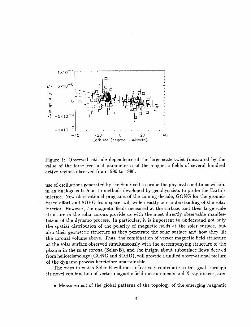
vecting, highly electrically conductive plasma. Evidence of this process" is seen in
the hemispheric dependence of the twist of active region magnetic fields (Figure 1),
which recent studies have shown cannot simply be explained in terms of differential
rotation or the dynamics of flux ropes rising through the convection zone. It is there-
fore believed that twisting of the magnetic field into flux ropes by subsurface flows is
a principal physical action of the dynamo process. This twist of the magnetic field
B = V × A, where A is the vector potential, contributes to the magnetic helicity
= f A • B dV, a topological quantity of both theoretical and observational interest.
This process is understood only in broad outline, as the best extant models of the
solar and stellar dynamos lack the ability to predict fundamental observed proper-
ties of the solar magnetic cycle. New observational inputs are now possible, through
vector magnetic field observations from space, which will enable advancement in this
important area. A major goal of Solar-B is to strengthen our understanding of the
solar dynamo.
To date we have only very limited knowledge of plasma motions and magnetic
fields deep within the Sun where the dynamo is believed to operate, but our knowl-
edge is rapidly improving as a result of recent developments in helioseismology: the
3
lx10 -7
,..-..., 5x10 -8
'E
0ID
0L_
_5xlO -8
-7-lx10
-40
I I I ,
-20 0 20
Lotitude (degree, +=North)
4O
Figure 1: Observed latitude dependence of the large-scale twist (measured by the
value of the force-free field parameter a of the magnetic fields of several hundred
active regions observed from 1990 to 1996.
use of oscillations generated by the Sun itself to probe the physical conditions within,
in an analogous fashion to methods developed by geophysicists to probe the Earth's
interior. New observational programs of the coming decade, GONG for the ground-
based effort and SOHO from space, will widen vastly our understanding of the solar
interior. However, the magnetic fields measured at the surface, and their large-scale
structure in the solar corona provide us with the most directly observable manifes-
tation of the dynamo process. In particular, it is important to understand not only
the spatial distribution of the polarity of magnetic fields at the solar surface, but
also their geometric structure as they penetrate the solar surface and how they fill
the coronal volume above. Thus, the combination of vector magnetic field structure
at the solar surface observed simultaneously with the accompanying structure of the
plasma in the solar corona (Solar-B), and the insight about subsurface flows derived
from helioseismology (GONG and SOHO), will provide a unified observational picture
of the dynamo process heretofore unattainable.
The ways in which Solar-B will most effectively contribute to this goal, through
its novel combination of vector magnetic field measurements and X-ray images, are:
• Measurement of the global patterns of the topology of the emerging magnetic
4

field (handednessand density of twist),
Measurementof the distribution of sizescales for the twist of the magnetic field,
an observable quantity fundamental to the dynamo process,
Observational description of the modes of evolution and expulsion of magnetic
flux and helicity from the Sun in relation to flux emergence, dispersal, and
reconnection.
Observational characterization of the role of reconnection and expansion of the
flux into the corona on the fields below.
Quantification, for the first time, of the flux history of individual solar active
regions, through measurements of the vector magnetic field as an active region
rotates across the solar disk.
Subsurface Transport and Flux Emergence
The evolution of magnetic flux as it is transported from its dynamo origin at
the base of the convection zone, upward through the convecting and rotating solar
envelope is surely geometrically complex. However, large-scale magnetic features such
as prominences, active region complexes, and coronal holes (as well as overall active-
region magnetic field twist, see Figure 1) suggest that the fields retain some of their
twisted topology in spite of their journey through the turbulent envelope of the Sun
(sinuous structures in Figure 2). Furthermore, recent theoretical work has indicated
that it may not be possible for the Sun to transfer large-scale helicity to smaller and
smaller scales, so that the solar magnetic field retains its large-scale helicity even after
it penetrates the surface.SOHO observations of the emergence of magnetic fields at the smallest scales yet
observed show that the process is a complex one. As well, it is a continuous one, in
which new flux emerges in the form of very small bipoles (ephemeral regions). Each
bipole, on average, bring to the surface a total flux of about 1019 Mx. These bipoles
bring enough flux to the surface to replace all of the magnetic field on the Sun ona time scale of 20 to 100 hours. The total field in the quiet Sun is 10 to 100 times
more than the net flux. The observed distribution of flux concentrations, the number
of a given flux versus flux at the SOHO resolution, can be predicted on the basisof a statistical mechanical model based on the assumptions that fields moving along
intergranular boundaries have a given probability of merging and canceling, and that
they spontaneously fragment in proportion to the amount of flux in the concentra-
tion. The merging, cancellation, and fragmentation rates have been measured and it
has been possible to predict the flux distributions of both polarities in very quiet Sun
and dense plage. When the flux concentrations observered at SOHO resolution are

Figure 2: Examples of the structuring of the X-ray corona bv the magnetic field,illustrated by selectedimagesfrom Yohkoh. A) helmet type streamer; B) arcadeofloops seenend-on; C) dynamic eruptive ejection with twist; D) flaring loops, loop-top heating; E) wishbone-shapedloops with cusps,one with heating concentrationin the cusp;F) loops; and G) S-shapedstructures betweenactive regions. (CourtesyLockheed Martin Solar & Astrophysics Group.)
6

OBSERVATION:
THEORY:
Figure 3: Theoretical toroidal flux-rope model of the magnetic field of a "Delta"
spot, based on observations from the ground-based Advanced Stokes Polarimeter
(center) and Yohkoh (left). The ASP vector magnetic field maps show the concave
upward nature of the vector field present in the small "delta" sunspot at the left.
The corresponding narrow-band chromospheric image in Ha shows the presence of
a prominence "filament" forming directly above the line separating fields of opposite
magnetic polarity. The theoretical model of the 3-dimensional magnetic field geom-
etry appearing at the lower right shares many features common to both the vector
fields observed at the photosphere and the twisted nature of the field lines in the
corona as inferred from the X-ray images. Some field lines in the theoretical model
appear to bridge the opposite polarities along straightforward paths. Others take
more circuitous paths which experience one or more local minima above the photo-
sphere. The minima of some such field lines are shown, suggestive of cool prominence
material residing stably in the corona, isolated from the high temperature corona by
the magnetic field.
7

examined at higher resolution with groundbased magnetograms, the concentrations
are observed to break up into smaller fragments that are embedded in the intergran-
ular lane pattern just as the concentrations at the MDI resolution are embedded in
the supergranular pattern.
A new generation of instrument capable of providing vector magnetic field mea-
surements is needed to quantitatively describe the state of the magnetic field as it
emerges. The magnetic field is a vector quantity, and it is not sufficient to measure
only one component of this vector to answer the questions we pose. This information
is crucial not only to understanding the large-scale evolution of the field which con-
cern the dynamo process, but also the topology of structures of the outer atmosphere
of the Sun, as shown dramatically in Figure 3. Several important questions regarding
subsurface flux transport and emergence may be addressed by Solar-B:
Does the natural buoyancy of magnetized plasmas drive the emergence of mag-
netic flux, or are the inductive effects of flows such as differential solar rotation,
meridional, supergranular, and granular flows important, as well?
• What is the magnetic flux history of individual solar active regions, during the
process of flux emergence? Does flux submergence play a significant role?
Does submergence of magnetic fields commonly occur, presumably as a result
of magnetic tension forces in curved subsurface magnetic fields, or is this phe-
nomenon rare due to both buoyancy and the rapid expansion of field structures
into the corona?
Dispersal, Decay, and Ejection of Magnetic Fields
The processes by which the magnetic flux of solar active regions disappears from
the solar surface remain largely unknown, yet we know such processes must exist
because the net polarity of the magnetic field in each hemisphere reverses with each
22-year magnetic cycle. It is suspected that sunspot magnetic fields are dispersed,
through the action of turbulent convection, into the quiet Sun in the form of many very
small, intense magnetic flux tubes, which comprise the magnetic network of the quiet
Sun. Their fate from that point on is even more speculative, but either they undergo
reconnection and dissipation in the form of micro-flares and atmospheric heating, or
they are ejected into the corona and solar wind. As yet, these speculations have
been neither refuted nor supported because we lack the high resolution, continuous
observations of the photospheric magnetic field which Solar-B will provide.
In order for the solar magnetic polarity to reverse itself every 11 years, it is proba-
bly necessary for the Sun to expel the large-scale twisted field structures, in the form
of coronal mass ejections. There is no other obvious avenue for the Sun to dissipate
the large-scale helicity which clearly appears to be present in solar magnetic fields in

the form of the long chromospheric filaments which commonly reside at high latitudes.
Interestingly, the extremely high resolution magnetic observations from Solar-B are
absolutely necessary to define the nature of even the largest scale structures of the
solar magnetic field and its resulting coronal structure.The most important objectives of Solar-B magnetic field measurements for eluci-
dating the processes by which magnetic flux evolves are:
• To identify the modes of decay and dispersal of active regions in quantitative
terms, allowing for the contributions to the flux loss by reconnection, ejection,
and dissipation into the quiet magnetic network,
• To explore the physical properties of the intense, but very small magnetic flux
tubes which apparently are responsible for most of the l 1-year periodic vari-
ability of the net radiative output of the Sun,
• To determine the fate of quiet region magnetic flux by in-situ dissipation of the
accompanying electric currents (leading to atmospheric heating, either impulsive
or steady), by reconnection (leading to small scale ejection of magnetic flux - a
process not yet observed but within the capability of Solar-B instruments), or
even by submergence, and
• To determine the nature and importance of turbulent, weak internetwork mag-
netic fields in the context of the apparently dominant intense fields.
Whenever quantitative magnetic flux measurements are called for, as in the objec-
tives stated above, measurement precision is essential. Solar-B will provide the first
opportunity to explore vector magnetic fields with sufficient precision and temporal
continuity to address these fundamental objectives.
2.2 Magnetic Modulation of the Sun's Luminosity
The Sun is known to vary on many time scales. On short time scales, it varies in
its total luminosity due to both the global p-modes and due to granular convection
in a nearly random fashion with characteristic times of a few minutes, and with
an amplitude of a few times 10 -s. The quasi-periodic solar luminosity variability
at longer periods is roughly a hundred times greater in amplitude. Time scales for
these components of the solar luminosity spectrum range from the shortest observable
times associated with solar flares and other dynamical events, through the daily and
monthly evolutionary times of active regions, to the decadal time scales of the solar
cycle, and even to time scales of centuries associated with long-term variations of
solar activity. The underlying cause of this dominant component of solar variability
is the Sun'smagnetic field. Variable solarmagneticactivity is therefore the dominantsourceof all those fluctuations in the solar output deemedimportant to the Earthand its spaceenvironment.
Understanding the magneticorigin of this variability - the generationof the mag-netic fields, their emergenceinto the solar atmosphere,and their energetic conse-quences- is a challengingand fascinating problem, discussedabove. Ultimately, theprediction of solar variability at all wavelengthswill most likely hingeon afirm physi-cal understandingof the solarprocessesinvolved. Solar-B is a missionwhich is poisedto makeunprecedentedadvancesin our understandingof solar magnetismasa globalprocess,and specificadvancestoward understandingthe magnitude and causeof solarluminosity and spectral irradiance variations, asoutlined below.
Accounting for Sources of Solar Luminosity Variations
That the solar luminosity varies with the 11-year solar activity cycle at the level of
0.1 - 0.2% has been clearly demonstrated by several space-borne experiments during
the last 17 years. Short-term dips in the luminosity at times of high activity are due
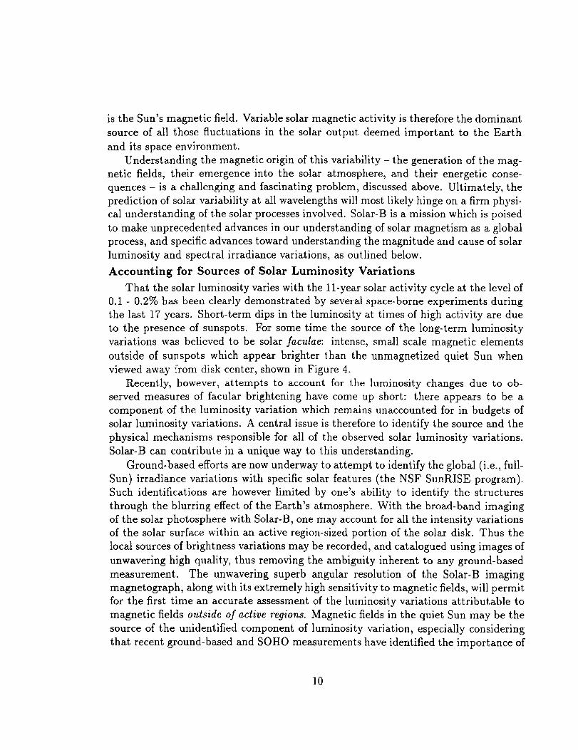
to the presence of sunspots. For some time the source of the long-term luminosity
variations was believed to be solar faculae: intense, small scale magnetic elements
outside of sunspots which appear brighter than the unmagnetized quiet Sun when
viewed away from disk center, shown in Figure 4.
Recently, however, attempts to account for the luminosity changes due to ob-
served measures of facular brightening have come up short: there appears to be a
component of the luminosity variation which remains unaccounted for in budgets of
solar luminosity variations. A central issue is therefore to identify the source and the
physical mechanisms responsible for all of the observed solar luminosity variations.
Solar-B can contribute in a unique way to this understanding.
Ground-based efforts are now underway to attempt to identify the global (i.e., full-
Sun) irradiance variations with specific solar features (the NSF SunRISE program).
Such identifications are however limited by one's ability to identify the structures
through the blurring effect of the Earth's atmosphere. With the broad-band imaging
of the solar photosphere with Solar-B, one may account for all the intensity variations
of the solar surface within an active region-sized portion of the solar disk. Thus the
local sources of brightness variations may be recorded, and catalogued using images of
unwavering high quality, thus removing the ambiguity inherent to any ground-based
measurement. The unwavering superb angular resolution of the Solar-B imaging
magnetograph, along with its extremely high sensitivity to magnetic fields, will permit
for the first time an accurate assessment of the luminosity variations attributable to
magnetic fields outside of active regions. Magnetic fields in the quiet Sun may be the
source of the unidentified component of luminosity variation, especially considering
that recent ground-based and SOHO measurements have identified the importance of
10

Max Min Max
_.200 _ unspot um erJ.2
. _ Irradiance Increase "_
loo. o.10 0.078 80 82 874-86-88 90 92 94
Years
Figure 4: Visible continuum image of the bright faculae in and around a sunspot
group. The supergranular cell/network pattern is seen in the outskirts of this re-
gion. The spatial resolution is about a quarter of an arcsecond, enough to show the
photospheric granulation quite well. Each bright facular element marks a magnetic
flux fragment. The magnetic and flow fields in each fragment somehow result in the
enhanced photospheric emission, which when summed over all faculae accounts for
much of the rise and fall of the the solar luminosity with the sunspot cycle. Because of
blurring by turbulence in the Earth's atmosphere, even at the best sites ground-based
observatories obtain only rare glimpses of the Sun at this resolution (0.25 arcsecond).
Because of the perfect seeing in space, the 50 cm telescope on Solar-B will provide
continuous viewing of the photosphere and chromosphere at this resolution. (G-band
image from the 50 cm Swedish Vacuum Telescope on La Palma.)
11
the non-active region fields. With Solar-B, detailed studies of the root causes of solar
luminosity variations may be carried out during the rapidly changing declining phase
of the solar activity cycle. It may be possible to determine trends in the relative
contributions of active region and quiet region magnetic fields to the observed global
luminosity variations.
Solar-B will provide the first capability for precision diagnostics of the evolution of
solar magnetic features at high angular resolution. This will enable one to investigate
in detail the underlying radiative and magnetohydrodyamic processes governing these
structures, and thus enable us to understand the physical basis for the solar luminosity
variations. With Solar-B's breakthrough to steadfast subgranular spatial resolution,
we will be able to answer the following questions:
• How do the brightness and lifetime of a facular element depend on the strength,
total flux, and inclination of the magnetic field in the element?
• How is the magnetic field that forms a facular element assembled by the granular
flow and how is it dispersed in the demise of the facular element?
• Are facular elements predominantly unipolar, or do they occur preferentially
between colliding magnetic field clumps of opposite polarity?
Spectral Irradiance Variations
The solar radiative output is increasingly more variable as the wavelength of the
emitted radiation decreases. Such variations have a major influence on the Earth's
upper atmosphere, and as a result, may also influence climate variations. Just as with
the luminosity variations, nearly all of the irradiance variations at short wavelength
may be traced directly to the injection of magnetic fields into the solar atmosphere.
Besides being an important driver of the space environment of the Earth, the mag-
netic heating and dynamics of the outer solar atmosphere presents us with the best
opportunity to understand the physics of related processes common to a wide range
of other astrophysical systems. The power of Solar-B to address these fundamental
questions surrounding the heating and structuring of the outer solar atmosphere is
the topic of the following section.
2.3 Structure and Heating of the Chromosphere and Corona
The forces that dominate in the dense photosphere differ substantially from those
which dominate in the upper layers of the solar atmosphere. For the most part,
hydrodynamic forces dominate in the photosphere, and only within the strongest
magnetic field structures, such as sunspot umbrae, do magnetic forces rival the hy-
drodynamic forces. However, the density of the solar plasma falls off very rapidly
12

with height due to the extremely small scaleheight low in the solar atmosphere,sothat in the higher layers of the atmospherethe magnetic field often dominates itsdynamics and structure. The structure imparted by the magnetic field gives rise tothe phenomenawe observein these structures, and it also strongly affects physical
processes leading to heating of the atmosphere. Thus, understanding the nature of
the various phenomenological structures we observe in the solar atmosphere will pro-
vide important links toward understanding the nature of the heating of the outer
atmospheres of stars.
Chromosphere
In the chromosphere a complex arrangement of magnetically-dominated and rel-
atively field-free regions is observed. It appears that in non-magnetic chromospheric
regions, acoustic heating is likely to be the dominant energization process. Photo-
spheric convective motions generate sound waves which may steepen into shock waves
that dissipate to heat the field free regions of the chromosphere, such as in the cen-
ters of supergranule cells. The emission from magnetic regions of the chromosphere
is well known to be in excess of that in non-magnetic regions; hence, some additional
heating must occur due to the presence of the magnetic field. The enhanced chromo-
spheric heating in the magnetic network could be due to the turbulent motions of the
upper convection zone which generate MHD waves that travel outward in the flux
tubes. Dissipation of this wave energy could give rise to the enhanced chromospheric
emission seen in the magnetic lanes of the network.
Solar-B will enable us to follow the shocks and their heating with height in the
chromosphere and transition region by observing appropriate EUV lines through
imaging spectroscopy (see Figures 5 & 6) with high spatial, temporal and spectral
resolution. With its vector magnetograms of high spatial resolution, Solar-B will
easily be able to distinguish the magnetic field at the boundaries of the supergran-
ular cells from their relatively non-magnetic interiors. Simultaneous observations of
the magnetic field and of longitudinal and transverse motions will help us gauge the
nature and magnitude of the generation, propagation and dissipation of these waves
that could provide most of the heating of the hottest part of the solar chromosphere.
Interesting questions which we can address with this unique combination of Solar-B
observing capabilities include:
• Are non-magnetic regions of the chromosphere heated by shocks?
• How are magnetic regions of the chromosphere heated, and why are they so
different from the field free regions?
• How is convective energy transferred from the photosphere to the corona?
13

2000 -
500"
50O I[XX)
orc$1_c
1500 2000
50O 1 O00 15 O0
count =/line/arcse¢ 2/_
FuII Disk In Carbon HI
Instrument: SUWERUne: C III
Ternperc!.ure: 70 000 K
Raster Step: 1.14 orcsec
2000 2500
28Jan.96
Observatory:, SOHO
Wovelength: 977,02Slit 2:1.0 * 300 ar_ec =
Exposure "13me: 7 s
Figure 5: A full disk image showing the structure of the chromosphere in CIII
built up from a series of slit spectrograph images. (Image provided courtesy of the
SOHO/SUMER instrument team. SOHO is a cooperative mission between ESA and
NASA).
14

Figure 6: Explosiveeventsobservedby SUMER on28March 1996in the emissionlineof Si IV at 1393A, formed in the transition regionat about 100,000K. The pictureshowsa time seriesof 60 Si IV spectra,eachwith an exposuretime of 10s, coveringa time interval of 10minutes altogether. The spectral window is 25 pixels, allowingobservationsof redshifts (to the left) and blueshifts (to the right) up to approx. 100km/s. The north-south extensionof the slit coversapprox. 84.000km on the Sun (120arcsec). (Imageprovided courtesyof the SOHO/SUMER instrument team. SOHO isa cooperativemissionbetweenESA and NASA).
15

Corona
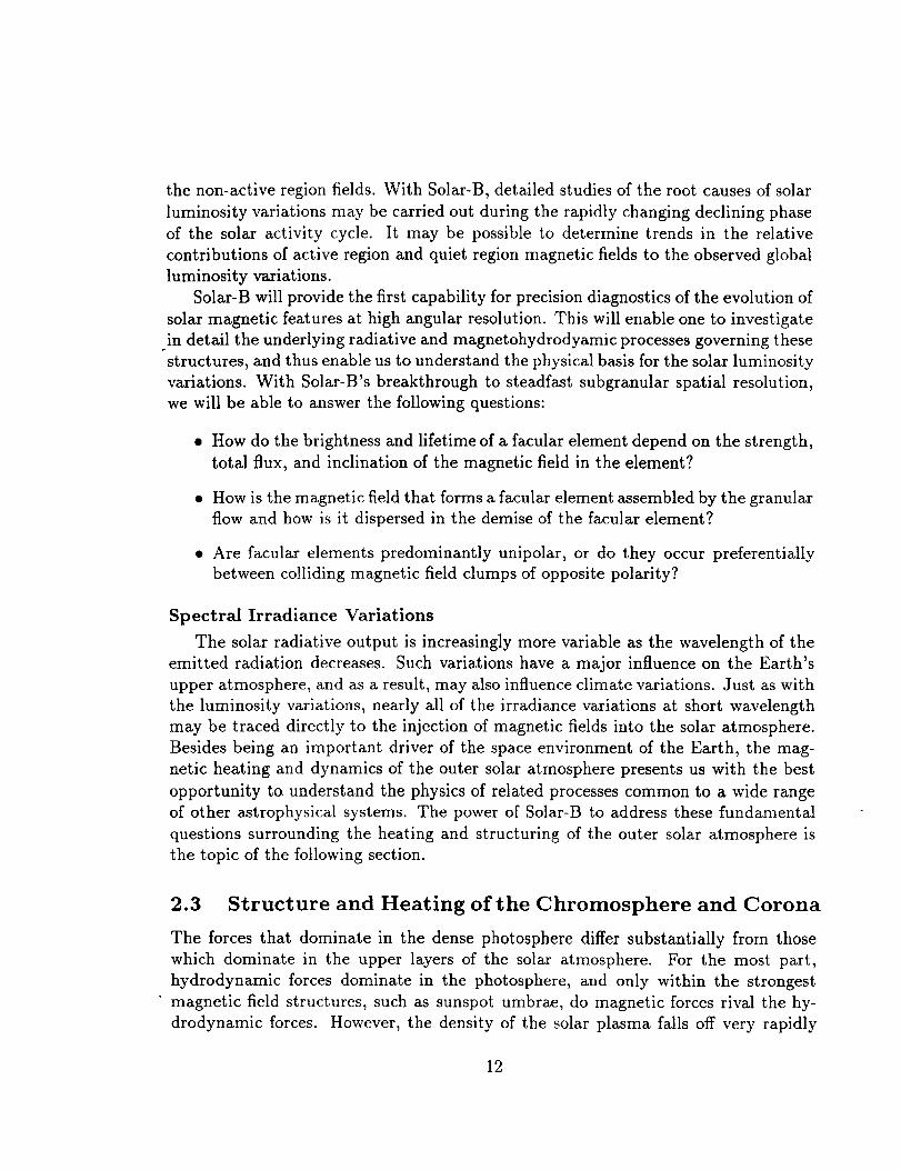
Itiswellknown from ¥ohkoh and EIT images that coronal emission ishighly struc-
tured (seeFigure 7). A number of recent studieshave emphasized the importance of
thermally differentiated imaging as part of the program to understand the heating and
structuring of the solar corona. It has long been known that very different structures
are seen in ground-based eclipse data in, e.g., the 'red line' (Fe X) compared with the
'green line' (Fe XIV). In soft X-ray observations, this point has been summarized by
noting that the observed coronal loop structures may be viewed as relatively isolated
mini-atmospheres, each with its own temperature and density structure. Because of
the marked difference in observed coronal parameters within small spatial distances,
it appears that the coronal heating mechanism can have markedly different effective-
ness in portions of the atmosphere which are otherwise indistinguishable. This idea
was made evident by observations such as the simultaneous NIXT and Yohkoh SXT
comparison which were carried out in April 1993.
Although the overall appearance of an active region observed in the two pass bands
is the same, close examination indicates that substantially different structures are seen
at 2.5 x 10⁶ K in the NIXT vs. 4 x 10⁶ K in the SXT. The comparison shows that
there are clusters of loops seen in one temperature range which are entirely invisible in
the othe:: this effect works in both directions, so that both instruments fail to detect
structures which are present in the corona and which must be presumed to play a role
in coronal dynamics. The conclusion from this work is that instrumentation which
detects an entire series of successive ionization stages of the same element is needed,
in order to not "miss" any of the emitting material.
It is generally agreed that the heating of the corona and chromosphere is driven
by convective motions in the photosphere, and that the transfer of energy is somehow
mediated by the magnetic field.
Two broad classes of theories have been developed to explain how the kinetic
energy of convection is thermalized in the corona. (1) Rapidly fluctuating motions
may produce MHD waves which propagate into the corona where they are resonantly
absorbed. The wave theory is able to reproduce the coronal structuring and the
necessary heating rate, however unambiguous evidence for sufficient wave power in
the corona has never been obtained. (2) The second broad class of heating mechanism
suggests that the corona may be heated by the dissipation of electric currents. These
currents are generated by the slow, shuffling motions of the magnetic flux bundles in
the photosphere, and the subsequent twisting and braiding of the coronal magnetic
field. In the corona these currents are resistively dissipated in thin current sheets.
As new magnetic flux erupts from below the photosphere, previously emerged flux
must be dissipated or ejected into the solar wind to maintain a steady state. Recon-
nection is a process by which the free energy contained in non-potential magnetic
fields (or, equivalently, contained in the electric currents which support them) may
16
51 "Xll 52041 A Fe xlv 333,78 a C_ x 557,68 A
Fe Xlll :34,B.18 A HI I 5e4.Z=O A Ire XIV _,5:LI_ A 355.04 A 51 X 356,,H- A
O HI 599.51 A Fi, XVI 360.79 1_ IX 36B,06 A 0 V 629.62 A
CDS NIS Raster, 6-Sep-1996 06:24:33LARGEBPZ -- Active Re91on on Limb -- s+Sg4.r00,flt_
Center = (1011",--334"), 51ze -- 244-'x240"
Figure 7: Images of a set of coronal loops as seen at the solar limb in emission
lines representing temperatures from 100,000 K to about 4 x 10⁶ K. Images were
constructed by rastering the slit. These images demonstrate the strong temperature
gradients present in the corona. (Image provided courtesy of the SOHO/SUMER
instrument team. SOHO is a cooperative mission between ESA and NASA).
17

SOHO views of polar plumes1996 March 7
Top to bottom:
MDI ki- ,r_, magnetogramEIT Fe IX/X 171 A imageEIT He II 304 A image
Figure 8: These images by the Extreme-ultraviolet Imaging Telescope (EIT) on board
SOHO show ultraviolet images of polar plumes near the south solar pole at about 1.5
million degrees Celsius in the Fe XII emission line at 195 A (top) and at somewhat
cooler temperature at about 1 million degrees in the Fe IX/X emission lines at 171 A
(bottom). These images represent the first opportunity scientists have had to see the
detailed development over time of the plume structures, at least at the solar poles.
(Image provided courtesy of the SOHO/MDI and EIT experiment teams. SOHO is
a cooperative mission of ESA and NASA).
18

Figure 9: Comparison of the X-ray corona of an active region with the roots of its
magnetic field in photosphere. The X-ray emission is brightest where coronal heating
is strongest, showing that in this active region the strongest heating was in the most
strongly stressed (most nonpotential) magnetic field. The left panel shows a vector
magnetogram of AR 6982 (from the NASA/MSFC solar observatory); the strength
of the line-of-sight component of the magnetic field is shown by the contours (solid
for positive polarity, dashed for negative polarity), the direction and strength of
the transverse component of the field are shown by the direction and length of the
distributed tic marks. The right panel shows a coronal X-ray image of this active
region (observed by Yohkoh) superposed on the line-of-sight field contours (white for
positive; black for negative).
19

be transformed rapidly into heating, massmotions, and/or structural changesof plas-mas, and it likely plays the dominant role in the continual readjustmentof the globalsolar field. The Yohkoh missionrepresentsa milestonein the observationof coronalmagnetic structures, and hasdemonstrated the large variety of magnetic topologieswhich canexist in the corona(Figure 2). It hasprovided particularly strong evidencefor magnetic reconnectionon a wide range of size scales. Solar-B, with its uniquecombination of crucial magnetic field measurementsin the photosphereand high res-olution observationsof the solarcorona,will be ideally poisedto addressthe followingimportant questions regarding the role of heating and reconnection in the magneticevolution of the solar atmosphere:
What processes lead to the open magnetic field structures which dominate the
mass flux of the solar wind, yet which apparently extend down to the base of
the corona?
• How does the magnetic field support and thermally insulate the cool condensa-
tions, such as prominences, embedded in the solar corona?
What are the relative roles of in-situ coronal reconnection and evolution of
the photospheric magnetic field for structuring of large-scale coronal magneticstructures?
The bulk of the hot coronal plasma is in the form of loops. Each loop is believed
to correspond to a magnetic flux tube. Motions at the foot points of magnetic loops
are believed to give rise to the heating which results in the X-ray emission of the
loop plasma. There are two major classes of proposed heating mechanism: (1) slow
motions shear the magnetic field and generate electrical currents which can heat the
atmosphere by ohmic dissipation, or result in localized impulsive heating by reconnec-
tion (e.g. microflares) and (2) rapid shaking of the flux tubes generates MHD waves
which when dissipated also could heat the coronal plasma. Both must be present to
some degree; however, which of these mechanisms is dominant? Figure 9 illustrates
the puzzle posed by observations having moderate spatial resolution. The transverse
field is highly sheared along part of the polarity inversion line. The right panel shows
a Yohkoh SXT image of the region, with selected longitudinal field strength contours
superposed. Although much of the enhanced heating is in obviously highly stressed
fields, some is not.
Another possibility for the heating of the magnetic regions of the chromosphere
is microflaring seated in the mid to low chromosphere. This would require a mixture
of opposite polarities on arcsecond to subarcsecond scales in the heated areas. The
microflaring might be the source of spicules and waves that in turn contribute to
the heating of the chromosphere and corona. A high-resolution vector magnetograph
2O

in space (such as envisionedfor Solar-B) will reveal whether or not the requisite
mixture of polarities is present, and whether the mixed-polarity fields contain enough
free energy (e.g. shear).
• Is the heating dominated by the dissipation of waves or electric currents?
• Is the heating mechanism different for active regions, the quiet Sun, and coronal
holes?
• What is the role of spicules and macrospicules in the transport of mass and
energy between the chromosphere and corona?
2.4 Eruptive Events and Flares
Some of the most fundamentally important effects that force changes in our local
space environment originate in eruptive events on the Sun. Solar eruptions range
over orders of magnitude in size, duration and energy output. Examples of such
events vary in size from spectacular flares and coronal mass ejections (CMEs), which
have direct and measurable effects on the Earth, to innumerable tiny spicules and
coronal jets, which may only impact the Earth indirectly - through their coronal
heating and subsequent solar wind generation. This leads us to the basic question:
• Are these highly diverse eruptive phenomena caused by the same fundamental
physical processes? If so, what are they?
Eruptive events can be very rapid. This requires, for the larger events at least,
that the energy be stored in the corona and released in a catastrophic manner. Hence,
we must understand:
• How is a critically unstable state produced by energy buildup?
• How is the eruption triggered?
• How does the eruption propagate?
To accomplish these ambitious goals we have to be able to probe the solar photo-
sphere with high spatial resolution to determine the evolution of the vector magnetic
field, which is an indicator of free energy buildup. In addition we need to determine
the topology, location and timing of the energy release. The determination of these
boundary conditions will require high-resolution and high-cadence coronal imaging.
To understand the physical and dynamic environment of the energy release process
to help constrain MHD models, we will also need coronal spectroscopy with high
21

LASCO C3 9-Ju1-1996 15:38 UT
Figure 10: Large coronal mass ejection (CME) observed by the LASCO C3 corona-
graph on SOHO. The size and location of the Sun are shown by the white circle in
the center of the shadow of the occulting disk.
spectral resolution. Solar-B will supply the broad new observational view needed for
this purpose.
The recent results from SOHO EIT show clearly that even at solar minimum the
Sun is almost continuously producing eruptive events over a wide range of spatial and
temporal scales. Solar-B will be launched during the declining phase of the current
cycle and therefore should see a full range of solar activity levels from intense flaring
to quiet solar-minimum conditions. Consequently, Solar-B will be an ideal tool to
investigate the evolution of the magnetic field that leads to plasma erupting from theSun.
The Buildup to an Eruption
Eruptions can happen rapidly (in seconds) so there is insufficient time to transport
energy from remote sources and have a mechanism capable of dissipating it efficiently
and quickly enough. Hence it is generally accepted that the energy is stored in
nonpotential (sheared) coronal fields prior to the event. But the question remains
as to how the fields become sheared. Possible explanations for the origin of these
magnetic stresses include:
• Footpoint motion caused by the convection flows visible in the photosphere;
22

\\\ !I_ /
Figure 11: Spicules. Top: side-view sketch of the clustering of spicules in the magnetic
network formed by supergranule convection cells. Bottom: high-resolution H-alpha
filtergram from Hida Observatory.
23

Figure 12: Characteristic magnetic shear at the site of an eruptive flare. The right
panel shows a Yohkoh soft X-ray image of an eruptive flare during its explosive phase
(the diffuse feature to the lower left is being formed by ejection of hot plasma from
the bright core region); the X-ray image is superposed on contours of the line-of-sight
component of the photospheric magnetic field (solid contours for positive polarity,
dashed contours for negative polarity); the bright core of the flare straddles a polarity
inversion line in a region on strong (,_ 1000 gauss) magnetic field. The left panel shows
a Mees Solar Observatory vector magnetogram with the same field of view as the right
panel; the bold dashes show the strength and direction of the transverse component
of the photospheric magnetic field (the strongest transverse field along the inversion
line under the flare is _ 1000 gauss); the line-of-sight field component is shown by the
same contours as in the upper panel (contour levels: 100, 200, 400, and 800 gauss).
The field along the inversion line is seen to be strongly sheared, relative to what one
would expect of a potential field.
24

• Proper motions of flux tubes in the photosphere due to the rotation or relative
motion of sunspots;
• The emergence of magnetic field stressed far below the photosphere, perhaps
by the solar dynamo itself.
The answer, of course, could be a combination of these physically different mech-
anisms.
Solar-B will be able to follow the build up of energy in the magnetic field because
of its unique vector magnetogram capability and its orbit. Such measurements are not
possible from the ground, at the high spatial resolution available to Solar-B, because
of the image distortion due to the Earth's atmosphere. Equally importantly, Solar-B
will have continuous coverage of the Sun because it is in a Sun-synchronous orbit. In
contrast ground based observatories can observe only 6-8 hours each day assuming
the best of conditions. The Solar-B view of the changing magnetic fields will produce
a revolution in our understanding of the emergence and dissipation of the strong solar
magnetic fields.
A question that has troubled solar observers for years concerns the existence of
coronal signatures prior to an eruption. Solar-B with its high cadence, continuous
coverage and the high spatial resolution of its coronal images and spectra should be
able to identify any coronal indicator of the build up of energy, e.g., an increasing
shear of the coronal loops with respect to the neutral line, changing energy dissipation
in the loops or increased dynamic activity (turbulence or flows). The identification
of such a signature could, for the first time, allow us to make reliable predictions of
solar eruptions, one of the primary goals of the space weather program.
Triggering Solar Eruptions
There are several possible mechanisms to expl_n the triggering of an eruptive flare
or coronal mass ejection. It can be driven by an essentially ideal process such as a kink
instability or a resistive instability (e.g., tearing). Yohkoh has already demonstrated
the importance of reconnection in the flare process by showing the dramatic evolutionof the coronal fields as the result of such events. While this can be accounted for by
the relaxation of the field after the event (i.e., after the explosive eruption of the
magnetic field) there is still the intriguing idea that reconnecting magnetic field may
also be the origin of the instability.
Solar-B can attack the problem of the triggering mechanism in a number of ways
using combinations of the vector magnetic field and coronal imaging data. For exam-
ple, the new observations can: ,,
• Locate the time and the site of the initiation of the energy release
25

Figure 13: Large eruptive flare on the limb; soft X-ray image from Yohkoh. Thisspiked-top flare arcadeis typical of flaresthat developin tandem with a coronalmassejection and are centeredin the stressedmagnetic field that explodes to drive theejection.
• Determine the critical state of the coronal and photospheric fields at the timethat the magneticconfiguration becomesunstableand erupts
• Determine at what stageof the event the coronal fields reconfigure
• Derive changesin the 3-D field configuration,including topology changes,through-out the event
• Determinephysical parametersin the eruptive and pre-eruptive plasma suchastemperature and turbulence
Transport Effects
The combination of Yohkoh and SOHO is proving to be a very powerful tool
in understanding the propagation of solar eruptions, particulaxly CMEs. However,
Solar- B will determine the vector magnetic field during these phenomena. It will
also bring much superior (continuous) coverage, plus higher spatial and temporal
resolution. Solar-B will definitively follow the changes in the magnetic configuration
of a region during an eruption. There is also the tantalizing prospect of seeing a
relaxation directly in the photospheric fields and consequently being able to derive a
self-consistent energy budget for such an event.
26

_ i ¸ °
Figure 14: Large coronal mass ejection observed by the SOHO LASCO C2 corona-
graph, and superposed simultaneous flare arcade observed by the Yohkoh SXT.
27

Figure 15: Solar X-ray jet and model. Right: X-ray jet observedby Yohkoh. Left:sketch of magnetic field configuration and reconnection inferred from observations.Top: 2-D MHD simulation.
28

agneUc reconnectlon point
Gas flow associated withmagnetic reconnectlon
elocity" 3000 km/s)
Shock wave front
#___Hard X-ray source
__. Accelerated •ff_ _b_electrons •
///_ Ir--_: _\\ % B_ht loopun"
l Itl \ Lc o.,os,h."o
Figure 16: Bright-topped flare images and model. Upper left: compact flare loop
observed end-on at limb by Yohkoh: hard X-ray contours superposed on soft X-ray
image. Lower right: flare arcade with bright cusp at top observed in soft X-rays by
Yohkoh. Lower left: 2-D reconnection picture that Solar-B observations and advanced
MHD modeling will test and extend to 3-D.
29

Theory and Modeling of Solar Eruptions
The study of eruptions that followed the discovery of coronal jets by the Yohkoh
team naturally led to attempts to understand the process theoretically, and to model
it numerically. The Solar-B data would equivalently revolutionize our view of eruptive
events by providing accurate boundary conditions and evolving physical parameters
to feed into the models. The 3-D magnetic field data are crucial for producing realistic
3-D simulations of the overall eruptive process. It is only when we can fully simulate
the observations in their entirety that we can claim to have answered the above
questions.
In the last decade there has been enormous progress in the development of 2-
D and 3-D numerical simulation capabilities due to the development of massively-
parallel computers coupled with the development of highly sophisticated numerical
techniques. The goal of the National High Performance Computing and Communi-
cations Program is to develop machines that by the turn of the century will be able
to operate at the teraflop rate. With these speeds it will be possible to perform fully
time-dependent simulations with grids of order 1024 a, so that we can finally achieve
closure between data and theory. Solar-B provides the high resolution observations
necessary to test and refine this next generation of numerical models.
3 SOLAR-B INSTRUMENTATION
The over-arching goal of Solar-B is comprehensive understanding of the solar pho-
tosphere and corona as a system. Our observational approach addresses this goal
through the use of optical and X-Ray/EUV telescopes. We have discussed four spe-
cific scientific goals above, and Table 1 links them to specific measurements and
instruments. In the strawman payload we describe here, the photospheric measure-
ments are made with a 50 cm aperture visible-light telescope, which is an integral part
of the spacecraft structure. This instrument includes both imaging and spectrograph
packages in its focal plane. The coronal measurements are made with an X-Ray/EUV
imager and an EUV imaging spectrograph.
3.1 Optical Telescope and Magnetographs 1
We propose to fly a ,-,50 cm diameter telescope with Solar-B, which would enable
us to perform high resolution and continuous observations of magnetic and velocity
fields, something we cannot achieve from ground. The focal plane package of the
telescope should consist of filter optics and spectrograph. Filters are used for high
time resolution observations, in which the narrow-band tunable filter provides 2-D
1Abstracted from the Japanese proposal to ISAS
30

Table 1: Overview of Solar-B Observations and Instrumentation
Science Required Observations Instrument
ObjectivesVector magnetographMagnetic
feld
generationand
transport
Luminosityvariation &
irradiance
Structure
and heating
Eruptiveevents and
flares
Vector measurements of the photospheric mag-
netic field over a large portion of the solar diskfor several solar rotations
The connectivity of magnetic fields through the
corona
Location of the sites of magnetic reconnection by
means of the Doppler signatures of reconnection
jets
High resolution maps of the Sun's magnetic fields
High resolution maps of the Sun's radiative outputat visible wavelengths
High resolution maps of the Sun's radiative output
at ultraviolet wavelengths
Measure the transverse motion of small groups of
elemental flux tubes in the photosphere
Determine regions and rates of steady-state and
dynamic heating in the corona by measuring den-
sities, temperatures, and velocitiesMeasure the levels of wave energy in the chromo-
sphere from observed longitudinal and transversemotions
Search for the existence of sufficient levels of
mixed polarity photospheric magnetic fields to testnanoflare models
Map transverse velocity fields of photospheric flux
that produces nonpotential coronal fields
Measure the magnetic shear at photospheric levelsLocate the region of intense flare heating
Map explosive ejections of mass from faresDetect the initiation and trajectory of coronal
mass trajectory of coronal mass ejections
Determine the reaction of pre-existing coronal
fields to newly emerging flux
X-ray telescope
XUV spectrograph
Vector/filter magnetograph
Visible light filtergraph
X-ray telescope,
XUV spectrograph
Vector/filter magnetograph
X-ray telescope,
XUV spectrograph
Visible filtergraph, spectrograph
Vector magnetograph
Visible filtergraph, spectrograph
Visible filtergraph, spectrograph
X-ray telescopeXUV spectrograph
X-ray telescope
Visible filtergraph, spectrograph
X-ray telescope, XUV spectro-
graph
31

mapsof magnetic and velocity fields and the interferencefilter provideshigh-qualityimages. At the sametime, the spectrographallowsus to obtain three componentsofthe photosphericmagneticfield with high precision (although on relatively slow timescales).
We anticipate spectacularresults comingfrom this experiment, sinceit is the firstoptical telescopefrom spacethat allows us to continually observethe Sun in highspatial and spectral resolution unattainable from ground. We can study fundamen-tal problems in solar physics such as identification of fine flux tubes, dynamics ofemerging flux, and, in combination with simultaneousobservationswith the X-raytelescope,mechanismsof coronalheating. In particular, improved spatial resolutionleads to detection of smaller current elements,i.e. changein magnetic field energy,which is essential in understanding how the photosphereand corona are coupled.High precision measurementsof photosphericvector fields render possible quantita-tive discussionsof many subjects,which we cannot do on the basisof groundbaseddata.
Background - Limitations of Groundbased Optical Observations
The primary objective of Solar-B is comprehensive understanding of the photo-
sphere and corona as a system, using optical and X-ray/EUV telescopes. Needless to
say, we need to design the optical telescope extremely carefully to achieve the primary
objective, especially since optical observations can be done from ground. First of all,
we set the target spatial resolution to be ,,_0':2, in order to detect fine flux tubes.
With this in mind, we have evaluated the quality of the best groundbased data and
the recent image processings that have been utilized to reduce seeing effects.
La Palma, in the Canary Islands, is widely believed to be the best site to ob-
serve the Sun. We have evaluated the data that were taken during a joint observing
campaign between the Royal Swedish Observatory at La Palma and Yohkoh (1992
May-July). Some snapshots indeed seem to have resolution better than 1", but the
average resolution is found to be lr_-2 ". We have thus confirmed that the target
resolution of 0/2 cannot be achieved continuously from ground. Moreover, magne-
tograms and maps of velocity fields require summation of several images, making it
difficult to improve the precision because of atmospheric effects (misalignment and
image distortion).
Three methods have been used to alleviate seeing effects: (1) adaptive optics,
(2) real-time frame selection, and (3) speckle image restoration. Adaptive optics is
useful for point sources, but but has not yet been developed for extended and low
contrast objects like the Sun. Real-time frame selection technique has been around
for a while and is known to be useful, but the resolution it can constantly provide is
far below what is required by Solar-B. Speckle image restoration has difficulty mak-
ing the field of view wide enough, and also quantitative analysis. Another attempt
32

A
!v
D.U) ...... .U.mjLwr_
magnetic fl_d observations
"I
Characteristio time scale
Figure 17: Comparison of space and groundbased observations of solar magnetic fields
in terms of spatial resolution attainable and observing time needed. The abscissa is
the time period needed to observe the phenomenon. The ordinate is the average
spatial resolution that must be obtained within the time of observation, with the
highest spatial resolution (,-_0'.'1, about 70 kin) at the top.
33

has been to observe infrared lines which are more Zeeman-sensitive, trying to obtain
information on the filling factor and structures smaller than the instrumental reso-
lution. Again, this method fails to resolve individual flux tubes and to obtain their
temporaldevelopments.
Figure 17 gives a schematic comparison between resolution achieved from ground
and from space. Higher spatial resolution imaging alone is an advantage over ground-
based observing, especially since we no longer have to worry about atmospheric dis-
turbances. More importantly, high quality magnetic field measurements using stable
images are what make observations from space irresistible. Moderately high resolu-
tion optical observations from space have been carried out only once for a short period
(Spacelab-2 in 1985 with a 30 cm telescope). The proposed telescope for Solar-B will
be much better than the predecessors, either on the ground or in space.
Projected Performance of the Optical Telescope/Magnetograph
Here we summarize from the observational standpoint what performance the op-
tical telescope/magnetograph should have.
Spatial Resolution and Field of View
The target spatial resolution is ,-,0'.'2, because we want to identify individual
flux tubes. This leads to ,-,50 cm diameter for the primary mirror and 0':1
pixel size, representing optimal sampling for diffraction limit. The field of view
should be at least 200"x 200" to cover a typical active region expected aroundthe time of the mission. Therefore we will use a 2Kx2K CCD as the detector.
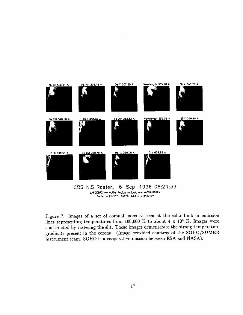
Observing Wavelengths and Spectral Resolution
With the optical telescope/magnetograph, we try to obtain information on the
velocity field and dynamics of fine structures at the photospheric and chromo-
spheric levels and the detailed vector magnetic field in the photosphere. Differ-
ent wavelengths should be used to cover these different observables. Table 2 lists
primary wavelengths and associated spectral lines that are being considered for
the telescope. Information on the photospheric magnetic field, which we con-
sider to be of the highest priority, will be obtained by measuring polarization
in absorption spectra, which is due to the Zeeman effect. The width of the Fe I
6303 ._ line, which is optimally sensitive to magnetic field, is about 100 m,_ and
so we could in principle estimate the field strength by measuring polarizations
with a comparable spectral resolution. However, the polarization depends on
the temperature structure and velocity field of the solar atmosphere, requiring
us to observe the line profiles with much better spectral resolution. Our targetspectral resolution is _25 mA.
34
Table 2: Primary Observing Wavelengths
,_ (._) Ion Observable Focal Plane3933
4305
5173
5250
5576
6302/6303
6563
Ca II (K)G-band (CH)
Mg I
FeI
FeI
FeI
. I (Ha)
chromospheric heatingdynamics of granules, structureof faculae
chromospheric magnetic field(ge.t f =1.75 )
photospheric magnetic field(gel/=3,0)photospheric velocity field(geH =0)photospheric magnetic field(gesJ =2.5)chromospheric structureHo_ flare
interference filterinterference filter
narrow-band filter
narrow-band filter
narrow-band filter
spectrograph
narrow-band filter
• Time Resolution and Continuity of Observations
The characteristic time scale that controls solar surface phenomena has a wide
range of gl minute to several months. For example, convective cells in granu-
lation change with the time scale of a minute. The yet undetected waves (such
as Alfven waves) that are excited in the convection zone and propagate into the
corona have estimated periodicities of a few tens of seconds to a few minutes.
The time scale of emerging flux is about 30 minutes. Global changes in active
regions take place with the time scale of several hours, as seen in X-ray obser-
vations. Active region evolution/diffusion has a time scale of a week to several
months. Generally, phenomena on small (large) spatial scales have short (long)
time scales. Therefore, we envision our time resolution to be about 10 seconds
(corresponding to the time needed for sound waves in the photosphere to cross
the distance of one pixel) for observations in a small field of view and several
minutes to 2 hours for observations that cover a whole active region. The Sun-
synchronous orbit ensures continuous observations of an active region while it
crosses the disk (up to 2 weeks).
• Precision of Polarization Measurement
Our ability to measure weaker field and thus to detect smaller changes in energy
increases with the precision to measure polarizations in an absorption line. The
S/N ratio in the measurement is proportional to square root of the number of
photons, so improvement of precision requires long integration times to get more
photons. We aim at achieving precision of 0.1-0.2 % per pixel. This allows us
35

Table 3: Filter Optics and Spectrograph
Item Filter Optics Spectrograph OpticsMeasuredScannedData Cube
Spectralresolution
Advantage
Disadvantage
2D spacewavelength2D space x polarization x wave-length x time70-100 m._ (narrow-band filter),10-20 _ (interference filter)Obtain 2D information in a shorttime
Hard to attain high spectral res-olution or line profiles
1D space x wavelength1D space
(1D space x wavelength) x polar-ization x 1D space x time25 m/_
Obtain line profiles with highspectral resolution and accuratedetermination of the magneticfieldSlow to scan
to observe the longitudinal magnetic field down to 2 G. In this way, we will
probably be able to detect changes in the magnetic field due to minor flares.
• Two Focal Plane Packages - Filter and Spectrograph -
As explained above, we are quite ambitious about what we hope to achieve
with the optical telescope/magnetograph. It is clearly impossible for one focal
plane package to cover all the objectives. Therefore we propose to have two
focal plane instruments, filter optics and spectrograph optics, to which we as-
sign complementary roles. The spectral resolution of the filter optics is only
_100 m]k, not enough for high precision polarization measurements. But the
filter optics can simultaneously produce wide field-of-view images and provide
high time resolution observations. The spectrograph needs time for scanning
different locations to produce a map, but it can provide line profiles with high
spectral resolution, which are essential in obtaining accurate vector magneticfield values. Table 3 summarizes characteristics of both the instruments. We
expect to achieve our various scientific objectives by using the two packages in
accordance with the observing targets. In addition, we plan to introduce table-
based flexible observing sequences, in order to achieve the best performance of
the telescope for the individual targets.
36

Table 4: Specifications of the Optical Telescope/Magnetograph
Optical System
Telescope Tube
Focal Plane Package
Objective
Observing Wavelength
Wavelength Switch
Spectral ResolutionCCD
Pixel Size
A/D ConverterPlate Scale
FOV
Standard ExposureTime Resolution
Aplanatic Gregorian, 50 cm diameter, F/10.5
CFRP (graphite epoxy), truss structureNarrow-band filter
Mapping of magneticand velocity fields4500-6600 -_
Rotating waveplate or
piezo electric actuator0.1/_ at 6000/_
2048x2048
(9 #m) 210 bit
0'/1/pixel
(200-)2200 msee
10 sac (best)
Interference filter
High spatial resolu-
tion imaging3933, 4305/_Filter wheel
]0-20 h2048 x 2048
(9 _m) _10 bit
{Y/1/pixel
(200,,)0.1-100 msec
several sac (best)
Spectrograph
High precision mag-netic observations
6203/6303/_
25 m/_ at 6000 ._.
2048 x 2048 (TBD)
9/_m (TBD)10 bit
if/1 x25 m/_/pixel150" x 0'/2
300 msec
100 min/AR
Observing Coverage
Image stabilization
Changing FOV
CPU
Frame MemoryAmount of
uncompressed data
Number of imagesobtained
Data compression
Size
WeightLowest
eigen-frequency
Moving parts
Temperature control
Continuous observing in Sun-synchronous orbit
Use attitude control and tip tilt mirror to achieve lY/02 per 10 sac.
Spacecraft attitude control (in addition, tracking of a region usingsolar rotation is under consideration.)
Equivalent of 80C386 for control and on-board processing
,_30 Mbytes (16 Mbit DRAM)Data production rate: average--740 kbps, maximum-TBD kbps,total amount of data: 4.4 Gbits per orbit
About 440 lk x lk images per orbit
2 x 2, 4 x 4 CCD on-chip pixel summation, bit compression with con-
sideration of photon noise, reduction of the amount of data by using
partial-frame mode, DPCM and JPEG compressions by DPexternal: 100 cm x 100 cm x 300 cm
goal: 150 kg (maximum system distribution: 200 kg15 Hz (assuming that the sub-system requirement is satisfied)
filer wheel, focus adjustment mechanism, counter wheel (stepping
motor) for stabilizing the satellite, shutter (DC motor), tip tilt
mirror and scan mirror (piezo electric actuator)
nominal: Sun light, non-nominal: Night-time heater (TBD)
37

Optical Telescope Schematic
Polarization
analyzer
Tip-Tiltmirror ('I'BD)
cone
CCD 1 Camera
Counter wheel 1 1_
Counter wheel 2 _]
Blockingot filter filter wheel
X 2 Interferencefilter wheel
Collimator
Polarizingbeam splitter
Relay lens
. Llltmw tens• _i,. Spectrograph _
Slit
;canning mirror
2
Shutter
Figure 18: Optical Telescope Schematic. See text for more complete discussion.
The polarization modulator, in front of the tip-tilt mirror, is labeled polarization
analyzer in this drawing; in fact, the polarizing beam splitter serves as the polarization
analyzer.
38

Table 5: Detailed Parameters of the Telescope Optics
Primary Mirror
Material and Weight
Surface Accuracy
Support
Secondary Mirror
Synthesized focal
lengthDistance betweenthe mirrors
Back focal length
Secondary
magnificationFOV
Tolerance of position-
ing the secondary
Heat dump mirror
55 cm diameter, 50 cm effective aperture, f: 1.5 m, F/3
ULE or Zero-Dur light mirror (_11 kg) or CFRP+ULE
_/10 p-v, A/40 rms (including deformation due to gravity)
Multi-point (,,,9) support from back, 3 interfaces on the tele-
scope structure, stress relief mechanism with springs17 cm diameter
525 cm, F/10.5 (secondary focus)
200cm
Maximum (200") 2
Along the optical axis: within 4-300 pm, compensated by thefocus adjustment mechanism, stability along the optical axis:
within 4-3/_m/TBD interval, inclination: within 4-40"
45 deg fiat mirror, aperture: 0.4 cm, external diameter shorteraxis Din: 3.2 cm, shorter axis: 4.5 cm, diameter of the shadow
of the secondary mirror D0: 4.2 cm, margin (D,-Dm)/2:5=0.5 cm
3.1.1 Optical TelescoPe System 1
We show the layout in Figure 18 and give detailed parameters in Tables 4 and 5. We
have established the following baseline for the design:
• The telescope is Gregorian, on the basis of considerations of thermal design. We
place a heat dump mirror at the primary focus, excluding sunlight from outside
the final field of view.
• The effective aperture is 50 cm, from the requirement of spatial resolution.
• We do not put a tilt mirror in front of the polarization calibration wheel, in order
to minimize instrumental polarization and t'o accomplish the 0.1% precision.
• To relax the positioning tolerance with the focal plane package, a lens is placed
in the center of the primary mirror, collimating the output light.
We include in Table 5 the positioning tolerance for the secondary mirror. We
should make sure that the secondary mirror be positioned within 5=0.1 mm (decenter:
1Abstracted from the Japanese proposal to ISAS
39

offset perpendicular from the optical axis) and 4-40" (tilt: inclination from the optical
axis) both in the ground test environment (under 1 G) and in orbit. We plan to absorb
this accuracy in the telescope structure design, but if this turns out to be impossible
we will put a mechanism to adjust the secondary position. The defocus tolerance
of 4-3 #m is worked ont on the assumption of a fixed secondary, and thus should
not be regarded as a requirement, as is. Rather it should be regarded as a long-
term stability requirement. Therefore it is essential to have a mechanism to adjust
the focus, to compensate possible defocus of the secondary mirror and offsets of the
components in the focal plane package. With such a mechanism we can cope with the
offset of focus caused during launch and secular variations. Apart from vibrations and
shocks at launch and initial in-orbit deformation, other causes of focus changes include
temperature variations due to seasonal variations of solar radiation input, but this
change is slow enough. The positional tolerance of the secondary is set to +300 #m,
an amount which cannot be compensated by the focus adjustment mechanism in the
presence of spherical aberration. As the focus adjustment mechanism, we are thinking
of the possibility of moving the collimator lens in the focal plane package or inserting
two wedge-like glass plates in the converging optical paths. The accompanying spot
diagram in Figure 19 shows the high quality imaging that is expected.
We will choose the mirror material with due consideration in terms of the polishing
quality, thermal, mechanical and radiation properties, previous space applications,
etc. The present candidates are ULE (ULE7971 of Corning), Zero-Dur and new
material that consists of glass with small thermal expansion coefficients placed on
CFRP. We plan to adopt either honeycomb or eggcrate structure to reduce the weight
of the primary mirror. The weight of the primary mirror is about 11 kg if either ULE
or Zero-Dur is used. Thermal deformation is quite small for ULE, as shown in Table
6. So far, the combination of CFRP+low expansion glass is quite unique in the sense
that it can satisfy low thermal deformation, high thermal conductivity, light weight
and high mechanical strength. We have obtained a 25 cm diameter trial sample and
confirmed good surface accuracy in addition to the above properties. The remaining
problem is a small amount of warp due to moisture and the way it is supported. Our
action items include studying the mechanism to dump heat, deformation and surface
accuracy under 1 G gravity, stress relief installation to the telescope body, required
centering accuracy, and optimizing mechanical strength and resonant frequency underthe M-V vibration environment.
Positioning tolerance of the secondary mirror was obtained through a ray trace
with the requirement that everywhere in the 200"×200 '1 field of view, aberration
(RMS radius) be considerably (less than 1/2x/3) smaller than the Airy disk of a
50 cm aperture primary (0':25 radius at 5000 _).
XAD=radius of Airy Disk (0.25" at 5000 ._)
4O

I
J!
!
l
.,._',-..
% .j°_ •.
i. .. ill
%iH . i
Figure 19: Spot diagrams at the optical axis and 100" off axis. The 4 corner pixels
are located 140" away from the axis. Each box corresponds to the pixel size (0'._1).
41

Table 6: Thermal Deformation of the ULE mirror
Pattern of temperaturechange
Deviation from the presettemperature AT=+50 KTemperature difference be-tween the two sides, simu-lation using heat input of32W/50cm¢
Cellular temperature gradi-ent, simulation using heat in-put of 32W/50cm¢
type ofdeformation
similar
warp
scale-like
effect
spherical aberration
spherical aberration
surface unevenness
0.001 AD 1
0.03 AD
A/10 s
Radial temperature gradient, bend spherical aberration very smalldT/dr=-50 K/25cm
3.1.2 Filter Vector Magnetograph and Imager
General Goals and Specifications
Two filter instruments are discussed here; they will share the optical telescope
focal plane with the spectro-polarimeter. For discussion purposes, these systems are
referred to as the broad-band filter (BBF), narrow-band filter (NBF), and spectro-
polarimeter (SP). The details of how to best integrate and share the resources available
behind the telescope focal plane are the subject of ongoing discussions among US and
Japanese investigators. However, some goals are clear at the present stage of thosediscussions.
The BBF should preserve the highest angular resolution of which the telescope is
capable while simultaneously covering the entire high-quality field of view (i.e. 200").
The photometric precision and accuracy should be no worse than a few tenths of a
per cent in a single exposure. These requirements imply a ccd camera with approx-
imately 0.1" pixels and a format of about 2048 by 2048 pixels. The spectral ranges
to be covered should include the chromosphere (e.g. 393.3 am), the temperature
minimum (e.g. 430.5 nm), and a clean continuum (e.g. 451.9 am). The spectral
resolution should be at least 400. Exposure times should be short enough to reduce
any photometric errors arising from the proper motion or evolution of solar featuresto less than 1%.
The NBF should also meet the same goals as the BBF except for providing higher
spectral resolution (at least 50000), a selection of spectrum lines, rapid tunability,
and polarization selectability. At least one spectrum line should be chosen to yield
high quality photospheric vector magnetic field information. Another spectrum line
42
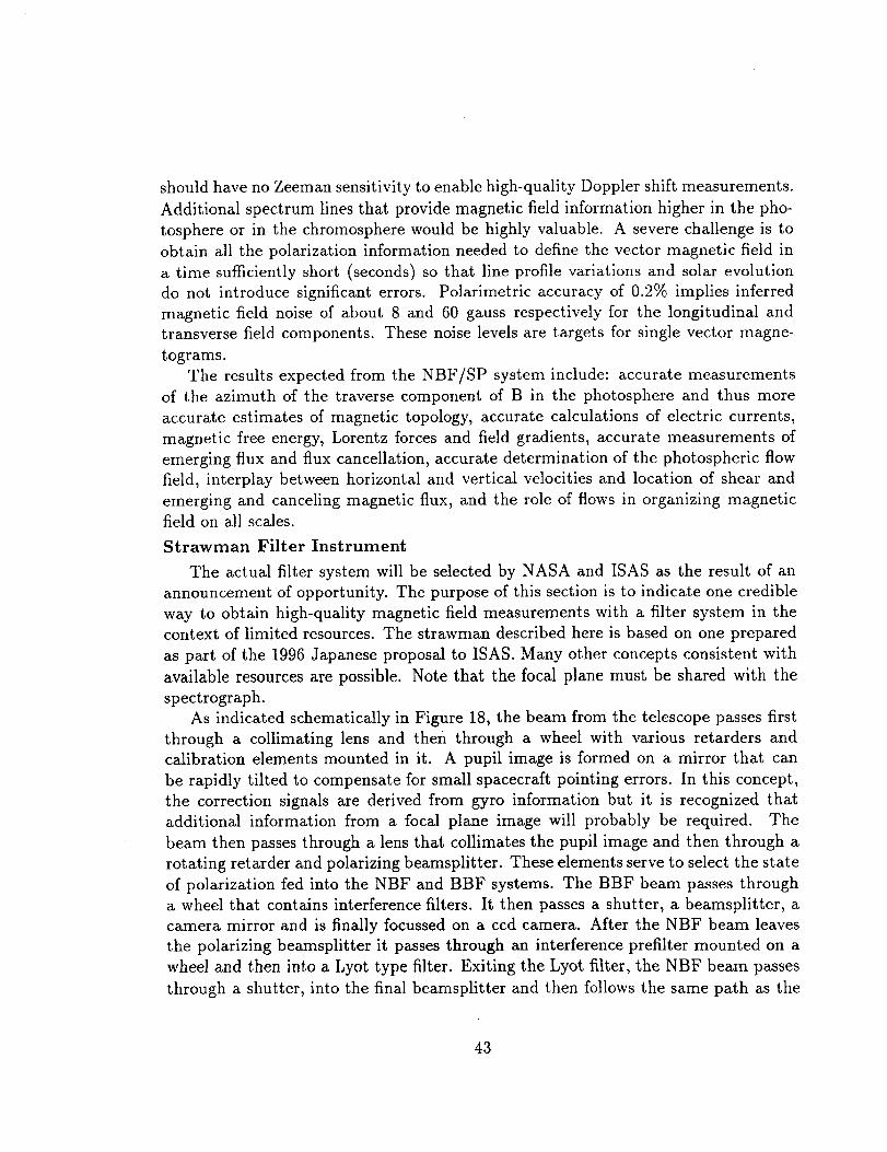
shouldhavenoZeemansensitivity to enablehigh-quality Doppler shift measurements.Additional spectrum linesthat provide magnetic field information higher in the pho-tosphereor in the chromospherewould be highly valuable. A severechallengeis toobtain all the polarization information neededto define the vector magnetic field in
a time sufficiently short (seconds) so that line profile variations and solar evolution
do not introduce significant errors. Polarimetric accuracy of 0.2070 implies inferred
magnetic field noise of about 8 and 60 gauss respectively for the longitudinal and
transverse field components. These noise levels are targets for single vector magne-
tograms.
The results expected from the NBF/SP system include: accurate measurements
of the azimuth of the traverse component of B in the photosphere and thus more
accurate estimates of magnetic topology, accurate calculations of electric currents,
magnetic free energy, Lorentz forces and field gradients, accurate measurements of
emerging flux and flux cancellation, accurate determination of the photospheric flow
field, interplay between horizontal and vertical velocities and location of shear and
emerging and canceling magnetic flux, and the role of flows in organizing magnetic
field on all scales.
Strawman Filter Instrument
The actual filter system will be selected by NASA and ISAS as the result of an
announcement of opportunity. The purpose of this section is to indicate one credible
way to obtain high-quality magnetic field measurements with a filter system in the
context of limited resources. The strawman described here is based on one prepared
as part of the 1996 Japanese proposal to ISAS. Many other concepts consistent with
available resources are possible. Note that the focal plane must be shared with the
spectrograph.
As indicated schematically in Figure 18, the beam from the telescope passes first
through a collimating lens and then through a wheel with various retarders and
calibration elements mounted in it. A pupil image is formed on a mirror that can
be rapidly tilted to compensate for small spacecraft pointing errors. In this concept,
the correction signals are derived from gyro information but it is recognized that
additional information from a focal plane image will probably be required. The
beam then passes through a lens that collimates the pupil image and then through a
rotating retarder and polarizing beamsplitter. These elements serve to select the state
of polarization fed into the NBF and BBF systems. The BBF beam passes through
a wheel that contains interference filters. It then passes a shutter, a beamsplitter, a
camera mirror and is finally focussed on a ccd camera. After the NBF beam leaves
the polarizing beamsplitter it passes through an interference prefilter mounted on a
wheel and then into a Lyot type filter. Exiting the Lyot filter, the NBF beam passes
through a shutter, into the final beamsplitter and then follows the same path as the
43

BBF to the ccd.
The ccd camera has 2048 by 2048 pixels with each 9 by 9/_m pixel covering 0'._1. A
10 bit A/D converter will provide adequate dynamic range and signal to noise ratio.
Exposure times will be 0.1 to 100 msec for the BBF and about 200 msec for the NBF.
Each full-frame exposure will produce raw images of 42 Mbits. On-chip binning and
partial frame readout will be provided. The data handling system will be able to do
simple arithmetic on stored images and both lossless and lossy image compression.
These techniques are required since without them only 47 raw images per orbit could
be downlinked neglecting the SP entirely.
A representative observation sequence might consist of one BBF frame, one frame
each in the red, center, and blue wings of the H-alpha line, and four frames each
in the blue and red wings of the magnetograph line (four states of polarization), for
a total of 12 frames. Such a sequence would be repeated every few minutes. Note
that on-board processing and compression make such a program compatible with the
available telemetry.
Heritage
Filter-based imaging and magnetograph systems have a long heritage. Ground-
based systems of this sort have been in service for more than 20 years. A current
count shows at least ten filter vector magnetograph instruments operating at ground-
based observatories. Three additional ones are reported to be under construction and
two have been prepared for flights on large, balloon-borne telescopes. A filter mag-
netograph (longitudinal component only) is on board SOHO and provides excellent
measurements. Most of the instruments use Lyot filters but a few use Fabry-Perot
narrow band filters. A couple are hybrids that combine Lyot and Michelson filter
elements. Polarization modulation is done by variable retarders including KDP and
liquid crystal devices, rotating fixed-value retarders, and, in one case a fixed beam-
splitter. The polarimetric noise is a few per mil typically. Most of the systems use
pass bands of about 0.1 A and most operate with the 6302 A line. Other popularlines are 5324 and 5250/_.
3.1.3 Spectro-Polarimeter
The Importance of Spectrographic Stokes Polarimetry from Space
Quantitative measurements of the photospheric vector magnetic field are funda-
mentally important to the science goals of Solar-B. Our ability to infer this funda-
mental property of the solar atmosphere from polarimetric observations depends in
a very sensitive manner upon the completeness and precision of the polarimetric ob-
servations. It is crucially important to take advantage of the complete information
contained in the spectrally resolved profiles of Zeeman-sensitive solar absorption lines
44

(the "Stokes polarization profiles"). Without such information it is generally not pos-
sible to infer the strength and orientation of the magnetic field with high precision
and quantitative detail, especially in regions outside of sunspots. Because many of
the science goals of Solar-B hinge upon our ability to make quantitative measure-
ments of the field (vertical current densities and true magnetic flux measurements
are two obvious examples of required measurements), the baseline concept for the
complement of instrumentation aboard Solar-B includes a spectrographic instrument
whose primary goal is the precision measurement of polarized solar line profiles. Fur-
thermore, this instrument would perform spatial maps of the solar surface in order to
construct detailed, high resolution, quantitative surface maps of the vector magnetic
field, maps of related thermodynamic properties of the solar atmosphere, and even
point-by-point gradients of these quantities along the line-of-sight from asymmetries
of the line profiles.
To date, no instrument capable of vector magnetometry has been flown in space.
In fact, it is only within the past few years that the instrumentation with the spec-
trographic capability described above, along with the analysis methods needed to in-
terpret such data, have been demonstrated through ground-based observations. The
recent experience with ground-based spectrograph polarimeters has set a new stan-
dard for both precision and angular resolution of vector magnetic fields, and numerous
discoveries regarding the nature of the magnetic field, its evolution, and its influence
on the solar atmosphere are forthcoming. Figure 20 shows a typical set of polarization
images from the ground-based Advanced Stokes Polarimeter. The fundamental data
from such a polarimeter are spectral images of the solar photospheric absorption lines
in intensity (Stokes I), two orthogonal states of linear polarization (Stokes Q, U), and
right- minus left-handed circular polarization (Stokes V), as shown in the lower four
panels of this figure. The Q, U profiles are basically symmetric about the centers of
the Zeeman-sensitive Fe I lines at 6302/_, indicating the presence of magnetic fields
transverse to the line-of-sight. The Stokes V line profiles are basically antisymmetric.
The three images at the top of the figure represent, from left to right, continuum in-
tensity, Stokes V in the wing of one of the lines, and Doppler velocity. They indicate
the location of the spectrograph slit corresponding to the spectral images below. The
sunspot appears dark at all wavelengths in the Stokes I image. Narrow spectrum
lines due to 02 absorption in the Earth's atmosphere produce no measurable polar-
ization of the spectra. They would be absent in Solar-B spectra. Notable in these
spectra is a very small location of supersonic (14 km s-1) downflow visible in the
polarization spectra Q, U, V (upper arrow in the Doppler image). Such events would
not be recognized in filter magnetograph images. Full spectral polarization profiles of
significantly higher angular resolution and polarimetric precision will be obtained by
the Solar-B spectro-polarimeter. Data of that quality is necessary to extract precise
measures of the vector magnetic field, and other important thermodynamic properties
45

of the magnetized solar atmosphere. Figure 3 illustrates the spectacular results that
we expect to be able to derive on a regular basis from such data.
Stokes polarization measurements are however severely limited by the nature of
observing through the turbulent Earth's atmosphere. In order to attain the requisite
Signal-to-Noise ratio (S/N > 1000) integration times must be longer than about
3 seconds even with rather large aperture ground-based solar telescopes. With such
restrictions, atmospheric seeing sets a fundamental limit - about 1 arcsecond - on the
angular resolution achievable with ground based instrumentation, thereby masking
much of the information about the small-scale structure of the vector magnetic field.
Perhaps more importantly, the 1 arcsecond image quality is quite intermittent, and
observational sequences are always compromised by the day/night cycle and by clouds.
It is therefore not possible to record the evolutionary history of solar flux elements
from the ground with the required precision and angular resolution. For these reasons
many crucial observational data on the evolution of the magnetic fields in active
regions probably cannot be derived from ground-based measurements.
We are now at a juncture where we understand in detail the the scientific require-
ments of vector magnetic field measurements, how to carry out the needed precision
polarimetric observations from a space platform, and how to interpret the data once
it is in hand. It is clear that the entirely new class of observational data afforded
by a spectrographic polarimeter in space, operated in concert with the filter vector
magnetograph, will represent an unprecedented advance for solar physics in defining
the observational state of the solar magnetic field. At this moment we are presented
with an extraordinary opportunity: an opportunity which may be seized with rela-
tively modest resources. Such an instrument, along with the suggested complement
of other instruments aboard Solar-B, will deliver data which will have a tremendous
and lasting impact on the discipline.
Requirements for Precision Stokes Polarimetry
Requirements for precision polarimetry place strong constraints on the mode of
data acquisition. Some of the most important issues are listed below.
• Signal-to-Noise Ratio: For analysis of active region fields, a S/N in the range >
1000 appears to be necessary for inference and interpretation of vector fields. For
detailed studies of individual flux tubes, or for studies of the quiet internetwork
fields, an even larger S/N may be required.
• Simultaneous Polarization Measurements in Two Spectral Lines: It is essential
that two spectral lines with similar response to thermodynamic structure, but
differing response to the Zeeman effect, be measured simultaneously.
• Rapid Modulation of the Polarization: The S/N requirements also dictate that
a full measurement of Stokes polarization profiles takes place in a time interval
46

HAO/NSO Advanced Stokes Polarimeter
19 June 1992-NOAA 7201
15:09 UT Lat 24 Long -5
rain max
3035 I (ADU) 43629
-0.0273 Q/Imax 0.0206
-0.0286 Ullmax 0.0543
-0.1128 V/Imax 0.1033
i Q
U V
Figure 20: Precision spectro-polarimetric observations of the Zeeman-sensitive Fe Ilines at 6301 and 6302/_..
47

short enough that there is no appreciable "crosstalk" from intensity into po-larization due to evolution of the solar scene.Given expectedproper motionsof solar photospheric featuresof a few km/sec, we require that each completemeasurementof polarization be executedwithin lessthan one secondin orderto achieve a polarization accuracy of 0.001.
Efficient Use of Available Light: The strong requirements on S/N dictate that
efficient use of the available light flux be made so that maps of active regions
may be carried out in a time compatible with their evolutionary time scales.
Contextual Filter Observations: The spectrographic observations are limited
spatially by the width of the slit. Requirements of the S/N and telemetry
prevent large, detailed spatial maps of spectro-polarimetric observations to be
acquired in a time short compared with the evolution of the solar scene. It
is therefore necessary to have BOTH the spectro-polarimeter AND the filter
magnetograph operating simultaneously, in concert. In this way, the precision
magnetic field measurements from the spectro-polarimeter can be placed into
their proper context of the evolution of the solar scene. Such combined measure-
ments are essential to achieve many of the fundamental science goals of Solar-B;
for example, in order to both follow the spatial migration of active region flux
and to make precise quantitative measurements of the individual field elements.
Elements of the Optical Spectro-Polarimeter
Below we present a strawman concept for the visible light spectrograph, shown
schematically in Figure 18. The actual spectro-polarimeter system will be selected
by NASA and ISAS as the result of an announcement of opportunity. This concept
demonstrates that it is possible to achieve precision measurement of magnetic fields
with a modest and simple spectrograph. This concept is only intended as an example
to illustrate this feasibility. It is based on studies carried out over the past few years,
and a similar system is described in the 1996 Japanese proposal to ISAS. Many other
concepts consistent with available resources are possible.
The strawman spectro-polarimeter allows measurement of the full state of po-
larization in spectral lines formed in the solar photosphere, with sufficient spectral
resolution to resolve the subtle features of the Stokes polarization profiles, simulta-
neously in two nearby spectral lines. It also permits one to acquire measurements of
spectra and polarization in the core and wings of the Ca II H-line (3968 A). The H-line
measurements are required to connect the photospheric field measurements smoothly
through the chromosphere to the upper layers sampled by the other instrumentation
on Solar-B. Because of the seeing-free space environment, many of the difficulties
associated with ground-based Stokes polarimetry may be relaxed for a space-borne
48

polarimeter, permitting a smaller, simpler, slower instrument than neededon the
ground. Some of the critical elements of this system are described below.
• Polarization Modulator: The polarization modulator is placed as far forward
in the optical path as practical in order to minimize the influence of optical
elements on the small solar polarization signals to be detected. This device
must change the state of polarization of the incident light in a periodic manner.
The strawman polarimeter has a continuously rotating fixed retarder with 3/8
wave retardance at the wavelength of the chosen Zeeman-sensitive Fe I line pair
at 6302 A. The rotation rate would be approximately 0.94 Hz. An alternate
candidate for a polarization modulator is a liquid crystal variable retarder which
modulates the retardance via an applied electric field. The former modulation
scheme requires a mechanism to rotate the retarder. The latter scheme would
require a separate set of polarization calibration optics, in the optical path
ahead of the modulator, which could be introduced occasionally to monitor the
performance of the liquid crystal.
• Tip-Tilt Image Motion Compensator: Even a tiny translational motion of the
solar image at the detector could produce a spurious polarization signal at the
limit of the required polarization sensitivity. Gross image translation should
be stabilized at the level of about 0.003 arcseconds within the typical time
of modulation of the polarization (0.3 seconds). The tip-tilt mirror shown in
Figure 18 will compensate for small excursions of the image due to spacecraft
drift, vibration from onboard mechanisms, and wobble of the image due to the
rotating waveplate. The filter instruments place similar requirements on image
stabilization. Note that the solar scene observed at this high resolution will
evolve significantly in a few seconds. The tracking cannot compensate for this
motion, but polarization errors arising from the evolving solar scene will be
smaller than the desired accuracy, 0.001, when the modulation/demodulation
of the polarization is carried out at 15 Hz.
• Polarizing Beam Splitter: The image is divided between the spectrograph and
the filter instrument via a polarizing beam splitter, which performs several
functions. First, it permits simultaneous operation of both systems. Second, it
acts as an analyzer for the polarization system, both for the spectrograph and
the filtergraph, thus none of the photons available for polarization analysis are
wasted in an absorbing polarizer. Third, it acts as the initial polarizer element
for the Lyot filter.
• Scanning Mirror: This mirror functions to translate the image of the Sun across
the entrance slit of the spectrograph in order to produce spatial maps of the
magnetic field and related atmospheric parameters.
49

• Spectrograph: The simple Littrow configuration, with a total length of about
1.5 m, provides adequate spectral resolution (25 mA) for vector field measure-
ments. The shutter wheel mechanism provides both for dark-level calibration,
and contains blocking filters for two wavelengths, 6302 and 3968 A.
CCD Cameras: The CCD cameras must be read at high rates (15 Hz is the
baseline) for the two reasons given above: l) modulation of the polarization
must proceed rapidly in order to minimize the spurious polarization signals from
the evolving solar scene, and 2) high S/N requirements demand that photons not
be wasted. In the focal plane of the spectrograph the pixels are 0.2 arcseconds
by 25 mA. The camera should be a frame-transfer device to permit continuous
(un-shuttered) operation, and have low read noise (<60 e-) at the desired 15
Hz read rate in order to achieve measurements dominated by photon sampling
statistics. The active area of the chip should be at least 1000 X 200 pixels.
Two cameras are required in the focal plane: one for the precision photospheric
vector field measurements at 6302 A, and one for the chromospheric spectra of
the Ca II H-line at 3968 A. A dichroic beamsplitter preceding these two cameras
relay the appropriate wavelength regions to each CCD, and unwanted spectralorders are rejected by broad-band interference filters in front of each camera.
Demodulation/Accumulation Electronics: The CCD camera is read and accu-
mulated into several buffers simultaneously during about 3 seconds in order
to build up the required S/N. A processing system dedicated to the spectro-
polarimeter will be needed to carry out the demodulation, to cull out the desired
spectral and spatial windows from the entire image of each CCD camera, and
to apply the lossless or lossy data compression.
Data Rate Considerations
• Maximum Raw Data Rate: 1000 spatial x 80 spectral pixels x 4 Stokes param-
eters x 2 bytes/pixel every 3 seconds = 2.1 x l0 s bytes/sec.
• Maximum Raw Data Volume: 1.2 Gbyte/orbit
• Maximum Rate after Data Compression: 120 Mbyte/orbit
• Routine data compression: about 90% is possible without serious degradationof inferred magnetic field parameters.
5O

Table 7: Solar-B Spectro-Polarimeter
Continuum S/N of typical observation
Polarimetric precision
Spectral Coverage
Spatial pixel sizeSpectral samplingSpatial coverage along slitSpectral coverage of each photosphericline
Polarization sampling rate (frame rate)Duration for one spectral measurement
> 1000:1
comparable to noise, i.e. 0.001
Simultaneous coverage of two spectrallines (e.g. Fe I 630.15,630.25 nm)
(Additional coverage of CaII H-line, if
possible)0.2"
< 2.5 pm> 200"> 0.08 nm
> 15 Hz
< 3 sec.
Critical Design Tradeoffs
Photon Flux: Calculations based on modern, efficient CCD detectors and other
efficient optical elements only becoming available in the last two years, along
with the simple optical system of the strawman Solax-B spectro-polaximeter,
demonstrate the the strawman system can achieve the required S/N. Addition-
ally, these photon flux estimates have been verified by comparison with actual
signal levels from the Advanced Stokes Polaximeter. The projected photon flux
remains a serious design consideration of any such precision polaximeter, and
any changes of the optical system upstream of the spectro-polaximeter should
be weighed in consideration of the stringent S/N requirements.
Polarization Modulator: Two choices for viable polarization modulators have
been considered: a rotating optical retarder and Liquid Crystal Variable Re-
tarders (LCVRs). The rotating optical retarder is robust, but requires a me-
chanical device and introduces a small, slow, but probably manageable wobble
to the beam that must be compensated by an active image motion compen-
sation. LCVRs require no moving parts and do not disturb the beam, but
candidate devices axe rapidly degraded by UV radiation, and it is not clear
how reproducibly their retardance can be tuned, leading to questions regard-
ing the precision of polaximetric measurements possible with such devices. In
any case, image motion compensation will be necessary for the optical tele-
scope and instrumentation and it is expected that the high precision needed
can be achieved. If the modulator is placed early in the optical path (as is
ideally done to allow precision polarimetry), the filter magnetograph, like the
51

spectro-polarimeter,wouldneedto havea detector capableof demodulating the
encoded polarization signal.
Spatial coverage: The number of CCD pixels along the slit determines one
dimension of the spatial maps from such a device. For 1000 pixels, a coverage
of 200" would be possible. This is acceptable for active region studies. Data rate
and S/N dictate how rapidly such data can be taken. A reasonable cadence for
stepping the slit of 3 seconds (S/N = 1000:1) implies that about 50 min would
be required to build up a map of an area (200 x 200") with if:2 steps. Of course,
different scientific objectives could dictate larger step sizes, or scans covering asmaller area of the solar surface.
Data Rate: Any polarimeter such as this will generate a large quantity of data.
The instrument outlined in Table 7 will produce a raw data stream with a
rate of about 2 M-bit/sec. On-board data compression would be possible to
reduce this data flow by a factor of 5-10. Still, this instrument alone could
produce data at a continuous rate of at least 200K-bit per second. This is a
serious consideration, but this data rate, if not continuous, at minimum would
be necessary for extended periods in order to do the science. It should be noted
also that considerable on-board processing power will be needed to achieve this
level of data compression.
Spectro-Polarimeter Heritage
This instrument has no space heritage, but considerable experience is now in hand
from related ground-based instrumentation (the Advanced Stokes Polarimeter: ASP
and its predecessors; the University of Hawaii spectro-polarimeter.) The scientific
success of ASP and the experience gained with this device has led naturally to a
need for more powerful space instrumentation. The need for larger field-of-view than
provided by ASP, and the need for observations not limited to a few brief observing
runs per year has led to the proposal by the National Solar Observatory for a new
ground-based spectro-polarimeter for synoptic studies (as part of the SOLIS facility.)
The SOLIS concept has many features in common with the strawman Solar-B spectro-
polarimeter presented here. This demonstrates both the scientific need for precision
polarimetry and the viability of the overall concept.
It should also be emphasized that a considerable effort has been devoted during
the past decade to develop the tools to analyze this data in order to extract vector
magnetic field measurements. These techniques are in hand, and are in routine usage.
Furthermore, several groups around the world are developing more advanced analysis
techniques which now permit the determination of gradients of physical parameters,
including the magnetic field vector, along the line of sight.
52

3.2 X-Ray Telescope
The X-ray Telescope is the second major component of Solar-B. It will provide, at
a minimum, the detailed observations of the high temperature material in the Sun's
outer atmosphere, which in this context includes both the transition region and the
corona, in the form of high resolution,full disk images. These images will permit the
study of both the dynamics of fine scale coronal phenomena, for instance magnetic
reconnection and coronal heating mechanisms, while at the same time recording the
large scale global phenomena, such as coronal mass ejections, which have a direct
impact on the terrestrial system. A major objective of the X-ray Telescope, which re-
flects one of the primary objectives of Solar-B, is to observe and quantify the coronal
response to changes in the magnetic field measured in the photosphere. This connec-
tion has to be made across a relatively large separation in both space (a few seconds
of arc) and temperature (1 MK). If the connection for instance between coronal loops
and their magnetic footpoints is to be made unambiguously the instrument has to be
capable of measuring emission from material lying at least as deep in the atmosphere
as the transition region and having a temperature near 0.5 MK. At the same time
time the instrument must be capable of recording the emission from the much higher
temperature material (2-5 MK) which dominates the corona.
Based on these general objectives a set of minimum requirements for the telescope
can be established. First the telescope must have adequate sensitivity over a suffi-
ciently wide wavelength range to ensure that the coronal phenomena can be traced
back to the transition region. This specifically implies an ability to detect the emis-
sion from relatively cool structures with temperatures between 0.5 and 1.0 MK in the
presence, along the line of sight, of material at much higher temperature. Second the
instrument must have the ability to provide precise temperature diagnostics over the
temperature range from 0.5 to 10 MK. The telescope should be capable of recording
the full disk, without raster scanning, and the resulting images should have a reso-
lution defined by the detector pixel size of 1725 (or less), more than a factor of two
improvement over the Yohkoh telescope which had approximately 2':5 pixels.
In principle the requirements can be met by a telescope based on either the grazing-
incidence (soft X-rays) or the normal-incidence multilayer (XUV) mirror approach.
Each approach has its strengths and weaknesses and an instrument based on a com-
bination of both techniques deserves serious consideration. This conclusion is based
on the evidence, obtained by comparison of nearly simultaneous images from both
types of telescope, that they frequently provide a significantly different view of the
corona. Such observations may also provide the first opportunity to obtain measure-
ments of the variation of temperature across a coronal loop. Both types of telescope
have extensive space heritage. Most recently the extremely successful Soft X-ray
Telescope(SXT) on Yohkoh was of the grazing-incidence design while the Extreme
53

Fe XIX 108A
(6.3MK)
(2.0MK)
Pre-filter
Detector
(CCD)
Fe Xl 180A
(1.3MK)
Selector shutter Primary minor
Figure 21: Baseline Solar-B normal-incidence XUV telescope.
Ultraviolet Imaging Telescope (EIT) flown on the SOHO mission and the Transition
Region and Coronal Explorer (TRACE) telescope (launch 12/97) employ normal-
incidence Cassegrain telescopes, with each quadrant coated with a different multilayer
for reflecting a specific wavelength. The lines chosen correspond to low temperatures
(below 2.5 MK) and do not cover the full range of interest of Solar-B.
Whichever approach is chosen, grazing or normal-incidence, fabricating the optics
to meet the requirement on angular resolution is well within the state of the art.
Consequently the limiting factor will be set by the choice of the detector. For Solar-B
the use of 2K x 2K CCD detectors in a normal-incidence telescope has been baselined
(see Table 8 and Figure 21). Thus for a 1'.'25 pixel (a plate scale of 83'.'3 per mm) the
field of view will be 4'Z:67 which provides adequate coverage of the corona beyond the
solar limb. However it must be realized that the X-ray telescope will be aligned to
the optical telescope which will have a relatively small field of view, perhaps 5 '. If
the optical telescope is pointed at a feature near the limb then a significant fraction of
the disk will fall outside the field of view of the X-ray telescope, which is an argument
for not making the pixels smaller than 1'.'25 as this would exacerbate this effect. In
a grazing-incidence configuration (Wolter I) the required focal length to provide this
resolution is 2475 mm and the aperture of the mirror to provide a suitable collecting
area is 300 mm. Thus the envelope for this instrument can be defined as a cylinder
with a diameter of approximately 400 mm and a length of 3000 mm. The mass of
54

Table 8: Baseline Solar-B X-ray Telescope vs. Yohkoh SXT
Item
Optics
Aperture Size
Wavelengths
Detector
QEPixel Size
FormatField of View
Geometric Area
Effective Area
Temperature
Range
Solar-B (NI)Normal Incidence
Ritchey-Chretien20 cm
171 ._, 195 -_, 211+/-2/_,visibleBack-illuminated CCD
0.5
15 micron
1_._242048X2048
42_.245 cm 2
0.3 cm 2 (@171 /_)
0.7-2.0 MK + 14 MK
Yohkoh SXT (GI)
Grazing Incidence Wolter I
23 cm
3-45/_, visible
Front-illuminated CCD
0.8
18 micron
2','46
1024X102442/.0
2.62 cm 2
0.6 cm 2 (@8/_)1.5-50 MK
such a telescope, excluding electronics, should not exceed 25kg. The XUV telescope
is assumed to be a Ritchey- Chretien (i.e. an aplanatic Cassegrain) which, with a
200 mm diameter primary and having the same plate scale as the grazing-incidence
telescope, could be accommodated within a cylindrical envelope something less than
half as long as that required for that telescope, say 1250 mm, and three quarters of
the diameter (300 mm) and would have a roughly comparable mass.
The two element configuration of the XUV telescope easily accommodates a fac-
tor of four increase in the plate scale in the same envelope as the grazing-incidence
telescope, although the field of view is now less than the full Sun and the illumination
per pixel has been reduced by the square of the magnification. However the com-
bination of the two telescopes, with the XUV system mounted coaxially within the
grazing-incidence telescope, in a single instrument is physically possible and would
provide a scientifically exciting opportunity. It would have the capability for making
both high resolution observations (0'.'5 pixels) of the transition region corona inter-
face where they are most needed and full disk, SXT style images. The availability of
both narrow and broad band images would improve the coverage of the temperature
diagnostics and would allow the full range of coronal plasma temperatures from < 1
MK to >10 MK to be studied.
The ability to provide good temperature diagnostics will be critical to the quan-
titative analysis of the Solar-B data. Both telescopes rely on theoretical models of
the temperature dependence of the solar spectrum. These are then used to compute
ratios of line intensities (normal-incidence telescopes) or selected wavebands(grazing-
55

Table 9: Goals for an Imaging Spectrometer
spatial resolution
spectral/velocity resolution
temporal resolution
dynamic range
tl
10 km 8 -1
lOs
> 10a
incidence telescopes). Line ratios from the same element are used to avoid abundance
differences which makes it difficult to obtain extended temperature coverage. For in-
stance FeIX, FeXI, FeXV and FeXIX provide good diagnostics below 3 MK but are
not as good at higher temperatures where the broadband method is quite sensitive.
However the broadband method cannot be extended much below 1.8 MK, so that in
practice the the two techniques are nearly complementary.
Because of its multiple wavelength bands and the larger CCD the X-ray telescope
will be capable of generating over an order of magnitude more data for any specific
event than the Solar-A soft X-ray telescope. For instance a 2k x 2k image with 10 bit
intensity resolution contains 40 Mbits. Data compression techniques should be able
to reduce this by at least a factor of four to a level which is comparable to the Solar-
A data rate. However because of the large dynamic range present in X-ray images
standard data compression techniques are not as generally effective. Consequently
the frequency of full resolution, full disk images will have to be kept fairly low and the
telescope will have to be operated predominantly in a windowing or region of interest
mode. In this way the demands on the telemetry system can be kept within bounds.
3.3 EUV Imaging Spectrometer
The goal of Solar-B is to understand the solar photosphere and corona as a sys-
tem. The governing equations of magnetohydrodyamics specify the parameters that
determine the state of the solar atmosphere: density, velocity, temperature and the
magnetic field as a function of position and time. XUV spectroscopic diagnostics pro-
vide strong techniques to determine plasma densities, velocities and temperatures.
In addition, it is also possible to determine radiative cooling rates and elemental
abundances. A stigmatic spectrometer measures spectral line profiles emitted by the
plasmas viewed along the slit. Complete images can be obtained by rastering the slit
(SOHO/CDS, HRTS), using a slitless design as in the Skylab spectroheliograph or by
a slit/slot combination as in the SERTS spectrograph.
Plasma densities in a narrow temperature range can be determined from line in-
tensity measurements. The intensity of a spectral line is directly proportional to
56

the emissionmeasure(f n_dl). With a knowledge of the geometry of the emitting
structure the plasma density is derived. This can also be done with imaging instru-
ments. However, the measurement of individual spectral line intensities offers the
opportunity to make use of density-sensitive line intensity ratios. The intensity ratio
of certain line pairs of several iso-electronic sequence are functions of electron density
that can be accurately calculated from atomic parameters. By measuring the inten-
sity ratio of these lines, one can determine the electron density in the source region
that is nearly independent of geometrical factors such as the partitioning of the emit-
ting plasma into subresolution structures. A knowledge of the emission measure, the
electron density and the geometry of the source can then determine whether or not
unresolved fine scale structure are present. These fine scale structures are extremely
important for understanding heating through the joule dissipation of electric currents
or the viscous dissipation of highly sheared motions, which are expected to occur on
small spatial scales.
Only through the understanding of its dynamics can the solar atmosphere be
understood. A static atmosphere simply does not represent the important physical
processes responsible for the maintenance of a hot outer atmosphere and its often
explosive behavior. Clearly, this leads to a requirement to measure the velocities of
solar plasmas. The most direct measurement of velocities is through the Doppler shift
of spectra lines which can be determined almost solely by spectroscopic techniques.
Bulk motions are determined from the net shift of line profiles and the small-scale
"turbulent" motions through the width of spectral line profiles.
Spectral lines from any given ion are formed over a narrow range of temperature,
typically only a factor of 2. By measuring the intensities of lines formed over a range
of temperatures, the variation of emission measure with temperature is found and
with this the thermal energy content of the solar plasma as a function of temperature
is also known. The plasmas along any line-of-sight to the Sun passes through plasmas
at a range of temperatures and spectral line diagnostics provide a good diagnostic for
interpreting these emissions. Imaging instruments usually provide only an isothermal
or 2-temperature analysis which can over-simplify the analysis of solar phenomena.
By measuring the intensities of several spectral lines spanning a wide range of
temperature, the net radiative losses is obtained with the help of a little modeling.
The maintenance of the thermal content of the corona against its radiations losses is
central to the coronal heating problem.
A good example of the power of spectroscopic analysis are their application to
understanding the process of magnetic reconnection. This is a process that is not
well understood but always entails the reconfiguration of the magnetic topology of
the system and may also result in plasma heating and plasma ejection. It is thought
to be a central process in the conversion of energy generated by plasma motions in
the photosphere and convection zone to dynamical activity in the corona, such as
57
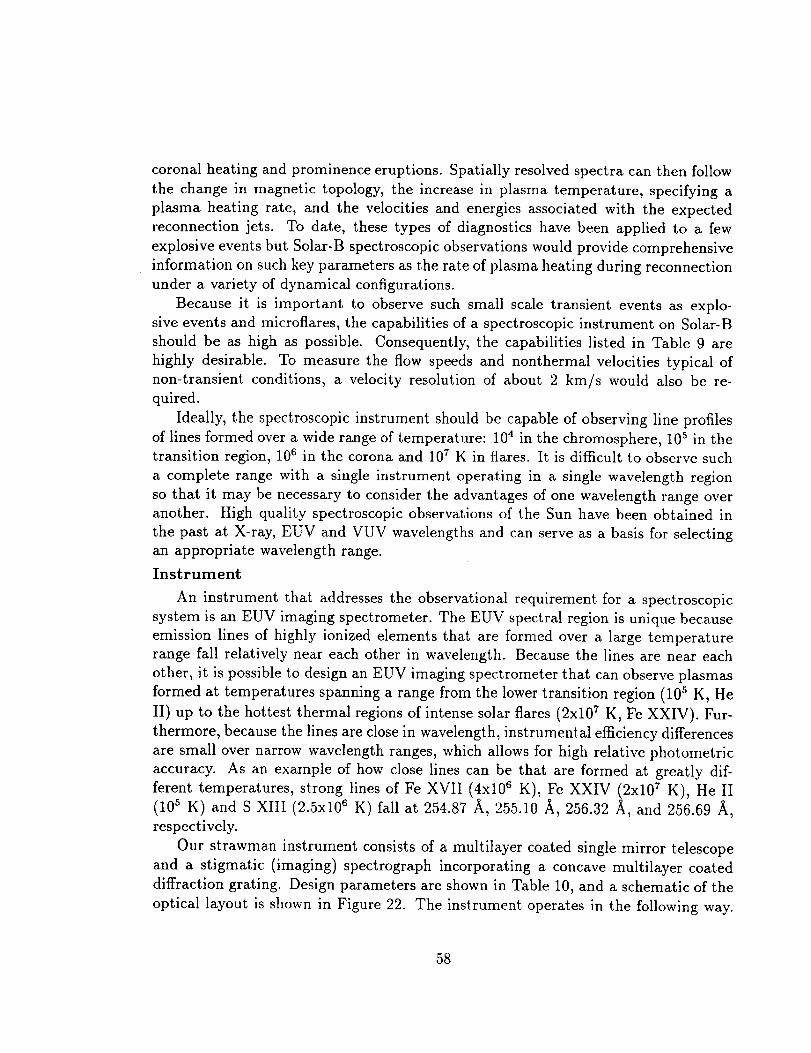
coronal heating and prominence eruptions. Spatially resolved spectra can then follow
the change in magnetic topology, the increase in plasma temperature, specifying a
plasma heating rate, and the velocities and energies associated with the expected
reconnection jets. To date, these types of diagnostics have been applied to a few
explosive events but Solar-B spectroscopic observations would provide comprehensive
information on such key parameters as the rate of plasma heating during reconnection
under a variety of dynamical configurations.
Because it is important to observe such small scale transient events as explo-
sive events and microflares, the capabilities of a spectroscopic instrument on Solar-B
should be as high as possible. Consequently, the capabilities listed in Table 9 are
highly desirable. To measure the flow speeds and nonthermal velocities typical of
non-transient conditions, a velocity resolution of about 2 km/s would also be re-
quired.
Ideally, the spectroscopic instrument should be capable of observing line profiles
of lines formed over a wide range of temperature: 104 in the chromosphere, 10 s in the
transition region, 106 in the corona and 107 K in flares. It is difficult to observe such
a complete range with a single instrument operating in a single wavelength region
so that it may be necessary to consider the advantages of one wavelength range over
another. High quality spectroscopic observations of the Sun have been obtained in
the past at X-ray, EUV and VUV wavelengths and can serve as a basis for selecting
an appropriate wavelength range.
Instrument
An instrument that addresses the observational requirement for a spectroscopic
system is an EUV imaging spectrometer. The EUV spectral region is unique because
emission lines of highly ionized elements that are formed over a large temperature
range fall relatively near each other in wavelength. Because the lines are near each
other, it is possible to design an EUV imaging spectrometer that can observe plasmas
formed at temperatures spanning a range from the lower transition region (105 K, He
II) up to the hottest thermal regions of intense solar flares (2x10⁷ K, Fe XXIV). Fur-
thermore, because the lines are close in wavelength, instrumental efficiency differences
are small over narrow wavelength ranges, which allows for high. relative photometric
accuracy. As an example of how close lines can be that are formed at greatly dif-
ferent temperatures, strong lines of Fe XVII (4x10⁶ K), Fe XXIV (2x10 _ K), He II
(10 s K) and S XIII (2.5x10⁶ K) fall at 254.87 fk, 255.10/_, 256.32 _, and 256.69 _,
respectively.
Our strawman instrument consists of a multilayer coated single mirror telescope
and a stigmatic (imaging) spectrograph incorporating a concave multilayer coated
diffraction grating. Design parameters are shown in Table 10, and a schematic of the
optical layout is shown in Figure 22. The instrument operates in the following way.
58

Table 10: Strawman EUV Imaging Spectrometer Design Parameters
Mirror
Material ULE
Focal length 150 cmDiameter 15 cm
Multilayer coating Mo/Si (Resolution about 10 or less)
Grating
TypeMaterial
SVLS grating
Grating focal length
Grating diameter
Spatial plate scale
Multilayer coatingSpectral range
spherical, variable line spacingULE
4800 1/mm150 cm
15 cm
15 microns (21!1)0.0203 A = 15 microns = 20 km/s
Mo/Si (Resolution about 10 or less)240-285 A
Detector
CCD sizePixel size 2048 x 40015 microns 2 or less
Material
Diameter
Thickness
Support
Field of view
Solar image radiusSlit
SlotData Rate
Spectral mode
Imaging mode
Total data volume
Pre-filter
aluminum
20 cm
1700 A
mesh
Primary Focal Plane
about 2 solar radii
about 1.4 cm
15 microns x (15 x 128) microns
(2.06 x 264,2)
264 x 264,2
spatial x spectral x no. lines256 x 64 x 4
128 x 64 x 8
256 x 256 x 1256 x 256 x 4
384 mbits/orbit
59

Top View ]
I _0 aln. 150era
_cfilmr P_m_ M_ror
Figure 22: Schematic diagram of the strawman EUV spectrometer.
An off-axis mirror images the Sun onto the entrance slit/slot of the spectrograph.
The light is prefiltered by passing the beam through a thin aluminum filter. This
rejects the visible light and essentially eliminates concern about scattering in the
spectrograph portion of the instrument. The remaining EUV light which passes
through the spectrograph aperture is dispersed and re-imaged in the focal plane of
the detector. The detector is currently baselined as a 2048 x 400 back-thinned CCD.
Other detector concepts, e.g. intensified CCD, may be considered at a later date. The
entrance aperture can be either a slit (for Doppler width and shift measurements) or
a slot (for spatial imaging). The combination of this aperture configuration allows
both imaging and high spectral resolution measurements.
High time resolution and high instrument efficiency can be obtained by using
multilayer coatings on mirror and grating surfaces, and by using either a CCD or mi-
crochannel plate as a detector. The multilayers are used to enhance the reflectivity of
optical surfaces in the EUV region. All optical surfaces are used in normal incidence,
rather than grazing incidence. This provides better imaging quality and higher effi-
ciency through large optical surface areas. However, the reflectivity of coatings such
as gold and platinum are low in the EUV range, and can be improved by at least an
order of magnitude with multilayer coatings.
Our strawman Solar-B EUV imaging spectrometer provides significant technical
improvements in several areas over previously flown similar instruments (Table 11).
There are many possible EUV wavelength bands that might be chosen for obser-
vation. In the strawman instrument proposed below, the wavelength band is limited
by both the properties of the multilayer coatings and by the physical size of the de-
tectors. As an example of a good, but by no means only wavelength region, we have
chosen the region between 240 A and 285 A as an illustration. This region is good
because it contains strong lines emitted from transition region plasmas through solar
flare plasmas. These lines are emitted from He II; Si VII, VIII, IX, X; Fe IX, X, XII,
6O
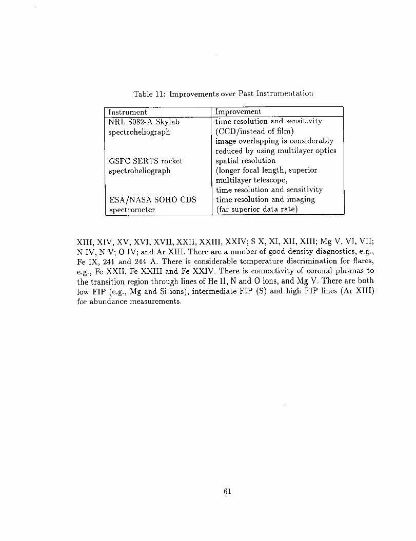
Table 11: Improvements over Past Instrumentation
Instrument Improvement
NRL S082-A Skylab
spectroheliograph
GSFC SERTS rocket
spectroheliograph
ESA/NASA SOHO CDS
spectrometer
time resolution and sensitivity
(CCD/instead of film)
image overlapping is considerably
reduced by using multilayer optics
spatial resolution
(longer focal length, superior
multilayer telescope,
time resolution and sensitivity
time resolution and imaging
(far superior data rate)
XIII, XIV, XV, XVI, XVII, XXII, XXIII, XXIV; S X, XI, XII, XIII; Mg V, VI, VII;
N IV, N V; O IV; and Ar XIII. There are a number of good density diagnostics, e.g.,
Fe IX, 241 and 244 A. There is considerable temperature discrimination for flares,
e.g., Fe XXII, Fe XXIII and Fe XXIV. There is connectivity of coronal plasmas to
the transition region through lines of He II, N and 0 ions, and Mg V. There are both
low FIP (e.g., Mg and Si ions), intermediate FIP (S) and high FIP lines (Ar XIII)
for abundance measurements.
61

APPENDICES
A The Solar-B Spacecraft
A.1 Orbit
Solar-B will be launched by an M-5 rocket into a 600-km circular polar Sun-synchronous
orbit at 97.79 degrees inclination. Such an orbit has several advantages:
• Continuous solar viewing for approximately eight months, followed by four
months with short (up to 20 min) eclipses.
• The long intervals of continuous sunlight greatly simplify the thermal design of
the spacecraft.
Spacecraft motion projected in the solar direction, responsible for Doppler errors
in radial velocity measurements, varies slowly (less than +0.1 m/_/s) and over
a relatively small amplitude (less than -t-100 m_).
The Sun-synchronous orbit includes passages through the auroral zones, as well as
the South Atlantic Anomaly. It also exposes the spacecraft to infrequent but intense
solar particle events. Table 12 summarizes the properties of the proposed Solar-B
orbit in comparison with a standard low-inclination orbit.
To achieve and maintain the proper orbit, the Solar-B spacecraft will require a
propulsion system (Hydrazine thrusters).
A.2 Satellite Structure
The principal constraints on spacecraft structural design are
• The optical telescope/magnetograph is bulky and heavy (a package about 1 m
diameter, 3.5 m length, and 200 kg mass) and constitutes the central structureof the satellite.
• The optical system has to be well-maintained thermally, considering the solar
input, in order to achieve the diffraction limit of 0.2".
In view of the bulk and precision of the optical telescope/magnetograph instru-
ment (see Table 13), it will dominate the structural and thermal design of the space-
craft. The baseline design concept consists of a cylindrical thrust tube, 1 m diameter
x 2.2 m length, thermally controlled by heat pipes, as shown in Figure 24. The
thrust tube will also serve as an optical bench for the X-ray and XUV instruments
(externally), and will also permit mounting of spacecraft common systems.
62
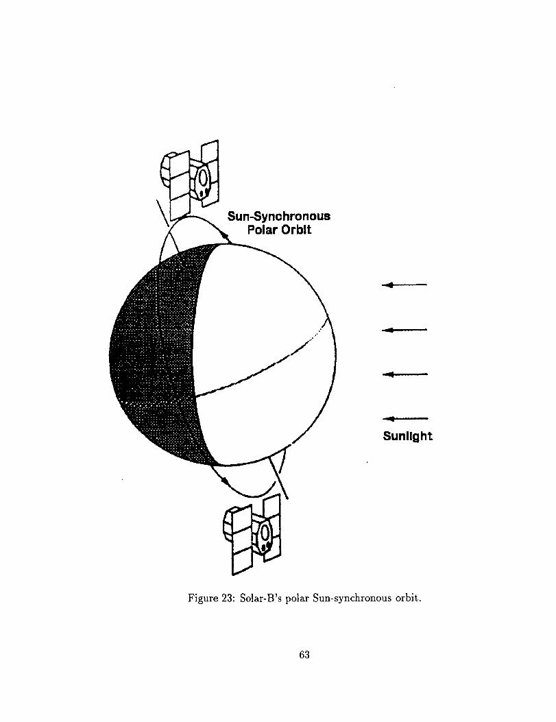
Sun-SynohronousPolar Orbit
Sunlight
Figure 23: Solar-B's polar Sun-synchronous orbit.
63

°1 i
: 2000
59_0
1
za0o
m
\RCS Tank
\ Solar Paddle
Bus Module
500 x 1800
$5_0
i
Optical Telescope
Thrust Tube
X-Ray
Telescope
\
XUV SpectTograph
Bus Module
. $1000 r
Figure 24: Solar-B spacecraft layout and basic dimensions.
64

Table 12: Orbit Comparison
Orbit type Sun-synchronous Low-inclination
Observations
Doppler shifts
Power/thermal
Spacecraft
mass
Orbit
injection
High-energyParticles
8 months/year, no eclipse
Lower; zero twice a yearEasier
850 Kg
More difficult
South Atlantic AnomalyAuroral zones
Solar particles
Eclipse duration
40 minutes per orbit
250 m_ p-p (5000 A)
More difficult
1200 Kg
Easier
South Atlantic Anomaly
A.3 Attitude Control
The Solar-B attitude control systems envisions the use of the spacecraft itself for
coarse pointing, plus internal image motion compensation for small angles and high
frequencies within the observing instruments as needed. The spacecraft will use a
combination of magnetic torquers, gyros, momentum wheels, and possibly momentum
adjustment devices to control torques due to internal motions, for example from filterwheels.
Table 14 compares the pointing stability envisioned for Solar-B in comparison
with that achieved by Yohkoh. The X and Y axes are orthogonal to the Z-axis, in the
Sun-Earth direction; Y is aligned with the solar rotational pole. Table 15 gives the
requirements for alignment of the optical telescope, to be achieved by image motion
compensation within the instrument itself.
The optical telescope/magnetograph must be able to position its small field of
view anywhere on the solar disk, so that simple Sun-center pointing is not sufficient.
The field of view may need to track the solar rotation, which is as large as 2 km/s
(0.003"/sec) at disk center and is a function (the differential rotation) of solar latitude.
To accomplish this a set of on-board reference tables may be used to select a suitable
spacecraft pointing motion as a function of observing position on the solar disk.
65

Table 13: Weight and Power Breakdown
Spacecraftcomponents Weight (kg) Power (W)Dual thruster systemAttitude control systemPower systemTelemetry systemCommand/data processorsystemThermal control systemInsulationSupport structureCable harnessLaunch systems
16994781113524150105
20352034120
Subtotal 559 382
Payload componentsOptical telescopeX-ray telescopeXUV spectrographParticle monitorMission data processor& recorder
2003060610
2020205t0
Subtotal 310 75
Total 874 457 ]
Table 14: Pointing precision(peak-to-peakerror)
Short-term stability
Long-term stability
Absolute pointing
Solar-B YohkohX,Y 0.2"/secZ 30"/secX,Y 0.4"/minZ 1.5'/rainX,Y < 1'Z < 2'
1.2"/sec5'/sec7"/min7'/min<6'<10'
66

Table 15: Alignment precision for optical telescope (peak-to-peak error) 1
lO-sec interval X,Y 0.02"/10 sec
Z 2 30"/10 sec
1-minute interval X,Y 0.4"/min
Z 2 1.5'/min
One-hour interval X,Y 2'r/hour
Z 1
1 To be achieved by a combination of spacecraft motion and tilt-mirror adjustments within the
optical telescope.2 Not achievable by measurements within the optical instrument, thus a spacecraft requirement.
3 See Table 15.
A.4 Data Storage and Transmission
On-board processing
The Solar-B instruments will be capable of generating as much as 8 Gbit per orbit.
Even to transmit 10 minutes of observational material would require a downlink rate
of 13 Mbps. To handle this problem Solar-B will have hardware implementations of
both lossless (DPCM) and lossy (JPEG) compression algorithms. Gate array chips
have been developed for this purpose. The Solar-B data system envisions
• Data generation rate, about 500 kbps
• On-board recorder (one orbit's data), about 3 Gb
• Downlink rate, about 5 Mbps
The currently-available HCMOS technology is adequate for the on-board data
storage system.
Data transmission
The ISAS programs ASTRO-E and ASTRO-F, which precede Solar-B, will require
few-Mbps downlink capability (S-band and X-band at KSC). These systems are close
to satisfying the Solar-B requirements. The availability of DSN sites for additional
telemetry made many Yohkoh results possible, and the Solar-B program would like
also to be able to use DSN. At present, however, the maximum available rate (via
convolution coding) is 2.2 Mbps.
67

B Projected Cost
FY
New
Start
AO Selection RR PDR CDR PM FM
V V V V V VL=unch
V
CY
• Phase B
• Proto Model
D eve/opment
• F IJght M o¢ieJ
D eveJopment
• Test Phase Optics
• "fesl Phase AJJ Systems
• M O& DA Phase
_The total reflects a cost cap established for a launch in 02.
Figure 25: Projected cost outline for the U. S. contribution to the Solar-B mission,
time phased with respect to the major milestones of the ISAS Solar-B program.
68