The Sliding DFT

The standard methodfor spectrum analysisin digital signal pro-cessing (DSP) is thediscrete Fourier

transform (DFT), typically imple-mented using a fast Fourier transform(FFT) algorithm. However, there areapplications that require spectrumanalysis only over a subset of the Ncenter frequencies of an N-point DFT.A popular, as well as efficient, tech-nique for computing sparse DFT re-sults is the Goertzel algorithm thatcomputes a single complex DFT spec-tral bin value for every N input timesamples. This article describes a slidingDFT process whose spectral bin out-put rate is equal to the input data rate,on a sample-by-sample basis, with theadvantage that it requires fewer com-putations than the Goertzel algorithmfor real-time spectral analysis. In appli-cations where a new DFT output spec-trum is desired every sample, or everyfew samples, the sliding DFT iscomputationally simpler than the tra-ditional radix-2 FFT. We’ll start oursliding DFT discussion by providing abrief review of the Goertzel algorithmand use its behavior as a yardstick toevaluate the performance of the slidingDFT technique. Following that, wewill examine stability issues regardingthe sliding DFT implementation as

well as review the process of fre-quency-domain convolution to ac-complish time-domain windowing.Finally, a modified sliding DFT struc-ture is proposed that provides im-proved computational efficiency.

Goertzel AlgorithmThe Goertzel algorithm, used indual-tone multifrequency decodingand phase-shift keying/frequency-shiftkeying modem implementations, iscommonly used to compute DFTspectra [1]-[4]. The algorithm is im-plemented in the form of a second-or-der infinite impulse response (IIR)filter as shown in Figure 1. This filtercomputes a single DFT output (thekth bin of an N-point DFT) definedby

X k x n e j nk N

n

N

( ) ( ) /= −

=

−

∑ 2

0

1π .

(1)

The filter’s y n( ) output is equal tothe DFT output frequency coeffi-cient, X k( ), at the time index n N= .For emphasis, we remind the readerthat the filter’s y n( ) output is notequal to X k( ) at any time index whenn N≠ . The frequency-domain indexk i s an integer in the range0 1≤ ≤ −k N . The derivation of this

filter’s structure is readily available inthe literature [5]-[7].

The z-domain transfer function ofthe Goertzel filter is

H z

e zk N z z

G

j k N

( )

cos( / )

/

= −− +

− −

− −

11 2 2

2 1

1 2

π

π

(2)

with a single z-domain zero located atz e j k N= − 2 π / and conjugate poles atz e j k N= ± 2 π / as shown in Figure 2(a).The pole/zero pair at z e j k N= − 2 π / can-cels each other. The frequency magni-tude response, provided in Figure2(b), shows resonance centered at anormalized frequency of 2πk N/ , cor-responding to a cyclic frequencyk f Ns⋅ / Hz (where f s is the signalsample rate).

While the Goertzel algorithm isderived from the standard DFT equa-tion, it’s important to realize that thefilter’s frequency magnitude responseis not the sin( )/( )x x -like response of asingle-bin DFT. The Goertzel filter isa complex resonator having an infi-nite-length unit impulse response,h n e j nk N( ) /= 2 π , and that’s why itsmagnitude response is so narrow.The time-domain difference equa-tions for the Goertzel filter are

v n k N v nv n x n

( ) cos( / ) ( )( ) ( )

= −− − +2 2 1

2π

(3a)

y n v n e v nj k N( ) ( ) ( )./= − −− 2 1π (3b)

An advantage of the Goertzel filterin calculating an N-point X k( ) DFT

74 IEEE SIGNAL PROCESSING MAGAZINE MARCH 20031053-5888/03/$17.00©2003IEEE

Eric Jacobsen and Richard Lyons

“DSP Tips and Tricks” introduces practical tips and tricks of design and imple-mentation of signal processing algorithms so that you may be able to incor-porate them into your designs. We welcome readers who enjoy reading thiscolumn to submit their contributions. Please contact Associate Editor Rick Ly-ons at ricklyon@onemain.com.

bin is that (3a) is implemented Ntimes while (3b), the feed forwardpath in Figure 1, need only be com-puted once after the arrival of the Nthinput sample. Thus for real x n( ) thefilter requires N + 2 real multipliesand 2 1N + real adds to compute anN-point X k( ). However, when mod-eling the Goertzel filter if the time in-dex begins at n = 0, the filter mustprocess N + 1 time samples withx N( ) = 0 to compute X k( ). Now let’slook at the sliding DFT process.

Sliding DFTThe sliding DFT (SDFT) algorithmperforms an N-point DFT on timesamples within a sliding-window asshown in Figure 3. In this examplethe SDFT initially computes the DFTof the N = 16 time samples in Figure3(a). The time window is then ad-vanced one sample, as in Figure 3(b),and a new N-point DFT is calculated.The value of this process is that eachnew DFT is efficiently computed di-rectly from the results of the previousDFT. The incremental advance of thetime window for each output compu-tation is what leads to the name slid-ing DFT or sliding-window DFT.

The principle used for the SDFT isknown as the DFT shifting theoremor the circular shift property [8]. Itstates that if the DFT of a windowed(finite-length) time-domain se-quence is X k( ), then the DFT of thatsequence, circularly shifted by onesample, is X k e j k N( ) /2 π . Thus the spec-tral components of a shifted time se-quence are the original (unshifted)spectral components multiplied bye j k N2 π / , where k is the DFT bin of in-terest. We express this process by

S n S n ex n N x n

k kj k N( ) ( )

( ) ( )

/= −− − +

1 2 π

(4)

where S nk ( ) is the new spectral com-ponent and S nk ( )− 1 is the previousspectral component. The subscript k

MARCH 2003 IEEE SIGNAL PROCESSING MAGAZINE 75

▲ 1. IIR filter implementation of the Goertzel algorithm.

▲ 2. Goertzel filter: (a) z-domain pole/zero locations and (b) frequency magnitude re-sponse.

▲ 3. Signal windowing for two 16-point DFTs: (a) data samples in the first computationand (b) second computation samples.

reminds us that the spectra are thoseassociated with the kth DFT bin.

Equation (4), whose derivation isprovided in the Appendix, reveals thevalue of this process in computingreal-time spectra. We calculate S nk ( )by phase shifting the previousS nk ( )− 1 components, subtract thex n N( )− sample, and add the currentx n( ) sample. Thus the SDFT requiresonly one complex multiply and tworeal adds per output sample. The com-putational complexity of each succes-sive N-point output is then O( )N forthe sliding DFT compared to O( )N 2

for the DFT and O[ log ( )]N N2 forthe FFT. Unlike the DFT or FFT,however, due to its recursive naturethe sliding DFT output must be com-puted for each new input sample. If anew N-point DFT output is requiredonly every N inputs, the sliding DFTrequires O( )N 2 computations and isequivalent to the DFT. When outputcomputations are required every M in-

put samples, and M is less thanlog ( )2 N , the sliding DFT can becomputationally superior to tradi-tional FFT implementations evenwhen all N DFT outputs are required.

Equation (4) leads to the sin-gle-bin SDFT filter structure shownin Figure 4.

The single-bin SDFT algorithm isimplemented as an IIR filter with acomb filter followed by a complexresonator [9]. (If you want to com-pute all N DFT spectral components,N resonators with k = 0 to N − 1 willbe needed, all driven by a single combfilter.) The comb filter delay of Nsamples forces the filter’s transient re-sponse to be N − 1samples in length,so the output will not reach steadystate until theS Nk ( )sample. In practi-cal applications the algorithm can beinitialized with zero input and zerooutput. The output will not be valid,or equivalent to (1)’s X k( ), until N in-put samples have been processed. The

z-domain transfer function for the kthbin of the sliding DFT filter is

H zz

e z

N

j k NSDFT ( )( )

/=

−−

−

−

11 2 1π

.(5)

This complex filter has N zerosequally spaced around the z-domain’sunit circle, due to the N-delay combfilter, as well as a single pole cancelingthe zero at z e j k N= 2 π / . The SDFT fil-ter’s complex unit impulse responseh n( ) and pole/zero locations areshown in Figure 5 for the examplewhere k = 2 and N = 20.

Because of the comb subfilter, theSDFT filter’s complex sinusoidal unitimpulse response is finite in length,truncated in time to N samples, andthat property makes the frequencymagnitude response of the SDFT fil-ter identical to the sin( )/sin( )Nx x re-sponse of a single DFT bin centeredat a normalized frequency of 2πk N/ .

One of the attributes of the SDFTis that once an S nk ( )− 1 is obtained,the number of computations to calcu-late S nk ( ) is fixed and independent ofN. A computational workload com-parison between the Goertzel andSDFT filters is provided later in thisarticle. Unlike the radix-2 FFT, theSDFT’s N can be any positive integergiving us greater flexibility to tune theSDFT’s center frequency by defininginteger k such that k N f fi s= ⋅ / ,when f i is a frequency of interest inhertz. In addition, the SDFT does notrequire bit-reversal processing as doesthe FFT. Like Goertzel, the SDFT isespecially efficient for narrowbandspectrum analysis.

For completeness, we mentionthat a radix-2 sliding FFT techniqueexists for computing all N bins of X k( )in (1) [10], [11]. This method iscomputationally attractive because itrequires only N complex multiplies toupdate the N-point FFT for all Nbins; however, it requires 3N mem-ory locations (2N for data and N fortwiddle coefficients). Unlike the

76 IEEE SIGNAL PROCESSING MAGAZINE MARCH 2003

x n( )

z −N

−1 ej k N2 /π

S nk( 1)−

S nk( )+ +

z −1

▲ 4. Single-bin sliding DFT filter structure.

1

0

−10 2 4 6 8 10 12 14 16 18 20

Real [ ( )]h n

Imag

inar

yP

art

1

0.5

0

−0.5

−1

−1 0 1Real Part

2 /πk N

k = 2N = 20

1

0

−10 2 4 6 8 10 12 14 16 18 20

Imag [ ( )]h n

(a) (b)

▲ 5. Sliding DFT characteristics for k = 2 and N = 20: (a) impulse response and (b)pole/zero locations.

SDFT, the radix-2 sliding FFTscheme requires address bit-reversalprocessing and restricts N to be an in-teger power of two.

SDFT StabilityThe SDFT filter is only marginallystable because its pole resides on thez-domain’s unit circle. If filter coeffi-cient numerical rounding error is notsevere, the SDFT is bounded-input,bounded-output stable. Filter insta-bility can be a problem, however, ifnumerical coefficient roundingcauses the filter’s pole to move out-side the unit circle. We can use adamping factor r to force the pole tobe at a radius of r inside the unit circleand guarantee stability using a trans-fer function of

H zr z

re zgs

N N

j k NSDFT, ( )( )

/=

−−

−

−

11 2 1π (6)

with the subscript gs meaning guaran-teed-stable. The stabilized feed-for-ward and feedback coefficientsbecome −r N and re j k N2 π / , respec-tively. The difference equation for thestable SDFT filter becomes

S n S n re

x n N r x nk gs k gs

j k N

N

, ,/( ) ( )

( ) ( )

= −

− − +

1 2 π

(7)

with the stabilized-filter structureshown in Figure 6.

Using a damping factor as in Fig-ure 6 guarantees stability, but theS nk ( ) output, defined by

X k x n rerj nk N

n

N

<−

=

−

= ⋅∑12

0

1

( ) ( ) /π

(8)

is no longer exactly equal to the kth binof an N-point DFT in (1). While theerror is reduced by making r very closeto (but less than) unity, a scheme doesexist for eliminating that error com-pletely once every N output samples atthe expense of additional conditional

logic operations [12]. Determining ifthe damping factor r is necessary for aparticular SDFT application requirescareful empirical investigation.

Another stabilization methodworth consideration is decrementingthe largest component (either real orimaginary) of the filter’s e j k N2 π / feed-back coefficient by one least significantbit. This technique can be applied se-lectively to problematic output binsand is effective in combating instabil-ity due to rounding errors which resultin finite-precision e j k N2 π / coefficientshaving magnitudes greater than unity.

Like the DFT, the SDFT’s outputis proportional to N, so in fixed-pointbinary implementations the designermust allocate sufficiently wide regis-ters to hold the computed results.

Time-Domain Windowingin the Frequency DomainThe spectral leakage of the SDFT canbe reduced by the standard concept ofwindowing the x n( ) input time sam-

ples. However, windowing by time-domain multiplication would compro-mise the computational simplicity ofthe SDFT. Alternatively, we can imple-ment a time-domain window by meansof frequency-domain convolution.

Spectral leakage reduction per-formed in the frequency domain is ac-complished by convolving adjacentS nk ( ) values with the DFT of awindow function. For example, theDFT of a Hanning window com-prises only three nonzero values,−0.25, 0.5, and −0.25. As such we cancompute a Hanning-windowedS nk ( ),the kth DFT bin, with a three-pointconvolution using

Hanning-windowedS n S n S n

S nk k k

k

( ) . ( ) . ( )

. ( ).

= − ⋅ + ⋅

− ⋅−

+

025 05

0251

1 (9)

Figure 7 shows this process wherethe comb filter stage need only be im-plemented once. Thus a Hanningwindow can be implemented by bi-nary right shifts (assuming integer

MARCH 2003 IEEE SIGNAL PROCESSING MAGAZINE 77

x n( )

z −N

+ +S nk( )

z −1

−r N rej k N2 /π

S nk( 1)−

▲ 6. Guaranteed-stable sliding DFT filter structure.

x n( )

z −N

Resonator1k−

Resonatork

Resonator1k+

+

−1

S nk−1( )

S nk( )

S nk+1( )

−0.25

0.5

−0.25

WindowedS ( ) Outputk n

+

▲ 7. Three-resonator structure to compute three SDFT bin results and a three-point con-volution.

arithmetic) and two complex adds foreach SDFT bin, making the Hanningwindow attractive in ASIC andFPGA implementations where sin-gle-cycle hardware multiplies arecostly. If a gain of four is acceptable,then only one left shift two complexadds are required using

Hanning-windowedS n S n S n S nk k k k( ) ( ) ( ) ( ).= − + ⋅ −− +1 12

(10)

The Hanning window is a memberof a category called cos ( )α x windowfunctions [13], [14]. These functionsare also known as generalized cosinewindows because their N-pointtime-domain samples are defined as

w n a mn Nmm

m

( ) ( ) cos( / )= −=

−

∑ 1 20

1

πα

(11)

where n N= −0 1 2 1, , , ... , , and theinteger α specifies the number ofterms in the window’s time function.These window functions are attrac-tive for frequency domain convolu-tion because their DFTs contain onlya few nonzero samples. The fre-quency domain vectors of variouscos ( )α x window functions follow theform ( / ) ( , , , , )1 2 22 1 0 1 2⋅ − −a a a a a ,with a few examples presented in Ta-ble 1. Additional cos ( )α x windowfunctions are described in the litera-ture [14].

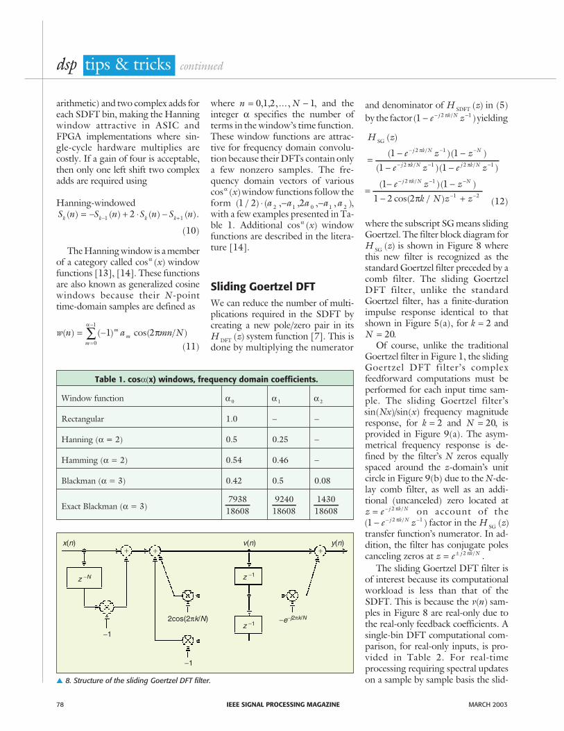
Sliding Goertzel DFTWe can reduce the number of multi-plications required in the SDFT bycreating a new pole/zero pair in itsH zDFT ( ) system function [7]. This isdone by multiplying the numerator

and denominator of H zSDFT ( ) in (5)by the factor( )/1 2 1− − −e zj k Nπ yielding

H z

e z ze z e

j k N N

j k N j

SG ( )

( )( )( )(

/

/=

− −− −

− − −

− −

1 11 1

2 1

2 1 2

π

π π

π

π

k N

j k N N

z

e z zk N z z

/

/

)

( )( )cos( / )

−

− − −

− −=

− −− +

1

2 1

1

1 11 2 2 2

(12)

where the subscript SG means slidingGoertzel. The filter block diagram forH zSG ( ) is shown in Figure 8 wherethis new filter is recognized as thestandard Goertzel filter preceded by acomb filter. The sliding GoertzelDFT filter, unlike the standardGoertzel filter, has a finite-durationimpulse response identical to thatshown in Figure 5(a), for k = 2 andN = 20.

Of course, unlike the traditionalGoertzel filter in Figure 1, the slidingGoertzel DFT filter’s complexfeedforward computations must beperformed for each input time sam-ple. The sliding Goertzel filter’ssin( )/sin( )Nx x frequency magnituderesponse, for k = 2 and N = 20, isprovided in Figure 9(a). The asym-metrical frequency response is de-fined by the filter’s N zeros equallyspaced around the z-domain’s unitcircle in Figure 9(b) due to the N-de-lay comb filter, as well as an addi-tional (uncanceled) zero located atz e j k N= − 2 π / on account of the( )/1 2 1− − −e zj k Nπ factor in the H zSG ( )transfer function’s numerator. In ad-dition, the filter has conjugate polescanceling zeros at z e j k N= ± 2 π / .

The sliding Goertzel DFT filter isof interest because its computationalworkload is less than that of theSDFT. This is because the v n( ) sam-ples in Figure 8 are real-only due tothe real-only feedback coefficients. Asingle-bin DFT computational com-parison, for real-only inputs, is pro-vided in Table 2. For real-timeprocessing requiring spectral updateson a sample by sample basis the slid-

78 IEEE SIGNAL PROCESSING MAGAZINE MARCH 2003

Table 1. cos x) windows, frequency domain coefficients.

Window function α 0 α 1 α 2

Rectangular 1.0 − −

Hanning (α = 2) 0.5 0.25 −

Hamming (α = 2) 0.54 0.46 −

Blackman (α = 3) 0.42 0.5 0.08

Exact Blackman (α = 3)7938

186089240

186081430

18608

x n( )

z −N

+

−1

+

−1

z −12cos(2 / )πk N −e− πj k N2 /

y n( )v n( )

z −1

+

▲ 8. Structure of the sliding Goertzel DFT filter.

ing Goertzel method requires fewermultiplies than either the SDFT orthe traditional Goertzel algorithm.

SummaryThe sliding DFT process for spectrumanalysis was presented and shown to bemore efficient than the popularGoertzel algorithm for sample-by-sam-ple DFT bin computations. The slidingDFT provides computational advan-tages over the traditional DFT or FFTfor many applications requiring succes-sive output calculations, especiallywhen only a subset of the DFT outputbins are required. Methods for outputstabilization as well as time-domaindata windowing by means of fre-quency- domain convolution were alsodiscussed. A modified sliding DFT al-gorithm, called the sliding GoertzelDFT, was proposed to further reducecomputational workload.

Eric Jacobsen is minister of algorithms atIntel. He currently leads the AdvancedOFDM wireless research effort withinIntel Labs and has interests in channelmodeling, efficient algorithms, syn-chronization, coding, adaptive tech-niques, and other aspects of wirelesscommunication systems. He has devel-oped efficient hardware and softwareimplementation techniques for signalprocessing in radar, imaging, satellite,and communications systems. With anM.S.E.E. from South Dakota Schoolof Mines and Technology, he is a mem-ber of the IEEE and the Eta Kappa Nuhonor society and occasionally roadraces a 1995 Taurus SHO.

Richard Lyons is a consulting systemsengineer and lecturer with Besser As-sociates in Mt. View, California. Hehas been the lead hardware engineerfor numerous multimillion dollar sig-nal processing systems for both theNational Security Agency (NSA) andTRW Inc. and has taught at the Uni-versity of California Santa Cruz Ex-tension. He is an associate editor for

IEEE Signal Processing Magazine andauthor of Understanding Digital Sig-nal Processing (Prentice-Hall, 1997).He is a member of the IEEE and theEta Kappa Nu honor society andrides a 1981 Harley Davidson.

References[1] M. Felder, J. Mason, and B. Evans, “Efficient dual-

tone multi-frequency detection using the non-uni-form discrete Fourier transform,” IEEE Signal Pro-cessing Lett., vol. 5, pp. 160-163, July 1998.

[2] Using the ADSP-2100 Family, vol. 1. Norwood,MA: Analog Devices, 1995, chap. 14 [Online].Available: http://www.analog.com/Ana-log_Root/static/library/dspManuals/Us-ing_ADSP-2100_Vol1_books.html

[3] S. Gay, J. Hartung, and G. Smith, “Algorithmsfor multi-channel DTMF detection for theWERDSP32 family,” in Proc. Int. Conf. ASSP,1989, pp. 1134-1137.

[4] K. Banks, “The Goertzel algorithm,” EmbeddedSyst. Programming Mag., pp. 34-42, Sept. 2002.

[5] G. Goertzel, “An algorithm for the evaluation offinite trigonometric series,” American Math.Month., vol. 65, pp. 34-35, 1958.

[6] J. Proakis and D. Manolakis, Digital Signal Pro-cessing-Principles, Algorithms, and Applications,3rd ed. Upper Saddle River, NJ: Prentice Hall,1996, pp. 480-481.

[7] A. Oppenheim, R. Schafer, and J. Buck, Dis-crete-Time Signal Processing, 2nd ed. Upper Sad-dle River, NJ: Prentice Hall, 1996, pp. 633-634.

[8] T. Springer, “Sliding FFT computes frequencyspectra in real time,” EDN Mag., pp. 161-170,Sept. 29, 1988.

[9] L. Rabiner and B. Gold, Theory and Applicationof Digital Signal Processing. Upper Saddle River,NJ: Prentice Hall, 1975, pp. 382-383.

[10] B. Farhang-Boroujeny and Y. Lim, “A com-ment on the computational complexity of slid-ing FFT,” IEEE Trans. Circuits Syst. II, vol. 39,no. 12, pp. 875-876, Dec. 1992.

[11] B. Farhang-Boroujeny and S. Gazor, “General-ized sliding FFT and its application to imple-mentation of block LMS adaptive filters,” IEEETrans. Signal Processing, vol. 42, no. 3, pp.532-538, Mar. 1994.

[12] S. Douglas and J. Soh, “A numerically stablesliding-window estimator and its application toadaptive filters,” in Proc. 31st Annual AsilomarConf. on Signals, Systems, and Computers, PacificGrove, CA, vol. 1, Nov. 1997, pp. 111-115.

MARCH 2003 IEEE SIGNAL PROCESSING MAGAZINE 79

Table 2. Single-bin DFT comparison.

Single S nk( ) ComputationNext S nk( )+ 1Computation

RealMultiplies Real Adds

RealMultiplies Real Adds

DFT 2N 2N 2N 2N

Standard Goertzel N + 2 2N + 1 N + 2 2N + 1

Sliding DFT 4N 4N 4 4

Sliding Goertzel DFT N + 2 3N + 1 3 4Im

agin

ary

Par

t

1

0.5

0

−0.5

−1

−1 0 1

Real Part

2 /πk N

k = 2N = 20

(b)

dB

0

−5

−10

−15

−20

−25

−300

k = 2N = 20

fs/4 fs/2 3 /4fs fsFrequency

(a)

TwoZeros

▲ 9. Sliding Goertzel filter for N = 20 and k = 2: (a) frequency magnitude response and(b) z-domain pole/zero locations.

[13] F. Harris, “On the use of windows for harmonicanalysis with the discrete Fourier transform,”Proc. IEEE, vol. 66, pp. 51-84, Jan. 1978.

[14] A. Nuttall, “Some windows with very goodsidelobe behavior,” IEEE Trans. Acoust., Speech,Signal Processing,, vol. 29, pp. 84-91, Feb. 1981.

AppendixThe derivation of the SDFT time-do-main expression is straightforward byexample. We start by using the princi-ples of the z-transform and write ageneralized z-domain spectrum of afour-point time-domain sequencex n( ), where n = 0 1 3, , ... , , evaluated atz zo= as

S x x z

x z x zz o

o o

o( ) ( ) ( )

( ) ( ) .

0 3 2

1 02 3

= +

+ + (A1)

Likewise we could compute aspectrum of the four x n( )+ 1 timesamples as

S x x z

x z x zz o

o o

o( ) ( ) ( )

( ) ( ) .

1 4 3

2 12 3

= +

+ + (A2)

If we multiply Sz o( )0 by zo we have

S z x z x z

x z x zz o o o

o o

o( ) ( ) ( )

( ) ( ) .

0 3 2

1 0

2

3 4

= +

+ + (A3)

Comparing (A2) and (A3) we canrewrite (A2) as

S S z x z xz z o oo o( ) ( ) ( ) ( )1 0 0 44= − + .

(A4)

Thus we can use Sz o( )0 to com-

puteSz o( )1 . Moreover we can express

the spectrum of the four x n( )+ 2samples as

S S z x z xz z o oo o( ) ( ) ( ) ( )2 1 1 54= − + .

(A5)

In the general case, the qth N-pointspectrum can be expressed as

S q S q z x q zx q N

z z o oN

o o( ) ( ) ( )

( ).= − − −

+ + −1 1

1 (A6)

Here’s the payoff for our efforts. Ifwe let z eo

j k N= 2 π / , a point on the unitcircle, the (A6) z-transform expressionbecomes the desired time-domain ex-pression for the sliding DFT as

S q S q e

x q ex

e e

j k N

j kN N

j k N j k N2 2 1

1

2

2

π π

π

π

/ /( ) ( )

( )(

/

/

= −

− −+ q N

S q e

x q x q Ne

j k Nj k N

+ −

= −

− − + + −

1

1

1 12

2

)

( )

( ) ( )./

/π

π

(A7)

Because the angle of e j k N2 π / is aninteger multiple of2π/N, (A7) is seenmerely as the qth single-bin DFT,X k( ), of x n( ) for the normalized fre-quency of 2πk N/ radians, wherek N= −0 1 2 1, , , ... , . We now have anexpression for the sliding DFT. How-ever, to turn that expression into a fil-ter dif ference equation we’recompelled to modify the indices of

(A7) to make them compatible withcausal filters. With no loss in general-ity, using the following substitutions

S n S q

S n S q

x n x q N

k e

k e

j k N

j k N

( ) ( ),

( ) ( ),

( ) (

/

/

=

− = −

= +

2

21 1π

π

−− = −

11

),( ) ( ),x n N x q (A8)

we can rewrite (A7) in a time-domainform for the causal recursive filter

S n S n ex n N x n

k kj k N( ) ( )

( ) ( ).

/= −− − +

1 2 π

(A9)

The subscript k reminds us that thefilter output is associated with thekth DFT bin. The z-domain transferfunction for the kth bin of the slidingDFT filter is

H zz

e z

N

j k NSDFT ( )( )

/=

−−

−

−

11 2 1π

.(A10)

80 IEEE SIGNAL PROCESSING MAGAZINE MARCH 2003