the skorokhod embedding problem and its offspring · j. obl ´oj/skorokhod embedding problem 326...

arX

iv:m

ath/

0401

114v

4 [

mat

h.PR

] 1

0 N

ov 2

005

Probability Surveys

Vol. 1 (2004) 321–392ISSN: 1549-5787DOI: 10.1214/154957804100000060

The Skorokhod embedding problem and

its offspring∗

Jan Ob loj†

Laboratoire de Probabilites et Modeles Aleatoires, Universite Paris 64 pl. Jussieu, Boite 188, 75252 Paris Cedex 05, France.

Department of Mathematics, Warsaw Universityul. Banacha 2, 02-097 Warszawa, Poland.

e-mail: [email protected]

Abstract: This is a survey about the Skorokhod embedding problem. Itpresents all known solutions together with their properties and some appli-cations. Some of the solutions are just described, while others are studiedin detail and their proofs are presented. A certain unification of proofs,based on one-dimensional potential theory, is made. Some new facts whichappeared in a natural way when different solutions were cross-examined,are reported. Azema and Yor’s and Root’s solutions are studied extensively.A possible use of the latter is suggested together with a conjecture.

Keywords and phrases: Skorokhod embedding problem, Chacon-Walshembedding, Azema-Yor embedding, Root embedding, stopping times, opti-mal stopping, one-dimensional potential theory.AMS 2000 subject classifications: Primary 60G40, 60G44; Secondary60J25, 60J45.

Received March 2004.

∗This is an original survey paper.†Work partially supported by French government (scholarship No 20022708) and Polish

Academy of Science.

321

http://arXiv.org/abs/math/0401114v4

http://stat-www.berkeley.edu/users/prsurvey

http://dx.doi.org/10.1214/154957804100000060

mailto:[email protected]

J. Ob loj/Skorokhod embedding problem 322

Contents

1 Introduction 324

2 The problem and the methodology 3262.1 Preliminaries . . . . . . . . . . . . . . . . . . . . . . . . . . . . . 3272.2 On potential theory . . . . . . . . . . . . . . . . . . . . . . . . . 3282.3 The Problem . . . . . . . . . . . . . . . . . . . . . . . . . . . . . 330

3 A guided tour through the different solutions 3313.1 Skorokhod (1961) . . . . . . . . . . . . . . . . . . . . . . . . . . . 3313.2 Dubins (1968) . . . . . . . . . . . . . . . . . . . . . . . . . . . . . 3323.3 Root (1968) . . . . . . . . . . . . . . . . . . . . . . . . . . . . . . 3333.4 Hall (1968) . . . . . . . . . . . . . . . . . . . . . . . . . . . . . . 3333.5 Rost (1971) . . . . . . . . . . . . . . . . . . . . . . . . . . . . . . 3343.6 Monroe (1972) . . . . . . . . . . . . . . . . . . . . . . . . . . . . 3373.7 Heath (1974) . . . . . . . . . . . . . . . . . . . . . . . . . . . . . 3373.8 Chacon and Walsh (1974-1976) . . . . . . . . . . . . . . . . . . . 3373.9 Azema-Yor (1979) . . . . . . . . . . . . . . . . . . . . . . . . . . 3393.10 Falkner (1980) . . . . . . . . . . . . . . . . . . . . . . . . . . . . 3393.11 Bass (1983) . . . . . . . . . . . . . . . . . . . . . . . . . . . . . . 3393.12 Vallois (1983) . . . . . . . . . . . . . . . . . . . . . . . . . . . . . 3403.13 Perkins (1985) . . . . . . . . . . . . . . . . . . . . . . . . . . . . 3413.14 Jacka (1988) . . . . . . . . . . . . . . . . . . . . . . . . . . . . . . 3413.15 Bertoin and Le Jan (1993) . . . . . . . . . . . . . . . . . . . . . . 3413.16 Vallois (1994) . . . . . . . . . . . . . . . . . . . . . . . . . . . . . 3423.17 Falkner, Grandits, Pedersen and Peskir (2000 - 2002) . . . . . . . 3433.18 Roynette, Vallois and Yor (2002) . . . . . . . . . . . . . . . . . . 3443.19 Hambly, Kersting and Kyprianou (2002) . . . . . . . . . . . . . . 3443.20 Cox and Hobson (2004) . . . . . . . . . . . . . . . . . . . . . . . 3453.21 Ob loj and Yor (2004) . . . . . . . . . . . . . . . . . . . . . . . . . 345

4 Embedding measures with finite support 3484.1 Continuous local martingale setup . . . . . . . . . . . . . . . . . 3484.2 Random walk setup . . . . . . . . . . . . . . . . . . . . . . . . . 349

5 Around the Azema-Yor solution 3505.1 An even simpler proof of the Azema-Yor formula . . . . . . . . . 3515.2 Nontrivial initial laws . . . . . . . . . . . . . . . . . . . . . . . . 3535.3 Minimizing the minimum - the reversed AY solution . . . . . . . 3555.4 Martingale theory arguments . . . . . . . . . . . . . . . . . . . . 3565.5 Some properties . . . . . . . . . . . . . . . . . . . . . . . . . . . . 357

6 The H1-embedding 3586.1 A minimal H1-embedding . . . . . . . . . . . . . . . . . . . . . . 3586.2 A maximal H1-embedding . . . . . . . . . . . . . . . . . . . . . . 360


7 Root’s solution 3617.1 Solution . . . . . . . . . . . . . . . . . . . . . . . . . . . . . . . . 3617.2 Some properties . . . . . . . . . . . . . . . . . . . . . . . . . . . . 3627.3 The reversed barrier solution of Rost . . . . . . . . . . . . . . . . 3647.4 Examples . . . . . . . . . . . . . . . . . . . . . . . . . . . . . . . 3657.5 Some generalizations . . . . . . . . . . . . . . . . . . . . . . . . . 366

8 Shifted expectations and uniform integrability 369

9 Working with real-valued diffusions 371

10 Links with optimal stopping theory 37210.1 The maximality principle . . . . . . . . . . . . . . . . . . . . . . 37310.2 The optimal Skorokhod embedding problem . . . . . . . . . . . . 37510.3 Investigating the law of the maximum . . . . . . . . . . . . . . . 376

11 Some applications 37811.1 Embedding processes . . . . . . . . . . . . . . . . . . . . . . . . . 37811.2 Invariance principles . . . . . . . . . . . . . . . . . . . . . . . . . 38011.3 A list of other applications . . . . . . . . . . . . . . . . . . . . . . 382


1. Introduction

The so called Skorokhod embedding problem or Skorokhod stopping problem wasfirst formulated and solved by Skorokhod in 1961 [114] (English translationin 1965 [115]). For a given centered probability measure µ with finite secondmoment and a Brownian motion B, one looks for an integrable stopping timeT such that the distribution of BT is µ. This original formulation has beenchanged, generalized or narrowed a great number of times. The problem hasstimulated research in probability theory for over 40 years now. A full accountof it is hard to imagine; still, we believe there is a point in trying to gathervarious solutions and applications in one place, to discuss and compare themand to see where else we can go with the problem. This was the basic goal setfor this survey and, no matter how far from it we have ended up, we hope thatit will prove of some help to other researchers in the domain.

Let us start with some history of the problem. Skorokhod’s solution requireda randomization external to B. Three years later another solution was proposedby Dubins [31] (see Section 3.2), which did not require any external randomiza-tion. Around the same time, a third solution was proposed by Root. It was partof his Ph.D. thesis and was then published in an article [103]. This solution hassome special minimal properties, and will be discussed in Section 7.

Soon after, another doctoral dissertation was written on the subject by Mon-roe who developed a new approach using additive functionals (see Section 3.6).His results were published in 1972 [79]. Although he did not have any explicitformulae for the stopping times, his ideas proved fruitful as can be seen fromthe elegant solutions by Vallois (1983) (see Section 3.12) and Bertoin and LeJan (1992) (see Section 3.15), which also use additive functionals.

The next landmark was set in 1971 with the work of Rost [105]. He gener-alized the problem by looking at any Markov process and not just Brownianmotion. He gave an elegant necessary and sufficient condition for the existenceof a solution to the embedding problem (see Section 3.5). Rost made extensiveuse of potential theory. This approach was also used a few years later by Cha-con and Walsh [19], who proposed a new solution to the original problem whichincluded Dubins’ solution as a special case.

By that time, Skorokhod embedding, also called the Skorokhod represen-tation, had been successfully used to prove various invariance principles forrandom walks (Sawyer [110]). It was the basic tool used to realize a discreteprocess as a stopped Brownian motion. This ended however with the Komlos,Major and Tusnady [25] construction, which proved far better for this purpose(see Section 11.2). Still, the Skorokhod embedding problem continued to inspireresearchers and found numerous new applications (see Sections 10 and 11).

The next development of the theory came in 1979 with a solution proposedby Azema and Yor [3]. Unlike Rost, they made use of martingale theory, ratherthan Markov and potential theory, and their solution was formulated for anyrecurrent, real-valued diffusion. We will see in Section 5 that their solution canbe obtained as a limit case of Chacon and Walsh’s solution. Azema and Yor’ssolution has interesting properties which are discussed as well. In particular the


solution maximizes stochastically the law of the supremum up to the stoppingtime. This direction was continued by Perkins [90], who proposed his own solu-tion in 1985, which in turn minimizes the law of the supremum and maximizesthe law of the infimum.

Finally, yet another solution was proposed in 1983 by Bass [4]. He used thestochastic calculus apparatus and defined the stopping time through a time-change procedure (see Section 3.11). This solution is also reported in a recentbook by Stroock ([117], p. 213–217).

Further developments can be classified broadly into two categories: workstrying to extend older results or develop new solutions, and works investigatingproperties of particular solutions. The former category is well represented bypapers following Monroe’s approach: solution with local times by Vallois [118]and the paper by Bertoin and Le Jan [6], where they develop explicit formulaefor a wide class of Markov processes. Azema and Yor’s construction was takenas a starting point by Grandits and Falkner [46] and then by Pedersen andPeskir [89] who worked with non-singular diffusions. Roynette, Vallois and Yor[108] used Rost criteria to investigate Brownian motion and its local time [108].There were also some older works on n-dimensional Brownian motion (Falkner[36]) and right processes (Falkner and Fitzsimmons [37]).

The number of works in the second category is greater and we will not try todescribe it now, but this will be done progressively throughout this survey. Wewant to mention, however, that the emphasis was placed on the one hand on thesolution of Azema and Yor and its accurate description and, on the other hand,following Perkins’ work, on the control of the maximum and the minimum ofthe stopped martingale (Kertz and Rosler [61], Hobson [54], Cox and Hobson[23]).

All of the solutions mentioned above, along with some others, are discussedin Section 3, some of them in detail, some very briefly. The exceptions are Azemaand Yor’s, Perkins’ and Root’s solutions, which are discussed in Sections 5, 6 and7 respectively. Azema and Yor’s solution is presented in detail with an emphasison a one-dimensional potential theoretic approach, following Chacon and Walsh(cf. Section 3.8). This perspective is introduced, for measures with finite support,in Section 4, where Azema and Yor’s embeddings for random walks are alsoconsidered. Perkins’ solution is compared with Jacka’s solution and both arealso discussed using the one-dimensional potential theoretic approach. Section7, devoted to Root’s solution, contains a detailed description of works of Rootand Loynes along with results of Rost. The two sections that follow, Sections 8and 9, focus on certain extensions of the classical case. The former treats thecase of non-centered measures and uniform integrability questions and the latterextends the problem and its solutions to the case of real-valued diffusions. Thelast two sections are concerned with applications: Section 10 develops a linkbetween the Skorokhod embedding problem and optimal stopping theory, andthe last section shows how the embedding extends to processes; it also discussessome other applications.

To end this introduction, we need to make one remark about the terminol-


ogy. Skorokhod’s name is associated with several “problems”. In this work, weare concerned solely with the Skorokhod embedding problem, which we call also“Skorokhod’s stopping problem” or simply “Skorokhod’s problem”. As men-tioned above, this problem was also once called the “Skorokhod representation”(see for example Sawyer [110], Freedman [42] p. 68) but this name was laterabandoned.

2. The problem and the methodology

As noted in the Introduction, the Skorokhod embedding problem has been gen-eralized in various manners. Still, even if we stick to the original formulation,it has seen many different solutions, developed using almost all the major tech-niques which have flourished in the theory of stochastic processes during thelast forty years. It is this methodological richness which we want to stress rightfrom the beginning. It has at least two sources. Firstly, different applicationshave motivated, in the most natural way, the development of solutions formu-lated within different frameworks and proved in different manners. Secondly,the same solutions, such as the Azema-Yor solution, were understood better asthey were studied using various methodologies.

Choosing the most important members from a family, let alone orderingthem, is always a risky procedure! Yet, we believe it has some interest andthat it is worthwhile to try. We venture to say that the three most importanttheoretical tools in the history of Skorokhod embedding have been: a) potentialtheory, b) the theory of excursions and local times, and c) martingale theory.We will briefly try to argue for this statement, by pointing to later sectionswhere particular embeddings which use these tools are discussed.

As we describe in Section 2.2 below, potential theory has two aspects for us:the simple, one-dimensional potential aspect and the more sophisticated aspectof general potential theory for stochastic processes. The former starts from thestudy of the potential function Uµ(x) = −

∫

|x − y|dµ(y), which provides anconvenient description of (centered) probability measures on the real line. Itwas used first by Chacon and Walsh (see Section 3.8) and proved to be a simpleyet very powerful tool in the context of the Skorokhod problem. It lies at theheart of the studies performed by Perkins (see Section 6) and more recently byHobson [54] and Cox and Hobson (see Section 3.20). We show also how it yieldsthe Azema-Yor solution (see Section 5.1).

General potential theory was used by Rost to establish his results on theexistence of a solution to the Skorokhod embedding problem in a very generalsetup. Actually, Rost’s results are better known as results in potential theoryitself, under the name “continuous time filling-scheme” (see Section 3.5). Theyallowed Rost not only to formulate his own solution but also to understandbetter the solution developed by Root and its optimal properties (see Section7). In a sense, Root’s solution relies on potential theory, even if he doesn’t useit explicitly in his work. Recently, Rost’s results were used by Roynette, Valloisand Yor [108] to develop an embedding for Brownian motion and its local timeat zero (see Section 3.18).


A very fruitful idea in the history of solving the embedding problem is thefollowing: compare the realization of a Brownian trajectory with the realizationof a (function of) some well-controlled increasing process. Use the latter to decidewhen to stop the former. We have two such “well-controlled” increasing processesat hand: the one-sided supremum of Brownian motion and the local time (atzero). And it comes as no surprise that to realize this idea we need to rely eitheron martingale theory or on the theory of local times and excursions. The one-sided supremum of Brownian motion appears in Azema and Yor’s solution andtheir original proof in [3] used solely martingale-theory arguments (see Section5.4). Local times were first applied to the Skorokhod embedding problem byMonroe (see Section 3.6) and then used by Vallois (see Section 3.12). Bertoinand Le Jan (see Section 3.15) used additive functionals in a very general setup.Excursion theory was used by Rogers [101] to give another proof of the Azema-Yor solution. It is also the main tool in a recent paper by Ob loj and Yor [84].

We speak about a solution to the Skorokhod embedding problem when theembedding recipe works for any centered measure µ. Yet, if we look at a givendescription of a solution, it was almost always either developed to work withdiscrete measures and then generalized, or on the contrary, it was designed towork with diffuse measures and only later generalized to all measures. Thisbinary classification of methods happens to coincide nicely with a tool-basedclassification. And so it seems to us that the solutions which start with atomicmeasures rely on analytic tools which, more or less explicitly, involve potentialtheory and, vice versa, these tools are well-suited to approximate any measureby atomic measures. In comparison, the solutions which rely on martingaletheory or the theory of excursions and local times, are in most cases easilydescribed and obtained for diffuse measures. A very good illustration for ourthesis is the Azema-Yor solution, as it has been proven using all of the above-mentioned tools. And so, when discussing it using martingale arguments as inSection 5.4, or arguments based on excursion theory (as in Rogers [101]), it ismost natural to concentrate on diffuse measures, while when relying on one-dimensional potential theory as in Section 5.1, we approximate any measurewith a sequence of atomic measures.

2.1. Preliminaries

We gather in this small subsection some crucial results which will be usedthroughout this survey without further explanation. B = (Bt : t ≥ 0) alwaysdenotes a one-dimensional Brownian motion, defined on a probability space(Ω,F ,P) and Ft = σ(Bs : s ≤ t) is its natural filtration, taken completed.The one-sided supremum process is St = supu≤tBu and the two-sided supre-mum process is B∗

t = supu≤t |Bu|. Let T denote an arbitrary stopping time,Tx = inft ≥ 0 : Bt = x the first hitting time of x, and Ta,b = inft ≥ 0 : Bt /∈(a, b), a < 0 < b, the first exit time form (a, b). M = (Mt : t ≥ 0) will alwaysbe a real-valued, continuous local martingale and (〈M〉t : t ≥ 0) its quadraticvariation process. When no confusion is possible, its one-sided and two-sidedsuprema, and first exit times will be also denoted St, M

∗t and Ta,b respectively.


For a random variable X , L(X) denotes its distribution and X ∼ µ, orL(X) = µ, means “X has the distribution µ.” The support of a measure µ

is denoted supp(µ). For two random variables X and Y , X ∼ Y and XL= Y

signify both that X and Y have the same distribution. The Dirac point massat a is denoted δa, or δa when the former might cause confusion. The Normaldistribution with mean m and variance σ2 is denoted N (m,σ2). Finally, µn ⇒ µsignifies weak convergence of probability measures.

Note that as (Bt∧Ta,b)t≥0 is bounded, it is a uniformly integrable martingale

and the optional stopping theorem (see Revuz and Yor [99], pp. 70–72) yieldsEBTa,b

= 0. This readily implies that P(BTa,b= a) = b

b−a = 1 − P(BTa,b= b).

This generalizes naturally to situations when Brownian motion does not startfrom zero. This property is shared by all continuous martingales and, althoughit looks very simple, it is fundamental for numerous works discussed in thissurvey, as will be seen later (cf. Section 3.8).

The process B2t − t is easily seen to be a martingale. By optional stopping

theorem we see that if ET < ∞ then ET = EB2T . We can actually prove a

stronger result (see Root [103] and Sawyer [110]):

Proposition 2.1. Let T be a stopping time such that (Bt∧T )t≥0 is a uniformlyintegrable martingale. Then there exist universal constants cp, Cp such that

cp E[

T p/2]

≤ E[

|BT |p]

≤ Cp E[

T p/2]

for p > 1. (2.1)

Proof. The Burkholder-Davis-Gundy inequalities (see Revuz and Yor [99] p.160) guarantee existence of universal constants kp and Kp such that kp ET p/2 ≤E[(B∗

T )p] < Kp E T p/2, for any p > 0. As (Bt∧T : t ≥ 0) is a uniformly inte-grable martingale we have supt E |Bt∧T |p = E |BT |p, and Doob’s Lp inequalities

yield E |BT |p ≤ E[(B∗T )p] ≤

(

pp−1

)p

E |BT |p for any p > 1. The proof is thus

completed taking cp = kp

(

pp−1

)p

and Cp = Kp.

We note that the above Proposition is not true for p = 1. Indeed we canbuild a stopping time T such that (Bt∧T : t ≥ 0) is a uniformly integrablemartingale, E |BT | <∞, and E

√T = ∞ (see Exercise II.3.15 in Revuz and Yor

[99]).The last tool that we need to recall here is the Dambis-Dubins-Schwarz

theorem (see Revuz and Yor [99], p. 181). It allows us to see a continuous localmartingale (Mt : t ≥ 0) as a time-changed Brownian motion. Moreover, thetime-change is given explicitly by the quadratic variation process (〈M〉t : t ≥ 0).This way numerous solutions of the Skorokhod embedding problem for Brownianmotion can be transferred to the setup of continuous local martingales.

2.2. On potential theory

Potential theory has played a crucial role in a number of works about the Sko-rokhod embedding problem and we will also make a substantial use of it, es-pecially in its one-dimensional context. We introduce here some potential the-


oretic objects which will be important for us. As this is not an introduction toMarkovian theory we will omit certain details and assumptions. We refer to theclassical work of Blumenthal and Getoor [9] for precise statements.

On a locally compact space (E, E) with a denumerable basis and a Borel σ-field, consider a Markov process X = (Xt : t ≥ 0) associated with (PX

t : t ≥ 0),a standard semigroup of submarkovian kernels. A natural interpretation is thatνPX

t represents the law of Xt, under the starting distribution X0 ∼ ν. Definethe potential kernel UX through UX =

∫∞0PX

t dt. This can be seen as a linearoperator on the space of measures on E. The intuitive meaning is that νUX

represents the occupation measure for X along its trajectories, where X0 ∼ ν.If the potential operator is finite1 it is not hard to see that for two bounded

stopping times, S ≤ T , we have UX(PXS − PX

T ) ≥ 0. This explains how thepotential can be used to keep track of the relative stage of the developmentof the process (see Chacon [17]). We will continue the discussion of generalpotential theory in Section 3.5 with the works of Rost.

For X = B, a real-valued Brownian motion, as the process is recurrent, thepotential νUB is infinite for positive measures ν. However, if the measure ν is asigned measure with ν(R) = 0, and

∫

|x|ν(dx) < ∞, then the potential νUB isnot only finite but also absolutely continuous with respect to Lebesgue measure.Its Radon-Nikodym derivative is given by

d(νUB)

dx(x) = −

∫

|x− y|ν(dy). (2.2)

The RHS is well defined for any probability measure µ on R (instead of ν) with∫

|x|dµ(x) <∞ and, with a certain abuse of terminology, this quantity is calledthe one-dimensional potential of the measure µ:

Definition 2.2. Denote by M1 the set of probability measures on R with fi-nite first moment, µ ∈ M iff

∫

|x|dµ(x) < ∞. Let M1m denote the subset

of measures with expectation equal to m, µ ∈ M1m iff

∫

|x|dµ(x) < ∞ and∫

xdµ(x) = m. Naturally M1 =⋃

m∈RM1

m. The one-dimensional potential op-erator U acting from M1 into the space of continuous, non-positive functions,

U : M1 → C(R,R−), is defined through Uµ(x) := U(

µ)

(x) = −∫

R|x−y|µ(dy).

We refer to Uµ as to the potential of µ.

We adopt the notation Uµ to differentiate this case from the general caseof a potential kernel UX when µUX is a measure and not a function. Thissimple operator enjoys some remarkable properties, which will be crucial for theChacon-Walsh methodology (see Section 3.8), which in turn is our main tool inthis survey. The following can be found in Chacon [17], and Chacon and Walsh[19]:

Proposition 2.3. Let m ∈ R and µ ∈ M1m. Then

(i) Uµ is concave and Lipschitz-continuous with parameter 1;

1That is, for any finite starting measure, it provides a finite measure.


(ii) Uµ(x) ≤ Uδm(x) = −|x − m| and if ν ∈ M1 and Uν ≤ Uµ thenν ∈ M1

m;

(iii) for µ1, µ2 ∈ M1m, lim|x|→∞ |Uµ1(x) − Uµ2(x)| = 0;

(iv) for µn ∈ M1m, µn ⇒ µ if and only if Uµn(x)−−−−→

n→∞Uµ(x) for all x ∈ R;

(v) for ν ∈ M10, if

∫

Rx2ν(dx) <∞, then

∫

Rx2ν(dx) =

∫

R

∣

∣

∣|x| + Uν(x)

∣

∣

∣dx;

(vi) for ν ∈ M1m, Uν|[b,∞) = Uµ|[b,∞) if and only if µ|(b,∞) ≡ ν|(b,∞);

(vii) let B0 ∼ ν, and define ρ through ρ ∼ BTa,b, then Uρ|(−∞,a]∪[b,∞) =

Uν|(−∞,a]∪[b,∞) and Uρ is linear on [a, b].

Proof. We only prove (ii), (vi) and (vii). Let µ ∈ M1m. The first assertion in

(ii) follows from Jensen’s inequality as

Uµ(x) = −∫ ∞

−∞|x− y|dµ(y) ≤ −

∣

∣

∣

∫ ∞

−∞(x− y)dµ(y)

∣

∣

∣= Uδm(x) = −|x−m|.

To prove the other assertions we rewrite the potential:

Uµ(x) = −∫

R

|x− y|dµ(y) = −∫

(−∞,x)

(x− y)dµ(y) −∫

[x,∞)

(y − x)dµ(y)

= x(

2µ([x,∞)) − 1)

+m− 2

∫

[x,∞)

ydµ(y), (2.3)

where, to obtain the third equality, we use the fact that µ ∈ M1m and so

∫

[x,∞)ydµ(y) = m −

∫

(−∞,x)ydµ(y). The second assertion in (ii) now follows.

For ν ∈ M1 with Uν ≤ Uµ we have Uν(x) ≤ −|x −m|. Using the expression(2.3) above and letting x → −∞ we see that

∫

Rxdν(x) ≥ m and, likewise,

letting x→ ∞ we see that the reverse holds.The formula displayed in (2.3) shows that the potential is linear on intervals

[a, b] such that µ((a, b)) = 0. Furthermore, it shows that for ν ∈ M1m, Uν|[b,∞) =

Uµ|[b,∞) if and only if µ|(b,∞) ≡ ν|(b,∞). Note that the same is true with [b,∞)replaced by (−∞, a] and that in particular Uν ≡ Uµ if and only if ν ≡ µ. Theassertions in (vii) follow from the fact that if B0 ∼ ν, then the law of BTa,b

coincides with ν on (−∞, a)∪ (b,∞) and does not charge the interval (a, b).

2.3. The Problem

Let us state formally, in its classical form, the main problem considered in thissurvey.

Problem (The Skorokhod embedding problem). For a given probabilitymeasure µ on R, such that

∫

R|x|dµ(x) < ∞ and

∫

Rxdµ(x) = 0, find a stop-

ping time T such that BT ∼ µ and (Bt∧T : t ≥ 0) is a uniformly integrablemartingale.


Actually, in the original work of Skorokhod [115], the variance v =∫

Rx2dµ(x),

was assumed to be finite, v < ∞, and the condition of uniform integrability of(Bt∧T : t ≥ 0) was replaced by ET = v. Naturally the latter implies that(Bt∧T : t ≥ 0) is a uniformly integrable martingale. However the conditionv < ∞ is somewhat artificial and the condition of uniform integrability of(Bt∧T : t ≥ 0) seems the correct way to express the idea that T should be“small” (see also Section 8). We point out that without any such conditionon T , there is a trivial solution to the above problem. We believe it was firstobserved by Doob. For any probability measure µ, we define the distributionfunction Fµ(x) = µ((−∞, x]) and take F−1

µ its right-continuous inverse. Thedistribution function of a standard Normal variable is denoted Φ. The stoppingtime T = inft ≥ 2 : Bt = F−1

µ (Φ(B1)) then embeds µ in Brownian motion,BT ∼ µ. However, we always have E T = ∞.

Skorokhod first formulated and solved the problem in order to be able toembed random walks into Brownian motion (see Section 11.1). We mention thata similar question was posed earlier by Harris [52]. He described an embeddingof a simple random walk on Z (inhomogeneous in space) into Brownian motionby means of first exit times. Harris used the embedding to obtain some explicitexpressions for mean recurrence and first-passage times for the random walk.

3. A guided tour through the different solutions

In Section 2 above, we tried to give some classification of known solutions to theSkorokhod embedding problem based mainly on their methodology. We intendedto describe the field and give the reader some basic intuition. We admit thatour discussion left out some solutions, as for example the one presented by Bass(see Section 3.11), which did not fit into our line of reasoning. We will find themnow, as we turn to the chronological order. We give a brief description of eachsolution, its properties and relevant references. The references are summarizedin Table 1. Stopping times, solutions obtained by various authors, are denotedby T

with subscript representing author’s last name, i.e. Skorokhod’s solution

is denoted by TS.

3.1. Skorokhod (1961)

In his book from 1961 Skorokhod [114] (English translation in 1965 [115]) definedthe problem under consideration and proposed the first solution. He introducedit to obtain some invariance principles for random walks. Loosely speaking,the idea behind his solution is to observe that any centered measure with twoatoms can be embedded by the means of first exit time. One then describesthe measure µ as a mixture of centered measures with at most two atoms andthe stopping rule consists in choosing independently one of these measures,according to the mixture, and then using the appropriate first exit time. ActuallySkorokhod worked with measures with density. His ideas were then extendedto work with arbitrary centered probability measures by various authors. Wemention Strassen [116], Breiman [11] (see Section 3.4) and Sawyer [109]. Wepresent here a rigorous solution found in Freedman’s textbook ([42], pp. 68–76)


and in Perkins [90]. Freedman used the name “Skorokhod representation” ratherthan “Skorokhod embedding problem” alluding to the motivation of representinga random walk as a Brownian motion stopped with a family of stopping times.He used this representation to prove Donsker’s theorem and Strassen’s law (seeSection 11.2). He also obtained some technical lemmas, which he exploited inproofs of invariance principles for Markov chains ([43], pp. 83–87).

For Brownian motion (Bt) and a centered probability measure µ on R, definefor any λ > 0

−ρ(λ) = inf

y ∈ R :

∫

R

1x≤y∪x≥λxdµ(x) ≤ 0

.

Let R be an independent random variable with the following distribution func-tion:

P(R ≤ x) =

∫

R

1y≤x

(

1 +y

ρ(y)

)

dµ(y).

Then, the stopping time defined by

TS = inft : Bt /∈ (−ρ(R), R),

where S stands for “Skorokhod”, satisfies BTS∼ µ and (Bt∧TS

: t ≥ 0) is a uni-formly integrable martingale. In his original work Skorokhod assumed moreoverthat the second moment of µ was finite but this is not necessary.

Sawyer [109] investigated in detail the properties of constructed stoppingtimes under exponential integrability conditions on the target distribution µ. Inparticular he showed that if for all x > 0, µ((−∞, x] ∪ [x,∞)) ≤ C exp(−axǫ),for some positive C, a, ǫ, then P(TS ≥ x) ≤ C1 exp(−bxδ), with b = a1−a,δ = ǫ/(2 + ǫ) and some positive constant C1 > 0. One has then E(exp(bT δ

S)) ≤

C2

∫∞0

exp(a|x|ǫ)dµ(x), with C2 some positive constant depending only on ǫ.

3.2. Dubins (1968)

Three years after the translation of Skorokhod’s original work, Dubins [31] pre-sented a different approach which did not require any additional random variableindependent of the original process itself. The idea of Dubins is crucial as it willbe met in various solutions later on. It is clearly described in Meyer [76]. Givena centered probability measure µ, we construct a family of probability measuresµn with finite supports, converging to µ. We start with µ0 = δ0, the measureconcentrated on the expectation of µ (i.e. 0). We look then at µ− and µ+ -the measures resulting from restricting (and renormalizing) µ to two intervals,(−∞, 0] and (0,+∞). We take their expectations: m+ and m−. Choosing theweights in a natural way we define a centered probability measure µ1 (concen-trated on 2 points m+ and m−). The three points considered so far (m−, 0,m+)cut the real line into 4 intervals and we again look at renormalized restrictionsof µ on these 4 intervals. We take their expectations, choose appropriate weightsand obtain a centered probability measure µ2. We continue this construction:in the nth step we pass from a measure µn concentrated on 2n−1 points and a


total of 2n − 1 points cutting the real line, to the measure µn+1 concentratedon 2n new points (and we have therefore a total of 2n+1 − 1 points cutting thereal line). Not only does µn converge to µ but the construction embeds easilyin Brownian motion using the successive hitting times (T k

n )1≤k≤2n−1 of pairs ofnew points (nearest neighbors in the support of µn+1 of a point in the support

of µn). T is the limit of T 2n−1

n and it is straightforward to see that it solves theSkorokhod problem.

Bretagnolle [12] has investigated this construction and in particular the ex-ponential moments of Dubins’ stopping time. Dubins’ solution is also reportedin Billingsley’s textbook [7]. However his description seems overly complicated2.

3.3. Root (1968)

The third solution to the problem came from Root [103]. We will devote Section 7to discuss it. This solution has a remarkable property - it minimizes the variance(or equivalently the second moment) of the stopping time, as shown by Rost[107]. Unfortunately, the solution is not explicit and is actually hard to describeeven for simple target distributions.

3.4. Hall (1968)

Hall described his solution to the original Skorokhod problem in a technicalreport at Stanford University [49], which seems to have remained otherwiseunpublished. He did however publish an article on applications of the Skorokhodembedding to sequential analysis [50], where he also solved the problem forBrownian motion with drift. We stress this, as the problem was treated againover 30 years later by Falkner, Grandits, Pedersen and Peskir (cf. Section 3.17)and Hall’s work is never cited. Hall’s solution to the Skorokhod embedding forBrownian motion with a drift was an adaptation of his method for standardBrownian motion, in very much the same spirit as the just mentioned authorswere adapting Azema and Yor’s solution somewhat 30 years later.

Hall [49] looked at Skorokhod’s and Dubins’ solutions and saw that one couldstart as Dubins does but then proceed in a way similar to Skorokhod, only thistime making the randomization internal.

More precisely, first he presents an easy randomized embedding based on anindependent, two-dimensional random variable. For µ, an integrable probabilitymeasure on R,

∫

|x|dµ(x) < ∞,∫

xdµ(x) = m, define a distribution on R2

through dHµ(u, v) = (v−u)( ∫∞

m(x−m)dµ(x)

)−11u≤m≤vdµ(u)dµ(v). Then, for

a centered measure (m = 0), the stopping time T = inft ≥ 0 : Bt /∈ (U, V ),where (U, V ) ∼ H independent of B, embeds µ in B, i.e. BT ∼ µ. This solutionwas first described in Breiman [11]. We remark that the idea is similar to theoriginal Skorokhod’s embedding and its extension by Freedman and Perkins(cf. Section 3.1), namely one represents a measure µ as a random mixture of

2As a referee has pointed out, the justification of the convergence of the construction, onpage 517, could be considerably simplified through an argument given in Exercise II.7 in Neveu[81], p. 37.


measure with two atoms. The difference is that in Skorokhod’s construction Vwas a deterministic function of U .

The second step consists in starting with an exit time, which will give enoughrandomness in B itself to make the above randomization internal. The crucialtool is the classical Levy result about the existence of a measurable trans-formation from a single random variable with a continuous distribution to arandom vector with an arbitrary distribution. Define µ+ and µ−, as in Sec-tion 3.2, to be the renormalized restrictions of µ to R+ and R− respectively,and denote their expectations m+ and m− (i.e. m+ = 1

µ((0,∞))

∫

(0,∞)xdµ(x),

m− = 1µ((−∞,0])

∫

(−∞,0] xdµ(x)). Take T1 = Tm+∧m−to be the first exit time

from [m−,m+]. It has a continuous distribution. There exist therefore measur-able transformations f+ and f− such that (U i, V i) = f i(T1) has distributionHµi

, i ∈ +,−. Working conditionally on BT1 = mi, the new starting (shifted)Brownian motion Ws = Bs+T1 , and the stopping time T1 are independent.Therefore, the stopping time T2 = infs ≥ 0 : Ws /∈ (U i, V i) embeds µi in thenew (shifted) Brownian motion W . Finally then, the stopping time TH = T1+T2

embeds µ in B.As stated above, in [50] this solution was adapted to serve in the case

of B(δ)t = Bt + δt and Hall identified correctly the necessary and sufficient

condition on the probability measure µ for the existence of an embedding,namely

∫

e−2δxµ(dx) ≤ 1. His method is very similar to later works of Falknerand Grandits (cf. Section 3.17 and Section 9). As a direct application, Hallalso described the class of discrete submartingales that can be embedded in

(B(δ)t : t ≥ 0) by means of an increasing family of stopping times.

3.5. Rost (1971)

The first work [104], written in German, was generalized in [105]. Rost’s mainwork on the subject [105], does not present a solution to the Skorokhod em-bedding problem in itself. It is actually best known for its potential theoreticresults, known as the “filling scheme” in continuous time. It answers howevera general question about the existence of a solution to the embedding problemfor an arbitrary Markov process. The formulation in terms of a solution to theSkorokhod embedding problem is found in [106].

We will start with an attempt to present the general continuous-time fillingscheme and the criterion on the laws of stopped processes it yields. We willthen specialize to the case of transient processes. We will close this section witha remark on a link between Rost’s work and some discrete time works (e.g.Pitman [97]). We do not pretend to be exhaustive and sometimes we make onlyformal calculations, as our basic aim is just to give an intuitive understandingof otherwise difficult and involved results.

Consider, as in Section 2.2, a Markov process (Xt)t≥0 on (E, E), with poten-tial operator UX . Let ν, µ be two positive measures on E , with finite variation.ν is thought of as the starting measure of X , X0 ∼ ν, and µ is the measure forwhich we try to determine whether it can be the distribution of X stopped at


some stopping time3. Rost shows that there exists a sequence of measures (νt),weakly right continuous in t, and a stopping time S (possible randomized) suchthat:

• 0 ≤ νt+s ≤ νtPXs ≤ νPX

t+s, ∀ t, s > 0;

• νt is the law of Xt1S>t.

The family µt is defined through

µ− µt + νt = νPXS∧t, t ≥ 0. (3.1)

We set µ∞ =↓ limt→∞ µt, µ = µ − µ∞. We say that ν ≺ µ (“ν is earlier thanµ”) if and only if µ∞ = 0. This defines a partial order on positive measures withfinite variation on E .

Theorem 3.1 (Rost [105]). We have ν ≺ µ if and only if µ = νPXT for some

(possibly randomized) stopping time T .

This gives a complete description of laws that can be embedded in X . How-ever this description, as presented here, may be hard to grasp and we specializeto the case of transient Markov processes to explain it. Luckily, one can passfrom one case to another. Namely, given a Markov process X we can considerXα, a transient Markov process, given by X killed at an independent time withexponential distribution (with parameter α). A result of Rost assures that ifµα∞ is the measure µ∞ constructed as above but with X replaced by Xα, thenµ∞ =↓ limα→0 µ

α∞.

We suppose therefore that X is transient, and that µUX and νUX are σ-finite. For an almost Borel set A ⊂ E the first hitting time of A, TA := inft ≥0 : Xt ∈ A, is a stopping time. Note that the measure νPX

TAis just the law of

XTA.

Recall, that the reduite of a measure ρ is the smallest excessive measurewhich majorizes ρ. It exists, is unique, and can be written as PX

TAν for a certain

A ⊂ E. We have the following characterization of the filling scheme, or balayageorder (see Meyer [77], Rost [105]).

The measure µ admits a decomposition µ = µ + µ∞, where µ∞UX is thereduite of (µ−ν)UX and µ is of the form νPX

T , T a stopping time. Furthermore,there exists a finely closed set A which carries µ∞ and for which µ∞ = (µ −ν)PX

TAor (µ− ν)PX

TA= 0. In the special case µUX ≤ νUX we have µ∞ = 0 and

µ = νPXT for some T .

We can therefore reformulate Theorem 3.1 above: for some initial distributionX0 ∼ ν, there exists a stopping time T such that XT ∼ µ if and only if

µUX ≤ νUX . (3.2)

3Note that in our notation the roles of µ and ν are switched, compared to the articles ofRost [105, 107].


We now comment on the above: it can be rephrased as “µ happens after ν”. Itsays that

µUX(f) ≤ νUX(f),

for any positive, Borel function f : E → R+, where νUX(f) = Eν

[

∫∞0 f(Xt)dt

]

,

and Eν denotes the expectation under the initial measure ν, X0 ∼ ν. The RHScan be written as:

νUX(f) = Eν

[

∫ T

0

f(Xt)dt+

∫ ∞

T

f(Xt)dt]

= Eν

[

∫ T

0

f(Xt)dt]

+ µUX(f).

One sees that in order to be able to define T , condition (3.2) is needed. On

the other hand if it is satisfied, one can also hope that Eν

[

∫ T

0f(Xt)dt

]

=

νUX(f) − µUX(f), defines a stopping time. Of course this is just an intuitivejustification of a profound result and the proof makes a considerable use ofpotential theory.

Rost developed the subject further and formulated it in the language ofthe Skorokhod embedding problem in [106]. We note that the stopping rulesobtained in this way may be randomized as in the original work of Skorokhod.

An important continuation of Rost’s work is found in two papers of Fitzsim-mons. In [38] (with some minor correction recorded in [39]) an existence theoremfor embedding in a general Markov process is obtained as a by-product of inves-tigation of a natural extention of Hunt’s balayage LBm (see [38] for appropriatedefinitions). The second paper [40], is devoted to the Skorokhod problem forgeneral right Markov processes. Suppose that X0 ∼ ν and the potentials of νand µ are σ-finite and µUX ≤ νUX . It is shown then that there exists then amonotone family of sets C(r); 0 ≤ r ≤ 1 such that if T is the first entrancetime of C(R), where R is independent of X and uniformly distributed over [0, 1],then XT ∼ µ. Moreover, in the case where both potentials are dominated bysome multiple of an excessive measure m, then the sets C(r) are given explicitly

in terms of the Radon-Nikodym derivatives d(νUX )dm and d(µUX )

dm .To close this section, we make a link between the discrete filling scheme

and some other works for discrete Markov chains. Namely, we consider theoccupation formula for Markov chains developed by Pitman ([96], [97]). Let(Xn : n ≥ 0) be a homogenous Markov chain on some countable state spaceJ , with transition probabilities given by P = P (i, j)i,j∈J . Let T be a finitestopping time for X . Define the pre-T occupation measure γT through γT (A) =∑∞

n=0 P(Xn ∈ A, T > n), A ⊂ J . Let λ be the initial distribution of the process,X0 ∼ λ, and λT the distribution of XT . Then Pitman [97], as an application ofthe occupation measure formula, obtains:

γT + λT − λ = γTP. (3.3)

Given a distribution µ on J this can serve to determine whether there exists astopping time T such that λT = µ.


We point out that the above can be obtained via Rost’s discrete fillingscheme. Rost ([105] p.3) obtains

µ− λ+M = MP, where M =∑

n

λn. (3.4)

Applying this to the process XT = (Xn∧T : n ≥ 0), we have M = γT . Rost’scondition in Theorem 3.1, namely µ = µ, is then equivalent to (3.3).

The occupation measure formula admits a continuous-time version (see Fitzsim-mons and Pitman [41]), but we will not go into details nor into its relations withthe continuous-time filling scheme of Rost.

3.6. Monroe (1972)

We examine this work only very briefly. Monroe [79] doesn’t have any explicitsolutions but again what is important is the novelty of his methodology. Let(La

t )t≥0 be the local time at level a of Brownian motion. Then the support ofdLa

t is contained in the set Bt = a almost surely. We can use this fact andtry to define the stopping time T through inequalities involving local times atlevels a ranging through the support of the desired terminal distribution µ. Thedistribution of BT will then have the same support as µ. Monroe [79] showsthat we can carry out this idea and define T in such a way that BT ∼ µ and(Bt∧T )t≥0 is a uniformly integrable martingale. We will see an explicit and moregeneral construction using this approach by Bertoin and Le Jan in Section 3.15.To a lesser extent also works of Jeulin and Yor [60] and Vallois [118] can be seenas continuations of Monroe’s ideas.

3.7. Heath (1974)

Heath [53] considers the Skorokhod embedding problem for the n-dimensionalBrownian motion. More precisely, he considers Brownian motion killed at thefirst exit time from the unit ball. The construction is an adaptation of a potentialtheoretic construction of Mokobodzki, and relies on results of Rost (see Section3.5). The results generalize to processes satisfying the “right hypotheses”. Wenote that the stopping times are randomized.

3.8. Chacon and Walsh (1974-1976)

Making use of potential theory on the real line, Chacon and Walsh [19] gave anelegant and simple description of a solution which happens to be quite general.Their work was based on an earlier paper of Chacon and Baxter [5], who workedwith a more general setup and obtained results, for example, for n-dimensionalBrownian motion. This approach proves very fruitful in one dimension and wewill try to make the Chacon and Walsh solution a reference point throughoutthis survey.

Recall from Definition 2.2 that, for a centered probability measure µ on R,its potential is defined via Uµ(x) = −

∫

R|x − y|dµ(y). We will now use the


properties of this functional, given in Proposition 2.3, to describe the solutionproposed by Chacon and Walsh.

Write µ0 = δ0. Choose a point between the graphs of Uµ0 and Uµ, anddraw a line l1 through this point which stays above Uµ (actually in the originalconstruction tangent lines are considered, which is natural but not necessary).This line cuts the potential Uδ0 in two points a1 < 0 < b1. We consider the newpotential Uµ1 given by Uµ0 on (−∞, a1]∪ [b1,∞) and linear on [a1, b1]. We iter-ate the procedure. The choice of lines which we use to produce potentials Uµn

is not important. It suffices to see that we can indeed choose lines in such a waythat Uµn → Uµ (and therefore µn ⇒ µ). This is true, as Uµ is a concave func-tion and it can be represented as the infimum of a countable number of affinefunctions. The stopping time is obtained therefore through a limit procedure.If we write Ta,b for the exit time of [a, b] and θ for the standard shift operator,then T1 = Ta1,b1 , T2 = T1 + Ta2,b2 θT1 , ..., Tn = Tn−1 + Tan,bn

θTn−1 andT = lim Tn. It is fairly easy to show that the limit is almost surely finite and fora measure with finite second moment, ET =

∫

x2dµ(x) (via (v) in Proposition2.3). The solution is easily explained with a series of drawings:

Uµ

Uµ0

@@

@@

@@

@@

Uµ

Uµ0

@@

@@

@@

@

1. The initial situation 2. The first step

Uµ

Uµ1

b1a1

@@

@@

@

Uµ

Uµ2

b2a2

@@

@@

aaa

3. After the first step 4. After the second step

What is really being done on the level of Brownian motion? The procedurewas summarized by Meilijson [73]. Given a centered measure µ express it as alimit of µn - measures with finite supports. Do it in such a way that there exists amartingale (Xn)n≥1, Xn ∼ µn, which has almost surely dichotomous transitions(i.e. conditionally on the past with Xn = a, there are only two possible valuesfor Xn+1). Then embed the martingale Xn in Brownian motion by successivefirst hitting times of one of the two points.

Dubins’ solution (see Section 3.2) is a special case of this procedure. WhatDubins proposes is actually a simple method of choosing the tangents. To obtainthe potential Uµ1 draw tangent at (0, Uµ(0)), which will cut the potential Uδ0in two points a < 0 < b. Then draw tangents in (a, Uµ(a)) and (b, Uµ(b)). The


lines will cut the potential Uµ1 in four points yielding the potential Uµ2. Drawthe tangents in those four points obtaining 8 intersections with Uµ2 which givenew coordinates for drawing tangents. Then, iterate.

Chacon and Walsh solution remains true in a more general setup. It is veryimportant to note that the only property of Brownian motion we have usedhere is that for any a < 0 < b, P(BTa,b

= a) = bb−a . This is the property which

makes the potentials of µn piece-wise linear, or more generally which makesthe assertion (vii) of Proposition 2.3 true. However, this is true not only forBrownian motion but for any continuous martingale (Mt) with 〈M,M〉∞ = ∞a.s. The solution presented here is therefore valid in this more general situation.

The methodology presented above, allows us to recover intuitively othersolutions and we will make of it a reference point for us. In the case of a measureµ with finite support, this solution contains as a special case not only the solutionof Dubins but also the solution of Azema and Yor (see Section 4). The generalAzema-Yor solution can also be explained via this methodology (cf. Section 5.1)as well as the Vallois construction (cf. Section 3.12) as proven by Cox [22].

3.9. Azema-Yor (1979)

The solution developed by Azema and Yor [3] has received a lot of attention inthe literature and its properties were investigated in detail. In consequence wemight not be able to present all of the relative material. We will first discussthe solution for measures with finite support in Section 4, and then the generalcase in Section 5. The general stopping time is given in (5.3) and the Hardy-Littlewood function, on which it relies, is displayed in (5.2).

3.10. Falkner (1980)

Falkner [36] discusses embeddings of measures into the n-dimensional Brownianmotion. This was then continued for right processes by Falkner and Fitzsimmons[37]. Even though we do not intend to discuss this topic here we point out somedifficulties which arise in the multi-dimensional case. They are mainly due tothe fact that the Brownian motion does not visit points any more. If we considermeasures concentrated on the unit circle it is quite easy to see that only oneof them, namely the uniform distribution, can be embedded by means of anintegrable stopping time. Distributions with atoms cannot be embedded at all.

3.11. Bass (1983)

The solution proposed by Bass is basically an application of Ito’s formula and theDambis-Dubins-Schwarz theorem. Bass uses also some older results of Yershov[123]. This solution is also reported in Stroock’s book ([117], p. 213–217). Let Fbe the distribution function of a centered measure µ, Φ the distribution functionof N (0, 1) and pt(x) the density of N (0, t). Define function g(x) = F−1(Φ(x)).Take a Brownian motion (Bt), then g(B1) ∼ µ. Using Ito’s formula (or Clark’sformula) we can write


g(B1) =

∫ 1

0

a(s,Bs)dBs, where a(s, y) = −∫

∂p1−s(z)

∂zg(z + y)dz.

We put a(s, y) = 1 for s ≥ 1 and define a local martingale M through Mt =∫ t

0 a(s,Bs)dBs. Its quadratic variation is given by R(t) =∫ t

0 a2(s,Bs)ds. De-

note by S the inverse of R. Then the process Nu = MS(u), u ≥ 0, is a Brownianmotion. Furthermore NR(1) = M1 ∼ µ. Bass [4] then uses a differential equa-tion argument (following works by Yershov [123]) to show that actually R(1)is a stopping time in the natural filtration of N . The argument allows to con-struct, for an arbitrary Brownian motion (βt), a stopping time T such that(NR(1), R(1)) ∼ (βT , T ), which is the desired solution to the embedding prob-lem.

In general the martingale M is hard to describe. However in simple cases itis straightforward. We give two examples. First consider µ = 1

2 (δ−1 + δ1). Then

Mt = sgn(Bt)(

1 − 2Φ( −|Bt|√

1 − t

))

, t ≤ 1.

Write g1 for “the last 0 before time 1,” that is: g1 = supu < 1 : Bu = 0. Thisis not a stopping time. The associated Azema supermartingale (cf. Yor [124] p.41-43) is denoted Zg1

t = P(g1 > t|Ft), where (Ft) is the natural filtration of(Bt). We can rewrite M in the following way

Mt = sgn(Bt)(1 − 2Zg1

t ) = E[

sgn(Bt)(1 − 21g1>t)|Ft

]

.

Consider now µ = 34δ0 + 1

8 (δ−2 + δ2) and write ξ = −Φ−1(18 ). Then

Mt = sgn(Bt)2(

Φ(−ξ + |Bt|√

1 − t

)

− Φ(−ξ − |Bt|√

1 − t

))

= E[

1B1>ξ − 1B1<−ξ|Ft

]

.

What really happens in the construction of the martingale M should now beclearer: we transform the standard normal distribution of B1 into µ by a mapR → R and hit this distribution by readjusting Brownian paths.

3.12. Vallois (1983)

In their work, Jeulin and Yor [60] studied stopping times T h,k = inft ≥ 0 :B+

t h(Lt) + B−t k(Lt) = 1, where B and L are respectively Brownian motion

and its local time at 0, and k, h are two positive Borel functions which satisfysome additional conditions. They described the distributions ofXT and (XT , T ).This, using Levy’s equivalence theorem which asserts that the two-dimensionalprocesses (St, St −Bt) and (Lt, |Bt|) have the same law, can be seen as a gener-alization of results of Azema and Yor [3]. Vallois [118] follows the framework ofJeulin and Yor [60] and develops a complete solution to the embedding problem


for Brownian motion. For any probability measure on R he shows there existtwo functions h+ and h− and δ > 0 such that

TV = TLδ ∧ inft : B+

t = h+(Lt) or B−t = h−(Lt),

embeds µ in B, BTV∼ µ, where TL

δ = inft : Lt = δ. His method allows us tocalculate the functions h+ and h− as is shown in several examples. Furthermore,Vallois proves that (Bt∧TV

: t ≥ 0) is a uniformly integrable martingale if andonly if µ has a first moment and is centered.

The formulae obtained by Vallois are quite complicated. In the case of sym-metric measures they can simplified considerably as noted in our paper [84].

3.13. Perkins (1985)

Perkins [90] investigated the problem of H1-embedding and developed a solutionto the Skorokhod problem that minimizes stochastically the distribution of themaximum of the process (up to the stopping time) and maximizes stochasticallythe distribution of the minimum. We will present his work in Section 6.1.

3.14. Jacka (1988)

Jacka [58] was interested in what can be seen as a converse to Perkins’ goal. Helooked for a maximal H1-embedding, that is an embedding which maximizesstochastically the distribution of the maximum of the absolute value of theprocess. We describe his solution in Section 6.2. It seems that Jacka’s workwas mainly motivated by applications in the optimal stopping theory. In hissubsequent paper, Jacka [59] used his embedding to recover the best constantsCp appearing in

E[

supt≥0

Mt

]

≤ Cp

(

E |M∞|p)

1p

(p > 1). (3.5)

The interplay between Skorokhod embeddings and optimal stopping theory, ofwhich we have an example above, is quite rich and diverse. We will come backto this matter in Section 10.

3.15. Bertoin and Le Jan (1993)

Tools used by Bertoin and Le Jan in [6] to construct their solution to the Sko-rokhod problem are similar to those employed by Monroe [79]. The authorshowever do not rely on Monroe’s work. They consider a much more generalsetting and obtain explicit formulae.

Let E be a locally compact space with a countable basis, and X a Huntprocess on E, with a regular recurrent starting point 0 ∈ E. The local timeof X at 0 is denoted by L. Authors use the correspondence between positive,continuous, additive functionals and their Revuz measures (see Revuz [98]). Theinvariant measure λ which is used to define the correspondence is given by

∫

fdλ =

∫

dη

∫ ζ

0

f(Xs)ds+ cf(0),


where η is the characteristic measure of the excursion process of X , c is thedelay coefficient4 and ζ is the first hitting time of 0.

Take a Revuz measure µ with µ(0) = 0, µ(E) ≤ 1 and Aµ the positivecontinuous additive functional associated with it. Then T = inft : Aµ

t > Ltembeds µ in X . However this solution is not a very useful one as we haveELT = ∞.

Consider an additional hypothesis:

There exists a bounded Borel function Vµ, such that for every Revuz

measure ν:

∫

Vµdν =

∫

Ex(Aνζ )dµ(x). (3.6)

Then, if µ is a probability measure and γ0 = ||Vµ||∞, for any γ ≥ γ0, thefollowing stopping time embeds µ in X :

T γBLJ

= inf

t ≥ 0 : γ

∫ t

0

(γ − Vµ(Xs))−1dAµs > Lt

. (3.7)

Furthermore this solution is optimal in the following sense. Consider any Revuzmeasure ν with Aν not identically 0. Then E0A

νT γ

BLJ

=∫

(γ− Vµ)dν and for any

solution S of the Skorokhod problem for µ, E0AνS ≥

∫

(γ0 − Vµ)dν.Authors then specify to the case of symmetric Levy processes. Let us inves-

tigate this solution in the case of X a real Brownian motion. The function Vµ

exists and its supremum is given by γ0 = ||Vµ||∞ = 2 max∫

x+dµ,∫

x−dµ.Hypothesis 3.6 is equivalent to µ having a finite first moment. In this case in-troduce

ρ(x) =

2∫

a>x(a− x)dµ(a) , for x ≥ 0

2∫

a<x(x− a)dµ(a) , for x < 0.

Then

T γ0

BLJ= inf

t : γ0

∫

Lxt

ρ(x)dµ(x) > L0

t

.

Note that if supp(µ) ⊂ [a, b] then ρ(a) = ρ(b) = 0, so in particular TBLJ ≤ Ta,b,the first exit time from [a, b].

3.16. Vallois (1994)

In Section 3.12 above we described a solution to the Skorokhod embeddingproblem, based on Brownian local time, developed by Vallois in [118]. Here wepresent a different solution which Vallois described in [120]. Actually, Valloisconsidered a generalization of the Skorokhod embedding problem.

Let (Mt : t ≥ 0) be a continuous local martingale with M∞ ∼ µ. Vallois [118]gave a complete characterization of the class of possible laws of S∞ = supt≥0Mt

(see also Section 10.3). To prove his characterization he had to solve the followingembedding problem: let µ ∈ M1

0 and µ1 be a sub-probability measure on R+

4That is: the holding time at 0 has an exponential distribution with parameter c.


such that µ − µ1 is a positive measure on R+. For (Bt : t ≥ 0) a Brownianmotion, and St = supu≤tBu, construct a stopping time T such that BT ∼ µ,BT |BT =ST ∼ µ1 and (Bt∧T : t ≥ 0) is a uniformly integrable martingale.Vallois [120], showed that for each such couple (µ, µ1) there exists an increasingfunction α such that the stopping time

Tµ,µ1 = inft ≥ 0 : (Bt = α(St), St /∈ Γ) or Bt = A, (3.8)

where Γ = x ∈ supp(µ) : α(x) = x and A is an independent random variablewhose distribution is a specified function of µ and µ1, solves the embeddingproblem under consideration.

Vallois’ construction provides a link between two extreme cases: µ1 = 0 andµ1 = µ|[0,∞). In the first case, µ1 = 0, we just have Tµ,0 = TAY, where TAY

is the Azema-Yor stopping time defined via (5.3). This case yields the maximalpossible distribution of ST (see Section 5.5). The second case, µ1 = µ|[0,∞),yields the minimal possible distribution of ST , which coincides with STP

, wherePerkins’ solution TP is given by (6.3).

We believe that one could see Vallois’ reasoning via one-dimensional po-tential theory but we were not able to do so. This is partially due to the factthat the stopping rule obtained is randomized. Vallois [120] in his proof usedmartingale theory, in particular he relied on the martingales displayed in (5.11).

3.17. Falkner, Grandits, Pedersen and Peskir (2000 - 2002)

We mention, exceptionally, several solutions in this one subsection, the reasonbeing that they are all closely connected and subsequent ones were thought ofas generalizations of the preceding. The solution developed by Azema and Yor[3] works for recurrent real-valued diffusions. It is natural to ask whether thissolution could be generalized for transient diffusions.

Brownian motion with drift was the first transient diffusion considered. Itwas done by Hall back in 1969 as we stressed in Section 3.4, however his workdoesn’t seem to be well known. Consequently, the subject was treated again ina similar manner by Grandits and Falkner [46] and Peskir [93]. They show that

for a probability measure µ there exists a stopping time T such that B(δ)T =

BT + δT ∼ µ (δ > 0) if and only if∫

e−2δxdµ(x) ≤ 1. The authors work with

the martingale Yt = exp(−2δB(δ)t ) − 1 rather than with the process B(δ) itself

and they adapt the arguments used by Azema and Yor. Grandits and Falknergave an explicit formula for T when

∫

e−2δxdµ(x) = 1, while Peskir obtainedan explicit formula valid in all cases and showed that the solution maximizesstochastically the supremum of the process up to the stopping time. He alsoshowed that letting δ → 0 one recovers the standard Azema-Yor solution. Thearguments used were extended by Pedersen and Peskir [89], to treat any non-singular diffusion on R starting at 0.

The methodology of these embeddings can be summarized as follows. Givena diffusion, compose it with its scale function. The result is a continuous localmartingale. Use the Dambis-Dubins-Schwarz theorem to work with a Brownian


motion. Then use the Azema-Yor embedding and follow the above steps in areversed direction. Some care is just needed as the local martingale obtainedfrom the diffusion might converge. We develop this subject in Section 9.

3.18. Roynette, Vallois and Yor (2002)

These authors [108] consider Brownian motion together with its local time at0 as a Markov process X , and apply Rost’s results (see Section 3.5) to deriveconditions on µ - a probability measure on R×R+ - under which there existsan embedding of µ in X . They give an explicit form of the condition and of thesolution whenever there exists one.

Consider µ(dx, dl) = ν(dl)M(l, dx) a probability measure on R×R+, whereν is a probability measure on R+ and M is a Markov kernel. Then there existsa stopping time TRVY, such that (BTRVY

, LTRVY) ∼ µ and (Bt∧TRVY

: t ≥ 0) isa uniformly integrable martingale if and only if

1.∫

R ×R+|x|µ(dx, dl) <∞,

2. m(l) :=∫

Rx+M(l, dx) =

∫

Rx−M(l, dx) <∞,

3. m(l)ν(dl) = 12ν[l,∞)dl.

Moreover, if ν is absolutely continuous with respect to Lebesgue measure, thenT is a stopping time with respect to Ft = σ(Bs : s ≤ t).

An explicit construction of TRVY is given. It is carried out in two steps.First, a stopping time T1 is constructed which embeds ν in L - it follows argu-ments of Jeulin and Yor [60]. Then, using the Azema-Yor embedding, T > T1 isconstructed such that conditionally on LT1 = l, BT ∼ M(l, dx) and Bt has nozeros between T1 and T , so that LT1 = LT .

This construction yields two interesting studies. It enables the authors in[108] to investigate the possible laws of LT , where T is a stopping time suchthat (Bt∧T : t ≥ 0) is a uniformly integrable martingale, thus generalizing thework of Vallois [120]. It also gives the possibility to look at the question ofindependence of T and BT (primarily undertaken in [28], [29]).

3.19. Hambly, Kersting and Kyprianou (2002)

These authors [51] develop a Law of Iterated Logarithm for random walks condi-tioned to stay nonnegative. One of the ingredients of their proof is an embeddingof a given distribution into a Bessel(3) process. This distribution is actually thedistribution of a renewal function of the initial distribution under the law ofrandom walk conditioned to stay nonnegative. Authors use properties of thelatter to realize their embedding. It is done in two steps, as they first stop theprocess in an intermediate distribution. Both parts of the construction requireexternal randomization, independent of the process.


3.20. Cox and Hobson (2004)

The work of Cox and Hobson [23] can be seen as a generalization of Perkins’ solu-tion (see Section 6.1) to the case of regular diffusions and measures which are notnecessarily centered. Indeed, consider any probability measure µ on R. The au-thors define two functions γ− and γ+, which for a centered probability measureµ coincide with the ones defined by Perkins. For a continuous local martingale(Mt) define its maximum and minimum processes through SM

t = sups≤tMs

and sMt = − infs≤tMs. Then, given that 〈M,M〉∞ = ∞, the stopping time

TCH = inft > 0 : Mt /∈ (−γ−(SMt ), γ+(sM

t )) embeds µ in M . Furthermore, itminimizes stochastically the supremum and maximizes stochastically the min-imum (cf. (6.4), (6.5)). The setup is then extended to regular diffusions usingscale functions. For regular diffusions, scale functions exist and are continuous,strictly increasing. This implies that the maximum and minimum are preserved.Conditions on the diffusion (through its scale function) and on µ, for the exis-tence of an embedding, are given.

Further, Cox and Hobson investigate the existence of Hp-embeddings (seeSection 6). Conditions are given which in important cases are necessary andsufficient.

3.21. Ob loj and Yor (2004)

Almost all explicit solutions discussed so far dealt with continuous processes.The solution proposed by Bertoin and Le Jan (cf. Section 3.15) is the only ex-ception, and even this solution is explicit only if we have easy access to additivefunctionals and can identify the function Vµ given by (3.6). Stopping discontin-uous processes is in general harder, as we have less control over the value at thestopping time. Yet, in some cases, we can develop tools in discontinuous setupsinspired by the classical framework. This is the case of an embedding for “nice”functionals of Brownian excursions, described in our joint work with Yor [84].This solution was inspired by the Azema-Yor solution (see Section 5), as we ex-plain below. For the sake of simplicity we will not present the reasoning found inOb loj and Yor [84] in all generality but we will rather restrain ourselves to thecase of the age process. We are interested therefore in developing an embeddingfor the following process: At = t − gt, where gt = sups ≤ t : Bs = 0 is thelast zero before time t. In other words, At is the age, at time t, of the Brow-nian excursion straddling time t. This is a process with values in R+, which isdiscontinuous and jumps down to 0 at points of discontinuity. More precisely,we will focus on an equivalent process given by At =

√

π2 (t− gt). This process

is, in some sense, more natural to consider, as it is just the projection of theabsolute value of Brownian motion on the filtration generated by the signs.

Starting with the standard Azema-Yor embedding (see Section 5.1), let usrewrite their stopping time using Levy’s equivalence theorem.

TAY

see (5.3)= inft ≥ 0 : St ≤ Ψµ(Bt) = inft ≥ 0 : St − Ψ−1

µ (St) ≥ St −Btlaw= inft ≥ 0 : Ψµ(Lt) ≥ |Bt|, where Ψµ = Id− Ψ−1

µ . (3.9)


The idea of replacing the supremum process by the local time process comesfrom the fact that the latter, unlike the former, is measurable with respect tothe filtration generated by the signs (or by the zeros) of Brownian motion. Eventhough the function Ψµ is in general hard to describe, the above formula suggeststhat it might be possible to develop an embedding for the age process of thefollowing form: T = inft > 0 : At ≥ ϕ(Lt), where the function ϕ would be afunction of the measure µ we want to embed. This proves to be true. For anymeasure µ on R+ with µ(0) = 0, let [a, b] be its support, µ(x) = µ([x,∞)) itstail, and define the dual Hardy-Littlewood function5

ψµ(x) =

∫

[0,x]

y

µ(y)dµ(y), for a ≤ x < b, (3.10)

ψµ(x) = 0 for 0 ≤ x < a and ψµ(x) = ∞ for x ≥ b. The function ψµ is right-continuous, non-decreasing and ψµ(x) <∞ for all x < b. We can then define itsright inverse ϕµ = ψ−1

µ . Then the stopping time

TOY = inft > 0 : At ≥ ϕµ(Lt)

embeds µ in A, ATOY∼ µ.

The proof is carried out using excursions theory (even though a differentone, relying on martingale arguments, is possible too). The crucial step is thecalculation of the law of LTOY

, which we give here. Note (τl) the inverse of thelocal time at 0, (el) the excursion process and V (el) = Aτl− the rescaled lifetimeof the excursion.

P(LTOY≥ l) = P(TOY ≥ τl)

= P(

on the time interval [0, τl] for every excursion es, s ≤ l,

its (rescaled) lifetime did not exceed ϕµ(s))

= P(

∑

s≤l

1V (es)≥ϕµ(s) = 0)

= exp

(

−∫ l

0

ds

ϕµ(s)

)

, (3.11)

where the last equality follows from the fact that the processNl =

∑

s≤l 1F (es)≥ϕ(s), l ≥ 0, is an inhomogeneous Poisson process with ap-propriate parameter. The core of the above argument remains valid for muchmore general functionals of Brownian excursions, thus establishing a method-ology of solving the Skorokhod embedding in a number of important setups.In particular, it yields an embedding for the absolute value (|Bt| : t ≥ 0), giv-ing the explicit formula in the Vallois solution (see Section 3.12) for symmetricmeasures.

5Compare with the Hardy-Littlewood function Ψµ used by Azema and Yor given in (5.2).


Solution Further developments

Skorokhod (1961) [115] Strassen [116], Breiman [11], Perkins [90]Meilijson [74]

Dubins (1968) [31] Meyer [76], Bretagnolle [12]Chacon and Walsh [19]

Hall, W.J. (1968) [49]Root (1969) [103] Loynes [70], Rost [107]Rost (1971) [105] Azema and Meyer [1], Baxter, Chacon P. [16],

Fitzsimmons [38], [39], [40]Monroe (1972) [79] Vallois [118], Bertoin and Le Jan [6]Heath (1974) [105]Chacon and Walsh (1974-76) [5], [19] Chacon and Ghoussoub [18]Azema and Yor (1979) [3] Azema and Yor [2], Pierre [95], Jeulin and Yor [60]

Rogers [101], Meilijson [73], Zaremba [126]van der Vecht [121], Pedersen and Peskir [88]

Falkner (1980) [36] Falkner and Fitzsimmons [37]Bass (1983) [4]Vallois (1983) [118]Perkins (1985) [90] Cox and Hobson [23]Jacka (1988) [58]Bertoin and Le Jan (1992) [6]Grandits and Falkner [46], Peskir (2000) [93] Pedersen and Peskir [89]Pedersen and Peskir (2001) [89] Cox and Hobson [23]Roynette, Vallois and Yor (2002) [108]Hambly, Kerstingand Kyprianou (2002) [51]Cox and Hobson (2004) [23] Cox and Hobson [24]Ob loj and Yor (2004) [84]

Table 1: Genealogy of solutions to the Skorokhod embedding problem


4. Embedding measures with finite support

We continue here the discussion of Chacon and Walsh’s solution from Section3.8. The target measure µ, which is a centered probability measure on R, issupposed to have a finite support, i.e.: µ =

∑ni=1 αiδxi

, where αi > 0,∑n

i=1 αi =1 and

∑ni=1 αixi = 0, xi 6= xj for 1 ≤ i 6= j ≤ n. Recall the potential Uµ given in

Definition 2.2. In the present situation, it is a piece-wise linear function breakingat the atoms x1, . . . , xn. It is interesting that in this simple setting severalsolutions are easily seen to be special cases of the Chacon-Walsh solution.

4.1. Continuous local martingale setup

Let (Mt) be a continuous local martingale, M0 = 0, with 〈M,M〉∞ = ∞ a.s.and consider the embedding problem of µ in M . First we can ask: how manysolutions to the embedding problem exist? The answer is simple: except for thetrivial case, an infinite number. Recall that n is the number of points in thesupport of µ. We say that two solutions T and S that embed µ are different ifP(T = S) < 1.

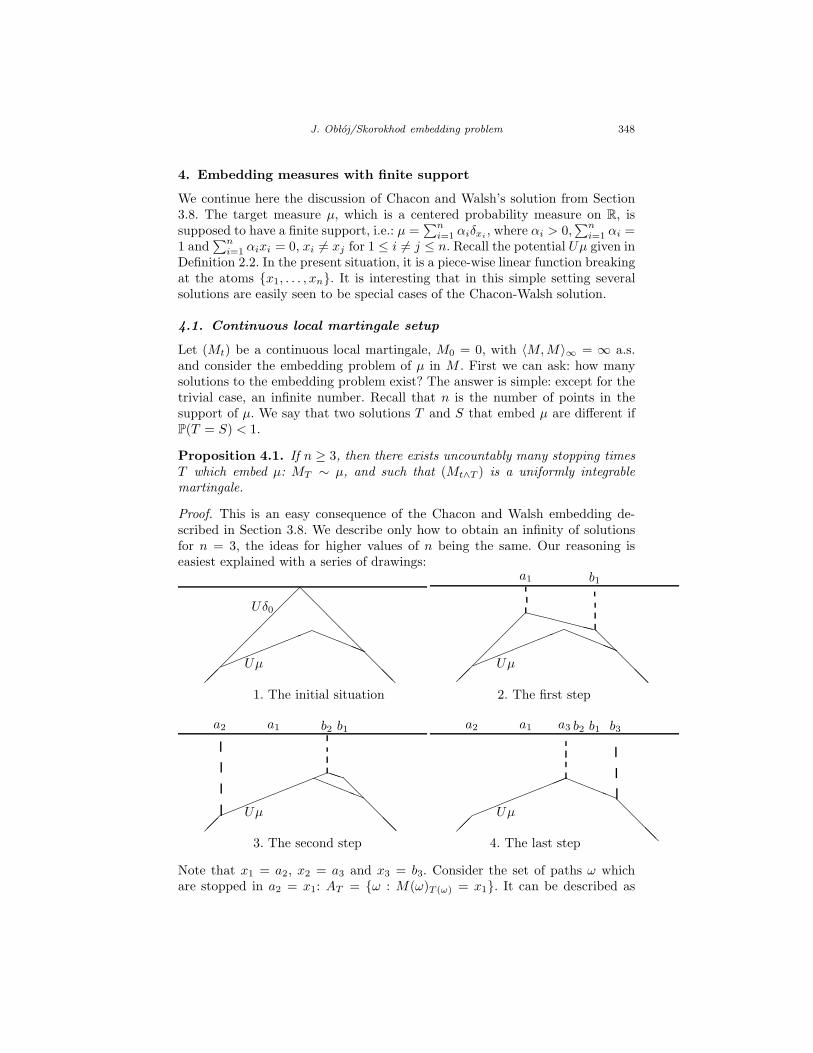
Proposition 4.1. If n ≥ 3, then there exists uncountably many stopping timesT which embed µ: MT ∼ µ, and such that (Mt∧T ) is a uniformly integrablemartingale.

Proof. This is an easy consequence of the Chacon and Walsh embedding de-scribed in Section 3.8. We describe only how to obtain an infinity of solutionsfor n = 3, the ideas for higher values of n being the same. Our reasoning iseasiest explained with a series of drawings:

Uδ0

Uµ

aaaaa!!!!!!!

@@

@@

@@

@@

@@

@@@

b1a1

XXXXXX

Uµ

aaaaa!!!!!!!

1. The initial situation 2. The first step

b2a2

!!!!!!!!

PP@

@@

@@

b1a1

Uµ

aaaa

b2a2

!!!!!!!!

@@

@@

b1a1

Uµ

aaaa

b3a3

3. The second step 4. The last step

Note that x1 = a2, x2 = a3 and x3 = b3. Consider the set of paths ω whichare stopped in a2 = x1: AT = ω : M(ω)T (ω) = x1. It can be described as


the set of paths that hit a1 before b1 and then a2 before b2. It is clear from ourconstruction that we can choose these points in an infinite number of ways andeach of them yields a different embedding (paths stopped at x1 differ). Indeedas for any a1 ≤ a1 < 0 < b2 < b2 < b1, P(Ta1

< Tb2< Ta1 < Tb1) > 0, the result

follows from the fact that if P(BT 6= BS) > 0 then P(S = T ) < 1.

However in their original work Chacon and Walsh allowed only to take linestangent to the graph of Uµ. In this case we have to choose the order of drawingn− 1 tangent lines and this can be done in (n− 1)! ways. Several of them areknown as particular solutions. Note that we could just as well take a measurewith a countable support and the constructions described below remain true.

• The Azema-Yor solution consists in drawing the lines from left to right.This was first noticed, for measures with finite support, by Meilijson [73].The Azema-Yor solution can be summarized in the following way. Let X ∼µ. Consider a martingale Yi = E[X |1X=x1 , . . . ,1X=xi

], Y0 = 0. Note thatYi has dichotomous transitions, it increases and then becomes constantand equal to X as soon as it decreases, Yn−1 = X . Embed this martingaleinto (Mt) by consecutive first hitting times. It suffices to remark nowthat the hitting times correspond to ones obtained by taking tangent linesin Chacon and Walsh construction, from left to right. Indeed, the lowerbounds for the consecutive hitting times are just atoms of µ in increasingorder from x1 to xn−1.

Another way to see all this is to use the property that the Azema-Yorsolution maximizes stochastically the maximum of the process. If we wantthe supremum of the process to be maximal we have to take care notto “penalize big values” or in other words “not to stop too early in asmall atom” - this is just to say that we want to take the bounds of ourconsecutive stopping times as small as possible, which is just to say wetake the tangent lines from left to right.

Section 5 is devoted to the study of this particular solution in a generalsetting.

• The Reversed Azema-Yor solution consists in taking tangents fromright to left. It minimizes the infimum of the stopped process. We discussit in Section 5.3.

• The Dubins solution is always a particular case of the Chacon and Walshsolution. In a sense it gives a canonical method of choosing the tangents.We described it in Section 3.8.

4.2. Random walk setup

When presenting above, in Section 3.8, the Chacon and Walsh solution, wepointed out that it only takes advantage of the martingale property of Brown-ian motion. We could ask therefore if it can also be used to construct embeddingsfor processes with countable state space. And it is very easy to see the answer


is affirmative, under some hypothesis which guarantees that no over-shoot phe-nomenon can take place.

Let (Mn)n≥0 be a discrete martingale taking values in Z with M0 = 0 a.s.Naturally, a symmetric random walk provides us with a canonical example andactually this section was motivated by a question raised by Fujita [44] concerningprecisely the extension of the Azema-Yor embedding to random walks.

Denote the range of M by R = z ∈ Z : infn ≥ 0 : Mn = z <∞ a.s. andlet µ be a centered probability measure on R. It is then an atomic measure6. Wecan still use the Chacon and Walsh methodology under one condition. Namely,we can only use such exit times Ta,b that both a, b ∈ R. Otherwise we wouldface an over-shoot phenomena and the method would not work.

Naturally in the Azema-Yor method, the left end points, (ak), are just theconsecutive atoms of µ, which by definition are in R. The right-end points aredetermined by tangents to Uµ as is described in detail in Section 5.1 below.They are given by Ψµ(ak), where Ψµ is displayed in (5.2), and they might notbe in R.

Proposition 4.2. In the above setting suppose that the measure µ is such thatΨµ(R) ⊂ R, where Ψµ is given by (5.2). Then the Azema-Yor stopping time,T = infn ≥ 0 : Sn ≥ Ψµ(Mn), where Sn = maxk≤n Mk, embeds the measureµ in M , MT ∼ µ.

The same Proposition, for a random walk, was also obtained by Fujita [44].He used discrete martingales, which are closely related to the martingales usedby Azema and Yor [3] in their original proof, and which we discuss in Section5.4.

We close this section with two observations. First, notice that the conditionΨµ(R) ⊂ R is not necessary for the existence of a solution to the Skorokhodembedding problem. We give a simple example. Consider a standard, symmetricrandom walk, (Xn : n = 0, 1, . . . ), and take µ = 2

9δ−3 + 49δ0 + 1

3δ2. ThenΨµ(0) = 6

7 /∈ Z, but one can easily point out a good embedding. It suffices totake tangents to Uµ from right to left, that is to consider the reversed Azema-Yor solution. Then the stopping time T = infn ≥ T−1,2 : Mn /∈ [−3, 0] embedsµ in M .

Finally, it is not true that for any centered discrete probability measure µ,there exists a stopping time T , in the natural filtration of X , such that XT ∼ µand (Xn∧T : n ≥ 0) is a uniformly integrable martingale. This was observed byCox [21]. It suffices to take µ = 1

3 (δ−1 +δ0 +δ1) (one can also impose µ(0) = 0and still find easy examples). Therefore, for some measures, a solution to theSkorokhod embedding problem for random walk has to rely on an externalrandomization. This subject requires further investigation.

5. Around the Azema-Yor solution

In this section we present various results concerning the solution proposed byAzema and Yor [3]. We first provide a very simple proof of the solution in

6The support is not necessary finite but this is not crucial for the method, so we decidedto place this discussion in this section.


Section 5.1. The proof is based on the methodology of Chacon and Walsh (seeSection 3.8) and allows us very easily to generalize the Azema-Yor embeddingfor the case of nontrivial initial laws. This is done in Section 5.2. The proofencouraged us too to give, in Section 5.3, another, reversed, form of the solution.In subsequent Section 5.4, we explain the original ideas, based on martingaletheory, which stood behind the work of Azema and Yor. This allows us, inSection 5.5 to prove easily certain extremal properties of this solution.

We give first a brief history of this solution. It was presented in the 13th

“Seminaire de Probabilites” in [3] together with a follow up [2], which examinedsome maximizing property (see Section 5.5 below) of the solution. The originalarguments are also found in Revuz and Yor ([99] pp. 269–276). The constructionin [3] was carried out for a continuous local martingale and extended easily torecurrent, real-valued diffusions. The original proof was then simplified by Pierre[95] and Vallois [118]. A proof using excursion theory was given by Rogers [101].An elementary proof was given by Zaremba [126]. This work [126] not only givesa “bare-handed” proof, but doing so it actually provides a convenient limitingprocedure that allows us to see that Azema and Yor’s solution is, in a sense, aspecial case of Chacon and Walsh’s solution (see also Section 4). The Azema-Yor solution has been generalized by several authors - we described their paperstogether in Section 3.17. Finally, using Levy’s equivalence (S−B,S) ∼ (|B|, L),works using the local time at 0 to develop a solution to the embedding problemcan be seen as generalizing Azema and Yor’s construction, and we mentiontherefore articles by Jeulin and Yor [60] and by Vallois [118] (see Section 3.12).

5.1. An even simpler proof of the Azema-Yor formula

In this section, for simplicity of notation, we write “AY solution” for Azemaand Yor’s solution.

We saw in Section 4 how the AY construction for a measure with finitesupport is just a special case of the method described by Chacon and Walsh,and consists in taking as tangent lines the extensions of the linear pieces of thepotential from left to right. In this section we will see how to generalize thisidea.

Let µ be a centered probability measure on R and x a point in the interiorof its support, such that µ has no atom at x: µ(x) = 0. Recall the one-dimensional potential given in Definition 2.2. We are interested in the tangentline lx to Uµ at (x, Uµ(x)) and its intersection with the line (t,−t) : t ∈ R.Denote this intersection by (Ψµ(x),−Ψµ(x)). The following drawing summa-rizes these quantities:


x

lx

Ψµ(x)

@@

@@

@@

@@

.

It is straightforward to find the equation satisfied by lx. Its slope is given bydUµ(t)

dt |t=x and so we can write lx = (x, y) : y = dUµ(t)dt |t=x · x+ β. Differenti-

ating (2.3) we obtain

dUµ(t)

dt= 2µ([t,∞)) − 1 − 2tµ(dt) + 2tµ(dt)

= 2µ([t,∞)) − 1. (5.1)

We go on to calculate β. Using the fact that (x, Uµ(x)) ∈ lx together with (2.3)and (5.1), we obtain β = −2

∫

[x,∞)ydµ(y). We are ready to determine the value

of Ψµ(x) writing the equation of the intersection of lx with (t,−t) : t ∈ R:

−Ψµ(x) =(

2µ([x,∞)) − 1))

Ψµ(x) − 2

∫

[x,∞)

ydµ(y), hence

Ψµ(x) =1

µ([x,∞))

∫

[x,∞)

ydµ(y), (5.2)

which is just the barycentre function defined by Azema and Yor, which is alsocalled the Hardy-Littlewood (maximal) function. We still have to deal howeverwith atoms of µ. Clearly in atoms the potential is not differentiable and thetangent is not unique. It is easy to see from the construction of Ψµ(x) that itis a non-decreasing, continuous function (for x with µ(x) = 0). Fix an x suchthat µ(x) > 0. To assign value to Ψµ(x) we follow the case of measures withfinite support described in Section 4. We see that, as a consequence of takingthe tangents from left to right, we treat the point (x, Uµ(x)) as belonging ratherto the linear piece of the potential on the left than the one on the right. In otherwords we take Ψµ to be left continuous. The formula (5.2) remains valid for allx in the interior of support of µ then.

We want finally to describe the function Ψµ outside of the support of µ(and on its boundaries). Suppose that the support of µ is bounded from below:aµ = infx : x ∈ supp(µ) > −∞. For all x ≤ aµ we have simply that Uµ(x) = xand so the tangent is just the line (t, t) : t ∈ R, which intersects the line(t,−t) : t ∈ R in (0, 0), so we put Ψµ(x) = 0.

Suppose now that the support of µ is bounded from above: bµ = supx :x ∈ supp(µ) < ∞. Then for all x ≥ bµ we have Uµ(x) = −x and so the verypoint (x, Uµ(x)) lies on the line (t,−t) : t ∈ R and we put Ψµ(x) = x. Thiscompletes the definition of the function Ψµ, which coincides with the one givenin [3].


We want now to define the stopping time that results from this setup. Atfirst glance we could have a small problem: following closely the case of measureswith finite support would end up in a composition of an uncountable infinity offirst hitting times of intervals (x,Ψµ(x)) for x in the support of µ. This wouldnot make much sense. However there is an easy way to overcome this difficulty- we can use the fact that Ψµ is increasing. Let (Mt : t ≥ 0) be a continuouslocal martingale and denote its supremum by St = supMs : s ≤ t. St thendescribes which values of type Ψµ(x) have been reached so far, and so which ofthe intervals (x,Ψµ(x)) we are considering. We want to stop when exiting suchan interval on its left boundary, i.e. when we reach an x such that the supremumso far is equal to Ψµ(x). In other words we take:

TAY = inft ≥ 0 : St ≥ Ψµ(Mt). (5.3)

Theorem 5.1 (Azema and Yor [3]). Let (Mt)t≥0 be a continuous martingale,M0 = 0 a.s., with 〈M,M〉∞ = ∞ a.s. For any centered probability measure µon R, TAY defined through (5.3), is a stopping time in the natural filtrationof (Mt) and MTAY

∼ µ. Furthermore, (Mt∧TAY)t≥0 is a uniformly integrable

martingale.

Proof. From (5.3) it is evident that TAY is a stopping time in the naturalfiltration of (Mt). The proof of the remaining statements is carried out througha limit procedure using approximation of Uµ by piece-wise linear functions. Wedefine measures µn through their potentials. Let A = a1, a2 . . . be the set ofatoms of µ (i.e. µ(x) > 0 iff ∃! i : x = ai) and Pn = k

n : k ∈ Z. Define µn

through:

• ∀ x ∈ A ∪ Pn ∩ [−n, n] Uµn(x) = Uµ(x),

• Uµn is piece-wise linear, µn((−∞,−n− 1] ∪ [n+ 1,∞)) = 0.

It is straightforward that Uµn(x) → Uµ(x) for all x ∈ R, which in turn impliesµn ⇒ µ. For each of the measures µn consider the AY stopping time Tn, whichembeds µn as shown in Section 4. Finally from the definition of a tangent, wesee that lines defining Tn converge to tangents of Uµ and Tn → T = TAY almostsurely. Then MTn

→ MT a.s. and since µn ⇒ µ, we obtain MTAY∼ µ. To see

that (Mt∧TAY: t ≥ 0) one can use assertion (v) of Proposition 2.3 and the fact

that ETn =∫

x2dµn(x) <∞.

It has to be noted that what we did in this section is essentially a simplifiedreading of Zaremba’s work [126] - simplified through the work of Chacon andWalsh.

5.2. Nontrivial initial laws

One of the advantages of the approach presented here is that we impose onlyone condition on the initial law: namely that its potential is greater than thepotential of the measure µ we want to embed (and this is known to be a necessary


condition, see Section 8). We can still give an explicit formulae for the stoppingtime TAY, for nontrivial initial laws.

Let (Mt : t ≥ 0) be a continuous, local, real-valued martingale with 〈M,M〉∞ =∞ a.s. and with initial law M0 ∼ ν,

∫

|x|dν(x) < ∞. Let µ be any probabilitymeasure on R with finite first moment, i.e. µ ∈ M1, such that Uµ ≤ Uν. Usingassertion (ii) from Proposition 2.3, this implies

∫

xdν(x) =∫

xdµ(x) = m, and

lim|x|→∞

(Uν(x) + |x−m|) = lim|x|→∞

(Uµ(x) + |x−m|) = 0. (5.4)

Then µ can be embedded in M by a stopping time, which is a generalization ofAzema and Yor’s solution.

Consider a tangent to the potential Uµ at a point (x, Uµ(x)) (which is notan atom of µ). We want to describe the points of intersection of this line withthe potential of ν. Studying (2.3), (5.1) and (5.2) it is easily seen that the pointsare of form (t, Uν(t)), where t satisfies

Uν(t) =(

µ([x,∞)) − µ((−∞, x)))

t+

∫ x

−∞ydµ(y) −

∫ ∞

x

ydµ(y). (5.5)

We want to define a generalized barycentre function Ψνµ(x) as a certain solution

of the above and the stopping time will be given as usual through

T ν,µAY

= inft ≥ 0 : St ≥ Ψνµ(Bt). (5.6)

Let us look first at a simple example. Let B be a Brownian motion starting fromzero and ν ∈ M1

0 be concentrated on a and b, in other words ν ∼ BTa,b. Then

µ is also centered as Uµ ≤ Uν. Let aµ = inft : t ∈ supp(µ) ≤ a be the lowerbound of the support of µ and Ψµ be the standard barycentre function definedthrough (5.2). Writing the explicit formula for Uν in (5.5) we obtain

Ψνµ(x) =

a , for x ≤ aµ∫

[x,∞)ydµ(y)+ ba

b−a

µ([x,∞))+ ab−a

, for aµ < x < b

Ψµ(x) , for x ≥ b.

Consider now the general setup. The equation (5.5) has either two solutionst1x < t2x or solutions form an interval t ∈ [t−x , t

+x ], t−x ≤ t+x , see Figure 1. Let us

denote these two situations respectively by I and II. The latter happens if andonly if the two potentials coincide in x. Finally, for a probability measure ρ letaρ = inft : t ∈ supp(ρ), bρ = supx : x ∈ supp(ρ) be respectively the lowerand the upper bound of the support of ρ. Define:

Ψνµ(x) =

aν , for x ≤ aµ

t2x , for aµ < x < bµ if Ix for (aµ < x < bµ if II) and for (x ≥ bµ).

(5.7)

A simple observation is required to see that the definition agrees with the intu-ition. Since Uµ ≤ Uν ≤ Uδm, and Uµ and Uν coincide with Uδm outside their


Uµ Uν

t+xt−x

@@

@@

@

t2yt1yyx

aaaaaa

Figure 1: Possible intersections of tangents for nontrivial initial law.

supports, the support of ν is contained in the support of µ, [aν , bν ] ⊂ [aµ, bµ].This grants that Ψν

µ(x) ≥ x.It is also worth mentioning that the function Ψν

µ lost some of the propertiescharacterizing Ψµ. In particular we can have Ψν

µ(x1) = x1 and Ψνµ(x2) > x2, for

some x2 > x1.

Proposition 5.2. Let (Mt : t ≥ 0) be a continuous, real-valued, local martingalewith 〈M,M〉∞ = ∞, M0 ∼ ν, and µ ∈ M1 with Uµ ≤ Uν. Define Ψν

µ and T ν,µAY

through (5.7) and (5.6) respectively. Then (Mt∧T ν,µ

AY

) is a uniformly integrablemartingale and MT ν,µ

AY

∼ µ.

The proof of this result is analogous to the proof of Theorem 5.1, taking intoaccount the above discussion of Ψν

µ.We remark that the construction presented above might be used to mix or

refine some of the known solutions to the embedding problem. For example ifµ([−a, a]) = 0 we can first stop at T−a,a and then use T ν,µ

AYwith ν = 1

2 (δ−a +δa).

5.3. Minimizing the minimum - the reversed AY solution

In Section 5.1 we saw how to derive Azema and Yor’s solution to the Skorokhodproblem using potential theory. It is easy to see that the same arguments allowus to recover another solution, which we call the reversed Azema-Yor solution.It was first studied by van der Vecht [121] (see also Meilijson [74]). Recall thatlx was the tangent to the potential Uµ in (x, Uµ(x)). We considered its inter-section with the line (t,−t) : t ∈ R, which was denoted (Ψµ(x),−Ψµ(x)).Consider now the intersection of lx with the line (t, t) : t ∈ R and denote itby (Θµ(x),Θµ(x)). A simple calculation (analogous to the derivation of (5.2)above) shows that:

Θµ(x) =1

µ((−∞, x))

∫

(−∞,x)

ydµ(y). (5.8)

This is a valid formula for x which is not an atom. Looking at the discrete casewe see that we want Θµ to be right continuous, so we finally need to define:

Θµ(x) =1

µ((−∞, x])

∫

(−∞,x]

ydµ(y). (5.9)


Denote st = − infMs : s ≤ t the infimum process and define the followingstopping time

TrAY = inft ≥ 0 : −st ≤ Θµ(Mt). (5.10)

Corollary 5.3. Let (Mt)t≥0 be a continuous local martingale, M0 = 0 a.s., with〈M,M〉∞ = ∞ a.s. and let µ be a centered probability measure on R. Define Θµ

through (5.9). Then TrAY is a stopping time and Mt∧TrAY∼ µ. Furthermore,

(Mt∧TrAY: t ≥ 0) is a uniformly integrable martingale. As a consequence, if

∫

Rx2dµ(x) = v <∞ then ETrAY = v.

We called this a corollary as this solution is still an Azema-Yor solution.Indeed if X ∼ µ then TrAY is just TAY for ν the law of −X and the continuouslocal martingale Nt = −Mt. This shows also that we could handle non-trivialinitial laws for the reversed Azema-Yor solution. Speaking informally, in theoriginal Azema-Yor solution one takes tangents from left to right and in thereversed version one takes the tangents from right to left. We will see belowthat it yields some symmetric optimal properties.

5.4. Martingale theory arguments

In the preceeding, we chose to discuss the Azema-Yor solution using one-dimensionalpotential theory. This methodology allowed us to understand well what is re-ally being done and what is really being assumed, opening itself easily to somegeneralizations, as we saw above and as we will see again in Section 9. Onecan choose however a different methodology, which has its own advantages aswell. We sketch now the heart of the proof that goes through martingale theory.These are the ideas that actually led to the original derivation of the solutionin [3].

Let f : [0,∞) → R be an integrable function and denote its primitive byF (x) =

∫ x

0 f(y)dy. Then

Nft = F (St) − (St −Mt)f(St), t ≥ 0 (5.11)

is a local martingale, where M and S are as in the previous section. This canbe easily seen when f is continuously differentiable, since integrating by partswe obtain

NFt = F (St) −

∫ t

0

f(Su)dSu +

∫ t

0

f(Su)dMu −∫ t

0

(Su −Mu)f ′(Su)dSu

= F (St) − F (St) +

∫ t

0

f(Su)dMu =

∫ t

0

f(Su)dMu, (5.12)

as (Su −Mu) is zero on the support of dSu. The result extends to more generalfunctions f through a limit procedure7. Given a centered probability measureµ, we want to find T , which embeds µ, of the form T = inft ≥ 0 : St ≥

7It can also be verified for f an indicator function and then extended through the monotoneclass theorem. For more on martingales of the form (5.11) see [85]


Ψ(Mt). Our goal is therefore to specify the function Ψ. Suppose we can applythe optional stopping theorem to the martingale NF and the stopping time T .We obtain

EF (ST ) = E(ST −MT )f(ST ). (5.13)

Note that MT ∼ µ and ST = Ψ(MT ). We suppose also that Ψ is strictlyincreasing. If we denote by ρ the law of ST and ρ = ρ([x,+∞)) its tail, theabove equation can be rewritten as

∫

F (x)dρ(x) =

∫

(x − Ψ−1(x))f(x)dρ(x), integrating by parts

∫

f(x)ρ(x)dx =

∫

(x − Ψ−1(x))f(x)dρ(x), which we rewrite as

dρ(x) = − ρ(x)

x− Ψ−1(x)dx, since f was a generic function .

We know that ST = Ψ(MT ), so that µ(x) = P(MT ≥ x) = P(ST ≥ Ψ(x)) =ρ(Ψ(x)). Inserting this in the above yields

dµ(x) = d(

ρ(Ψ(x)))

= − ρ(Ψ(x))

Ψ(x) − xdΨ(x) = − µ(x)

Ψ(x) − xdΨ(x)

Ψ(x)dµ(x) − xdµ(x) = −µ(x)dΨ(x)

Ψ(x)dµ(x) + µ(x)dΨ(x) = xdµ(x)

d(

Ψ(x)µ(x))

= xdµ(x)

Ψ(x)µ(x) =

∫

[x,+∞)

ydµ(y),

and we find the formula (5.2).

5.5. Some properties

The Azema-Yor solution is known to maximize the supremum in the followingsense. Let µ, M and S be as in the previous section, and R any stopping timewith MR ∼ µ and (MR∧t : t ≥ 0) a uniformly integrable martingale. Then forany z > 0, P(SR ≥ z) ≤ P(STAY

≥ z). This was observed already by Azemaand Yor [2], as a direct consequence of work by Dubins and Gilat [32], which inturn relied on Blackwell and Dubins [8]. We will try to present here a unifiedand simplified version of the argumentation. The property was later argued inan elegant way by Perkins [90] and it is also clear from our proof in Section 5.1(as stressed when discussing measures with finite support, see page 349).

For simplicity assume that µ has a positive density, so that µ−1 is a welldefined continuous function. Let f(x) = 1[z,+∞)(x), then NF

t = (St − z)+ −(St −Mt)1[z,+∞)(St) is a martingale by (5.11). Applying the optional stoppingtheorem for (R ∧ n) and passing to the limit (using the monotone convergencetheorem and the uniform integrability of (MR∧t : t ≥ 0)) we see that z P(SR ≥


z) = EMR1[z,+∞)(SR). Denote P(SR ≥ z) = p. It suffices now to note, that

zp = EMR1[z,+∞)(SR) ≤ EMR1[µ−1(p),+∞)(MR)

=

∫ ∞

µ−1(p)

xdµ(x) = pΨµ

(

µ−1(p))

, thus

z ≤ Ψµ

(

µ−1(p))

, which yields

p ≤ µ(

Ψ−1µ (z)

)

= P(

MTAY≥ Ψ−1

µ (z))

= P(STAY≥ z),

which we wanted to prove. Note that the passage between the last two lines isjustified by the fact that Ψ−1

µ is increasing and µ is decreasing.This optimality property characterizes the Azema-Yor solution. Further-

more, it characterizes some of its generalizations - for example in the case ofBrownian motion with drift, see Peskir [93]. It also implies an optimality prop-erty of the reversed solution presented in Section 5.3. Namely, with R as above,we have P(sR ≥ z) ≤ P(sTrAY

≥ z), for any z ≥ 0, where st = − infu≤t Mu.The second optimality property says that this solution is pointwise the small-

est one. More precisely, if for any stopping time S ≤ TAY and MS ∼MTAYthen

S = TAY a.s. Actually, it is a general phenomena that we will discuss in Section8, along with some other general properties of stopping times.

6. The H1-embedding

Given a solution T to the Skorokhod stopping problem we can ask about thebehavior of supremum or infimum of our process up to time T . This questionhas attracted a lot of attention. In particular some solutions were constructedprecisely in order to minimize the supremum and maximize the infimum andconversely.

Let us denote by (Xt) the real valued process we are considering and µ aprobability measure on the real line. The following problem:

Find some necessary and sufficient conditions on (X,µ) for the existence ofa solution T to the Skorokhod embedding problem such that X∗

T = sup|Xs| :s ≤ T is in Lp,

is called the Hp-embedding problem. We will restrain ourselves to the Brow-nian setup, even though most of the ideas below work for real-valued diffusionson natural scale. We will present a solution of the Hp-embedding by Perkins. Heactually gives a solution to the Skorokhod embedding problem, which minimizesX∗

T . We then proceed to Jacka’s solution, which is a counterpart of Perkins, as itmaximizes X∗

T . We mention that several authors have investigated in detail thebehavior of the maximum of a uniformly integrable martingale and we gatheredtheirs works in Section 10.3.

6.1. A minimal H1-embedding

The problem of Hp-embedding was also considered by Walsh and Davis [27]but received a complete and accurate description in Perkins’ work in 1985 [90].Using Doob’s Lp-inequalities one can see easily that for p > 1 an Hp-embedding


exists if and only if∫

|x|pdµ(x) < ∞, and if p < 1 every embedding is in factan Hp-embedding. For p = 1 the situation is more delicate, and it goes back toan analytical problem solved by Cereteli [15].

Theorem 6.1 (Cereteli-Davis-Perkins). Consider Brownian motion and acentered probability measure µ. The following are equivalent:

• There exists an H1-embedding of µ.

• The Skorokhod solution, described in Section 3.1, is an H1-embedding ofµ.

• H(µ) =∫∞0

1λ |∫

Rx1|x|≥λdµ(x)|dλ <∞.

Perkins [90] associated with every centered probability measure two func-tions: γ− and γ+ (see the original work for explicit formulae). Then if

St = supu≤t

Bu and st = − infu≤t

Bu (6.1)

are respectively the supremum and infimum processes we can define:

ρ = inft > 0 : Bt /∈ (−γ+(St), γ−(st)). (6.2)

If the target distribution has an atom in 0, we just have to stop in 0 with theappropriate probability. This is done through an external randomization. Wetake an independent random variable U , uniformly distributed on [0, 1] and put

TP = ρ1U>µ(0), (6.3)

where P stands for Perkins. TP is a (randomized) stopping time that embeds µand TP is an H1-embedding if there exists one. Moreover, Perkins defined hisstopping time in order to control the law of the supremum and the infimum ofthe process and his stopping time is optimal.

Theorem 6.2 (Perkins). (Bt∧TP: t ≥ 0) is a uniformly integrable martingale

and BTP∼ µ. TP is an H1-embedding if and only if H(µ) < ∞. Furthermore,

for any solution T of the Skorokhod embedding problem for µ, for all λ > 0,

P(STP≥ λ) ≤ P(ST ≥ λ), (6.4)

P(sTP≥ λ) ≤ P(sT ≥ λ), (6.5)

P(B∗TP

≥ λ) ≤ P(B∗T ≥ λ). (6.6)

Actually this theorem is not hard to prove - the stopping time is constructedin such a way as to satisfy the above. The hard part was to prove that TP embedsµ. The construction of TP helps Perkins to give explicit formulae for the threeprobabilities on the left side of (6.4)-(6.6). Using Perkins’ framework we couldalso define a different stopping time in such a way that it would maximizestochastically the supremum S. Of course what we end up with is the Azema-Yor stopping time (see Sections 5.1 and 5.5) and this is yet an another approachwhich allows us to recover their solution in a natural way.


The work of Perkins has been generalized by Cox and Hobson [23, 24]. Severalauthors examined the law of supremum (and infimum) of a martingale with afixed terminal distribution (see Section 10.3). More generally, the link betweenthe Skorokhod embedding problem and optimal stopping theory was studied.We develop this subject in Section 10.

6.2. A maximal H1-embedding

We saw in Section 5 that the Azema-Yor construction maximizes stochasticallythe distribution of ST , where BT ∼ µ, fixed, in the class of stopping times suchthat (Bt∧T )t≥0 is a uniformly integrable martingale. Moreover, we saw also thatits reversed version TrAY, minimizes the infimum. How can we combine thesetwo? The idea came from Jacka [58] and allowed him to construct a maximal H1

embedding. We will describe his idea using the Chacon and Walsh methodology,which is quite different from his, yet helps, in our opinion, to see what is reallybeing done.

We will continue to work within the Brownian setting, even though ev-erything works in exactly the same way for continuous local martingales. Wewant to find a stopping time T such that BT ∼ µ, (Bt∧T : t ≥ 0) is a uni-formly integrable martingale and if R is another such stopping time, thenP(B∗

R ≥ z) ≤ P(B∗T ≥ z), for z ≥ 0. Naturally big values of B∗ come ei-

ther from big values of S or s. We should therefore wait “as long as possible”to decide which of the two we choose, and then apply the appropriate extremalembedding. To see whether we should use big negative or big positive valueswe will stop the martingale at the exit time from some interval [−k, k], whichwe assume to be symmetric. This corresponds to cutting the initial potentialwith a horizontal line. The biggest value of k which we can take is obtained byrequiring that the horizontal line be tangent to the potential Uµ.

For sake of simplicity we suppose that the measure µ has a positive density.We need to determine the point x∗ in which the derivative of Uµ becomes zero.Looking at (5.1) we see that µ(x∗) = 1

2 . In other words, we chose the median ofµ for x∗. The value of k∗ is then given as the intersection of the tangent to thegraph of Uµ in x∗ with the line y = −x, which is precisely k∗ = Ψµ(x∗), whereΨµ is given by (5.2).

As suggested, we first stop at the exit time from [−k∗, k∗]. Obviously Brow-nian motion stops either at k∗, in which case it will be finally stopped in-side [Uµ(x∗),∞), or at −k∗ in which case it will be finally stopped inside(−∞, Uµ(x∗)]. If we exit at the top, we want to maximize the supremum, andso we will use the standard Azema-Yor embedding: T1 = inft > T−k,k : St ≥Ψµ(Bt). If we exit at the bottom, we need to minimize the infimum, so we willuse the reversed Azema-Yor solution: T2 = inft > T−k,k : −st ≤ Θµ(Bt). Wehave then the following proposition,

Proposition 6.3 (Jacka [58]). In the above setup

P(

B∗R ≥ z) ≤ min

1, µ([ψ−1µ (z),+∞)) + µ((−∞,Θ−1

µ (z)])

. (6.7)


Furthermore, this inequality is optimal as equality is attained for a stopping timeTJ defined through

TJ = T1 ∧ T2 = inf

t ≥ T−k∗,k∗ : B∗t ≥ max(Ψµ(Bt),Θµ(Bt)

. (6.8)

If the measure µ has atoms the above Proposition is still true taking left in-verses of Ψµ and Θµ and extending correctly the definition of k∗. More precisely,if we write m = infx : µ(x) ≥ 1

2 for the median of µ, then if µ(m) > 0 wehave a family of tangents to Uµ in m. The value Ψµ(m) results from taking theleft-most tangent (cf. Section 5.1) and not the horizontal one. We have there-fore k∗ > Ψµ(m). The difference is given by the slope of the left-most tangent,(2µ(m) − 1), times the increment interval (Ψµ(m) −m). We obtain therefore:k∗ = Ψµ(m) + (2µ(m)− 1)(Ψµ(m)−m), which is the quantity given in Lemma6 in Jacka [58].

7. Root’s solution

All the solutions described so far have one thing in common: stopping times aredefined through some functionals of Brownian motion up to time T . Intuitively,if one searches for a stopping time with minimal variance it should have avery simple history-dependence structure, preferably it should just be the firsthitting time of some set. Of course this cannot be just a subset of the spaceR but rather of the time-space R+ ×R. Root [103] showed that indeed for anycentered probability measure µ on R with finite second moment, there exists aset Rµ ⊂ R+ ×R, such that the first entrance time of (t, Bt) into Rµ, embedsµ in Brownian motion B. The first hitting times for the space-time process ofBrownian motion correspond to reduites of potential measures and we should notbe surprised that to investigate Root’s solution Rost [104], [105], [106] needed afair amount of potential theory.

7.1. Solution

The key notion is that of a barrier.

Definition 7.1. A subset R of [0,+∞] × [−∞,+∞] is a barrier if

1. R is closed,

2. (+∞, x) ∈ R for all x ∈ [−∞,+∞],

3. (t,±∞) ∈ R for all t ∈ [0,+∞],

4. if (t, x) ∈ R then (s, x) ∈ R whenever s > t.

Theorem 7.2 (Root [103]). For any probability measure µ on R with∫

x2dµ(x) =v < ∞ and

∫

xdµ(x) = 0, there exists a barrier Rµ such that the first hittingtime of the barrier

T µR

= TRµ= inft ≥ 0 : (t, Bt) ∈ Rµ, (7.1)

solves the Skorokhod problem for µ, i.e. BTRµ∼ µ and ETRµ

= v.


Remark on notation: We write T µR

for Root’s stopping time, which solves theSkorokhod embedding problem for the measure µ and TR for a general “Root’sstopping time” that is for the first hitting time of some barrier R. We write TRµ

for the first hitting time of a particular barrier Rµ.

The proof is carried out through a limit procedure. It is not hard to see thata barrier Rµ exists for a measure with finite support µ =

∑ni=1 αiδxi

. Rµ is justof the form

Rµ =

(

n⋃

i=1

[bi,+∞]×xi)

∪(

[0,+∞]× [−∞, x1]∪ [0,+∞]× [xn,+∞])

. (7.2)

The points (bi) are not given explicitly but only their existence is proven. Onethen needs some technical observations in order to pass to the limit.

Let H denote the closed half plane, H = [0,+∞] × [−∞,∞]. Root [103]defines a metric r on the space C of all closed subsets of H . Map H homeomor-phically to a bounded rectangle F by (t, x) → ( t

1+t ,x

1+|x|). Let F be endowed

with the ordinary Euclidean metric ρ and denote by r the induced metric on H .For C,D ∈ C put

r(C,D) = maxsupx∈C

r(x,D), supy∈D

r(y, C). (7.3)

Equipped with r, C is a separable, compact metric space and R, the subspaceof all barriers is closed in C and hence compact. Furthermore, this metric allowsus to deal with convergence in probability of first hitting times of barriers. Moreprecisely, the application which associates with a barrier R its first hitting time,i.e. R → TR, is uniformly continuous from (R, r) into the set of first hittingtimes of barriers equipped with convergence in probability.

Lemma 7.3 (Root [103], Loynes [70]). Let R be a barrier with correspondingstopping time TR. If P(TR <∞) = 1, then for any ǫ > 0 there exists δ > 0 suchthat if R1 ∈ R and r(R,R1) < δ then P(|TR − TR1 | > ǫ) < ǫ, where TR1 isdefined via (7.1). If P(TR = ∞) = 1 then for any K > 0 there exists δ > 0 suchthat r(R,R1) < δ implies P(TR1 < K) < ǫ.

If a sequence of barriers converges, Rnr−−−−→

n→∞R with E TRn

< K <∞, then

ETR ≤ K and P(|TRn− TR| > ǫ)−−−−→

n→∞0.

With this lemma the theorem is proven taking a sequence µn of probabilitymeasures with finite supports converging to µ, µn ⇒ µ.

7.2. Some properties

We start with some easy properties and then pass to the more involved resultsof Rost. The first property, established by Root [103] for his stopping time,asserted the equivalence between integrability of B2k

TRand T k

R, for k ∈ N. We

quoted it, in a more general form, in Preliminaries (Proposition 2.1) as it istrue for any stopping time T such that (Bt∧T : t ≥ 0) is a uniformly integrablemartingale.


Several further properties were described by Loynes [70], one of which isparticularly important for us. In order to state it, we need to introduce thenotion of a regular barrier. Let R ∈ R be a barrier. Define

xR+ = inf

y ∈ [0,∞] : [0,+∞] × y ⊂ R

xR− = supy ∈ [−∞, 0] : [0,+∞] × y ⊂ R, (7.4)

the first coordinates above and below zero respectively at which R is a horizontalline.

Definition 7.4. We say that a barrier R ∈ R is regular if [0,+∞]×[xR+,+∞] ⊂

R and [0,+∞] × [−∞, xR−] ⊂ R.

We say that two barriers R1, R2 are equivalent, R1 ∼ R2, if xR1− = xR2

− ,

xR1+ = xR2

+ and the two barriers coincide on [0,+∞] × [xR1− , xR1

+ ].

Thus a regular barrier R is one that is composed of horizontal lines above xR+

and below xR−. Clearly each barrier is equivalent to exactly one regular barrier.

Furthermore, for a barrier R we have that TR ≤ TxR−

,xR+

and so stopping times

corresponding to two equivalent barriers R1 ∼ R2 are equal TR1 = TR2 . Thisshows that we can limit ourselves to regular barriers.

Proposition 7.5 (Loynes [70]). Let µ be a centered probability measure on Rwith

∫

x2dµ(x) = v <∞. Then there exists exactly one regular barrier Rµ, suchthat BTRµ

∼ µ and ETRµ= v.

Loynes showed also that a wider class of probability measures µ can be em-bedded in Brownian motion through Root’s construction. However, the unique-ness result does not carry over to this more general setup.

The fundamental property of Root’s construction is that it minimizes thevariance of the stopping time. This conjecture, made by Kiefer [64], was provedby Rost.

Theorem 7.6 (Rost [107]). Let µ be a centered probability measure on Rwith

∫

x2dµ(x) = v < ∞ and let T µR

denote Root’s stopping time embedding µ.Assume that E(T µ

R)2 < ∞. Then, for any stopping time S such that BS ∼ µ

and ES = v, we have: E(T µR

)2 ≤ ES2 and E(T µR

)2 = ES2 if and only if S = T µR

a.s.More generally, for any 0 < p < 1, E(T µ

R)p ≥ ESp and for any p > 1, E(T µ

R)p ≤

ESp.

We will try to explain briefly, and at an intuitive level, how to arrive atthe above result. Actually, Rost considers the more general setup of a Markovprocess (that is assumed transient for technical reasons but the extension isfairly simple).

As in Section 2.2, let (Xt : t ≥ 0) be a Markov process (relative to its naturalfiltration (Ft)) on a compact metric space E associated with a semigroup (PX

t )and a potential kernel UX . Let ν and µ be two probability measures on the Borel


sets of E with σ-finite potentials µUX and νUX . The measure ν is the initiallaw: X0 ∼ ν and µ is the law we want to embed. Recall the characterizationof the balayage order given in Section 3.5. For existence of an embedding, themeasures have to satisfy µUX ≤ νUX . Then, there exists a stopping time Twhich embeds µ, µ = νPX

T .We are looking for a stopping time T with minimal variance. It is shown

actually that it satisfies the stronger property of minimizing Eν

∫ T

t∧T f(Xs)dsfor Borel, positive functions f , and any t > 0. This in turn is equivalent tominimizing νPX

t∧TUX for all t > 0. The idea is to look at the space-time process.

We consider a measure N on E × R defined through

N(A× B) =

∫

BNt(A)dt, where Nt = νUX1t<0 + νPX

t∧TUX1t≥0.

We take its reduite N (with respect to the semigroup of the space-time process)and show that it is of the form

N(A× B) =

∫

BNt(A)dt,

with N. decreasing, right continuous and Nt = νPXTR∧tU

X for a certain stopping

time with νPXTR

= µ. It follows that TR minimizes νPXt∧TU

X . The last stepconsists in showing that TR is actually Root’s stopping time for a certain barrierR. This is not surprising after all, as we saw that reduites are realized as hittingtimes of some sets and Root’s stopping time is just a hitting time for the space-time process.

7.3. The reversed barrier solution of Rost

In this section we describe a solution proposed by Rost, which is a counterpartfor Root’s solution as it maximizes the variance of the stopping time. We havenot found it published anywhere and we cite it following the notes by Meilijson[74]. The basic idea is to look at reversed barriers. Intuitively we just substitutethe condition that if a point belongs to a barrier then all the points to the rightof it also belong to the barrier, by a condition that all the points to the left ofit also belong to the barrier.

Definition 7.7. A subset ρ of [0,+∞]× [−∞,+∞] is called a reversed barrierif

1. ρ is closed,

2. (0, x) ∈ ρ for all x ∈ [−∞,+∞],

3. (t,±∞) ∈ ρ for all t ∈ [0,+∞],

4. if (t, x) ∈ ρ then (s, x) ∈ ρ whenever s < t.


Theorem 7.8 (Rost). For any probability measure µ on R with µ(0) = 0,∫

x2dµ(x) = v < ∞ and∫

xdµ(x) = 0, there exists a reversed barrier ρµ suchthat the stopping time

Tρµ= inft > 0 : (t, Bt) ∈ ρµ, (7.5)

solves the Skorokhod problem for µ, i.e. Bρµ∼ µ and E Tρµ

= v. Furthermore,if S is a stopping time such that BS ∼ µ and ES = v then for any p < 1ET p

ρµ≤ ESp, and for any p > 1 ET p

ρµ≥ ESp.

Note that there is a certain monotonicity in the construction of a reversedbarrier, which is not found in the construction of a barrier. For a point x in thesupport of µ, say x > 0, we must have the following property: there exists sometx such that (tx, x) ∈ ρµ and (tx, y) /∈ ρµ for any y ∈ [0, x). In other words,the reversed barrier ρµ, on the level x, has to extend “more to the right” thananywhere below, between 0 and x. This, in a natural way, could lead us to revisethe notion of a reversed barrier and introduce regular reversed barriers, whichwould satisfy ∀x > 0 if (t, x) ∈ ρ then (t, y) ∈ ρ, ∀y ∈ [x,+∞) and likewisefor x < 0. We could then obtain uniqueness results for Rost’s embedding in ananalogy to Proposition 7.5 above. We do not pursue these matters here, but wenote that, according to our best knowledge, they have never been investigated.

7.4. Examples

Explicit Root’s or Rost’s solutions are very rarely known, still we can give someexamples. First, a trivial example deals with Gaussian measures. If µ = N (0, v)then the barrier Rv = (t, x) : t ≥ v yields a deterministic stopping timeTRv

= v, which naturally embeds the measure µ.More sophisticated examples deal with square root boundaries. Shepp [113]

and Breiman [10], independently, considered the following stopping times8:

σa,c = inft ≥ 0 : |Bt| = c√t+ a.

These are easily seen to be Rost’s stopping times as σa,c = Tρa,c, where ρa,c =

(t, x) ∈ R+ ×R : x2 ≥ c(t + a) is a reversed barrier. As Bσa,c= c

√σa,c + a,

to characterize the law of Bσa,c, it suffices to characterize the law of σa,c, which

in turn is equivalent to giving its Laplace transform. This can be done usingexponential martingales or through a reduction to the first hitting times of agiven level for a radial Ornstein-Uhlenbeck process. We do not give the explicitformulae and refer to Going-Jaeschke and Yor [45] (see for example the formulaeon page 322) for a recent and extensive study which includes the subject.

Novikov [82] considered the following stopping time:

τa,b,c = inft ≥ 0 : Bt ≤ −a+ b√t+ c, (7.6)

8More precisely, Breiman [10] worked with T = inft ≥ 1 : Bt ≥ c√

t conditionally onB1 = 0.


where a ≥ 0, c ≥ 0 and bc1/2 < a. This is Root’s stopping time for a barrierRa,b,c = (t, x) ∈ R+ ×R : x ≥ −a + b

√t+ c, TRa,b,c

= τa,b,c. Again, charac-terizing the law of Bτa,b,c

is equivalent to characterizing the law of τa,b,c itself.To do so Novikov used a general family of exponential martingales of Brownianmotion and the optional stopping theorem. In particular Novikov showed thatE τv

a,b,c < ∞ if and only if b > z2v, where zv is the largest root of the equationDv(z) = 0, for Dv the parabolic cylinder function of the parameter v.

The stopping times σa,c and τa,b,c served Davis [26] to attain the optimallower and upper bounds on the proportion E |BT |p/ET p/2, where T is a stop-ping time, ET p/2 < ∞, p > 1. This is not surprising, as we would expect thatto attain the bounds one would have to consider stopping times which, withdistribution of BT fixed, minimize and maximize the expectation ET p/2, thatis Root’s and Rost’s stopping times (cf. Theorems 7.6 and 7.8).

Finally we mention two more papers which involve explicit calculations forRoot’s and Rost’s stopping times. For a barrier R it is naturally possible thatP(TR = ∞) > 0. Robbins and Sigmund [100] calculate the probabilities P(TR =∞) or P(TR ≥ u), u fixed, for the barriers of the type R = (t, x) : x ≥ f(t),where f is a function from a special family, which includes functions such asf(t) = ct+ a or f(t) =

√

(t+ ǫ) log(t+ ǫ). Lebedev [69] has calculations, for anarbitrary d-dimensional diffusion, of the first moment of Rost’s stopping timeswhich are the first passage times through a time-dependent, smooth boundaries.

7.5. Some generalizations

The problem we want to solve is a certain generalization of the one solvedby Rost. In [107] Rost showed that among all stopping times which solve agiven Skorokhod embedding problem, the stopping time defined by Root hasminimal second moment (which is equivalent to having minimal variance). Inthe Skorokhod embedding problem, the distribution of BT is fixed. Here we onlyfix two moments of this distribution and want to find the stopping time withthe minimal variance. That is:

Problem. Let us fix 4 > p > 1 and a constant cp > 0. Among all stopping timesT such that EBT = 0, ET = EB2

T = 1 and E|BT |p = cp, find the element Tmin

with minimal variance.

This problem is also linked with the optimal bounds on E |BT |p/ET p/2 obtainedby Davis [26], which we mentioned in the previous section. Davis [26] gives asolution to our problem without the restriction E |BT |p = cp.

Unfortunately, we did not succeed in solving this problem. We know it hasa solution and we will present a certain conjecture about it.

Proposition 7.9. The stopping time Tmin exists.

Proof. Recall Definition 7.1 and (7.1). It is an immediate observation that thestopping time we are looking for will be Root’s stopping time TR for some barrierR. Indeed, if the µ ∼ BTmin

is the distribution of BTmin, then there exists a

barrier Rµ such that Root’s stopping time TRµyields BTRµ

∼ µ. Moreover,


from Theorem 7.6, we know that ET 2Rµ

≤ ET 2min and so ET 2

Rµ= ET 2

min fromthe definition of Tmin. Therefore, using Theorem 7.6 again, we conclude thatTRµ

= Tmin a.s.We can limit ourselves to Root’s stopping times. Let

Acp=

µ ∈M1(R) :

∫

xµ(dx) = 0,

∫

x2µ(dx) = 1,

∫

|x|pµ(dx) = cp

.

For every µ ∈ Acpthere exists a unique regular barrier Rµ such that BTRµ

∼ µ.Let Rcp

be the subset of regular barriers corresponding to the measures in Acp.

Let H denote the closed half plane and recall the definition (7.3) of themetric r, under which C the space of all closed subsets of H , is a separable,compact metric space and R, the subspace of all barriers, is closed in C andhence compact.

We can introduce an order relation in Rcpgiven by: C 4 D ⇔ ET 2

C ≤ ET 2D,

for C,D ∈ Rcp. If we prove that there exists Rmin - a minimal element of Rcp

relative to 4 - then, we will have Tmin = TRmin. In other words

If there exists a Rmin ∈ Rcpsuch that

ET 2Rmin

= infR∈Rcp

ET 2R, then Tmin = TRmin

.

To complete the proof we need to show that Rcpis closed under r. Indeed,

choose a sequence of barriers Rn ∈ Rcp, such that ET 2

Rnց infR∈Rcp

ET 2R. We

can suppose that Rn converges (possibly choosing a subsequence) in r to somebarrier R. To conclude that R = Rmin we need to know that R ∈ Rcp

, whichfollows if Rcp

is a closed subset of R.In order to prove that Rcp

is a closed subset of R we essentially follow the

ideas used by Root in the proof of Theorem 7.2. Take any sequence Rnr→ R

with Rn ∈ Rcp. Then ETRn

= 1 for all n. It follows from Lemma 7.3 that forany ǫ > 0, P(|TR − TRn

| > ǫ)−−−−→n→∞

0 and ETR < ∞. Choosing a subsequence,

we may assume that TRn→ TR a.s. Furthermore, we can always construct a

measure µ ∈ Acpwith

∫

x4dµ(x) <∞, which implies ET 2Rµ

<∞ by Proposition

2.1, so that we may assume the sequence TRnis bounded in L2, and therefore

uniformly integrable, hence converges in L1. In particular ETR = 1. Finally,Proposition 2.1 also grants the existence of a universal constant C4, such thatEB4

T ≤ C4ET 2, which implies that the sequence (BTRn) is bounded in L4.

It converges almost surely, thanks to the continuity of paths and therefore itconverges in Lp. We see then, that E|BTR

|p = cp. This implies that R ∈ Rcp

and proves that Rcpis a closed set. We conclude that the stopping time Tmin

exists and is equal a.s. to TR for a certain barrier R.

We do not know how to obtain Tmin explicitly. We do not even know ifit is unique. Still, we want to give a simple observation, which motivates theconjecture below. We will let cp change now, so we will write Tmin = T

cp

min =TRcp

and vcp:= ET 2

Rcp.


Put c∗p = E|B1|p, then the minimal stopping time is trivial Tc∗pmin = 1 and it is

unique. It corresponds to the vertical barrier N = (x, t) : t ≥ 1. Take any cp >0 and define an order relation in the set Rcp

by: C ≺ D iff r(C,N) ≤ r(D,N).The minimal element RN

min in Rcp, relative to this order, exists as Rcp

is closed.Denote the stopping time corresponding to this barrier by TN

min = TRNmin

Theabove observation suggested us the following conjecture:

Conjecture: The two minimal stopping times coincide a.s.: TNmin = Tmin.

This conjecture yields a manageable description of the stopping time - solu-tion to our problem. This comes from the fact that it can be translated somehowinto information about the distribution of BT

cp

min. However, we do not know how

to prove it. We only have some ideas that we present now.Assume that 1 < p < 2. Consider f : [0, 1) → [1,∞), f(cp) = vcp

. We willnow show that f is a continuous function. We start with the right-continuity. Fixcp < 1 and take a sequence cnp decreasing to cp. We have to show that for each

subsequence cnkp there exists a sub-subsequence c

nklp such that v

cnklp

converges

to vcp. Take an arbitrary subsequence of cnp and denote it still cnp . For simplicity

of notation put c := cp, v := v(cp), R = Rcp, cn = cnp and vn = vcn

p. It is an

easy observation that vn cannot converge to anything smaller than v as sucha situation would yield a stopping time with smaller variance than T

cp

min. So itis enough to find a subsequence of barriers Rnk

converging to R, Rnk∈ Rcnk

,

such that the corresponding stopping times TRnkwill converge in L2.

Let µ be the distribution of BT cmin

. Define a family of probability measuresby

µs =s

2(δ−1 + δ1) + (1 − s)µ, for 0 < s < 1.

Observe that∫

xµs(dx) = 0,∫

x2µs(dx) = 1 and∫

|x|pµs(dx) = c+s(1−c) > c.Corresponding to our sequence of (cn) we have a decreasing sequence (sn), sn ց0,∫

|x|pµsn(dx) = cn. Let Rn be the sequence of barriers such that BTRn

∼ µsn.

Note that Rn ∈ Rcn. We need also to point out that

∫

x4µs(dx) ≤∫

x4µ(dx) <∞ (this implies that the family TRn

is uniformly bounded in L2). Now we canchoose a converging subsequence Rnk

and the corresponding stopping timesconverge with ET 2

Rnk→ v.

To prove the left-continuity of f we follow the same reasoning, we just haveto define the appropriate measures which will play the role of µs. Fix a constanta > 1 so that 1

a2−p < c. Define a measure ν = (1 − 1a2 )δ0 + 1

2a2 (δ−a + δa),

which plays the role of 12 (δ−1 + δ1) above. We defined the measure so as to

have:∫

xν(dx) = 0,∫

x2ν(dx) = 1 and∫

|x|pν(dx) = 1a2−p . Now, for 0 < s < 1,

we take ηs = sν + (1 − s)µ, where µ ∼ BT cmin

. It follows that∫

xηs(dx) = 0,∫

x2ηs(dx) = 1 and∫

|x|pηs(dx) = c+ s( 1a2−p − c) < c.

It is an easy observation that f(c) ≥ 1 and f(c) = 1 if and only if thevariance of the corresponding stopping time T c

min is 0, that is if and only ifT c

min = t a.s. for some t > 0. Then, since ET cmin = 1, we have T c

min = 1 a.s. andso c = E|B1|p. In other words, f has one global minimum. We believe that f is


a convex function.

8. Shifted expectations and uniform integrability

So far, throughout this survey, we have considered the case when Uµ ≤ Uν,where ν is the initial law and µ is the measure we want to embed (recall Def-inition 2.2 which gives Uµ). A natural question to ask is: what about otherprobability measures? Can they be embedded into a continuous local martin-gale (Mt : t ≥ 0) as well? The answer is yes. But we have to pay for this - thestopped martingale will no longer be uniformly integrable.

If (Mt∧T : t ≥ 0) is uniformly integrable, T < ∞ a.s., then EM0 = EMT .Suppose both ν and µ have finite expectations but

∫

xdν(x) 6=∫

xdµ(x). Thiscorresponds to the simplest situation when we do not have the inequality be-tween the two potentials: Uµ Uν. Then, if T embeds µ, the martingale(Mt∧T : t ≥ 0) cannot be uniformly integrable, as EM0 6= EMT . The sameapplies to the situation when

∫

|x|dν(x) ≤ ∞ and∫

|x|dµ(x) = ∞.It is very easy however to point out a number of possible stopping rules

which embed µ, in the case of∫

|x|dµ(x) <∞. It suffices to note that our usualassumption: 〈M,M〉∞ = ∞ a.s., implies that Ta = inft ≥ 0 : Mt = a is finitea.s. for any a ∈ R. We can therefore first wait till M hits m =

∫

xdµ(x) andthen use any of the embeddings described so far applied to the shifted processstarting at m.

We have to see therefore two more properties. Firstly, that any probabilitymeasure with

∫

|x|dµ(x) = ∞ can be embedded in M , and secondly that in caseof∫

|x|dµ(x) <∞ but Uµ Uν we necessarily loose the uniform integrability.Resolution of our first problem is trivial and was proposed by Doob as noted onpage 331 (see also exercise VI.5.7 in Revuz and Yor [99]). A different solutionis found in Cox and Hobson [23] who generalized the Perkins stopping rule insuch a way that it works with any distribution on R. The construction itself israther technical and we will not present it here. We refer to Section 3.20 and tothe original paper for details.

The second question asked above is also simple9. Suppose that M0 ∼ ν andMT ∼ µ. Then for any x ∈ R the process (Mt∧T −x : t ≥ 0) is a martingale andtherefore (|Mt∧T − x| : t ≥ 0) is a submartingale. In particular the expectationsof the latter increase and therefore −Uν(x) = E |M0−x| ≤ E |MT−x| = −Uµ(x)for any x ∈ R, or equivalently Uµ ≤ Uν. We have thus proved the followingproposition:

Proposition 8.1. Let (Mt : t ≥ 0) be a continuous, local, real-valued martingalewith 〈M,M〉∞ = ∞ a.s. and M0 ∼ ν. For any probability measure µ on R thereexists a stopping time in the natural filtration of M which embeds µ, that isMT ∼ µ. Furthermore, the stopping time can be taken so that (Mt∧T : t ≥ 0) isa uniformly integrable martingale if and only if Uµ ≤ Uν.

9Strangely enough we found it treated only in notes by Meilijson [74] sent to us by theauthor together with remarks on the preliminary version of this work.


A natural question therefore is how to express the idea that the stoppingtime should be “small”, if we cannot use the uniform integrability condition?This brings us to the question of various types, or properties, of stopping times.We gather and discuss them now.

Definition 8.2. A stopping time T is called minimal if for any stopping timeS ≤ T , MS ∼MT implies S = T a.s. (cf. Monroe [78], Cox and Hobson [24]).A stopping time T is called standard if there exists a sequence of boundedstopping times Tn, with limTn = T a.s. and limUL(MTn

)(x) = UL(MT )(x) >−∞ for all x ∈ R (cf. Chacon [17], Chacon and Ghoussoub [18], Falkner [36]).A stopping time T is called ultimate if for any probability measure ρ withUρ ≥ Uµ, where MT ∼ µ, there exists a stopping time S ≤ T such that MS ∼ ρ(cf. Meilijson [72], van der Vecht [121]).

For T a standard stopping time we always have EMT = 0 (as −∞ <UL(MT ) < Uδ0), while minimal stopping times exist in a broader context andthey seem fundamental for the extension of the Skorokhod embedding to non-centered cases. The following proposition explains that the minimality conceptalso applies in the centered case:

Proposition 8.3. Let T be a stopping time such that EMT = 0. The followingare equivalent

1. T is minimal,

2. T is standard,

3. (Mt∧T : t ≥ 0) is a uniformly integrable martingale.

The equivalence between 1. and 3. was first obtained by Monroe [78], whomade an extensive use of the theory of barriers (see Section 7). It was then arguedin a much simpler way by Chacon and Ghoussoub [18]. They showed, using onedimensional potential theory, that a minimal stopping time, for centered finaldistribution, is the same as a standard stopping time (this was also shown byFalkner [36]). Therefore one can deduce properties of minimal stopping timesfrom those of standard stopping times, which in turn are easy to establish (seeChacon [17]).

An immediate conclusion from the above Proposition, is that any solutionto the Skorokhod embedding problem in the classical setup is minimal. It seemsthat in the non-centered setup minimality is the right condition to impose onthe stopping times (Cox and Hobson [24]). The following proposition assuresthat it is also a plausible condition:

Proposition 8.4 (Monroe [78]). For any stopping time S there exists a min-imal stopping time T ≤ S, with MS ∼MT .

We end this section with a result about ultimate stopping times. Namely, wetreat the question: is it possible for a stopping time to be standard and ultimateat the same time? A negative answer is given by the following


Proposition 8.5 (Meilijson [72], van der Vecht [121]). If T is a standardand ultimate stopping time and µ ∼ BT then µ(a, b) = 1, for some a < 0 < b.

The proof consists in showing that such a solution would have to coincidewith both the standard Azema and Yor solution and its reversed version (seeSection 5), which in turn are shown to coincide only in trivial cases.

9. Working with real-valued diffusions

As the reader may have have observed, the Chacon and Walsh methodologydoes not rely on any special property of Brownian motion. We underlined thisin Section 3.8, and in Section 5.1 while proving the Azema-Yor construction.There is only one crucial property that was used: the way potential changesif we stop our process at the exit time of [a, b], which is described in (vii) ofProposition 2.3. This is also the only property used by Zaremba [126] in hisproof of the Azema-Yor solution.

This property stays true however, for any real-valued diffusion on naturalscale. Therefore, generalizing this framework to real-valued diffusions with con-tinuous, strictly increasing scale functions is easy. Hall [50] (see Section 3.4)treated Brownian motion with drift. Recurrent diffusions were treated in theoriginal work of Azema and Yor [3], and the general case was considered byPedersen and Peskir [89]. We present here a complete description followingmainly a recent paper by Cox and Hobson [23]. We note that more general,not necessarily continuous processes, were treated as well. In Section 3.15 wepresented the solution developed by Bertoin and Le Jan [6], and in Section 3.21we discussed the solution for the age process of Brownian excursions developedby Ob loj and Yor [84].

Let (Xt)t≥0 be a regular (time-homogeneous) diffusion taking values in aninterval I ⊂ R, X0 = 0 a.s. Then, there exists a continuous, strictly increas-ing scale function s : I → R and Mt = s(Xt) is a local martingale on s(I).Furthermore, we can choose s(0) = 0 (see for example Revuz and Yor [99] p.301).

We transform the embedding problem for X into an embedding problem forM . Let µ be a probability measure on I, which we want to embed in X . Definea measure µs through

µs(B) = µ(s−1(B)), B ∈ B(s(I)),

that is if a random variable ξ ∼ µ then s(ξ) ∼ µs. It is easily seen that if wefind a stopping time T such that MT ∼ µs then XT ∼ µ and the embeddingproblem for X will be solved.

At first glance one would like to conclude applying our previous results to M .However some care is needed as s(I) might be bounded and the local martingaleM will not be recurrent.

We assume that∫

|x|dµs(x) =∫

|s(u)|dµ(u) <∞ and writem =∫

xdµs(x) =∫

s(u)dµ(u). There are three distinct cases: s(I) = R, s(I) = (−∞, α) ors(I) = (α,∞) and s(I) = (α, β), which we now discuss.


1. s(I) = R. This is a trivial situation since the local martingale (Mt : t ≥ 0)is recurrent and we can use any standard construction, such as the Azema-Yor solution (see Section 5), to embed µs in M .

2. s(I) = (−∞, α). In this case (Mt : t ≥ 0) is a local martingale thatis bounded from above by α. Suppose T is a stopping time such thatMT ∼ µs and let γn by a localizing sequence for M . Then, by Fatoulemma,

(−m) = E(−MT ) = E( limn→∞

−Mt∧γn) ≤ lim inf

n→∞E(−MT∧γn

) = 0

and so m ≥ 0 is a necessary condition for the existence of an embedding.It is also sufficient: note that m < α from the definition of µs, and thestopping time Tm = inft ≥ 0 : Mt = m is a.s. finite for m ≥ 0. Wecan put T = Tm + TAY θTm

, where TAY is defined through (5.3) forthe measure µs shifted to be centered. The stopping time T embeds µs,MT ∼ µs. Of course, we could also use some different embedding in placeof TAY.

s(I) = (α,∞). A completely analogous reasoning to the one above givesthat m ≤ 0 is a necessary and sufficient condition for the existence of asolution to the embedding problem for µ.

3. s(I) = (α, β). In this case we have a bounded martingale and we can usethe dominated convergence theorem to see thatm = EMT = lim EMT∧γn

=0. It is of course also a sufficient condition as we can then use any standardembedding, such as the Azema-Yor solution (see Section 5).

We point out that the simplifying assumption we made in the first place (namely∫

|s(u)|dµ(u) < ∞) is not necessary. One can see that in the first case above asolution always exists and in two last cases the assumption is actually a necessarycondition. We refer to Cox and Hobson [23] for more details.

10. Links with optimal stopping theory

There are two main ways to establish a link between an embedding problemand an optimal stopping problem. Firstly, one can prove that a solution tothe optimal stopping problem is given by a certain solution to the embeddingproblem (for some law). Secondly, one can look for such an optimal stoppingproblem that its solution solves a given embedding problem. The former isdiscussed in Section 10.1 and the latter in Section 10.2.

Closely connected with these subjects are also the works which followed andgeneralized the work of Perkins in studying the interplay of laws of the supre-mum, the infimum and the terminal law of a martingale. The main literature inthis direction is discussed in Section 10.3.

In this section we only give a brief overview of the above-mentioned topics,with no claim at describing that vast domain in a complete way. In particularwe do not treat optimal stopping theory itself. For a good and brief account ofits basic ideas as well as some new developments, see chapter 1 in Pedersen [86].


10.1. The maximality principle

Let φ be a non-negative, increasing, continuous function and c a continuous, pos-itive function. Consider the following optimal stopping problem of maximizing

Vτ = E[

φ(Sτ ) −∫ τ

0

c(Bs)ds]

, (10.1)

over all integrable stopping times τ such that

E[

∫ τ

0

c(Bs)ds]

<∞. (10.2)

Suppose, in the first instance, that φ(x) = x and c(x) = c > 0 is constant.In this formulation the problem was solved by Dubins and Schwarz [33] in anarticle on Doob-like inequalities. The optimal stopping time is just the Azema-Yor embedding for a shifted (to be centered) exponential distribution (withparameter 2c).

The methodology allowing to deal with problems like (10.1) was presentedby Dubins, Shepp and Shiryaev [34] who worked with Bessel processes andφ(x) = x, c(x) = c > 0. The setup of φ(x) = x and c(x) a non-negative,continuous function, was then treated by Peskir in a series of articles ([91], [92],[94]).

Theorem 10.1 (Peskir [91]). The problem (10.1), for φ(x) = x and c(x) apositive, continuous function, has an optimal solution with finite payoff if andonly if there exists a maximal solution g∗ of

g′(s) =1

2c(g(s))(s− g(s))(10.3)

which stays strictly below the diagonal in R2, i.e. g∗(s) < s for all s ∈ R. TheAzema-Yor stopping time τ∗ = inft ≥ 0 : Bt ≤ g∗(St) is then optimal andsatisfies (10.2) whenever there exists a stopping time which satisfies (10.2).

Actually the above theorem was proven in the setup of any real, time-homogeneous diffusion to which we will come back later, as it allows us torecover the solution for a general φ as a corollary. The characterization of exis-tence of a solution to (10.1) through existence of a solution to the differentialequation (10.3) is called the maximality principle. We note that Dubins, Sheppand Shiryaev [34] had a different characterization of g∗ through the conditiong∗(t)

t −−−→t→∞

1.

Let now φ be any non-negative, non-decreasing, right-continuous functionsuch that φ(Bt)− ct is a.s. negative on some (t0,∞) (with t0 random) and keepc constant. This optimal stopping problem was solved by Meilijson [75]. Define

H(x) = supτ

E[

φ(x + Sτ ) − cτ]

.


Theorem 10.2 (Meilijson [75]). Suppose that E suptφ(Bt)−ct <∞. ThenH is absolutely continuous and is the minimal solution of the differential equa-tion

H(x) − 1

4c(H ′(x))2 = φ(x) . (10.4)

If φ is constant on [x0,∞) then H is the unique solution of (10.4) that equals φon [x0,∞). The optimal stopping time τ∗ which yields H(0) is the Azema-Yor

stopping time given by τ∗ = inft ≥ 0 : Bt ≤ St − H′(St)2c .

Let us examine in more detail the result of Meilijson in order to compareit with the result of Peskir. The Azema-Yor stopping time is defined as τ∗ =

inft ≥ 0 : Bt ≤ g(St) with g(x) = x− H′(x)2c . Let us determine the differential

equation satisfied by g. Note that H is by definition non-decreasing, so we haveH ′(x) =

√

4c(H(x) − φ(x)). Differentiating once again we obtain

H ′′(x) =2c(H ′(x) − φ′(x))√

4c(H(x) − φ(x))=

2c(H ′(x) − φ′(x))

H ′(x).

Therefore

g′(x) = 1 − H ′′(x)

2c=

φ′(x)

H ′(x)=

φ′(x)

2c(x− g(x)). (10.5)

We recognize immediately the equation (10.3) only there φ′(s) = 1 and c wasa function and not a constant. This motivated our investigation of the generalproblem 10.1, which is given below. It is given without proof, as it requires afair amount of new notation and more involved ideas. The interested reader isreferred to [83]. The following theorem is obtained from Theorem 3.1 in Peskir[91].

Theorem 10.3. The problem (10.1) for a continuously differentiable functionφ and c positive, with a countable number of points of discontinuity, has anoptimal solution with finite payoff if and only if there exists a maximal solutiong∗ of

g′(s) =φ′(s)

2c(

g(s))(

s− g(s))) (10.6)

which stays strictly below the diagonal in R2, i.e. g∗(s) < s for all s ∈ R. In thiscase the payoff is given by

V∗ = φ(0) − 2

∫ φ−1(0)

φ−1(gY∗

(0))

uc(u)du, (10.7)

where gY∗ is a function given explicitly in [83]. The stopping time τ∗ = inft ≥

0 : Bt ≤ g∗(St) is then optimal whenever it satisfies (10.2), otherwise it is“approximately” optimal 10.Furthermore if there exists a solution ρ of the optimal stopping problem (10.1)

10In the sense of Peskir [91].


then P(τ∗ ≤ ρ) = 1 and τ∗ satisfies (10.2).If there is no maximal solution of (10.6), which stays strictly below the diagonalin R2, then V∗ = ∞ and there is no optimal stopping time.

We suppose the function φ is strictly increasing and with a continuous deriva-tive. The assumptions made by Meilijson [75] are weaker. All he assumes is thatφ is non-decreasing and right-continuous. In particular he also treats the caseof piece-wise constant φ. The reasoning in this case is based on an iterationprocedure. A similar argument can be used here to describe the stopping timeand the payoff. We refer again to [83] for the details.

10.2. The optimal Skorokhod embedding problem

Consider now the converse problem. That is, given a centered probability mea-sure µ describe all pairs of functions (φ, c) such that the optimal stopping timeτ∗ which solves (10.1) exists, and embeds µ, that is Bτ∗

∼ µ.This may be seen as the “optimal Skorokhod embedding problem” (Peskir

[92]) as we not only specify a method to obtain an embedding for µ but alsoconstruct an optimal stopping problem, of which this embedding is a solution.

Again, consider first two special cases. First, let φ(x) = x. From the The-orem 10.1 we know that τ∗ is the Azema-Yor stopping time and the functiong∗ is just the inverse of barycentre function of some measure µ. The problemtherefore consists in identifying the dependence between µ and c. Suppose forsimplicity that µ has a strictly positive density f and that it satisfies the L logL-integrability condition.

Theorem 10.4 (Peskir [92]). In the above setup there exists a unique function

c(x) =1

2

f(x)

µ(x)(10.8)

such that the optimal solution τ∗ of (10.1) embeds µ. This optimal solution isthen the Azema-Yor stopping time given by (5.3).

Now let c(x) = c be constant. Then we have

Theorem 10.5 (Meilijson [75]). In the above setup, there exists a uniquefunction φ defined through (10.4) with H ′(x) = 2c(x−Ψ−1

µ (x)), where Ψµ is thebarycentre function given in (5.2), such that the optimal solution τ∗ of (10.1)embeds µ. This optimal solution is then the Azema-Yor stopping time given by(5.3).

To solve the general problem we identify all the pairs (φ, c) such that theoptimal stopping time τ∗ which solves (10.1) embeds µ in B, Bτµ

∼ µ. Thisis actually quite simple. We know that for τ∗ = inft ≥ 0 : Bt ≤ g∗(St) wehave Bτ∗

∼ µ if and only if g∗(s) = Ψ−1µ (s). This is a direct consequence of

the Azema-Yor embedding (cf. Section 5). Let us investigate the differential


equation satisfied by Ψ−1µ . For simplicity assume that µ has a strictly positive

density f . It is easy to see that

(

Ψ−1µ (s)

)′=

µ(Ψ−1µ (s))

f(Ψ−1µ (s))(s − Ψ−1

µ (s)). (10.9)

Comparing this with the differential equation for g∗ (10.6) we see that we needto have

φ′(s)

2c(Ψ−1µ (s))

=µ(Ψ−1

µ (s))

f(Ψ−1µ (s))

. (10.10)

Equivalently, we have

φ′(Ψµ(u))

2c(u)=µ(u)

f(u), for u ∈ supp(µ). (10.11)

If we take φ(s) = s, so that φ′(s) = 1, we obtain c(u) = f(u)2µ(u) , a half of the

so-called hazard function, which is the result of Theorem 10.4. In general wehave the following theorem

Theorem 10.6. Let µ be a probability measure on R with a strictly positivedensity f , which satisfies the L logL-integrability condition. Then the optimalstopping time τ∗ which solves (10.1), embeds µ in B, i.e. Bτ∗

∼ µ, if and only if(φ, c) satisfies (10.11) for all u ≥ 0. The stopping time τ∗ is then the Azema-Yorstopping time given by (5.3).

10.3. Investigating the law of the maximum

Several authors investigated the laws of the maximum and the minimum ofstopped processes and their dependence on the terminal and initial laws. Wewill not discuss here all the results as there are too many of them and theyvary considerably in methods and formulations. We give instead, hopefully aquite complete, list of references together with a short description, and we leavefurther research to the reader.

• Dubins - Schwarz [33] - this article focuses more on Doob-like inequal-ities but some useful descriptions and calculations for Brownian motionstopping times are provided. Formulae for constant gap stopping times areestablished (see Section 10.1).

• Kertz and Rosler [61] - these authors build a martingale with assignedterminal and supremum distributions. More precisely, consider a probabil-ity measure µ on R with

∫

|x|dµ(x) < ∞ and any other measure ν withµ < ν < µ∗, where µ∗ is the image of µ through the Hardy-Littlewood max-imal function given by (5.2). Authors show that there exists a martingale(Xt)0≤t≤1 such that X1 ∼ µ and S1 ∼ ν. It’s worth mentioning that theconverse problem, to prove that if ν ∼ S1 then µ < ν < µ∗, was solvedmuch earlier in Dubins and Gilat [32] (see also Section 5.5).


• Jacka [59] - this work is concerned with Doob-like inequalities. The case ofreflected Brownian motion and its supremum process is treated. Actually,a kind of maximality principle (see Section 10.1) in this special case isestablished.

• Rogers [102] - a characterization of possible joint laws of the maximumand the terminal value of a uniformly integrable martingale (or convergentcontinuous local martingale vanishing at zero) is developed. A number ofprevious results from the previous three articles on this list can be deduced.

• Vallois [119, 120] - the author characterized the set of possible laws of themaximum of a continuous, uniformly integrable martingale. As a corollaryhe obtained also a characterization of the set of possible laws of the (ter-minal value of) local time at 0. Vallois [120] also developed a solution to aparticular version of the Skorokhod embedding problem, which we describedin Section 3.16. In [119], independently of Rogers [102], Vallois also de-scribed the set of possible joint laws of the maximum and the terminalvalue of a continuous, uniformly integrable martingale.

• Hobson [54] - for fixed initial and terminal laws µ0 and µ1 respectively,the author shows that there exists an upper bound, with respect to stochas-tic ordering, on the law of S1, where S is the supremum process of amartingale (Xt)0≤t≤1 with X0 ∼ µ0 and X1 ∼ µ1. The bound is cal-culated explicitely and the martingale such that the bound is attained isconstructed. The methods used are closely connected with those of Chaconand Walsh (see Section 3.8) and therefore with our presentation of theAzema-Yor solution (see Section 5).

• Pedersen [86] - this Ph.D. thesis contains several chapters dealing withoptional stopping and the Skorokhod problem. In particular, Doob’s maxi-mal Lp-inequalities for Bessel processes are discussed.

• Peskir [91], [92] - these are the works discussed above in Sections 10.1and 10.2.

• Brown, Hobson and Rogers [13] - this paper is very similar in spiritto [54]. The authors investigate an upper bound on the law of sup0≤t≤2Mt

with given M0 ≡ 0, M1 ∼ µ1 and M2 ∼ µ2, where (Mt)0≤t≤2 is a martin-gale. A martingale for which this upper bound is attained is constructedusing excursion theory.

• Hobson and Pedersen [55] - in this paper the authors find a lowerbound on the law of the supremum of a continuous martingale with fixedinitial and terminal distributions. An explicit construction, involving theSkorokhod embedding, is given. The results are applied to the robust hedgingof a forward start digital option.

• Pedersen [87] - the author solves the optimal stopping problem of stoppingthe Brownian path as close as possible to its unknown ultimate maximumover a finite time interval.


• Cox and Hobson [23] - see Section 3.20.

11. Some applications

The Skorokhod embedding problem is remarkable as it exists in the literaturefor over 40 years by now, but it still comes back in various forms, it poses newchallenges and is used for new applications. A thorough account of applicationsof this problem would require at least as much space as we have taken so far todescribe the problem itself and its solutions. With some regret, this is a projectwe shall postpone for the moment11 . What we will do instead is try to sketchthe main historical applications and give the the relevant references.

11.1. Embedding processes

So far we have considered the problem of embedding, by means of a stoppingtime, a given distribution in a given process. Naturally, once this had been done,various applications were being considered. Primarily a question of embeddinga whole process into, say, Brownian motion, was of great interest. This led tothe paper of Monroe [80], where he showed that all semimartingales are in facttime-changed Brownian motions. We will not present here a full account of thedomain but rather try to sketch the important steps.

A very basic question consists in representing (in law) a martingale (Xn : n ∈N) as (BTn

: n ∈ N), where (Bt : t ≥ 0) is a Brownian motion and (Tn : n ∈ N)is an increasing family of stopping times. This question goes back to Harris [52]and it actually motivated both Skorokhod [115] and Dubins [31]. The questionis in fact solved by any solution to the Skorokhod embedding problem. Indeed,let (Xn : n ∈ N) be a martingale, X0 = 0 a.s, and Tµ be some solution to theSkorokhod embedding problem. The idea is then to build consecutive stoppingtimes Tn to embed in the new starting Brownian motion (BTn−1+s −BTn−1)s≥0

the conditional distribution of (Xn+1−Xn), given X1 = BT1 , . . . Xn−1 = BTn−1 .Formal notation is easier if we use the Wiener space. Let ω(t) be the coor-

dinate process in the space of real, continuous functions, zero at zero, equippedwith the Wiener measure, so that (ω(t))t≥0 is a Brownian motion. Fix an em-bedding method, which associates to a measure µ a stopping time Tµ whichembeds it into ω: ω(Tµ(ω)) ∼ µ and ω(Tµ(ω) ∧ t : t ≥ 0) is a uniformly inte-grable martingale. Write µ0 for the law of X1 and µn(x1, . . . , xn) for the regularconditional distribution of (Xn+1−Xn) given Xk = xk, 1 ≤ k ≤ n. Let T1 = Tµ0

andTn(ω) = Tn−1(ω) + Tµn(b1,...,bn)(ω

′n), (11.1)

where bi = ω(Ti(ω)) and ω′n(s) = ω(s + Tn−1(ω)) − ω(Tn−1(ω)). It is then

straightforward to see that the following proposition holds.

Proposition 11.1 (Skorokhod [114] p.180, Dubins [31]). Let (Xn : n =0, 1, . . . ) be a real valued martingale with X0 = 0 a.s. and define an increasing

11Likewise, we believe it is very instructive to see explicit forms of various solutions discussedin Section 3 for some simple probability measure µ. We plan to develop this idea in a separatenote.


family of stopping times (Tn) through (11.1). Then ω(Tn(ω))n≥ has the samedistribution as (Xn)n≥1. Furthermore if EX2

n = vn < ∞ for all n ≥ 1 thenETn = vn for all n ≥ 1.

The next step consisted in extending this result to right-continuous mar-tingales with continuous time parameter. It was done by Monroe [78] in thesame paper, where he established the properties of minimal stopping times (seeSection 8). Finally, as mentioned above, in the subsequent paper Monroe [80]established that any semimartingale is a time-changed Brownian motion. Mon-roe used randomized stopping times and they were obtained as a limit, so thatno explicit formulae were given. Zaremba [125] tried to prove Monroe’s resultsusing only natural stopping times, but his proof is known to be false. Someyears later Scott and Huggins [111], developed an embedding for reverse mar-tingales and established for them, as an application, a functional law of iteratedlogarithm.

We mention two explicit embedding of processes in Brownian motion byKhoshnevisan [62] and Madan and Yor [71]. The former is an embedding of acompound Poisson process. The basic idea is as follows. First, we realize jumpsindependently as a sequence of i.i.d. random variables (Vi)

∞i=1. Then we define

stopping times Ti as consecutive excursions, of height Vi, of Brownian motion Baway from supremum, that is T0 = 0, Ti+1 = inft > Ti : supTi≤u≤tBu − Bt =Vi+1. Compound Poisson process is obtained via time-changing the process B,so that it is linear, with given slope, in-between the jump times. Khoshnevisanimposes some conditions on the law of jumps. He then obtains Strassen’s rateof convergence (as in (11.3) below), for renormalized compound Poisson processto Brownian motion, only in this case uniformly in time on compact intervals.Furthermore, he is also able to prove convergence of the number of crossings toBrownian local times12, uniformly in space and in time (on compact intervals).

Another explicit embedding of processes in Brownian motion can be found inMadan and Yor [71]. The authors provide methods of constructing martingaleswith prescribed marginals. One of their techniques consists in using the Azema-Yor solution. More precisely, if (µt)t≥0 is a family of zero-mean marginals theydefine their martingale throughMt = BTt

, with Tt = infu ≥ 0 : Su ≥ Ψµt(Bu)

where Ψµtis the barycentre function given by (5.2). Naturally this gives the

desired solution only if the family of functions Ψµtis increasing in t. The authors

note that this property is equivalent to the statement that the measures µt areincreasing in time in the mean residual life order (Shaked and Shantikumar[112], p.43).

We have considered so far embeddings in law. However, sometimes strongera.s. representations were needed for applications. We mention a series of worksby Knight ([65, 66, 67]). In his first paper, which originated from his Ph.D.dissertation, Knight [65] developed a construction of Brownian motion as alimit (uniform in finite time intervals a.s.) of random walks. He also mentionedthe converse problem, i.e. the Skorokhod embedding problem, but without usingthis name. Knight had a good control over the rate of convergence for his limit

12The rate of convergence is seen to be n1/4(log n)3/4−ǫ, for any ǫ > 0.


procedure and the construction generalizes easily to arbitrary diffusions. Knight[66] then used this construction to establish the celebrated Ray-Knight theoremabout the local time as Markov process in space parameter. More recently,Knight [67] used again the construction to describe the law of local time of astopped Brownian motion, given subsequent random walk approximations. Thisstudy allowed Knight [67] to investigate the law of Brownian motion given itslocal time.

11.2. Invariance principles

In Skorokhod’s original work [115] the embedding problem was introduced asa tool to prove some invariance principles (and their approximation rates) forrandom walks. This was continued afterwards and extended.

We start with a simple reasoning (Sawyer [110], Meilijson [74]) which showshow to obtain the central limit theorem for i.i.d. variables from the weak lawof large numbers. Let µ be a centered probability measure with finite secondmoment,

∫

Rx2dµ(x) = v <∞, and let T be some solution that embeds µ in B,

ET = v. Write T1 = T and let T2 be the stopping time T for the new Brownianmotion βt = Bt+T1 − BT1 . Apply this again to obtain T3 etc. We have thus asequence T1, T2, . . . of i.i.d. random variables, and Sn = B∑n

i=1Ti

is a sum of n

i.i.d. variables with law µ. Define the process B(n)t = 1√

nBnt, which is again a

Brownian motion, thanks to the scaling property. The pairs (B,B(n)) convergein law to a pair of two independent Brownian motions (B, β). The stoppingtimes Ti are measurable with respect to the Brownian motion B and, by the

strong law of large numbers, 1n

∑ni=1 Ti −−−−→

n→∞v a.s. This implies thatB

(n)1n

∑

n

i=1Ti

converges in law to βv ∼ N (0, v), which ends the argument as B(n)1n

∑

n

i=1Ti

= Sn√n

.

This reasoning was generalized into:

Proposition 11.2 (Holewijn and Meilijson [56]). Let X = (Xi : i ≥ 1) be astationary and ergodic process such that EX1 = 0 and E(Xn|X1, . . . , Xn−1) = 0a.s., n = 2, 3, . . . and (Bt : t ≥ 0) a Brownian motion. Then there exists asequence of standard (randomized) stopping times 0 ≤ T1 ≤ T2 ≤ . . . , such that

• (BT1 , BT2 , . . . ) is distributed as X,

• The process of pairs ((BT1 , T1), (BT2 −BT1 , T2−T1), . . . ) is stationary andergodic,

• ET1 = V ar(X1).

Invariance principle is a generic name for a limit behavior of functionals ofsums of random variables which proves independent of the distributions of thevariables. The most known cases include the Central Limit Theorem, the Lawof Iterated Logarithm and Donsker’s theorem. All of these can be obtained viathe Skorokhod embedding techniques, combined with appropriate properties ofBrownian motion. We presented a simple example above. An advantage of this


approach is that one obtains the desired limit behavior together with boundson the rate of approximation. A survey on the subject was written by Sawyer[110] just before the Komlos-Major-Tusnady [68] presented their construction,to which we come back below.

The general setup for invariance principles can be summarized in the follow-ing way: construct a sequence of independent random vectors Xn, with givendistributions, and a sequence of independent Gaussian vectors Yn, each Yn hav-ing the same covariance structure as Xn, so as to minimize

∆(X,Y ) := max1≤k≤n

∣

∣

∣

k∑

i=1

Xi −k∑

i=1

Yi

∣

∣

∣. (11.2)

The rate of approximation for the invariance principle expresses how small ∆ isas n→ ∞.

The classical case deals with real i.i.d. variables. AssumeXn are i.i.d., EX1 =0, EX2

1 = 1 and EX41 = b < ∞. To use the Skorokhod embedding to evaluate

∆(X,Y ) it suffices to apply Proposition 11.1 to the martingale Mk =∑k

i=1Xk.Since the martingale increments are i.i.d. so are the consecutive stopping times’differences: (Tk+1 − Tk), k ≥ 0, where T0 ≡ 0. The Gaussian variables are givenin a natural way by Yk = Bk −Bk−1, k ≥ 1. The differences in (11.2) reduce to|BTk

−Bk|. In his paper Strassen [116], proved that

Z = lim supn→∞

|BTn−Bn|

(n log logn)1/4(log n)1/2, (11.3)

is of order O(1). Strassen used the original Skorokhod’s randomized embed-ding, but the result does not depend on this particular construction of stoppingtimes. This subject was further developed by Kiefer [63], who proved that therate ((log n)2n log logn)1/4 could not be improved under any additional mo-ment conditions on the distribution of X1. The case of independent, but noti.i.d. variables was also treated.

The Skorokhod embedding method was regarded as the best one in prov-ing the rates of approximation in invariance principles for some time. However,in the middle of the seventies, a new method mentioned above, known as theKomlos-Major-Tusnady construction, was developed (see [25] and [68], [35] givessome extensions) that proved far better than the Skorokhod embedding and pro-vided an exhaustive solution to minimizing (11.2). The reason why Skorokhodtype embedding could not be optimal is quite clear. It was created as a meansto embed a single distribution in Brownian motion and to embed a sequenceone just iterates the procedure, while the Komlos-Major-Tusnady constructionwas created from the beginning as an embedding of random walk in Brownianmotion.

Still, the Skorokhod embedding techniques can be of some use in this field.One possible example involves extending the results known for Brownian mo-tion (as the invariance principles with (Xn) uniform empirical process and (Yn)Brownian bridges) to the setup of arbitrary continuous time martingales (see


for example Haeusler and Mason [48]). Also, Skorokhod embedding might beused along with the Komlos-Major-Tusnady construction (see Zhang and Hsu[127]).

11.3. A list of other applications

Finally, we just point out several more fields, where Skorokhod embedding isused for various purposes. The reader is referred to the original articles for alldetails.

• Financial mathematics : some examples of applications include moving be-tween discrete time and continuous time models (Guo [47]) and classicalBlack-Scholes model and other schemes (Walsh and Walsh [122]).

• Processes in random environment: random environment version of theSkorokhod embedding serves to embed a random walk in a random en-vironment into a diffusion process in the random environment (see Hu[57]).

• Study of 12 -stable distribution: see Donati-Martin, Ghomrasni and Yor [30].

• Invariance principle for the intersection local time - Cadre [14] uses Azema-Yor solution (see Section 5) to embed a two-dimensional random walk intoa two-dimensional Brownian motion. He employs this embedding to provethat the renormalized intersection local time for planar Brownian motioncan be obtained as a limit of the corresponding quantity in the discrete-time setting.

• Functional CLT: Courbot [20] uses Skorokhod embedding to study theProhorov distance between the distributions of Brownian motion and asquare integrable cadlag martingale.

Acknowledgment. The author would like to thank Marc Yor for introducing him

to the domain and for his constant help and support which were essential from the

beginning to the end of this project. The author is also thankful to Isaac Meilijson,

Goran Peskir, Jim Pitman and an anonymous referee who helped greatly to improve

earlier versions of this survey.

References

[1] J. Azema and P. A. Meyer. Une nouvelle representation du type de Sko-rokhod. In Seminaire de Probabilites, VIII, pages 1–10. Lecture Notes inMath., Vol. 381. Springer, Berlin, 1974. MR373026

[2] J. Azema and M. Yor. Le probleme de Skorokhod: complements a “Unesolution simple au probleme de Skorokhod”. In Seminaire de Probabilites,XIII, volume 721 of Lecture Notes in Math., pages 625–633. Springer,Berlin, 1979. MR544832

http://www.ams.org/mathscinet-getitem?mr=373026



[3] J. Azema and M. Yor. Une solution simple au probleme de Skorokhod.In Seminaire de Probabilites, XIII, volume 721 of Lecture Notes in Math.,pages 90–115. Springer, Berlin, 1979. MR544782

[4] R. F. Bass. Skorokhod imbedding via stochastic integrals. In Seminaire deProbabilites, XVII, volume 986 of Lecture Notes in Math., pages 221–224.Springer, Berlin, 1983. MR770414

[5] J. R. Baxter and R. V. Chacon. Potentials of stopped distributions. IllinoisJ. Math., 18:649–656, 1974. MR358960

[6] J. Bertoin and Y. Le Jan. Representation of measures by balayage from aregular recurrent point. Ann. Probab., 20(1):538–548, 1992. MR1143434

[7] P. Billingsley. Probability and measure. Wiley Series in Probability andMathematical Statistics. John Wiley & Sons Inc., New York, third edition,1995. A Wiley-Interscience Publication. MR1324786

[8] D. Blackwell and L. E. Dubins. A converse to the dominated convergencetheorem. Illinois J. Math., 7:508–514, 1963. MR151572

[9] R. M. Blumenthal and R. K. Getoor. Markov processes and potentialtheory. Pure and Applied Mathematics, Vol. 29. Academic Press, NewYork, 1968. MR264757

[10] L. Breiman. First exit times from a square root boundary. In Proc.Fifth Berkeley Sympos. Math. Statist. and Probability (Berkeley, Calif.,1965/66), Vol. II: Contributions to Probability Theory, Part 2, pages 9–16. Univ. California Press, Berkeley, Calif., 1967. MR212865

[11] L. Breiman. Probability. Addison-Wesley Publishing Company, Reading,Mass., 1968. MR229267

[12] J. Bretagnolle. Une remarque sur le probleme de Skorokhod. In Seminairede Probabilites, VIII, pages 11–19. Lecture Notes in Math., Vol. 381.Springer, Berlin, 1974. MR368193

[13] H. Brown, D. Hobson, and L. C. G. Rogers. The maximum maximum ofa martingale constrained by an intermediate law. Probab. Theory RelatedFields, 119(4):558–578, 2001. MR1826407

[14] B. Cadre. Une preuve standard du principe d’invariance de Stoll. InSeminaire de Probabilites, XXXI, volume 1655 of Lecture Notes in Math.,pages 85–102. Springer, Berlin, 1997. MR1478720

[15] O. D. Cereteli. A metric characterization of the set of functions whoseconjugate functions are integrable. Sakharth. SSR Mecn. Akad. Moambe,81(2):281–283, 1976. MR410232

[16] P. Chacon. The filling scheme and barrier stopping times. PhD thesis,Univ. Washington, 1985.















[17] R. V. Chacon. Potential processes. Trans. Amer. Math. Soc., 226:39–58,1977. MR501374

[18] R. V. Chacon and N. A. Ghoussoub. Embeddings in Brownian motion.Ann. Inst. H. Poincare Sect. B (N.S.), 15(3):287–292, 1979. MR563739

[19] R. V. Chacon and J. B. Walsh. One-dimensional potential embedding. InSeminaire de Probabilites, X, pages 19–23. Lecture Notes in Math., Vol.511. Springer, Berlin, 1976. MR445598

[20] B. Courbot. Rates of convergence in the functional CLT for martingales.C. R. Acad. Sci. Paris Ser. I Math., 328(6):509–513, 1999. MR1679980

[21] A. Cox. Private Communication, 2004.

[22] A. Cox. Skorokhod embeddings: non-centered target distributions, diffu-sions and minimality. PhD thesis, University of Bath, 2004.

[23] A. Cox and D. Hobson. An optimal Skorokhod embedding for diffusions.Stochastic Process. Appl., 111(1):17–39, 2004. MR2049567

[24] A. Cox and D. Hobson. Skorokhod embeddings, minimality and non-centered target distributions. ArXiV math.PR/0310403, 2004.

[25] M. Csorgo and P. Revesz. A new method to prove Strassen type lawsof invariance principle. I, II. Z. Wahrscheinlichkeitstheorie und Verw.Gebiete, 31:255–269, 1974/75. MR375411

[26] B. Davis. On the Lp norms of stochastic integrals and other martingales.Duke Math. J., 43(4):697–704, 1976. MR418219

[27] B. Davis. Hardy spaces and rearrangements. Trans. Amer. Math. Soc.,261(1):211–233, 1980. MR576872

[28] B. De Meyer, B. Roynette, P. Vallois, and M. Yor. Sur l’independanced’un temps d’arret T et de la position BT d’un mouvement brownien(Bu, u ≥ 0). C. R. Acad. Sci. Paris Ser. I Math., 333(11):1017–1022,2001. MR1872465

[29] B. de Meyer, B. Roynette, P. Vallois, and M. Yor. On independent timesand positions for Brownian motions. Rev. Mat. Iberoamericana, 18(3):541–586, 2002. MR1954864

[30] C. Donati-Martin, R. Ghomrasni, and M. Yor. Affine random equationsand the stable (1

2 ) distribution. Studia Sci. Math. Hungar., 36(3-4):387–405, 2000. MR1798746

[31] L. E. Dubins. On a theorem of Skorohod. Ann. Math. Statist., 39:2094–2097, 1968. MR234520














[32] L. E. Dubins and D. Gilat. On the distribution of maxima of martingales.Proc. Amer. Math. Soc., 68(3):337–338, 1978. MR494473

[33] L. E. Dubins and G. Schwarz. A sharp inequality for sub-martingales andstopping-times. Asterisque, (157-158):129–145, 1988. Colloque Paul Levysur les Processus Stochastiques (Palaiseau, 1987). MR976216

[34] L. E. Dubins, L. A. Shepp, and A. N. Shiryaev. Optimal stopping rules andmaximal inequalities for Bessel processes. Teor. Veroyatnost. i Primenen.,38(2):288–330, 1993. MR1317981

[35] U. Einmahl. Extensions of results of Komlos, Major, and Tusnady to themultivariate case. J. Multivariate Anal., 28(1):20–68, 1989. MR996984

[36] N. Falkner. On Skorohod embedding in n-dimensional Brownian motionby means of natural stopping times. In Seminaire de Probabilitees, XIV,volume 784 of Lecture Notes in Math., pages 357–391. Springer, Berlin,1980. MR580142

[37] N. Falkner and P. J. Fitzsimmons. Stopping distributionsfor right processes. Probab. Theory Related Fields, 89(3):301–318,1991. MR1113221

[38] P. J. Fitzsimmons. Penetration times and Skorohod stopping. InSeminaire de Probabilites, XXII, volume 1321 of Lecture Notes in Math.,pages 166–174. Springer, Berlin, 1988. MR960524

[39] P. J. Fitzsimmons. Corrections to: “Penetration times and Skorohod stop-ping” (see [38]). In Seminaire de Probabilites, XXIII, volume 1372 ofLecture Notes in Math., page 583. Springer, Berlin, 1989. MR1022939

[40] P. J. Fitzsimmons. Skorokhod embedding by randomized hitting times. InSeminar on Stochastic Processes, 1990 (Vancouver, BC, 1990), volume 24of Progr. Probab., pages 183–191. Birkhauser Boston, Boston, MA, 1991.MR1118443

[41] P. J. Fitzsimmons and J. Pitman. Kac’s moment formula and theFeynman-Kac formula for additive functionals of a Markov process.Stochastic Process. Appl., 79(1):117–134, 1999. MR1670526

[42] D. Freedman. Brownian motion and diffusion. Holden-Day, San Francisco,Calif., 1971. MR297016

[43] D. Freedman. Markov chains. Holden-Day, San Francisco, Calif., 1971.MR292176

[44] T. Fujita. Certain martingales of simple symmetric random walk and theirapplications. Private Communication, 2004.

[45] A. Going-Jaeschke and M. Yor. A survey and some generalizations ofBessel processes. Bernoulli, 9(2):313–349, 2003. MR1997032















[46] P. Grandits and N. Falkner. Embedding in Brownian motion with driftand the Azema-Yor construction. Stochastic Process. Appl., 85(2):249–254, 2000. MR1731025

[47] X. Guo. Information and option pricings. Quant. Finance, 1(1):38–44,2001. MR1810015

[48] E. Haeusler and D. M. Mason. Weighted approximations to continu-ous time martingales with applications. Scand. J. Statist., 26(2):281–295,1999. MR1707654

[49] W. Hall. On the Skorokhod embedding theorem. Technical Report 33,Stanford Univ., Dept. of Stat., 1968.

[50] W. J. Hall. Embedding submartingales in Wiener processes with drift,with applications to sequential analysis. J. Appl. Probability, 6:612–632,1969. MR256459

[51] B. Hambly, G. Kersting, and A. Kyprianou. Law of the iterated logarithmfor oscillating random walks conditioned to stay non-negative. StochasticProcess. Appl., 108:327–343, 2002. MR2019057

[52] T. E. Harris. First passage and recurrence distributions. Trans. Amer.Math. Soc., 73:471–486, 1952. MR52057

[53] D. Heath. Skorokhod stopping via potential theory. In Seminaire de Prob-abilites, VIII, pages 150–154. Lecture Notes in Math., Vol. 381. Springer,Berlin, 1974. MR368185

[54] D. G. Hobson. The maximum maximum of a martingale. In Seminairede Probabilites, XXXII, volume 1686 of Lecture Notes in Math., pages250–263. Springer, Berlin, 1998. MR1655298

[55] D. G. Hobson and J. L. Pedersen. The minimum maximum of a continuousmartingale with given initial and terminal laws. Ann. Probab., 30(2):978–999, 2002. MR1906424

[56] P. J. Holewijn and I. Meilijson. Note on the central limit theorem forstationary processes. In Seminaire de Probabilites, XVII, volume 986 ofLecture Notes in Math., pages 240–242. Springer, Berlin, 1983. MR770417

[57] Y. Hu. The logarithmic average of Sinai’s walk in random environ-ment. Period. Math. Hungar., 41(1-2):175–185, 2000. Endre Csaki 65.MR1812804

[58] S. D. Jacka. Doob’s inequalities revisited: a maximal H1-embedding.Stochastic Process. Appl., 29(2):281–290, 1988. MR958505

[59] S. D. Jacka. Optimal stopping and best constants for Doob-like inequali-ties. I. The case p = 1. Ann. Probab., 19(4):1798–1821, 1991. MR1127729















[60] T. Jeulin and M. Yor. Sur les distributions de certaines fonctionnelles dumouvement brownien. In Seminaire de Probabilites, XV, volume 850 ofLecture Notes in Math., pages 210–226. Springer, Berlin, 1981. MR622565

[61] R. P. Kertz and U. Rosler. Martingales with given maxima and terminaldistributions. Israel J. Math., 69(2):173–192, 1990. MR1045372

[62] D. Khoshnevisan. An embedding of compensated compound Poisson pro-cesses with applications to local times. Ann. Probab., 21(1):340–361, 1993.MR1207230

[63] J. Kiefer. On the deviations in the Skorokhod-Strassen approximationscheme. Z. Wahrscheinlichkeitstheorie und Verw. Gebiete, 13:321–332,1969. MR256461

[64] J. Kiefer. Skorohod embedding of multivariate rv’s, and the sample df. Z.Wahrscheinlichkeitstheorie und Verw. Gebiete, 24:1–35, 1972. MR341636

[65] F. B. Knight. On the random walk and Brownian motion. Trans. Amer.Math. Soc., 103:218–228, 1962. MR139211

[66] F. B. Knight. Random walks and a sojourn density process of Brownianmotion. Trans. Amer. Math. Soc., 109:56–86, 1963. MR154337

[67] F. B. Knight. Approximation of stopped Brownian local time by di-adic crossing chains. Stochastic Process. Appl., 66(2):253–270, 1997.MR1440401

[68] J. Komlos, P. Major, and G. Tusnady. An approximation of partial sumsof independent RV’s and the sample DF. I. Z. Wahrscheinlichkeitstheorieund Verw. Gebiete, 32:111–131, 1975. MR375412

[69] V. A. Lebedev. The moment of crossing of diffusion processes over bound-aries that depend on time. Teor. Verojatnost. i Primenen., 16:551–556,1971. MR290462

[70] R. M. Loynes. Stopping times on Brownian motion: Some properties ofRoot’s construction. Z. Wahrscheinlichkeitstheorie und Verw. Gebiete,16:211–218, 1970. MR292170

[71] D. B. Madan and M. Yor. Making Markov martingales meet marginals:with explicit constructions. Bernoulli, 8(4):509–536, 2002. MR1914701

[72] I. Meilijson. There exists no ultimate solution to Skorokhod’s problem.In Seminaire de Probabilites, XVI, volume 920 of Lecture Notes in Math.,pages 392–399. Springer, Berlin, 1982. MR658701

[73] I. Meilijson. On the Azema-Yor stopping time. In Seminaire de Prob-abilites, XVII, volume 986 of Lecture Notes in Math., pages 225–226.Springer, Berlin, 1983. MR770415
















[74] I. Meilijson. Skorokhod’s problem - embeddings in Brownian Motion.Notes from the 3rd winter school of probability in Chile, 1983.

[75] I. Meilijson. The time to a given drawdown in Brownian motion. InSeminaire de Probabilites, XXXVII, volume 1832 of Lecture Notes inMath., pages 94–108. Springer, Berlin, 2003. MR2053044

[76] P. A. Meyer. Sur un article de Dubins. In Seminaire de Probabilites, V,pages 170–176. Lecture Notes in Math., Vol. 191. Springer, Berlin, 1971.MR375456

[77] P. A. Meyer. Le schema de remplissage en temps continu, d’apres H. Rost.In Seminaire de Probabilites, VI, pages 130–150. Lecture Notes in Math.,Vol. 258. Springer, Berlin, 1972. MR402946

[78] I. Monroe. On embedding right continuous martingales in Brownian mo-tion. Ann. Math. Statist., 43:1293–1311, 1972. MR343354

[79] I. Monroe. Using additive functionals to embed preassigned distributionsin symmetric stable processes. Trans. Amer. Math. Soc., 163:131–146,1972. MR298768

[80] I. Monroe. Processes that can be embedded in Brownian motion. Ann.Probability, 6(1):42–56, 1978. MR455113

[81] J. Neveu. Discrete-parameter martingales. North-Holland Publishing Co.,Amsterdam, revised edition, 1975. Translated from the French by T. P.Speed, North-Holland Mathematical Library, Vol. 10. MR402915

[82] A. A. Novikov. The stopping times of a Wiener process. Teor. Verojatnost.i Primenen., 16:458–465, 1971. MR315798

[83] J. Ob loj. The maximality principle revisited: on certain optimal stoppingproblems. Technical Report 912, LPMA - University of Paris 6, 2004.ArXiv: math.PR/0405252.

[84] J. Ob loj and M. Yor. An explicit Skorokhod embedding for the age ofBrownian excursions and Azema martingale. Stochastic Process. Appl.,110(1):83–110, 2004. MR2052138

[85] J. Ob loj and M. Yor. On local martingale and its supremum: harmonicfunctions and beyond. Technical Report 951, LPMA - University of Paris6, 2004. ArXiv: math.PR/04012196.

[86] J. L. Pedersen. Some results on optimal stopping and Skorokhod Embed-ding with Applications. PhD thesis, University of Aarhus, 2000.

[87] J. L. Pedersen. Optimal prediction of the ultimate maximum of Brownianmotion. Stoch. Stoch. Rep., 75(4):205–219, 2003. MR1994906












[88] J. L. Pedersen and G. Peskir. Computing the expectation of the Azema-Yor stopping times. Ann. Inst. H. Poincare Probab. Statist., 34(2):265–276, 1998. MR1614599

[89] J. L. Pedersen and G. Peskir. The Azema-Yor embedding in non-singulardiffusions. Stochastic Process. Appl., 96(2):305–312, 2001. MR1865760

[90] E. Perkins. The Cereteli-Davis solution to the H1-embedding problemand an optimal embedding in Brownian motion. In Seminar on stochasticprocesses, 1985 (Gainesville, Fla., 1985), volume 12 of Progr. Probab.Statist., pages 172–223. Birkhauser Boston, Boston, MA, 1986. MR896743

[91] G. Peskir. Optimal stopping of the maximum process: the maximalityprinciple. Ann. Probab., 26(4):1614–1640, 1998. MR1675047

[92] G. Peskir. Designing options given the risk: the optimal Skorokhod-embedding problem. Stochastic Process. Appl., 81(1):25–38, 1999.MR1680505

[93] G. Peskir. The Azema-Yor embedding in Brownian motion with drift.In High dimensional probability, II (Seattle, WA, 1999), volume 47 ofProgr. Probab., pages 207–221. Birkhauser Boston, Boston, MA, 2000.MR1857324

[94] G. Peskir. Maximum process problems in optimal control theory. TechnicalReport 423, Dept. Theoret. Statist. Aarhus, 2001.

[95] M. Pierre. Le probleme de Skorokhod: une remarque sur la demonstrationd’Azema-Yor. In Seminaire de Probabilites, XIV (Paris, 1978/1979)(French), volume 784 of Lecture Notes in Math., pages 392–396. Springer,Berlin, 1980. MR580143

[96] J. W. Pitman. An identity for stopping times of a Markov process. InStudies in probability and statistics (papers in honour of Edwin J. G.Pitman), pages 41–57. North-Holland, Amsterdam, 1976. MR431384

[97] J. W. Pitman. Occupation measures for Markov chains. Advances in Appl.Probability, 9(1):69–86, 1977. MR433600

[98] D. Revuz. Mesures associees aux fonctionnelles additives de Markov. I.Trans. Amer. Math. Soc., 148:501–531, 1970. MR279890

[99] D. Revuz and M. Yor. Continuous martingales and Brownian motion,volume 293 of Grundlehren der Mathematischen Wissenschaften [Fun-damental Principles of Mathematical Sciences]. Springer-Verlag, Berlin,third edition, 1999. MR1725357

[100] H. Robbins and D. Siegmund. Boundary crossing probabilities for theWiener process and sample sums. Ann. Math. Statist., 41:1410–1429,1970. MR277059














[101] L. C. G. Rogers. Williams’ characterisation of the Brownian excursion law:proof and applications. In Seminaire de Probabilites, XV, volume 850 ofLecture Notes in Math., pages 227–250. Springer, Berlin, 1981. MR622566

[102] L. C. G. Rogers. The joint law of the maximum and terminal valueof a martingale. Probab. Theory Related Fields, 95(4):451–466, 1993.MR1217446

[103] D. H. Root. The existence of certain stopping times on Brownian motion.Ann. Math. Statist., 40:715–718, 1969. MR238394

[104] H. Rost. Die Stoppverteilungen eines Markoff-Prozesses mitlokalendlichem Potential. Manuscripta Math., 3:321–329, 1970. MR273691

[105] H. Rost. The stopping distributions of a Markov Process. Invent. Math.,14:1–16, 1971. MR346920

[106] H. Rost. Skorokhod’s theorem for general Markov processes. In Trans-actions of the Sixth Prague Conference on Information Theory, Statisti-cal Decision Functions, Random Processes (Tech. Univ. Prague, Prague,1971; dedicated to the memory of Antonın Spacek), pages 755–764.Academia, Prague, 1973. MR356248

[107] H. Rost. Skorokhod stopping times of minimal variance. In Seminaire deProbabilites, X, pages 194–208. Lecture Notes in Math., Vol. 511. Springer,Berlin, 1976. MR445600

[108] B. Roynette, P. Vallois, and M. Yor. A solution to Skorokhod’s embeddingfor linear Brownian motion and its local time. Studia Sci. Math. Hungar.,39(1-2):97–127, 2002. MR1909150

[109] S. Sawyer. A remark on the Skorohod representation. Z. Wahrschein-lichkeitstheorie und Verw. Gebiete, 23:67–74, 1972. MR310939

[110] S. Sawyer. The Skorokhod representation. Rocky Mountain J. Math.,4:579–596, 1974. Papers arising from a Conference on Stochastic Differ-ential Equations (Univ. Alberta, Edmonton, Alta., 1972). MR356161

[111] D. J. Scott and R. M. Huggins. On the embedding of processes in Brownianmotion and the law of the iterated logarithm for reverse martingales. Bull.Austral. Math. Soc., 27(3):443–459, 1983. MR715321

[112] M. Shaked and J. G. Shanthikumar. Stochastic orders and their appli-cations. Probability and Mathematical Statistics. Academic Press Inc.,Boston, MA, 1994. MR1278322

[113] L. A. Shepp. A first passage problem for the Wiener process. Ann. Math.Statist., 38:1912–1914, 1967. MR217879















[114] A. V. Skorohod. Issledovaniya po teorii sluchainykh protsessov (Stokhas-ticheskie differentsialnye uravneniya i predelnye teoremy dlya protsessovMarkova). Izdat. Kiev. Univ., Kiev, 1961. MR185619

[115] A. V. Skorokhod. Studies in the theory of random processes. Translatedfrom the Russian by Scripta Technica, Inc. Addison-Wesley PublishingCo., Inc., Reading, Mass., 1965. MR185620

[116] V. Strassen. Almost sure behavior of sums of independent random vari-ables and martingales. In Proc. Fifth Berkeley Sympos. Math. Statist. andProbability (Berkeley, Calif., 1965/66), pages Vol. II: Contributions toProbability Theory, Part 1, pp. 315–343. Univ. California Press, Berkeley,Calif., 1967. MR214118

[117] D. W. Stroock. Markov processes from K. Ito’s perspective, volume 155of Annals of Mathematics Studies. Princeton University Press, Princeton,NJ, 2003. MR1980149

[118] P. Vallois. Le probleme de Skorokhod sur R: une approche avec le tempslocal. In Seminaire de Probabilites, XVII, volume 986 of Lecture Notes inMath., pages 227–239. Springer, Berlin, 1983. MR770416

[119] P. Vallois. On the joint distribution of the supremum and terminal valueof a uniformly integrable martingale. In Stochastic processes and optimalcontrol (Friedrichroda, 1992), volume 7 of Stochastics Monogr., pages 183–199. Gordon and Breach, Montreux, 1993. MR1268251

[120] P. Vallois. Sur la loi du maximum et du temps local d’une martingale con-tinue uniformement integrable. Proc. London Math. Soc. (3), 69(2):399–427, 1994. MR1281971

[121] D. P. van der Vecht. Ultimateness and the Azema-Yor stopping time. InSeminaire de Probabilites, XX, 1984/85, volume 1204 of Lecture Notes inMath., pages 375–378. Springer, Berlin, 1986. MR942032

[122] J. B. Walsh and O. D. Walsh. Embedding and the convergence of the bi-nomial and trinomial tree schemes. In Numerical methods and stochastics(Toronto, ON, 1999), volume 34 of Fields Inst. Commun., pages 101–121.Amer. Math. Soc., Providence, RI, 2002. MR1944748

[123] M. P. Yershov. On stochastic equations. In Proceedings of the SecondJapan-USSR Symposium on Probability Theory (Kyoto, 1972), pages 527–530. Lecture Notes in Math., Vol. 330, Berlin, 1973. Springer. MR448507

[124] M. Yor. Some aspects of Brownian motion. Part II. Lectures in Mathemat-ics ETH Zurich. Birkhauser Verlag, Basel, 1997. Some recent martingaleproblems. MR1442263

[125] P. Zaremba. Embedding of semimartingales and Brownian motion.Litovsk. Mat. Sb., 23(1):96–100, 1983. MR705730














[126] P. Zaremba. Skorokhod problem—elementary proof of the Azema-Yorformula. Probab. Math. Statist., 6(1):11–17, 1985. MR845524

[127] H. Zhang and G.-H. Hsu. A new proof of the invariance principle forrenewal processes. Sankhya Ser. A, 56(2):375–378, 1994. MR1664923



the skorokhod embedding problem and its offspring · j. obl ´oj/skorokhod embedding problem 326...

Documents