the sir model when s(t) is a multi-exponential function
TRANSCRIPT

East Tennessee State UniversityDigital Commons @ East
Tennessee State University
Electronic Theses and Dissertations Student Works
12-2010
The SIR Model When S(t) is a Multi-ExponentialFunction.Teshome Mogessie BalkewEast Tennessee State University
Follow this and additional works at: https://dc.etsu.edu/etd
Part of the Non-linear Dynamics Commons
This Thesis - Open Access is brought to you for free and open access by the Student Works at Digital Commons @ East Tennessee State University. Ithas been accepted for inclusion in Electronic Theses and Dissertations by an authorized administrator of Digital Commons @ East Tennessee StateUniversity. For more information, please contact [email protected].
Recommended CitationBalkew, Teshome Mogessie, "The SIR Model When S(t) is a Multi-Exponential Function." (2010). Electronic Theses and Dissertations.Paper 1747. https://dc.etsu.edu/etd/1747

The SIR Model When S(t) is a Multi-Exponential Function
A thesis presented to
the faculty of the Department of Mathematics
East Tennessee State University
In partial fulfillment
of the requirements for the degree
Master of Science in Mathematical Sciences
by
Teshome Mogessie Balkew
December 2010
Jeff Knisley, Ph.D., Chair
Ariel Cintron-Arias, Ph.D.
Robert Gardner, Ph.D.
Fredrick Norwood, Ph.D.
Keywords: SIR model, Relative Removal Rate, Phase Plane Analysis, R0.

ABSTRACT
The SIR Model When S(t) is a Multi-Exponential Function
by
Teshome Mogessie Balkew
The SIR can be expressed either as a system of nonlinear ordinary differential equa-
tions or as a nonlinear Volterra integral equation. In general, neither of these can be
solved in closed form. In this thesis, it is shown that if we assume S(t) is a finite
multi-exponential, i.e. function of the form S(t) = a+∑n
k=1 rke−σkt or a logistic func-
tion which is an infinite-multi-exponential, i.e. function of the form S(t) = c + ab+ewt ,
then we can have closed form solution. Also we will formulate a method to determine
R0 the basic reproductive rate of an infection.
2

Copyright by Teshome Mogessie Balkew 2010
3

ACKNOWLEDGMENTS
First and foremost I would like to extend my deepest gratitude to the gracious,
merciful Heavenly Father Almighty God, Who helped me in every way in my stay
here in ETSU. My special thanks goes to Dr. Robert B. Gardner. I feel that words
may not be enough to express how deeply grateful I am for all help he rendered
to me. Thank you Dr. Bob!!. I also acknowledge the support and encouragement
accorded to me by Dr. Fredrick Norwood, specially in the first two or so months of
my stay here. My great appreciation and thanks go to my thesis advisor Dr. Jeff
Knisley. He has been instrumental at all stages of my thesis development. He gave
me all necessary advising for my thesis to go in the right direction. From his excellent
coaching I learned a lot. I like to say ”thank you” to all my teachers: Dr. Debra
Knisley, Dr. Robert M. Price and Dr. Ariel Cintron-Arias who inspired me one or
the other way in my stay in ETSU. I acknowledge the help I got from Dr. Yared
Nigussie on several occasions. I am so grateful to my friend Azamed Gezahagne and
his wife Lidya Hailesilassie. Finally I would like to say ”thank you” to all my friends
and classmates here in ETSU who influenced me one or the other way. Thank you
and May God bless you all.
4

CONTENTS
ABSTRACT . . . . . . . . . . . . . . . . . . . . . . . . . . . . . . . . . . 2
ACKNOWLEDGMENTS . . . . . . . . . . . . . . . . . . . . . . . . . . . 4
LIST OF FIGURES . . . . . . . . . . . . . . . . . . . . . . . . . . . . . . 7
1 INTRODUCTION . . . . . . . . . . . . . . . . . . . . . . . . . . . . 8
2 SIR EPIDEMIOLOGICAL MODEL . . . . . . . . . . . . . . . . . . 11
2.1 Two Formulations of the SIR Model . . . . . . . . . . . . . . 12
2.1.1 The Classical Differential Equation Form of the SIR
Model . . . . . . . . . . . . . . . . . . . . . . . . . . 12
2.1.2 The Integral Equation Form of the SIR Model . . . . 13
2.1.3 Equivalence of the Differential and Integral Form of
the SIR Model . . . . . . . . . . . . . . . . . . . . . 14
2.2 Phase Plane Analysis . . . . . . . . . . . . . . . . . . . . . . . 15
2.2.1 Phase Plane in SI Plane . . . . . . . . . . . . . . . . 15
2.2.2 Phase Plane Analysis in RS Plane . . . . . . . . . . 17
2.2.3 The Basic Reproductive Rate of Infection R0 . . . . 19
3 THE SIR MODEL WHEN S(t) IS A MULTI-EXPONENTIAL FUNC-
TION . . . . . . . . . . . . . . . . . . . . . . . . . . . . . . . . . . . 25
3.1 Finite Multi-Exponential Form of S(t) . . . . . . . . . . . . . 26
3.1.1 Susceptibles as a Single Exponential . . . . . . . . . 28
3.1.2 Susceptibles as a sum of two Exponentials . . . . . . 30
3.2 Susceptible as a Logistic Function . . . . . . . . . . . . . . . . 32
3.2.1 The Basic Reproductive Rate of Infection R0 . . . . 35
5

4 CONCLUSION . . . . . . . . . . . . . . . . . . . . . . . . . . . . . . 38
BIBLIOGRAPHY . . . . . . . . . . . . . . . . . . . . . . . . . . . . . . . 40
APPENDICES . . . . . . . . . . . . . . . . . . . . . . . . . . . . . . . . . 42
VITA . . . . . . . . . . . . . . . . . . . . . . . . . . . . . . . . . . . . . . 46
6

LIST OF FIGURES
1 One Phase Curve in SI Plane . . . . . . . . . . . . . . . . . . . . . . 16
2 Phase Curves in SI Plane . . . . . . . . . . . . . . . . . . . . . . . . . 18
3 Phase Curves in RS Plane . . . . . . . . . . . . . . . . . . . . . . . . 19
4 Phase Curves in SI Plane . . . . . . . . . . . . . . . . . . . . . . . . . 24
5 Phase Curves in RS Plane . . . . . . . . . . . . . . . . . . . . . . . . 24
6 Data Fit Curve for “Susceptible” for One Exponential . . . . . . . . . 29
7 SIR Curves for One Exponential S(t) . . . . . . . . . . . . . . . . . . 30
8 Data Fit Curve for the “Susceptible” for Two Exponential . . . . . . 31
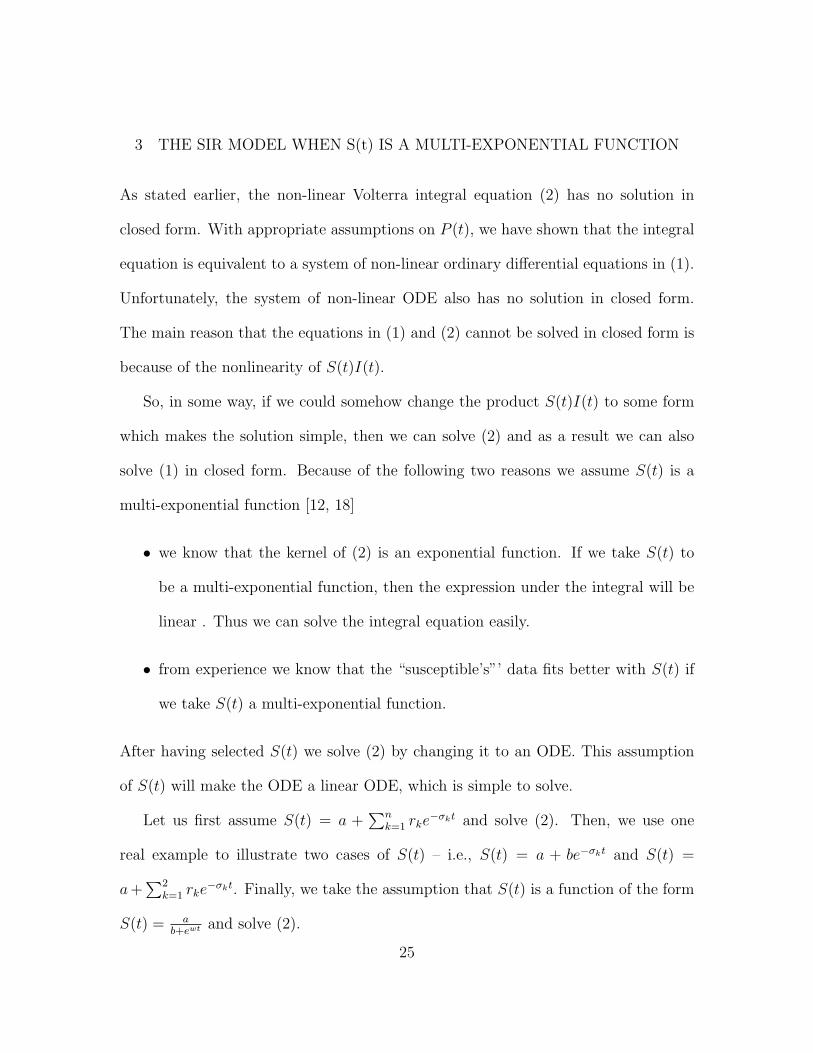
9 SIR Curves for Two Exponential S(t) . . . . . . . . . . . . . . . . . . 32
10 Best Fit Curve for Logistic Function . . . . . . . . . . . . . . . . . . 34
11 SIR Model Curves for Logistic Function . . . . . . . . . . . . . . . . 35
12 Data Fit Curve for “Recovery” Data . . . . . . . . . . . . . . . . . . 36
13 The Graph of β as a Function of Time . . . . . . . . . . . . . . . . . 37
7

1 INTRODUCTION
From pre-history to the present day, there have been many waves of epidemics
causing death and suffering of human beings. Most of these epidemics seemingly came
from nowhere, suddenly changed the normal demography of the affected population,
and ultimately disappeared before affecting the entirety of a population. This was a
puzzle for human beings for centuries, and there were many attempts to understand
these frequent epidemiological occurrences and to create a mechanism to control them
[2, 18].
• The first known result in mathematical epidemiology is due to Daniel Bernoulli.
In 1760 he formulated and solved a model for a smallpox epidemic [18].
• In 1906 William Hamer formulated a discrete time model for measle epidemics
[18].
• A significant contributor to compartmental-based epidemiological models was
the public physician R.A. Ross. In 1911 he proposed a differential equation
model for malaria as a host-reactor disease and won the second Nobel Prize in
Medicine [18].
• The classical SIR model as we know it today was first introduced by A.G.
Mckendrick and W.O. Kermack in 1927. These two public health physicians
extended the work of Ross and developed the concept of an epidemic threshold
[18].
8

Most epidemiological models start from the same basic premise that the popula-
tion can be subdivided into a set of distinct classes (compartments) depending upon
their experience with respect to the disease [18]. One line of investigation is to di-
vide the population under study into the three compartments of [18] “Susceptibles”,
“Infecteds” and “Recovereds.” The number of individuals in each compartment is
denoted by S(t), I(t) and R(t) respectively, where
• S(t) denotes the number of individuals who are “Susceptible” to the disease at
time t. That is, S(t) is the number of people in the population who are not
“infected” at the given time t but who are vulnerable to the disease.
• I(t) signifies the number of “infected” individuals who are infectious and able
to spread the disease to a susceptible.
• R(t) counts those in the population who are “recovered” from the disease and
are no longer “susceptible”. Thus they do not contribute to the spread of the
disease.
Such a model is called an SIR model.
A simple mathematical model of a natural phenomenon is meant to highlight
the existing qualitative behaviors of the phenomena, so that we omit most details.
As natural phenomena are influenced by a variety of internal and external factors,
taking all aspects of it and try to model as it is makes the model too complicated,
bulky, and is generally unwise, as it is common to end up with equation(s) which
are difficult or impossible to solve. So it is common to take certain assumptions in
modeling.
9

The SIR model is formulated under the following assumptions [2, 4, 18]:
• (I) The community size is constant and is sufficiently large over the duration of
the epidemic. We denote the number of population by N , where
N = S(t) + I(t) + R(t)
• (II) The susceptibles become infected at a percentage rate proportional to the
number of “infecteds”.
• (III) It is also assumed that the “infecteds” are uniformly distributed among
the “susceptibles”.
Remark
• Assumption (I) says that since the demography of a population does not change
significantly within a short period of time we ignore birth and immigration.
• We clearly know that the rate of leaving compartment at the beginning, middle
and end of the epidemic varies greatly. What assumption (II) says is that we
take the average (mean) number leaving compartments as a constant. This
assumption is reasonable if the population size is large, but it is not good if the
size of the population is small, since the random contact rate plays a significant
role for spreading the disease in small size population [1].
• In assumption (III) we ignored such factors as age, sex, social background,
seasons, geographical location, etcetera, which may affect the epidemic signifi-
cantly.
10

2 SIR EPIDEMIOLOGICAL MODEL
In this chapter we will study two equivalent ways of formulating the SIR model –
the ordinary differential equation form and the integral equation form. The integral
equation form of the SIR model is more general than the ordinary differential equation
form for the following two reasons [1]:
1. We can deduce the classical ordinary differential equation form of the SIR model
by assuming P (t) is exponentially distributed.
2. Different functional forms of the probability density function P (t) gives us al-
ternative types of the SIR model.
Even though the more realistic probability density function is the gamma distribution,
which presupposes the probability of leaving the class is a function of the time spent
within the class, the classical SIR model is based on the premise that the probability
of infection is exponentially distributed, which implies that the rate of transfer from
one compartment to the other is independent of the time spent within the class [1].
With this consideration, we recover the classical differential equation form of the SIR
model from the integral form. We will explore the relation between two variables
with the absence of the third one. What we do here is examine the relation between
“S” and “I” in the SI coordinate plane and the relation between “R” and “S” in the
RS coordinate plane. Such a study of the relation between two variables with the
absence of the third one is called Phase Plane Analysis for the model [18].
11

2.1 Two Formulations of the SIR Model
We will see two formulations of the SIR model. First we consider the differential
equation formulation and then we will see the integral equation formulation of the
SIR model.
2.1.1 The Classical Differential Equation Form of the SIR Model
In addition to the assumptions we made in Chapter 1, the SIR model also assumes
the following (see [2, 3, 4, 18] for additional discussion of these assumptions):
• f(I) = βI, where f(I) is an increasing function of “I” called the force of infection
and β is a constant called the infection rate. The infection rate tells us the rate
at which the “susceptibles” transfer into the “infecteds” group.
• Alternatively, f(I) = β (I/N), where I/N is the “infecteds” density in a popu-
lation of size N .
The relation between the compartments is assumed to be as follows:
• As the epidemic spreads those in “susceptibles” compartment transfer to “in-
fecteds” compartment at a rate of β , i.e. S ′ = −f(I)S.
• The “infecteds” compartment receives the outflow from the first , and it also
loses “infecteds” to the “recovereds” one at a rate of β, i.e. I ′ = f(I)S − αI
– The parameter α is called the removal rate of infection. It is the rate
by which the “infected” transfer into the “recovery”. The probability of
12

remaining “infectious” through time t is given by by P (t). 1/α =∫ t
0P (t)dt
gives us the average infectious period.
• The third one implies R′ = αI.
From the above premises we have
S ′ + I ′ + R′ = − β
NSI +
β
NSI − αI + αI
S ′ + I ′ + R′ = 0
which implies that S(t) + I(t) + R(t) is constant. In fact, from our assumptions
we know that at any given time “t”, S(t) + I(t) + R(t) = N. Then the classical
differential equation form of the SIR model can be summarized as
dI
dt=
β
NS(t)I(t)− αI(t)
dS
dt= − β
NS(t)I(t) (1)
dR
dt= αI(t)
2.1.2 The Integral Equation Form of the SIR Model
In this section we explore the Integral equation form of the SIR model (1). To be-
gin with, we derive the classic SIR model using an alternative approach. Specifically,
we begin with a modeling paradigm of the form
The number of “Infecteds”at time t
=Initial number of “Infecteds”
still “Infecteds” at t+
Those infected in [0, t]who remain infectious
If we take P (t) to be the probability that an “infected” at time t0 = 0 remains
13

infectious at time t, then the idea above is given mathematically by
I(t) = I(0)P (t) +
∫ t
0
βS(τ)I(τ)
NP (t− τ)dτ (2)
Equation (2) is a non-linear Volterra Integral equation [7].
2.1.3 Equivalence of the Differential and Integral Form of the SIR Model
We said that selecting different forms of P (t) gives us alternative types of the SIR
model. Let us revisit the result in (1) by showing that if we assume P (t) as expo-
nentially distributed that is, P (t) = e−αt, then we recover the classical exponentially
distributed SIR model. Substituting P (t) = e−αt into (2) we have
I(t) = I(0)e−αt +β
N
∫ t
0
S(τ)I(τ)e−α(t−τ)dτ (3)
Differentiating (3) with respect to t, we have
dI
dt=
β
NSI − α
[I(0)e−αt +
β
N
∫ t
0
S(τ)I(τ)e−α(t−τ)dτ
]which implies that
dI
dt=
β
NSI − αI.
The probability of being recovered at time t is given by Q(t) = 1−P (t). Differentiating
it we have
Q′(t) = αP (t)
which implies
dR
dt= αI
14

Finally, since S + I + R is constant, we know that S ′ + I ′ + R′ = 0, which in turn
implies that S ′ = −I ′ −R′. This results in
dS
dt= − β
NSI
which completes the equivalence of the two forms of the SIR model formulation.
2.2 Phase Plane Analysis
In this section, we will study the relationship between our variables, S and I in the SI
plane, and S and R in the RS plane. This is called phase plane analysis. Moreover,
we will also study one of the very important elements of epidemiology called the
reproductive rate of infection, commonly denoted by R0.
2.2.1 Phase Plane in SI Plane
The first two equations in (1) involves only S(t) and I(t). We examine them to study
what the solution looks like in the SI plane. Right at the beginning of the epidemic;
there is no “recovery”, i.e. R(0) = 0 , and let the number of “susceptibles” be given
by S0 and the number of “infecteds” be given by I0. Also let S∞ be the number of
people who will not be “infected” throughout the epidemic. Thus S0 + I0 = N .
Dividing the first equation by the second in (1) we have
dI
dS=
βSI − αI
−βSI
=α
βS− 1
dI
dS=
ρ
S− 1 (4)
15

where ρ = αβ
is the relative removal rate. Equation (4) is called the Phase portrait
for the epidemic, and solutions to the phase portrait are called Phase curves [18] and
can be obtained as follows
I =
∫ ( ρ
S− 1)
dS
= ρ ln(S)− S + C1
I = ρ ln(S)− S + N − ρ ln(S0) (5)
Figure 1: One Phase Curve in SI Plane
From Fig (1), we observe that
• the curve starts at (S0, I0), rises to a maximum, and proceeds to S∞. That
means the epidemic stops because of the lack of “infecteds”, not because every-
one will be sick.
16

• the epidemic obtains a maximum somewhere between S0 and S∞.
We can determine the maximum point as follows
dI
dS=
ρ
S− 1
Then, the critical value will be the solution of the equation
dI
dS= 0
which implies
ρ = S
To show that we have maximum value at ρ, we use the second derivative test. The
second derivative of I with respect to S is
d2I
dS2= − ρ
S2< 0
which is negative. Hence, a maximum occurs at S = ρ as shown in Fig (2).
The maximum value is
Imax = ρ ln
(ρ
S0
)− ρ + N (6)
2.2.2 Phase Plane Analysis in RS Plane
If we divide the second equation by the third one in (1), then we have
dS
dR= −βSI
αI= −ρS
17

Figure 2: Phase Curves in SI Plane
which leads to
S(R) = S0e−R
ρ (7)
Equation (7) implies that the RS phase curve exponentially decays, which means
that the number of “susceptibles” decays exponentially as a function of the number
of “recovereds” as shown in Fig (3) . To show mathematically our claim before that
in any epidemic there is always a part of the population which will not be “infected”
throughout the epidemic we use equation (7) as follows
S(R) = S0e−R
ρ ≤ S0e−N
ρ > 0
which give us
0 < S∞ ≤ N
18

We know that if t → ∞, then R → R∞ and I∞ = 0 implies R∞ = N − S∞. From
Figure 3: Phase Curves in RS Plane
this it follows that
S∞ = S0e−R∞
ρ
S∞ = S0e−N−S∞
ρ (8)
We can use this relation to calculate the value of S∞ and/or ρ if we know either of
the two.
2.2.3 The Basic Reproductive Rate of Infection R0
The basic reproductive rate, commonly denoted by R0, is also called the basic repro-
ductive number or the basic reproductive ratio [2, 18]. It is basically the expected
(average) number of secondary cases produced by a typical primary case in an entirely
19

“susceptible” population. The reproductive rate of infection R0 is mathematically ex-
pressed as
R0 =S0
ρ
which results in
R0 =βS0
α
The reproductive rate R0 is important for prediction of whether there will be epidemic
or not [2, 18].
Theorem 2.1 (Threshold theorem of Epidemiology)
If S0 ≤ αβ, then I(t) is monotonically decreasing. If S0 > α
β, then an epidemic occurs
in that the number of “infected” will increase to a maximum before dropping to 0 over
time.
The threshold theorem can be interpreted in the following way
• if S0 ≤ ρ which gives us R0 ≤ 1, then there is no epidemic.
• if S0 > ρ which implies R0 > 1, then there will be epidemic.
Thus, stopping an epidemic is usually related to reducing R0 to be below 1.
Consider equation (5) with I∞ = 0 and S(∞) = S∞. We have
I = ρ ln(S)− S + N − ρ ln(S0) (9)
I + S − ρ ln(S) = N − ρ ln(S0) (10)
If we take the limit as t goes to ∞, then we have
S∞ − ρ ln(S∞) = N − ρ ln(S0)
20

Which results in
ρ =N − S∞
ln(
S0
S∞
)Alternatively, suppose that the only type of data available is from hospital reports
of relevant admissions and releases. This type of data commonly reports the number
of recovered. We can also determine the average rate of “recovery” from the report.
So it is reasonable to find R0 using the hospital data.
Using S(R) = S0e−R
ρ , dRdt
= αI and I + S + R = N ;
dR
dt= α(N −R− S)
= α(N −R− S0e−R
ρ )
from which we obtain
R′ − αN + αR = −αS0e−R
ρ
e−Rρ =
αN − αR−R′
αS0
Taking the logarithm on both sides and simplifying, we have
ρ =−R
ln(
αN−αR−R′
αS0
) (11)
If we take the limit as t goes to infinity, then (10) will be equal to (9) since R′ ap-
proaches 0.
Let us consider the following example to illustrate the validity of our discussion.
We are going to use this example several times in the future discussion too [18].
21

EXAMPLE
A certain flu outbreak in English boarding school lasted for 14 days. The school has
a total of 763 students, of which 512 contracted the flu during that period. One boy
is known to have been the initial infected person thus giving us a given data set for
I(t).
We can calculate the value of S(t) numerically using the data. Thus, we have the
following values:
Table 1: The Number Of “Infected” And “Susceptible” Students
Days Infected Susceptible
0 1 7621 3 758.992 7 749.553 25 721.204 72 645.45 222 493.486 282 306.897 256 171.128 233 99.219 189 64.1810 123 46.5111 70 36.9912 25 31.5413 11 28.2714 4 26.23
Taking the following values for β, α and ρ as
β = 0.0021, α = 0.441, and ρ =α
β= 210
22

we obtain a reproductive rate of infection
R0 =S0
ρ= 3.63 > 1,
matching the fact that an epidemic did occur. Using (9),
ρ =763− 25
ln 76225
= 215.9745.
The phase curves in SI and RS are as follows:
1. The Phase curve in the SI plane is given by substituting, N = 763 and S0 = 762
in I = ρ ln(S)− S + N − ρ ln(S0).
Then, we have, I = 210 ln(S)−S + 763− 210 ln(762) whose graphs is shown in
Fig (4).
2. Phase curves in the RS plane are obtained by taking the second and the third
equation in (1), and assuming S(0) = S0 = 762 and R(0) = 0.
we have the following:
S(R) = S0e−R/ρ = 762e−R/210
Which gives us Figure (5).
23

Figure 4: Phase Curves in SI Plane
Figure 5: Phase Curves in RS Plane
24
3 THE SIR MODEL WHEN S(t) IS A MULTI-EXPONENTIAL FUNCTION
As stated earlier, the non-linear Volterra integral equation (2) has no solution in
closed form. With appropriate assumptions on P (t), we have shown that the integral
equation is equivalent to a system of non-linear ordinary differential equations in (1).
Unfortunately, the system of non-linear ODE also has no solution in closed form.
The main reason that the equations in (1) and (2) cannot be solved in closed form is
because of the nonlinearity of S(t)I(t).
So, in some way, if we could somehow change the product S(t)I(t) to some form
which makes the solution simple, then we can solve (2) and as a result we can also
solve (1) in closed form. Because of the following two reasons we assume S(t) is a
multi-exponential function [12, 18]
• we know that the kernel of (2) is an exponential function. If we take S(t) to
be a multi-exponential function, then the expression under the integral will be
linear . Thus we can solve the integral equation easily.
• from experience we know that the “susceptible’s”’ data fits better with S(t) if
we take S(t) a multi-exponential function.
After having selected S(t) we solve (2) by changing it to an ODE. This assumption
of S(t) will make the ODE a linear ODE, which is simple to solve.
Let us first assume S(t) = a +∑n
k=1 rke−σkt and solve (2). Then, we use one
real example to illustrate two cases of S(t) – i.e., S(t) = a + be−σkt and S(t) =
a +∑2
k=1 rke−σkt. Finally, we take the assumption that S(t) is a function of the form
S(t) = ab+ewt and solve (2).
25

3.1 Finite Multi-Exponential Form of S(t)
Let us consider S(t) to be a multi-exponential function of the form S(t) = a +∑nk=1 rke
−σkt. With this S(t), equation (2) becomes
I(t) = I(0)e−αt +β
N
∫ t
0
(a +
n∑k=1
rke−σkτ
)I(τ)e−(t−τ)dτ
Thus, the non-linear Volterra integral equation is changed to a linear one. To solve
it, we change it to an ODE of the form
dI
dt=
(β
N
(a +
n∑k=1
rke−σkt
)− α
)I(t)
dI
I=
(β
N
(a +
n∑k=1
rke−σkt
)− α
)dt
Integrating both sides leads to∫dI
I=
∫ (β
N
(a +
n∑k=1
rke−σkt
)− α
)dt + C2
ln |I(t)| = β
N
(at−
n∑k=1
rk
σk
e−σkt
)− αt + C2
To solve for I(t), we change both sides of the above expression to exponential function,
and then we have the following
I(t) = eβN
“at−
Pnk=1
rkσk
e−σkt”−αt+C2
To determine the constant C2, we use the initial condition I(0) = I0.
26

I(0) = e−βN
“Pnk=1
rkσk
”+C2
Thus we have
eC2 = I0eβN
“Pnk=1
rkσk
”
Hence we have the following for I(t)
I(t) = I0eβN
“at−
Pnk=1
rkσk
e−σkt”−αt+ β
N
“Pnk=1
rkσk
”
Our next step is to find the function R(t). We know that
dR(t)
dt= αI(t).
But I(t) = N −R(t)− S(t), so that
R′(t) = α (N −R(t)− S(t))
R′(t) + αR(t) = α (N − S(t))
Thus, it is a non-homogeneous linear ODE which can be solved first by determining
an integrating factor µ(t) as
µ(t) = eR
αdt = eαt
Using µ(t) = eαt, R′(t) + αR(t) = α (N − S(t)) becomes
(eαtR(t)
)′= αeαt
(N −
(a +
n∑k=1
rke−σkt
))
Integrating both sides of the above equation, we have
eαtR(t) = Neαt − aeαt − αn∑
k=1
rk
α− σk
e(α−σk)t + C3
27

Dividing both sides by eαt we have
R(t) = N − a− αn∑
k=1
rk
α− σk
e−σkt + C3e−αt
Now it remains to find C3. Using initial condition R(0) = R0, we have
R(0) = N − a− α
n∑k=1
rk
α− σk
+ C3
which implies that
C3 = R0 −N + a + αn∑
k=1
rk
α− σk
.
This completes our solution.
Let us revisit our example taking S(t) with one exponential function and sum of
two exponential functions.
3.1.1 Susceptibles as a Single Exponential
Let us assume S(t) as a function of the form S(t) = a+be−σt. Using the Fit command
in Maple software we fit the data with a curve of S(t) as shown in Fig (6). That gives
us the values of a, b, and σ. These values, as discussed and formulated in section
3.1, are used to determine the functions S(t) , I(t) and R(t). To have a better curve
which best fits our data, we divided the data into two and fit each of them with S(t)
type functions. That gives us two functions for each of S(t) , I(t) and R(t). These
functions approximate the number of “Susceptibles”, “Infecteds” and “Recovereds.”
respectively.
By what we formulated in Section 3.1, we have the following functions which give
28

Figure 6: Data Fit Curve for “Susceptible” for One Exponential
us Fig (7)
S1(t) = 762− 2.948e0.904t
S2(t) = 25 + 8820.803e−0.584t
I1(t) = e0.973t+0.007e0.904t+0.005
I2(t) = e−0.389t−31.704e−0.584t+8.807
R1(t) = 1 + 0.967e0.904t − 1.967e−0.441t
R2(t) = 763 + 27152.695e−0.584t − 18864.797e−0.441t
In addition, the Fit command and other statistics routines in Maple provide
measures of variance that can be used to validate the fits. Because the curves are
piecewise-defined, we did not measure confidence intervals for these fits. However,
correlations between the actual data and the predicted curves are each in excess of
29

0.98, and chi-square goodness of fit tests similarly confirm our results.
Figure 7: SIR Curves for One Exponential S(t)
3.1.2 Susceptibles as a sum of two Exponentials
Let us assume that S(t) is a function of the form
S(t) = a +2∑
k=1
rke−σkt.
Using the Fit command in Maple software we fit the “Susceptibles” data with curves
of S(t). The fit gives us the corresponding values of a, r1, r2, σ1, σ2. Using the
discussion and formulation of section 3.1 we can determine functions S(t), I(t) and
R(t) . To have a better curve which best fits our data we divided the data into two
and fit each of them with two different S(t). This gives us two functions for each of
S(t) , I(t) and R(t) which approximates the number of “susceptibles”, “infecteds”
and “recovereds”, respectively. As a result we have Fig (8).
The following functions are the result of what we have discussed in Section 3.1
30

Figure 8: Data Fit Curve for the “Susceptible” for Two Exponential
which results in Fig (9).
S1 = 762.5− 0.596e1.323t + 2.230× 10⁻⁷e8.701t
S2 = 15− 1000.752e−1×10⁵t + 3931.869e−0.446t
I1 = e0.914t+0.005e1.323t+1.455×10⁻²⁰e8.701t−0.454
I2 = e−0.409t+0.0002e−1×10⁵t−18.545e−0.446t+9.352
R1 = 674.679− 0.0001e−8×10⁵t + 2.429e−13.370t − 11844.678e−0.569t
R2 = 13.893 + 0.115e1.323t − 2.478× 10⁻¹⁹e7.048t − 19.612e−0.445t
Once again, the goodness of fit test shows that the fit is reasonable. Also, the
correlation was again in excess of 0.97.
31
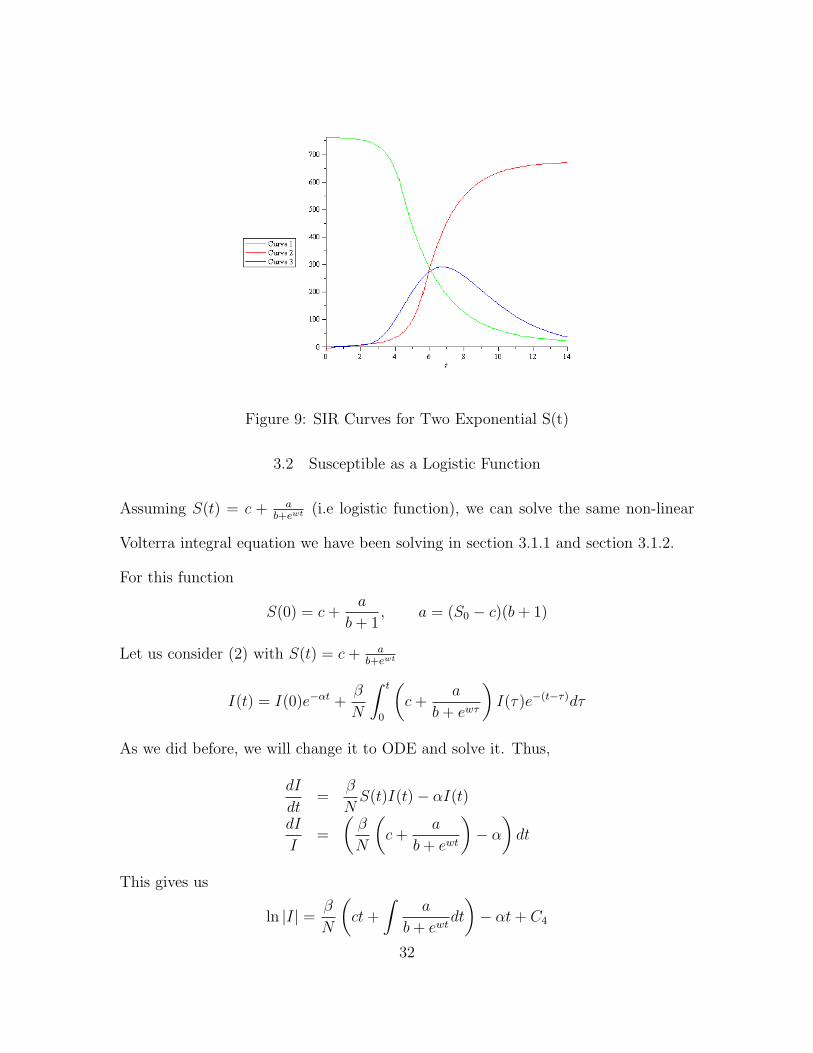
Figure 9: SIR Curves for Two Exponential S(t)
3.2 Susceptible as a Logistic Function
Assuming S(t) = c + ab+ewt (i.e logistic function), we can solve the same non-linear
Volterra integral equation we have been solving in section 3.1.1 and section 3.1.2.
For this function
S(0) = c +a
b + 1, a = (S0 − c)(b + 1)
Let us consider (2) with S(t) = c + ab+ewt
I(t) = I(0)e−αt +β
N
∫ t
0
(c +
a
b + ewτ
)I(τ)e−(t−τ)dτ
As we did before, we will change it to ODE and solve it. Thus,
dI
dt=
β
NS(t)I(t)− αI(t)
dI
I=
(β
N
(c +
a
b + ewt
)− α
)dt
This gives us
ln |I| = β
N
(ct +
∫a
b + ewtdt
)− αt + C4
32

If we late say u = b + ewt, then duw(u−b)
= dt and we have the following integral:
ln |I| = β
N
(ct +
a
w
∫du
u(u− b)
)− αt + C4
With this replacement, we have
1
u(u− b)=
−1b
u+
1b
u− b
from which we get
ln |I| = β
N
(ct +
a
w
(−1
b
∫du
u+
1
b
∫du
u− b
))− αt + C4
From this follows
ln |I| = β
N
(ct +
a
bw(ln |u− b| − ln |u|)
)− αt + C4
Changing the above to exponential function and replacing the value of u back produces
I(t) = eβN
“ct+ a
bwln
“ewt
b+ewt
””−αt+C4
To determine the constant C4 we use the initial condition I(0) = I0
eC4 = I0e− β
Na
bwln( 1
b+1)
Since we know I(t) and S(t) we can determine R(t) by
R(t) = N − I(t)− S(t)
which completes our solution.
Now we will consider the same example we have seen in section 3.1.1 and section
3.1.2. With c = S∞ = 25, and using command Fit in Maple we will have a function
33

Figure 10: Best Fit Curve for Logistic Function
which best approximates our data with functions of our form as shown in Fig (10).
Then, we have the following functions which gives us Fig (11):
S(t) = 25 +1.601× 10⁵
214.304 + e0.967t
I(t) = e−0.389t ln
“1.19e0.967t
214.217+e0.967t
”+0.005e0.967t
R(t) = 745.122− 1.601× 10⁵
214.304 + e0.967t− e
−0.389t ln“
1.19e0.967t
214.217+e0.967t
”+0.005e0.967t
Maple again not only reported the fit, but it also reported various measurements
of the goodness of the fit. The correlation is more than 0.98 and the chi-square
goodness of fit test confirmed our results. Also, we were able to obtain confidence
intervals for each of the parameters in the curve fits. Specifically, in S(t), we found
that the 95% confidence interval for w is [0.954, 0.989]. The 95% confidence interval
for a and b are nearly the same as the parameter values themselves. This shows that
34

Figure 11: SIR Model Curves for Logistic Function
the logistic function form for S(t) gives good results for the SIR model.
3.2.1 The Basic Reproductive Rate of Infection R0
The data we usually have for research purposes are data we get from hospitals re-
ports. This type of data commonly reports the number of “recovered”. We can also
determine the average rate of recovery from the report. Using the following equations
from our previous discussion;
dS
dt= −βSI
S + I + R = N
R′ = αI
35

Substituting I = R′
αin S = N − I −R, we have
β =R′′(t)
α+ R′(t)
N − R′(t)α−R(t)
We can use our example to show how we can apply the above equation. Fitting the
data with a function of the form
R(t) =a
b + ce−σt− d.
we have the fit curve Fig (12)
Figure 12: Data Fit Curve for “Recovery” Data
From Fig (12) we have a = 99175.54 , b = 138.99 , c = 26540.56, σ = −0.709 and
d = −3.717. Thus,
R(t) =99175.54
138.99 + 26540.56e−0.709t− 3.717
36

Figure 13: The Graph of β as a Function of Time
Using,
β =R′′(t)
α+ R′(t)
N − R′(t)α−R(t)
We have β = 0.001509. The graph of β is shown in Fig (13). This leads to the
approximation ρ = 220.5. Thus R0 = 3.45578.
37

4 CONCLUSION
The classical SIR epidemiological model is one of the earliest and most important
results of mathematical biology. It contains the most important features of epidemi-
ology namely “Susceptible”, “Infected” and “Recovered”. The basic SIR model has
its own limitation, but it is robust and can easily be extended. Depending on the
type of the disease under study, one can modify it to include some more aspects of
the disease. As a result we do have many variations of the model: SIS, SEIR, MSIR,
SIRS, SQIR.
Experiments with infectious disease in human populations is impossible and un-
ethical. Data are some times available from the natural occurrence of the epidemics.
Usually these data are incomplete and under reported. From experience, we know
that the data with all its weakness fits better with the results of this thesis’s functions
; S(t), I(t) and R(t). This gives us a way to closely study and interpret the data so
that we can make decisions to control a similar epidemic.
• As observed before, to find the appropriate multi-exponential S(t) = a +∑nk=1 rke
−σkt to fit our data better, we may need to partition the data to two
or more than two parts and fit each to a function and then we combine them.
• The other result discussed here is that of assuming S(t) = ab+ewt which is com-
monly called the logistic function. In this case, to find the function which best
fits the data, one should give initial values for variables a and b when using the
Fit command with Maple software.
38

• After selecting S(t), one can use all the results of this thesis to study the
important features of the disease. As a result, it helps us to design the analysis
of epidemiological surveys, suggest crucial data that should be collected, identify
trends, and forecast and estimate uncertainty.
While we are working with this thesis we have observed that the data collected from
an epidemic fits nicely with the function of a difference of two logistic functions for
the “infectious” data. In case somebody has “infected” population data and wants
to know whether there was epidemic or not, he/she can start from that and do what
has been done in this thesis. In reality, most data reported from sources indicates
the “recovered” population number. One can also start from “recovered” populations
data and study the SIR model.
39

BIBLIOGRAPHY
[1] Helen J.Wearing, Pejman Rohani and Mat J.Keeling, Appropriate Model For
The Management of Infectious Disease, PLoS Med 2, No.7, e174, 2005.
[2] Teri Johnson, Mathematical Modeling of Disease. Susceptible-Infected-Recovered
(SIR) model, Math 409 Senior Seminar, University of Minnesota , 2009.
[3] Vrushali A Boki, Lecture Note, Introduction to the Mathematics of Infectious
Disease, Oregon State University, Corvallis, Oregon, August 1, 2007
[4] David Smith and Lang Moore, The SIR model for spread of Disease,
www.math.duke.edu/education/ccp/materials/diffcalc/sir/index.html, Duke Uni-
versity, Last Accessed July 30, 2010.
[5] Modification of the SIR model, www.math.lsa.umich.edu/ tjacks/sirlecs.ppt.,
Last Accessed July 6, 2010.
[6] Abdul-Majid Wazwaz, A First Course in Integral Equation, World Scientific
Publishing, 15-20, 1997
[7] F. G. Tricomi, Integral Equation, Dover Publication Inc., 1-42, 1985
[8] Rainer Kress, Linear Integral Equation, Second Edition, Springer-Verlag Inc.,
1-13, 1999
[9] Ram P.Kanwal, Linear Integral Equations, Theory and Techniques, Second Edi-
tion, The Random house Birkhauser Mathematics Series, 25-36, 1997
40

[10] Ida Del Prete, Efficient Numerical Methods For Volterra Integral Equation of
Hammer Stein type, Universita Di Napoli Federico II, 1-16, 2006
[11] Herbert W.Hetthcote, Quantitative Analysis of Communicable Disease Model,
Mathematical Biosciences 28, 335-356 , 1976
[12] Christopher D. Green, Integral Equation Methods, Barnes and Noble Inc., 81-90,
1969
[13] M.Krasnov, A.Kieslev and G.Mkarenko, Problems and Exercises in Integral
Equations, Mir Publisher, 15-62, 1971
[14] Gustav Doestsch, Guide to the Application of the Laplace Transform and Z
Transform, Second Edition, Van Nostrand Reinhold Company, 118-121, 1971.
[15] Joel L.Schiff, The Laplace Transform Theory and Application, Springer-Verlag
Inc., 1-34, 1999.
[16] S.Patrak, A.Maiti, G.P. Samanata, Rich Dynamics of an SIR epidemic model,
Nonlinear Analysis, Modeling and Control 15, 71-81, 2010
[17] Michael Holile, Population Dynamics I, The SIR model, Department of Animal
Science and Health, Royal Veterinary and Agriculture University, 2002
[18] Fred Brauer and Carlos Castillo-Chavez, Mathematical Models in Population
Biology and Epidemiology, Springer-Verlag Inc., 273-332, 2001
41

APPENDICES
Appendix MAPLE COMMANDS
1. TO PRODUCE FIGURE 6
dataplot := ScatterPlot(A, B, symbol = diamond, symbolsize = 20, color = blue);
S0 := Fit(762+C[1]*exp(-aa[1]*t), A[1 .. 6], B[1 .. 6], t, initialvalues = [C[1] = -
1.52181363299841910, aa[1] = 1.0852]);
S1 := Fit(25+C[1]*exp(-aa[1]*t), A[6 .. 13], B[6 .. 13], t, initialvalues = [C[1] = 100,
aa[1] = 10−5]);
l0 := plot(S0, t = 0 .. 5, color = green);
l1 := plot(S1, t = 5 .. 14, color = green);
d1 := display(l0, l1);
display(dataplot,lo,l1)
2. TO PRODUCE FIGURE 7
a1 := 762; b1 := -2.94757082275819516; sigma1 := -.903717448872219053;
a2 := 25; b2 := 8820.8029307937304; sigma2 := .584262909390753205;
I1 := exp(beta*a1*t/(1.132)+beta*b1*exp(-sigma1*t)/sigma1-alpha*t+beta*b1/(1.35*sigma1));
I2 := exp(beta*(a2*t-b2*exp(-sigma2*t)/sigma2)-alpha*t+beta*b2/(3.6*sigma2));
P1 := plot(I1, t = 0 .. 3.81, color = blue);
P2 := plot(I2, t = 3.81 .. 14, color = blue);
42

R2 := N-alpha*b2*exp(-sigma2*t)/(alpha-sigma2)+(-N+alpha*b2/(3/2*(alpha-sigma2)))*exp(-
alpha*t);
R12 := plot(R2, t = 6.1 .. 14);
R11 := plot(R1, t = 0 .. 6.2);
d := ScatterPlot(A, R, symbol = diamond, symbolsize = 20, color = blue);
display(d1, d2, d3, linestyle = solid, color = [red, blue, green]);
3. TO PRODUCE FIGURE 8
S011 := Fit(762.5+C11*exp(-a11*t)+C21*exp(-a21*t), A[1 .. 6], B[1 .. 6], t,
initialvalues = [C11 = -1.52181363299841910, a11 = 10.0852, C21 = -2.1, a21 = -10]);
S11 := Fit(15+C12*exp(-a11*t)+C22*exp(-a21*t), A[5 .. 14], B[5 .. 14], t,
initialvalues = [C12 = -1000.75181363299841910, a11 = 100000.0732, C22 = 3000,
a21 = -.9]);
dtplot := ScatterPlot(A, B, symbol = diamond, symbolsize = 20, color = blue);
l01 := plot(S011, t = 0 .. 4.2, color = green); l11 := plot(S11, t = 4.2 .. 14,
color = green); se := display(l01, l11);
g := 15; r11 := -1000.75181363299998; r21 := 3931.86878378646998;
σ 11 := 1.00000073199999999*105; σ 12 := .445677297008923612;
f := 762.5; r1 := -.595872937335464426; σ 21 := -1.32299589086598157;
r2 := 2.23037891409369903*10−17; σ 22 := -8.70076794567668976;
I21:=exp(.901*β*(f*t-2*r1*exp(-σ21*t)/σ 12-3*r2*exp(-σ 22*t)/σ 22)
-1.2*α*t+β*(r1/σ 21+r2/σ 22))-.45399;
43

I22 := exp(1.001*β*(g*t-r11*exp(-σ 11*t)/σ 11-r21*exp(-σ 12*t)/σ12)
-α*t+5.87*β*(r11/σ21+1/σ12));
u1 := plot(I22, t = 2.5 .. 14, color = blue);
u2 := plot(I21, t = 0 .. 2.5, color = blue);
Ie := display(u1, u2);
display(dtplot, l01, l11);
4. TO PRODUCE FIGURE 9
R77 := 1.0022*N-6*g-29*α*r11*exp(-8*σ11*t)/(2*N*(α-σ11))-α*r21*exp(-30*σ
12*t)/(200*N*(α-σ12))+(-(19/2)*N+(35/2)*g+(6*9)*α
r11/(2*N*(α-σ11))+10*α
r21/(N*(α-σ12)))*exp(-1.29*α*t);
R21 := 1.011*N-f-α*r1*exp(-.999987*σ21*t)/(1.3*(α-σ21))-α*
r2*exp(-.81*σ22*t)/(22.5*(α-σ21))+(-1.025*N+f+α*r1/(4*(α-σ21))
+α*r2/(α-σ22))*exp(-1.01*α*t)+5;
R9 := plot(R21, t = 0 .. 5.56, color = red);
R99 := plot(R77, t = 5.6 .. 14, color = red);
Ree := display(R9, R99);
display(Ie, Ree, se, linestyle = solid);
5. TO PRODUCE FIGURE 10
S4 := Fit(25+a/(b+exp(w*t)), A, B, t, initialvalues = [a = 200000, b = 1, w = .3]);
ScatterPlot(A, B, plot(S4, t = 0 .. 14));
44

6. TO PRODUCE FIGURE 11
a1 := 1.60081881732383365∗105; b1 := 214.217265807576496; w1 := 0.967296187971025124;
I4 := exp(β*(25*t+a1*ln(1.19*exp(w1*t)/(b1+exp(w1*t)))/b1)-alpha*t-β*a1*ln(1/(b1+1))/b1);
ScatterPlot(A, Dat, plot(I4, t = 0 .. 14));
R4 := N-S4-I4+7.122246889;
plot([S4, I4, R4], t = 0 .. 14, linestyle = [solid, solid, solid], color = [red, blue, green]);
45

VITA
TESHOME MOGESSIE BALKEW
Education: B.S. Mathematics, Addis Ababa University in Ethiopia,
Addis Ababa, Ethiopia, 1989
M.S. Mathematics, Addis Ababa University
Addis Ababa, Ethiopia, 1998
M.S. Mathematical Sciences, East Tennessee State University
Johnson City, Tennessee, 2010
Professional Experience: High School Teacher, Wachemo Cop.Sec.School In Ethiopia
Hossana, Ethiopia, 1989–1995
Lecturer, Alemaya University
Alemaya, Ethiopia, 1998-2002
Lecturer, Addis Ababa University
Addis Ababa, Ethiopia, 2002-2008
Graduate Assistant, East Tennessee State University
Johnson City, Tennessee, 2008-2010
46